


Abstract
Tree ensembles predict product quality accurately from process-condition data but are opaque, and rule extraction addresses this by compressing an ensemble into a small set of decision rules. A ruleset, however, is a technical representation, and the operators, production managers, and data scientists who act on a quality prediction each require something different from the same ruleset. Small language models deployed on local hardware can express a rule in the terms each audience requires, but they carry little process-specific knowledge and must therefore be grounded in context supplied at inference time. Systems of this kind often supply all available context by default, but the value of this has not been tested. This study presents RuleSLM, which grounds a compact language model in a ruleset extracted from an XGBoost model trained to detect sink mark defects in injection moulding, and decomposes the supplied context into rule evidence, knowledge, and interaction guidance. Crossing the latter two in a factorial design over four small language models and 58 role- and intent-annotated questions shows that interaction guidance increases the evaluator’s role-appropriateness score by 0.323 points on a five-point rubric, that knowledge context changes no dimension measurably, and that the two components interact in opposite directions on different models. Supplying the full context increases the input length by 275% and energy per response by 50% for a benefit confined to one of three quality dimensions. Repeated evaluation further shows that the rubric-based evaluator reproduces fewer than half of the individual scores while producing configuration-by-dimension means that are stable to within 0.12 points. Context for rule-grounded explanation should therefore be selected for the property it serves and validated on the model that will be deployed.
1. Introduction
Quality prediction has become a fundamental pillar of modern manufacturing. As product complexity increases and tolerance windows shrink, manufacturers require accurate and proactive quality assurance strategies. Sensor-rich equipment and Industrial Internet of Things platforms now supply large volumes of condition-monitoring and process data, which can be used to anticipate defects before they occur and thereby reduce rework, shorten cycle times, and improve product consistency. The feasibility of applying machine learning to quality-related tasks has been demonstrated in injection moulding, machining, die casting, and predictive maintenance [1,2,3,4]. The models that achieve the highest predictive accuracy in these settings, particularly tree ensembles and deep neural networks, are also the least transparent, which limits their adoption in environments where automated decisions must be justified to auditors, engineers, and machine operators [5,6,7].
Explainable artificial intelligence (XAI) addresses this limitation through methods that expose the decision behaviour of an opaque model. Among them, rule extraction produces a surrogate model in the form of a small, ordered set of if–then rules that reproduces the predictions of the original ensemble closely enough to stand in for it during inspection. RuleCOSI+ [8] compresses a tree ensemble of several hundred rules into a handful of conditions on named process variables, each annotated with the fraction of training instances it covers and the fraction of those instances it classifies correctly. The result is auditable and compact.
A ruleset, however, is not yet an explanation. It is a technical representation written in the vocabulary of the model, and the people who act on a quality prediction do not share that vocabulary or that purpose. A machine operator needs to know which process conditions are associated with the prediction and how they relate to the settings under their control. A production manager needs the same prediction framed as evidence for a decision, with an indication of how broadly it applies. A data scientist needs the split points, the class distributions, and the limits of what the training evidence supports. A single rendering of a rule cannot serve all three. Rule extraction therefore does not close the explanation gap. It relocates it from the ensemble to the ruleset.
Language models offer a way to close it, by expressing the same rule in the terms each audience requires [9,10]. Frontier-scale models are nevertheless impractical in many production environments, where data confidentiality, network isolation, per-query cost, and latency favour on-premises inference. Compact open-weight small language models (SLMs) in the 1B–3B parameter range [11,12,13,14] run on a single workstation GPU and are the realistic deployment target. Because a model of this size carries little process-specific knowledge in its parameters, everything it asserts about a particular machine, dataset, or ruleset must be supplied to it at inference time as explicit context.
This raises a question that has not been examined. Systems of this kind supply all available context by default, on the assumption that more grounding produces better explanations. Context is not free. Every additional context item lengthens the prompt, and prompt length propagates directly into latency, memory occupancy, and energy consumption on the constrained hardware that motivated the choice of a compact model in the first place. More context is also not necessarily beneficial, since information that serves one property of an explanation may do nothing for another, or may interfere with it. No controlled study has established which context contributes to which property.
Accordingly, this study decomposes the context supplied to the generator into three functional groups: rule evidence (R), the extracted ruleset that the explanation is about; knowledge (K), the process, dataset, and model descriptions that give the rule its meaning; and interaction guidance (G), the stakeholder profile and question intent that determine how the answer should be expressed. Holding R present in every configuration and crossing K and G yields a factorial design that isolates the contribution of each. Three research questions follow:
- RQ1. Does knowledge context improve the factual grounding and completeness of generated explanations?
- RQ2. Does interaction guidance improve the appropriateness of explanations for the target role?
- RQ3. Do knowledge context and interaction guidance interact, and is any such interaction consistent across model families and scales?
To answer these questions we conducted a factorial experiment on an industrial injection moulding dataset. A tree ensemble for quality prediction was trained with XGBoost [15] and a compact ruleset was extracted from it using RuleCOSI+ [8], forming the rule evidence group R. The remaining context was supplied as structured cards grouped into knowledge (K) and interaction guidance (G). A benchmark of 58 role- and intent-annotated questions, each paired with a curated reference answer, was presented to four instruction-tuned small language models from three families, namely, Llama-3.2 (1B and 3B), Qwen2.5 (1.5B), and Gemma-2 (2B), under four context configurations: R alone, R + K, R + G, and R + K + G. The resulting 928 explanations were scored on three rubric dimensions by Prometheus 2 (7B) [16] operated deterministically, with the curated reference answers scored under the same rubrics to establish the attainable range of the instrument. Interaction guidance increased the evaluator’s role-appropriateness score, with no statistically detectable average change in the other dimensions, whereas knowledge context changed no dimension measurably while costing half again as many input tokens. The two groups interacted in opposite directions on different models, so no single configuration was best for all four.
The contributions of this study are threefold:
- 1.
- A functional decomposition of generation context for rule-grounded explanation, together with a factorial design that measures the contribution of each component to explanation quality and to deployment cost.
- 2.
- A benchmark of 58 role- and intent-annotated questions over an industrial injection moulding ruleset, with curated reference answers, and a frozen three-dimension evaluation protocol whose attainable range is calibrated against those references.
- 3.
- An empirical characterisation of context effects across four small language models from three families, covering explanation quality, evaluator reliability, and the inference cost of each configuration.
The remainder of this paper is organised as follows. Section 2 reviews explainable AI in manufacturing, rule extraction, small language models for industrial deployment, contextual grounding, and the evaluation of generated explanations. Section 3 presents the RuleSLM framework and the decomposition of its context layer. Section 4 describes the case study, the question benchmark, the experimental conditions, and the evaluation protocol. Section 5 reports the results. Section 6 discusses their implications and the limitations of the study, and Section 7 concludes.
2. Background and Related Work
This section reviews the research streams on which RuleSLM builds: explainable AI for manufacturing quality prediction, rule extraction and surrogate modelling, small language models as an explanation interface, contextual grounding of language models, and the evaluation of generated explanations. Concepts from XAI and language modelling that recur throughout the paper are introduced where they first appear.
2.1. Explainable AI in Manufacturing Quality Prediction
Quality prediction models relate high-dimensional process measurements, such as temperature, pressure, speed, and cycle timing, to inspection outcomes. Higher-capacity models, particularly tree ensembles and deep networks, capture the dependencies among these variables more effectively than statistical process control or single decision trees, and have been applied to defect detection and dimensional stability across machining and injection moulding [4,7,17]. Deployed systems demonstrate measurable operational benefit; for example, a real-time prediction pipeline applied across three injection moulding machines increased overall equipment effectiveness and reduced non-conforming parts, using human-in-the-loop labelling to address the difficulty of collecting balanced defect data on the shop floor [18]. Label scarcity in continuous-flow processes has been addressed by combining semi-supervised learning with recurrent time-series prediction [19], and few-shot approaches have been proposed for injection moulding where defect examples are scarce [20].
Predictive gains come at the cost of transparency. Post hoc XAI methods, meaning methods applied to an already trained model without altering it, address this through feature importance rankings, partial dependence plots, individual conditional expectation curves, and SHAP values [5,21]. Surveys of XAI in manufacturing and industrial cyber–physical systems report that deployed techniques remain predominantly model-centric, with little attention to tailoring explanation content or delivery to distinct end users [22]. A patent-based review of industrial deployment reinforces this from a practitioner perspective, where SHAP and LIME are adopted to support operator trust, they are often not suited to real-time environments, and a mismatch between explanation modality and operator need can reduce trust instead of building it [23]. It has been argued that human-centred explanation requires actionable and contextually situated reasoning, not only interpretability of the model [24].
The stakeholders who use a manufacturing quality prediction have distinct informational needs. Operators require concise operational guidance framed in plant vocabulary; managers require performance and risk framing suitable for decisions and reporting; data scientists require model behaviour, rule statistics, and generalisation limits. Existing rule-based approaches in injection moulding provide interpretable insight into defect formation [1] but produce one static rendering irrespective of who is reading it. Recent surveys have identified role-aware, contextually grounded explanation as a persistent gap [7].
2.2. Rule Extraction and Surrogate Models
A surrogate model is a simple model trained to reproduce the input–output behaviour of a complex one, so that the surrogate can be inspected in place of the original. The quality of this substitution is measured by fidelity, the proportion of instances on which the surrogate and the original model produce the same prediction. Fidelity is distinct from accuracy because a surrogate can agree closely with a model that is itself wrong.
Rule extraction produces surrogates in the form of if–then rules. RuleFit [25] transforms tree ensembles into rules fitted with a sparse regressor, but yields rulesets too large to inspect, while inTrees [26] prunes and summarises extracted rules at some cost in predictive performance. RuleCOSI+ [8] combines and simplifies the split values discovered by the ensemble into a single ordered decision list, retaining predictive behaviour comparable to the original ensemble with a small number of rules. Optimisation-based formulations pursue the same objective by other means. FIRE poses rule-ensemble extraction as a sparsity-constrained problem [27], and integer-programming formulations jointly optimise the number of rules and their interaction depth, making the trade-off between fidelity and interpretability explicit [28].
Each extracted rule additionally carries statistics describing the training evidence behind it, namely, its coverage, confidence, and support, which are defined in Section 3.2. These quantities are what an explanation must convey when a stakeholder asks how far a prediction can be relied upon.
Rule-based surrogates suit industrial settings because their decision logic is explicit and auditable. In RuleSLM, the extracted rules serve as the evidence that generated explanations must remain consistent with.
2.3. Small Language Models as an Explanation Interface
Language models generate text conditioned on an input sequence. What they can assert comes from two sources: parametric knowledge, acquired during pretraining and stored in the model weights; and information supplied in the input at inference time. This distinction is central to the present work. A specific injection moulding machine, its feature set, and a ruleset extracted from a particular ensemble are absent from any pretraining corpus, so a model can only describe them from what it is given.
Frontier-scale models have been applied to manufacturing decision support, with frameworks such as LLM-MANUF integrating domain data with generative reasoning [9]. Their computational demands and reliance on cloud infrastructure conflict with the operational constraints of many production environments. This has motivated work on small language models (SLMs), typically open-weight models below roughly 5B parameters that run on commodity or edge hardware [11]. Recent families, including Llama-3.2 [12], Qwen2.5 [13], and Gemma-2 [14], combine instruction-following ability with modest memory footprints, and quantisation, which stores model weights at reduced numerical precision, brings models of this size within the memory budget of a single workstation GPU. A benchmark of more than sixty publicly available SLMs reports that current models in this range match or exceed the general-task performance of earlier 7B models [29].
Evidence on how these families behave on grounded industrial tasks remains scarce. Existing SLM benchmarks emphasise general capabilities such as commonsense reasoning, mathematics, and coding [11,29], leaving open the issue of whether conclusions transfer to tasks in which the output must remain consistent with an external symbolic representation, like a ruleset. Effects that are well documented at the frontier scale may also manifest differently at the small scale, where limited capacity can make a model either more dependent on supplied context or more easily destabilised by it.
2.4. Grounding Generation in Supplied Context
Contextual grounding supplies structured external information in the prompt so that generated text reflects that information instead of the model’s parametric priors. Retrieval-augmented generation [30] is the most widely studied instance, in which passages retrieved from a corpus are prepended to the query. The setting considered here differs because the relevant contextual materials are known in advance and prepared once. These include a ruleset, a dataset description, a process description, and a stakeholder profile. No retrieval step is therefore required. Instead, the main design question is which of these materials should be supplied to the model.
That question is normally answered by supplying all of them. The cost of this is measurable. Prompt length determines the time to first token, the memory occupied by the attention cache, and the energy consumed per response, all of which matter on the hardware that on-premises deployment implies. The benefit is less clear. Structured context is heterogeneous in function: a process description supports factual claims, whereas a stakeholder profile governs vocabulary and emphasis. Whether these functions are separable, and whether supplying one improves properties governed by the other, has not been tested under controlled conditions. Existing work supplies context and evaluates the resulting output; the present study varies the context and measures the consequence.
2.5. Evaluating Generated Explanations
Doshi-Velez and Kim [31] distinguish three levels of interpretability evaluation: application-grounded, with domain experts performing real tasks; human-grounded, with simplified tasks and lay participants; and functionally grounded, which uses quantitative proxies without human subjects. The present study is functionally grounded, since its objective is a controlled and reproducible comparison of configurations.
Automatic evaluation of generated text is nevertheless difficult for explanations. Reference-based measures compare a candidate against a curated answer: lexical overlap metrics such as BLEU [32] and ROUGE [33] count shared n-grams, while embedding-based measures such as BERTScore [34] and SBERT cosine similarity [35] compare distributed representations. An explanation can be entirely correct while sharing little surface form with its reference, particularly when the same rule is rendered for different audiences, so these measures bound explanation quality only loosely. Recommendations on automatic evaluation accordingly advise combining complementary measures and interpreting each within its stated scope [36].
Rubric-based automatic evaluation addresses this by prompting a language model to score a response against explicit criteria, a protocol commonly termed LLM-as-a-judge [37]. The evaluator is itself a model, which introduces two requirements that this study treats as part of the protocol. The scoring instrument must be fixed before the outputs it will score are produced, and the attainable range of its scale must be established, since a rubric score has no absolute meaning without knowing what a strong answer receives under the same instrument. Both are addressed in Section 4.7.
2.6. Research Gaps
Three gaps follow from the lines reviewed above. First, explanation in manufacturing remains single-audience: rule surrogates and post hoc XAI tools produce one static output without adapting the content and depth to the operator, manager, or data scientist consuming it [1,2,7]. Second, small language models are established as viable on general benchmarks, but controlled comparisons on grounded industrial generation tasks that must remain consistent with an external symbolic representation are scarce [11,29]. Third, and most directly addressed here, systems that ground generation in structured context supply that context as an undifferentiated bundle, without evidence on which components contribute to which properties of the resulting explanation, or at what cost. Broader surveys of language model adoption across engineering disciplines identify the same structural shortcomings, namely, the absence of domain-specific benchmarks and validation protocols suitable for precision-critical settings [38], suggesting that these are properties of current deployment practice and not artefacts of one application area.
3. The RuleSLM Framework
RuleSLM produces role-adaptive natural language explanations of manufacturing quality predictions by grounding a compact language model in an extracted ruleset and a set of structured context inputs. This section presents the framework and its context-layer decomposition, which is evaluated experimentally in this study. The framework is agnostic to the generative model, which means that any sufficiently capable instruction-tuned language model can occupy the explanation layer. The specific models compared in this study are described in Section 4.
3.1. Overview and Notation
Figure 1 situates RuleSLM within a conventional quality prediction pipeline followed by an explainability layer. The pipeline collects sensor data during production, aggregates it into a per-cycle feature representation, trains a predictive model that outputs a quality class, and extracts a simplified ruleset as an interpretable surrogate. Context assembly groups the surrogate ruleset and the remaining context inputs into the three functional sets R, K, and G. Generation conditions a small language model on the selected context together with a stakeholder role and a question, and the resulting explanation is scored on three rubrics by an evaluator model. Each phase is described in the following subsections.
Figure 1.
The RuleSLM framework. The extracted ruleset supplies rule evidence (R) in every configuration; knowledge (K) and interaction guidance (G) are supplied conditionally. A small language model generates an explanation for the specified role and question, and an LLM-based evaluator scores it on three rubric dimensions. The rules shown are illustrative.
The notation used throughout the paper is introduced here and reused in the experimental sections. Let denote the feature space of per-cycle process measurements and the set of quality classes. Let denote the language model that occupies the explanation generation layer, u a user or stakeholder profile, q a question, and e the generated explanation.
3.2. Prediction and Rule Extraction Layer
The predictive model is a tree ensemble trained on features derived from the process signals recorded during each production cycle. A rule extraction algorithm is then applied to it to produce a compact ruleset that reproduces its decision behaviour, as stated in Definition 1.
Definition 1
(Rule Extraction as Functional Approximation). Let be a trained black-box predictive model and let be a ruleset extracted from f. Each rule takes the form
where is a conjunction of conditions on the input features and is the consequent class label. The ruleset induces an interpretable rule-based model constructed such that
The quality of this approximation is quantified by the fidelity
the proportion of held-out instances on which the surrogate and the original model agree.
Fidelity is reported alongside predictive accuracy in Section 5.1, since the explanations describe the behaviour of f and not the quality of the product directly.
Beyond its consequent, each rule carries statistics describing the training evidence behind it. Let be the training set with records. The coverage of a rule is the fraction of records falling in the feature space region defined by its antecedent, that is, , where is the number of records satisfying .
The confidence of is the fraction of the records it covers that also agree with its consequent, that is, , where is the number of records satisfying both. The support of is the fraction of records satisfying both, , so that and support and coverage coincide when a rule is perfectly confident. In an ordered decision list these quantities are computed on the records reaching , that is, those not already covered by a preceding rule.
In RuleSLM the ruleset is extracted with RuleCOSI+ [8], which represents the result as an ordered decision list. Rules are evaluated in sequence and the consequent of the first rule whose antecedent is satisfied determines the prediction; a default rule applies when no preceding rule fires. Each rule is encoded with a rule identifier, its antecedent conditions, its consequent class, and the training statistics defined in Section 2.2: coverage, confidence, support, and the class distribution of the covered instances. These statistics provide reliable evidence that the explanation generation model must use and properly convey whenever a stakeholder asks how reliable a prediction is.
3.3. Context Assembly Layer: Functional Decomposition
The extracted ruleset states which conditions lead to which prediction, but it does not state what the features mean, how the process behaves, how the ruleset should be read, who is asking, or what kind of answer the question calls for. RuleSLM supplies this information as six structured JSON contextual cards, each authored once per deployment. The cards are grouped by function into three sets, summarised in Table 1. The complete contextual cards and generation prompt are provided in Supplementary File S1.
Table 1.
Functional decomposition of the RuleSLM context layer. The rule evidence group is present in every configuration; the knowledge and interaction guidance groups are supplied conditionally.
3.3.1. Rule Evidence (R)
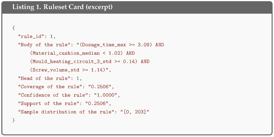
The Ruleset card (Listing 1) encodes in the representation described in Section 3.2. It is supplied in every experimental configuration, since an explanation of a prediction with no access to the rule that produced it would have no evidential basis at all.
3.3.2. Knowledge (K)
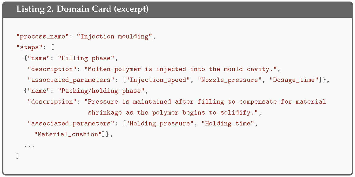
The Dataset card describes the data from which the predictor was built: the number of predictive features, the training and testing instance counts, the split strategy, the meaning of the statistical suffixes attached to feature names, and the semantics of the output classes. The Domain card (Listing 2) encodes process knowledge independent of any dataset or model, namely, the description of injection moulding, its operational phases, the process parameters associated with each phase, and the defect types that can arise. The Model card describes the structure of the rule-based surrogate itself: the parts of a classification rule, the meaning of each rule statistic, and the procedure for applying an ordered decision list to a new instance. Together these three cards allow the generator to state what a feature such as Material_cushion_median refers to, which phase of the process it belongs to, and what a confidence of 1.0000 signifies.
3.3.3. Interaction Guidance (G)
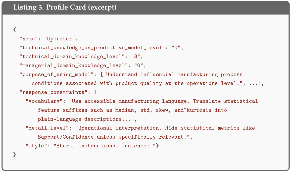
The Profile card (Listing 3) defines the three stakeholder roles targeted by RuleSLM. Each role is characterised along three independent expertise dimensions: technical knowledge of the predictive model, technical domain knowledge, and managerial domain knowledge; rated on a four-level novice-to-expert scale: level 0 for novice, level 1 for advanced beginner, level 2 for competent, and level 3 for expert. Each profile also states the purpose for which the role consults the model and the constraints on vocabulary, detail level, and style that follow from it. The Intent card defines the question types the assistant is expected to handle and, for each, the shape of an appropriate answer per role. Section 3.4 develops this taxonomy.
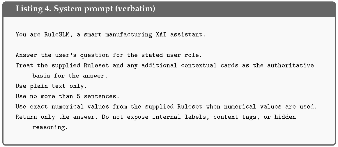
Output-format requirements that apply to every answer, such as the maximum response length and the prohibition on markup, are specified in the system prompt (Section 3.5) and are therefore identical in all configurations. The three groups differ in content, not in the form of the answer they request.
Definition 2
(Context-Conditioned Explanation Generation). Let , , and denote the card sets of the rule evidence, knowledge, and interaction guidance groups. A context configuration is a subset , and the context supplied under γ is
Given a user or stakeholder profile u and a question q, the explanation is generated as
Because for every γ, all configurations share the same evidential basis and differ only in the interpretive and communicative context accompanying it.
3.4. Stakeholder Profiles, Question Intents, and Explanation Goals
The interaction guidance group encodes two distinct things: who is asking, and what they are asking for. Neither alone determines an appropriate answer. A question about the confidence of a rule calls for different content when raised by an operator seeking reassurance than when raised by a data scientist assessing generalisation, and the same operator asking why a part was flagged requires something different again.
Question intents are therefore defined by the explanation goal they serve, and three in-scope intents are distinguished, corresponding to three purposes for which a stakeholder may consult an explainable model: acting on a specific prediction, understanding the global decision mechanism, and calibrating trust in the evidence behind a rule. A fourth intent, out of scope, covers questions unrelated to the process or the model. Crossing the three roles with the three in-scope intents yields the mapping in Table 2.
Table 2.
Question intents, the explanation goal each serves, and the answer shape specified per stakeholder role. Expertise levels are those declared in the Profile card, on the four-level scale of Section 3.3.
Two properties of this mapping matter for the experimental design. First, the answer shapes differ across a row while the underlying evidence is identical, which is what makes role adaptation measurable independently of factual correctness. Second, the expertise profile and the intent are complementary: the profile determines vocabulary and depth, the intent determines which part of the rule is relevant. Both are supplied together in the interaction guidance group, and the study measures their joint contribution.
3.5. Generation Layer
The generation layer combines the selected context with the role and the question and produces the explanation. The system prompt (Listing 4) is constant across all configurations. It establishes the assistant role, designates the supplied ruleset and cards as the authoritative basis for the answer, and states the output constraints that apply universally.
The user message (Listing 5) carries the cards selected by the active configuration, each enclosed in a tag identifying the artefact, followed by the stakeholder role and the question.
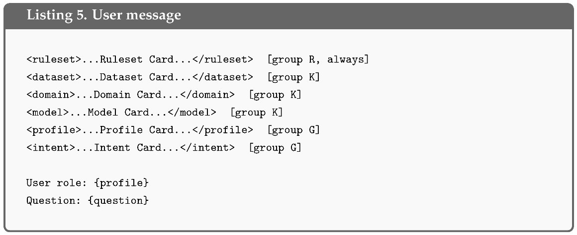
The cards are assembled in a fixed order so that a given configuration produces an identical prompt for every model. Generation is deterministic, so that any difference in output between configurations is attributable to the context and not to sampling. The decoding settings and hardware are reported in Section 4.6.
4. Experimental Setup
This section describes the case study, the construction of the rule surrogate, the question benchmark, the context configurations under comparison, the language models evaluated, and the protocol used to assess the generated explanations.
4.1. Case Study and Predictive Model
The experiments use the industrial injection moulding data introduced by Obregon et al. [1], collected from a moulding machine operating in a model factory in Singapore. Process-condition measurements were obtained from the machine controller and from external sensors, and the resulting parts were manually inspected for sink mark defects.
This study uses the dataset from Experiment 2 of the original work, in which the holding pressure and injection speed were varied in 25 configurations. The processed dataset contains 900 injection cycles, each representing one production instance, of which 613 are defective (class 0) and 287 are normal (class 1). The prediction task is therefore binary classification under moderate class imbalance.
The original data collection covered 30 categories of process-conditions related to temperature, force, speed, pressure, position, and processing time, several of which were recorded through multiple sensor channels or heating zones. In the processed representation used here, 38 individual time-series signals were retained, and eight statistical descriptors were extracted from each: maximum, minimum, mean, standard deviation, median, kurtosis, mean absolute deviation, and skewness. This yields predictive features per cycle. Feature names encode both the signal and the descriptor, so that Material_cushion_median denotes the median of the material cushion signal over the cycle. A complete description of the equipment, sensor placement, and data collection procedure is given in [1].
An XGBoost classifier [15] was used as the quality predictor. The dataset was divided once into training and test subsets by a 90/10 holdout split with a fixed random seed, giving 810 training instances (554 defective, 256 normal) and 90 test instances (59 defective, 31 normal). The objective of this study is not to optimise or comparatively evaluate the predictor. RuleSLM assumes that a sufficiently accurate tree ensemble is available and asks whether its decision logic can be transformed into rules that effectively ground natural language explanations. Accordingly, XGBoost was trained with its standard tree-booster configuration, using 100 trees and a maximum tree depth of 6, without task-specific hyperparameter tuning.
4.2. Rule Surrogate Construction
RuleCOSI+ [8] was applied to the trained ensemble to combine and simplify its tree-derived rules into an ordered decision list. The minimum rule-coverage threshold was set to 0, allowing low-coverage rules to remain eligible, and the minimum confidence threshold was set to 0.90. The resulting ruleset and its predictive performance are reported in Section 5.1.
Rule thresholds are displayed throughout the paper, and supplied to the generator, rounded to two decimal places. All predictive and fidelity metrics are computed on the exact extracted ruleset.
4.3. Question Benchmark
Explanation quality cannot be assessed without questions that exercise the distinct explanation goals the framework claims to serve. A benchmark of 58 questions was therefore constructed over the extracted ruleset, annotated with a stakeholder profile and a question intent, and paired with a curated reference answer.
Questions were systematically authored on the cross-product of the ruleset and the profile–intent taxonomy of Section 3.4. For each rule, questions were written that address the rule from the perspective of each stakeholder for whom that combination of rule and explanation goal is realistic. A further set of questions targets no single rule but requires aggregation across the decision list, for instance, comparing the evidence behind two rules or describing the order in which rules are evaluated. Five out-of-scope questions, unrelated to the process or the model, were included to test whether the generator respects the task boundary. Each question is annotated with the grounding source it draws on, which is either a single rule, a set of rules, or none in the out-of-scope case.
Table 3 reports the composition of the benchmark. The distribution follows the explanation goals that are realistic for each role, and is not a balanced factorial design. Operators receive no reliability assessment questions, since rule statistics fall outside their declared informational needs, and managers receive no rule summarisation questions. This is a property of the benchmark that constrains interpretation, and it is revisited in Section 6.5.
Table 3.
Composition of the question benchmark by stakeholder profile and question intent.
Of the 53 in-scope questions, 37 are grounded in a single rule, and 16 require aggregation across two or more rules. Reference answers average 48 words and respect the same five-sentence limit imposed on the generator, so that the generated and reference answers are comparable in length.
The complete benchmark, including the questions, stakeholder and intent annotations, rule annotations, evaluator grounding fields, and curated reference answers, is provided in Supplementary File S1.
Reference Answers
Each question is paired with a reference answer that states what a correct, role-appropriate response contains. Reference answers were drafted with a frontier large language model, ChatGPT-5.6 Sol with high effort, and then revised by the authors against the extracted ruleset and the contextual cards, correcting factual content, adjusting register to the target role, and enforcing the length constraint. The revised answers were fixed before any of the evaluated models were run, and no reference answer was modified at any later stage of the study.
Alongside each reference answer, the benchmark records the grounding evidence relevant to that question: the applicable rules, the pertinent dataset, domain, and model facts, and the profile and intent guidance. This evidence is supplied to the evaluator, as described in Section 4.7, and is never supplied to the generator beyond the cards active in the current configuration.
4.4. Context Configurations
The rule evidence group R is present in all configurations. Crossing the knowledge group K and the interaction guidance group G yields the four conditions of Table 4. Every model answers every question under every condition, giving generated explanations.
Table 4.
The four context configurations. Cards are those defined in Table 1.
4.5. Compared Small Language Models
Four open-weight instruction-tuned models from three families were evaluated, as summarised in Table 5. The selection spans the 1B–3B parameter range that is practical for on-premises deployment and includes two scales within one family, so that the effect of model size can be separated from the effect of model family. All models are used as released, without task-specific adaptation, so that the study measures the contribution of supplied context to an off-the-shelf model.
Table 5.
Small language models compared as RuleSLM generators. All are open-weight instruction-tuned variants, loaded from 4-bit quantised mirrors available on Hugging Face (https://huggingface.co, accessed on 25 March 2026).
4.6. Inference Environment
All experiments were conducted on a single NVIDIA RTX A5500 GPU with 23.54 GB of VRAM, running Linux 5.15 with Python 3.10.12 and CUDA 13.0. The software stack comprised PyTorch 2.11.0, Transformers 4.57.6, Unsloth 2026.8.9, and vLLM 0.20.0. Models were loaded in 4-bit quantisation with a maximum sequence length of 4608 tokens.
Generation used greedy decoding with a maximum of 512 new tokens and a repetition penalty of 1.2. Because decoding is deterministic, the canonical response for each model, condition, and question is produced once. Five warm-up requests precede each condition, and each response is additionally generated three times to characterise the dispersion of the latency and energy measurements, which vary with system state even when the output text does not. Determinism was verified by confirming that the three repetitions produced identical text in every case.
4.7. Evaluation Protocol
The evaluation of explanations is functionally grounded as explained in Section 2.5, and follows recommendations on automatic evaluation of generated text [36] in combining several complementary measures, each interpreted within its stated scope.
4.7.1. Rubric-Based Assessment
The primary measure is a rubric-based assessment performed by Prometheus 2 (7B) [16], an open evaluator model trained for scoring generated text against explicit criteria. Three rubrics are applied, each scoring a response from 1 to 5 on a criterion with written descriptors for every level:
- Grounding correctness. Whether the response is factually consistent with the authoritative evidence relevant to the question, including rule conditions, thresholds, predicted classes, and rule statistics, and whether it introduces unsupported claims. Predictive associations must not be presented as causal relationships.
- Relevance and completeness. Whether the response answers the specific question asked. Completeness is judged relative to the question, not to all available context, so a concise answer that fully addresses the request can receive the highest score.
- Role appropriateness. Whether the technical level, vocabulary, emphasis, and presentation suit the target role while remaining centred on the question. Role adaptation is assessed independently of factual correctness.
Each rubric receives only the evidence relevant to the property it assesses. Grounding correctness receives the applicable rules together with the dataset, domain, and model facts. Relevance and completeness receives the intent and its task requirement, while role appropriateness receives the stakeholder profile and the role-specific answer guidance. The evaluator receives the same evidence for a given question under every context configuration, including configurations in which the corresponding cards were withheld from the generator, and receives no indication of which model or configuration produced the response.
Each response is graded three times by the same evaluator model, once per rubric, in independent calls. A grading therefore has no access to the scores or the evidence of the other two dimensions, which is what allows a response to be judged factually correct and role-inappropriate at the same time.
The rubrics, the evidence routing, and the evaluator configuration were fixed before any of the evaluated models were run. Prometheus 2 (7B) was served through vLLM with a maximum context of 8192 tokens. All primary results reported in this paper, including the reference calibration of Section 4.7.2, use greedy decoding (temperature 0, top-p , maximum 1024 generated tokens, repetition penalty ). Greedy decoding selects the highest-probability token at every step, so evaluation is deterministic: repeated grading of the same response returns the same score and the same written feedback. The sensitivity analysis of Section 5.2 additionally reports two stochastic settings, which use the library defaults of temperature and top-p with the same token limit and repetition penalty.
4.7.2. Reference Calibration
A rubric score has no absolute interpretation on its own. To establish the attainable range of the instrument, the 58 curated reference answers were scored under the same three rubrics and the same evidence routing. This yields an upper anchor against which model scores can be read, and it also indicates which explanation goals are demanding for a careful human author. Because a reference answer cannot be compared against itself, the calibration pass scores each reference without a comparison answer, whereas model responses are scored against the corresponding reference. The two are therefore not identical measurements, and the calibration provides an anchor, not a directly comparable score. Reference answers were not revised in response to their calibration scores.
4.7.3. Evaluator Repeatability and Specification Sensitivity
An evaluator that is itself a language model is a measuring instrument, and its properties determine what the resulting scores can support. Two such properties are assessed directly.
The first is repeatability. Under stochastic decoding the evaluator returns a distribution of scores for a fixed response, and a single pass samples from it once. The magnitude of that variation is measured by scoring all 928 responses twice under identical stochastic settings and comparing the two passes: at the level of the individual grading and at the level of the configuration means that the analysis relies on.
The second is specification sensitivity. Rubric-based evaluation depends on choices that are not uniquely determined by the criteria being measured, in particular which evidence each rubric receives. All 928 responses were therefore scored under three evaluator settings: stochastic decoding, greedy decoding with the same rubric, and greedy decoding with the dimension-routed rubric specified in Section 4.7.1. Comparing the first two isolates the contribution of sampling, and comparing the second and third the contribution of the rubric specification. The third setting is used for all results reported in this paper; the first two are reported as a sensitivity analysis in Section 5.2.
4.7.4. Reference-Based and Auxiliary Measures
Reference-based similarity measures are reported alongside the rubrics: BERTScore [34] with RoBERTa-large embeddings; SBERT cosine similarity [35]; and the lexical overlap statistics BLEU [32], GLEU [39], and ROUGE [33]. Q2 [40] is applied to the in-scope questions as a measure of factual consistency with the rule evidence: candidate questions are generated from the response and answered independently against the response and against the grounding evidence, and the agreement between the two answers is aggregated. Perplexity under GPT-2 is reported as a descriptive indicator of surface fluency. None of these measures is interpreted as a measure of explanation quality in itself.
BERTScore, SBERT cosine similarity, ROUGE-L, and BLEU quantify lexical or embedding-level similarity to a reference text. Prometheus 2 evaluates responses against explicit criteria (Section 4.7.1): consistency with the supplied evidence, relevance and completeness for the question, and adaptation to the stakeholder role. We use rubric scores as the primary outcomes because they align with these evaluation objectives, with reference-based metrics as complementary measures. The measures show moderate positive correlations with the rubric mean across individual responses, although some configuration-level rankings differ (Section 5.6). The different rankings can reflect the evaluation targets of the measures. Reference-based metrics reward similarity to a particular answer, whereas the rubric explicitly assesses grounding, completeness, and role appropriateness. An explanation that changes its emphasis or adds relevant detail for a stakeholder may receive a higher rubric score without becoming more similar to the reference. A single reference also cannot represent every valid explanation. Conversely, the automated evaluator may favour particular presentation styles. These mechanisms could contribute to the observed disagreement, but the present analysis does not distinguish their contributions or establish which measure better reflects human judgement.
4.7.5. Deployment Measures
Because the framework targets on-premises inference, the cost of each configuration is measured directly on the hardware described in Section 4.6. Input and output token counts are recorded per response, latency and time to first token in seconds, generation throughput in output tokens per second, peak GPU memory and peak process resident memory in megabytes, average power draw in watts, and energy per response in joules. Power is sampled from the GPU at 50 ms intervals over the generation window, and energy is obtained by integrating the sampled power over that interval. Because these quantities vary with system state even when the generated text does not, each response is generated three times after five warm-up requests per configuration, and the reported values are means over the three repetitions.
Time to first token is reported separately from end-to-end latency, since the former reflects the cost of processing the supplied context while the latter also depends on how much text the model generates.
4.8. Statistical Analysis
The unit of analysis is the question. Generation is deterministic, so repeated inference for the same question, model, and configuration introduces no additional sampling variability. For each question, scores are averaged across the four models to give one value per question and condition, since model is a factor of interest and not a replicate, and configurations are compared by paired contrasts over the 58 matched questions. In each case, the null hypothesis is that the distribution of paired differences is symmetric about zero, and the alternative is that it is not.
Because the design is factorial, each context-group effect is observed twice, once with the other group absent and once with it present. A main effect is therefore estimated as the mean of those two simple effects, and the interaction as their difference. Applying these estimators to the dimensions each group is expected to affect yields the six contrasts of Table 6.
Table 6.
The six contrasts tested. Each is computed from the four context configurations of Table 4 and evaluated over the 58 matched questions. The two contrasts within RQ1 share an estimator, as do the two within RQ2, and differ only in the rubric dimension to which it is applied.
The analysis proceeds in three steps.
- 1.
- Omnibus test. A Friedman test over the four configurations establishes whether the configurations differ at all on a given dimension, which guards against interpreting pairwise differences in the absence of any overall effect.
- 2.
- Planned contrasts. Each of the six contrasts is tested with the Wilcoxon signed-rank test, using the matched-pairs rank-biserial correlation as the effect size and a percentile confidence interval for the mean difference from 10,000 question-level bootstrap resamples. The matched-pairs rank-biserial correlation compares the summed ranks of positive and negative question-level differences, indicating which direction dominates after accounting for their ranks. It complements the mean difference, which expresses the effect directly in rubric points. Within each research question, p-values are adjusted using the Holm procedure [41], and the null is rejected at the 5% level. This is the primary analysis.
- 3.
- Robustness checks. Two checks probe choices in the primary analysis that were not determined by the data. Applying the Holm correction across all six contrasts jointly tests sensitivity to the definition of the correction family used in the primary analysis. A cluster-level analysis first averages scores within each of the eight rule groups, so that each rule group contributes one observation. This tests sensitivity to treating the 58 questions as independent despite questions grounded in the same rule-sharing evidence. These checks assess whether the conclusions depend on the correction family or the unit of analysis; the cluster-level check also changes the weighting of the observations.
Results are therefore classified as established or suggestive. A contrast that is significant under the primary analysis and remains so under the omnibus test and both robustness checks is reported as an established effect. A contrast that is significant under the primary analysis but not under one or more of the checks is reported as suggestive, with the divergence stated. Per-model contrasts are reported separately where the aggregate conceals heterogeneity, using the Holm correction across the four models.
5. Results
5.1. Rule Surrogate
The trained XGBoost ensemble comprises 100 trees and yields 304 decision rules. RuleCOSI+ evaluated 112 rule combinations and reduced this to five conditional rules followed by one default rule, compressing the ensemble by a factor of approximately 50. Table 7 reports the resulting decision list.
Table 7.
The RuleCOSI+ ruleset extracted from the XGBoost ensemble, evaluated as an ordered decision list. Coverage, confidence, and the sample distribution are computed on the 810 training instances; the sample distribution is given as [defective, normal]. Thresholds are shown rounded to two decimal places, as supplied to the generator.
The five conditional rules identify normal parts and are stated over six process variables: dosage time, material cushion, mould heating circuit 3, screw volume, nozzle 1 pressure, and opening force. Material cushion appears in every conditional rule, and dosage time in the two with the widest coverage. The default rule assigns the remaining instances to the defective class and covers 68.40% of the training data. Rule alone accounts for 25.06% of training instances at perfect confidence, whereas covers a single instance. This spread is consequential for explanation, since a stakeholder asking how far a prediction can be trusted receives a very different answer depending on which rule fired.
Table 8 reports performance on the 90 held-out cycles. The ensemble classifies the test set without error. The extracted ruleset attains 97.78% accuracy, and because the ensemble is correct on every held-out instance, its fidelity to the ensemble is likewise 97.78%. The disagreement consists of two normal parts assigned to the defective class by the default rule.
Table 8.
Performance on the 90 held-out injection cycles. Fidelity is the proportion of held-out instances on which the surrogate and the ensemble produce the same prediction, as defined in Definition 1.
The held-out estimate is optimistic. The 900 cycles are sequential and adjacent cycles under a fixed machine configuration are highly correlated, so a random split does not fully separate training from test conditions. The predictive model is inherited from prior work and is not the object of this study.
The study varies the language models and supplied context while holding the predictive task and rule-based evidence fixed, enabling controlled comparisons between context configurations. Compact rule extraction is a design goal for RuleSLM, which targets small language models deployed on local hardware. The roughly 50-fold compression from 304 to 6 rules reflects this goal in the present case. The findings apply directly to this setting; whether the observed context effects persist with substantially larger or differently structured rulesets and other production processes remains an empirical question. The process data originate from sensor time series recorded during each production cycle. These signals are aggregated into per-cycle statistical descriptors (Section 4.1) to support tree-ensemble-based rule extraction. The framework therefore operates on time-series-derived features. Extending rule extraction to represent temporal trends or transitions directly is discussed in Section 7.
What matters here is that the ruleset stands in for the ensemble closely enough to serve as the evidential basis for the explanations evaluated below.
5.2. Evaluator Reliability and Sensitivity
Table 9 and Figure 2 report the agreement between two passes of the evaluator over all 928 responses under identical stochastic settings.
Table 9.
Agreement between two independent passes of the evaluator under identical stochastic settings, over 928 responses. QWK is the quadratic-weighted Cohen’s ; MAD is the mean absolute deviation in scale points.
Figure 2.
Repeatability of the evaluator across two passes under identical stochastic settings. (a) Paired role-appropriateness scores for 928 responses; cells show response counts. Exact agreement was 44%, with quadratic-weighted kappa of 0.504. (b) Configuration means for grounding correctness, relevance and completeness, and role appropriateness. Corresponding means differed by at most 0.12 points. Dashed lines indicate equal scores.
The two passes assign the same score to fewer than half of the individual gradings, and differ on average by roughly three quarters of a scale point (see Table 9). Agreement within one point is between 82% and 85%, and the disagreement is the mass lying off the diagonal in Figure 2a. A single rubric score for a single response is therefore not a reliable measurement.
The configuration means on which the analysis depends behave differently. Each is an average over 232 responses, corresponding to 58 questions answered by four models. Variation across individual gradings largely cancels under aggregation. No configuration mean differs between the two passes by more than 0.12 points on any single dimension or by more than 0.04 points on the mean of the three dimensions, despite individual gradings differing by 0.72 to 0.81 points on average. Figure 2b plots the two passes against one another at this level, and every point falls close to the identity line. Aggregate comparisons across configurations are stable even though the individual scores composing them are not. The analysis therefore uses paired aggregates, and the evaluator is operated deterministically.
Table 10 reports the three evaluator settings. Moving from stochastic to greedy decoding lowers scores on all three dimensions by 0.09 to 0.28 points. Sampling was inflating the measured quality of the responses, so the deterministic setting is both reproducible and more conservative.
Table 10.
Mean scores over all 928 responses under three evaluator settings. Deterministic 1 routes dimension-specific evidence as specified in Section 4.7.1. All results elsewhere in this paper use the Deterministic 2 setting.
The two deterministic settings are compared by a Wilcoxon signed-rank test over the 928 paired responses, each response scored once under each setting. This pairing is at the level of the individual response and is distinct from the analysis of Section 5.4, which pairs questions across generation configurations. Only relevance and completeness changes significantly, rising by 0.108 points (); this is the dimension whose evidence routing was altered. Grounding correctness and role appropriateness are statistically unchanged, at and . Individual gradings nevertheless move for approximately a quarter of responses on every dimension, including grounding correctness, whose routing is identical under both rubric versions. Rubric wording and evidence routing therefore both influence individual scores, and the two cannot be separated from this comparison.
The substantive conclusions reported below are largely unaffected by these settings. Every contrast estimated under the deterministic routed evaluator has the same sign as under the original stochastic evaluator, and the effect of interaction guidance on role appropriateness is significant under both, with a larger and more precisely determined estimate under the deterministic setting. One contrast changes status between the two evaluators, namely, the comparison of the full configuration against rule evidence alone; that contrast is examined under the full analysis in Section 5.4.
5.3. Calibration of the Evaluation Instrument
Table 11 reports the scores obtained by the 58 curated reference answers. These establish the attainable range of the instrument and are the scale against which the model scores are read.
Table 11.
Rubric scores of the curated reference answers, by question intent. Scores are on the 1–5 scale of Section 4.7.1.
The anchor is well below the top of the scale and differs by dimension, from 3.845 on grounding correctness to 4.690 on relevance and completeness (see Table 11). A model score is therefore interpreted against the anchor for its own dimension, and scores are not compared across dimensions, since the anchors reflect the strictness of each rubric as much as the difficulty of the property being measured.
The anchor also varies by explanation goal. Reliability assessment is the most demanding intent, scoring 3.409 on grounding correctness, which reflects the difficulty of stating coverage, confidence, and support precisely without overstating what training statistics establish. All five out-of-scope references score at the top of every rubric, confirming that the instrument correctly rewards a stated refusal when refusal is the intended behaviour.
Of the 58 references, 24 received a score below 4 on at least one dimension. Each was re-checked against the ruleset and the contextual cards and retained without modification.
5.4. Effect of Context on Explanation Quality
Table 12 reports the rubric scores by model and configuration together with the aggregate over the four models; Figure 3 plots that aggregate against the reference anchors; and Table 13 reports the statistical contrasts for the three research questions.
Table 12.
Rubric scores by model and context configuration. Each panel reports one dimension, with the reference anchor of Table 11 given in the panel heading. Panel headings and the ‘All models’ row are shown in italics; the ‘All models’ row is the average over the four models and is the aggregate on which the contrasts of Table 13 are computed. The best configuration for each model in the mean panel is shown in bold.
Figure 3.
Evaluator rubric scores by context configuration, averaged over four models and 58 questions: (a) grounding correctness; (b) relevance and completeness; (c) role appropriateness. Error bars are 95% percentile bootstrap intervals over questions. Dashed lines show mean reference-answer scores (Table 11). Blue bars identify configurations containing interaction guidance in panel (c); its planned main effect was +0.323 points (Holm-adjusted ).
Table 13.
Paired contrasts over the 58 matched questions. Effect size is the matched-pairs rank-biserial correlation; intervals are 95% percentile bootstrap intervals from 10,000 resamples; p-values are Holm-adjusted within each research question.
- RQ1. Does knowledge context improve the factual grounding and completeness of generated explanations?
Supplying the dataset, domain, and model cards produces no detectable change in either grounding correctness or relevance and completeness. Both estimates lie within 0.03 points of zero, and their confidence intervals exclude any improvement larger than roughly a tenth of a rubric point (see Table 13). The aggregate null nevertheless masks some model-specific variation. On grounding correctness, the two smallest models decline under knowledge context, with Qwen2.5-1.5B falling from 3.000 to 2.638 and Gemma-2-2B from 3.017 to 2.672, while Llama-3.2-3B rises from 3.276 to 3.414 (see Table 12). Grounding correctness is also the weakest dimension in absolute terms under every configuration, reaching at most 2.914 against an anchor of 3.845, so the absence of an effect is not attributable to a ceiling.
- RQ2. Does interaction guidance improve the appropriateness of explanations for the target role?
Supplying the profile and intent cards increases the evaluator’s role appropriateness score by 0.323 points (see Table 13), with a rank-biserial correlation of 0.683 indicating a strong predominance of positive differences across questions. This is the only dimension in Figure 3 in which the bars rise across the four configurations. No statistically detectable average change is observed in relevance or grounding. The two context groups act on different properties of the explanation, and the property guidance acts on is the one it was designed to address. Excluding the five out-of-scope questions, for which the guidance carries an explicit refusal instruction, the effect remains at with .
To examine sensitivity to the benchmark’s role–intent composition, we repeated the G-on-role-appropriateness analysis on the 23 process-diagnostics questions, the only in-scope intent represented across all three roles (Table 3). The estimated effect is +0.272 rubric points (rank-biserial correlation 0.630; 95% confidence interval for the mean effect [0.114, 0.446]; unadjusted p = 0.008), compared with +0.323 in the full sample. This exploratory check uses a two-sided Wilcoxon signed-rank test with the normal approximation, average ranks for ties, and no continuity correction. The percentile confidence interval uses 10,000 question-level bootstrap resamples (seed 0). This provides evidence of a positive effect within a shared intent, but the subset retains unequal role counts (fourteen operator, four manager, and five data-scientist questions) and different question content. It therefore does not establish equal benefits across roles or address the missing role–intent combinations. Moreover, G supplies profile and intent guidance jointly, so their individual contributions remain unresolved.
The improvement comes largely from responses leaving the lowest score band: as Figure 4 shows, the number of responses scoring 1 on role appropriateness falls from 61 under rule evidence alone to 37 under the full configuration.
Figure 4.
Distribution of role-appropriateness scores by context configuration. Each bar contains 232 responses (58 questions answered by four models). The number scoring 1 falls from 61 under R to 37 under R + K + G, a reduction of approximately 39%.
- RQ3. Do knowledge context and interaction guidance interact, and is any such interaction consistent across model families and scales?
The aggregate interaction between the two groups is positive but not significant. The full-context versus rule-only contrast is positive (+0.175 rubric points) and significant under the primary analysis (Holm-adjusted p = 0.021). Its adjusted p-value increases to 0.052 when correction is applied across all six contrasts. Aggregating the 58 questions into eight rule groups and giving each group equal weight yields a positive estimate of +0.216 points (p = 0.055). This check reduces the number of analysis units and changes the weighting of the observations; the present analysis does not quantify how much each contributes to the change in significance. The Friedman omnibus test assesses an overall configuration effect across all four conditions, while the planned contrast targets the full-context versus rule-only comparison; their significance decisions need not coincide. Nevertheless, the omnibus result (p = 0.355) and the two robustness checks do not meet our stated criteria for an established effect (Table 14). We therefore retain the classification as suggestive. The effect of interaction guidance on role appropriateness, by contrast, is established because it survives every check applied. The aggregate interaction additionally conceals two significant and opposing model-level interactions, which the next subsection examines.
Table 14.
The two contrasts that are significant under the primary analysis, evaluated under the omnibus test and the two robustness checks of Section 4.8. A contrast is reported as established only if it survives all four.
5.5. Model-Specific Behaviour
No ordering of configurations holds across all four models, and the best configuration differs by model (see the mean panel of Table 12). Table 15 and Figure 5 report the per-model interaction and the per-model effect of guidance on role appropriateness. Two models show a significant interaction, and the two have opposite signs. The per-model effects of knowledge context were tested on the same basis and were null in every model.
Table 15.
Per-model contrasts. p-values are Holm-adjusted across the four models within each contrast. Values in bold are significant at the 5% level.
Figure 5.
Interaction between knowledge context (K) and interaction guidance (G) by model: (a) Llama-3.2-1B; (b) Qwen2.5-1.5B; (c) Gemma-2-2B; (d) Llama-3.2-3B. Points show scores averaged across the three rubric dimensions and 58 questions. Blue indicates a significant interaction in the primary analysis (Table 15); grey indicates a non-significant interaction. The diverging lines in (c) indicate a complementary interaction; the converging lines in (d) indicate a substitutive interaction. All panels share the same vertical scale.
For Llama-3.2-3B the two context groups act as substitutes. Guidance added to rule evidence alone raises the mean score from 3.402 to 3.649, a gain of 0.247 points, whereas guidance added when knowledge context is already present raises it from 3.649 to 3.661 (see lower panel, ‘Mean of the three dimensions’, in Table 12). Either group alone brings the model to 3.649 and supplying both adds nothing further, which is the convergence visible in panel (d) of Figure 5. This is the strongest model in the comparison, and it extracts from either context group whatever the other would have provided. Its highest role appropriateness score, 3.914, is reached under interaction guidance alone and not under the full configuration.
For Gemma-2-2B the two groups act as complements. Guidance added to rule evidence alone moves the mean from 3.109 to 3.264, a gain of 0.155 points, against 0.747 when it is added in the presence of knowledge context (from 2.621 to 3.368). The reason is that knowledge context alone degrades this model sharply, from 3.109 to 2.621, with role appropriateness falling from 2.690 to 2.138, the lowest value recorded anywhere in the study (see Table 12). Interaction guidance is what prevents that degradation, and the two lines in Figure 5 diverge accordingly.
The mechanism is visible in the generated text and in the output token counts reported in Section 5.7. Under knowledge context, Gemma-2-2B does not become less accurate. It becomes concise. Its mean output length falls from 64.6 tokens under rule evidence alone to 41.6 under R + K, recovering to 60.5 when guidance is restored. Answers collapse into fragments that are factually correct but insufficient as explanations, such as returning the bare figure 256 in response to a question about how much training evidence supports a rule. Knowledge context shifts the model from explanation toward fact retrieval, while interaction guidance restores the explanatory register. No other model shows this pattern. Output length rises under knowledge context for the remaining three models, including from 96.8 to 129.8 tokens for Llama-3.2-3B and from 97.7 to 128.6 for Qwen2.5-1.5B (see Section 5.7).
Twenty responses reached the 512-token generation limit: nineteen of them from Llama-3.2-1B, distributed across all four configurations; and one from Qwen2.5-1.5B under R + K.
5.6. Complementary Measures
Table 16 reports the reference-based and auxiliary measures, which separate the configurations weakly and in a manner inconsistent with the rubric scores.
Table 16.
Complementary measures by context configuration, averaged over models and questions. Q2 is computed on the 53 in-scope questions.
BERTScore and ROUGE-L rank rule evidence alone highest and the full configuration lowest. SBERT and BLEU instead rank R + G highest and R + K lowest. These rankings differ in part from the rubric ordering. Across individual responses, the rubric mean correlates positively with the four reference-based measures (–), so differences between configuration rankings do not imply inverse response-level correlations. Differences in the evaluation targets, the range of valid explanations, and possible evaluator preferences may contribute to this pattern, as discussed in Section 4.7.4; the present analysis does not establish their respective contributions. Q2 and perplexity have little association with the rubric mean (see Table 16) and are retained as complementary descriptive measures.
5.7. Deployment Cost of Context
Table 17 reports the inference cost of each configuration by model on the single-GPU environment of Section 4.6, and Figure 6 decomposes the aggregate.
Table 17.
Inference cost by model and context configuration. Time to first token reflects the cost of processing the supplied context; end-to-end latency additionally depends on the length of the generated response. Panel headings and the ‘All models’ row are shown in italics; the ‘All models’ row is the average over the four models.
Figure 6.
Computational cost by context configuration, averaged over questions and models. (a) End-to-end latency separated into time to first token and subsequent generation time. (b) Input tokens decomposed into the rule-evidence baseline (R) and additional knowledge (K) and guidance (G) components. Full context increases time to first token by approximately 239% relative to R alone.
Moving from rule evidence alone to the full configuration increases input length by 275%, time to first token by 239%, peak GPU memory by 21%, and energy per response by 50% (see Table 17). End-to-end latency increases by 38%, but this figure combines two costs. Time to first token isolates the cost of processing the supplied context and scales with prompt length. The remainder depends on how much text the model generates, which also grows with context, from 120.1 to 146.8 output tokens on average. Panel (a) of Figure 6 separates the two components, and panel (b) attributes the prompt growth to each context group. Configurations that elicit longer answers are therefore penalised twice in end-to-end latency, and the isolated cost of context is better read from time to first token.
Interaction guidance is the cheaper of the two additions. It adds 999 input tokens against 1452 for knowledge context, and 51 J against 101 J per response, while producing the only context effect that holds across the question set.
The cost of a given configuration is not the same for every model. Identical prompts are tokenised differently across families, so rule evidence alone occupies 856 tokens for both Llama models, 897 for Qwen2.5-1.5B, and 953 for Gemma-2-2B, with similar proportional differences under every configuration. Gemma-2-2B is also the only model whose end-to-end latency falls under knowledge context, from 1.20 to 0.96 s. This reduction follows from the shortening of its outputs; its time to first token rises over the same comparison from 0.09 to 0.25 s. Peak GPU memory varies primarily with model size, ranging from 1.4 GB for Llama-3.2-1B to 3.0 GB for Llama-3.2-3B under the full configuration, so all four models remain deployable on a single workstation GPU under every configuration tested.
5.8. Qualitative Comparison
Table 18 contrasts two responses to questions about the same rule, addressed to the same stakeholder role and generated under the same configuration, at opposite ends of the score range.
Table 18.
Two responses grounded in rule , both addressed to an operator and generated under R + K + G. Evaluator feedback is abridged.
The two cases illustrate what the rubrics separate. The high-scoring response states every condition with exact thresholds and stops there, losing a point on role appropriateness only because it leaves the statistical suffixes untranslated, which the operator profile requires. The low-scoring response fails on all three dimensions for the same underlying reason: it answers a question that was not asked. The weakest model produced this response under the full configuration, consistent with the aggregate finding that additional context does not compensate for the limited model capability.
6. Discussion
6.1. Context Should Be Selected, Not Supplied in Full
The results contradict the assumption that grounding a compact language model in all available context produces better explanations. Interaction guidance increases the evaluator’s role-appropriateness score at lower cost. Knowledge context produces no statistically detectable average change in the grounding-correctness or relevance-and-completeness scores.
The specificity of the effects is what makes the decomposition useful. Interaction guidance increased the evaluator’s role-appropriateness score, with no statistically detectable average change in the other two dimensions. Knowledge context produced no measurable average change. Each group therefore acts, at most, on the property it was designed to address, and supplying a group does not produce diffuse improvement across the explanation. A practitioner assembling such a system can select context according to the property that needs improving and omit components associated with properties that are already adequate.
The results also indicate where the difficulty in this task lies. Grounding correctness is the weakest dimension under every configuration, and no context configuration improves it. Explanations that misreport a threshold or overstate what a rule’s confidence establishes are not corrected by supplying more description of the process or the dataset. The evidence needed to answer these questions was present in the ruleset under every configuration, so the problem lies in using available rule evidence, not in missing contextual information. Additional context therefore does not address it.
6.2. Context Requirements Depend on Model Capability
The aggregate interaction between the two groups hides two significant model-level interactions with opposite signs. On the strongest model, the groups substitute for one another, since either alone achieves what both together achieve. On Gemma-2-2B, they complement one another because knowledge context alone degrades the model, and interaction guidance prevents the degradation.
Under knowledge context, Gemma-2-2B does not hallucinate or misreport rules. Instead, it produces shorter answers that remain factually defensible but are insufficient as explanations. The knowledge cards appear to shift the model towards a fact-retrieval register, while the profile and intent cards restore the explanatory one. The other three models lengthen their outputs under the same cards, so this pattern is specific to Gemma-2-2B in the present experiment.
A possible explanation is model capability. A stronger model may obtain what it needs from either group, while a weaker one may require guidance to maintain the intended explanatory register. The present design cannot establish this because each interaction direction rests on a single model. The comparison includes one Qwen model (Qwen2.5-1.5B), one Gemma model (Gemma-2-2B), and two Llama models (Llama-3.2-1B and Llama-3.2-3B). It therefore provides only one within-family size comparison and does not independently separate family, parameter count, and other checkpoint-specific characteristics. The significant complementary interaction for Gemma-2-2B and substitutive interaction for Llama-3.2-3B describe the tested models; their underlying causes cannot be distinguished with the present design. The per-model grounding scores of Table 12 complicate the interpretation further. Knowledge context lowers grounding correctness on both models below 2B and raises it only on the largest. The results do establish a practical consequence. A context configuration validated on one model does not necessarily transfer to another, and the configuration to be deployed must be determined on the model that will run it.
6.3. What the Evaluator Supports, and What It Does Not
The repeatability analysis of Section 5.2 has implications beyond this study. Systems that filter or re-rank generated explanations using an automatic evaluator of this kind rely on a per-response signal that is not stable across repeated grading, even though the same instrument supports stable comparisons between configurations. The conclusions above are therefore stated as comparisons between configurations and not as absolute quality levels. Scores from this evaluator should not be used to select outputs at inference time.
6.4. Deployment Implications
The framework targets on-premises inference on a single workstation GPU, where context cost is a deployment constraint. As Figure 7 shows, the highest-scoring configuration is not the most efficient one for any model. The clearest illustration is Llama-3.2-3B, which scores 3.649 at 348 J per response under interaction guidance and 3.661 at 590 J under the full configuration (see Table 12 and Table 17). This represents approximately 70% greater energy use for about 0.01 additional rubric points. Under continuous deployment, this difference accumulates across requests and would be missed by an evaluation reporting quality alone.
Figure 7.
Mean evaluator rubric score versus energy per response. Colours identify models; marker shapes identify context configurations. Scores are averaged over the three rubric dimensions and 58 questions. The arrow connects R + G and R + K + G for Llama-3.2-3B, showing approximately 70% greater energy use for about 0.01 additional rubric points.
Cost is also not evenly distributed across models. Because tokenisation differs between families, the same contextual cards occupy about 11% more of the prompt budget on Gemma-2-2B than on either Llama model, and that overhead is paid on every request for the lifetime of the deployment. Token counts measured for one model therefore do not transfer directly to another.
Two further observations concern the limits of prompt-level instructions. The Intent card specifies the required response to an out-of-scope request, yet refusal rates neither exceeded 55% nor improved when the card was supplied. Internal context tags or labels appeared in 8.08% of responses (75 of 928) despite an explicit prohibition in the system prompt. The rate was 17.24% for Llama-3.2-1B and 2.59% for Llama-3.2-3B; it was 11.21% under R+K and 4.74% under R+G. These findings indicate that prompt instructions alone do not enforce the requested behaviour. Deployment therefore requires boundary checks and output validation independent of the generator. A post-processing filter could detect and remove isolated internal tags where this preserves the answer’s meaning. Cases in which internal labels are embedded in the explanation require further review or regeneration. Targeted instruction-following fine-tuning or constrained decoding could also be investigated. The effectiveness of these proposed measures remains to be evaluated.
6.5. Limitations
The evaluation is functionally grounded, but Prometheus 2 was not compared against human experts in this study. The results therefore establish that configurations differ under a fixed and calibrated instrument, not that the differences correspond to differences in usefulness for operators, managers, or data scientists. The repeatability analysis assesses the instrument’s consistency but does not establish its validity.
The controlled comparison holds the predictive task and rule evidence fixed while varying the language model and supplied context. Its findings apply directly to this setting. Transfer to other production processes or substantially larger and differently structured rulesets remains an empirical question.
Stakeholder profile and question intent are not fully crossed in the benchmark, and the interaction guidance group bundles the profile and intent cards. The effect of guidance on role appropriateness therefore cannot be attributed to the profile card specifically, and the design does not separate adaptation to the reader from adaptation to the question. The process-diagnostics sensitivity check in Section 5.4 restricts the comparison to a shared intent, but retains unequal role counts and different question content. It therefore does not resolve the missing role–intent combinations or establish equal benefits across roles.
Finally, the predictive model is inherited from prior work and its held-out performance is estimated from a random split of sequential production cycles. This does not affect the comparison of context configurations, all of which are grounded in the same ruleset, but the reported accuracy and fidelity should not be read as estimates of field performance.
7. Conclusions and Future Work
This study addressed the step between an interpretable surrogate model and an explanation that a stakeholder can act on. RuleSLM extracts a compact ruleset from a tree ensemble trained to predict sink mark defects in injection moulding, and grounds a locally deployed small language model in that ruleset together with structured context inputs, producing explanations addressed to operators, production managers, and data scientists. The framework makes it possible to examine which context a compact model needs and the cost of supplying it.
Decomposing the supplied context into rule evidence, knowledge, and interaction guidance, and crossing the latter two in a factorial design over four small language models and 58 role- and intent-annotated questions, answers the three research questions as follows. Knowledge context produces no statistically detectable average change in grounding correctness or relevance and completeness, while increasing input length substantially. Interaction guidance increases the evaluator’s role-appropriateness score by 0.323 points, with a large rank-biserial effect size and no statistically detectable average change in the other dimensions. The two groups interact in opposite directions on two different models, substituting for one another on the strongest model and complementing one another on a model that degrades under knowledge context alone. Supplying the full context increases input length by 275% and energy per response by 50%, for a benefit confined to one of the three quality dimensions and not robust to every correction applied.
The practical consequence is that context for rule-grounded explanation should be selected for the property it serves and validated on the model that will be deployed, since no configuration was best for all four models and the two significant interactions had opposite signs.
The work presented herein has some limitations, as set out in Section 6.5. The most consequential is that the evaluator was calibrated against curated reference answers but never validated against human experts, so the results establish that configurations differ under a fixed instrument and not that they differ in usefulness to the stakeholders addressed.
As future work, the most direct extension is expert human evaluation. Establishing whether the judgements of an automatic evaluator correspond to those of manufacturing practitioners requires domain experts to score the same responses under the same rubrics. This would allow the comparative findings reported here to be assessed in terms of stakeholder usefulness. A second direction concerns the content of the context itself. The rules used here express predictive associations, and the evaluation protocol explicitly penalizes explanations that present them as causal. Contextual cards that encode the causal structure of the process variables could support interventional questions such as which setting to change and in which direction. Another direction is to extend rule extraction and rule-grounded explanation to represent temporal structure directly, including trends or transitions within a production cycle. A further direction is to test multiple models within each family at matched parameter scales to investigate whether the observed K × G interactions reflect model family, scale, or other model-specific characteristics.
Supplementary Materials
The following supporting information can be downloaded at https://www.mdpi.com/article/10.3390/pr14193158/s1: File S1: RuleSLM experimental materials, including the six contextual cards used in the experiments, the 58-question benchmark with curated reference answers, the generation prompt and user-message template, the Prometheus rubric configurations and evaluator metadata, reference-answer calibration scores, response-level results for all 928 generated explanations, and response-level scores for the evaluator sensitivity settings.
Author Contributions
Conceptualization, J.J.R. and J.O.; methodology, J.J.R. and J.O.; software, J.J.R.; validation, J.J.R. and J.O.; formal analysis, J.J.R.; investigation, J.J.R.; resources, J.O.; data curation, J.J.R.; writing—original draft preparation, J.J.R.; writing—review and editing, J.O.; visualization, J.J.R.; supervision, J.O.; project administration, J.O.; funding acquisition, J.O. All authors have read and agreed to the published version of the manuscript.
Funding
This study was financially supported by Seoul National University of Science & Technology.
Data Availability Statement
The underlying injection-moulding process data are not publicly available due to confidentiality and contractual restrictions imposed by the data provider. The contextual cards, question benchmark, generation prompt, evaluator specifications, reference-answer scores, and response-level experimental results generated in this study are provided in the Supplementary Materials.
Acknowledgments
During the preparation of the question benchmark, a large language model was used to draft candidate reference answers, which were subsequently revised and verified by the authors against the extracted rule set and the contextual cards. Additionally, during the preparation of this manuscript, the authors used ChatGPT-5.6 Sol and Claude Opus 5 for the purposes of reviewing the quality and correctness of the code used in the experiments, checking the statistical analyses, and improving the clarity and structure of the manuscript. The authors have reviewed and edited the outputs and take full responsibility for the content of this publication.
Conflicts of Interest
The authors declare no conflicts of interest.
References
- Obregon, J.; Hong, J.; Jung, J.Y. Rule-based explanations based on ensemble machine learning for detecting sink mark defects in the injection moulding process. J. Manuf. Syst. 2021, 60, 392–405. [Google Scholar] [CrossRef] [Scilit]
- Obregon, J.; Jung, J.Y. Rule-based visualization of faulty process conditions in the die-casting manufacturing. J. Intell. Manuf. 2024, 35, 521–537. [Google Scholar] [CrossRef] [Scilit]
- Çınar, Z.M.; Abdussalam Nuhu, A.; Zeeshan, Q.; Korhan, O.; Asmael, M.; Safaei, B. Machine Learning in Predictive Maintenance towards Sustainable Smart Manufacturing in Industry 4.0. Sustainability 2020, 12, 8211. [Google Scholar] [CrossRef] [Scilit]
- Ko, J.H.; Yin, C. A review of artificial intelligence application for machining surface quality prediction: From key factors to model development. J. Intell. Manuf. 2026, 37, 775–798. [Google Scholar] [CrossRef] [Scilit]
- Barredo Arrieta, A.; Díaz-Rodríguez, N.; Del Ser, J.; Bennetot, A.; Tabik, S.; Barbado, A.; Garcia, S.; Gil-Lopez, S.; Molina, D.; Benjamins, R.; et al. Explainable Artificial Intelligence (XAI): Concepts, taxonomies, opportunities and challenges toward responsible AI. Inf. Fusion 2020, 58, 82–115. [Google Scholar] [CrossRef] [Scilit]
- Puthanveettil Madathil, A.; Luo, X.; Liu, Q.; Walker, C.; Madarkar, R.; Qin, Y. A review of explainable artificial intelligence in smart manufacturing. Int. J. Prod. Res. 2025, 63, 8654–8697. [Google Scholar] [CrossRef] [Scilit]
- Nikiforidis, K.; Kyrtsoglou, A.; Vafeiadis, T.; Kotsiopoulos, T.; Nizamis, A.; Ioannidis, D.; Votis, K.; Tzovaras, D.; Sarigiannidis, P. Enhancing transparency and trust in AI-powered manufacturing: A survey of explainable AI (XAI) applications in smart manufacturing in the era of industry 4.0/5.0. ICT Express 2025, 11, 135–148. [Google Scholar] [CrossRef] [Scilit]
- Obregon, J.; Jung, J.Y. RuleCOSI+: Rule extraction for interpreting classification tree ensembles. Inf. Fusion 2023, 89, 355–381. [Google Scholar] [CrossRef] [Scilit]
- Du, K.; Yang, B.; Xie, K.; Dong, N.; Zhang, Z.; Wang, S.; Mo, F. LLM-MANUF: An integrated framework of Fine-Tuning large language models for intelligent Decision-Making in manufacturing. Adv. Eng. Inform. 2025, 65, 103263. [Google Scholar] [CrossRef] [Scilit]
- Ding, D.; Mallick, A.; Wang, C.; Sim, R.; Mukherjee, S.; Rühle, V.; Lakshmanan, L.; Awadallah, A.H. Hybrid llm: Cost-efficient and quality-aware query routing. In Proceedings of the International Conference on Learning Representations, Vienna, Austria, 7–11 May 2024; Volume 2024, pp. 41348–41366. [Google Scholar]
- Lu, Z.; Li, X.; Cai, D.; Yi, R.; Liu, F.; Zhang, X.; Lane, N.D.; Xu, M. Small Language Models: Survey, Measurements, and Insights. arXiv 2025, arXiv:2409.15790. [Google Scholar] [CrossRef] [Scilit]
- Grattafiori, A.; Dubey, A.; Jauhri, A.; Pandey, A.; Kadian, A.; Al-Dahle, A.; Letman, A.; Mathur, A.; Schelten, A.; Vaughan, A.; et al. The Llama 3 Herd of Models. arXiv 2024, arXiv:2407.21783. [Google Scholar] [CrossRef] [Scilit]
- Yang, A.; Yang, B.; Zhang, B.; Hui, B.; Zheng, B.; Yu, B.; Li, C.; Liu, D.; Huang, F.; Wei, H.; et al. Qwen2.5 Technical Report. arXiv 2025, arXiv:2412.15115. [Google Scholar] [CrossRef] [Scilit]
- Team, G.; Riviere, M.; Pathak, S.; Sessa, P.G.; Hardin, C.; Bhupatiraju, S.; Hussenot, L.; Mesnard, T.; Shahriari, B.; Ramé, A.; et al. Gemma 2: Improving Open Language Models at a Practical Size. arXiv 2024, arXiv:2408.00118. [Google Scholar] [CrossRef] [Scilit]
- Chen, T.; Guestrin, C. XGBoost: A Scalable Tree Boosting System. In Proceedings of the 22nd ACM SIGKDD International Conference on Knowledge Discovery and Data Mining, San Francisco, CA, USA, 13–17 August 2016; pp. 785–794. [Google Scholar] [CrossRef] [Scilit]
- Kim, S.; Suk, J.; Longpre, S.; Lin, B.Y.; Shin, J.; Welleck, S.; Neubig, G.; Lee, M.; Lee, K.; Seo, M. Prometheus 2: An Open Source Language Model Specialized in Evaluating Other Language Models. In Proceedings of the 2024 Conference on Empirical Methods in Natural Language Processing; Association for Computational Linguistics: Kerrville, TX, USA, 2024; pp. 4334–4353. [Google Scholar] [CrossRef] [Scilit]
- Lin, C.Y.; Gim, J.; Shotwell, D.; Lin, M.T.; Liu, J.H.; Turng, L.S. Explainable artificial intelligence and multi-stage transfer learning for injection molding quality prediction. J. Intell. Manuf. 2025, 36, 3587–3606. [Google Scholar] [CrossRef] [Scilit]
- Silva, B.; Marques, R.; Faustino, D.; Ilheu, P.; Santos, T.; Sousa, J.; Rocha, A.D. Enhance the Injection Molding Quality Prediction with Artificial Intelligence to Reach Zero-Defect Manufacturing. Processes 2022, 11, 62. [Google Scholar] [CrossRef] [Scilit]
- Jun, J.h.; Chang, T.W.; Jun, S. Quality Prediction and Yield Improvement in Process Manufacturing Based on Data Analytics. Processes 2020, 8, 1068. [Google Scholar] [CrossRef] [Scilit]
- Deng, X.; Xiang, W.; Lin, W.; Zheng, Z.; Yang, Y. Few-shot injection molding quality prediction method integrating deep transfer and multi-task learning. Int. J. Adv. Manuf. Technol. 2025, 141, 609–632. [Google Scholar] [CrossRef] [Scilit]
- Adadi, A.; Berrada, M. Peeking Inside the Black-Box: A Survey on Explainable Artificial Intelligence (XAI). IEEE Access 2018, 6, 52138–52160. [Google Scholar] [CrossRef] [Scilit]
- Moosavi, S.; Farajzadeh-Zanjani, M.; Razavi-Far, R.; Palade, V.; Saif, M. Explainable AI in Manufacturing and Industrial Cyber–Physical Systems: A Survey. Electronics 2024, 13, 3497. [Google Scholar] [CrossRef] [Scilit]
- Wang, C.C.; Chien, C.H. Machine Learning for Industrial Optimization and Predictive Control: A Patent-Based Perspective with a Focus on Taiwan’s High-Tech Manufacturing. Processes 2025, 13, 2256. [Google Scholar] [CrossRef] [Scilit]
- Longo, L.; Brcic, M.; Cabitza, F.; Choi, J.; Confalonieri, R.; Ser, J.D.; Guidotti, R.; Hayashi, Y.; Herrera, F.; Holzinger, A.; et al. Explainable Artificial Intelligence (XAI) 2.0: A manifesto of open challenges and interdisciplinary research directions. Inf. Fusion 2024, 106, 102301. [Google Scholar] [CrossRef] [Scilit]
- Friedman, J.H.; Popescu, B.E. Predictive Learning via Rule Ensembles. Ann. Appl. Stat. 2008, 2, 916–954. [Google Scholar] [CrossRef] [Scilit]
- Deng, H. Interpreting Tree Ensembles with inTrees. Int. J. Data Sci. Anal. 2019, 7, 277–287. [Google Scholar] [CrossRef] [Scilit]
- Liu, B.; Mazumder, R. Fire: An Optimization Approach for Fast Interpretable Rule Extraction. In Proceedings of the 29th ACM SIGKDD Conference on Knowledge Discovery and Data Mining; ACM: New York, NY, USA, 2023; pp. 1396–1405. [Google Scholar] [CrossRef] [Scilit]
- Bonasera, L.; Carrizosa, E. A unified approach to extract interpretable rules from tree ensembles via integer programming. Comput. Oper. Res. 2025, 185, 107283. [Google Scholar] [CrossRef] [Scilit]
- Lu, Z.; Li, X.; Cai, D.; Yi, R.; Liu, F.; Liu, W.; Luan, J.; Zhang, X.; Lane, N.D.; Xu, M. Demystifying Small Language Models for Edge Deployment. In Proceedings of the 63rd Annual Meeting of the Association for Computational Linguistics; Association for Computational Linguistics: Kerrville, TX, USA, 2025; Volume 1: Long Papers, pp. 14747–14764. [Google Scholar] [CrossRef] [Scilit]
- Lewis, P.; Perez, E.; Piktus, A.; Petroni, F.; Karpukhin, V.; Goyal, N.; Kuettler, H.; Lewis, M.; Yih, W.t.; Rocktaeschel, T.; et al. Retrieval-Augmented Generation for Knowledge-Intensive NLP Tasks. In Proceedings of the Advances in Neural Information Processing Systems, Virtual, 6–12 December 2020; Volume 33, pp. 9459–9474. [Google Scholar]
- Doshi-Velez, F.; Kim, B. Considerations for Evaluation and Generalization in Interpretable Machine Learning. In The Springer Series on Challenges in Machine Learning; Springer International Publishing: Cham, Switzerland, 2018; pp. 3–17. [Google Scholar] [CrossRef] [Scilit]
- Papineni, K.; Roukos, S.; Ward, T.; Zhu, W.J. Bleu: A method for automatic evaluation of machine translation. In Proceedings of the 40th Annual Meeting of the Association for Computational Linguistics, Philadelphia, PA, USA, 6–12 July 2002; pp. 311–318. [Google Scholar]
- Lin, C.Y. Rouge: A package for automatic evaluation of summaries. In Proceedings of the Text Summarization Branches Out, Barcelona, Spain, 25–26 July 2004; pp. 74–81. [Google Scholar]
- Zhang, T.; Kishore, V.; Wu, F.; Weinberger, K.Q.; Artzi, Y. BERTScore: Evaluating Text Generation with BERT. arXiv 2020, arXiv:1904.09675. [Google Scholar] [CrossRef] [Scilit]
- Reimers, N.; Gurevych, I. Sentence-BERT: Sentence Embeddings using Siamese BERT-Networks. In Proceedings of the 2019 Conference on Empirical Methods in Natural Language Processing and the 9th International Joint Conference on Natural Language Processing (EMNLP-IJCNLP); Association for Computational Linguistics: Kerrville, TX, USA, 2019; pp. 3980–3990. [Google Scholar] [CrossRef] [Scilit]
- Schmidtova, P.; Mahamood, S.; Balloccu, S.; Dusek, O.; Gatt, A.; Gkatzia, D.; Howcroft, D.M.; Platek, O.; Sivaprasad, A. Automatic Metrics in Natural Language Generation: A survey of Current Evaluation Practices. In Proceedings of the 17th International Natural Language Generation Conference; Association for Computational Linguistics: Kerrville, TX, USA, 2024; pp. 557–583. [Google Scholar] [CrossRef] [Scilit]
- Zheng, L.; Chiang, W.L.; Sheng, Y.; Zhuang, S.; Wu, Z.; Zhuang, Y.; Lin, Z.; Li, Z.; Li, D.; Xing, E.; et al. Judging llm-as-a-judge with mt-bench and chatbot arena. Adv. Neural Inf. Process. Syst. 2023, 36, 46595–46623. [Google Scholar] [CrossRef] [Scilit]
- Khoo, T.L.; Lee, T.S.; Bee, S.T.; Ma, C.; Zhang, Y.Y. A Comparative Review of Large Language Models in Engineering with Emphasis on Chemical Engineering Applications. Processes 2025, 13, 2680. [Google Scholar] [CrossRef] [Scilit]
- Napoles, C.; Sakaguchi, K.; Post, M.; Tetreault, J. GLEU Without Tuning. arXiv 2016, arXiv:1605.02592. [Google Scholar] [CrossRef] [Scilit]
- Honovich, O.; Choshen, L.; Aharoni, R.; Neeman, E.; Szpektor, I.; Abend, O. Q2: Evaluating Factual Consistency in Knowledge-Grounded Dialogues via Question Generation and Question Answering. In Proceedings of the 2021 Conference on Empirical Methods in Natural Language Processing; Association for Computational Linguistics: Kerrville, TX, USA, 2021; pp. 7856–7870. [Google Scholar] [CrossRef] [Scilit]
- Holm, S. A Simple Sequentially Rejective Multiple Test Procedure. Scand. J. Stat. 1979, 6, 65–70. [Google Scholar]
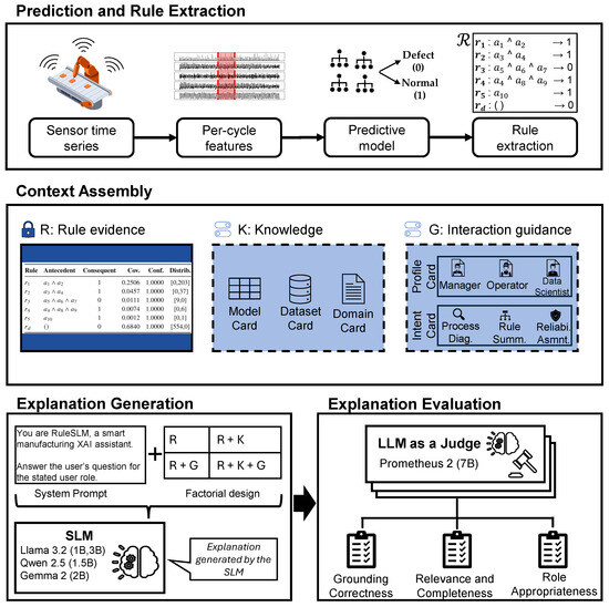
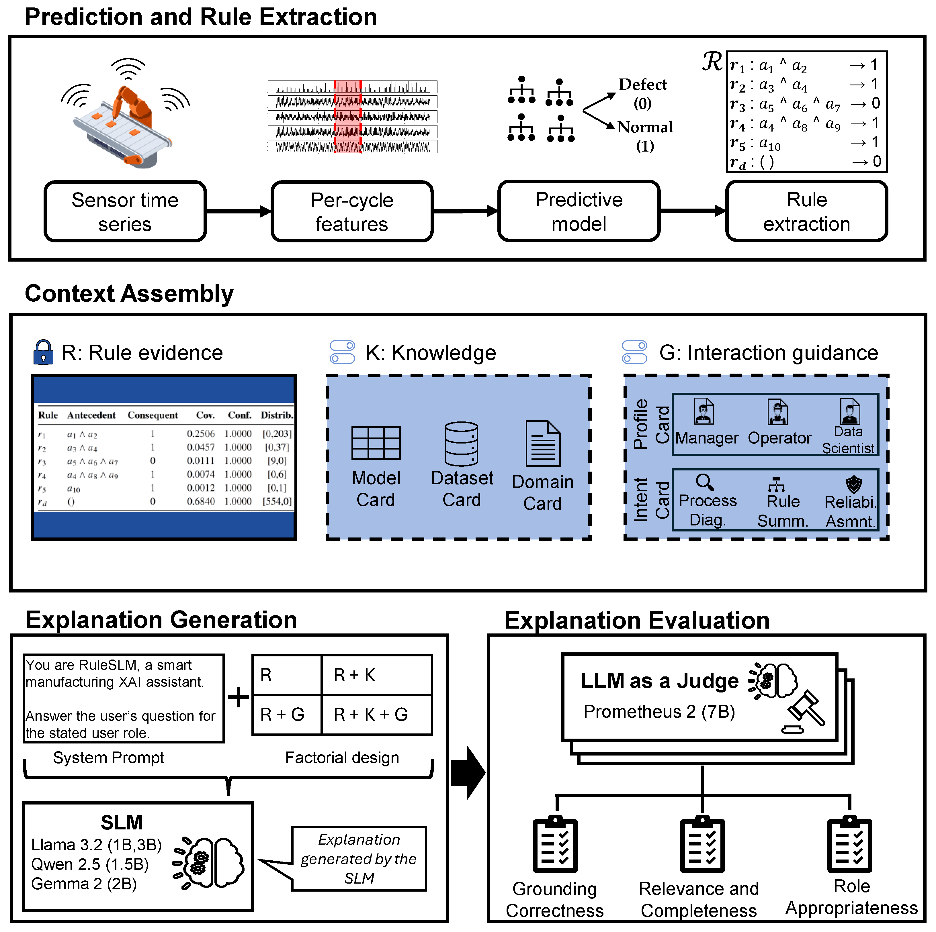
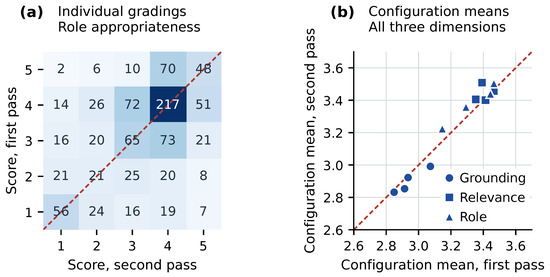
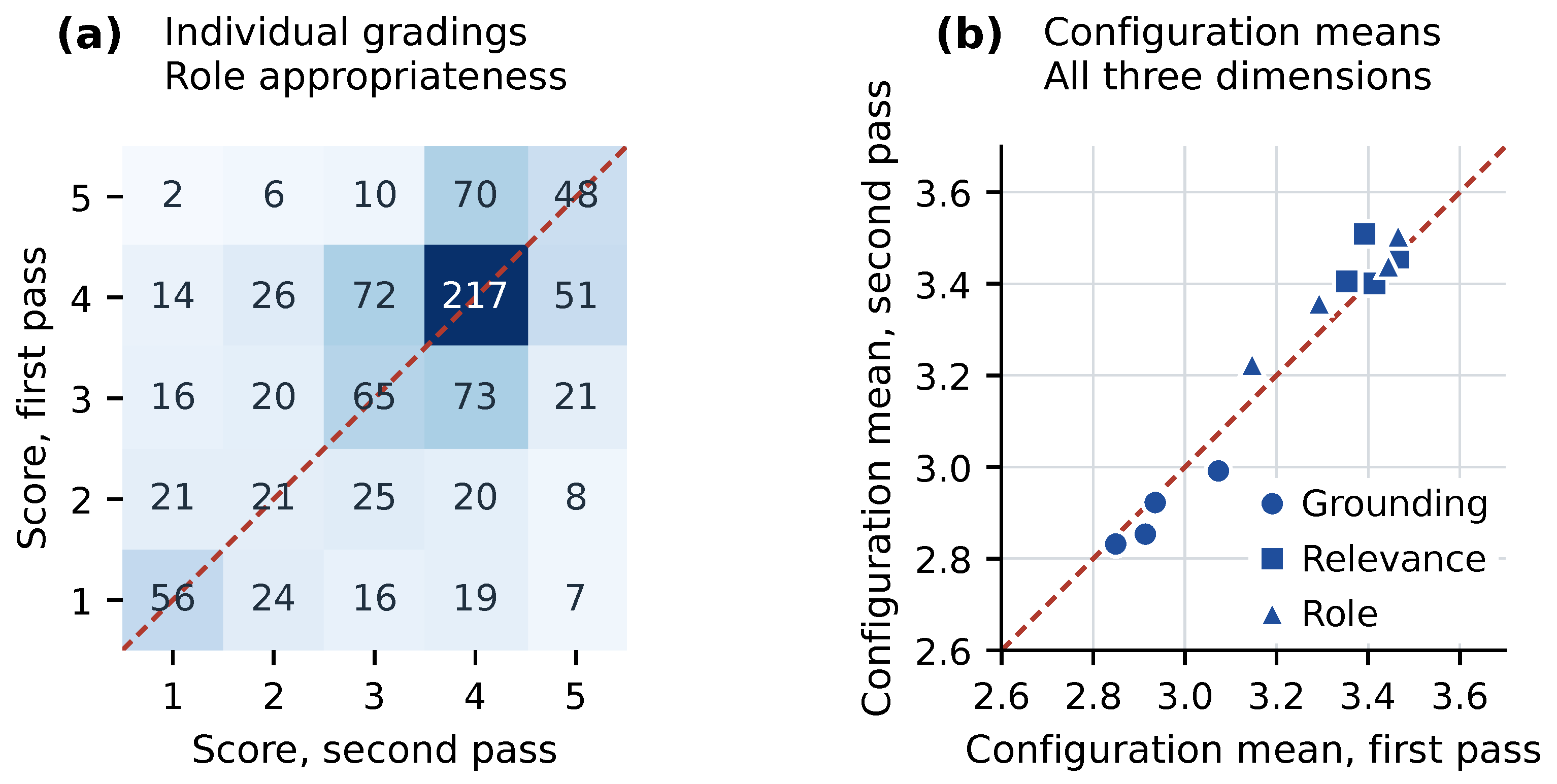
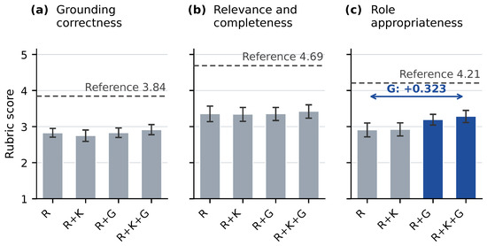
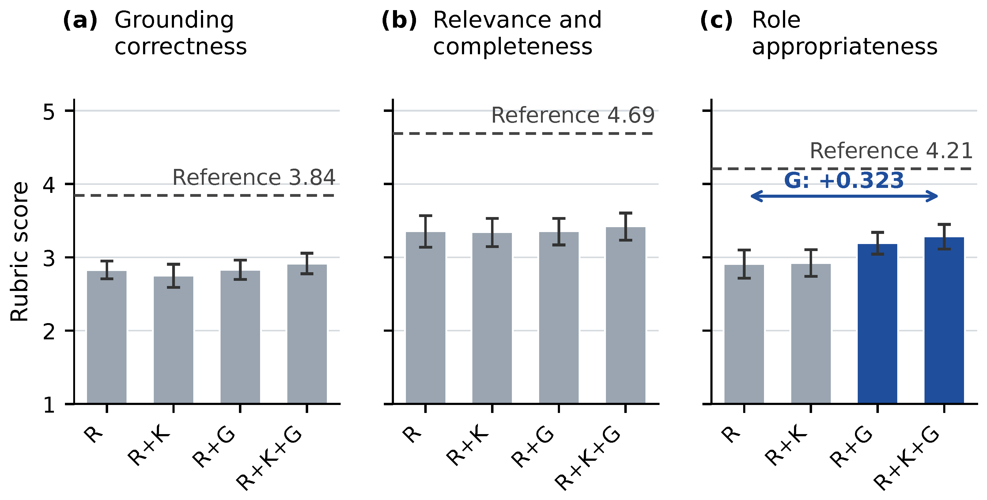
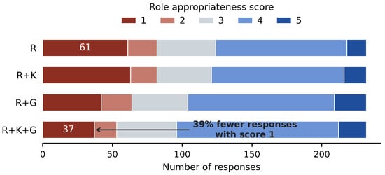
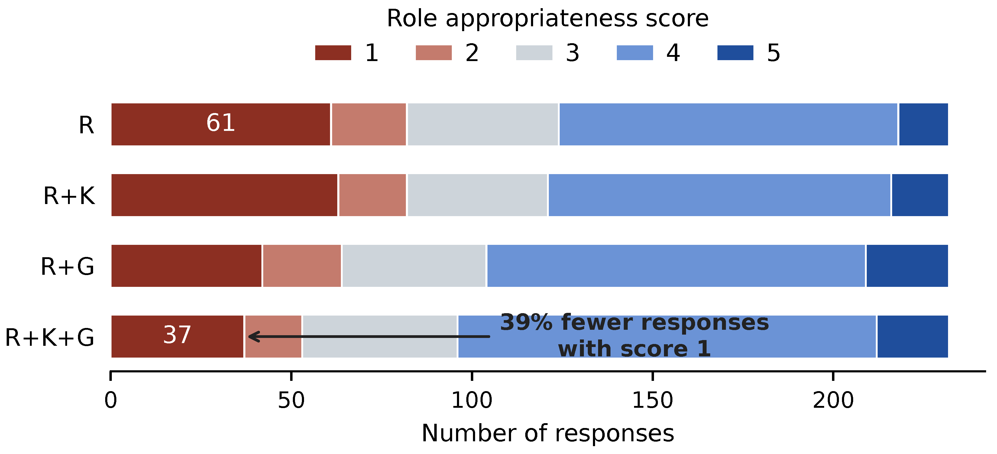
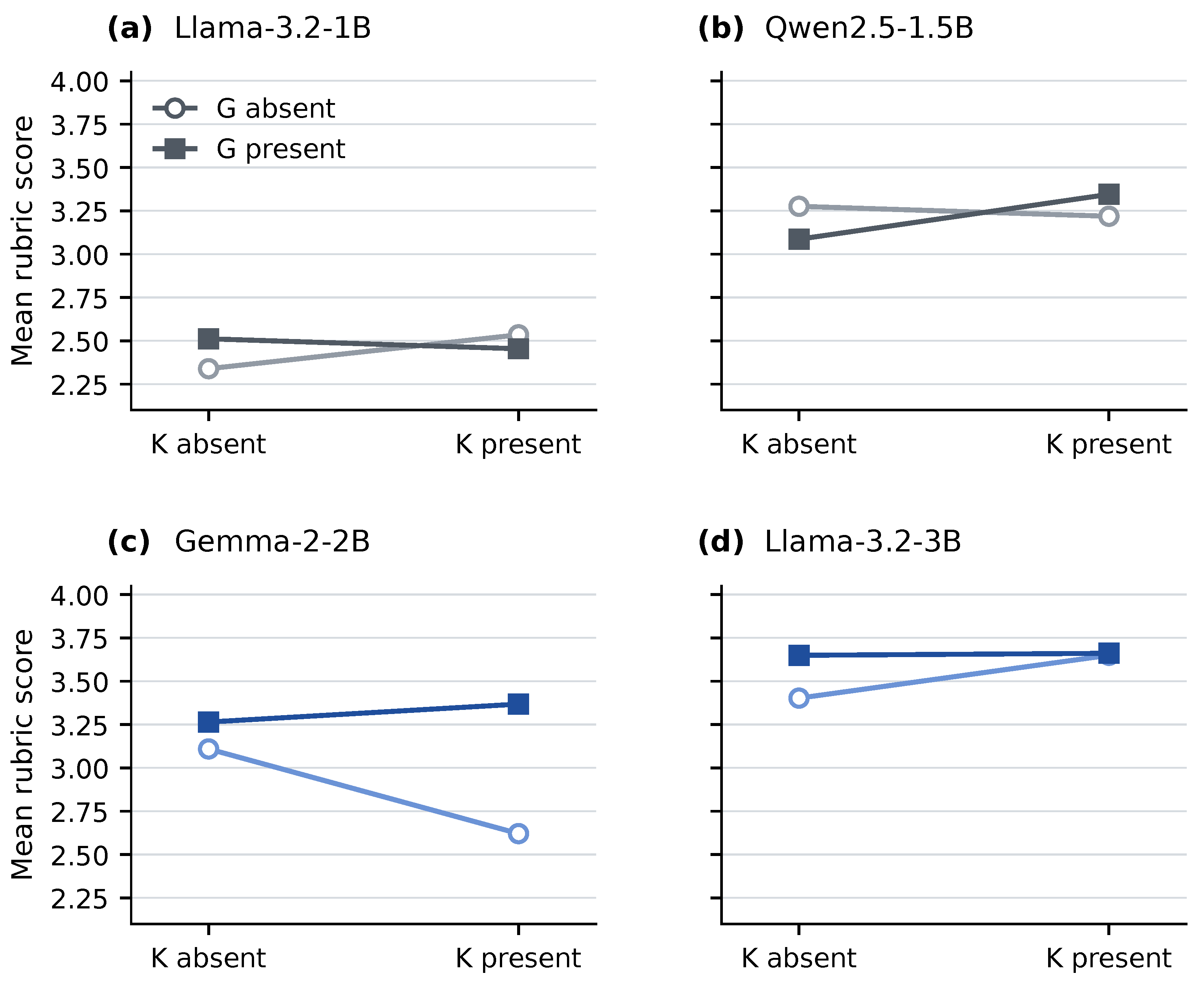
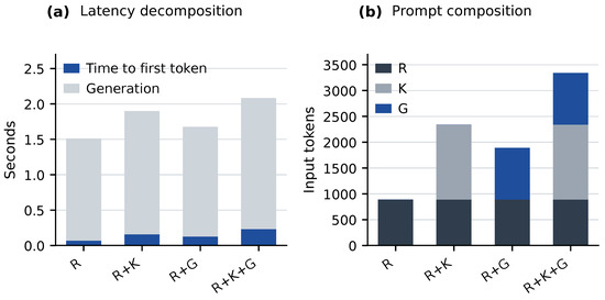
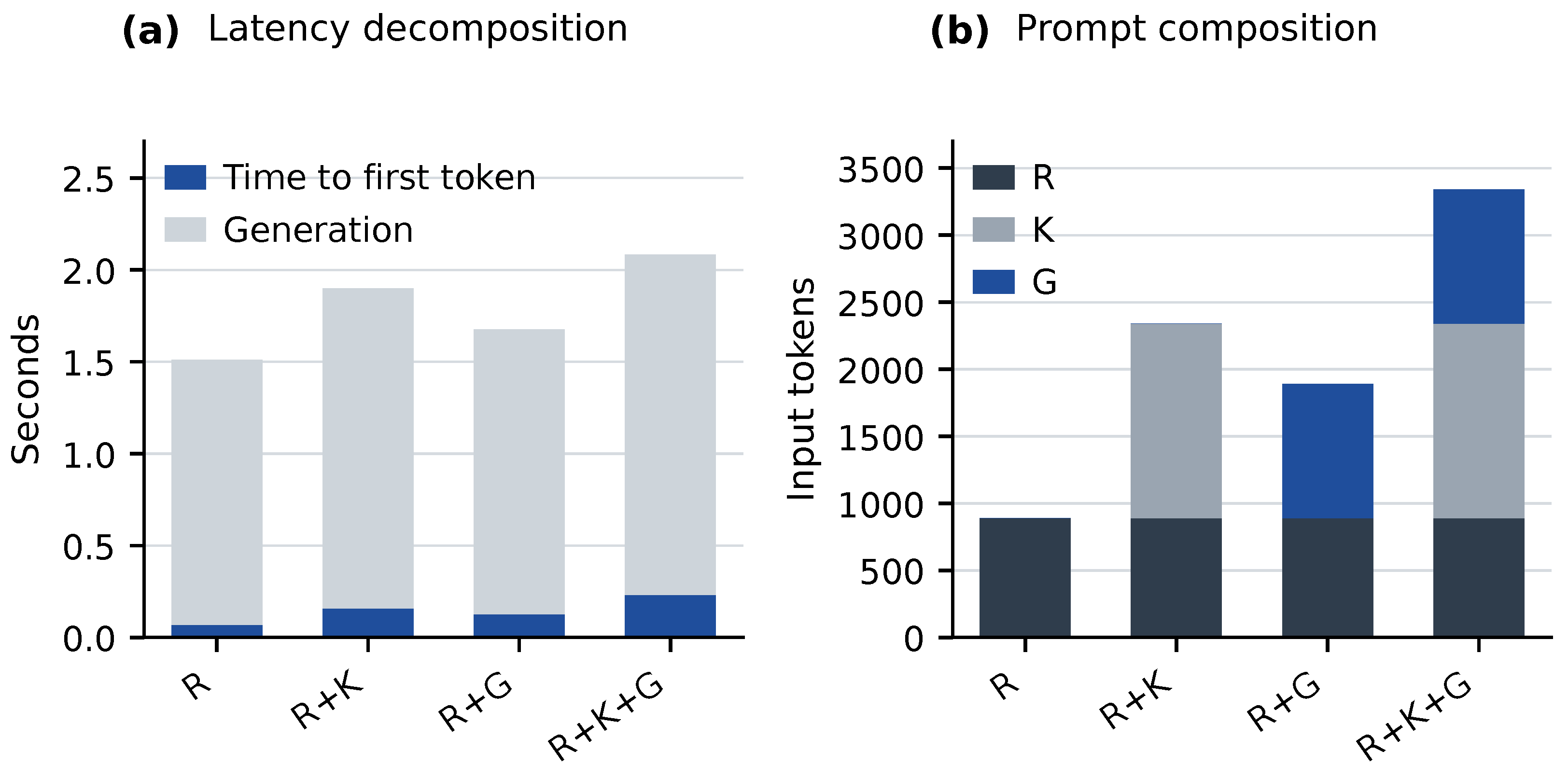
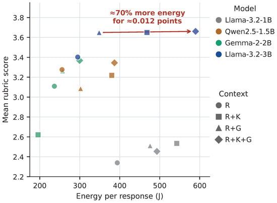
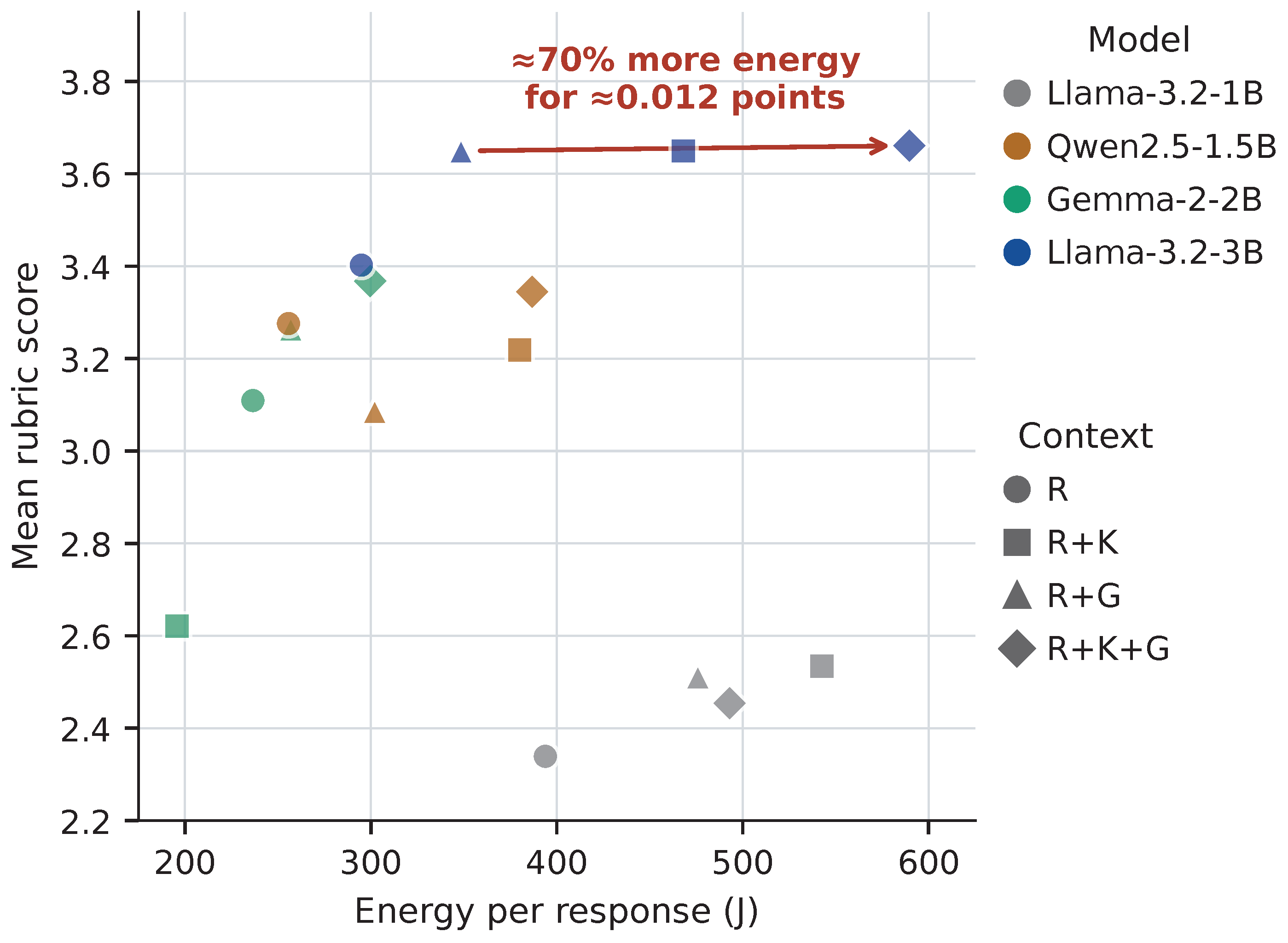

Disclaimer/Publisher’s Note: The statements, opinions and data contained in all publications are solely those of the individual author(s) and contributor(s) and not of MDPI and/or the editor(s). MDPI and/or the editor(s) disclaim responsibility for any injury to people or property resulting from any ideas, methods, instructions or products referred to in the content. |
© 2026 by the authors. Licensee MDPI, Basel, Switzerland. This article is an open access article distributed under the terms and conditions of the Creative Commons Attribution (CC BY) license.