Engineering Approximation of Saturated-Vapor P-v-T Behavior Using a Gas-Specific Temperature-Dependent Fitting Parameter: A Gas-Specific Empirical Correlation

Abstract

Accurate prediction of thermodynamic properties of real gases is essential for the analysis and design of energy systems such as power plants, gas turbines, and energy conversion processes. Although many equations of state have been developed, they still have limitations in accurately predicting the behavior of real gases, especially near the critical point. Unlike previous studies that focused on refining parameters embedded in conventional equations of state, this study introduces a gas-specific, data-driven approach by adjusting the specific gas constant in the ideal gas law. The gas-specific fitting parameter R_corr is evaluated directly from experimentally measured saturated-vapor P-v-T data and has the same units as the specific gas constant; however, it does not represent a modified or redefined physical gas constant. The proposed method should be interpreted as an empirical engineering correlation rather than as a predictive thermodynamic equation of state. Despite its simple formulation, the ideal gas law incorporating the corrected specific gas constant showed agreement with experimental data comparable to that of the Peng–Robinson–Stryjek–Vera equation of state over most of the saturation range, except near the critical point. For saturated steam, the proposed correlation reduced the pressure deviation to within approximately ±2.6% over most of the saturated-vapor region. Although the present assessment is limited to the dataset used to develop the correlation, the proposed correlation provides engineering-level accuracy while retaining a compact analytical form, making it suitable for repeated saturated-vapor P-v-T evaluations.

1. Introduction

Accurate evaluation of thermodynamic properties of gases and vapors is essential for the analysis and design of energy systems, including power plants, gas turbines, and energy conversion processes. Such properties are particularly important in the design and optimization of heat exchangers and thermal-fluid equipment, where real-gas deviations affect heat-transfer coefficients, pressure losses, and overall thermal efficiency. Thermophysical properties must often be evaluated repeatedly over wide temperature and pressure ranges; therefore, a simple yet accurate engineering-level model capable of representing real-gas behavior can offer substantial advantages over complex equations of state (EoS) [1,2].

Thermal-property evaluation is also fundamental to a wide range of energy systems. For example, the efficiency of various types of power plants is strongly affected by the thermal behavior of the working fluids, including steam and high-temperature gases supplied to turbines [3,4,5]. Likewise, in steam-reforming processes, where hydrocarbon fuels are converted into hydrogen, the thermal properties of steam play a decisive role in determining the reforming efficiency [6,7,8].

Recent IMO regulations have intensified interest in environmentally friendly alternative fuels for marine propulsion systems [9,10,11,12]. Methane (CH₄) and ammonia (NH₃) have been extensively investigated as alternative marine fuels [13,14,15,16,17,18], while methanol (CH₃OH) and hydrogen (H₂) have likewise attracted increasing attention [19,20,21,22,23,24]. Related thermodynamic studies have further demonstrated the importance of accurate thermophysical property evaluation in advanced energy systems, including natural gas/hydrogen-fueled compressed air energy storage systems [25] and integrated gas turbine-based energy systems with cascade heat recovery [26]. Since these fuels are commonly supplied to marine engines in gaseous form, reliable prediction of their thermophysical properties is crucial for evaluating combustion performance, heat-transfer characteristics, and overall thermal efficiency of internal combustion engines.

According to the State Postulate, a simple compressible system in thermodynamic equilibrium can be fully characterized by only two independent intensive properties. For gases or vapors, pressure (P), temperature (T), and volume (V) are typically selected as the primary independent variables. To determine any of these properties, a constitutive relationship among P-V-T must be specified. The simplest and most widely used equation is the ideal gas law, shown in Equation (1), which is often referred to as the ideal gas equation of state (ideal gas EoS).

$$Pv=RT$$

(1)

In Equation (1), the specific volume v is used instead of the total volume of V for simplicity since all thermal property data for gases and vapors are generally reported based on specific volume. The ideal gas law is based on idealized assumptions: gas molecules are considered point particles that move in straight lines due to the absence of intermolecular interactions. Therefore, applying Equation (1) to real gases results in large deviations from experimental data, particularly at high pressures and near the vapor–liquid equilibrium (VLE) region.

One of the earliest and most influential modifications of the ideal gas law is the van der Waals (vdW) equation [27,28,29,30], as shown in Equation (2).

$$P={\displaystyle \frac{RT}{\left(v-b\right)}}-{\displaystyle \frac{a}{v^2}} \mathrm{or} \left(P+{\displaystyle \frac{a}{v^2}}\right)\left(v-b\right)=RT,$$

(2)

$$a={\displaystyle \frac{9}{8}}R{T}_{cr}{v}_{cr},$$

$$b={\displaystyle \frac{1}{3}}{v}_{cr},$$

where a and b are the van der Waals constants, and the subscript cr denotes the critical state.

Other typical equations of state include the Redlich–Kwong (RK) EoS [31,32], Soave–Redlich-Kwong (SRK) EoS [33,34], Peng–Robinson (PR) EoS [35,36,37], and Peng–Robinson–Stryjek–Vera (PRSV) EoS [38,39,40]. Among them, the PRSV EoS, shown in Equation (3), has been widely recognized as providing accurate predictions of real-gas behavior over wide ranges of thermodynamic conditions.

$$P={\displaystyle \frac{RT}{\left(v-b\right)}}-{\displaystyle \frac{a}{v^2+2bv-b^2}},$$

(3)

where $a={\displaystyle \frac{0.457235R^2{T}_{cr}^2}{P_{cr}}}\times \alpha \left(T\right)$ with the unit of N∙m⁴/kg², $b={\displaystyle \frac{0.077796R{T}_{cr}}{P_{cr}}}$ with the unit of m³/kg, and R is the specific gas constant.

The temperature-dependent coefficient α(T), included in a, is dimensionless and expressed as follows, where T denotes the absolute temperature in K:

$$\begin{gathered} \alpha \left(T\right)={\left[1+k\left(1-\sqrt{T_r}\right)\right]}^2,\mathrm{where} \\ {T}_r={\displaystyle \frac{T}{T_{cr}}}, \\ k=k_0+k_1\left(1+\sqrt{T_r}\right)\times \left(0.7-T_r\right), \\ {k}_0=0.378893+1.4897153w-0.17121848w^2+0.0196554w^3,\mathrm{and} \\ w=-{\log }_{10}\left({\displaystyle \frac{P_{sat @ T_r=0.7}}{P_{cr}}}\right)-1. \end{gathered}$$

However, the PRSV EoS has the drawback of including relatively complex parameters, which can limit its convenience for rapid or repetitive engineering calculations. In contrast, recent studies by Choi et al. employed the ideal gas law to calculate the thermodynamic properties of steam in a simplified framework [30,41]. Their method showed good agreement with experimental data over the superheated-steam region covered by the ASME Steam Tables [38], demonstrating that the ideal gas framework can be extended to approximate real-gas behavior over a wide range of thermodynamic conditions.

To improve the agreement between the ideal gas law and experimentally measured properties while retaining its simple form, a data-driven correction strategy based on the ideal gas law is adopted in this study. A temperature-dependent fitting parameter with the same units as the specific gas constant is introduced into the ideal-gas-form equation using experimentally measured saturated-vapor P-v-T data. This study does not aim to develop a universal or predictive equation of state applicable to all gases. Instead, it proposes a gas-specific empirical engineering correlation that preserves the simplicity of the ideal gas law while reducing deviations in saturated-vapor P-v-T evaluation. This approach addresses the need for a simple and rapidly evaluable correction framework for engineering calculations in which repeated property evaluation is required within a limited thermodynamic path. The main contribution of this study is therefore the development and assessment of a simple correction framework for rapid and repeated saturated-vapor P-v-T evaluations within the fitted saturated-vapor range.

2. Comparison of the Saturation Pressure (P_sat) with the Saturation Temperature (T_sat) Based on the Ideal Gas Law and Experimental Data

The prediction of the thermophysical properties of gases or vapors relies on empirical equations based on experimental data, theoretical equations derived purely from fundamental principles, or semi-empirical equations that incorporate experimental data into theoretical formulations. The ideal gas law, which is derived from an idealized theoretical model, can be regarded as a simplified theoretical equation. In contrast, the vdW EoS can be regarded as a semi-empirical equation in which the concept of intermolecular attraction is incorporated into the ideal gas law.

Although the ideal gas law was developed for an ideal gas and the vdW EoS was developed for real gases, both equations commonly exhibit significant deviations when their calculated predictions are compared with experimental data. These deviations become particularly pronounced at high pressures and near the VLE region, where real-gas effects such as intermolecular attraction and finite molecular volume become significant. While the vdW EoS shows better agreement with experimental data than the ideal gas law, its accuracy is still limited. Therefore, numerous EoSs, as mentioned in the previous section, have been introduced to reduce these discrepancies, and most of them are essentially modified versions of the vdW EoS with progressively increasing mathematical complexity.

As seen in Equations (1)–(3), EoSs have evolved from simple to increasingly complex forms in order to improve predictive accuracy. However, while simpler equations are easier to compute, they tend to produce larger deviations from experimental data. In contrast, more complex equations are computationally cumbersome but yield results that are closer to experimental data over a broader range of thermodynamic conditions.

Figure 1 compares the variation of P_sat-T_sat relationship for steam obtained from experimentally tabulated data and the results calculated using three EoSs: the ideal gas law, the vdW EoS and the PRSV EoS. The PRSV EoS results presented in Figure 1 were calculated following standard formulations reported in the literature and are included here as a benchmark for comparison with simpler correlations.

To construct Figure 1, the values of the coefficients included in Equations (1)–(3) must first be determined using the thermodynamic properties of steam. Since the critical properties of steam are P_cr = 22.064 MPa, v_cr = 0.003106 m³/kg, T_cr = 647.096 K, and the specific gas constant R is 461.521 J/kg∙K, the vdW coefficients in Equation (2) are constants calculated as a = 1045.1173 N∙m⁴/kg² and b = 1.03533 × 10⁻³ m³/kg [30]. In contrast, the coefficient b in the PRSV EoS of Equation (3) is also a constant and its value is b = 1.05274 × 10⁻³ m³/kg, while the coefficient a is a temperature-dependent variable introduced to improve agreement with experimental data.

To calculate the coefficient a in the PRSV EoS, the acentric factor, commonly denoted as w, must be specified. The acentric factor was first introduced and evaluated by Pitzer, who reported a value of w = 0.344 for steam in 1955 [42]. Since then, its value proposed by Pitzer has been continuously refined to minimize the deviations between the calculated P-v-T data and experimental measurements. In 1986, Stryjek and Vera [38] proposed w = 0.34380 and k₁ = −0.06635 for steam without refitting to the present dataset, and these values are used in the calculation of the coefficient a for constructing Figure 1 as a representative high-accuracy reference model.

Figure 1. Comparison of the P_sat-T_sat relationship for steam obtained from experimental data and the three EoSs: the ideal gas law, the vdw EoS and the PRSV EoS. It should be noted that different y-axis scales are used in the three panels to improve the visibility of the individual comparisons. The experimental dataset of (T_sat, P_sat) consists of 165 points in total. The PRSV EoS shows a deviation of approximately −5% at the last two points near the critical region. The experimental data were taken from the ASME Steam Tables [43]. (a) Experimental data vs. the results calculated using the ideal gas law. (b) Experimental data vs. the results calculated using the vdW EoS. (c) Experimental data vs. the results calculated using the PRSV EoS.

Figure 1. Comparison of the P_sat-T_sat relationship for steam obtained from experimental data and the three EoSs: the ideal gas law, the vdw EoS and the PRSV EoS. It should be noted that different y-axis scales are used in the three panels to improve the visibility of the individual comparisons. The experimental dataset of (T_sat, P_sat) consists of 165 points in total. The PRSV EoS shows a deviation of approximately −5% at the last two points near the critical region. The experimental data were taken from the ASME Steam Tables [43]. (a) Experimental data vs. the results calculated using the ideal gas law. (b) Experimental data vs. the results calculated using the vdW EoS. (c) Experimental data vs. the results calculated using the PRSV EoS.

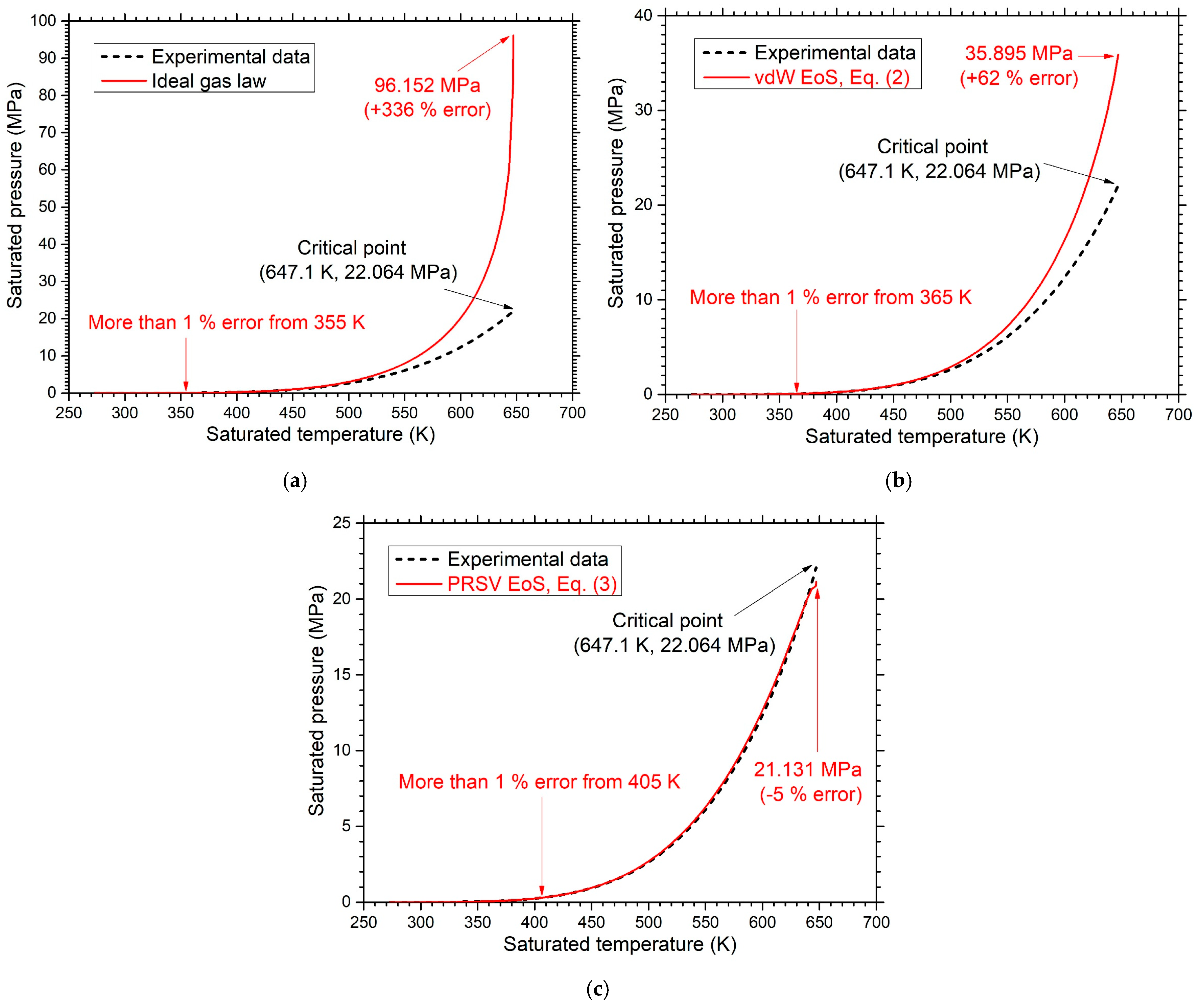
The experimental data shown in Figure 1 consist of a total of 165 data points, which were compiled by combining the temperature-based and pressure-based properties provided in the ASME Steam Tables. As shown in Figure 1, the prediction of P_sat by the PRSV EoS is the closest to the experimental data, except for the last two points (646.86 K and 647.10 K) near the critical point. The errors in all calculations remain within the range of −0.05 to +2.8% over the entire T_sat range. Although such errors may not be acceptable for precise scientific purposes, they are considered sufficiently accurate for engineering applications.

However, it should be noted that, even when evaluating P_sat as a function of temperature, the PRSV EoS involves solving a cubic equation with respect to the specific volume that includes several temperature-dependent parameters. This leads to multiple mathematical roots and requires additional considerations to identify the physically relevant solution, thereby substantially reducing its practical convenience for rapid or repeated engineering calculations, despite its high accuracy.

For this reason, while the PRSV EoS provides high predictive accuracy, its computational complexity can limit its practical usefulness in engineering calculations where simplicity and rapid evaluation are often required. It should also be noted that the purpose of this comparison shown in Figure 1 is not to establish a universally applicable or superior equation of state, but rather to provide a benchmark that motivates a simplified gas-specific engineering correction framework, in which real-gas deviations along the saturation line are represented by a temperature-dependent fitting parameter within the ideal-gas form.

3. Temperature-Dependent Fitting Parameter in the Ideal-Gas Form

The ideal gas law is simple but produces large errors when calculating the P-v-T behavior of real gases because it does not account for intermolecular interactions and the finite molecular volume. This indicates that the ideal gas law cannot serve as an accurate predictive model for describing the behavior of real gases, which has led to the development of numerous EoSs.

The development of an EoS beyond the ideal gas law can be said to have begun with the vdW EoS, which was later modified by Redlich and Kwong. Since then, many efforts to develop new EoSs have primarily focused on refining the coefficients of existing models to improve their accuracy. However, the authors questioned whether such highly complex forms of EoSs are always necessary for engineering-level evaluations of real-gas behavior. By examining the discrepancies between the ideal gas law and the experimental data shown in Figure 1a, they hypothesized that real-gas effects could be incorporated into the ideal gas law through a gas-specific correction framework, rather than by proposing a new universal EoS.

3.1. Corrected Specific Gas Constant Derived from Parameter Estimation of the Deviation Data

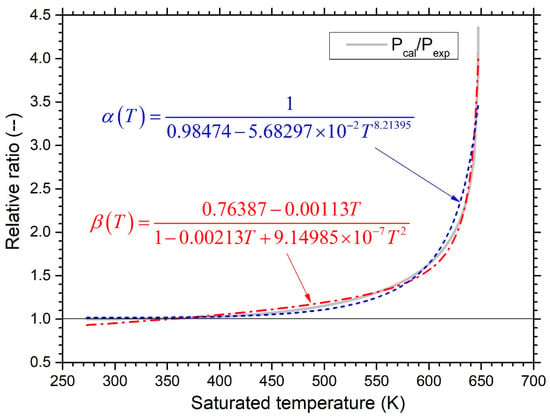
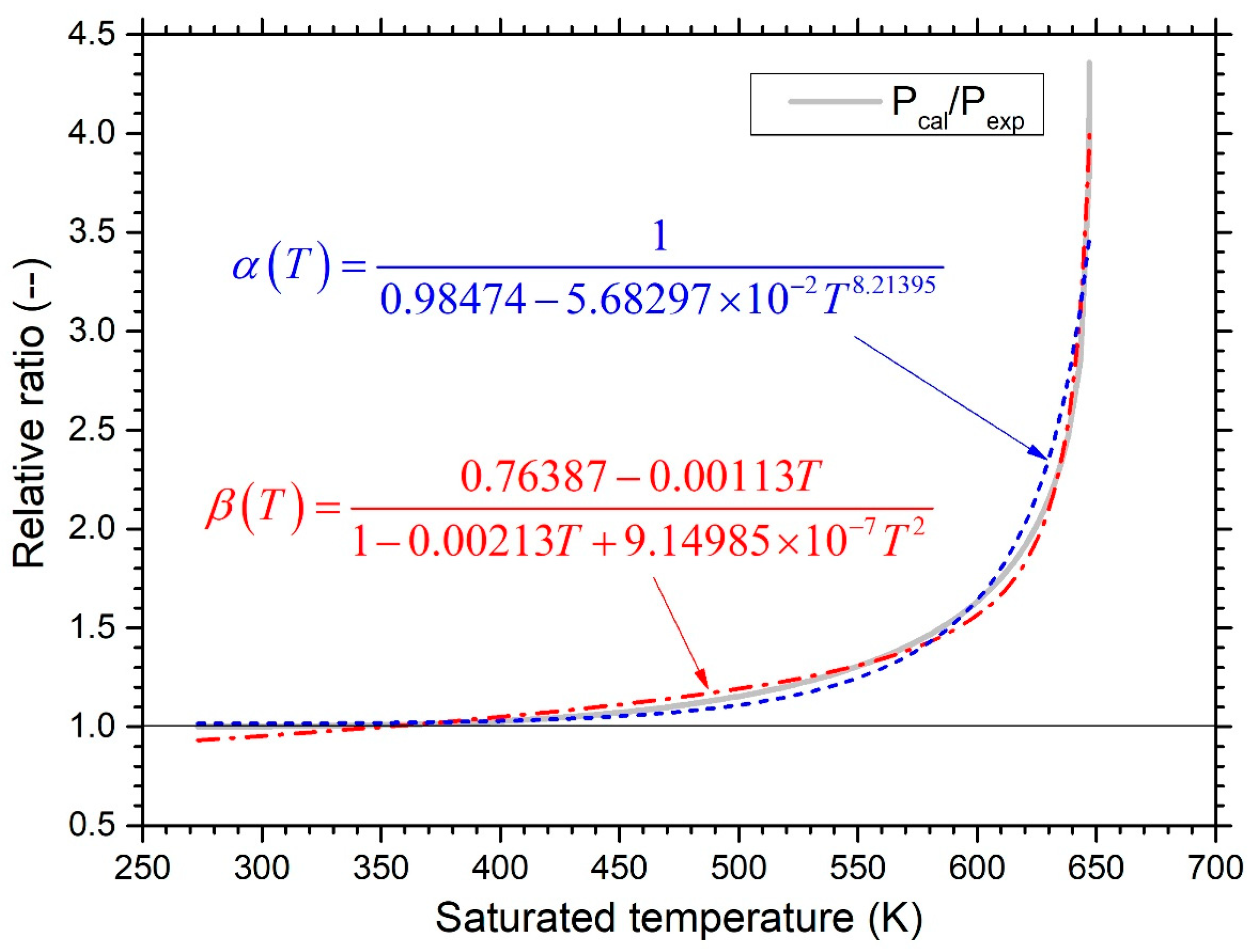
Figure 1a illustrates the deviation between P_sat predicted by the ideal gas law and the corresponding experimental data provided in the ASME Steam Tables, where the deviation appears to increase monotonically and exhibits a rapid nonlinear increase with temperature. To analyze this deviation more clearly, the relative ratio defined as P_cal/P_exp is introduced.

In Figure 2, the gray solid line represents the ratio of the calculated values to the experimental data, while the dashed lines indicate two fitted curves corresponding to this ratio. Candidate functional forms were first screened based on their ability to represent the observed trend. Their performance was then assessed quantitatively using the RMSE and maximum absolute relative pressure deviation obtained after substitution into the ideal-gas-form equation. These quantitative criteria, rather than visual agreement alone, were used to assess the retained functional forms.

Figure 2. The ratio defined as P_cal/P_exp, where P_cal is P_sat calculated using the ideal gas law and P_exp is the experimental P_sat of steam, which was taken from the ASME Steam Table [43]. The gray solid line represents the calculated ratio, while the dashed curves represent fitted functions obtained using a rational function and power function.

Based on the trends observed in Figure 2, the rational function β is expected to produce slightly larger errors than the power function α in the low-temperature region and near the critical point. However, when the two approximated functions are compared over the entire temperature range, the overall deviation associated with β remains smaller than that of α, and the rational function β is found to maintain deviations within an acceptable margin for engineering applications, whereas the power function α exhibits larger localized deviations. Since the temperature-dependent coefficient β shown in Figure 2 represents the deviation of the ideal-gas prediction from the experimental data, the ideal-gas pressure can be adjusted to better match the experimental data as follows.

$$P=R_{corr}{\displaystyle \frac{T}{v}}={\displaystyle \frac{R}{\beta \left(T\right)}}{\displaystyle \frac{T}{v}},$$

(4)

$$\mathrm{where} R_{corr}={\displaystyle \frac{R}{\beta \left(T\right)}},\mathrm{and}$$

(5)

$$\beta \left(T\right)={\displaystyle \frac{0.76387-0.00113T}{1-0.00213T+9.14985\times {10}^{-7}{T}^2}}.$$

(6)

In Equation (4), R/β corresponds to the corrected specific gas constant of steam, denoted as R_corr. Since the pressure calculated by the ideal gas law is consistently greater than the experimental data, as shown in Figure 1a, the coefficient β must appear in the denominator of the last term in Equation (4).

The comparison between the PRSV EoS and the modified ideal gas law of Equation (4), which employs the corrected specific gas constant, will clearly highlight the extent to which this study aims to retain a compact analytical form while accounting for real-gas effects. The validity of Equation (4) will be discussed in the following section through comparison with the experimental data.

3.2. Corrected Specific Gas Constant R_corr and Its Approximation

As already mentioned, the ideal gas law is by no means an appropriate model for describing the behavior of real gases. However, compared with other EoSs developed after the vdW EoS, its simplicity remains an undeniable advantage. Section 3.1 presented the first attempt to introduce a correction factor to align the pressure calculated by the ideal gas law with the experimentally measured pressure. It should be emphasized that the discussion in this section does not aim to reinterpret or reformulate the ideal gas law as a universal EoS for real gases. Rather, the objective is to introduce a gas-specific correction framework that preserves the simplicity of the ideal gas law while reducing the deviation between the ideal-gas prediction and the experimental saturated P-v-T data through a temperature-dependent fitting parameter.

In this subsection, a correction factor based on a conceptually different approach is introduced. Nevertheless, since only a single coefficient is used, it ultimately takes the same form as Equation (4). Considering that the P-v-T properties in the ideal gas law of Equation (1) are directly measurable, the only parameter that can be adjusted to match the calculated pressure with the experimental data is the specific gas constant R. Although a correction factor to adjust the value of R is introduced in this study, it should be noted that R is inherently defined as a unique constant. If the ideal gas law is rearranged to solve for R,

$$R_{corr}={\displaystyle \frac{P_{exp}{v}_{exp}}{T_{exp}}},$$

(7)

here, P_exp-v_exp-T_exp are experimentally measured properties. That is, these quantities correspond to the property values tabulated in standard reference data sources, such as the ASME Steam Tables.

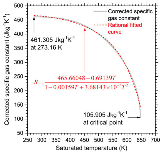
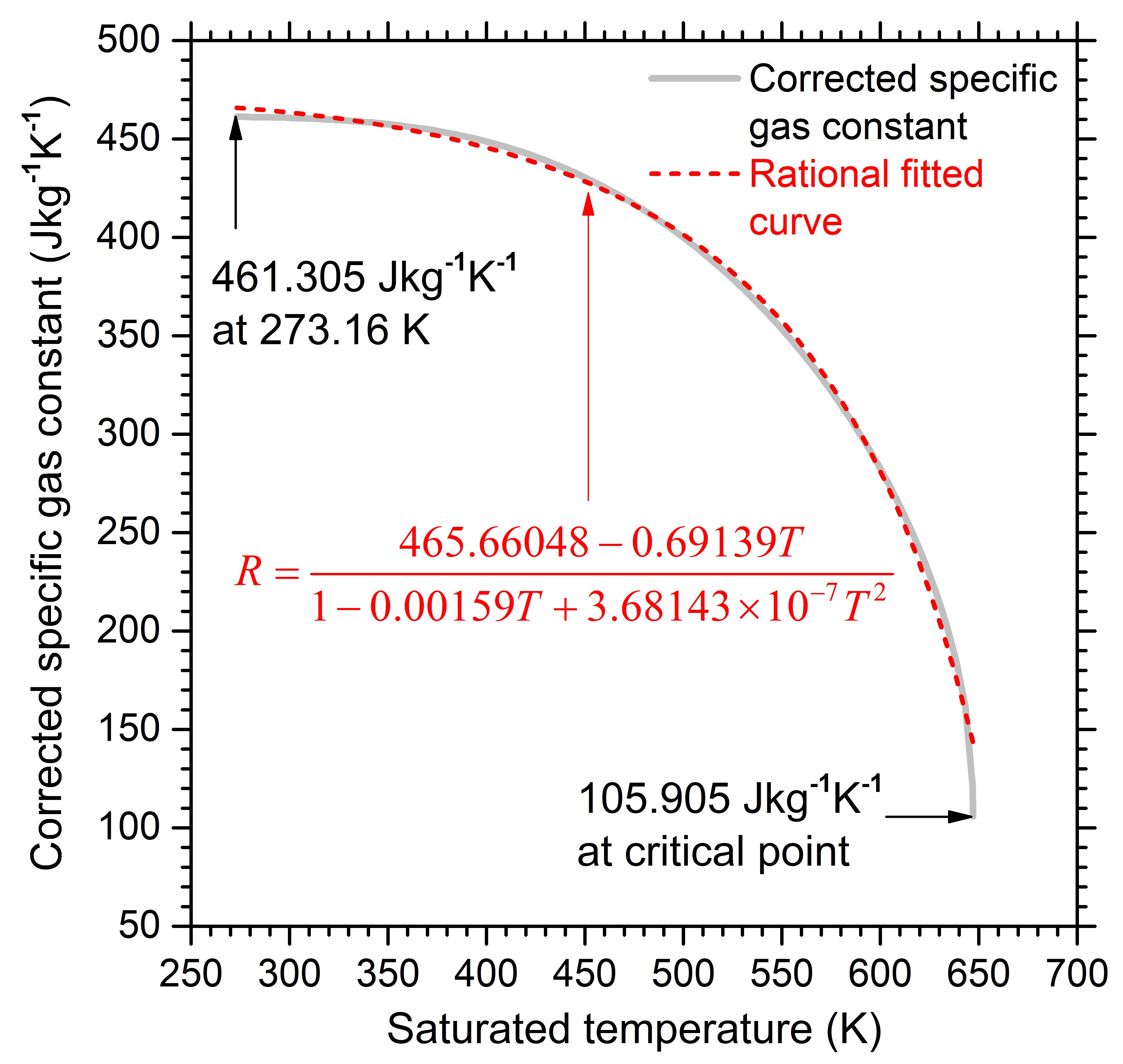
If the pressure is evaluated using the ideal gas law based on the measured temperature T and specific volume v, the calculated pressure inevitably deviates from the measured pressure due to the inherent limitations of the ideal gas model. Therefore, when the measured P-v-T values are substituted into Equation (7), the resulting value, referred to hereinafter as R_corr, differs from R = 461.521 J/kg∙K. Figure 3 shows the variation of the corrected specific gas constant R_corr evaluated from the measured P-v-T values over the entire range of saturated temperatures of steam. In this study, R_corr should not be interpreted as a new gas constant, a virial coefficient, or a dimensionless compressibility factor. Rather, it is a temperature-dependent fitting parameter with the same units as R, which is introduced to reduce the deviation of the ideal gas law for the saturated-vapor P-v-T data considered in this study.

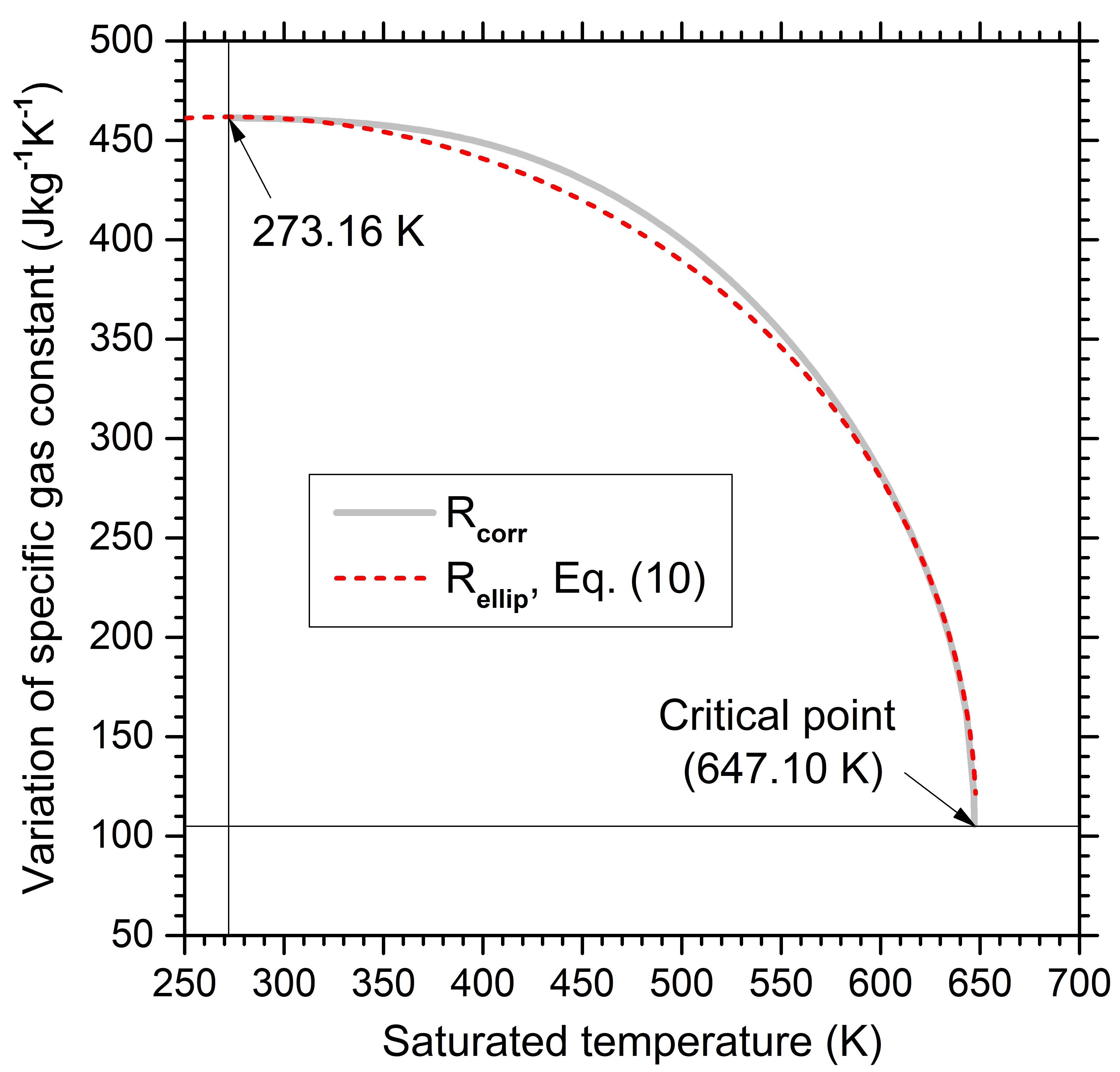
Figure 3. Variation of the corrected specific gas constant R_corr evaluated using Equation (7), where the P-v-T values are taken from the ASME Steam Tables [43]. The gray solid line represents R_corr, and the red dashed line represents the rational fitted curve. Unlike the previous figures, to emphasize the elliptical shape of the curve, the 1:1 aspect ratio was intentionally applied to this graph by setting both axis ranges to the same numerical value of 450 with identical tick spacing.

In Figure 3, the gray solid line shows the variation of the corrected specific gas constant R_corr calculated using Equation (7) based on the measured P-v-T values, and the dashed line represents the approximated curve expressed as a rational function. If the corrected specific gas constant R_corr is used to calculate the pressure,

$$P=\gamma \left(T\right){\displaystyle \frac{T}{v}},\mathrm{where}$$

(8)

$$\gamma \left(T\right)={\displaystyle \frac{465.66048-0.69139T}{1-0.00159T+3.68143\times {10}^{-7}{T}^2}}.$$

(9)

The corrected specific gas constant, denoted as γ(T) must have the same units as the specific gas constant R and is treated as a temperature-dependent variable. As can be seen in Figure 3, near the critical point (i.e., the last two data points), the approximated curve γ representing R_corr exhibits a non-negligible difference.

This leads to the results similar to those obtained using the PRSV EoS at the critical point, as shown in Figure 1c. As noted in the caption of Figure 3, the 1:1 aspect-ratio plot suggests that the variation of the corrected specific gas constant R_corr can be approximated by an elliptical function. This ellipse is introduced solely as an empirical geometric fitting form and is not intended to imply a physical mechanism or thermodynamic basis.

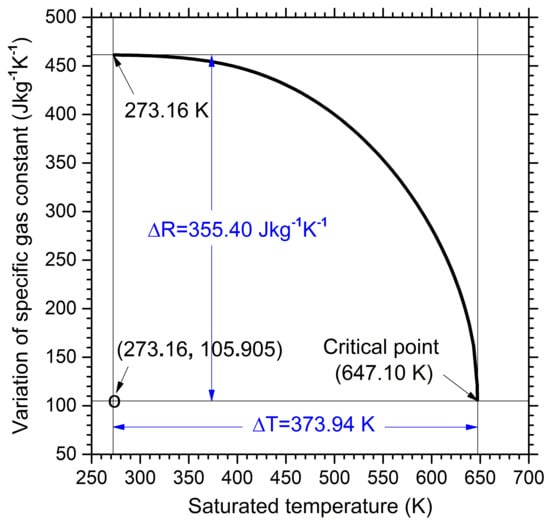
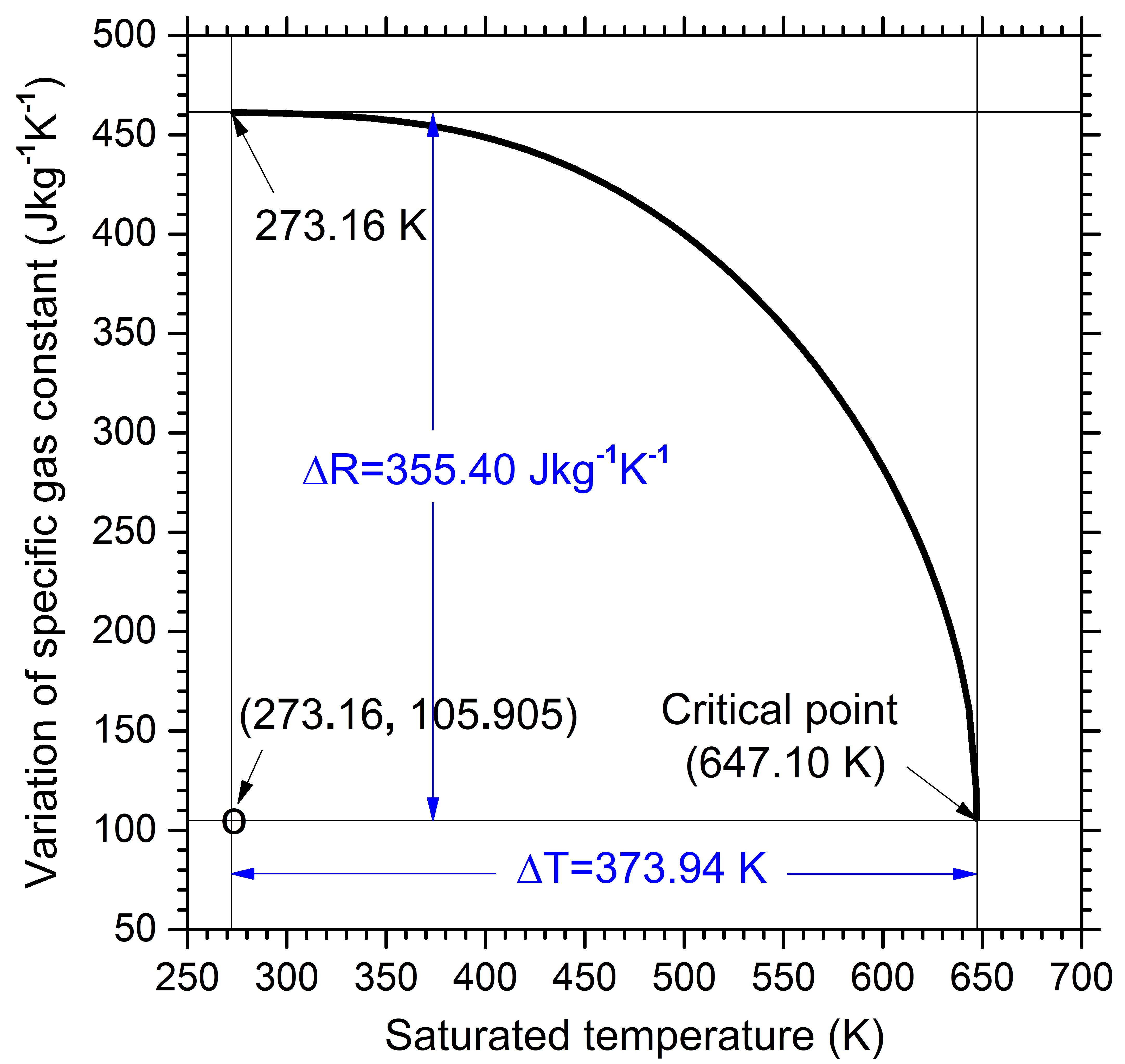
Figure 4 presents the numerical values of the major and minor axes used to approximate R_corr with an elliptical equation. When the corrected specific gas constant R_corr is approximated by an elliptical equation, the major axis corresponds to the temperature axis, and the minor axis corresponds to the axis of the corrected specific gas constant R_corr. Since the approximated elliptical equation deviates from R_corr, it is denoted as R_ellips. Then, the standard form of the ellipse is given by

$${\displaystyle \frac{T^2}{{373.94}^2}}+{\displaystyle \frac{R_{ellip}^2}{{355.40}^2}}=1.$$

Figure 4. Values of the major and minor axes used to approximate the corrected specific gas constant R_corr with an elliptical equation. The center of the ellipse is located at (273.160, 105.905). As in Figure 3, this graph was plotted with a 1:1 aspect ratio to emphasize the elliptical shape.

However, considering that the center of the ellipse is located at (273.160, 105.905), as shown in Figure 4, the equation of the ellipse is given by

$${\displaystyle \frac{{\left(T-273.160\right)}^2}{{373.94}^2}}+{\displaystyle \frac{{\left(R_{ellip}-105.905\right)}^2}{{355.40}^2}}=1.$$

(10)

Rearranging Equation (10) for R_ellip,

$$R_{ellip}=105.905+355.905\sqrt{ \left[1-{\displaystyle \frac{{\left(T-273.16\right)}^2}{{\left(373.94\right)}^2}}\right] }.$$

(11)

Since the pressure of steam is calculated using the ideal gas law, Equation (11) serves to correct the specific gas constant R and is denoted as the correction factor δ(T) hereafter. Then the pressure is calculated as

$$P=\delta \left(T\right){\displaystyle \frac{T}{v}},$$

(12)

where δ(T) is Equation (11), i.e., δ(T) = R_ellip, and has the same units as R.

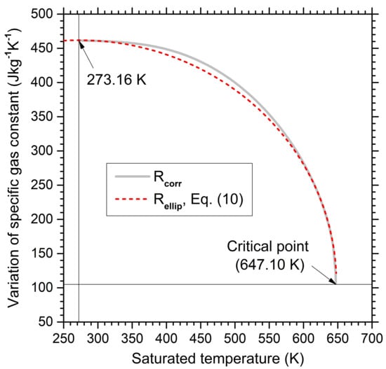
Figure 5 shows the elliptical curve plotted using Equation (11). It should be noted that the elliptical approximation represents one possible geometric representation of R_corr for steam and should not be interpreted as a universal correction function applicable to all gases.

Figure 5. Elliptical approximation of the corrected specific gas constant R_corr. The excellent agreement of R_ellip with R_corr is observed in both the low temperature region and the high temperature region.

Compared with Figure 3 and Figure 5, the correction factor δ shown in Figure 5 generally exhibits good agreement with R_corr in both the low- and high-temperature regions. However, a non-negligible deviation is still expected near the critical point, and the agreement in the intermediate saturated temperature region is also found to be somewhat unsatisfactory. The agreement between all correction factors and the experimental data will be examined in the following section.

4. Accuracy Assessment of the Corrected Specific Gas Constant R_corr

In this section, the accuracy of the three correction factors (β, γ, and δ) mentioned in the previous section is systematically assessed using two different methods. First, to evaluate how accurately the correction factors reproduce the experimental data, the deviation between P_sat calculated using the corrected ideal gas law and the experimental data is examined. In this comparison, P_sat calculated using the PRSV EoS is also included solely as a reference model, since it is widely regarded as one of the most accurate EoSs currently available. This comparison is intended to assess the relative performance of the proposed gas-specific correction framework, rather than to establish it as a universally applicable or superior equation of state.

The dataset roles are explicitly distinguished in this study. The 165 saturated-vapor data points from the ASME Steam Tables constitute the development dataset used to derive the fitting parameters. The comparison against these same ASME data is therefore treated as an in-sample reproduction assessment and not as independent validation. This choice is appropriate because the present study aims to assess the applicability of the proposed ideal-gas-form correction for saturated-vapor P-v-T evaluation, rather than for general superheated-vapor, supercritical, or saturated-liquid states. The saturated-temperature range considered in this study covers the full range from 273.16 K to 647.10 K for steam, including the low-temperature, intermediate-temperature, high-temperature, and near-critical regions. Therefore, the selected verification conditions are representative for evaluating both the applicability and the limitations of the proposed correlation within the fitted saturated-vapor range.

Secondly, the calculated P_sat is substituted back into Equation (12), rearranged for the specific volume. Because the same equation and correction function are used in both calculations, this procedure is algebraically dependent and should not be interpreted as an independent validation. The comparison is included only to illustrate the internal consistency of the calculation and to provide a reference comparison with the PRSV EoS.

4.1. Comparison of the Saturated Pressures

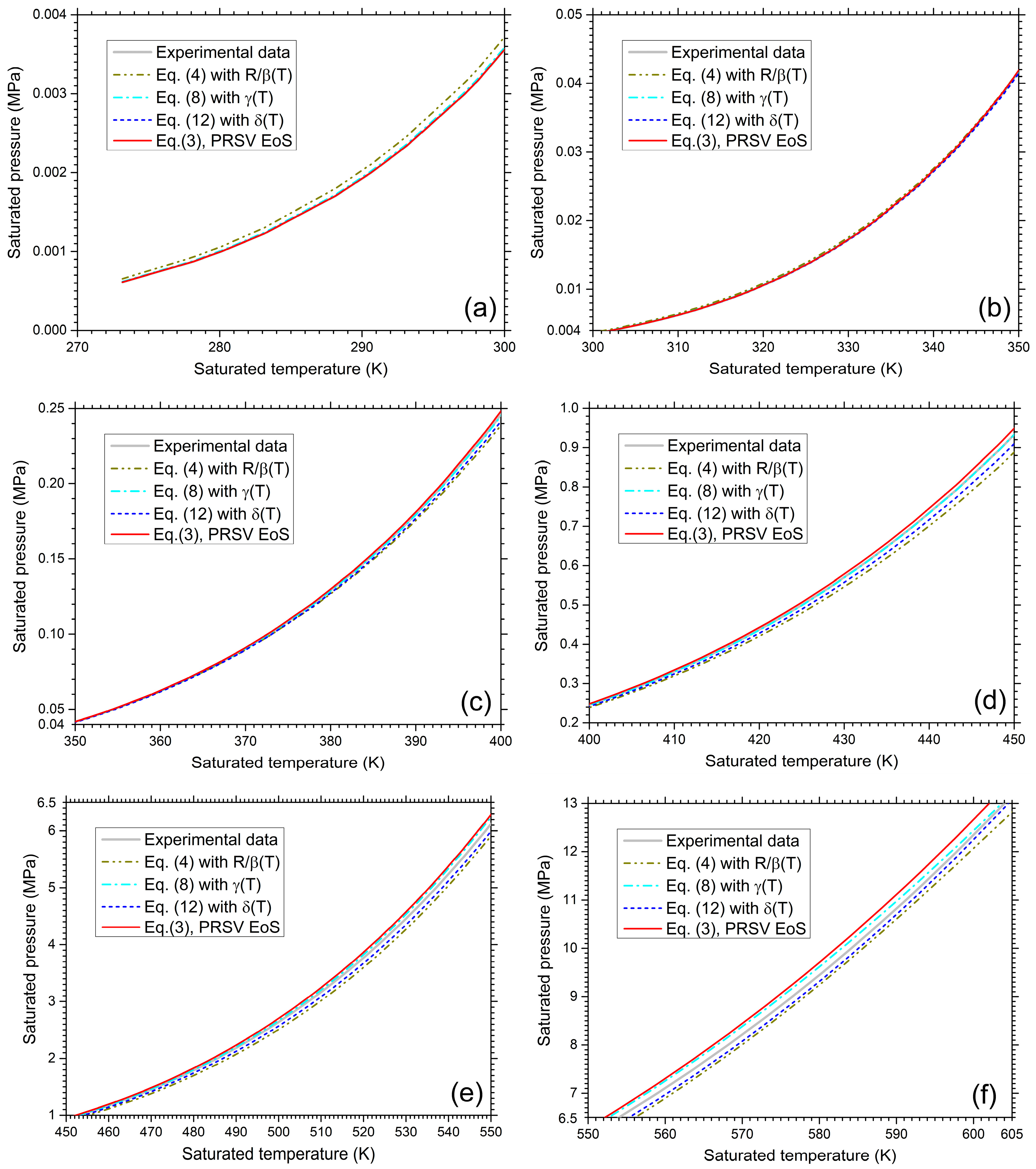
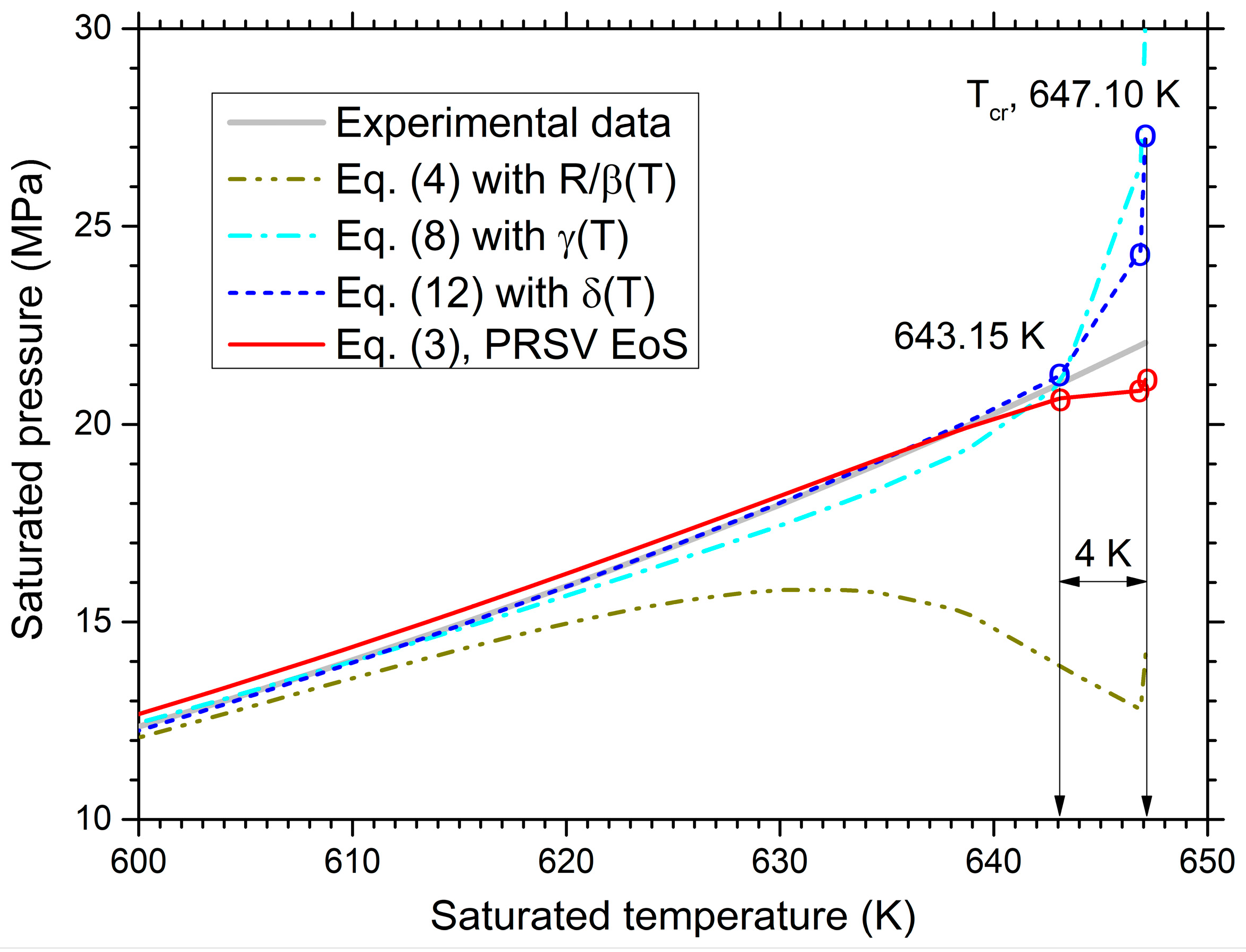
T_sat and their corresponding P_sat ranges provided by ASME Steam Tables are 273.16 to 647.10 K and 0.000612 to 22.064 MPa, respectively. This range was selected because it represents the complete saturated-vapor temperature range used for developing and assessing the proposed correction functions. Since the variation in P_sat with respect to T_sat is extremely wide, it would be visually unclear to compare the calculated and experimental pressures in a single graph. Therefore, the comparison is systematically divided into several temperature ranges. Figure 6 and Figure 7 show P_sat calculated using the corrected ideal gas law, along with the corresponding experimental data from 273.16 K to the critical point of steam. The corrected ideal gas laws are given by Equations (4), (8), and (12).

Figure 6. Comparison of the experimentally measured P_sat of steam with respect to T_sat over the range from 273.16 K to 647.10 K. The calculated values are obtained using Equations (4), (8), (12), as well as the PRSV EoS. The experimental saturated-pressure data were taken from the ASME Steam Tables [43]. (a) T_s: 273.16 K to 300 K. (b) T_s: 300 K to 350 K. (c) T_s: 350 K to 400 K. (d) T_s: 400 K to 450 K. (e) T_s: 450 K to 550 K. (f) T_s: 550 K to 647.1 K.

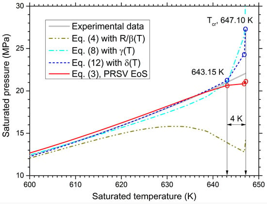
Figure 7. Comparison of P_sat of steam with respect to T_sat over the range from 600 K to 647.10 K, i.e., near the critical point. The calculated values are obtained using Equations (4), (8), (12), as well as the PRSV EoS. The experimental saturated-pressure data were taken from the ASME Steam Tables [43]. The ideal gas laws incorporating the coefficients, which approximate the corrected specific gas constant R_corr, are given by Equations (4), (8), and (12). These equations have more compact analytical forms than the RK EoS or the PRSV EoS and can be evaluated directly once the gas-specific fitting parameters are available. The RK EoS serves as the foundation for the PRSV EoS because the PRSV was developed via the SRK EoS, which is a modification of the RK EoS. To date, the PRSV EoS has been widely regarded as one of the most accurate EoS among the existing models.

Although Equations (4), (8), and (12) are based on the ideal gas law, the results calculated using these equations exhibit excellent agreement with the experimental data over most of T_sat range, except near the critical point, and are sufficiently comparable to those obtained from the more complex PRSV EoS, as shown in Figure 6 and Figure 7. However, the agreement deteriorates as T_sat approaches the critical point. Therefore, the near-critical region is treated separately in the following analysis, and the proposed correlation should not be regarded as reliable in the immediate vicinity of the critical point.

In the case of Equation (4), as shown in Figure 2, the correction factor of R/β(T) shows relatively large deviations at low temperatures and near the critical point. The error remains within approximately ±3% up to 608 K. As the temperature approaches the critical point, the errors increase sharply in the negative direction as illustrated in Figure 7. This suggests that, despite the simplicity of Equation (4), the magnitude of these errors limits its suitability for use in engineering applications.

In the case of Equation (8), the correction factor γ(T) also shows some deviation in both the low- and high- temperature regions near the critical point. However, compared with Equation (4), it exhibits significantly reduced errors overall. The deviation from the experimental data remains consistently within ±3.2% except for the last two points (at 646.86 K and 647.10 K). These two points, which include the critical point, show the errors of +20.7% and +37.7%, respectively. Therefore, Equation (8) can be satisfactorily used to predict P_sat, provided that it is not applied in the immediate vicinity of the critical point.

In the case of Equation (12), P_sat are calculated within the error range of ±2.6% over the entire temperature range, except for the last two points. The errors exceeding ±2.6% are observed only in the very narrow range from 628 K to 639 K. However, at 646.86 K and 647.10 K, the deviations from the experimental data are +10.8% and +24.58%, respectively. Excluding the immediate vicinity of the critical point, P_sat values calculated from Equation (12) agree well with the experimental data within the fitted saturated-vapor range, showing a level of accuracy comparable to PRSV EoS results. Considering its compact analytical form, Equation (12) allows direct evaluation for repeated engineering calculations.

To provide a quantitative comparison of the candidate correction functions and the PRSV EoS, the root mean square error (RMSE) and maximum absolute pressure deviations were calculated for each model. For a consistent comparison, all models were evaluated at the same 165 saturated-vapor states using the same experimental T_sat and v_sat values from the ASME Steam Tables, and the calculated P_sat values were compared with the same experimental P_sat values using an identical error definition.

The pressure deviation at each temperature point was evaluated as ε = (P_cal − P_exp)/P_exp × 100. The statistical results are summarized in Table 1 for both the full saturated-vapor data range and the range excluding the last two near-critical points. In Table 1, the two evaluation ranges were reported to distinguish the overall performance over the full saturated-vapor range from the behavior in the immediate near-critical region, where empirical correlations and cubic EoSs commonly exhibit increased deviations.

Table 1. RMSE and maximum absolute pressure deviations for the candidate correlations and the PRSV EoS.

Model/Correlation	RMSE, Full Range (%)	Maximum Error, Full Range (%)	RMSE, Excluding Two Near-Critical Point (%)	Maximum Error, Excluding Two Near Critical Point (%)
Equation (4), R/β(T)	7.5906	41.8769	6.3056	34.1651
Equation (8), γ(T)	3.5389	37.6723	1.1620	3.3206
Equation (12), δ(T)	2.7122	24.5768	1.7382	2.6769
Equation (3), PRSV	1.8478	5.2049	1.7833	2.7867

As shown in Table 1, the maximum errors of all correlations increase significantly when the last two near-critical points are included. When these two points are excluded, Equation (12) shows the lowest maximum absolute error among the proposed correlations, while the RMSE values of Equation (8), Equation (12), and the PRSV EoS are comparable. These results support the engineering applicability of the proposed correlation within the saturated-vapor region, while also confirming its reduced reliability near the critical point.

In addition to the accuracy comparison, the intended use of the proposed correlation was further clarified from the viewpoint of repeated property evaluation. The proposed correlation allows the saturated pressure to be evaluated directly using an analytical temperature-dependent fitting function in the ideal-gas-form expression. In contrast, a pre-tabulated compressibility-factor approach requires storage of tabulated values and interpolation at each target temperature.

A reference-property package based on a thermodynamically consistent reference EoS, such as REFPROP or CoolProp, provides broader thermodynamic consistency and applicability, but it generally involves more complex property routines than the direct analytical correlations used in this study. These implementation characteristics are summarized in Table 2. However, no execution-time benchmark was performed in this study; therefore, the present comparison concerns algebraic and implementation simplicity rather than a quantitatively demonstrated computational speed advantage.

Table 2. Qualitative comparison of implementation characteristics for repeated saturated-vapor P-v-T evaluation.

Method	Required Procedure	Interpolation Required	Accuracy Basis	Main Limitation
Present Rcorr correlation	Direct evaluation of an analytical temperature-dependent fitting function and the ideal-gas-form equation	No	Empirical fit to saturated-vapor P-v-T data	Limited to the fitted saturated-vapor range
Pre-tabulated compressibility-factor approach	Lookup of tabulated compressibility-factor values and interpolation at the target temperature	Yes	Depends on tabulated data and interpolation interval	Requires tabulated data and an interpolation scheme

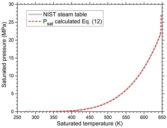
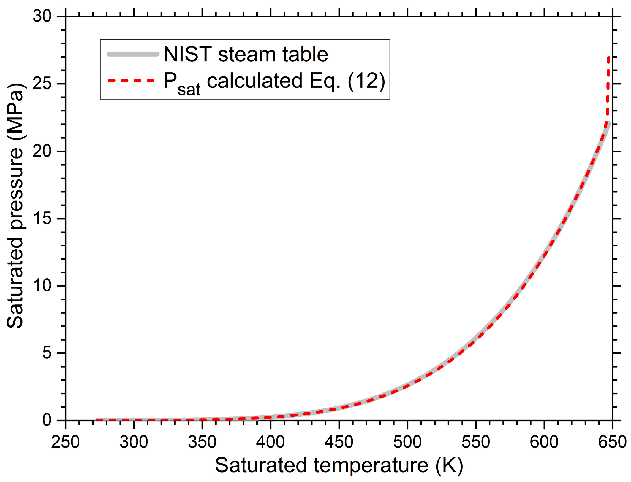
To further assess the applicability of Equation (12), a cross-dataset reference comparison was conducted using 375 saturation-state points reported in National Institute of Standards and Technology Interagency/Internal Report (NISTIR) 5078 over the temperature range of 273.16–647.096 K, including the critical point. The NIST dataset was generated using the IAPWS-95 reference formulation and was not used in the development or parameter estimation of Equation (12). Therefore, this comparison should not be interpreted as validation against independent raw experimental measurements.

As shown in Figure 8, the calculated saturation pressures agree closely with the corresponding NIST values over most of the investigated range. The RMSE of the relative deviations was 2.1462% for the complete dataset, while the maximum absolute relative deviation of 24.59% occurred at the critical point. When the three highest-temperature points at 645.16, 646.16, and 647.096 K were excluded as a supplementary assessment of the influence of the immediate near-critical region, the RMSE decreased to 1.7202%. Nevertheless, all 375 data points, including the critical point, were retained in the principal cross-dataset assessment. This comparison evaluates the transferability of Equation (12) to a separate reference dataset without refitting, rather than providing independent experimental validation.

Figure 8. Cross-dataset comparison of Equation (12) against NISTIR 5078: comparison of the reported and calculated saturation pressures and the corresponding relative deviations over the temperature range of 273.16–647.096 K, including the critical point.

4.2. Comparison of the Specific Volumes

As previously mentioned, according to the State Postulate [44,45,46,47], the state of a simple compressible system is completely specified by two independent intensive properties. However, because the pressure calculated from Equation (12) is substituted back into the same relation to determine the specific volume, this procedure is algebraically dependent and does not constitute an independent validation of the specific volume. The comparison presented in this subsection is therefore intended only to illustrate the internal consistency of the calculation and to provide a reference comparison with the PRSV EoS.

Because Equation (12) is used to calculate P_sat and, after rearrangement, to recover the specific volume, the resulting specific-volume agreement is algebraically constrained and does not provide an independent accuracy assessment. By contrast, the PRSV EoS requires solving the cubic equation given by Equation (13) to obtain the specific volume.

$$P={\displaystyle \frac{RT\left(v^2+2bv-b^2\right)-a\left(v-b\right)}{\left(v-b\right)\left(v^2+2bv-b^2\right)}},$$

$$RT\left(v^2+2bv-b^2\right)-a\left(v-b\right)-P\left(v-b\right)\left(v^2+2bv-b^2\right)=0,$$

$$v^3+\left(b-{\displaystyle \frac{RT}{P}}\right)v^2-\left(3b^2+{\displaystyle \frac{2RTb}{P}}-{\displaystyle \frac{a}{P}}\right)v+\left(b^3+{\displaystyle \frac{RT{b}^2}{P}}-{\displaystyle \frac{ab}{P}}\right)=0,$$

(13)

where the coefficients of Equation (13) are the same as those in Equation (3). Since the coefficients of a and b contain the complex sub-coefficients, solving Equation (13) analytically using Cardano’s formula [48,49] is highly cumbersome and nearly infeasible. Therefore, computer-based numerical analysis is the most appropriate method. In this study, Equation (13) was solved by the np.root ( ) function provided by Python (version 3.11.1). The Python code used in this study is included in Appendix A.1 for reference.

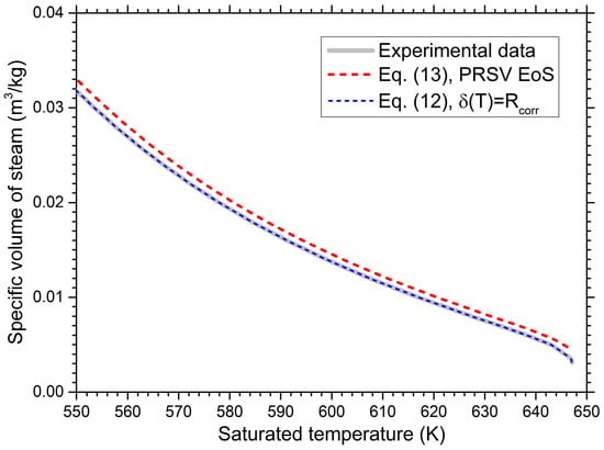
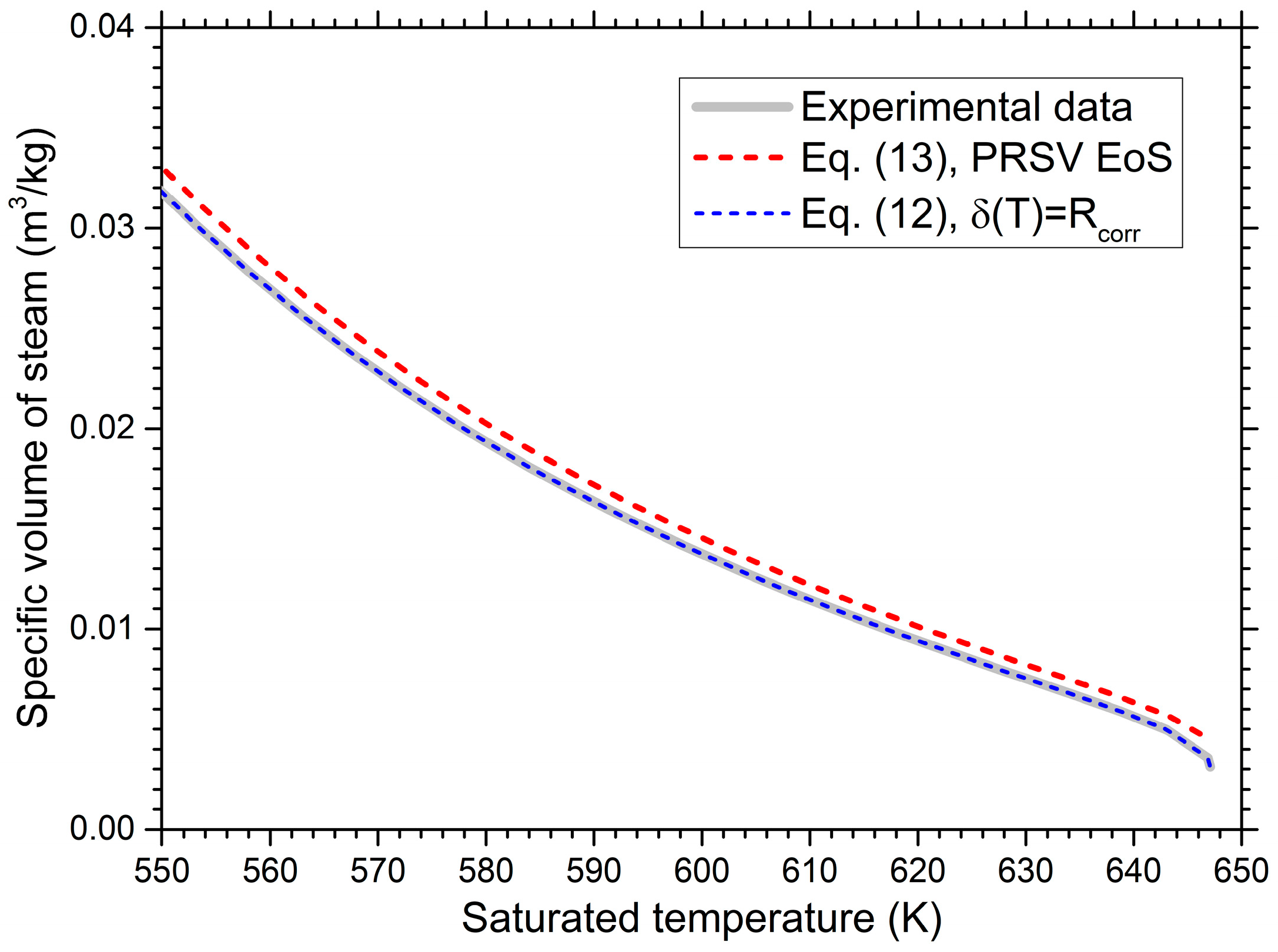
Figure 9 compares the experimentally measured saturated-vapor specific volume of steam with the values obtained from Equation (12) and the PRSV EoS from 550 K to the critical point. The PRSV EoS slightly overestimates the experimental specific volume from the low-temperature region, and the deviation increases progressively as the temperature approaches the critical point. A similar increase in specific-volume deviation at elevated temperatures and pressures was reported by Choi et al. [30] for the vdW and RK EoSs. In contrast, Equation (12) closely reproduces the experimental values; however, this agreement is algebraically constrained and should not be interpreted as independent validation.

Figure 9. Comparison of the experimentally measured saturated-vapor specific volume of steam with the values calculated using Equation (12) and the PRSV EoS over the range from 550 K to 647.1 K. The experimental data were taken from the ASME Steam Tables [43].

Therefore, the apparent agreement of the specific volume obtained from Equation (12) should not be interpreted as independent evidence of predictive accuracy or superiority over the PRSV or other EoSs.

In Equation (12), the specific volume is calculated using the pressure value obtained from the corrected specific gas constant expressed in the form of an elliptical equation, which introduces some error. However, this pressure containing an error is subsequently used in the denominator to calculate the specific volume. Therefore, since the errors are effectively cancelled out in the denominator and the numerator, the specific volume shows no apparent deviation from the experimental data.

5. Validity of the Ideal Gas Law with the Approximated Corrected Specific Gas Constant

In the preceding section, the approximated corrected specific gas constant R_corr was applied to saturated steam to assess the proposed methodology within a gas-specific case. It should be emphasized that this assessment is limited to a gas-specific case and does not imply universal applicability. However, to further examine the applicability of the proposed gas-specific correction framework, it is necessary to apply the methodology to other real gases with distinct molecular characteristics. In this section, the elliptically approximated R_corr given by Equation (12) is examined for methane (CH₄), not as a universal correction but as a test case to assess how the functional form of R_corr depends on the nature of the gas.

Water is a typical polar substance; it is also an asymmetric, polyatomic molecule that forms strong hydrogen bonds. These molecular characteristics make it difficult to accurately calculate its thermophysical properties using equations of state [50]. On the other hand, methane is a non-polar, symmetric, polyatomic molecule, and its thermodynamic properties can be adequately predicted within the range of engineering applications, even by a simple EoS [51]. Nevertheless, the applicability of the ideal gas law employing an approximated corrected specific gas constant to methane cannot be assumed a priori, because it depends strongly on the temperature-dependent shape of R_corr. In other words, the validity of the proposed approach for a given gas is governed by how well the selected functional form represents the experimentally derived variation of R_corr.

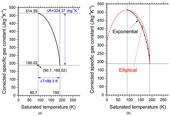
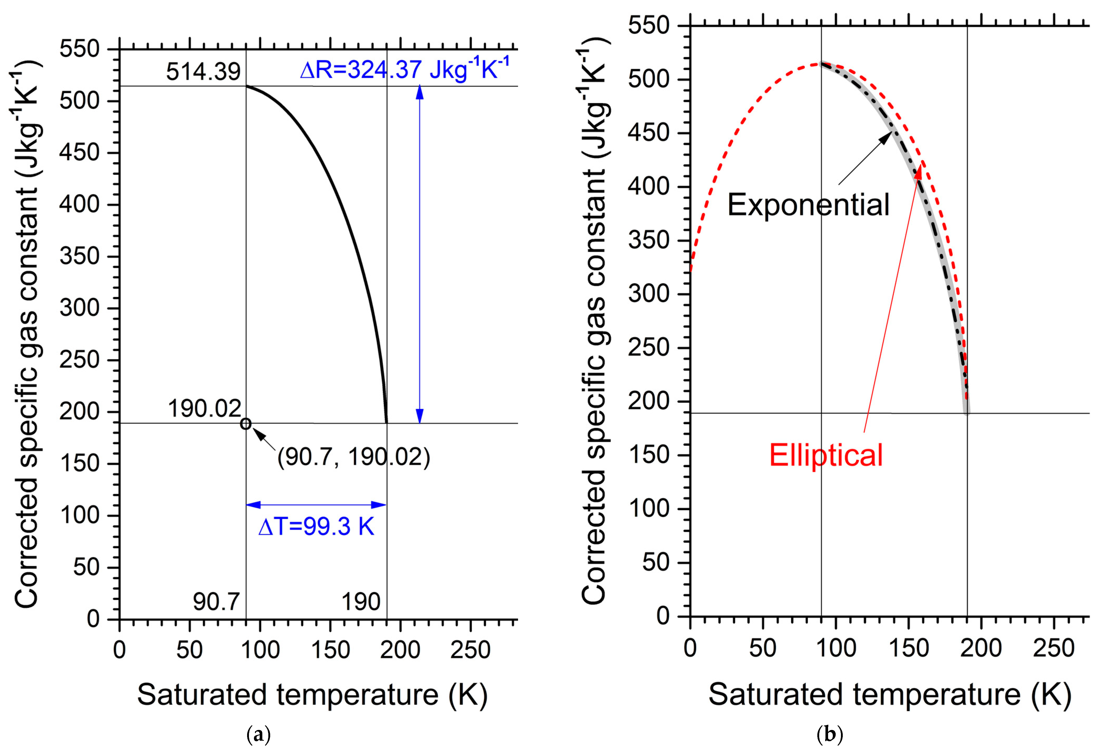
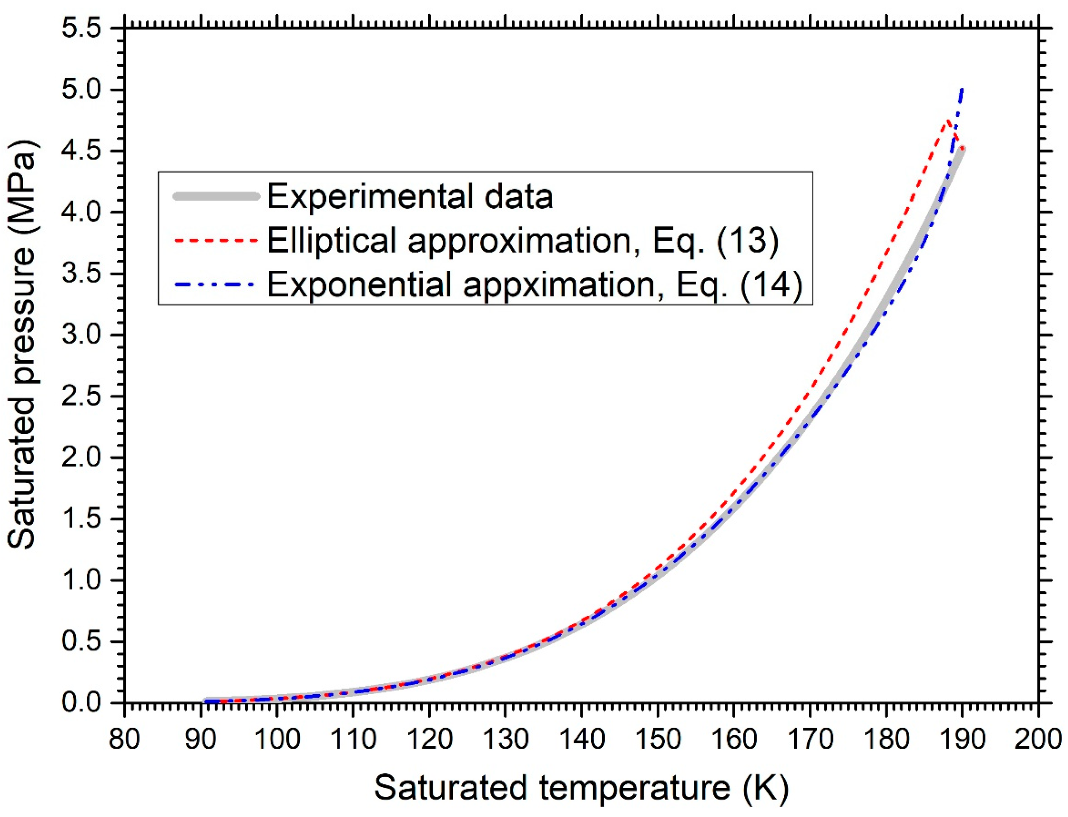
To further examine the proposed framework using methane as an additional test case, the experimental data for methane were obtained from ASTM D-3956-12, titled Standard Specification for Methane Thermophysical Property Tables, published by the American Society for Testing and Materials (ASTM) [52], the table of which is listed in Appendix A.2. Figure 10a shows the plot for R_corr of methane on a graph with equal scale intervals on both axes. Unlike saturated steam, a sharp curvature near 90 K is observed in the graph. Therefore, if R_corr is approximated using the elliptical equation given in Equation (11), non-negligible errors are expected due to this sharp curvature. According to the comparison between the experimental and calculated pressures, Equation (14) exhibits a maximum deviation of +12.42% at 186 K compared with the experimental data.

$$R_{ellip}=190.02+324.37\sqrt{ \left[1-{\displaystyle \frac{{\left(T-90.7\right)}^2}{{\left(99.3\right)}^2}}\right] }.$$

(14)

Figure 10. Corrected specific gas constant of methane and its approximations. The corrected specific gas constant R_corr is more suitably approximated by an exponential function than by an elliptical equation. (a) Corrected specific gas constant of methane, R_corr. (b) Comparison of R_corr with the exponential and elliptical approximations. The gray line in (b) represents R_corr.

Figure 10b compares the curves fitted by Equation (14) based on the elliptical approximation and Equation (15), which adopts an exponential functional form for methane; the elliptical and exponential functions were quantitatively compared using the RMSE and maximum absolute relative pressure deviation. Over the full dataset, the RMSE values were 6.43% and 1.85% for the elliptical and exponential functions, respectively. Therefore, the exponential function was selected as the more appropriate representation of R_corr for methane. It is evident that, for methane, the exponential function provides a more appropriate representation of R_corr than the elliptical equation, owing to the sharp curvature observed in its temperature dependence. This result indicates that no single functional form can universally approximate R_corr across different gases and that the selection of the approximation function must be gas-specific. Accordingly, the exponential function adopted for methane is given by Equation (15).

$$R_{expo}=535.69863-1.75263\times e^{0.02748T}.$$

(15)

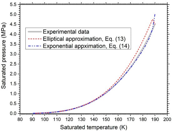
Figure 11 shows the saturated pressures from the experimental data and those calculated using the two corrected specific gas constants of R_ellip and R_expo, simultaneously. When the ideal gas law employing R_expo is used to calculate the saturated pressure, the errors from the experimental data fall within about ±2% over the entire temperature range, except at the highest-temperature near-critical point of 190 K. At this point, the deviation in the saturated pressure is approximately +11%. The ASTM data used here extend to 190 K, slightly below the methane critical temperature; therefore, the exact critical point is not included in the present fitting dataset.

Figure 11. Comparison of the experimentally measured P_sat of methane with the calculated results obtained from Equations (14) and (15), which represent the elliptical and exponential approximations of the corrected specific gas constant, respectively. The experimental saturated-vapor properties of methane were obtained from Refs. [51,52,53,54].

6. Discussion

In this study, the specific gas constant was corrected, as shown in Equation (7), to match the calculation results obtained from the ideal gas law with the experimental data. The corrected value was subsequently approximated using an appropriate mathematical function over the temperature range covered by the experimental property tables. Although the fitted function is referred to as the corrected specific gas constant R_corr, it should be emphasized that it does not redefine the intrinsic gas constant. Rather, R_corr should be interpreted as a temperature-dependent fitting parameter with the same units as R, introduced to reduce the deviation between ideal-gas predictions and experimental saturated-vapor P-v-T data.

To clarify the thermodynamic meaning of R_corr, it is useful to compare it with the compressibility factor Z. The compressibility factor Z is a dimensionless quantity that indicates the degree of deviation a real gas from ideal gas behavior, and it is defined as

$$Z={\displaystyle \frac{Pv}{RT}}.$$

(16)

For the saturated-vapor P-v-T data considered in this study, substituting the corrected ideal-gas-form relation P = γ(T)T/v, where γ(T) corresponds to the fitted form of R_corr, into Equation (16) gives

$$Z_{sat}(T)={\displaystyle \frac{R}{R_{corr}}}.$$

(17)

Equation (17) shows that, along the saturated-vapor line, R_corr(T)/R is algebraically equivalent to the compressibility factor Z_sat(T). Therefore, the present formulation should not be interpreted as introducing a new thermodynamic quantity distinct from the compressibility factor. Its intended contribution is practical: R_corr(T) provides a gas-specific analytical representation of saturation-line nonideality while retaining the simple ideal-gas-form expression for repeated engineering calculations.

If the values of P-v-T are experimental data, Z indicates how closely a real gas follows the ideal gas law. However, if two of these variables are obtained from experimental data and the remaining variable is calculated, Z reflects the accuracy with which a given equation of state represents real-gas behavior. If Equation (16) is used to calculate the pressure, the pressure is expressed as

$$P=Z{\displaystyle \frac{RT}{v}}.$$

(18)

The compressibility factor Z can be expanded using the Virial coefficients [26] as shown in

$$Z=1+{\displaystyle \frac{B_2}{v}}+{\displaystyle \frac{B_3}{v^2}}+{\displaystyle \frac{B_4}{v^3}}+\dots \mathrm{or}$$

(19)

$$Z=1+B_2^{\prime }P+B_3^{\prime }{P}^2+B_4^{\prime }{P}^3+\dots .$$

(20)

The Virial coefficients B_n and B_n’ correspond to the expansions in reciprocal specific volume and pressure, respectively, and can be determined experimentally or theoretically. In the experimental method, the compressibility factor Z is first evaluated from the measured values of P-v-T. If Z is plotted with respect to the pressure P or the reciprocal of the specific volume 1/v, it can be approximated in the form of Equations (19) or (20).

In contrary, the theoretical determination of the Virial coefficients involves performing complex integrals. For instance, the second Virial coefficient B₂ in Equation (19) is calculated from the integration of

$$B_2=-2\pi N_A{\displaystyle {\int }_0^{\infty }\left[e^{-\frac{U\left(r\right)}{k T}}-1\right]} r^2 dr,$$

(21)

where N_A is Avogadro’s number, U(r) is the intermolecular potential depending on the intermolecular distance r, and k is the Boltzmann constant [55,56,57,58]. The analytical integration of Equation (21) is very difficult even for the simplest case of the Lennard–Jones potential [59]. In the case of high-order Virial coefficients, the theoretical calculations become more complicated because they involve multiple integrals of the corresponding intermolecular forces with respect to the intermolecular distance [59,60].

Accordingly, in comparison with both the experimental and theoretical procedures required to determine Virial coefficients, the present approach provides a simpler empirical way to reduce the deviation of the ideal gas law for the saturated P-v-T data. It should be noted that this approach does not replace the formal Virial expansion or existing equations of state but provides a gas-specific, temperature-dependent fitting framework that is particularly suitable for engineering calculations in the saturated-vapor region considered in this study.

It should also be emphasized that the present correlation is not a fundamental equation of state. Since the proposed formulation is based on a single empirical temperature-dependent fitting parameter, it is intended only for the representation of saturated-vapor P-v-T data considered in this study. Therefore, it does not provide a thermodynamically complete framework for deriving caloric properties such as enthalpy, entropy, heat capacity, or speed of sound through Maxwell relations. For applications requiring a thermodynamically consistent set of properties, established reference equations of state or validated multiparameter property formulations should be used.

7. Conclusions

The development of gas equations began with the fundamental relationships reported by Boyle [61] and Gay-Lussac [62], followed by the ideal gas law formalized by Clapeyron [63,64]. Subsequently, the van der Waals equation provided a major extension of the ideal gas law to real-gas behavior [23,24,25,26].

More advanced EoSs, including the RK and PRSV models, were developed to improve real-gas predictions. In contrast, the present study adopts a data-driven approach in which a temperature-dependent fitting parameter, R_corr, is introduced into the ideal-gas form using experimental saturated-vapor P-v-T data.

The corrected specific gas constant R_corr = Pv/T is evaluated from experimentally measured P-v-T data. It is a gas-specific, temperature-dependent fitting parameter with the same units as R, rather than as a redefinition of the physical constant. Subsequently, the corrected specific gas constant was fitted using a gas-specific function selected from the observed R_corr trend. The proposed correlation is intended only for saturated-vapor P-v-T evaluation and should not be interpreted as a universal or thermodynamically complete equation of state.

The corrected specific gas constant R_corr was approximated using rational, exponential, and elliptical functions. The elliptical form agreed well with the steam data, with smaller deviations than the PRSV EoS in some temperature ranges. The framework was also examined for methane. The results demonstrate the feasibility of the proposed framework for methane as an additional gas-specific case; however, they are insufficient to establish broader applicability to other gases.

Overall, the findings of this study indicate that the corrected specific gas constant serves as a gas-specific, temperature-dependent fitting parameter for reducing the deviation of the ideal-gas form within the saturated-vapor P-v-T region considered in this study. Rather than offering a universal modification, the proposed methodology provides a gas-specific empirical framework. Its applicability to additional real gases should be evaluated individually using reliable saturated-vapor data, and further studies involving a broader range of gases are required before general applicability can be established. The proposed framework is intended for repeated saturated-vapor P-v-T evaluations in engineering applications. Because R_corr is gas-specific and derived from experimental data, each gas requires its own fitting function and coefficients; therefore, the method should be regarded as an empirical correlation rather than a universal predictive model.

For reproducibility, the procedure used in this study can be summarized as follows: (1) obtain saturated-vapor P-v-T data from the cited reference source; (2) calculate R_corr = Pv/T at each saturation state using Equation (7); (3) fit candidate functions to the temperature dependence of R_corr and evaluate them using RMSE and maximum absolute relative pressure deviation; (4) substitute the selected fitting function into the ideal-gas-form equation to calculate P_sat; and (5) assess the resulting correlation using the development dataset and, where available, a separate reference dataset without refitting.

Appendix A.1. Python Code for Solving the PRSV Cubic Equation

Python code for solving Equation (13), a cubic equation: In the code, Tr denotes the reduced temperature, and vs is the specific volume of steam at a given saturated state. Since Equation (13) may yield up to three real roots, the largest real root is selected as the saturated-vapor specific volume.

01 import numpy as np

02 # Input of saturated pressure and saturated temperature

04 P = 0.000612e6

05 T = 273.16

06

07 # Critical properties of steam: No changes hereinafter.

08 Pcr = Pcr = 22.064e6

09 Tcr = 647.096

10

11 # Coefficients of the PRSV EoS.

12 R = 461.521

13 b = 0.077796*R*Tcr/Pcr

14 w = 0.34380

15 k0 = 0.378893 + 1.4897153*w - 0.17121848*w**2 + 0.0196554*w**3

16 k1 = −0.06635

17 Tr = T/Tcr

18 k = k0 + k1*(1 + Tr**0.5)*(0.7 - Tr)

19 alpha = (1 + k*(1 - Tr**0.5))**2

20 a = 0.457235*R**2*Tcr**2/Pcr*alpha

21

22 # Coefficients of the cubic equation.

23 v3 = 1

24 v2 = b - R*T/P

25 v1 = -(3*b**2 + 2*R*T*b/P - a/P)

26 v0 = b**3 + R*T*b**2/P - a*b/P

27

28 # Solution of the cubic equation.

29 coeff = [v3, v2, v1, v0]

30 vs = np.roots(coeff)

31

32 print(vs)

Appendix A.2. Methane Saturation-Property Data

Table A1 lists the thermodynamic properties of methane at liquid–vapor equilibrium. In the original dataset, the densities of the saturated liquid and vapor are given in units of mol/liter; however, they have been converted to units of m³/kg in this study.

In Table A1, the saturated temperature of 112 K corresponds to a saturated pressure slightly above atmospheric pressure, which is shaded with background color. The highest-temperature datum in the ASTM dataset is 190 K, which is slightly below the critical temperature of methane (T_cr ≈ 190.56 K). Therefore, this datum is treated as a near-critical point rather than the exact critical point, and the saturated-liquid and saturated-vapor specific volumes are not expected to be identical at 190 K [51]. The last column of Table 1 lists the corrected specific gas constant calculated from R = Pv/T in which P-v-T are the measured experimental data. Since the theoretical specific gas constant of methane is 518.2705 J/kg∙K [52], the corrected specific gas constant serves as a bridge that enables the ideal gas law to be applied to the real gas, methane.

Table A1. Standard specification for methane thermophysical properties.

T (°C)	T (K)	P (Mpa)	vL (m3/kg)	vG (m3/kg)	Rcorr
−182.45	90.7	0.011705	0.002215	3.985943	514.393
−181.15	92	0.013801	0.002224	3.425690	513.891
−179.15	94	0.017613	0.002237	2.737995	513.025
−177.15	96	0.022233	0.002251	2.210942	512.040
−175.15	98	0.027778	0.002265	1.802531	510.926
−173.15	100	0.034376	0.002279	1.482690	509.690
−171.15	102	0.042160	0.002293	1.229789	508.313
−169.15	104	0.051275	0.002308	1.027950	506.809
−167.15	106	0.061868	0.002323	0.865482	505.148
−165.15	108	0.074099	0.002339	0.733633	503.347
−163.15	110	0.088130	0.002355	0.625807	501.385
−161.15	112	0.10413	0.002371	0.536987	499.254
−159.15	114	0.12228	0.002387	0.463353	497.007
−157.15	116	0.14275	0.002405	0.401857	494.527
−155.15	118	0.16574	0.002422	0.350228	491.922
−153.15	120	0.19143	0.002440	0.306631	489.153
−151.15	122	0.22002	0.002459	0.269596	486.201
−149.15	124	0.25170	0.002478	0.237982	483.065
−147.15	126	0.28667	0.002497	0.210857	479.733
−145.15	128	0.32514	0.002517	0.187479	476.226
−143.15	130	0.36732	0.002538	0.167241	472.546
−141.15	132	0.41341	0.002560	0.149643	468.666
−139.15	134	0.46363	0.002582	0.134281	464.602
−137.15	136	0.51819	0.002605	0.120820	460.351
−135.15	138	0.57730	0.002629	0.108976	455.883
−133.15	140	0.64118	0.002654	0.098523	451.221
−131.15	142	0.71006	0.002680	0.089263	446.353
−129.15	144	0.78415	0.002707	0.081035	441.275
−127.15	146	0.86368	0.002735	0.073699	435.975
−125.15	148	0.94887	0.002764	0.067140	430.454
−123.15	150	1.0400	0.002795	0.061260	424.736
−121.15	152	1.1372	0.002827	0.055964	418.699
−119.15	154	1.2408	0.002861	0.051194	412.477
−117.15	156	1.3509	0.002896	0.046879	405.954
−115.15	158	1.4680	0.002934	0.042963	399.175
−113.15	160	1.5921	0.002974	0.039406	392.114
−111.15	162	1.7235	0.003016	0.036160	384.702
−109.15	164	1.8626	0.003016	0.033194	376.995
−107.15	166	2.0096	0.003111	0.030473	368.907
−105.15	168	2.1647	0.003164	0.027971	360.410
−103.15	170	2.3283	0.003221	0.025662	351.464
−101.15	172	2.5007	0.003284	0.023526	342.043
−99.15	174	2.6822	0.003353	0.021540	332.038
−97.15	176	2.8732	0.003431	0.019685	321.358
−95.15	178	3.0740	0.003519	0.017944	309.887
−93.15	180	3.2852	0.003621	0.016296	297.420
−91.15	182	3.5071	0.003741	0.014722	283.690
−89.15	184	3.7405	0.003890	0.013193	268.198
−87.15	186	3.9860	0.004084	0.011670	250.089
−85.15	188	4.2448	0.004369	0.010064	227.232
−83.15	190	4.5186	0.004982	0.007990	190.019

Table A1. Standard specification for methane thermophysical properties.

T (°C)	T (K)	P (Mpa)	vL (m3/kg)	vG (m3/kg)	Rcorr
−182.45	90.7	0.011705	0.002215	3.985943	514.393
−181.15	92	0.013801	0.002224	3.425690	513.891
−179.15	94	0.017613	0.002237	2.737995	513.025
−177.15	96	0.022233	0.002251	2.210942	512.040
−175.15	98	0.027778	0.002265	1.802531	510.926
−173.15	100	0.034376	0.002279	1.482690	509.690
−171.15	102	0.042160	0.002293	1.229789	508.313
−169.15	104	0.051275	0.002308	1.027950	506.809
−167.15	106	0.061868	0.002323	0.865482	505.148
−165.15	108	0.074099	0.002339	0.733633	503.347
−163.15	110	0.088130	0.002355	0.625807	501.385
−161.15	112	0.10413	0.002371	0.536987	499.254
−159.15	114	0.12228	0.002387	0.463353	497.007
−157.15	116	0.14275	0.002405	0.401857	494.527
−155.15	118	0.16574	0.002422	0.350228	491.922
−153.15	120	0.19143	0.002440	0.306631	489.153
−151.15	122	0.22002	0.002459	0.269596	486.201
−149.15	124	0.25170	0.002478	0.237982	483.065
−147.15	126	0.28667	0.002497	0.210857	479.733
−145.15	128	0.32514	0.002517	0.187479	476.226
−143.15	130	0.36732	0.002538	0.167241	472.546
−141.15	132	0.41341	0.002560	0.149643	468.666
−139.15	134	0.46363	0.002582	0.134281	464.602
−137.15	136	0.51819	0.002605	0.120820	460.351
−135.15	138	0.57730	0.002629	0.108976	455.883
−133.15	140	0.64118	0.002654	0.098523	451.221
−131.15	142	0.71006	0.002680	0.089263	446.353
−129.15	144	0.78415	0.002707	0.081035	441.275
−127.15	146	0.86368	0.002735	0.073699	435.975
−125.15	148	0.94887	0.002764	0.067140	430.454
−123.15	150	1.0400	0.002795	0.061260	424.736
−121.15	152	1.1372	0.002827	0.055964	418.699
−119.15	154	1.2408	0.002861	0.051194	412.477
−117.15	156	1.3509	0.002896	0.046879	405.954
−115.15	158	1.4680	0.002934	0.042963	399.175
−113.15	160	1.5921	0.002974	0.039406	392.114
−111.15	162	1.7235	0.003016	0.036160	384.702
−109.15	164	1.8626	0.003016	0.033194	376.995
−107.15	166	2.0096	0.003111	0.030473	368.907
−105.15	168	2.1647	0.003164	0.027971	360.410
−103.15	170	2.3283	0.003221	0.025662	351.464
−101.15	172	2.5007	0.003284	0.023526	342.043
−99.15	174	2.6822	0.003353	0.021540	332.038
−97.15	176	2.8732	0.003431	0.019685	321.358
−95.15	178	3.0740	0.003519	0.017944	309.887
−93.15	180	3.2852	0.003621	0.016296	297.420
−91.15	182	3.5071	0.003741	0.014722	283.690
−89.15	184	3.7405	0.003890	0.013193	268.198
−87.15	186	3.9860	0.004084	0.011670	250.089
−85.15	188	4.2448	0.004369	0.010064	227.232
−83.15	190	4.5186	0.004982	0.007990	190.019

References

- Lim, J.T.; Habibullah, A.; Ng, E.Y.K. Towards a Digital Twin for Gas Turbines: Thermodynamic Modeling, Critical Parameter Estimation, and Performance Optimization Using PINN and PSO. Energies 2025, 18, 3721. [Google Scholar] [CrossRef] [Scilit]
- Patorkin, D.; Kindra, V.; Vegera, A.; Pisarev, D.; Malenkov, A. Design of Heat Exchangers with Low-Boiling Working Fluids: Algorithm Development and Parameter Optimization. Energies 2025, 18, 5987. [Google Scholar] [CrossRef] [Scilit]
- Wang, H.; Liu, H.; Ma, T.; Xie, T.; Wang, T.; Yang, R.; Wang, Y.; Zhai, P.; Yu, L.; Jing, X. Numerical study on flow and temperature rise characteristics of low-pressure cylinder of steam turbine under variable working conditions. J. Phys. Conf. Ser. 2025, 2992, 012044. [Google Scholar] [CrossRef] [Scilit]
- Chen, C.; Liu, M.; Li, M.; Wang, Y.; Wang, C.; Yan, J. Digital twin modeling and operation optimization of the steam turbine system of thermal power plants. Energy 2024, 290, 129969. [Google Scholar] [CrossRef] [Scilit]
- Motamed, M.A.; Genrup, M.; Nord, L.O.; Genrup, M.; Nord, L.O. Part-load thermal efficiency enhancement in gas turbine combined cycles by exhaust gas recirculation. Appl. Therm. Eng. 2024, 244, 122716. [Google Scholar] [CrossRef] [Scilit]
- Hornung, A.; Jahangiri, H.; Ouadi, M.; Kick, C.; Deinert, L.; Meyer, B.; Grunwald, J.; Daschner, R.; Apfelbacher, A.; Meiller, M.; et al. Thermo-Catalytic Reforming (TCR)–An important link between waste management and renewable fuels as part of the energy transition. Appl. Energy Combust. Sci. 2022, 12, 100088. [Google Scholar] [CrossRef] [Scilit]
- Akerboom, S.; Waldmann, S.; Mukherjee, A.; Agaton, C.; Sanders, M.; Kramer, G.J. Different this time? The prospects of CCS in the Netherlands in the 2020s. Front. Energy Res. 2021, 9, 644796. [Google Scholar] [CrossRef] [Scilit]
- Alabdullah, M.A.; Gomez, A.R.; Vittenet, J.; Bendjeriou-Sedjerari, A.; Xu, W.; Abba, I.A.; Gascon, J. A viewpoint on the refinery of the future: Catalyst and process challenges. ACS Catal. 2020, 10, 8131–8140. [Google Scholar] [CrossRef] [Scilit]
- Joung, T.H.; Kang, S.G.; Lee, J.K.; Ahn, J. The IMO initial strategy for reducing Greenhouse Gas (GHG) emissions, and its follow-up actions towards 2050. J. Int. Marit. Saf. Environ. Aff. Shipp. 2020, 4, 1–7. [Google Scholar] [CrossRef] [Scilit]
- Zhang, C.; Zhu, J.; Guo, H.; Xue, S.; Wang, X.; Wang, Z.; Chen, T.; Yang, L.; Zeng, X.; Su, P. Technical requirements for 2023 IMO GHG strategy. Sustainability 2024, 16, 2766. [Google Scholar] [CrossRef] [Scilit]
- Deng, S.; Mi, Z. A review on carbon emissions of global shipping. Mar. Dev. 2023, 1, 4. [Google Scholar] [CrossRef] [Scilit]
- Jimenez, V.J.; Kim, H.; Munim, Z.H. A review of ship energy efficiency research and directions towards emission reduction in the maritime industry. J. Clean. Prod. 2022, 366, 132888. [Google Scholar] [CrossRef] [Scilit]
- Chun, K.W.; Kim, M.; Hur, J.-J. Development of a marine LPG-fueled high-speed engine for electric propulsion systems. J. Mar. Sci. Eng. 2022, 10, 1498. [Google Scholar] [CrossRef] [Scilit]
- Yao, S.G.; Zhang, Z.; Wei, Y.; Liu, R. Integrated design and optimization research of LNG cold energy and main engine exhaust heat utilization for LNG powered ships. Case Stud. Therm. Eng. 2022, 33, 101976. [Google Scholar] [CrossRef] [Scilit]
- Burel, F.; Taccani, R.; Zuliani, N. Improving sustainability of maritime transport through utilization of Liquefied Natural Gas (LNG) for propulsion. Energy 2013, 57, 412–420. [Google Scholar] [CrossRef] [Scilit]
- Xu, L.; Xu, S.; Bai, X.S.; Repo, J.A.; Hautala, S.; Hyvönen, J. Performance and emission characteristics of an ammonia/diesel dual-fuel marine engine. Renew. Sustain. Energy Rev. 2023, 185, 113631. [Google Scholar] [CrossRef] [Scilit]
- Machaj, K.; Kupecki, J.; Malecha, Z.; Morawski, A.W.; Skrzypkiewicz, M.; Stanclik, M.; Chorowski, M. Ammonia as a potential marine fuel: A review. Energy Strategy Rev. 2022, 44, 100926. [Google Scholar] [CrossRef] [Scilit]
- Ejder, E.; Arslanoğlu, Y. Evaluation of ammonia fueled engine for a bulk carrier in marine decarbonization pathways. J. Clean. Prod. 2022, 379, 134688. [Google Scholar] [CrossRef] [Scilit]
- Li, C.; Wang, Z.; Liu, H.; Guo, F.; Li, C.; Xiu, X.; Wang, C.; Qin, J.; Wei, L. Integrated analysis and performance optimization of fuel cell engine cogeneration system with methanol for marine application. Renew. Sustain. Energy Rev. 2024, 199, 114564. [Google Scholar] [CrossRef] [Scilit]
- Parris, D.; Spinthiropoulos, K.; Ragazou, K.; Giovou, A.; Tsanaktsidis, C. Methanol, a plugin marine fuel for greenhouse gas reduction—A review. Energies 2024, 17, 605. [Google Scholar] [CrossRef] [Scilit]
- Dierickx, J.; Dejaegere, Q.; Peeters, J.; Sileghem, L.; Verhelst, S. Performance and emissions of a high-speed marine dual-fuel engine operating with methanol-water blends as a fuel. Fuel 2023, 333, 126349. [Google Scholar] [CrossRef] [Scilit]
- Wang, Y.; Zhou, X.; Liu, L. Feasibility study of hydrogen jet flame ignition of ammonia fuel in marine low speed engine. Int. J. Hydrogen Energy 2023, 48, 327–336. [Google Scholar] [CrossRef] [Scilit]
- Seyam, S.; Dincer, I.; Agelin-Chaab, M. Investigation and comparative evaluation of a hybridized marine engine powered by eco-friendly fuels including hydrogen. Int. J. Hydrogen Energy 2023, 48, 4812–4829. [Google Scholar] [CrossRef] [Scilit]
- Shi, J.; Zhu, Y.; Feng, Y.; Yang, J.; Xia, C. A prompt decarbonization pathway for shipping: Green hydrogen, ammonia, and methanol production and utilization in marine engines. Atmosphere 2023, 14, 584. [Google Scholar] [CrossRef] [Scilit]
- Ma, N.; Zhao, P.; Liu, A.; Xu, W.; Wang, J. Thermodynamic analysis of natural gas/hydrogen-fueled compressed air energy storage system. Int. J. Hydrogen Energy 2024, 68, 227–243. [Google Scholar] [CrossRef] [Scilit]
- Lin, H.; Basem, A.; Yang, Y.; Alkhayyat, A.; Alhumaid, S.; Zhu, P.; Alotaibi, T.S.; Jahdam, I.H.; Alkhakaf, S.; Ali, H.E. Leveraging cascade heat recovery from a gas turbine cycle in a sustainable integrated energy system; multi-objective optimization using radial basis function-driven Ant Colony algorithm. Int. Commun. Heat Mass Transf. 2026, 174, 110962. [Google Scholar] [CrossRef] [Scilit]
- Della Volpe, C.; Siboni, S. From van der Waals equation to acid-base theory of surfaces: A chemical-mathematical journey. Rev. Adhes. Adhes. 2022, 10, 47–97. [Google Scholar]
- Prodanov, E.M. Mathematical analysis of the van der Waals equation. Phys. B Condens. Matter 2022, 640, 414077. [Google Scholar] [CrossRef] [Scilit]
- Kontogeorgis, G.M.; Privat, R.; Jaubert, J.-N. Taking another look at the van der Waals equation of state−almost 150 years later. J. Chem. Eng. Data 2019, 64, 4619–4637. [Google Scholar] [CrossRef] [Scilit]
- Kim, S.D.; Choe, S.J.; Choi, J.H.; Choi, S.H. Theoretical calculations for the superheated steam properties up to 8.0 MPa based on the ideal gas law with the compressibility factor Z. Case Stud. Therm. Eng. 2025, 72, 106386. [Google Scholar] [CrossRef] [Scilit]
- Redlich, O.; Kwong, J.N.S. On the thermodynamics of solutions. V. An equation of state. Fugacities of gaseous solutions. Chem. Rev. 1949, 44, 233–244. [Google Scholar] [CrossRef] [Scilit] [PubMed]
- Li, J.; Liang, W.; Han, W.; Du, M.; Law, C.K. Real-gas effects on explosion limits of hydrogen–oxygen and methane–oxygen mixtures at elevated pressures. Combust. Flame 2025, 272, 113891. [Google Scholar] [CrossRef] [Scilit]
- Soave, G. Equilibrium constants from a modified Redlich-Kwong equation of state. Chem. Eng. Sci. 1972, 27, 1197–1203. [Google Scholar] [CrossRef] [Scilit]
- Stepacheva, A.A.; Markova, M.E.; Gavrilenko, A.V.; Sidorov, A.I.; Matveeva, V.G.; Sulam, M.G.; Sulman, E.M. Synthesis-gas absorption under real process conditions: Thermodynamic aspects. Chem. Eng. Technol. 2019, 42, 805–811. [Google Scholar] [CrossRef] [Scilit]
- Peng, D.-Y.; Robinson, D.B. A new two-constant equation of state. Ind. Eng. Chem. Fundam. 1976, 15, 59–64. [Google Scholar] [CrossRef] [Scilit]
- Lopez-Echeverry, J.S.; Reif-Acherman, S.; Araujo-Lopez, E. Peng-Robinson equation of state: 40 years through cubics. Fluid Phase Equilibria 2017, 447, 39–71. [Google Scholar] [CrossRef] [Scilit]
- Su, W.; Zhou, S.; Zhao, L.; Zhou, N. Vapor–liquid equilibrium prediction of refrigerant mixtures with Peng–Robinson equation of state and binary interaction parameters calculated through group contribution model. Int. J. Thermophys. 2020, 41, 1–24. [Google Scholar] [CrossRef] [Scilit]
- Stryjek, R.; Vera, J.H. PRSV: An improved Peng–Robinson equation of state for pure compounds and mixtures. Can. J. Chem. Eng. 1986, 64, 323–333. [Google Scholar] [CrossRef] [Scilit]
- Navarro-Espinosa, I.R.; Cardona, C.A.; López, J.A. Experimental measurements of vapor–liquid equilibria at low pressure: Systems containing alcohols, esters and organic acids. Fluid Phase Equilib. 2010, 287, 141–145. [Google Scholar] [CrossRef] [Scilit]
- Šatura, L.; Minichová, M.; Pavelka, M.; Kosek, J.; Zubov, A. A robust physics-based calculation of evolving gas-liquid interfaces. J. Non-Equilib. Thermodyn. 2022, 47, 143–154. [Google Scholar] [CrossRef] [Scilit]
- Kim, S.; Choi, S.-H. Information hidden in the state change of a gas obtained from the theoretical integrations of the partial derivatives. Results Eng. 2025, 25, 103769. [Google Scholar] [CrossRef] [Scilit]
- Pitzer, K.S. The volumetric and thermodynamic properties of fluids. I. Theoretical basis and virial coefficients. J. Am. Chem. Soc. 1955, 77, 3427–3433. [Google Scholar] [CrossRef] [Scilit]
- ASME. ASME Steam Tables-Compact Edition; American Society of Mechanical Engineers: New York, NY, USA, 1993. [Google Scholar]
- Xu, S.Z.; Zhao, T.; Chen, Q.; Liang, X.G.; Guo, Z.Y. State functions/quantities in thermodynamics and heat transfer. Fundam. Res. 2022, 2, 101–107. [Google Scholar] [CrossRef] [Scilit] [PubMed]
- Ren, J.; Kloker, M. Non-ideal gas behavior matters in hydrodynamic instability. Sci. Rep. 2022, 12, 22089. [Google Scholar] [CrossRef] [Scilit] [PubMed]
- Çengel, Y.A. On entropy, information, and conservation of information. Entropy 2021, 23, 779. [Google Scholar] [CrossRef] [Scilit] [PubMed]
- Zhou, M.; Chen, W.; Su, X.; Sung, C.L.; Wang, X.; Ren, Z. Data-driven modeling of general fluid density under subcritical and supercritical conditions. AIAA J. 2023, 61, 1519–1531. [Google Scholar] [CrossRef] [Scilit]
- Zahedi, Z.; Kamil, A.; Irvan, I.; Jelita, J.; Amin, H.; Marwan, A.; Suparni, S. Some applications of cubic equations in engineering. Math. Model. Eng. Probl. 2022, 9, 129–135. [Google Scholar] [CrossRef] [Scilit]
- Ganti, S.; Gopinathan, S. A note on the solutions of cubic equations of state in low temperature region. J. Mol. Liq. 2020, 315, 113808. [Google Scholar] [CrossRef] [Scilit]
- Tsochantaris, E.; Liang, X.; Kontogeorgis, G.M. Evaluating the performance of the PC-SAFT and CPA equations of state on anomalous properties of water. J. Chem. Eng. Data 2020, 65, 5718–5734. [Google Scholar] [CrossRef] [Scilit]
- Meshalkin, A.B.; Dutova, O.S. Equation of liquid, gas, and fluid state for methane. J. Phys. Conf. Ser. 2020, 1677, 012171. [Google Scholar] [CrossRef] [Scilit]
- ASTM D3956-12; Standard Specification for Methane Thermophysical Property Tables. ASTM International: West Conshohocken, PA, USA, 2012.
- Younglove, B.A.; Ely, J.F. Thermophysical properties of fluids. II. Methane, ethane, propane, isobutane, and normal butane. J. Phys. Chem. Ref. Data 1987, 16, 577–798. [Google Scholar] [CrossRef] [Scilit]
- Wagner, W.; Span, R. Special equations of state for methane, argon, and nitrogen for the temperature range from 270 to 350 K at pressures up to 30 MPa. Int. J. Thermophys. 1993, 14, 699–725. [Google Scholar] [CrossRef] [Scilit]
- Somuncu, E. Theoretical Calculation of Second and Third Virial Coefficients for Kihara Potential. In Molecular Analysis: The Mystery of the Realm of Spectroscopic Techniques and Thermodynamic Properties; Ersanlı, C.C., Ed.; BIDGE Publications: Ankara, Türkiye, 2023; pp. 35–53. ISBN 978-625-6707-51-1. [Google Scholar]
- Somuncu, E.; Emek, M.; Mamedov, B.A. Unified analytical formulae of second virial coefficient with Kihara potential and its application to real gases. Acta Phys. Pol. A 2020, 137, 3. [Google Scholar] [CrossRef] [Scilit]
- Bot, A.; Dewi, B.P.; Kool, T.; van der Linden, E.; Venema, P. Meta-analysis of critical points to determine second virial coefficients for binary biopolymer mixtures. Food Hydrocoll. 2022, 126, 107473. [Google Scholar] [CrossRef] [Scilit]
- Mamedov, B.A.; Somuncu, E. Analytical treatment of second virial coefficient over Lennard-Jones (2n−n) potential and its application to molecular systems. J. Mol. Struct. 2014, 1068, 164–169. [Google Scholar] [CrossRef] [Scilit]
- Wheatley, R.J. Calculation of high-order virial coefficients with applications to hard and soft spheres. Phys. Rev. Lett. 2013, 110, 200601. [Google Scholar] [CrossRef] [Scilit] [PubMed]
- Benjamin, K.M.; Singh, J.K.; Schultz, A.J.; Kofke, D.A. Higher-order virial coefficients of water models. J. Phys. Chem. B 2007, 111, 11463–11473. [Google Scholar] [CrossRef] [Scilit] [PubMed]
- West, J.B. The original presentation of Boyle’s law. J. Appl. Physiol. 1999, 87, 1543–1545. [Google Scholar] [CrossRef] [Scilit] [PubMed]
- Spurgin, C.B. Gay-Lussac’s gas-expansivity experiments and the traditional mis-teaching of ‘Charles’s Law’. Ann. Sci. 1987, 44, 489–505. [Google Scholar] [CrossRef] [Scilit]
- Walker, P.J.; Yew, H.-W.; Riedemann, A. Clapeyron.jl: An extensible, open-source fluid thermodynamics toolkit. Ind. Eng. Chem. Res. 2022, 61, 7130–7153. [Google Scholar] [CrossRef] [Scilit]
- Girolami, G.S. A brief history of thermodynamics, as illustrated by books and people. J. Chem. Eng. Data 2019, 65, 298–311. [Google Scholar] [CrossRef] [Scilit]
Disclaimer/Publisher’s Note: The statements, opinions and data contained in all publications are solely those of the individual author(s) and contributor(s) and not of MDPI and/or the editor(s). MDPI and/or the editor(s) disclaim responsibility for any injury to people or property resulting from any ideas, methods, instructions or products referred to in the content. |
© 2026 by the authors. Licensee MDPI, Basel, Switzerland. This article is an open access article distributed under the terms and conditions of the Creative Commons Attribution (CC BY) license.