


Abstract
Industrial fed-batch fermentation generates coupled, time-dependent process data that are difficult to interpret using isolated alarms. This study developed a retrospective, batch-aware machine learning framework integrating operational safety margins, anomaly characterization, 30 min critical event prediction, and 60 min product concentration forecasting. Complete fermentation batches were separated into training, validation, and locked test sets to prevent within-batch information leakage. Linear and ensemble classifiers and regressors were evaluated against temporal and feature ablation baselines. On the locked test set, gradient boosting was the most selective classifier (accuracy = 0.901; sensitivity = 0.556; false alarm rate = 3.1%), random forest prioritized sensitivity (accuracy = 0.479; sensitivity = 0.857; false alarm rate = 59.5%), and logistic regression showed an intermediate operating point (accuracy = 0.878; sensitivity = 0.571; false alarm rate = 6.2%). The ridge increment model achieved an RMSE = 1.173 g/L and R2 = 0.9984 versus RMSE = 4.072 g/L and R2 = 0.9807 for persistence; removing the current product concentration increased the RMSE to 10.078 g/L and reduced R2 to 0.8819. The archived process risk and CCP state formulas were recovered and verified against all source records, enabling a fully auditable rule-based retrospective scenario for alarm burden and downtime. The contribution is therefore workflow integration and traceable batch-level validation rather than a new learning algorithm. The framework is intended for operator-oriented decision support and requires prospective, cross-campaign and cross-reactor validation before deployment.
1. Introduction
1.1. Industrial Fermentation as a Dynamic, Multivariable Process
Industrial fed-batch fermentation combines biological growth, mass transfer, heat generation, substrate addition, and product formation in a process whose state evolves continuously. A variable that is benign during inoculation may become limiting during production, and the effect of a disturbance depends on its timing, duration, and interaction with other variables. This nonstationarity challenges conventional monitoring based on independent alarms and fixed univariate limits. Recent reviews therefore frame machine learning (ML) as a complement to mechanistic and statistical process knowledge for multivariable monitoring, forecasting, and control, while emphasizing that model design must remain aligned with process understanding and operational constraints [1,2,3].
Feedback control introduces coupling between process disturbances, controller actions, and subsequent process responses rather than constituting an additional disturbance by itself. For example, a change in feed rate alters substrate availability and oxygen demand, while corrective changes in agitation or airflow alter gas transfer, energy use, and foam behavior. Consequently, a manipulated variable may become predictive because it reflects the controller response to an evolving deviation. Measurements are also acquired at different sampling intervals and with different measurement latencies or sensor dynamics. A useful analytical system must therefore preserve temporal order and distinguish the initial process deviation from the subsequent control action and measured response.
The practical difficulty is not simply measuring more variables; it is converting dense historian data into information that can be interpreted before a deviation becomes critical. In this manuscript, a soft sensor is treated as a model-based estimator or forecaster that uses routinely available measurements to infer a quality-related quantity that is delayed, infrequently measured, or required at a future horizon [4,5]. Transfer across batches can be affected by phase changes, measurement latency, sensor drift, nonlinear kinetics, and incomplete reference measurements. Figure 1 therefore places the analytical layer within the material, sensor, historian, utility, and control context of the plant rather than treating prediction as an isolated computational task.
Figure 1.
Conceptual overview of industrial fed-batch fermentation plant operations. The diagram integrates upstream preparation, fed-batch bioreactor operation, critical process parameter monitoring, SCADA/DCS data management, actuated variables, plant utilities and safety, and the downstream interface. CIP, clean-in-place; DCS, distributed control system; DO, dissolved oxygen; SCADA, supervisory control and data acquisition; SIP, sterilize-in-place.
The conceptual plant boundary in Figure 1 extends from medium preparation and sterilization through the bioreactor, process control infrastructure, utilities, quality safeguards, and the downstream interface. Temperature, pH, dissolved oxygen, pressure, foam, feed rate, agitation, and related signals provide complementary evidence about process stability. Their interpretation must remain connected to the current process phase, critical limits, and control actions rather than being reduced to a black box model output without process state context.
1.2. Bioprocessing 4.0 and Process Analytical Technology
Bioprocessing 4.0 links process analytical technology, automated data acquisition, contextualized historians, computational models, and human decision-making. Its promise lies in shortening the interval between observation and action while retaining traceability. Pragmatic implementations require interoperable data, robust validation, and clearly bounded model authority [6]. Artificial intelligence may help identify complex operating patterns and anticipate transitions, but industrial adoption is constrained by data representativeness, variable process conditions, and the need to demonstrate reliability outside the development set [7,8].
These constraints are especially important in fermentation, where sensors operate at different time scales and indirect signals may respond before a laboratory assay. Reviews of ML in bioprocessing consistently identify data scarcity, label quality, concept drift, interpretability, and generalizability as unresolved issues [9]. Automation in fungal and other heterogeneous bioprocesses further illustrates the need to combine domain constraints with data-driven monitoring [10]. Modern sensor platforms broaden the range of observable states, but their value depends on meaningful integration with control objectives and critical process parameter limits [11]. Recent reviews and fermentation-focused studies also describe ML-enabled optimization, real-time control, and process design strategies across cell culture and fermentation settings [12,13,14].
1.3. Machine Learning for Prediction and Soft Sensing
Bioprocess prediction and soft sensing span mechanistic, data-driven, and hybrid modeling paradigms [4,5,15,16,17,18,19,20]. Mechanistic models encode mass balances, kinetics, and transport relationships explicitly, whereas data-driven models learn predictive relationships from historical observations. Recurrent neural networks and long short-term memory (LSTM) architectures can represent temporal dependencies in fermentation data, including inter-batch distribution shifts [19]. More recent industrial soft sensors use multiscale attention and Transformer architectures to represent local–global interactions or irregular sampling intervals [16,17,18]. Physics-informed neural networks (PINNs) provide another route by embedding process knowledge or physical constraints into neural network learning; a recent fermentation example combines PINNs with multi-stage Koopman modeling [20]. Hybrid modeling similarly combines mechanistic structure with data-driven residuals or estimators [15]. These approaches are important reference points, but they generally require larger datasets, additional tuning, or stronger mechanistic information than the parsimonious models evaluated here.
The present study therefore does not claim algorithmic novelty. Logistic regression, random forest, gradient boosting, ridge regression, and Isolation Forest are established methods. The scientific contribution is their integration into one auditable fermentation workflow that preserves batch independence, separates ranking from thresholded alarm decisions, evaluates calibration and strong temporal baselines, quantifies batch-level uncertainty, links predictions to process state context, and distinguishes measured outcomes from retrospective counterfactual state reconstructions. This positioning complements recent work on industrial and fermentation soft sensors [16,17,18,19,20,21,22,23,24] by emphasizing leakage-resistant validation, operational interpretability, and traceability under a limited industrial batch archive.
1.4. Knowledge Gap
Many published studies optimize one analytical task in isolation: detecting anomalies, predicting an event, estimating a quality attribute, or proposing operating changes. This separation can generate internally accurate models that do not form a coherent operational workflow. A classifier may detect risk without indicating which process margin is narrowing; a soft sensor may report a forecast without showing whether it improves on the current value; and a recommendation layer may imply causal improvement despite being evaluated only retrospectively. Moreover, random record-level splits can overstate performance by allowing adjacent observations from the same batch to appear in both development and test sets.
An integrated and auditable framework should preserve batch independence, connect model outputs with interpretable process margins, compare operating thresholds, retain calibration and imbalanced class metrics, and distinguish retrospective counterfactual calculations from prospectively achieved improvements. The source workbook retained explicit spreadsheet formulas for operational risk, safety margins, CCP state rules, and three bounded setpoint recommendations. During the present audit, these formulas were recovered and verified against all 2304 records. By contrast, the original Isolation Forest training configuration was not retained; its archived anomaly score is therefore used descriptively rather than refitted or reverse-engineered.
Numerical traceability was treated as part of the analytical design. Every primary sample size, confusion matrix count, regression metric, and scenario result was reconciled with a common batch map, and the Supplementary Data Workbook reports global and batch-level evidence. A separate full-horizon sensitivity analysis was performed for the 30 min and 60 min endpoints to distinguish terminal target handling from timestamps that possess the complete future horizon. The full 96-record-per-batch analysis is therefore reported together with a strict full-horizon sensitivity analysis, making both the endpoint construction and its limitations explicit.
1.5. Objective, Hypotheses, and Contributions
The objective was to develop and evaluate a retrospective decision support framework for industrial fed-batch fermentation that integrates: (i) critical parameter safety margins and process state characterization; (ii) a 30 min ahead critical event classifier; (iii) a 60 min ahead product concentration soft sensor; and (iv) a reproducible rule-based retrospective decision support scenario for operational alarm burden. Three hypotheses were specified. First, smaller temperature, pH, oxygen, and pressure safety margins would be associated with higher operational risk. Second, multivariable classifiers would provide useful event discrimination beyond the event prevalence, although threshold choice would expose a sensitivity–false alarm trade-off. Third, a product soft sensor using the current product measurement and process context would outperform persistence, while ablation of the current product measurement would materially degrade forecasting.
The principal contributions are: (i) a leakage-resistant batch-wise split; (ii) joint evaluation of discrimination, calibration, and threshold-dependent alarm burden; (iii) a product-forecasting soft sensor benchmarked against persistence and feature ablation; (iv) cluster bootstrap uncertainty and batch-level robustness analysis; (v) a validation-only cost-sensitive threshold analysis for operator deployment; and (vi) a reproducible rule-based retrospective scenario derived from source workbook equations. These contributions concern workflow design and auditable validation, not the invention of a new machine learning algorithm. The framework is not presented as an autonomous controller or a prospectively validated digital twin.
The remainder of the manuscript is organized as follows. Section 2 describes the industrial dataset, source formula audit, endpoint construction, batch-wise data partition, predictive models, uncertainty analysis, and decision support logic. Section 3 reports process state characterization, early-warning classification, product forecasting, time-resolved test batch performance, and the auditable retrospective scenario. Section 4 interprets these findings in relation to process control, model drift, threshold selection, generalizability, and prospective validation. Section 5 summarizes the principal conclusions and the preconditions for transfer to other campaigns, products, reactors, and sites.
2. Materials and Methods
2.1. Study Design, Plant Scope, and Unit of Analysis
A retrospective observational study was performed using records from a single industrial microbial fed-batch fermentation process. The process was conducted in a stainless-steel stirred-tank bioreactor operated over a nominal 24 h cycle. The specific production organism, product identity, working volume, and plant identifier are withheld under the data use agreement; this restriction limits biological transferability but does not affect the reported analytical workflow. The independent experimental unit was the fermentation batch, and repeated 15 min measurements were nested within batches.
The study was designed around operational questions rather than algorithm ranking alone. Process characterization described phase-dependent trajectories and critical process parameter (CCP) states. Classification estimated whether a critical condition would occur within the next 30 min. Regression forecast the product concentration 60 min ahead. A final retrospective scenario analysis translated validated model outputs into bounded, operator-reviewed recommendations. No recommendation was implemented prospectively as part of this study.
2.2. Data Acquisition, Process Phases, and Quality Control
The dataset contained 2304 synchronized observations from 24 independent batches, with 96 observations per batch at a uniform 15 min interval. Each batch was segmented using supplied phase labels: inoculation (0–2 h), growth (2–10 h), production (10–20 h), and maturation (20–24 h). The resulting phase sample sizes were 192, 768, 960, and 384 observations, respectively. Historian exports were checked for completeness, duplicate batch–time keys, impossible timestamps, and nonnumeric model fields. No missing values or duplicated process records were found; therefore, no imputation was applied.
Seventeen routinely monitored numeric variables were available as candidate predictors: temperature, pH, feed rate, contamination index, vibration, pump current, residual glucose, current product concentration, interval energy, biomass, valve position, exhaust carbon dioxide, airflow, dissolved oxygen, pressure, agitation, and foam. The product concentration and residual glucose were assumed to have been available at the timestamp represented in the historian. The operational risk index, CCP status, historical anomaly label, and precomputed ML anomaly score were used for descriptive or target construction as specified below, not as interchangeable predictors.
2.3. Critical Limits, Safety Margins, and Process State Labels
For a variable with lower and upper critical bounds, its safety margin at time t was represented as the minimum distance from the observation to either boundary. Positive values indicated operation inside the critical range, zero indicated contact with a boundary, and negative values indicated a critical excursion. The archived margin variables were consistent with critical bounds of 27–33 °C for temperature, pH 4.5–6.5, 15–80% for dissolved oxygen, and 0.5–2.0 bar for pressure. Foam used a one-sided upper critical bound of 75%. These bounds should be interpreted as the limits encoded in the analyzed archive rather than universal fermentation limits.
Each observation was assigned one of three plant-encoded CCP states: STABLE, WARNING, or CRITICAL. The source workbook formulas were recovered during the reproducibility audit. A record was CRITICAL if any encoded safety margin was negative, the contamination index exceeded 0.75, or vibration exceeded 7.1 mm/s. Otherwise, a record was WARNING if the temperature was <28 or >32 °C, pH was <4.8 or >6.2, dissolved oxygen was <20 or >70%, pressure was <0.7 or >1.8 bar, foam exceeded 60%, contamination index exceeded 0.5, or vibration exceeded 5.5 mm/s; all remaining records were STABLE. Recalculation reproduced the archived CCP state for 2304/2304 records. These thresholds are plant-encoded operating rules, not universal fermentation specifications.
Table 1 separates measurement ranges from analytical roles. This distinction prevents a critical bound from being misread as a recommended setpoint and clarifies which quantities were direct observations, derived margins, supplied labels, or prediction targets.
Table 1.
Dataset structure, process measurements, analytical endpoints, and archived critical limits.
2.4. Operational Risk Index and Anomaly Definitions
The historian included a composite operational risk index on a 0–100% scale. The original spreadsheet formula was recovered and reproduced exactly for all 2304 records. Let T denote temperature (°C), P pressure (bar), F foam (%), C the contamination index, V vibration (mm/s), and DO dissolved oxygen (%). The oxygen contribution is gO2(DO) = 18(35-DO)/20 when DO < 35 and gO2(DO) = 8(DO-35)/45 otherwise. The operational risk equation is
Equation (1) is a recovered plant workbook rule, not a model estimated in this study. Consequently, correlations between the risk index and variables that appear explicitly in Equation (1) are descriptive associations and must not be interpreted as independent causal contributions.
Historical deviations were grouped into nine labels: NORMAL, LOW_PH, LOW_TEMPERATURE, HIGH_TEMPERATURE, CONTAMINATION, VIBRATION, LOW_OXYGEN, HIGH_PRESSURE, and FOAM. These labels describe the archived process state and were used to count deviations and compare risk distributions. Separately, the dataset contained a precomputed Isolation Forest anomaly score scaled from 0 to 100, where higher scores represented greater multivariable rarity. The score was not used as a substitute for the CCP state.
2.5. Endpoint Construction and Prediction Horizons
The binary classification endpoint indicated whether a CRITICAL state occurred within the subsequent 30 min, corresponding to the next two 15 min records within the same batch. A positive 30 min target therefore means that at least one of those two future records was CRITICAL. The archived endpoint contains 362 positive targets among 2304 records (15.71%). No target was shifted across batch boundaries. As an additional sensitivity analysis, records lacking the complete 30 min future horizon were excluded; this yielded 2256 evaluable records (94 per batch), and the reconstructed target agreed with the archived label for all 2256 evaluable rows (Supplementary Table S18).
The regression endpoint was product concentration 60 min after the current timestamp, corresponding to four 15 min intervals. The archived dataset retained a terminal carry-forward value for the final four timestamps of each batch so that the original analysis contained 96 rows per batch. To make this handling explicit, a strict full-horizon sensitivity analysis excluded those terminal rows and retained 2208 evaluable records (92 per batch); on these rows, the archived future product target matched the observed product concentration exactly at t + 60 min. The primary tables retain the archived analysis for direct traceability to the submitted results, while the new time series figure and Supplementary Table S18 report the strict full-horizon evaluation.
2.6. Batch-Wise Development, Validation, and Test Split
Complete fermentation batches were kept intact during data partitioning. Sixteen batches (1536 records) formed the training set, four batches (384 records) formed the validation set, and four previously unseen batches (FER-021 to FER-024; 384 archived records) formed the locked test set. The validation batches were used to select classification thresholds. The locked test set was not used to select model families, hyperparameters, preprocessing parameters, or thresholds and was opened only for final performance evaluation.
For logistic and ridge models, numeric predictors were standardized using means and standard deviations estimated from the training subset and the fitted transformation was applied unchanged to validation and test data. Tree models used the same predictor definitions without standardization. After model specifications and classification thresholds had been fixed using development data, the final predictive models were refitted on the combined training and validation batches for locked test evaluation; the linear model scaling parameters remained those estimated from the training subset. Random operations used seed 42. This batch-wise design estimates transfer to future batches from the same process while avoiding record-level leakage from adjacent observations of the same fermentation run.
2.7. Critical Event Classification Models
Three established classifiers were retained to compare linear and nonlinear decision functions. The numerical settings were prespecified in the original computational analysis before the locked test cohort was evaluated and were retained unchanged for reproducibility; they were not optimized on the locked test set and are not claimed to be globally optimal. Logistic regression follows the classical binary response formulation [25] and used C = 1, the liblinear solver, class-balanced weights, and 5000 maximum iterations. Here, C is the inverse regularization strength parameter, so smaller values impose stronger regularization.
Random forest [26] used 400 trees, maximum depth 8, minimum leaf size 3, square root feature subsampling, and balanced subsample class weights. Gradient boosting [27] used 120 estimators, learning rate 0.05, maximum depth 2, minimum leaf size 10, and balanced sample weights. The number of estimators defines the number of fitted trees or boosting stages; maximum depth limits tree complexity; minimum leaf size prevents very small terminal nodes; and the learning rate controls the contribution of each boosting stage. All configurations and their analytical roles are listed in Supplementary Model_Config.
For the primary retrospective comparison, each classifier used a validation-selected research threshold obtained by maximizing F1 over candidate probabilities from 0.10 to 0.90. The frozen thresholds were 0.685 for logistic regression, 0.230 for random forest, and 0.560 for gradient boosting. To address deployment conditions, a separate validation-only cost-sensitivity analysis evaluated candidate thresholds under relative false negative:false positive cost ratios of 1:1, 2:1, 5:1, and 10:1. For threshold tau, the decision cost was defined as follows; the locked test set was never used to minimize this cost.
The F1-selected thresholds remain the primary research thresholds reported in the manuscript. Equation (2) is a deployment sensitivity tool: increasing relative to favors greater sensitivity, whereas increasing the relative burden of false alarms favors a more selective threshold. Plant-specific costs must be defined prospectively with operators, quality personnel, and process engineers. The same frozen validation-selected thresholds were applied unchanged in the strict full-horizon classification sensitivity analysis; only terminal records lacking a complete 30 min forward horizon were excluded, and no threshold was re-optimized after horizon filtering.
2.8. Product Concentration Soft Sensor Models and Baselines
In this study, ‘soft sensor’ refers to a short-horizon virtual forecasting layer, not to complete replacement of the product assay. At time t, the model uses the most recently available product concentration together with process variables to estimate the product concentration 60 min later. Ridge regression [28] with alpha = 1 was evaluated as both a direct future product model and an increment model. The primary increment formulation predicts and reconstructs the future concentration according to Equation (3). Nonlinear comparators were random forest and gradient boosting regressors using the fixed configurations listed in Supplementary Model_Config.
Two baselines were retained. Persistence sets the 60 min forecast equal to the current product concentration and therefore tests whether a learned model improves on the most recent available value. Feature ablation refits ridge regression after excluding the current product concentration. A large deterioration under ablation indicates dependence on a timely online or near-line product measurement. Accordingly, this soft sensor extends a current measurement into the near future; it is not claimed to infer the product concentration when all product measurements are absent.
2.9. Unsupervised Anomaly Score
Isolation Forest detects anomalies by recursively partitioning observations and assigning shorter path lengths to isolated points [29]. The analyzed archive contained an Isolation Forest-derived score already transformed to a 0–100 scale. The original number of trees, subsample size, contamination parameter, feature preprocessing, and fitted training window were not retained in the workbook. To avoid reconstructing undocumented choices, no new Isolation Forest was fitted. The supplied score was used only for descriptive comparisons with CCP states and operational risk. This decision preserves the empirical signal while clearly delimiting reproducibility.
2.10. Retrospective Decision Support Scenarios
The retrospective decision support scenario was rebuilt directly from source workbook rules so that every numerical transformation is auditable. For each non-STABLE record, the encoded counterfactual targets were T* = 30 °C, pH* = 5.5, and DO* = 35%. For records carrying the HIGH_PRESSURE condition, pressure was set to the recovered target P* = 1.2 bar. For foam, contamination, and vibration, the archive provides escalation, quality hold, antifoam, or inspection instructions but no defensible numerical post-action setpoint; these variables were therefore left at their observed values in the numerical counterfactual. The exact CCP rule described in Section 2.3 was then reapplied to the counterfactual state. This construction deliberately avoids inventing undocumented intervention coefficients.
For batch i, the counterfactual CCP sequence S* was aggregated into projected critical count , warning count , and a downtime proxy . Because records are spaced 15 min apart, observed and projected downtime were defined consistently as 0.25 h multiplied by the number of CRITICAL records. The main projection equation is shown in Equation (4), and the complete batch-by-batch audit is provided in Supplementary Table S21. ‘Projected mean’ denotes the arithmetic mean of the 24 batch-level counterfactual outcomes, not a post-implementation plant measurement.
Equation (4) yields fully reproducible projected CRITICAL count, WARNING count, and downtime burdens. Only outcomes whose counterfactual transformations can be reconstructed directly from documented source formulas are quantified. The calculations are deterministic retrospective scenarios and are not interpreted as causal treatment effects or achieved industrial improvements.
2.11. Performance Metrics and Calibration
Classification was summarized using accuracy, precision, recall, specificity, F1, balanced accuracy, Matthews correlation coefficient (MCC), receiver operating characteristic area under the curve (ROC-AUC), precision–recall area under the curve (PR-AUC), Brier score, and expected calibration error across 10 probability bins. PR analysis was emphasized because it is more informative than ROC analysis when positive events are uncommon [30]. MCC was retained as a correlation-based summary of all four confusion matrix cells [31]. The Brier score quantified squared probabilistic error [32], while reliability curves and expected calibration error assessed agreement between predicted probability and observed frequency [33].
Regression was evaluated with mean absolute error (MAE), root mean squared error (RMSE), coefficient of determination (R2), mean signed bias, Pearson correlation, and Lin’s concordance correlation coefficient. MAE, RMSE, and bias are reported in g/L of the product concentration at the 60 min forecast horizon, not in units of the intermediate increment unless explicitly stated. Global metrics were calculated on the combined locked test set and batch-wise metrics on each unseen batch. The test prevalence and raw confusion matrices were retained so that threshold-dependent metrics could be interpreted in operational context.
2.12. Statistical Inference, Uncertainty, and Software
Uncertainty intervals were recalculated using a cluster bootstrap at the fermentation batch level, a standard resampling strategy for clustered repeated measurements rather than a new method proposed here [34]. Three thousand bootstrap replicates (B = 3000; seed 42) were used consistently. Each replicate sampled complete batch identifiers with replacement and retained all observations belonging to the selected batches, thereby preserving within-batch temporal dependence. For locked test classification and regression metrics, fitted models and their predictions were kept frozen while test batches were resampled; the intervals therefore quantify between-batch evaluation variability rather than model selection uncertainty. Correlation intervals used the 24 batches. Because the locked test cohort contains only four independent batches, its bootstrap intervals are interpreted cautiously as approximate cross-batch uncertainty.
Nonparametric group comparisons used the Kruskal–Wallis test [35], followed where appropriate by Mann–Whitney U tests [36] with Holm adjustment for multiple comparisons [37]. For regression agreement, Lin’s concordance correlation coefficient complemented correlation and error metrics by penalizing departures from the identity line [38]. Permutation importance was recalculated for the fitted logistic regression critical event classifier using only the 376 locked test records with a complete 30 min future horizon (94 records in each of four test batches). Average precision was the scoring function. For each predictor, its values were randomly permuted while all other predictors were left unchanged, and the resulting decrease in average precision was recorded. This procedure was repeated 100 times with seed 42. The mean decrease is a predictive importance measure, not a causal effect [39]. Chi-square/Cramer’s V and two-sided alpha = 0.05 were retained as described above. Analyses used NumPy 2.3.5, SciPy 1.17.0, scikit-learn 1.8.0, and Matplotlib 3.10.8.
As a deployment-oriented diagnostic, development-to-test distribution change was summarized with standardized mean difference (SMD) and population stability index (PSI) for routinely monitored predictors. Supplementary Table S22 reports these descriptive diagnostics for the 1920 development records (training plus validation) and 384 locked test records. They illustrate how sensor, raw material, or operating policy shifts could be screened; they are not interpreted as evidence that concept drift occurred in this single-site dataset. Prospective concept drift would instead be inferred from sustained deterioration in calibration, false alarm burden, or forecasting error after measurement quality checks.
3. Results
3.1. Dataset Composition and Phase-Dependent Process Dynamics
The 24 batches contributed 2304 complete records. The overall median temperature was 29.939 °C, median pH was 5.547, median dissolved oxygen was 51.920%, and median product concentration was 22.007 g/L. Residual glucose declined from a phase median of 114.308 g/L during inoculation to 26.244 g/L during maturation, while biomass increased from 2.045 to 42.429 g/L and product concentration increased from 0.093 to 66.007 g/L. These opposing trajectories are consistent with the motivation for localized, phase-aware soft sensing in fermentation [40], profitability-related batch monitoring [41], and multivariate spectroscopic modeling of culture profiles [42].
The phase summaries also showed that the central temperature remained tightly controlled while biological and mass transfer indicators changed substantially. Median dissolved oxygen decreased from 62.426% during inoculation to 41.609% during maturation, and median pH moved from 5.816 to 5.573 after reaching 5.460 in production. Biomass accumulated most rapidly between growth and production, whereas the largest absolute product increase occurred after the growth phase. These patterns provide an important negative control for anomaly interpretation: a large change in glucose, biomass, or product is not inherently abnormal when it follows the expected phase trajectory. Conversely, a small movement near a critical boundary can be operationally important even if its absolute magnitude is modest.
CCP status was predominantly stable (1955/2304; 84.85%), with 48 warning observations and 301 critical observations. Inoculation was entirely stable in the supplied labels, whereas the critical proportion was highest during production (18.96%), followed by growth (11.20%) and maturation (8.59%). The association between phase and status was significant but modest in magnitude (χ2 = 76.593, df = 6, p < 0.001; Cramér’s V = 0.129). Table 2 presents the phase descriptors and omnibus evidence before the related graphical panels.
Table 2.
Phase-level process descriptors, critical process parameter status, and operational risk evidence.
The combined descriptors indicate that phase transitions materially changed the multivariable operating context even when the median temperature remained close to 30 °C. Production contained the largest number and proportion of critical records, while maturation combined a high product concentration with a lower median operational risk index.
3.2. Operational Safety Margins and Risk
Operational risk differed across phases (Kruskal–Wallis H = 414.181, df = 3, p < 0.001; ε2 = 0.179). Median risk declined from 22.280% during inoculation to 19.194% in growth, 17.768% in production, and 15.092% in maturation. The apparently lower median risk during production coexisted with a higher fraction of records labeled critical. This is not contradictory: the supplied risk index is a continuous weighted descriptor, whereas CCP status responds to the encoded precritical and critical rules. Their different constructions support complementary rather than interchangeable use.
The temperature safety margin showed the strongest inverse association with the operational risk index (r = −0.656; 95% batch bootstrap CI, −0.749 to −0.537), followed by pH margin (r = −0.499; −0.595 to −0.394), pressure margin (r = −0.274; −0.362 to −0.198), and oxygen margin (r = −0.235; −0.352 to −0.113). The foam margin showed no clear linear association (r = 0.020; −0.042 to 0.089). These directions are expected because temperature, pH, oxygen, and pressure contribute explicitly to the recovered risk equation; the correlations quantify co-variation within the archive and are not estimates of independent causal effects.
The rank-based results followed the same general direction for temperature, pH, oxygen, and pressure, indicating that the inverse relationships were not produced only by a few extreme records. The absence of a linear foam margin association should be interpreted cautiously because foam excursions may be intermittent, one-sided, and rapidly corrected. In addition, the risk index may respond differently to brief boundary violations than to sustained proximity. The batch bootstrap intervals quantify the cross-batch stability of the association more appropriately than record-level intervals, but they remain based on only 24 independent units.
3.3. Anomaly Profiles and Interpretability
The precomputed Isolation Forest anomaly score is an adimensional 0–100 rarity scale in which larger values indicate a more unusual multivariable process state. Median scores were 22.290 for STABLE, 41.118 for WARNING, and 49.915 for CRITICAL observations. Thus, the median increased by about 18.8 score points from STABLE to WARNING and by a further 8.8 points from WARNING to CRITICAL. The overall separation was significant (Kruskal–Wallis H = 559.040, df = 2, p < 0.001, epsilon2 = 0.242), and all Holm-adjusted pairwise comparisons remained significant. The anomaly score also correlated positively with operational risk (r = 0.533; 95% batch bootstrap CI, 0.481–0.586). These values quantify separation on the archived score scale; they do not imply a physical unit or a fault-specific probability.
NORMAL was the most frequent historical label (1934 observations; 83.94%). The leading deviations were LOW_PH (62; 2.69%), LOW_TEMPERATURE (54; 2.34%), HIGH_TEMPERATURE (54; 2.34%), CONTAMINATION (46; 2.00%), VIBRATION (42; 1.82%), LOW_OXYGEN (38; 1.65%), HIGH_PRESSURE (38; 1.65%), and FOAM (36; 1.56%). Comparable work has used Raman and ML methods for rapid viability assessment [43], local ensemble learning for fermentation soft sensing [44], and continuous in-line culture monitoring [45]. Recent industrial-scale work also highlights operations-oriented soft sensors [24] and ML-assisted contamination detection [46], supporting the value of combining process state labels with multivariable model evidence rather than treating anomaly scores as self-explanatory.
Permutation importance asks how much held-out predictive performance decreases when the information carried by one predictor is deliberately disrupted. In the 100-repeat complete-horizon analysis for logistic regression, the contamination index produced the largest mean decrease in average precision (0.221 ± 0.033), followed by pH (0.110 ± 0.026), vibration (0.080 ± 0.022), valve position (0.062 ± 0.021), and pressure (0.056 ± 0.016). Near-zero or negative values indicate little incremental predictive contribution under the fitted correlated predictor set; they do not imply biological irrelevance. Detailed global and batch-level permutation results are provided in Supplementary Tables S12 and S19.
Table 3 is organized into three evidence blocks that use different scales. Risk associations are dimensionless correlation coefficients, anomaly state contrasts are expressed on the 0–100 anomaly score scale, and permutation importance is the decrease in average precision after a predictor is disrupted. The magnitudes across these blocks should therefore not be compared directly.
Table 3.
Consolidated operational risk associations, anomaly evidence, and classifier interpretability.
Figure 2 and Figure 3 demonstrate complementarity rather than redundancy. Figure 2A shows that glucose, biomass, product, and dissolved oxygen change systematically with fermentation phase, so a large temporal change can be physiologically expected. Figure 2B shows where WARNING and CRITICAL labels occur across phases, while Figure 2C shows which safety margins co-vary most strongly with the recovered risk score. Figure 2D and Figure 3C show that anomaly scores shift upward from STABLE to WARNING and CRITICAL states, but their distributions still overlap. Finally, Figure 3E identifies predictors that contribute to event discrimination. Taken together, phase, deterministic CCP state, continuous risk, anomaly rarity, and event probability answer different operational questions; disagreement among them flags records requiring contextual review.
Figure 2.
Process dynamics, operational stability, and operational risk. (A) Phase-normalized median trajectories for residual glucose, biomass, product, and dissolved oxygen. (B) Stable, warning, and critical status composition across process phases. (C) Pearson associations between safety margins or multivariable indicators and operational risk, with 95% batch bootstrap confidence intervals. (D) Precomputed Isolation Forest anomaly score distributions by operational state. Panels summarize 2304 observations from 24 fermentation batches. CI, confidence interval; ML, machine learning.
Figure 3.
Process state, anomaly, and model interpretability diagnostics. (A) Operational risk distribution across phases. (B) Frequency of process deviation labels. (C) Anomaly score distribution across STABLE, WARNING, and CRITICAL observations. (D) Correlation structure of safety margins and multivariable indicators. (E) The 100-repeat logistic regression permutation importance on the 376 complete-horizon locked test records. (F) Holm-adjusted pairwise separation of anomaly scores. Process state panels use the complete dataset (2304 observations; 24 batches). The anomaly score is adimensional on a 0–100 scale, and permutation importance is predictive rather than causal.
The descriptive anomaly results also establish a practical reference distribution for future monitoring. A score near the stable median should not be interpreted as proof of safe operation, and a high score should not automatically be classified as a specific fault. Instead, score shifts should be evaluated against the current phase, CCP state, and historical label frequencies. This is particularly important for rare categories such as FOAM or HIGH_PRESSURE, where a small absolute number of events limits fault-specific inference.
3.4. Thirty-Minute Critical Event Prediction
The archived locked test set contained 63 positive 30 min targets among 384 records (16.41%). A positive target means that at least one of the next two 15 min records in the same batch was CRITICAL. At its validation-selected threshold of 0.560, gradient boosting identified 35 of the 63 positive targets, missed 28, and produced 10 false alarms; this corresponded to precision 0.778, recall 0.556, F1 0.648, and MCC 0.604. Logistic regression provided the strongest ranking performance across thresholds (ROC-AUC 0.800; PR-AUC 0.626). The strict full-horizon sensitivity analysis excluded the final two non-evaluable timestamps per batch (n = 376), retained all 63 positive targets, and applied the same frozen validation-selected thresholds used in the primary analysis (0.685 for logistic regression, 0.230 for random forest, and 0.560 for gradient boosting). No threshold was re-optimized after horizon filtering, and the substantive model interpretation remained unchanged (Supplementary Table S18).
Random forest represented a deliberately more sensitive operating regime. At its validation-selected threshold of 0.230, it detected 54 of 63 positives (recall 0.857) but generated 191 false alarms, reducing precision to 0.220. This contrast is operationally more informative than accuracy alone: random forest is suitable only as a screening layer when false alerts can be filtered, whereas gradient boosting is more selective. Table 4 reports the complete discrimination, calibration, and confusion matrix metrics.
Table 4.
Global classification, calibration, and confusion matrix performance on the locked test set.
The probability metrics and thresholded metrics did not rank the models identically. Random forest had the lowest Brier score but the poorest selected threshold precision, because a relatively low threshold converted many moderately elevated probabilities into positive alerts. Logistic regression had the largest expected calibration error despite the highest ROC-AUC and PR-AUC. Gradient boosting, by contrast, combined the strongest MCC with only 10 false positives but missed 28 of 63 events. These differences confirm that probability quality, ranking performance, and operational classification are separate properties that must be reported together.
Performance by unseen batch was heterogeneous. Gradient boosting F1 ranged from 0.563 in FER-022 to 0.696 in FER-024. Logistic regression F1 ranged from 0.545 to 0.645, while random forest F1 ranged from 0.279 to 0.395. ROC-AUC and PR-AUC also varied with the small number and prevalence of positive events per batch. Table 5 makes this variability explicit before aggregated conclusions are drawn.
Table 5.
Batch-wise classification robustness on four unseen fermentation batches.
FER-022 was the most difficult batch for each classifier by F1, and it also had the highest event prevalence (21.88%). Nevertheless, the ordering of PR-AUC did not always follow F1 because PR-AUC summarizes all thresholds whereas F1 reflects one validation-selected point. FER-021 illustrates this distinction: random forest had the highest PR-AUC (0.733) but an F1 of 0.395 at the sensitive operating threshold. Batch-wise results therefore support model monitoring at both the probability and alarm decision levels.
Figure 4 separates four properties that should not be conflated. Panel A evaluates the ranking of positive versus negative targets across all thresholds (ROC); panel B emphasizes performance for the minority positive class (precision–recall); panel C asks whether predicted probabilities correspond to observed event frequencies (calibration); and panel D shows the actual alarm decisions for gradient boosting at the frozen validation-selected threshold. Thus, the figure distinguishes probability ranking, probability calibration, and the final thresholded operating point.
Figure 4.
Discrimination, calibration, and operating performance of 30 min critical event prediction. (A) Receiver operating characteristic curves. (B) Precision–recall curves with the locked test prevalence of 0.164. (C) Calibration curves relative to ideal calibration. (D) Gradient boosting confusion matrix at the validation-selected threshold of 0.560 (n = 384). AUC, area under the curve; FN, false negative; FP, false positive; PR, precision–recall; ROC, receiver operating characteristic; TN, true negative; TP, true positive.
Figure 4 supports distinct use cases rather than a single universally best classifier. Gradient boosting is preferable when false alarms are costly and escalation should remain selective; random forest may be useful as a sensitive first-stage screen if a second rule or operator filters the alerts. A separate validation-only cost analysis confirmed that threshold choice depends on the relative consequence of missed events and false alarms. For example, the logistic regression cost-optimal threshold shifted from 0.790 at a 1:1 false negative:false positive cost ratio to 0.315 at 10:1; on the locked test set, the corresponding recall increased from 0.571 to 0.873 while false positives increased from 11 to 172. These cost ratios are sensitivity scenarios, not plant monetary estimates. Established safety interlocks must remain independent of the ML layer.
3.5. Sixty-Minute Product Soft Sensing
The ridge increment model provided the best 60 min product concentration forecast. On the archived locked test set, the MAE of the predicted product concentration at t + 60 was 0.930 g/L (95% CI, 0.805–1.081) and the RMSE was 1.173 g/L (1.007–1.361), with R2 = 0.9984 and concordance = 0.9992. These errors refer to the reconstructed future product concentration from Equation (3), not to an unspecified process variable. Direct ridge regression was nearly equivalent, whereas the nonlinear regressors had larger RMSE values. The strict 92-record-per-batch full-horizon sensitivity analysis produced a very similar global ridge increment RMSE of 1.183 g/L, confirming that terminal carry-forward handling did not drive the main conclusion (Supplementary Table S18).
Persistence was a credible but substantially weaker baseline (MAE = 3.257 g/L; RMSE = 4.072 g/L). Excluding the current product concentration from ridge increased the MAE to 8.235 g/L and RMSE to 10.078 g/L. The model therefore forecasts forward from a timely product measurement rather than replacing product measurement altogether. Table 6 reports all global and batch-level comparisons.
Table 6.
Global and batch-wise 60 min product concentration forecasting performance.
The global confidence intervals did not overlap between the ridge increment and persistence models for either the MAE or RMSE, providing evidence that the improvement was not an artifact of a single test batch. The nonlinear regressors also improved on persistence but retained larger negative biases than ridge. Because Pearson correlation remained above 0.999 for the learned full-feature models, correlation alone would have obscured meaningful differences in absolute error and bias. Concordance, RMSE, and the identity line plot were therefore necessary to establish practical agreement.
The observed-versus-predicted relationship, model error comparison, and R2 summary are presented in Figure 5. The identity line agreement is high, but the negative bias indicates a small systematic underprediction at the 60 min horizon.
Figure 5.
Product concentration soft sensor performance 60 min ahead. (A) Observed-versus-predicted product concentration for the ridge increment model. (B) MAE and RMSE comparison among regression models and required baselines. (C) Coefficient of determination comparison. The primary locked test comparison contains 384 records from four batches; the strict full-horizon time series evaluation is reported separately in Figure 6. The agreement inset reports independent test metrics for the best model. CCC, concordance correlation coefficient; MAE, mean absolute error; RMSE, root mean squared error.
The time-resolved comparison in Figure 6 addresses whether strong aggregate agreement hides systematic temporal failure. Using only the 92 timestamps per test batch with a complete 60 min future horizon, the observed and predicted product trajectories remained closely aligned in FER-021 through FER-024. Batch RMSE values were 1.449, 1.163, 1.141, and 0.917 g/L, respectively, with negative mean bias in all four batches. The residual bias therefore warrants monitoring, but the forecast did not depend on a single favorable batch. Figure 7 then summarizes classification robustness, threshold sensitivity, regression ablation, and batch-specific forecast error using the primary archived analysis.
Figure 6.
Time-resolved performance of the 60 min product concentration soft sensor on the four unseen test batches. Panels show observed P(t + 60) and ridge increment predictions for FER-021 to FER-024 using only timestamps with a complete 60 min future horizon (92 evaluable targets per batch). RMSE, MAE, and mean bias are reported in g/L of product concentration within each panel.
Figure 7.
Model robustness, threshold sensitivity, and regression ablation on unseen test batches. (A) Global threshold-dependent classification metrics. (B) F1 and recall sensitivity to decision threshold. (C) F1 by test batch and classifier. (D) Global 60 min regression RMSE, including persistence and exclusion of current product concentration. (E) Ridge increment residual summaries by batch. (F) Batch-wise ridge increment RMSE. Error bars indicate the uncertainty measure shown in each panel. The primary archived analysis is retained for direct traceability; full-horizon sensitivity results are provided in Supplementary Table S18.
The batch-level panels reinforce the principal result: aggregate performance was not produced by a single unusually favorable batch. Nevertheless, the directional change in error and bias across only four test batches is too small a sample for claims about long-term drift; continued prospective monitoring would be required.
3.6. Integrated Evidence for Operational Prioritization
The combined analyses support a tiered interpretation. Equation (1) and the safety margins describe deterministic proximity to plant-encoded boundaries; the anomaly score describes multivariable rarity; the classifier estimates the probability of a future CRITICAL target; and the soft sensor forecasts the product concentration. pH appears in both risk and predictive evidence, whereas contamination and vibration contribute strongly to event prediction without being equivalent to the continuous risk score. This separation explains why the signals should be displayed together rather than collapsed into one unexplained score.
Accordingly, an actionable alert should report at least four items: predicted event probability, selected operating threshold, current CCP state, and the dominant process margin or feature context. This representation allows an operator to distinguish a high probability caused by a narrow pH margin from a high probability associated with contamination or vibration. It also makes disagreement visible, for example, when a high anomaly score occurs without a critical event probability above the threshold.
The integrated view can also govern escalation. A probability below the threshold with a stable CCP state may remain informational; a probability above the threshold accompanied by a narrowing margin can trigger review; and a contamination signal can invoke a quality pathway even when ordinary control adjustments would be inappropriate. Importantly, this tiering is a proposed display logic derived from the retrospective evidence. The archive did not contain operator response timestamps, so lead time gains and human acceptance could not be measured.
3.7. Reproducible Retrospective Decision Support Scenario
All 24 batches contributed to the paired retrospective scenario. The counterfactual setpoints and CCP state transformation were applied exactly as specified in Section 2.10 and Equation (4). Mean CRITICAL burden decreased from 12.542 ± 4.222 to a rule-based projected 4.625 ± 4.604 records per batch, corresponding to 7.917 avoided CRITICAL records (95% batch bootstrap CI, 6.207–9.750; 63.12%). Mean WARNING burden decreased from 2.000 ± 2.000 to 0.542 ± 1.179 records per batch, corresponding to 1.458 avoided WARNING records (0.833–2.167; 72.92%). The downtime proxy decreased from 3.135 ± 1.055 to 1.156 ± 1.151 h per batch, a mean reduction of 1.979 h (1.552–2.469; 63.12%). Paired Wilcoxon tests were significant for all three reproducible outcomes. These values are deterministic retrospective counterfactuals under the encoded rules, not achieved process improvements.
Table 7 reports the observed values, rule-based projected values, batch bootstrap uncertainty, and paired comparisons for the three outcomes whose transformations are fully reconstructable from the source workbook. Every projected batch value can be recomputed from Equation (4) and is listed in Supplementary Table S21. The term ‘projected mean’ therefore refers to the mean across the 24 batch-level counterfactual values.
Table 7.
Observed and reproducible rule-based projected operational burden under the retrospective decision support scenario.
Figure 8 displays the batch-by-batch observed and rule-based projected burden. The figure makes the projection mechanism auditable at the experimental unit level: each point corresponds to one of the 24 fermentation batches, and projected critical counts, warning counts, and downtime can be traced directly to Supplementary Table S21.
Figure 8.
Batch-level observed and rule-based projected operational burden across 24 fermentation batches. The three panels compare observed and counterfactual CRITICAL counts, WARNING counts, and downtime. Counterfactual states were recomputed from the recovered source workbook CCP rules after the bounded setpoint transformations defined in Section 2.10; no unsupported numerical intervention was imposed for foam, contamination, or vibration.
The scenario quantifies only outcomes whose batch-level transformations are explicitly recoverable from the source formulas. The batch bootstrap summarizes variability across the 24 batches but does not represent uncertainty from a randomized intervention. Consequently, the scenario defines a reproducible hypothesis for prospective testing rather than evidence that the proposed recommendations caused the projected reductions.
CRITICAL burden and the downtime proxy decreased by the same relative amount because downtime is defined mechanically as 0.25 h per CRITICAL record; they are therefore not independent benefits and must not be summed in an economic evaluation. WARNING reduction reflects the same state reconstruction logic but is not algebraically tied to the CRITICAL count.
3.8. Summary of Findings Against the Hypotheses
The three hypotheses can now be read directly against the corresponding results. H1 was supported descriptively: smaller temperature, pH, oxygen, and pressure safety margins were associated with higher values of the recovered operational risk score, with the caveat that these variables enter the score formula explicitly. H2 was supported conditionally: the classifiers discriminated future CRITICAL targets, but the practical balance between sensitivity and alarm burden depended on the threshold. H3 was supported: ridge increment forecasting outperformed persistence, whereas removing the current product concentration caused a large error increase.
The additional analyses clarify the scope of these findings. The 100-repeat permutation analysis identifies predictive rather than causal feature relevance; the full-horizon sensitivity confirms that terminal target handling does not drive the soft sensor conclusion; the time series figure shows that agreement persists through the batch trajectories; and the validation-only cost analysis demonstrates how a deployment threshold can change with alarm consequences without tuning on the locked test set. Section 4 interprets these findings in the same H1-H3 order and then addresses deployment, drift, and transferability.
Taken together, the results favor a modular architecture over a single composite score. Deterministic CCP limits remain interpretable independently of the classifier; the classification threshold can be changed without redefining the safety margins; the soft sensor can be monitored on its own error metrics; and the anomaly score remains contextual evidence. This modularity also makes component failure visible, particularly when the current product channel is stale or unavailable.
4. Discussion
4.1. Principal Interpretation
The discussion follows the three hypotheses and the operational layers used to test them. For H1, safety margins and the recovered risk equation describe proximity to plant-defined boundaries, but their associations are partly structural because the same variables enter Equation (1). For H2, critical event prediction is useful only when discrimination, calibration, and the threshold-specific false alarm/missed event trade-off are considered together. For H3, the ridge increment model provides accurate short-horizon forecasting only when a timely current product measurement is available. The principal contribution is therefore the integration and validation discipline of the workflow rather than algorithmic novelty. This positioning is consistent with the hybrid modeling and industrial sensing literature that emphasizes process constraints, maintainability, and bounded model authority [15,47].
The classifiers did not identify a universally optimal model. Gradient boosting offered the best thresholded balance and lowest false alarm count, while logistic regression had the highest rank-based discrimination, and random forest provided the highest recall. This is an operational result rather than a contradiction. The ROC-AUC evaluates ordering across all thresholds, calibration metrics evaluate probability quality, and a chosen threshold reflects the consequences of missed events and false alarms. Model selection should therefore begin with the intended escalation workflow.
The distinction among layers also supports fault containment. If the classifier is temporarily unavailable, conventional CCP limits remain active; if the anomaly score drifts because of a preprocessing change, the soft sensor can still be evaluated independently. This separability simplifies validation and makes responsibility clearer than an end-to-end model whose intermediate assumptions cannot be inspected.
4.2. Interpretability and Process Plausibility
The inverse associations between safety margins and operational risk are directionally plausible and now mechanistically transparent because the risk formula was recovered from the source workbook. Temperature and pH have relatively large explicit coefficients in Equation (1), so their strong correlations with the risk score should not be interpreted as independent causal evidence. By contrast, permutation importance addresses a different endpoint: loss of held-out event prediction performance after disrupting one predictor. The strong contamination index contribution to event prediction therefore does not conflict with the strong temperature margin association with the risk score; the two analyses answer different questions.
Explainable ML reviews in biological processing warn that global feature ranks can be unstable under correlated predictors and can be misread as mechanistic evidence [48]. In the present data, several concentration and control variables had near-zero or negative permutation importance. Those values mean that random disruption did not reduce held-out classifier performance; they do not mean that the variable is biologically unimportant. A safer operational display would pair global importance with the current local values, trends, and safety margins.
Control variables deserve particular care because they may encode the plant’s response to a developing problem rather than its initiating cause. Valve position, airflow, or agitation can become predictive after the control system has already reacted. Their importance may therefore indicate useful early context without justifying direct manipulation. Interpretation should reconstruct the event sequence—process deviation, controller response, and subsequent outcome—before a recommended action is assigned.
4.3. Early Warning as a Thresholded Operational Decision
At 16.41% test prevalence, the random forest threshold detected 54 of 63 events but issued 191 false positives. Such a model could be useful only if alerts are inexpensive, automatically filtered, or treated as a low-level watch signal. Gradient boosting detected 35 events and issued 10 false positives, producing a more selective escalation. Logistic regression occupied an intermediate position. These results illustrate why accuracy is an inadequate primary metric: the random forest was sensitive despite low accuracy, and gradient boosting was accurate because it combined high specificity with moderate recall.
The validation-only cost analysis formalizes how threshold choice can be adapted prospectively. Equation (2) separates the cost of false negatives from the cost of false positives without assigning unsupported monetary values. As the assumed relative false negative cost increased, the selected threshold decreased and recall generally increased, while the false alarm burden rose. For logistic regression, the cost-optimal validation threshold changed from 0.790 at 1:1 to 0.315 at 10:1; on the locked test set, this shifted the operating point from 11 false positives and recall 0.571 to 172 false positives and recall 0.873. The appropriate plant threshold therefore requires an explicit cost matrix agreed by operators, quality personnel, and process engineers and must be version-controlled rather than re-tuned opportunistically on test data.
Three deployment configurations follow from the observed trade-off. A single selective gradient boosting alert could support direct operator review; a two-stage design could use random forest for screening and gradient boosting or margin logic for confirmation; or calibrated logistic probabilities could feed a risk-ranked worklist. Prospective testing should compare these configurations using alerts per batch and actionable lead time, not only retrospective F1.
4.4. Soft Sensor Performance and Measurement Dependence
The ridge increment model achieved high agreement and low 60 min product concentration error while remaining simpler than the nonlinear ensembles. The short horizon and smooth product trajectory help explain this result. Figure 6 provides the time-resolved comparison of the observed and predicted trajectories across all four unseen batches; the trajectories track closely, although a small negative bias persists. The strict full-horizon analysis produces nearly the same RMSE as the primary endpoint analysis, indicating that terminal carry-forward handling is not responsible for the principal result. These findings support the model as a forecasting layer rather than as a replacement for direct product measurement.
The most important deployment result is the ablation. Without the current product concentration, the RMSE rose from 1.173 to 10.078 g/L. The model is therefore not a substitute for all product measurements; it is a forecasting layer that extends a timely current measurement. Conceptual digital twin discussions often assume bidirectional synchronization and reliable state estimation [49]. Because this study did not implement bidirectional control and depends on archived measurements, “decision support framework” is the appropriate description.
This dependence has direct maintenance implications. The current product channel should have explicit freshness, plausibility, and missingness checks; a stale value must not be treated as a new measurement. When the channel fails, the system should either suspend the forecast or display the lower-confidence ablation result with a clear warning. Periodic recalibration should be triggered by sustained bias or RMSE drift rather than by a fixed calendar alone.
4.5. Relationship to Digitalization and In Silico Bioprocess Development
The modeling landscape extends well beyond the compact models used here. Domain adaptation ensemble LSTM has been proposed for batch-to-batch fermentation soft sensing [19]; multiscale attention and Transformer models address local–global structure and irregular industrial sampling [16,17,18]; and physics-informed approaches can combine physical knowledge with learned dynamics in microbial fermentation [20]. Digital twins and hybrid models further connect models, data streams, and control objectives [15,49,50,51,52,53,54]. These approaches provide important future comparators, but the present dataset contains only 24 batches from one industrial process. The current study therefore prioritizes auditable validation and operational interpretability over adding a high-capacity temporal architecture that could not be evaluated with comparable external evidence.
The present framework occupies an earlier maturity level. It provides synchronized retrospective analytics, unseen batch testing, transparent thresholds, and projected scenarios, but it does not include online data ingestion, bidirectional actuation, or prospective intervention. This distinction is constructive: it defines a staged path from validated offline analytics to shadow mode deployment, operator-reviewed recommendations, limited prospective trials, and only then potential closed-loop integration.
Lifecycle evidence is as important as initial validation. Every deployed version should retain its training batch identifiers, preprocessing parameters, feature definitions, thresholds, software environment, and approval record. Incoming batches should be evaluated against the same locked metrics, with deviations reviewed before retraining. This documentation turns performance monitoring into a controlled process change and prevents an updated model from silently altering the operational meaning of an alert.
4.6. Generalizability and Hybrid Extensions
The analytical split tests transfer to four future batches from the same process, not to different organisms, scales, plants, or sensor platforms. Phase-dependent adaptation has been proposed as one strategy for improving bioprocess soft sensor generalizability across operating regimes [55]. Hybrid models that combine mechanistic structure with data-driven residuals may improve extrapolation when media or operating conditions change [56]. Incorporating impurity generation or other quality mechanisms can also extend the decision target beyond the product concentration [57]. Spectroscopic measurements may provide richer state information for cell-derived and cellular products [58], although they add calibration transfer and maintenance requirements.
Transfer to another campaign, product, reactor scale, sensor platform, or site requires explicit preconditions. Variable definitions and units must be harmonized; sampling intervals and measurement latency must be compatible; critical limits and warning bands must be re-approved locally; sensor calibration and missingness must be verified; product reference measurements must be available at a frequency adequate for the 60 min forecast; and probability calibration and operating thresholds must be re-estimated without using the target site’s final test cohort. External validation should proceed hierarchically: first on a later campaign from the same unit, then under documented raw material and maintenance changes, and finally on a second reactor or site. Broader biomanufacturing roadmaps likewise emphasize staged platform development and validation before claims of transferable process control are made [59].
Generalizability should be defined through acceptance ranges before those tests begin. Suitable criteria include the maximum loss of PR-AUC, an upper bound on false alerts per batch, a calibration tolerance, and allowable increases in soft sensor RMSE and bias. Predefined criteria reduce the temptation to select a favorable metric after observing a new campaign and make model update decisions auditable.
4.7. Limitations
This study has six main limitations. First, only 24 batches from one plant and one fermentation process were available, and the locked test set contained four batches. Second, organism, product identity, working volume, and plant identifier remain restricted, limiting biological transferability. Third, although the operational risk and CCP state spreadsheet formulas were recovered and verified exactly, the original Isolation Forest hyperparameters, preprocessing window, and fitted training period were not retained, so the anomaly score remains descriptive. Fourth, the source dataset does not provide defensible numerical post-action setpoints for foam, contamination, or vibration; the counterfactual analysis therefore leaves those variables unchanged and does not quantify their intervention effect. Fifth, the product soft sensor depends strongly on a timely current product measurement. Sixth, all decision support outcomes remain retrospective counterfactual calculations without randomized or prospective plant intervention.
Endpoint verification identified an additional data-handling limitation: the 60 min target contains terminal carry-forward values for the final four timestamps of each batch. The primary tables report the prespecified 96-record-per-batch comparison, while a strict full-horizon sensitivity analysis excludes those rows and reaches the same substantive conclusion. Likewise, the 30 min full-horizon sensitivity excludes the final two timestamps per batch. Reporting both analyses prevents terminal handling from being mistaken for genuine future information.
These limitations constrain different claims rather than invalidating the entire workflow. The missing Isolation Forest training configuration limits reproduction of the anomaly model itself; restricted process identity limits biological transport; dependence on the current product concentration limits deployment where product assays are delayed; and the retrospective scenario cannot establish causality or economic benefit. By contrast, the recovered risk/CCP formulas, locked batch classification and regression calculations, cluster bootstrap uncertainty, threshold sensitivity, drift screening diagnostics, and batch-level scenario audit are explicitly documented in the Supplementary Data Workbook.
4.8. Implementation Roadmap
A responsible implementation should begin in shadow mode with separate surveillance for data quality, covariate drift, and performance drift. Sensor drift should be screened through calibration status, range and plausibility checks, missingness, timestamp continuity, and comparison with redundant or reference measurements where available. Raw material or operating policy changes should be logged as process covariates and accompanied by distribution checks such as SMD or PSI relative to the development domain. Concept drift should be suspected only when predictive relationships deteriorate after measurement quality checks, for example, through sustained loss of PR-AUC or calibration, increased false alarms per batch, or persistent soft sensor RMSE/bias. The retrospective SMD/PSI analysis in the Supplementary Data Workbook illustrates this monitoring layer but is not treated as proof-of-concept drift.
Drift detection should trigger review rather than automatic retraining. Any recalibration, threshold change, or model retraining should create a new controlled version containing the training batch identifiers, preprocessing parameters, feature definitions, software environment, validation results, and approval record. After shadow validation, a prospective operator-in-the-loop study could compare standard monitoring with the decision support display using the alarm lead time, false alarm rate, operator acceptance, product quality outcomes, energy use, and unplanned downtime as prospectively measured endpoints.
Success should be defined as safe, interpretable improvement in the workflow rather than automatic replication of every retrospective projection. A model that modestly improves the lead time while preserving operator trust and calibration may be more valuable than a nominally more accurate model that creates excessive alerts. Governance, version control, and documented fallback behavior are therefore part of performance.
The prospective protocol should also record rejected recommendations and their reasons, because disagreement can reveal missing process context and guide safer model revision.
5. Conclusions
An integrated, batch-aware analytical framework was developed for retrospective monitoring and decision support in industrial fed-batch fermentation. Its scientific contribution is not a new machine learning algorithm but a traceable workflow that combines recovered process rules, leakage-resistant batch validation, calibrated early warning, short-horizon product forecasting, uncertainty analysis, threshold sensitivity, and operator-oriented interpretation. Temperature and pH margins showed the strongest inverse associations with the recovered operational risk score. For 30 min event prediction on the locked test set, gradient boosting provided the most selective frozen threshold operating point (accuracy = 0.901; sensitivity = 0.556; false alarm rate = 3.1%), whereas random forest maximized sensitivity (0.857) at a substantially higher false alarm rate of 59.5% and an accuracy of 0.479; logistic regression showed an intermediate operating point (accuracy = 0.878; sensitivity = 0.571; false alarm rate = 6.2%). For 60 min product forecasting, the ridge increment model achieved an RMSE = 1.173 g/L and R2 = 0.9984, compared with RMSE = 4.072 g/L and R2 = 0.9807 for persistence. Removing the current product measurement increased the RMSE to 10.078 g/L and reduced R2 to 0.8819, while the strict full-horizon analysis yielded a similar ridge increment RMSE of 1.183 g/L across the four unseen test batches.
The retrospective scenario is fully auditable at batch level. Applying only source-supported counterfactual setpoints and then recomputing the recovered CCP state rules reduced the rule-based projected CRITICAL burden, WARNING burden, and downtime proxy. These values remain counterfactual hypotheses rather than achieved industrial improvements or causal effects. Before deployment, the framework must be tested prospectively, with explicit operational costs used for threshold selection and with drift surveillance and version control.
Transfer to another fermentation product, reactor scale, or industrial site requires harmonized variable definitions and units, compatible sampling and measurement latency, locally approved CCP limits, verified sensor calibration and data completeness, availability of timely product reference measurements, recalibration of probabilities and thresholds, and external validation on complete batches from the target process. Predefined acceptance limits should include calibration tolerance, false alarms per batch, critical event sensitivity, product forecast RMSE and bias, and documented fallback behavior. The immediate next step is therefore a shadow mode prospective study followed by controlled operator-in-the-loop validation.
Supplementary Materials
The following supporting information can be downloaded at: https://www.mdpi.com/article/10.3390/pr14193110/s1, The Supplementary Data Workbook contains dataset summaries, figure-ready statistical tables, model configurations, B = 3000 cluster bootstrap results, 100-repeat global and batch-wise permutation importance, validation-only cost-sensitive threshold analysis, strict endpoint-horizon sensitivity, time-resolved locked test prediction data, SMD/PSI drift screening diagnostics, recovered risk and CCP equations, and the complete 24-batch counterfactual projection audit.
Author Contributions
Conceptualization, H.H.-C., P.N.-R. and S.V.-A.; methodology, H.H.-C., A.A.-N., P.N.-R. and S.V.-A.; software, A.A.-N. and S.V.-A.; validation, A.A.-N., S.V.-A. and C.V.-V.; formal analysis, H.H.-C. and A.A.-N.; investigation, H.H.-C., S.V.-A. and C.V.-V.; resources, P.N.-R., S.V.-A. and C.V.-V.; data curation, H.H.-C., S.V.-A. and C.V.-V.; writing—original draft preparation, H.H.-C.; writing—review and editing, H.H.-C., A.A.-N., P.N.-R., S.V.-A. and C.V.-V.; visualization, H.H.-C. and A.A.-N.; supervision, P.N.-R.; project administration, P.N.-R. All authors have read and agreed to the published version of the manuscript.
Funding
This research received no external funding.
Data Availability Statement
Aggregated results, model configurations, and figure-ready statistical summaries are provided in the Supplementary Data Workbook. Raw process historian records and plant-identifying metadata are restricted under the industrial data use agreement; access may be considered by the corresponding author subject to owner approval and an appropriate confidentiality agreement.
Acknowledgments
The authors are grateful to the Universidad Estatal de Milagro (UNEMI) for supporting our publication.
Conflicts of Interest
The authors declare no conflicts of interest.
Abbreviations
AUC, area under the curve; CCC, concordance correlation coefficient; CCP, critical process parameter; CI, confidence interval; ECE, expected calibration error; MAE, mean absolute error; MCC, Matthews correlation coefficient; ML, machine learning; PR-AUC, precision–recall area under the curve; PSI, population stability index; RMSE, root mean squared error; ROC-AUC, receiver operating characteristic area under the curve; SCADA, supervisory control and data acquisition; SMD, standardized mean difference.
References
- Mondal, P.P.; Galodha, A.; Verma, V.K.; Singh, V.; Show, P.L.; Awasthi, M.K.; Lall, B.; Anees, S.; Pollmann, K.; Jain, R. Review on machine learning-based bioprocess optimization, monitoring, and control systems. Bioresour. Technol. 2023, 370, 128523. [Google Scholar] [CrossRef] [Scilit] [PubMed]
- Helleckes, L.M.; Hemmerich, J.; Wiechert, W.; von Lieres, E.; Grünberger, A. Machine learning in bioprocess development: From promise to practice. Trends Biotechnol. 2023, 41, 817–835. [Google Scholar] [CrossRef] [Scilit] [PubMed]
- Duong-Trung, N.; Born, S.; Kim, J.W.; Schermeyer, M.-T.; Paulick, K.; Borisyak, M.; Cruz-Bournazou, M.N.; Werner, T.; Scholz, R.; Schmidt-Thieme, L.; et al. When bioprocess engineering meets machine learning: A survey from the perspective of automated bioprocess development. Biochem. Eng. J. 2023, 190, 108764. [Google Scholar] [CrossRef] [Scilit]
- Brunner, V.; Siegl, M.; Geier, D.; Becker, T. Challenges in the development of soft sensors for bioprocesses: A critical review. Front. Bioeng. Biotechnol. 2021, 9, 722202. [Google Scholar] [CrossRef] [Scilit] [PubMed]
- Rathore, A.S.; Nikita, S.; Jesubalan, N.G. Digitization in bioprocessing: The role of soft sensors in monitoring and control of downstream processing for production of biotherapeutic products. Biosens. Bioelectron. X 2022, 12, 100263. [Google Scholar] [CrossRef] [Scilit]
- Isoko, K.; Cordiner, J.L.; Kis, Z.; Moghadam, P.Z. Bioprocessing 4.0: A pragmatic review and future perspectives. Digit. Discov. 2024, 3, 1662–1681. [Google Scholar] [CrossRef] [Scilit]
- Cheng, Y.; Bi, X.; Xu, Y.; Liu, Y.; Li, J.; Du, G.; Lv, X.; Liu, L. Artificial intelligence technologies in bioprocess: Opportunities and challenges. Bioresour. Technol. 2023, 369, 128451. [Google Scholar] [CrossRef] [Scilit] [PubMed]
- Khanal, S.K.; Tarafdar, A.; You, S. Artificial intelligence and machine learning for smart bioprocesses. Bioresour. Technol. 2023, 375, 128826. [Google Scholar] [CrossRef] [Scilit] [PubMed]
- Lim, S.J.; Son, M.; Ki, S.J.; Suh, S.I.; Chung, J. Opportunities and challenges of machine learning in bioprocesses: Categorization from different perspectives and future direction. Bioresour. Technol. 2023, 370, 128518. [Google Scholar] [CrossRef] [Scilit] [PubMed]
- Wainaina, S.; Taherzadeh, M.J. Automation and artificial intelligence in filamentous fungi-based bioprocesses: A review. Bioresour. Technol. 2023, 369, 128421. [Google Scholar] [CrossRef] [Scilit] [PubMed]
- Reyes, S.J.; Durocher, Y.; Pham, P.L.; Henry, O. Modern sensor tools and techniques for monitoring, controlling, and improving cell culture processes. Processes 2022, 10, 189. [Google Scholar] [CrossRef] [Scilit]
- Baako, T.M.D.; Kulkarni, S.K.; McClendon, J.L.; Harcum, S.W.; Gilmore, J. Machine learning and deep learning strategies for Chinese hamster ovary cell bioprocess optimization. Fermentation 2024, 10, 234. [Google Scholar] [CrossRef] [Scilit]
- Butean, A.; Cutean, I.; Barbero, R.; Enriquez, J.; Matei, A. A review of artificial intelligence applications for biorefineries and bioprocessing: From data-driven processes to optimization strategies and real-time control. Processes 2025, 13, 2544. [Google Scholar] [CrossRef] [Scilit]
- Wang, Z.-Z.; Zeng, D.-W.; Zhu, Y.-F.; Zhou, M.-H.; Kondo, A.; Hasunuma, T.; Zhao, X.-Q. Fermentation design and process optimization strategy based on machine learning. BioDesign Res. 2025, 7, 100002. [Google Scholar] [CrossRef] [Scilit] [PubMed]
- Narayanan, H.; von Stosch, M.; Feidl, F.; Sokolov, M.; Morbidelli, M.; Butté, A. Hybrid modeling for biopharmaceutical processes: Advantages, opportunities, and implementation. Front. Chem. Eng. 2023, 5, 1157889. [Google Scholar] [CrossRef] [Scilit]
- Lin, H.; Wang, K.; Yuan, X.; Wang, Y.; Yang, C.; Gui, W.; Shen, F.; Ye, L.; Zhou, L. DPMSAN: A Dual-Path Multiscale Attention Network with Diverse Local–Global Interactions for Industrial Quality Prediction. IEEE Trans. Ind. Inform. 2026, early access. [Google Scholar] [CrossRef] [Scilit]
- Yang, Z.; Wang, K.; Yuan, X.; Wang, Y.; Yang, C.; Gui, W.; Ye, L.; Shen, F. Gaussian-based Interval-Aware Transformer with Interval Embedding for Data Sequence Modeling with Irregular Sampling Frequency in Industrial Processes. IEEE Trans. Ind. Inform. 2025, 21, 5811–5821. [Google Scholar] [CrossRef] [Scilit]
- Yang, Z.; Wang, K.; Ye, L.; Yuan, X.; Wang, Y.; Yang, C.; Gui, W. A Difference Metric Attention with Position Distance-Based Weighting for Transformer in Data Sequence Modeling of Industrial Processes. IEEE Trans. Ind. Inform. 2025, 21, 1803–1812. [Google Scholar] [CrossRef] [Scilit]
- Wang, B.; Wei, J.; Song, Y.; Jiang, H. Soft sensor modeling method for Pichia pastoris fermentation process based on domain adaptation ensemble LSTM. Alex. Eng. J. 2025, 129, 530–537. [Google Scholar] [CrossRef] [Scilit]
- Li, Q.; Zhang, J.; Wan, H.; Zhao, Z.; Liu, F. Physics-informed neural networks for multi-stage Koopman modeling of microbial fermentation processes. J. Process Control 2024, 143, 103315. [Google Scholar] [CrossRef] [Scilit]
- Pandey, A.; Park, J.; Ko, J.; Joo, H.-H.; Raj, T.; Singh, L.K.; Singh, N.; Kim, S.-H. Machine learning in fermentative biohydrogen production: Advantages, challenges, and applications. Bioresour. Technol. 2023, 370, 128502. [Google Scholar] [CrossRef] [Scilit] [PubMed]
- Huntington, T.; Baral, N.R.; Yang, M.; Sundstrom, E.; Scown, C.D. Machine learning for surrogate process models of bioproduction pathways. Bioresour. Technol. 2023, 370, 128528. [Google Scholar] [CrossRef] [Scilit] [PubMed]
- Tsui, T.H.; van Loosdrecht, M.C.; Dai, Y.; Tong, Y.W. Machine learning and circular bioeconomy: Building new resource efficiency from diverse waste streams. Bioresour. Technol. 2023, 369, 128445. [Google Scholar] [CrossRef] [Scilit] [PubMed]
- Metcalfe, B.; Acosta-Pavas, J.C.; Robles-Rodriguez, C.E.; Georgakilas, G.K.; Dalamagas, T.; Aceves-Lara, C.A.; Daboussi, F.; Koehorst, J.J.; Corrales, D.C. Towards a machine learning operations soft sensor for real-time predictions in industrial-scale fed-batch fermentation. Comput. Chem. Eng. 2025, 194, 108991. [Google Scholar] [CrossRef] [Scilit]
- Cox, D.R. The regression analysis of binary sequences. J. R. Stat. Soc. Ser. B 1958, 20, 215–242. [Google Scholar] [CrossRef] [Scilit]
- Breiman, L. Random forests. Mach. Learn. 2001, 45, 5–32. [Google Scholar] [CrossRef] [Scilit]
- Friedman, J.H. Greedy function approximation: A gradient boosting machine. Ann. Stat. 2001, 29, 1189–1232. [Google Scholar] [CrossRef] [Scilit]
- Hoerl, A.E.; Kennard, R.W. Ridge regression: Biased estimation for nonorthogonal problems. Technometrics 1970, 12, 55–67. [Google Scholar] [CrossRef]
- Liu, F.T.; Ting, K.M.; Zhou, Z.H. Isolation Forest. In Proceedings of the 2008 IEEE International Conference on Data Mining, Pisa, Italy, 15–19 December 2008; pp. 413–422. [Google Scholar] [CrossRef] [Scilit]
- Saito, T.; Rehmsmeier, M. The precision–recall plot is more informative than the ROC plot when evaluating binary classifiers on imbalanced datasets. PLoS ONE 2015, 10, e0118432. [Google Scholar] [CrossRef] [Scilit] [PubMed]
- Chicco, D.; Tötsch, N.; Jurman, G. The Matthews correlation coefficient is more reliable than balanced accuracy, bookmaker informedness, and markedness in two-class confusion matrix evaluation. BioData Min. 2021, 14, 13. [Google Scholar] [CrossRef] [Scilit] [PubMed]
- Brier, G.W. Verification of forecasts expressed in terms of probability. Mon. Weather Rev. 1950, 78, 1–3. [Google Scholar] [CrossRef] [Scilit]
- Niculescu-Mizil, A.; Caruana, R. Predicting good probabilities with supervised learning. In Proceedings of the 22nd International Conference on Machine Learning, Bonn, Germany, 7–11 August 2005; pp. 625–632. [Google Scholar] [CrossRef] [Scilit]
- Efron, B.; Tibshirani, R.J. An Introduction to the Bootstrap; Chapman and Hall/CRC: Boca Raton, FL, USA, 1993. [Google Scholar]
- Kruskal, W.H.; Wallis, W.A. Use of ranks in one-criterion variance analysis. J. Am. Stat. Assoc. 1952, 47, 583–621. [Google Scholar] [CrossRef]
- Mann, H.B.; Whitney, D.R. On a test of whether one of two random variables is stochastically larger than the other. Ann. Math. Stat. 1947, 18, 50–60. [Google Scholar] [CrossRef] [Scilit]
- Holm, S. A simple sequentially rejective multiple test procedure. Scand. J. Stat. 1979, 6, 65–70. [Google Scholar]
- Lin, L.I.K. A concordance correlation coefficient to evaluate reproducibility. Biometrics 1989, 45, 255–268. [Google Scholar] [CrossRef] [Scilit]
- Altmann, A.; Toloşi, L.; Sander, O.; Lengauer, T. Permutation importance: A corrected feature importance measure. Bioinformatics 2010, 26, 1340–1347. [Google Scholar] [CrossRef] [Scilit] [PubMed]
- Qiu, K.; Wang, J.; Zhou, X.; Wang, R.; Guo, Y. Soft sensor based on localized semi-supervised relevance vector machine for penicillin fermentation process with asymmetric data. Measurement 2022, 202, 111823. [Google Scholar] [CrossRef] [Scilit]
- Ji, C.; Ma, F.; Wang, J.; Sun, W. Profitability related industrial-scale batch processes monitoring via deep learning based soft sensor development. Comput. Chem. Eng. 2023, 170, 108125. [Google Scholar] [CrossRef] [Scilit]
- Tanemura, H.; Kitamura, R.; Yamada, Y.; Hoshino, M.; Kakihara, H.; Nonaka, K. Comprehensive modeling of cell culture profile using Raman spectroscopy and machine learning. Sci. Rep. 2023, 13, 21805. [Google Scholar] [CrossRef] [Scilit] [PubMed]
- Heese, R.; Wetschky, J.; Rohmer, C.; Bailer, S.M.; Bortz, M. Fast and non-invasive evaluation of yeast viability in fermentation processes using Raman spectroscopy and machine learning. Beverages 2023, 9, 68. [Google Scholar] [CrossRef] [Scilit]
- Huang, F.; Li, L.; Du, C.; Wang, S.; Liu, X. Soft sensing modeling of penicillin fermentation process based on local selection ensemble learning. Sci. Rep. 2024, 14, 20349. [Google Scholar] [CrossRef] [Scilit] [PubMed]
- Graf, A.; Lemke, J.; Schulze, M.; Soeldner, R.; Rebner, K.; Hoehse, M.; Matuszczyk, J. A novel approach for non-invasive continuous in-line control of perfusion cell cultivations by Raman spectroscopy. Front. Bioeng. Biotechnol. 2022, 10, 719614. [Google Scholar] [CrossRef] [Scilit] [PubMed]
- Nguyen, X.D.J.; Liu, Y.A.; McDowell, C.C.; Dooley, L. Methodology for contamination detection and reduction in fermentation processes using machine learning. Bioprocess Biosyst. Eng. 2025, 48, 1547–1563. [Google Scholar] [CrossRef] [Scilit] [PubMed]
- Lawrence, N.P.; Damarla, S.K.; Kim, J.W.; Tulsyan, A.; Amjad, F.; Wang, K.; Chachuat, B.; Lee, J.M.; Huang, B.; Gopaluni, R.B. Machine learning for industrial sensing and control: A survey and practical perspective. Control Eng. Pract. 2024, 145, 105841. [Google Scholar] [CrossRef] [Scilit]
- Gupta, R.; Zhang, L.; Hou, J.; Zhang, Z.; Liu, H.; You, S.; Ok, Y.S.; Li, W. Review of explainable machine learning for anaerobic digestion. Bioresour. Technol. 2023, 369, 128468. [Google Scholar] [CrossRef] [Scilit] [PubMed]
- Sokolov, M.; von Stosch, M.; Narayanan, H.; Feidl, F.; Butté, A. Hybrid modeling—A key enabler towards realizing digital twins in biopharma? Curr. Opin. Chem. Eng. 2021, 34, 100715. [Google Scholar] [CrossRef] [Scilit]
- Helgers, H.; Hengelbrock, A.; Schmidt, A.; Strube, J. Digital twins for continuous mRNA production. Processes 2021, 9, 1967. [Google Scholar] [CrossRef] [Scilit]
- Cardillo, A.G.; Castellanos, M.M.; Desailly, B.; Dessoy, S.; Mariti, M.; Portela, R.M.; Scutella, B.; von Stosch, M.; Tomba, E.; Varsakelis, C. Towards in silico process modeling for vaccines. Trends Biotechnol. 2021, 39, 1120–1130. [Google Scholar] [CrossRef] [Scilit] [PubMed]
- von Stosch, M.; Portela, R.M.C.; Varsakelis, C. A roadmap to AI-driven in silico process development: Bioprocessing 4.0 in practice. Curr. Opin. Chem. Eng. 2021, 33, 100692. [Google Scholar] [CrossRef] [Scilit]
- Luo, Y.; Kurian, V.; Ogunnaike, B.A. Bioprocess systems analysis, modeling, estimation, and control. Curr. Opin. Chem. Eng. 2021, 33, 100705. [Google Scholar] [CrossRef] [Scilit]
- Bayer, B.; Diaz, R.D.; Melcher, M.; Striedner, G.; Duerkop, M. Digital twin application for model-based DoE to rapidly identify ideal process conditions for space-time yield optimization. Processes 2021, 9, 1109. [Google Scholar] [CrossRef] [Scilit]
- Siegl, M.; Kämpf, F.; Geier, D.; Andreeßen, C.; Max, R.; Zavrel, M.; Becker, T. Generalizability of soft sensors for bioprocesses through phase-dependent adaptation. Sensors 2023, 23, 2178. [Google Scholar] [CrossRef] [Scilit] [PubMed]
- Carvalho, M.; Riesberg, J.; Budman, H. Hybrid model to predict the effect of complex media changes in mammalian cell cultures. Biochem. Eng. J. 2022, 186, 108560. [Google Scholar] [CrossRef] [Scilit]
- Okamura, K.; Badr, S.; Murakami, S.; Sugiyama, H. Hybrid modeling of CHO cell cultivation in monoclonal antibody production with an impurity generation module. Ind. Eng. Chem. Res. 2022, 61, 14898–14909. [Google Scholar] [CrossRef] [Scilit]
- Matuszczyk, J.C.; Zijlstra, G.; Ede, D.; Ghaffari, N.; Yuh, J.; Brivio, V. Raman spectroscopy provides valuable process insights for cell-derived and cellular products. Curr. Opin. Biotechnol. 2023, 81, 102937. [Google Scholar] [CrossRef] [Scilit] [PubMed]
- Naseri, G. A roadmap to establish a comprehensive platform for sustainable manufacturing of natural products in yeast. Nat. Commun. 2023, 14, 1916. [Google Scholar] [CrossRef] [Scilit] [PubMed]
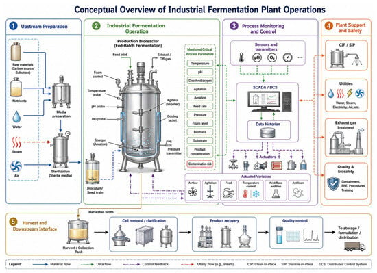
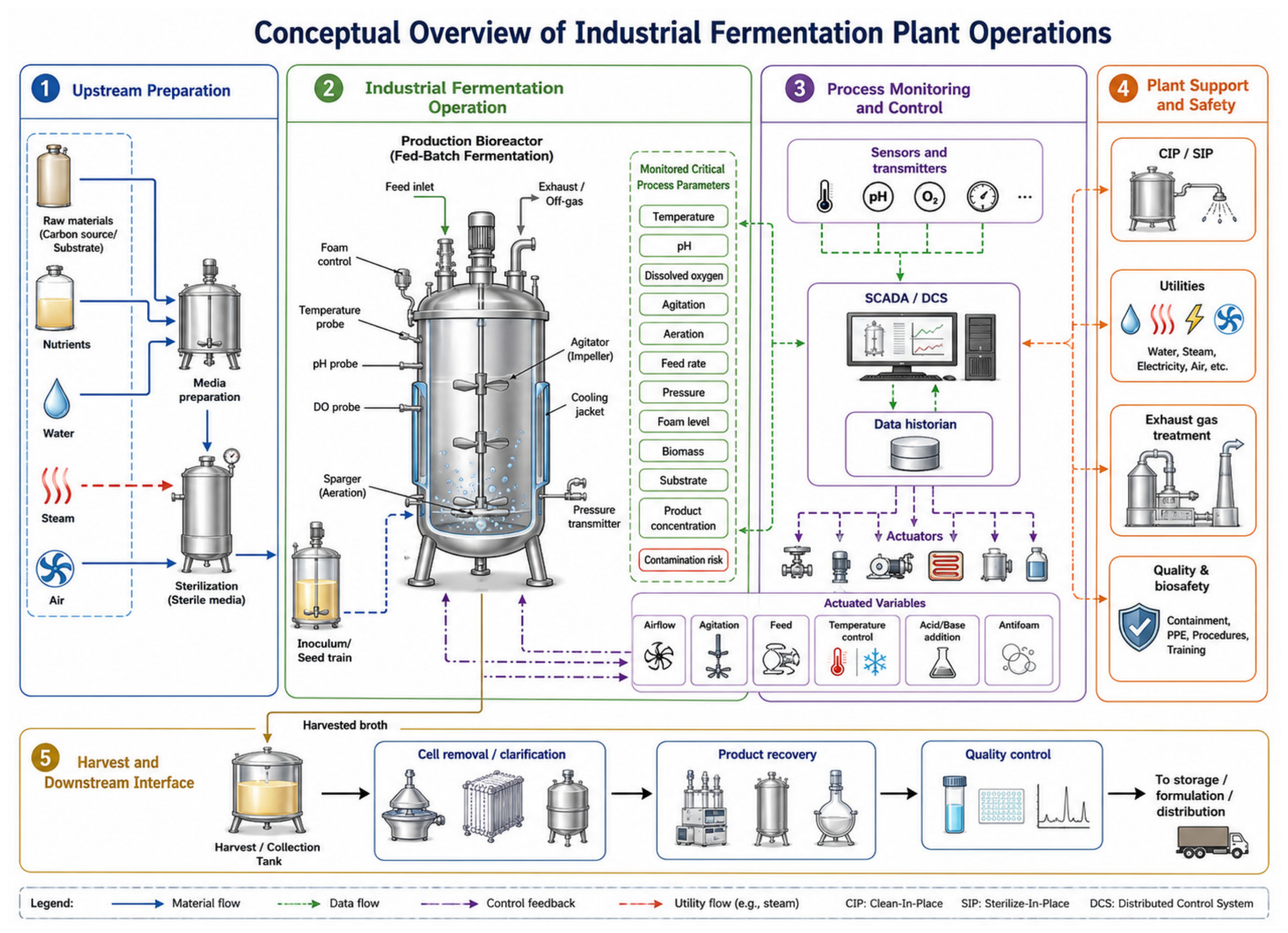
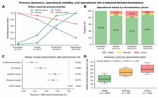
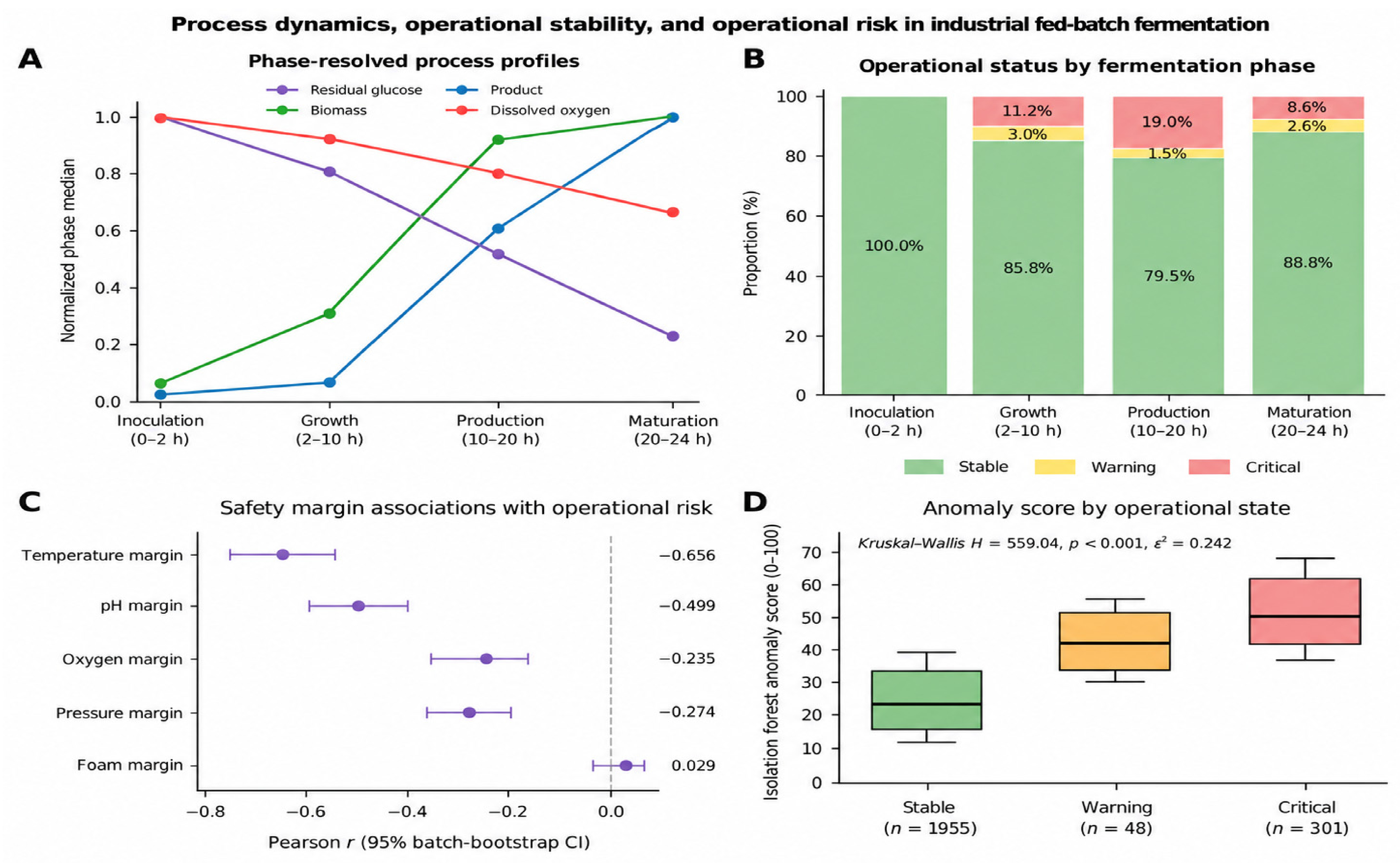
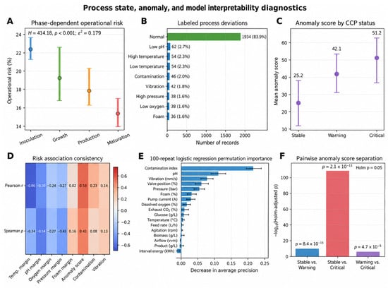
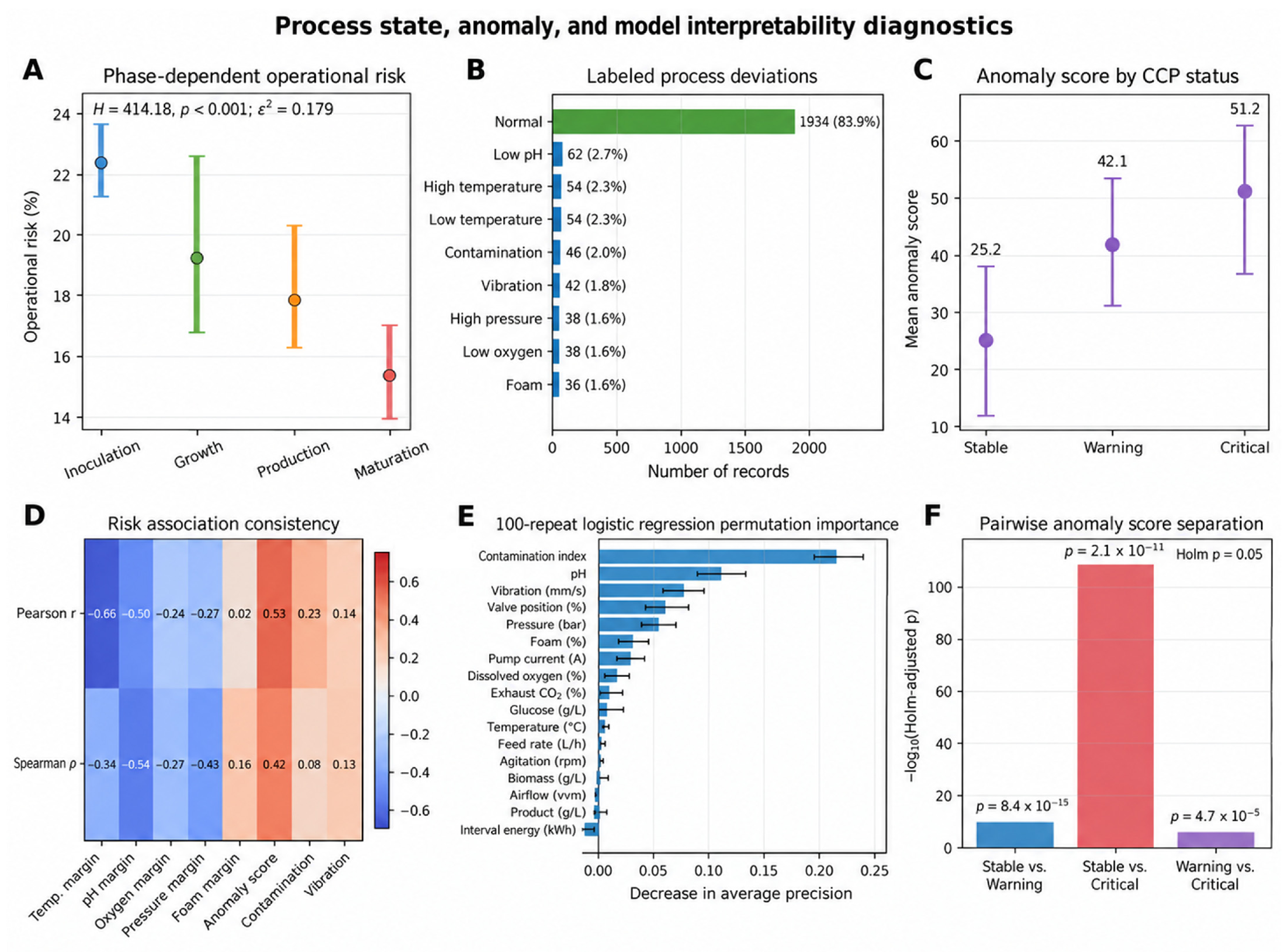
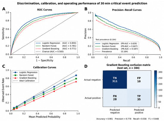
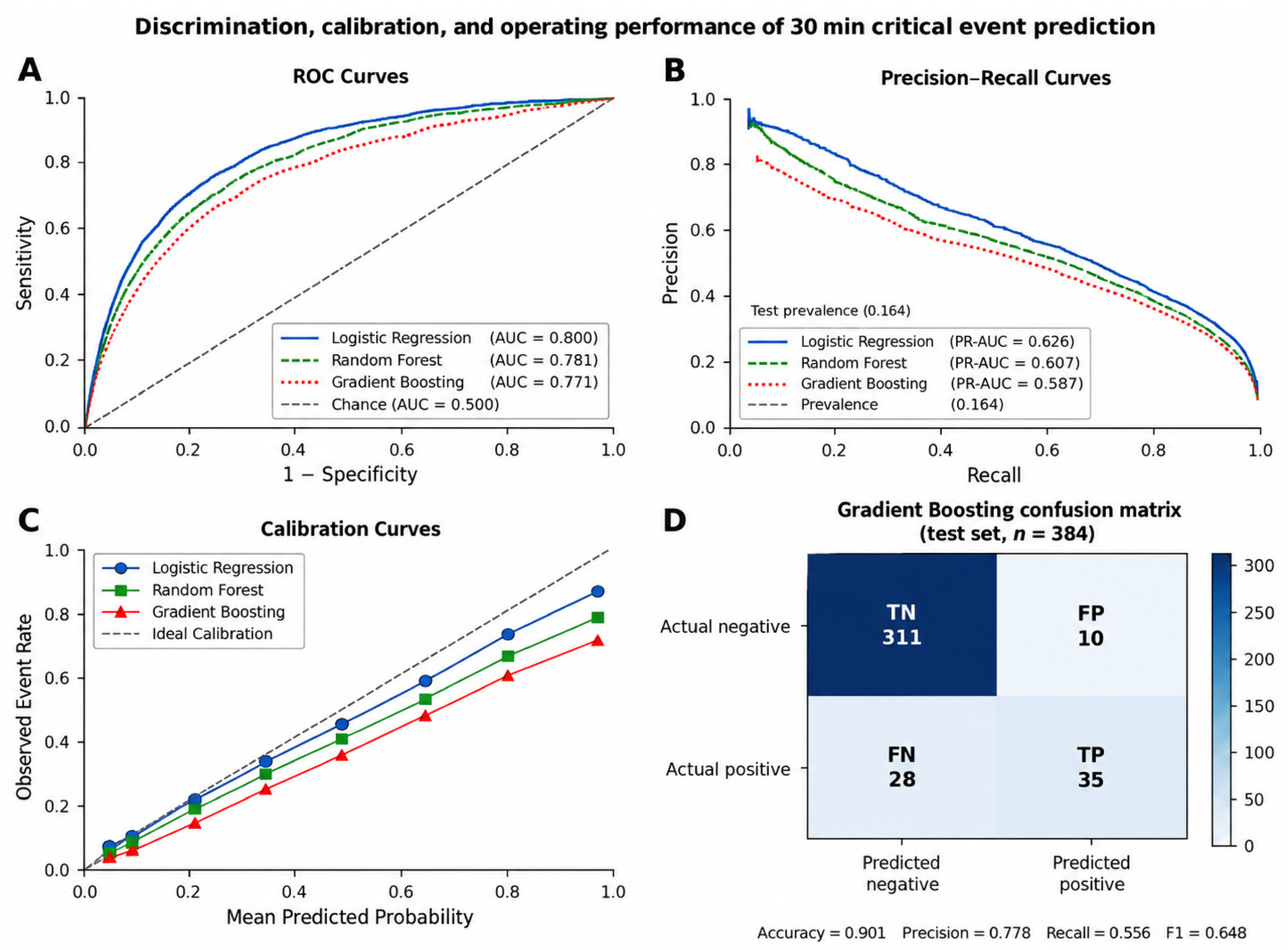
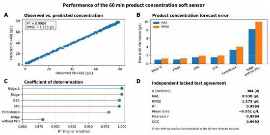
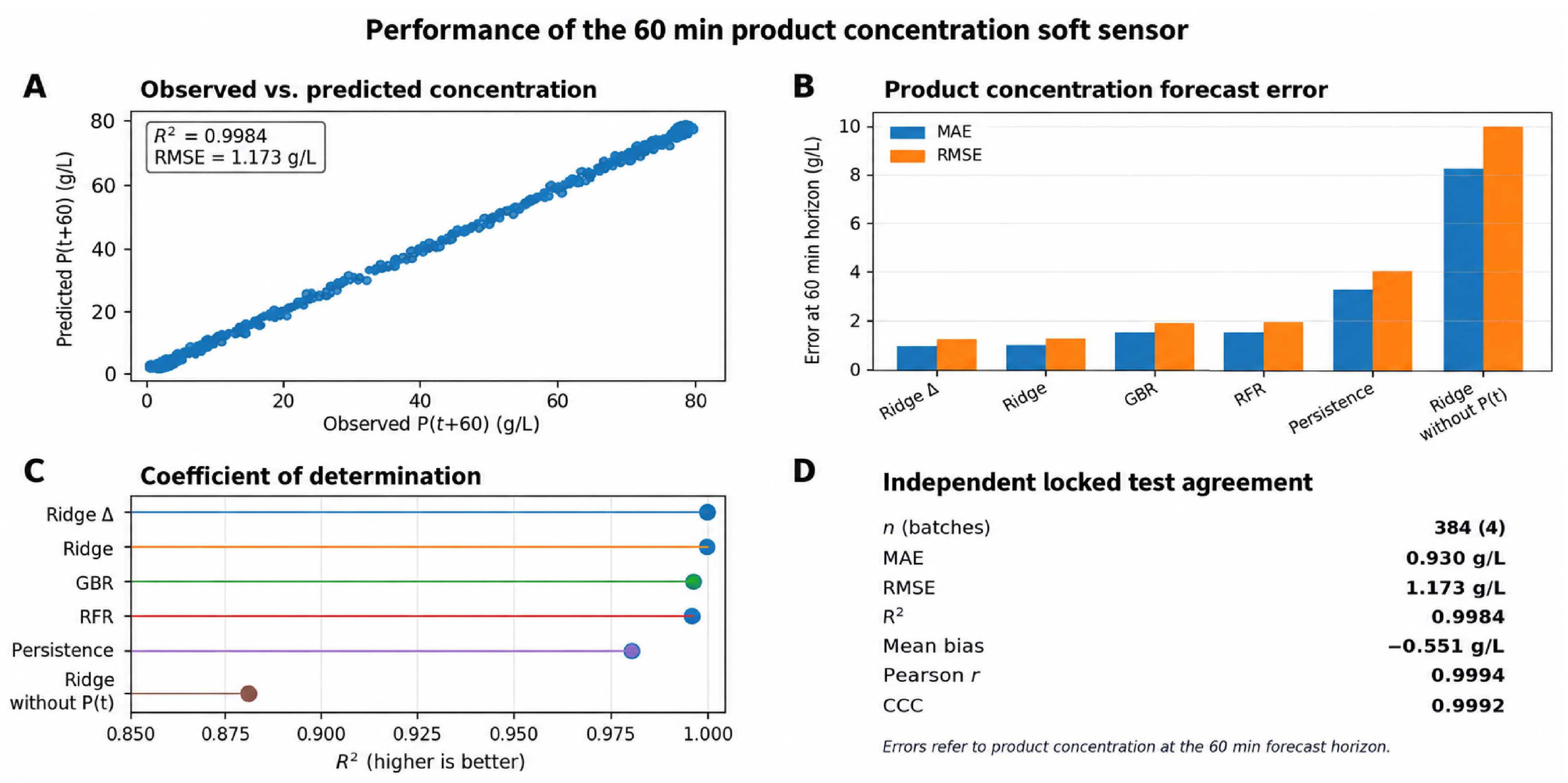
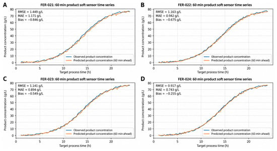
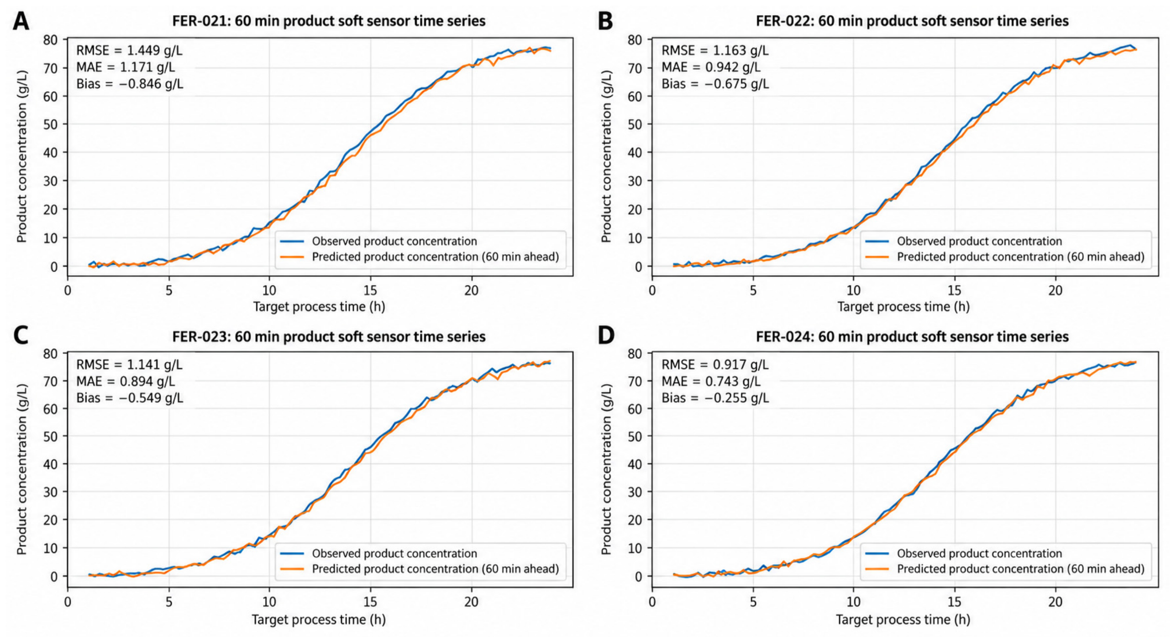
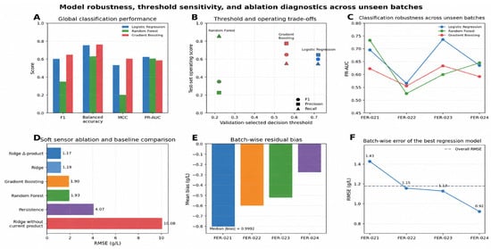
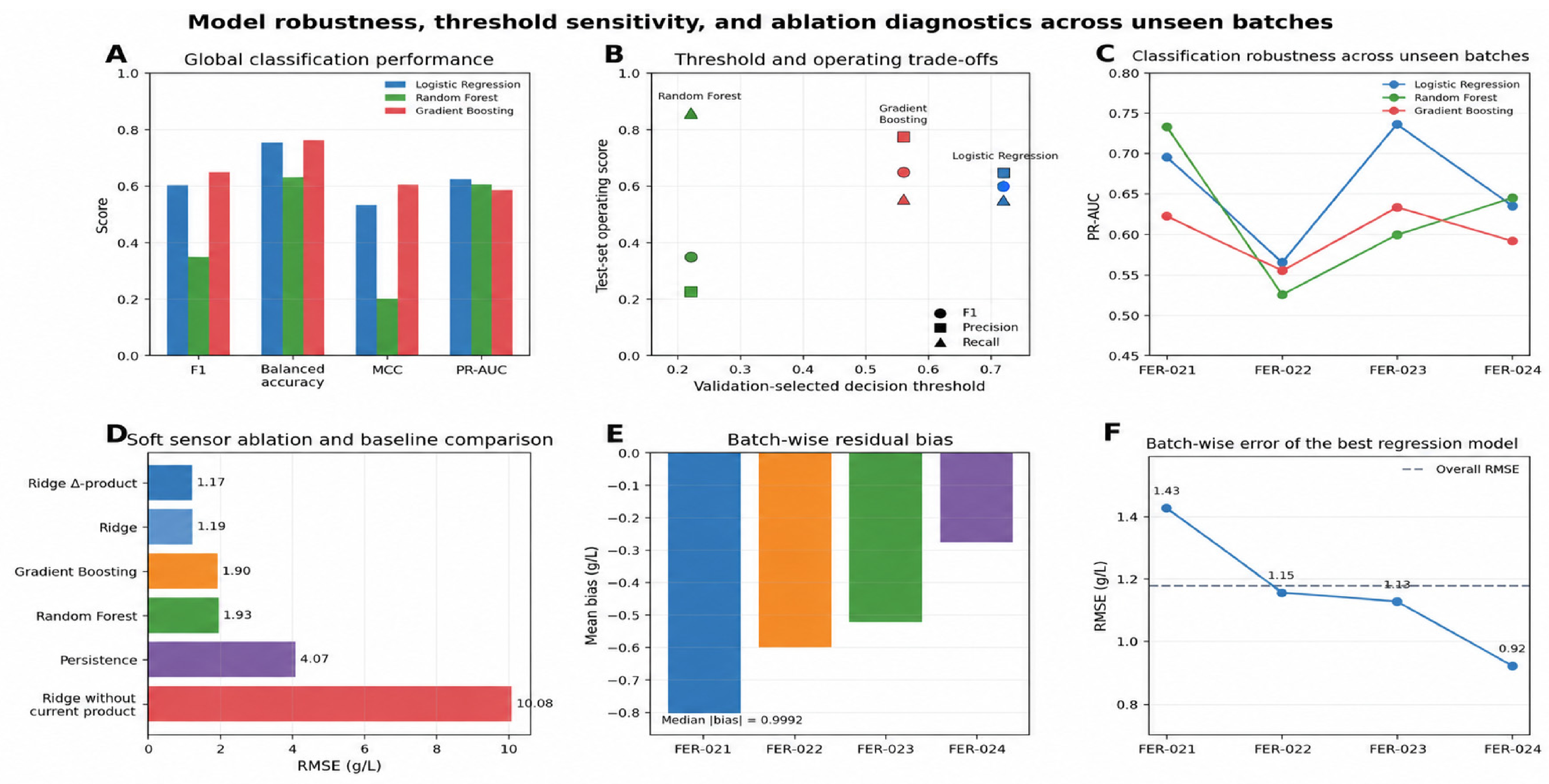
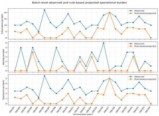
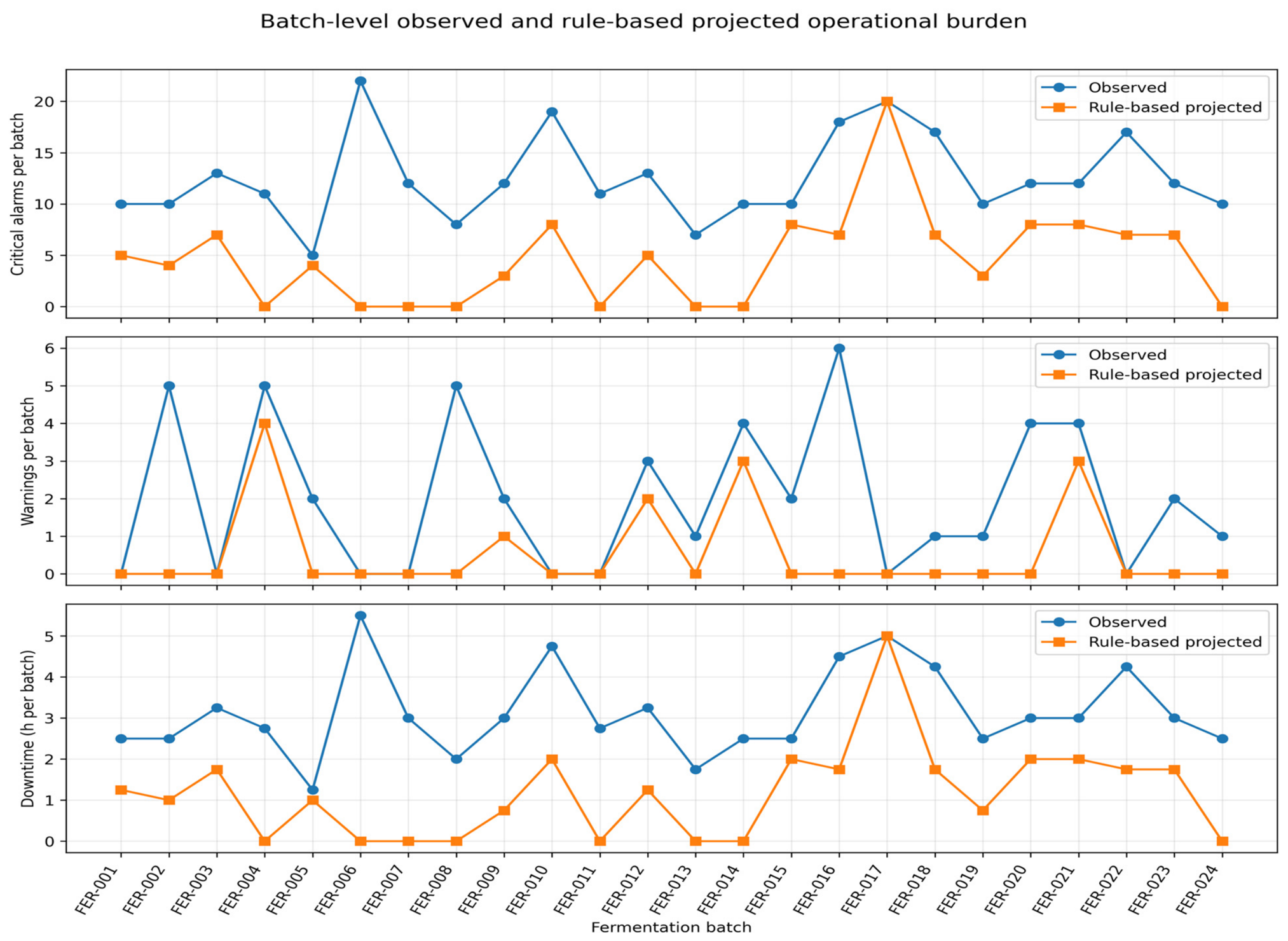

Disclaimer/Publisher’s Note: The statements, opinions and data contained in all publications are solely those of the individual author(s) and contributor(s) and not of MDPI and/or the editor(s). MDPI and/or the editor(s) disclaim responsibility for any injury to people or property resulting from any ideas, methods, instructions or products referred to in the content. |
© 2026 by the authors. Licensee MDPI, Basel, Switzerland. This article is an open access article distributed under the terms and conditions of the Creative Commons Attribution (CC BY) license.