A Multi-Stage Data-Driven Process for Magnetic Azimuth Error Compensation in Horizontal Wells Under Complex Magnetic Environments

Abstract

With the increasing use of horizontal wells in oil and gas development, measurement-while-drilling (MWD) systems require higher magnetic azimuth accuracy to ensure precise trajectory control. This study proposes a three-stage magnetic azimuth error compensation method based on multi-station analysis (MSA). First, the OPTICS clustering algorithm is utilized to identify and remove noise points, and ellipse fitting is applied to suppress radial magnetic interference. Second, an improved MSA model incorporating wellbore trajectory constraints is developed to minimize axial interference and enhance correction stability. Finally, a Gaussian Process Regression (GPR) model, using accelerometer and magnetometer data as features, is introduced to model and compensate for residual nonlinear errors. Experimental validation under simulated complex magnetic conditions shows that OPTICS-based preprocessing significantly improves ellipse fitting and reduces hard magnetic interference. The improved MSA lowers the mean azimuth error to approximately 2.5°, while integrating GPR further decreases it to below 0.04°. The proposed GPR model achieves an R² of 0.99972 and an RMSE of 0.02928° on the test set, confirming its strong nonlinear compensation capability. Overall, the proposed framework effectively suppresses magnetic interference and enhances azimuth accuracy, providing a robust solution for high-precision MWD applications in horizontal wells.

1. Introduction

Horizontal well drilling has become a critical technology for enhancing oil and gas recovery, especially in unconventional reservoir development and old well reconstruction [1,2]. Precise wellbore trajectory control depends on high-accuracy MWD systems, and real-time magnetic azimuth determination is particularly crucial [3,4]. However, horizontal wells suffer from more pronounced magnetic interference compared with vertical or deviated wells. Drill-string magnetization and residual casing magnetization distort magnetometer readings, while near-horizontal wellbore attitudes weaken geomagnetic field projections, making azimuth estimation more sensitive to noise [5]. Moreover, variations in the geomagnetic field can significantly affect drilling efficiency and well placement accuracy, especially in reservoir-scale operations where local magnetic anomalies lead to trajectory deviations and increased positioning uncertainty [6,7,8]. These challenges make conventional magnetic interference correction methods insufficient for the stringent accuracy requirements of horizontal well trajectory control [9].

The key question, therefore, is how to effectively suppress radial and axial magnetic interference while simultaneously modeling nonlinear residual errors in order to achieve robust azimuth estimation under complex downhole environments. This paper addresses the question of how a multi-stage correction framework can be constructed to improve the accuracy and stability of magnetic azimuth determination in horizontal wells.

To address magnetic interference, various approaches have been explored. For radial correction, Li et al. applied DBSCAN to remove noise points and enhance ellipse fitting reliability [10], while Miu et al. incorporated OPTICS into compass ellipse fitting, reducing parameter sensitivity and improving accuracy [11]. For axial interference, Bulychenkov proposed an MSA-based correction method that constrains interference values using trajectory functions, thereby improving stability and applicability [12]. Although these methods improve interference suppression, they still fall short of fully capturing nonlinear error patterns in complex downhole conditions, limiting the accuracy of azimuth estimation.

Beyond these traditional methods, researchers have also investigated hardware-based and data-driven strategies. On the hardware side, integrating magnetometers with gyroscopes and accelerometers through sensor fusion and Kalman filtering has been shown to mitigate magnetic distortions [13,14]. However, such solutions often increase system complexity and cost, limiting their use in drilling tools. On the data-driven side, machine learning methods such as artificial neural networks (ANNs) and support vector machines (SVMs) have been applied to magnetometer calibration and error compensation [15,16]. While these approaches show promise, their effectiveness tends to rely heavily on large training datasets and careful parameter tuning, which constrains their robustness under highly variable downhole environments.

Among the various learning-based techniques, GPR has attracted particular attention because of its ability to model nonlinear mappings while providing principled uncertainty quantification. GPR has been widely adopted in magnetic field modeling and interference compensation. For example, Solin et al. employed GPR with physical prior constraints to interpolate and reconstruct environmental magnetic fields [17]; Kuevor et al. applied GPR to UAV navigation and indoor positioning, achieving improved attitude estimation under interference [18]; and Edridge and Kok developed a noisy-input GPR formulation to enhance robustness in magnetic field interpolation [19]. These studies demonstrate that GPR offers clear advantages for modeling environment-dependent nonlinear disturbances, making it a promising tool for magnetic azimuth correction in horizontal wells.

Motivated by the limitations of existing approaches and the strengths of GPR, this paper proposes a multi-stage correction framework that integrates clustering-based denoising, constrained optimization, and nonlinear error compensation. The main contributions of this work are summarized as follows:

• For the first time, OPTICS clustering is combined with ellipse fitting to suppress radial magnetic interference, enabling adaptive noise point identification and improved ellipse fitting accuracy, which significantly enhances azimuth reliability in complex downhole environments;
• A constrained optimization model based on MSA is proposed for axial interference correction, where wellbore trajectory constraints are introduced to mitigate cross-coupling effects, yielding notable improvements in both correction stability and applicability compared with conventional MSA approaches;
• GPR is incorporated to model and compensate for residual nonlinear errors, where multidimensional features from accelerometers and magnetometers enable fine-grained characterization of error distributions, thereby enhancing robustness and significantly improving the overall accuracy of magnetic azimuth determination in horizontal wells.

The remainder of this paper is organized as follows. Section 2 introduces the theoretical background of multi-station analysis and details the proposed three-stage error correction framework, including OPTICS-based denoising, ellipse fitting, and GPR modeling. Section 3 describes the experimental setup and provides a comprehensive analysis of the results under different azimuth conditions. Section 4 summarizes the findings, highlights the advantages of the proposed approach compared with conventional methods, and discusses its engineering implications for high-precision trajectory control in horizontal wells.

2. Methods

This section describes the design and implementation of the proposed multi-stage magnetic orientation error compensation method. First, the attitude measurement principle of the measurement while drilling system and the basic theoretical framework of the multi-point analysis method are explained, laying the foundation for subsequent methods. Second, a least-squares ellipse fitting method is introduced in the radial plane, combined with the OPTICS clustering algorithm to denoise and correct the raw data. Finally, based on the improved multi-point analysis results, a GPR model is constructed to model and compensate for residual nonlinear errors. Each of these methods will be introduced and analyzed one by one to form a complete error compensation process.

2.1. Multi-Station Attitude Measurement Principle

2.1.1. Attitude Measurement Principle

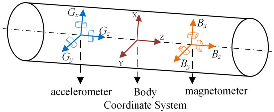
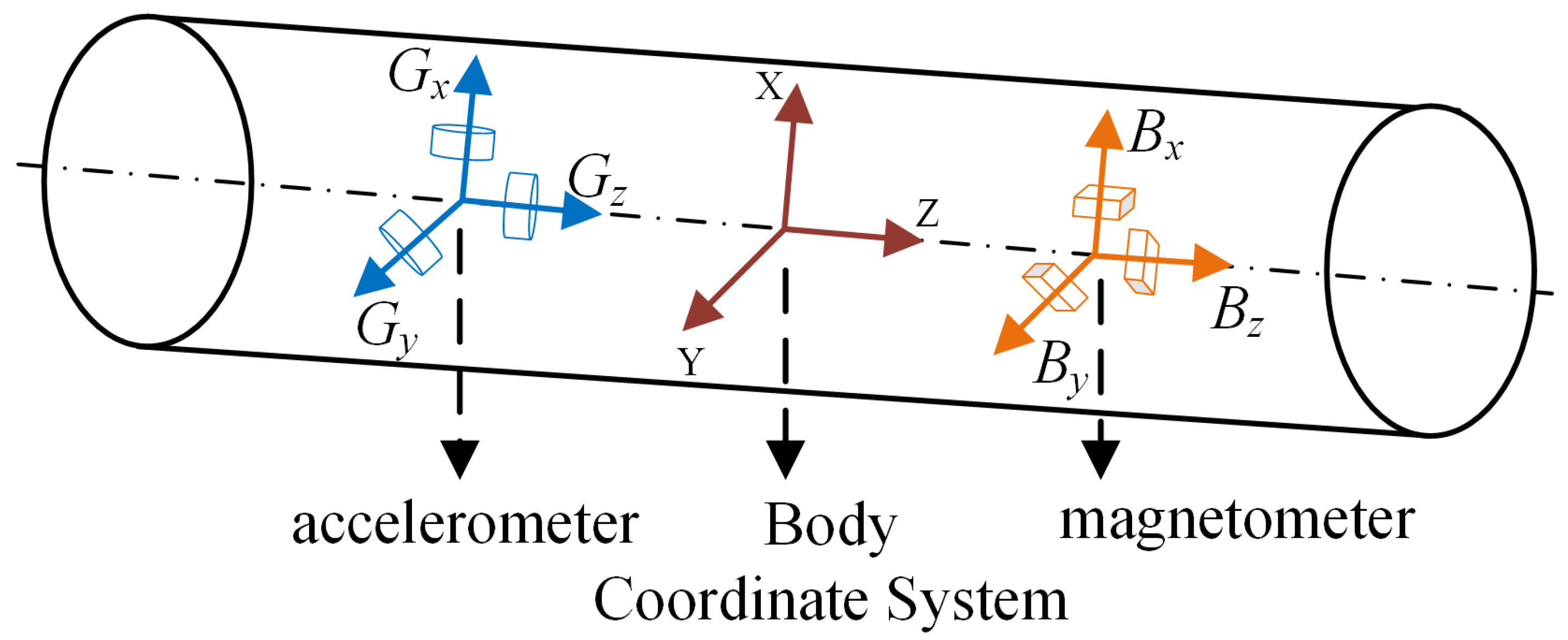
In the MWD system, three-axis accelerometers and magnetometers are installed along the three orthogonal coordinate axes of the carrier coordinate system to form a basic MWD system [20]. As shown in Figure 1, the accelerometer and magnetometer are used to measure the gravity field and geomagnetic field components in the three coordinate axis directions to calculate the real-time attitude of the tool [21].

Figure 1. Schematic diagram of the inclinometer while drilling.

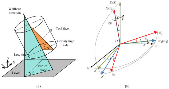
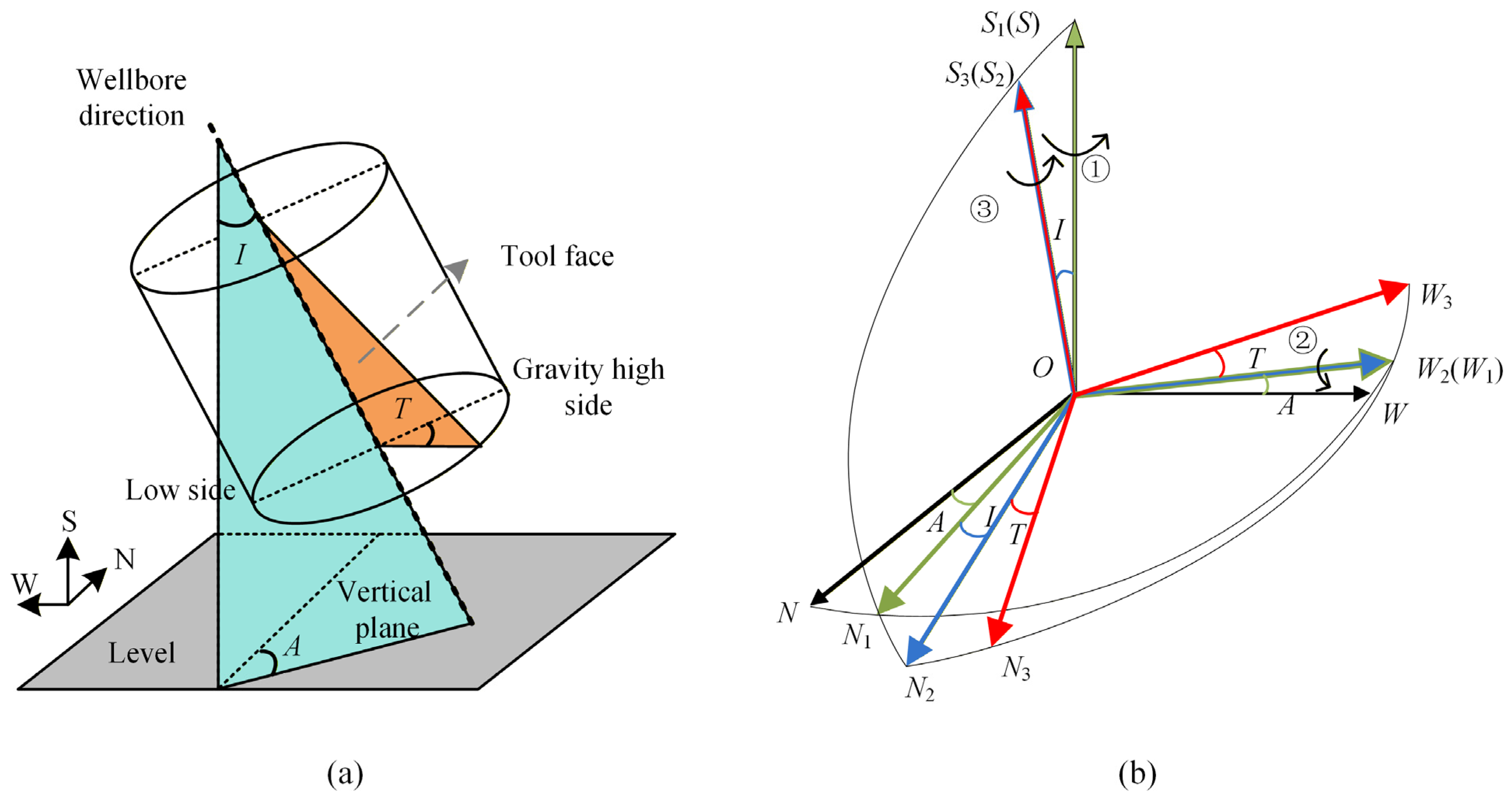
The attitude of the downhole tool is composed of three parameters, namely the inclination angle (I), the azimuth angle (A) and the tool face angle (T). The attitude measurement system is shown in Figure 2a. The attitude calculation algorithm often involves the conversion between the carrier coordinate system and the inertial coordinate system [22]. Downhole drilling attitude measurement predominantly employs the geographic north-west-sky (O-NWS) coordinate system. The carrier coordinate system is rotated to the inertial coordinate system via Z-Y-Z coordinate system rotation [23], as illustrated in Figure 2b. The rotation matrix of three rotations is recorded as R_A, R_I and R_T respectively, and the rotation matrix R of the whole coordinate system transformation can be obtained as follows:

$$R=R_A{R}_I{R}_T$$

(1)

Figure 2. Principle of attitude measurement in wellbore: (a) definition of inclination, azimuth, and tool face angle; (b) coordinate system transformation.

As shown in Figure 2, the relationship between the carrier coordinate system O-NWS and the inertial coordinate system O-N₃W₃S₃ can be expressed as:

$$\left[\begin{array}{l}N\\ W\\ S\end{array}\right]=R\cdot \left[\begin{array}{l}{N}_3\\ W_3\\ S_3\end{array}\right]$$

(2)

During the rotation of the coordinate system, the corresponding changes of the accelerometer and magnetometer are given as:

$$\left[\begin{array}{l}{G}_x B_x\\ G_y B_y\\ G_z B_z\end{array}\right]=R\cdot \left[\begin{array}{l}0 B_N\\ 0 B_W\\ -G B_S\end{array}\right]$$

(3)

where Gx, Gy, and Gz represent the three-axis components of the measured accelerometer signal; G is the actual gravity acceleration; Bx, By, and Bz and B_N, B_W, and B_S represent the three-axis components of the measured fluxgate signal and the components of the geomagnetic field in the geographic north, west, and sky directions, respectively.

According to the projection relationship between the gravity field and the magnetic field in the carrier coordinate system, the right-handed coordinate system is used to perform Euler rotation to obtain the solution relationship between the measurement value of the three-axis sensor and the azimuth angle [24]:

$$\left\{\begin{array}{ll}I& =\arccos (G_z/\sqrt{G_x^2+G_y^2+G_z^2})=\\ & \arcsin (\sqrt{{(G_x)}^2+{(G_y)}^2}/\sqrt{G_x^2+G_y^2+G_z^2})\\ T& =-\arctan (G_y/G_x)=-\sin (G_x/g\sin I)=\\ & \pi -\arcsin (G_y/\sin I)\\ A& =\arctan (-B_x\cdot \sin T+B_y\cdot \cos T/\\ & \cos I(B_x\cos T+B_y\sin T)-B_z\sin I)\end{array}\right.$$

(4)

2.1.2. The Basic Principle of MSA

Brooks proposed MSA method, which simultaneously processes magnetic field data from multiple measurement points, uses the attitude differences between different measurement points, and establishes a set of equations to solve sensor error parameters, thereby performing magnetic interference correction [25]. Compared to the traditional single-point calibration method, MSA does not rely on an external reference magnetic field. It uses the measurement values of multiple measurement points to infer the sensor error by minimizing the total magnetic field variance (the deviation between the measured value and the reference value) [26]. The formulas are as follows:

$$\left\{\begin{array}{l}{B}_{x\mathrm{corri}}=B_{x\mathrm{measi}}-{\epsilon }_x\\ B_{y\mathrm{corri}}=B_{y\mathrm{measi}}-{\epsilon }_y\\ B_{z\mathrm{corri}}=B_{z\mathrm{measi}}-{\epsilon }_z\end{array}\right.$$

(5)

$$B_{\mathrm{vref}}={\displaystyle \frac{1}{N}}{\displaystyle \sum _{i=1}^N{B}_{\mathrm{vi}}}$$

(6)

$$B_{\mathrm{nref}}={\displaystyle \frac{1}{N}}{\displaystyle \sum _{i=1}^N{B}_{\mathrm{ni}}}$$

(7)

$$B_{\mathrm{vi}}={\displaystyle \frac{B_{x\mathrm{corri}}{G}_{xi}+B_{y\mathrm{corri}}{G}_{yi}+B_{z\mathrm{corri}}{G}_{zi}}{\sqrt{G_{xi}^2+G_{yi}^2+G_{zi}^2}}}$$

(8)

$$B_{\mathrm{hi}}=\sqrt{B_{x\mathrm{corri}}^2+B_{y\mathrm{corri}}^2+B_{z\mathrm{corri}}^2-B_{\mathit{vi}}^2}$$

(9)

$$V={\displaystyle \sum _{i=1}^N[{(B_{\mathrm{hi}}-B_{\mathrm{href}})}^2+}{(B_{\mathrm{vi}}-B_{\mathrm{vref}})}^2)]/(N-1)$$

(10)

where B_xmeasi, B_ymeasi, and B_zmeasi are the magnetic field signal components of the magnetometer at the i-th measuring station. B_xcorri, B_ycorri, and B_zcorri are the magnetic field values of the magnetometer after three-axis correction. G_xi, G_yi, and G_zi are the components of the accelerometer at the i-th measuring station. B_hi and B_vi are the vertical and horizontal magnetic field components of the Earth’s magnetic field, respectively. B_href is the reference value of the vertical component for all measuring stations. B_vref is the reference value of the horizontal component for all measuring stations. ε_x, ε_y, and ε_z are the interfering magnetic field values along the x, y, and z axes.

The X-axis and Y-axis data of the magnetic sensor are corrected by ellipse fitting, and the Z-axis data are further corrected using the single-axis MSA method (hereafter referred to as the improved MSA method). Compared with the traditional MSA method, the single-axis MSA method reduces cross-coupling errors caused by sensor inconsistencies, lowers data dimensionality, and facilitates fast processing. The optimization objective of the improved MSA method is defined as follows:

$$B_{\mathrm{vi}}={\displaystyle \frac{B_{x\mathrm{radial}}{G}_{xi}+B_{y\mathrm{radial}}{G}_{yi}+B_{z\mathrm{corri}}{G}_{zi}}{\sqrt{G_{xi}^2+G_{yi}^2+G_{zi}^2}}}$$

(11)

$$B_{\mathrm{hi}}=\sqrt{B_{x\mathrm{radial}}^2+B_{y\mathrm{radial}}^2+B_{z\mathrm{corri}}^2-B_{\mathrm{vi}}^2}$$

(12)

$$V={\displaystyle \sum _{i=1}^N[{(B_{\mathrm{hi}}-B_{\mathrm{href}})}^2+}{(B_{\mathrm{vi}}-B_{\mathrm{vref}})}^2)]/(N-1)$$

(13)

Here, B_xradial and B_yradial represent the magnetic field components in the X- and Y-directions after radial correction, which are obtained from the ellipse fitting process.

2.2. Improved MSA Method

2.2.1. Ellipse Fitting Using the Least Squares Method

When there is no external magnetic interference and the instrument rotates at high speed for one circle, the drilling depth can be ignored, and the two radial components of the magnetic field B_x and B_y are output as a circle [27]. However, due to the non-orthogonality error, sensitivity error and zero error of the magnetic sensor, as well as the interference of the surrounding magnetic field, the actual output will be close to an ellipse rather than a standard circle [28]. Therefore, the radial error correction of the magnetic sensor can be achieved by obtaining its standard parameter equation through ellipse fitting.

The ellipse can be expressed by a general quadratic polynomial, as shown in Formula (13):

$$F(k,x)=a\cdot x^2+b\cdot x\cdot y+c\cdot y^2+d\cdot x+e\cdot y+\mathbf{f}$$

(14)

where k = [a b c d e f]^T is the parameter vector. D (k,x_i) is the distance from point (x_i,y_i) to the curve F (k,x) = 0. The ellipse fitting problem is actually to find a set of parameter vectors that minimizes the sum of the squares of the distances from all experimental data to the curve F (k,x) = 0, that is:

$$\underset{k}{\min }{\displaystyle \sum _{i=1}^{n}D{(\mathit{k},{\mathit{x}}_i)}^2}$$

(15)

The corrected radial magnetic field intensity can be obtained by passing the elliptic parameters through Equations (16) and (17).

$$\theta =\mathrm{arccot}((a-c)/b)$$

(16)

$$\left[\begin{array}{l}{B}_{x\mathrm{corri}}\\ B_{y\mathrm{corri}}\end{array}\right]=\left[\begin{array}{l}\cos \theta \sin \theta \\ -\sin \theta \cos \theta \end{array}\right]\left[\begin{array}{l}{B}_{x\mathrm{measi}}\\ B_{y\mathrm{measi}}\end{array}\right]$$

(17)

2.2.2. OPTICS Clustering Algorithm

Although the ellipse fitting algorithm based on the minimum algebraic distance is simple to implement and has high computational efficiency, the fitting accuracy decreases significantly, and the recognition rate is low when noise exists. Therefore, the original data needs to be denoised before using the ellipse fitting algorithm [29]. The OPTICS algorithm starts from a random object point and expands towards the area with the densest data, generating an ordered sequence containing reachable distance information for all object points, effectively solving the parameter sensitivity problem of the traditional density clustering algorithm DBSCAN [30].

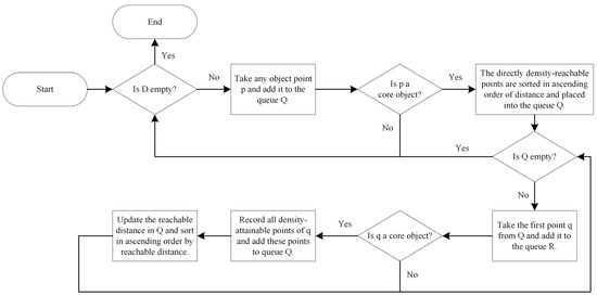
In the clustering process, if the number of points in the domain of object point p is not less than the set MinPts, then p is called a core object, and the minimum domain radius ε required for it to become a core object is defined as its core distance. For an object point m and a core point p, if the distance from point m to point p is greater than the core distance of point p, then the reachable distance of point m is the actual distance between point p and point m. Otherwise, the reachable distance of point m is the core distance of point p. If an object point q is within the domain of the core object p, then point q is a directly density-reachable object of point p. The ordered queue stores the core objects and their directly density-reachable objects in ascending order of reachable distance, and the result queue is used to record the final data output order [31]. D represents the dataset, Q represents the ordered sequence, and R represents the result sequence. The OPTICS algorithm flow is shown in Figure 3.

Figure 3. OPTICS algorithm flow chart.

Firstly, the OPTICS clustering algorithm is employed to preprocess the raw data by identifying and eliminating noise points, followed by ellipse fitting. This procedure effectively guarantees the accuracy of the ellipse fitting and mitigates radial magnetic interference errors.

2.2.3. Gaussian Process Regression

Due to interference from multiple factors, the error distribution of magnetic fields is often difficult to model. Magnetic field data are usually continuous in space and have a certain correlation. GPR is very suitable for compensating for such spatially continuous errors. It is a non-parametric Bayesian method that expresses the correlation between different input points using a covariance function [32]. If x is an m-dimensional parameter with x∈R^m, the corresponding Gaussian process is denoted as {f(x), x∈R^m}. Its properties are determined by the mean function μ(x) and the covariance function k(x_i, x_j). If the joint distribution is Gaussian, then the resulting stochastic process is referred to as a Gaussian process, which is defined as follows [33]:

$$\mu (\mathit{x})=E\left[f(\mathit{x})\right]$$

(18)

$$k(x_i,x_j)=E\left[(f(x_i)-\mu (x_i))\times \right.\left.(f(x_j)-\mu (x_j))\right]$$

(19)

$$f(x)\sim GP\left[\mu (x),k(x_i,x_j)\right]$$

(20)

If the Gaussian white noise n with a mean of 0 and a variance of σ_n² is taken into account in the observed target value y, a Gaussian process regression model can be established [34], which is defined as follows:

$$\left\{\begin{array}{l}y=f(x)+n\\ n\sim N(0,{\sigma }_n^2{I}_n)\end{array}\right.$$

(21)

Since f(x) follows a Gaussian distribution, y also follows a Gaussian distribution. Therefore, the collection of all observed target values y in the sample set forms a new Gaussian process, which can be expressed as:

$$y\sim GP(\mu (x),k(x_i,x_j)+{\sigma }_N^2{\delta }_{i,j})$$

(22)

In the formula, δ is the Kronecker delta function, where δ_i,j = 1 if i = j, and δ_i,j = 0 otherwise.

If the observed data samples are divided into a training set R = {x_i, x_j} and a test set T = {x_i, x_j}, the prior probability distribution of the training set is given as [35]:

$$y_R\sim N(\mu (X_R)),K(X_R,X_R)+{\sigma }_n^2{I}_n)$$

(23)

The test set also follows a Gaussian distribution, and the outputs of the training set y_R together with the outputs of the test set y_T constitute the prior of the joint probability distribution:

$$\begin{array}{c}\left[\begin{array}{l}{y}_R\\ y_T\end{array}\right]\sim \left(\left[\begin{array}{l}\mu (X_R)\\ \mu (X_T)\end{array}\right]\right.,\\ \left.\left[\begin{array}{l}K(X_R,X_R)+{\sigma }_{R,n}^2{I}_n K(X_R,X_T)\\ K(X_T,X_R) K(X_T,X_T)\end{array}\right]\right)\end{array}$$

(24)

where K(X_R, X_R) and K(X_T, X_T) are symmetric positive-definite covariance matrices of the training set and the test set, respectively. The matrix elements k_ij = k(x_i, x_j) measure the correlation between inputs x_i and x_j. K(X_T, X_R) = K(X_R, X_T)^T denotes the covariance matrix between the training set R and the test set T, and I_n is the identity matrix. According to Bayes’ theorem, given the training samples and the test inputs, the posterior distribution of the test set can be inferred as:

$$y_T|X_R,y_R,X_T\sim N(\stackrel{-}{y_T},\mathrm{cov}(y_T))$$

(25)

where ȳ_T is the mean of the test set outputs, and cov(y_T) is the variance of the test set, which are given as follows:

$$\begin{array}{l}\overline{y_T}=K(X_T,X_R)\times {\left[K(X_R,X_R)+{\sigma }_n^2{I}_n\right]}^{-1}{y}_R\\ \mathrm{cov}(y_T)=K(X_T,X_T)-K(X_T,X_R)\times {\left[K(X_R,X_R)+{\sigma }_n^2{I}_n\right]}^{-1}K(X_R,X_T)\end{array}$$

(26)

During the prediction process of the GPR model, an appropriate kernel function can be selected based on sample attributes to transform nonlinear relationships between data points into linear ones. This simplifies the solution of nonlinear problems by solving prior problems [36]. The Automatic Relevance Determination kernel (ARD) incorporates an automatic relevance assessment mechanism, assigning an independent length scale to each input feature. This enables effective identification and suppression of redundant features with minimal predictive impact, thereby enhancing the model’s generalization capability and prediction accuracy [37]. In contrast, the Matern kernel is more suitable for non-smooth or high-noise data. The standard Gaussian kernel assumes equal importance for all features, which may limit its modeling capability in high-dimensional or unevenly contributing scenarios [38]. Therefore, the use of the ARD kernel in this method is more conducive to fully extracting the feature information of each input variable, thereby achieving more precise error modeling and compensation. The ARD kernel is formulated as:

$$K(x_i,x_j)={\sigma }_f^2\times \exp (-{\displaystyle \frac{1}{2}}{\displaystyle \sum _{d=1}^D\frac{{(x_{i,d}-x_{j,d})}^2}{(l_d^2)}})$$

(27)

where x_i and x_j are the i-th and j-th samples in the input space, D denotes the dimension of the input features, $l_d^2$ represents the length scale of the d-th input feature, and ${\sigma }_f^2$ is the output variance of the kernel function.

The root mean square error (RMSE), mean absolute error (MAE), and coefficient of determination (R²) are used to evaluate the model performance, and are defined as follows:

$$\mathrm{RMSE}=\sqrt{{\displaystyle \frac{1}{N}}{\displaystyle \sum _1^N{(A_i-\stackrel{\wedge }{A_i})}^2}}$$

(28)

$$\mathrm{MAE}={\displaystyle \frac{1}{n}}{\displaystyle \sum _{i=1}^N|A_i-\stackrel{\wedge }{A_i}|}$$

(29)

$${\mathrm{R}}^2=1-{\displaystyle \frac{{\displaystyle {\sum }_{i=1}^N(A_i-{\stackrel{\wedge }{A}}_i)}}{{\displaystyle {\sum }_{i=1}^N(A_i-{\stackrel{-}{A}}_i)}}}$$

(30)

where A_i is the experimental ideal azimuth, Â is the compensated azimuth, and Ā_i is the mean of the experimental ideal azimuth.

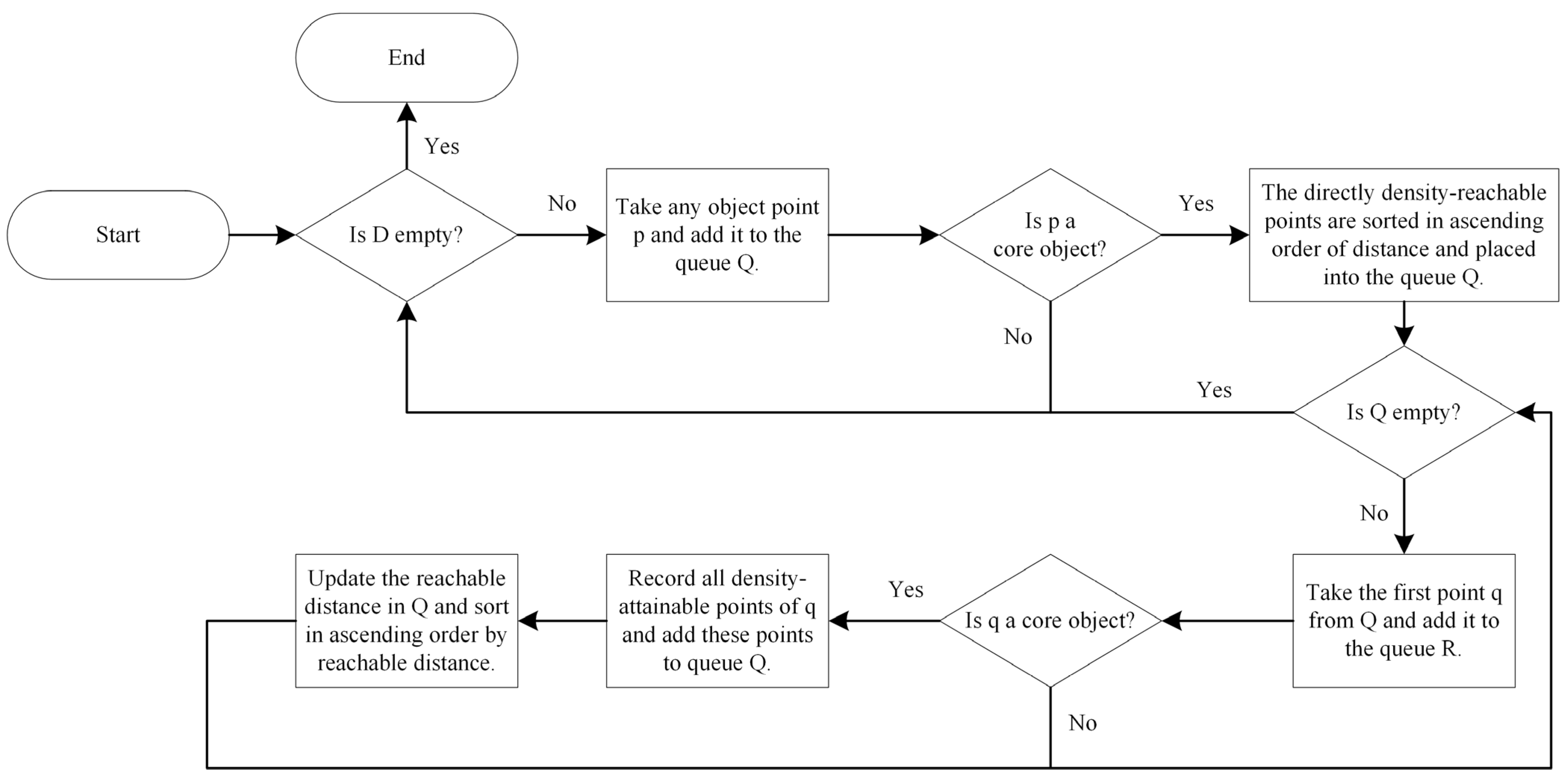
Using the triaxial measurement data from accelerometers and magnetometers as input, and the residuals from the improved MSA method as model data, a Gaussian Process Regression (GPR) model was constructed to compensate for the remaining nonlinear errors. The overall workflow of the multi-station magnetic azimuth error correction based on Gaussian process fusion is illustrated in Figure 4. All model training and computations in this study were performed on a desktop computer equipped with a 12th Generation Intel Core i5-12490F CPU (6 cores and 12 threads, base frequency 3.00 GHz), 16 GB of RAM, and a 64-bit Windows operating system.

Figure 4. Algorithm flowchart.

3. Results and Discussion

3.1. Experimental Setup

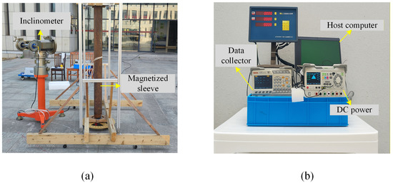
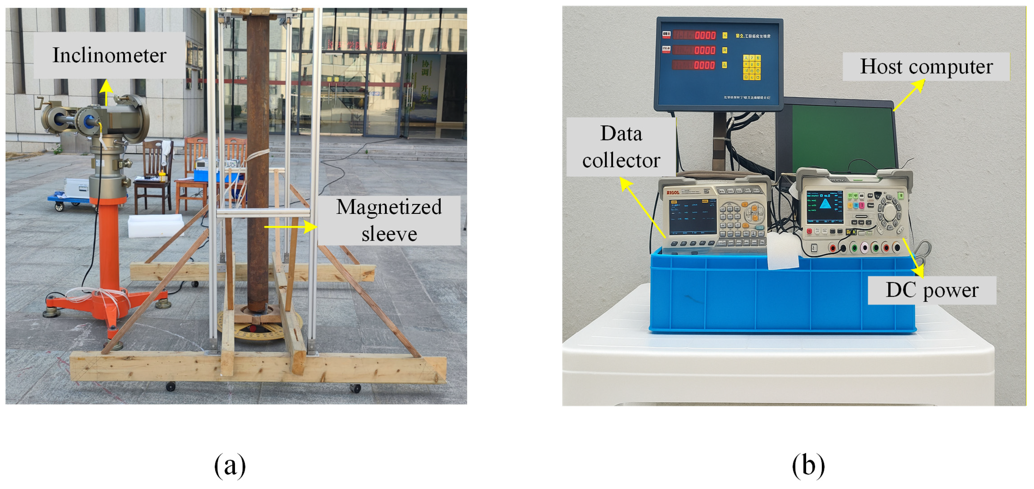
The experimental device mainly includes a DX-4C inclinometer directional sensor, a 3 m long and 150 mm diameter magnetized casing, an aluminum alloy casing bracket and a wooden placement rack, a digital collector, and a power supply. The experiment introduced a magnetized casing to simulate the complex magnetic field conditions faced by actual downhole magnetic sensors, thereby verifying the attitude measurement and error correction capabilities of the proposed MSA method fused with the Gaussian process under magnetic interference conditions.

The distance between the magnetized casing and the inclinometer sensor axis is referred to as the relative distance, which was fixed at 1 m, while the well inclination was maintained at 90°. The angle between the line connecting the magnetic casing and the inclinometer sensor axis and the magnetic north is defined as the relative azimuth. Eight azimuths of 30, 60, 120, 150, 210, 240, 300, and 330° are selected for experimental measurements. The tool face angle started from 0° and rotated at 5° intervals up to 360°. Each measuring point was repeatedly sampled eight times to obtain the average value. The experimental setup is illustrated in Figure 5.

Figure 5. Experimental setup: (a) experimental environment setting; (b) experimental instruments and equipment.

After a single uniform magnetization, the internal magnetic flux density of the steel casing was approximately 3 mT. No subsequent magnetization or demagnetization was performed during the experiments. Because the magnetometer was positioned at different azimuthal angles around the casing, the measured magnetic field components varied with direction, which reflects the spatial characteristics of the magnetic dipole field rather than any change in the magnetization strength of the casing.

3.2. Experimental Results Analysis

3.2.1. OPTICS Denoising and Ellipse Fitting

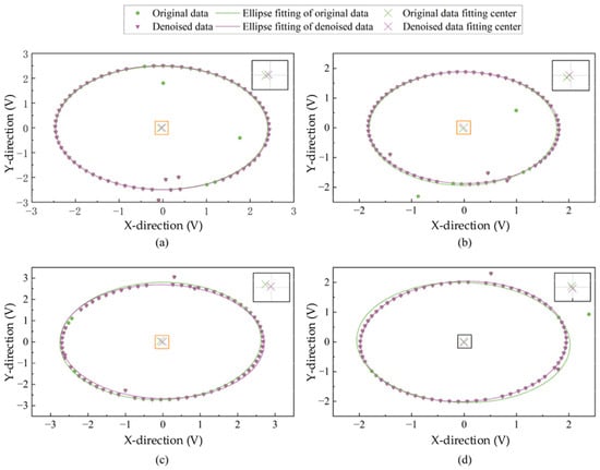
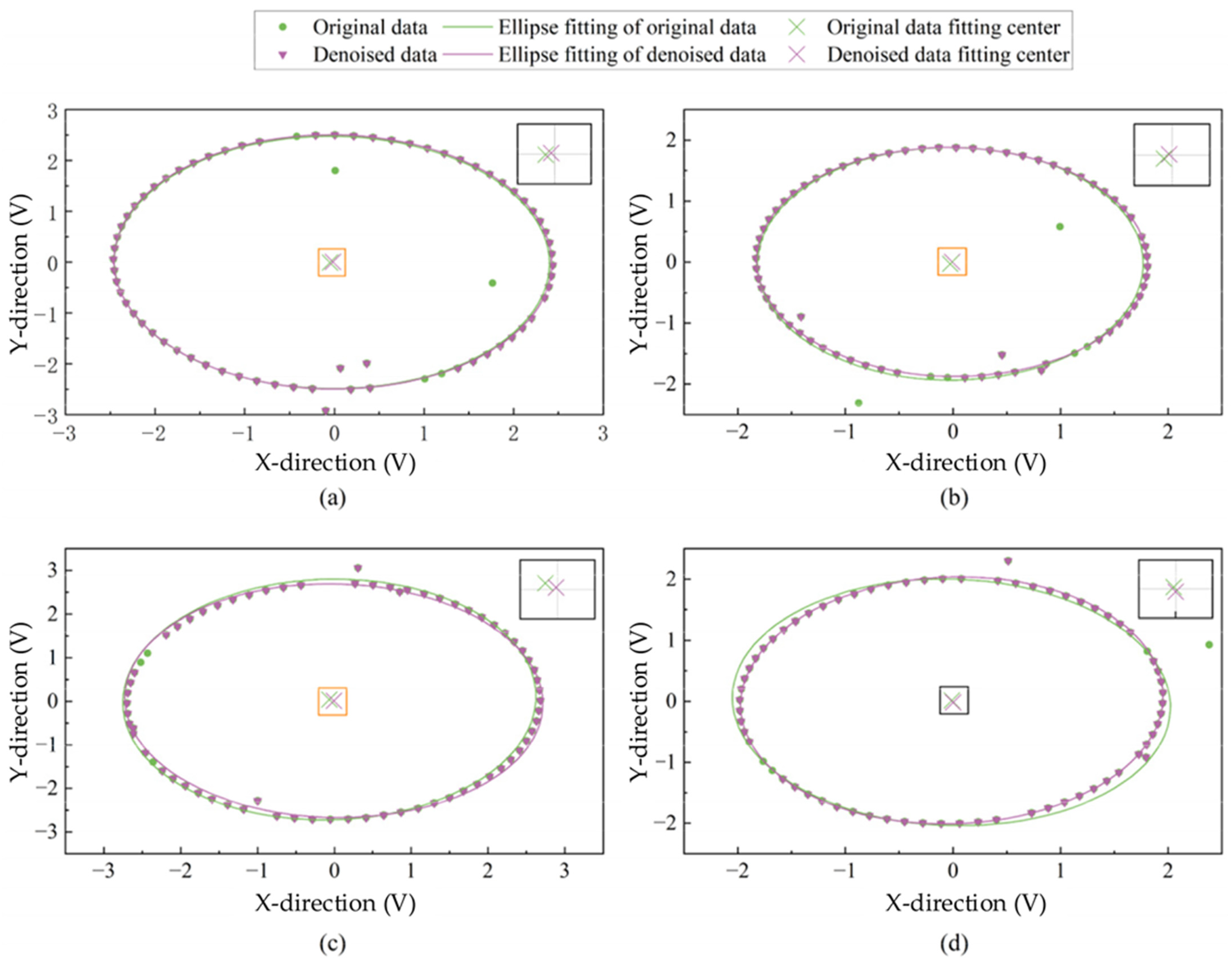
The azimuth angles of 60, 150, 240, and 330° are analyzed. OPTICS clustering is performed on the raw data of the X-axis and Y-axis of the magnetometer. The noise data in the raw data is deleted, and then the radial error is corrected using the least squares ellipse fitting. The results of the raw data fitting ellipse and the noise removal fitting ellipse are shown in Figure 6. As can be seen from Figure 6, OPTICS can effectively identify and eliminate singular values in the original data. After removing the noise, the fitted ellipse is more centralized (The enlarged image in the upper right corner is more intuitive), reducing the hard magnetic interference error.

Figure 6. OPTICS-based radial denoising and ellipse fitting results at different azimuth angles: (a) 60°, (b) 150°, (c) 240°, and (d) 330°.

The parameters of the fitted ellipse after noise removal are shown in Table 1. Parameters d and e determine the position of the ellipse center and characterize the presence of hard magnetic interference in the radial direction. Parameters a and c primarily control the length and ratio of the ellipse’s major axes, determining the ellipse’s shape. Parameter b reflects the ellipse’s tilt relative to the coordinate axis. Parameters a, b, and c together characterize the effect of soft magnetic interference on the magnetic field distribution. Parameter f controls the overall offset of the ellipse in the coordinate plane. Since the ellipse’s center deviates from the origin and its major axis direction and proportions vary, the elliptical parameters obtained after noise removal indicate significant magnetic interference in the radial direction of the magnetic field data. Using these elliptical parameters and Equation (16), radial correction can be applied to the original data.

Table 1. Ellipse fitting parameters.

Angle	a	b	c	d	e	f
60°	0.1625	0.0048	0.1554	0.0045	0.0017	0.9741
150°	0.2791	0.0076	0.2600	0.0061	0.0022	0.9244
240°	0.1290	0.0067	0.1360	0.0167	0.0109	0.9821
330°	0.2317	0.0174	0.2283	0.0069	0.0075	0.9454

3.2.2. Magnetic Interference Correction for the Single-Axis MSA Method

Since the single-axis MSA method is a one-dimensional optimization problem that only requires solving for the sensor error of the Z-axis, the Brent method is employed to address this problem. The optimization objective is to minimize the value of Equation (30), which represents the total variance of the vertical and horizontal magnetic field components. The Brent algorithm performs parabolic interpolation with a fallback to golden-section search, allowing efficient convergence without requiring gradient information. The search range for the optimization was set to [−5, 5], and the convergence tolerance was defined as 1 × 10⁻⁶ to ensure both stability and precision of the solution. The maximum number of iterations was set to 100 to guarantee sufficient convergence while maintaining computational efficiency.

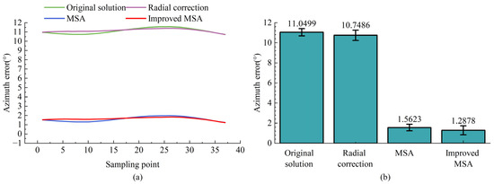
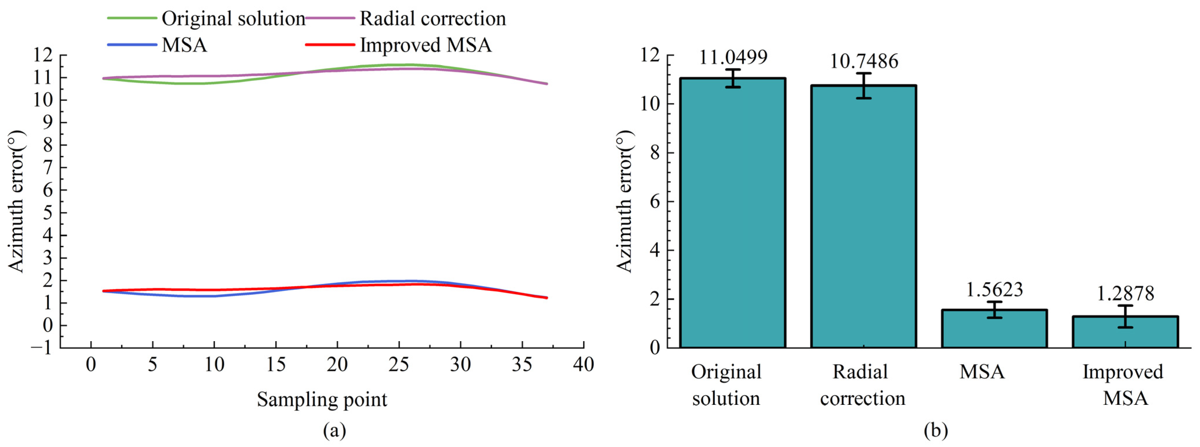
Taking the data at an azimuth angle of 60° as an example, the azimuth is calculated based on the raw data, the ellipse-fitted data, the MSA method, and the improved MSA method. The resulting azimuth polyline and error bar plots are shown in Figure 7.

Figure 7. Azimuth error analysis at 60°: (a) azimuth calculation error; (b) error metrics analysis.

Figure 7 presents the comparative results of azimuth error analysis at 60°. As shown in Figure 7a, both the raw solution and the radial correction exhibit large errors exceeding 10°, indicating that simple radial compensation cannot effectively suppress axial interference. By contrast, the MSA introduces a constrained optimization model that incorporates wellbore trajectory constraints to mitigate cross-coupling effects, reducing the azimuth error to approximately 1°. Building upon this, the improved MSA further enhances correction stability and accuracy through adaptive weighting of multi-station data, yielding more consistent error control. Figure 7b quantitatively compares the mean azimuth errors at 30°, showing that MSA and the improved MSA reduce the errors from 11.0499° and 10.7486° to 1.5623° and 1.2878°, respectively. These results demonstrate that introducing trajectory constraints and optimization in MSA significantly improves the robustness and applicability of azimuth correction.

3.2.3. MSA Method Integrated with GPR

The error data from the improved MSA method is used as the dataset, containing error data at 30, 60, 120, 150, 210, 240, and 300°, for a total of N = 582 data samples. The triaxial accelerometer and triaxial magnetometer data G_x, G_y, G_z, B_x, B_y and B_z measured by the inclinometer are selected as the input feature matrix X∈R^nx6. The measurement error A_error∈Rⁿ calculated by the corresponding improved MSA method is selected as the output target vector. The predicted error is then used to compensate for the azimuth. The dataset is split into training and test sets with a 7:3 ratio, and the input features and output targets are standardized. The ARD kernel function is used to automatically learn the importance of different input features, achieving feature screening and weighting.

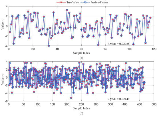
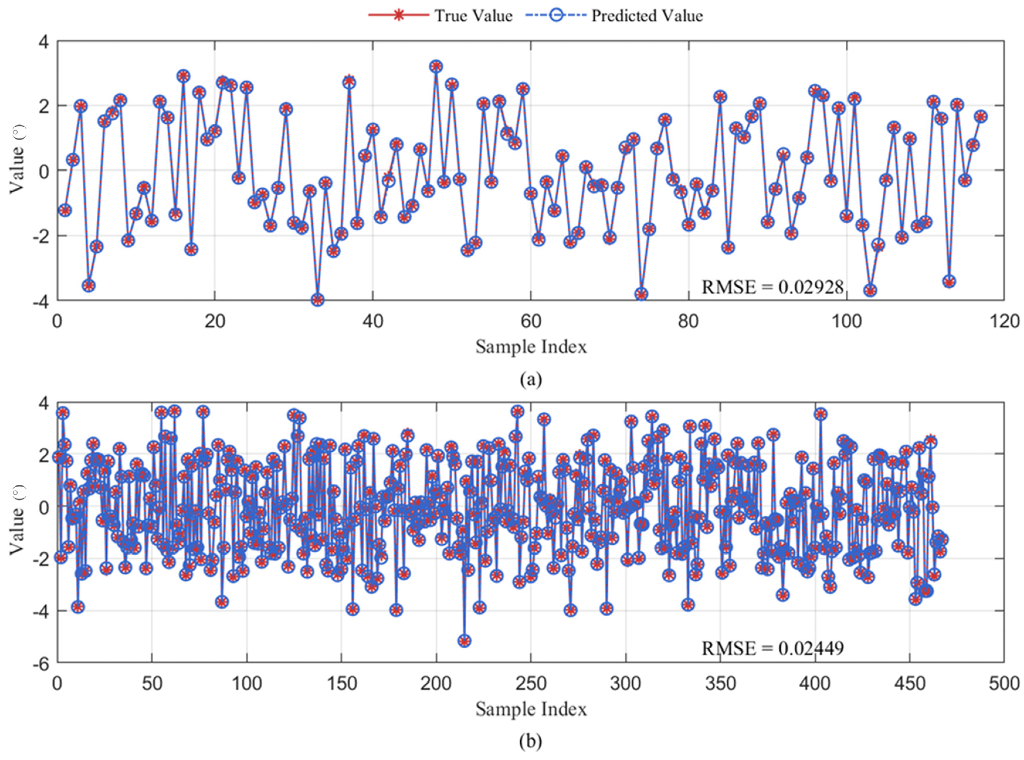
Specifically, after training the data using GPR, the prediction results for both the training and test sets are compared. As shown in Figure 8, the predicted values closely match the experimental values, indicating that the model accurately captures the error distribution patterns. As can be seen from Table 2, on the test set, the RMSE is only 0.02928, while the RMSE of the training set is 0.02449, both at very low levels. This demonstrates that the model not only fits the training data well but also exhibits excellent generalization performance on unseen data. Overall, the results confirm that the proposed method achieves high accuracy and robustness in the error compensation task.

Figure 8. Prediction results of the proposed model: (a) test set; (b) training set.

Table 2. Comparison of test set and training set indicators.

Dataset	R2	MAE
Test set	0.99972	0.02001
Train set	0.99991	0.01637

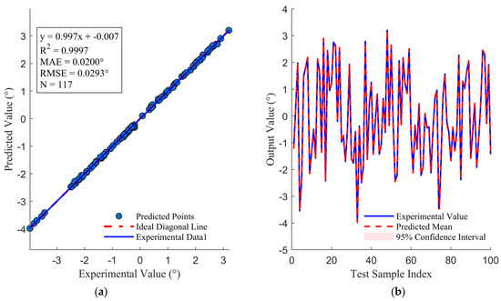
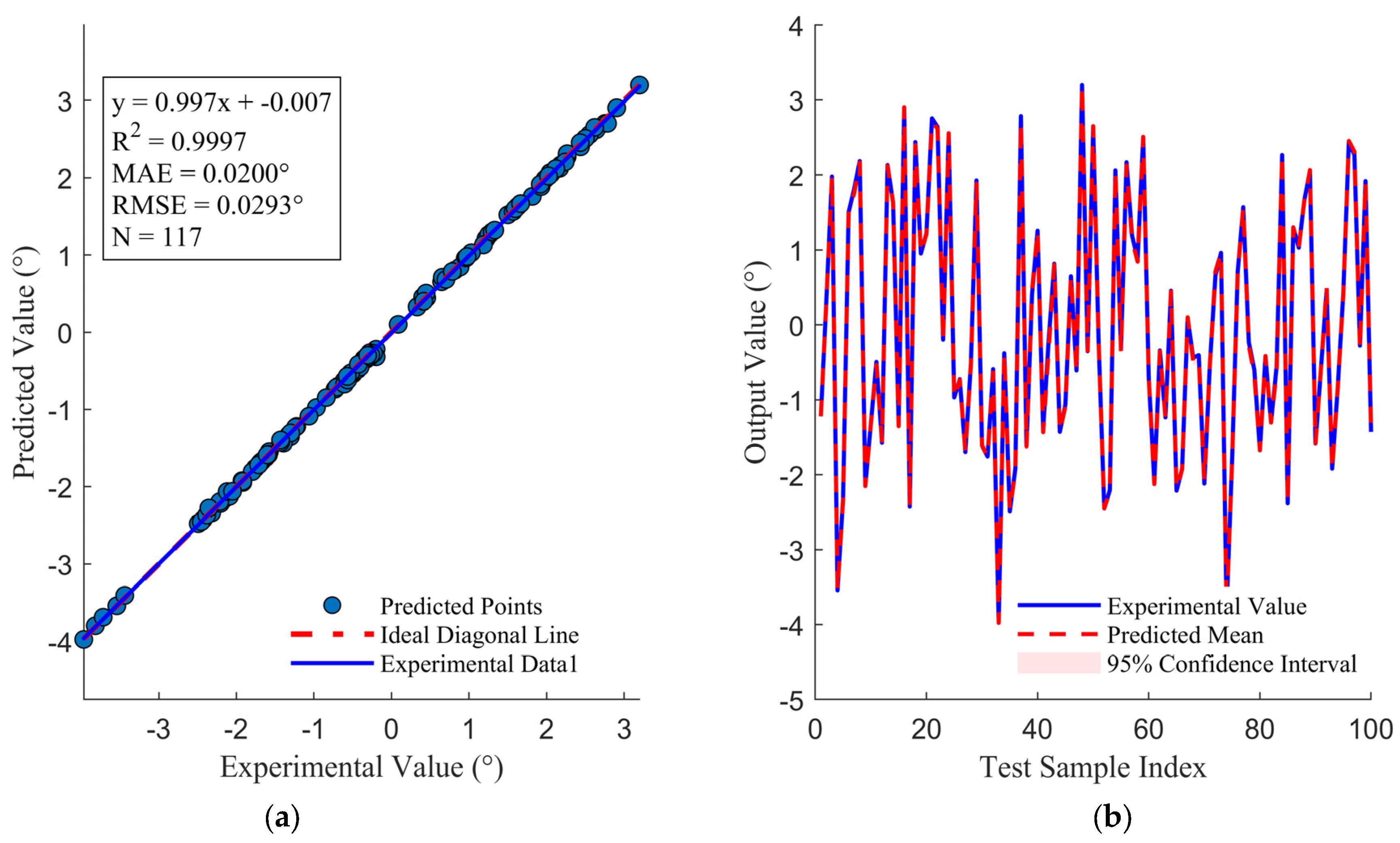
Moreover, to gain deeper insight into the prediction stability and uncertainty, the consistency between the predicted and experimental values is further analyzed. Figure 9a presents a scatter plot comparing the predicted and experimental values, where the data points lie almost entirely along the ideal diagonal, indicating that the model achieves very high overall fitting accuracy. Figure 9b shows a comparison of the first 100 test samples, demonstrating that the predicted curve nearly coincides with the experimental values curve and that the 95% confidence interval is extremely narrow. This indicates that the model can stably correct nonlinear errors and provides reliable uncertainty quantification for the predictions. These results further confirm the applicability and robustness of the proposed method under complex magnetic interference conditions.

Figure 9. Prediction performance and uncertainty analysis of the proposed model: (a) predicted vs. experimental values; (b) prediction results with 95% confidence interval (first 100 samples).

By extracting the weights of the ARD kernel, as shown in Table 3, it is observed that the weight of the B_z feature is significantly lower than those of the other five input features. This indicates that this feature plays a key role in the model and fully confirms that the magnetic interference from the magnetized casing mainly originates from the axial component.

Table 3. Length dimensions of different features.

Gx	Gy	Gz	Bx	By	Bz
7.93	6.52	13.38	7.88	10.23	0.068

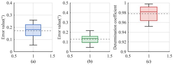
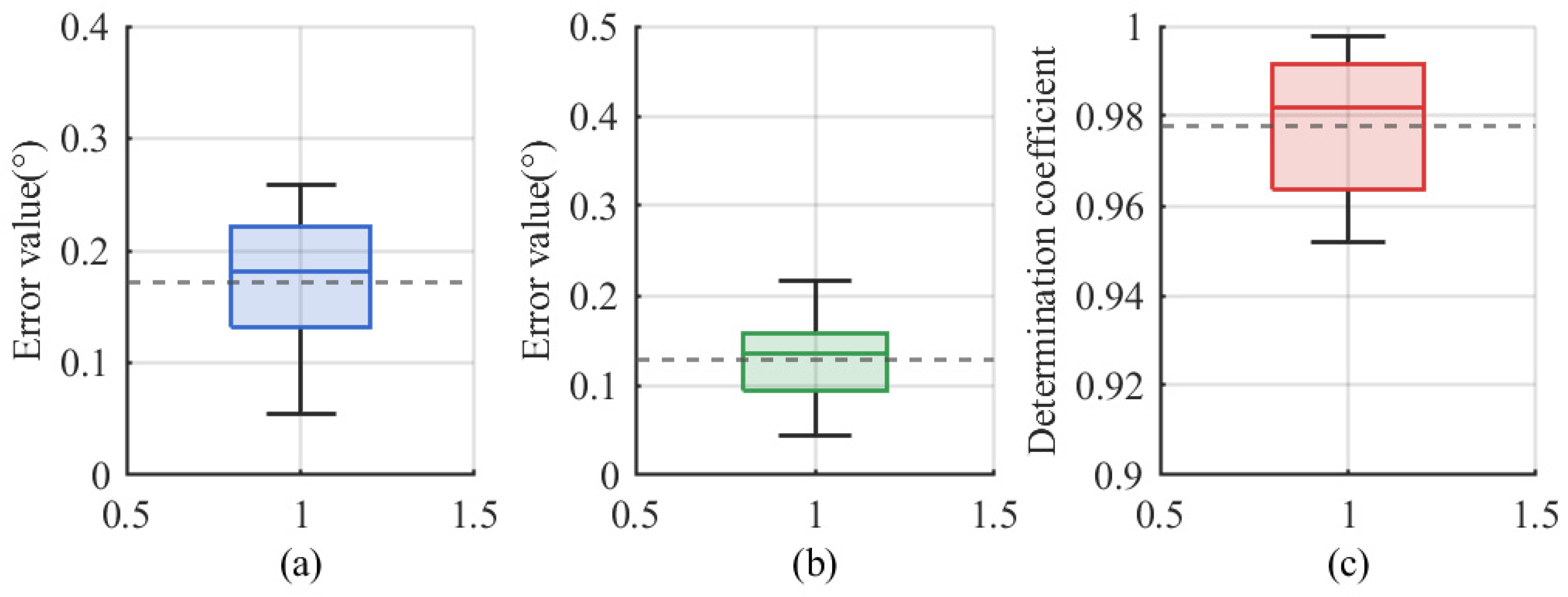
To further verify the generalization capability of the GPR model and rule out the possibility of overfitting, a five-fold group cross-validation was conducted using the complete dataset (N = 582). Each fold contained approximately 116 samples, with group partitioning performed according to the measurement azimuths to prevent data leakage between neighboring samples. The results of the five-fold cross-validation yielded an average RMSE = 0.17 ± 0.07°, MAE = 0.13 ± 0.06°, and R² = 0.98 ± 0.02. These results indicate that the GPR model maintains high accuracy and strong generalization capability without signs of overfitting.

The narrow interquartile ranges in the corresponding box-plot statistics, as shown in Figure 10, further confirm that the model effectively captures the nonlinear error distribution in complex magnetic environments. Meanwhile, the consistently low RMSE and MAE values demonstrate that the proposed GPR model achieves high prediction accuracy and strong generalization capability without any signs of overfitting.

Figure 10. Statistical evaluation of the GPR model performance based on 5-fold group cross-validation: (a) RMSE; (b) MAE; (c) R².

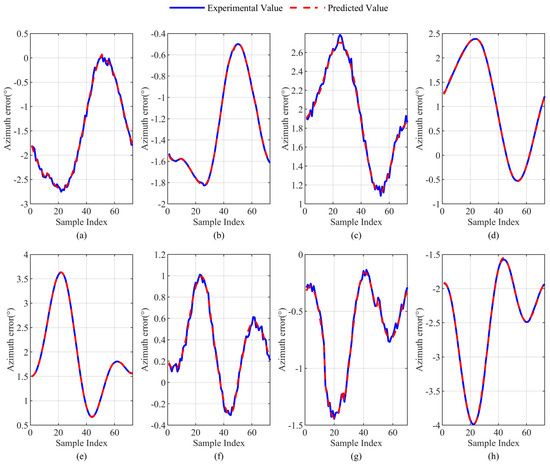
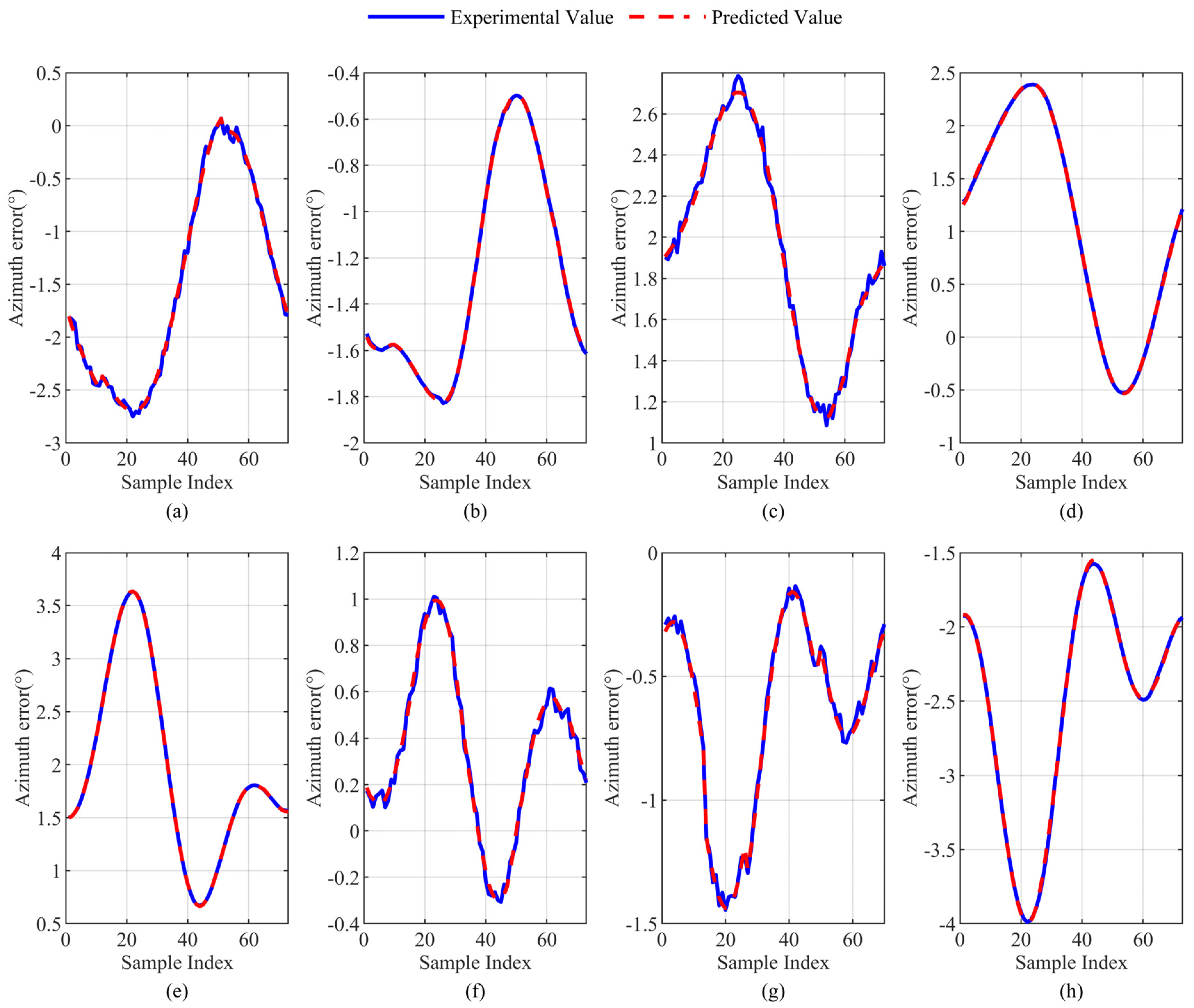
The trained GPR model is used to predict the original data, and the prediction results are denormalized. The resulting error value curve is shown in Figure 11. It can be clearly seen that the trained model can well predict the experimental value’s error value, and the curve fluctuation trends are basically consistent.

Figure 11. Comparison between predicted and experimental values at different azimuth angles: (a) 30°, (b) 60°, (c) 120°, (d) 150°, (e) 210°, (f) 240°, (g) 300°, and (h) 330°.

The specific error metrics are presented in Table 4 and Table 5. It can be observed that the GPR method achieves mean errors below 0.04° and standard deviations within 0.03° across all eight azimuth angles, significantly outperforming the other methods and demonstrating high accuracy and stability. In comparison, the improved MSA shows slight improvement over the original MSA at certain azimuths, but the mean errors remain between 0.4° and 2.5°, with noticeably larger standard deviations. The radial correction and raw calculation methods generally exhibit errors above 5° with considerable fluctuations. Overall, these results indicate that GPR possesses clear advantages in both accuracy and stability.”

Table 4. Comparison of eight azimuth error means.

Solution Method	30°	60°	120°	150°	210°	240°	300°	330°
GPR	0.0350°	0.0037°	0.00293°	0.0078°	0.0031°	0.0260°	0.0223°	0.0096°
Improved MSA	1.5157°	1.2878°	1.9505°	1.2257°	1.9586°	0.4194°	1.3017°	2.5343°
MSA	1.9215°	1.5623°	2.1958°	1.4746°	1.6175°	0.3548°	1.1524°	2.2698°
Radial correction	6.4126°	10.7486°	9.2150°	5.1922°	9.1233°	10.2753°	8.6803°	2.8303°
Original solution	6.7684°	11.0499°	9.5347°	5.7332°	9.2485°	11.2113°	8.8511°	3.0654°

Table 5. Comparison of eight azimuth error standard deviations.

Solution Method	30°	60°	120°	150°	210°	240°	300°	330°
GPR	0.0272°	0.0028°	0.0204°	0.0056°	0.0024°	0.0167°	0.0153°	0.0079°
Improved MSA	0.9443	0.4490	0.5118	0.8297	0.8759	0.2741	0.9364	0.7381
MSA	0.5695	0.3331	0.3659	0.5787	0.6401	0.2389	0.9580	0.5931
Radial correction	0.8328	0.5152	0.4107	1.1350	0.9596	0.2683	0.5867	0.6621
Original solution	0.4965	0.3639	0.3044	0.6627	0.7040	0.2530	0.5491	0.5313

4. Conclusions

During the Measurement-While-Drilling process in horizontal wells, the raw data often contain outliers and noise due to the complex downhole geomagnetic environment and the magnetization effects of the drilling tools. In this work, the Ordering Points to Identify the Clustering Structure clustering algorithm is combined with ellipse fitting to identify and remove outliers, effectively suppressing radial magnetic interference and enhancing azimuth stability under complex well conditions.

Building upon this, a constrained optimization model based on the improved Multi-Station Analysis method is proposed to mitigate axial interference by introducing wellbore trajectory constraints and reducing cross-coupling effects, thereby controlling the mean azimuth error within 2.5° and ensuring high stability and applicability.

Furthermore, Gaussian Process Regression is employed to model and compensate for residual nonlinear errors. By leveraging its advantages in nonlinear fitting and uncertainty quantification, the method accurately captures the error distribution and achieves robust compensation across various azimuths.

From an engineering perspective, the proposed three-stage correction framework comprising noise suppression, constrained optimization, and nonlinear compensation can be seamlessly integrated with existing Measurement-While-Drilling tools without additional hardware modification, enabling real-time azimuth correction and trajectory monitoring. By improving trajectory accuracy and reducing recalibration requirements, the method enhances operational efficiency and provides practical value for directional drilling applications in complex magnetic environments.

References

- Holditch, S.A. Unconventional Oil and Gas Resource Development—Let’s Do It Right. J. Unconv. Oil Gas Resour. 2013, 1–2, 2–8. [Google Scholar] [CrossRef] [Scilit]
- Zang, Y.; Wang, Q.; Wang, W.; Zhang, H.; Su, K.; Wang, H.; Li, M. Research on Drillability Prediction of Shale Horizontal Wells Based on Nonlinear Regression and Intelligent Optimization Algorithm. Processes 2025, 13, 3021. [Google Scholar] [CrossRef] [Scilit]
- Cheng, W.; Hu, S.; Zhang, M.; Song, H.; Zhang, G.; Chen, Y. Near-Vertical Attitude Determination Based on Balance Correction. IEEE Trans. Instrum. Meas. 2021, 70, 1–9. [Google Scholar] [CrossRef] [Scilit]
- Yang, C.; Zeng, Q.; Xiong, Z.; Yang, J. IMU/Magnetometer-Based Azimuth Estimation with Norm Constraint Filtering. Sensors 2024, 24, 2982. [Google Scholar] [CrossRef] [Scilit] [PubMed]
- Du, S.; Huang, C.; Ma, X.; Fan, H. A Review of Data-Driven Intelligent Monitoring for Geological Drilling Processes. Processes 2024, 12, 2478. [Google Scholar] [CrossRef] [Scilit]
- Wang, F.; Kobina, F. The Influence of Geological Factors and Transmission Fluids on the Exploitation of Reservoir Geothermal Resources: Factor Discussion and Mechanism Analysis. Reserv. Sci. 2025, 1, 3–18. [Google Scholar] [CrossRef] [Scilit]
- Wu, J.; Ansari, U. From CO2 Sequestration to Hydrogen Storage: Further Utilization of Depleted Gas Reservoirs. Reserv. Sci. 2025, 1, 19–35. [Google Scholar] [CrossRef] [Scilit]
- Li, Q. Reservoir Science: A Multi-Coupling Communication Platform to Promote Energy Transformation, Climate Change and Environmental Protection. Reserv. Sci. 2025, 1, 1–2. [Google Scholar] [CrossRef] [Scilit]
- Wu, P.; Wei, M. Magnetization Influence Analysis of the Casing and Drill Pipe in Shale Gas Dual Horizontal Well Rotating Magnet Ranging System Drilling Process. Energy Sci. Eng. 2020, 8, 3186–3199. [Google Scholar] [CrossRef] [Scilit]
- Li, H.; Cao, C. Magnetic Compass Calibration Based on Ellipse Fitting Algorithm Using DBSCAN. Electron. Meas. Technol. 2019, 42, 65–68. (In Chinese) [Google Scholar]
- Miu, L.; Wu, Z.; Zhou, Z.; Li, Z. Ellipse Fitting Error Compensation Method for Magnetic Compass Based on an Improved OPTICS Algorithm. J. Chin. Inert. Technol. 2022, 30, 174–180. (In Chinese) [Google Scholar]
- Bulychenkov, K. Improving Multistation Analysis of MWD Directional Magnetic Surveys. In Proceedings of the SPE Arctic and Extreme Environments Technical Conference and Exhibition, Moscow, Russia, 15–17 October 2013; SPE: Moscow, Russia, 2013. Paper SPE-166865-MS. [Google Scholar] [CrossRef] [Scilit]
- Gebre-Egziabher, D.; Hayward, R.C.; Powell, J.D. A Low-Cost GPS/Inertial Attitude Heading Reference System (AHRS) for General Aviation Applications. In Proceedings of the IEEE 1998 Position Location and Navigation Symposium, Palm Springs, CA, USA, 20–23 April 1996; pp. 518–525. [Google Scholar] [CrossRef] [Scilit]
- Kok, M.; Hol, J.D.; Schön, T.B. Using Inertial Sensors for Position and Orientation Estimation. arXiv 2017, arXiv:1704.06053. [Google Scholar] [CrossRef] [Scilit]
- Li, Y.; Yang, G. Error Compensation of Three-Axis Magnetometer Based on BP Neural Network. Measurement 2019, 134, 468–475. [Google Scholar]
- Sun, Z.; Zhao, J.; Shi, Z.; Yu, S. Soft Sensing of Magnetic Bearing System Based on Support Vector Regression and Extended Kalman Filter. Mechatronics 2014, 24, 186–197. [Google Scholar] [CrossRef] [Scilit]
- Solin, A.; Kok, M.; Wahlström, N.; Schön, T.B.; Särkkä, S. Modeling and Interpolation of the Ambient Magnetic Field by Gaussian Processes. IEEE Trans. Robot. 2018, 34, 1112–1127. [Google Scholar] [CrossRef] [Scilit]
- Viset, F.; Helmons, R.; Kok, M. An Extended Kalman Filter for Magnetic Field SLAM Using Gaussian Process Regression. Sensors 2022, 22, 2833. [Google Scholar] [CrossRef] [Scilit]
- Edridge, T.; Kok, M. Mapping the Magnetic Field Using a Magnetometer Array with Noisy Input Gaussian Process Regression. In Proceedings of the 2023 26th International Conference on Information Fusion (FUSION 2023), Charleston, SC, USA, 26–29 June 2023; IEEE: New York, NY, USA, 2023; pp. 1–7. [Google Scholar] [CrossRef] [Scilit]
- Liu, Z.; Lei, K.; Song, J.; Li, L.; Li, T. A Designed Calibration Approach for the Measurement-While-Drilling Instrument. Appl. Sci. 2023, 13, 61. [Google Scholar] [CrossRef] [Scilit]
- Yang, Y.; Li, F.; Gao, Y.; Mao, Y. Multi-Sensor Combined Measurement While Drilling Based on the Improved Adaptive Fading Square Root Unscented Kalman Filter. Sensors 2020, 20, 1897. [Google Scholar] [CrossRef] [Scilit]
- Song, H.; Huang, H.; Zhang, J.; Qu, D. A New Measurement-While-Drilling System Based on Inertial Technology. Adv. Mech. Eng. 2018, 10. [Google Scholar] [CrossRef] [Scilit]
- Guo, T.; Cheng, W.; Zhang, Y.; Chen, W.; Liu, X.; Chen, X. Azimuth Calibration Based on Equal Angle Balance Correction Algorithm for Measurement-While-Drilling System. Measurement 2024, 224, 113891. [Google Scholar] [CrossRef] [Scilit]
- Tra, V.; Kim, J.; Khan, S.A.; Kim, J.-M. Bearing Fault Diagnosis under Variable Speed Using Convolutional Neural Networks and the Stochastic Diagonal Levenberg-Marquardt Algorithm. Sensors 2017, 17, 2834. [Google Scholar] [CrossRef] [Scilit]
- Brooks, A.G.; Gurden, P.A.; Noy, K.A. Practical Application of a Multiple-Survey Magnetic Correction Algorithm. In Proceedings of the SPE Annual Technical Conference and Exhibition, New Orleans, LA, USA, 27–30 September 1998; SPE: Richardson, TX, USA, 1998. Paper SPE-49060. [Google Scholar] [CrossRef]
- Gebre-Egziabher, D.; Elkaim, G.H.; David Powell, J.; Parkinson, B.W. Calibration of Strapdown Magnetometers in Magnetic Field Domain. J. Aerosp. Eng. 2006, 19, 87–102. [Google Scholar] [CrossRef] [Scilit]
- Weston, J.; Ledroz, A. All-Attitude Gyrocompass Tool Offers Significant Enhancement in Survey Accuracy over the Highest Performance MWD Magnetic Systems. In Proceedings of the SPE/IADC Middle East Drilling Technology Conference and Exhibition, Abu Dhabi, United Arab Emirates, 26–28 January 2016; SPE: Richardson, TX, USA, 2016. Paper SPE-178254-MS. [Google Scholar] [CrossRef] [Scilit]
- Ren, X.; Liu, S. Calibration of MEMS Accelerometers and Magnetometers for Rotor UAV Attitude Estimation. In Proceedings of the International Conference on Chemical, Material and Food Engineering, Chongqing, China, 29–31 July 2015; Atlantis Press: Paris, France, 2015; pp. 742–745. [Google Scholar] [CrossRef] [Scilit]
- Fitzgibbon, A.; Pilu, M.; Fisher, R.B. Direct Least Square Fitting of Ellipses. IEEE Trans. Pattern Anal. Mach. Intell. 1999, 21, 476–480. [Google Scholar] [CrossRef] [Scilit]
- Ester, M.; Kriegel, H.-P.; Sander, J.; Xu, X. A Density-Based Algorithm for Discovering Clusters in Large Spatial Databases with Noise. In Proceedings of the Second International Conference on Knowledge Discovery and Data Mining (KDD’96), Portland, OR, USA, 2–4 August 1996; AAAI Press: Menlo Park, CA, USA, 1996; pp. 226–231. [Google Scholar]
- Subramani, K.; Velkov, A.; Ntoutsi, I.; Kroger, P.; Kriegel, H.-P. Density-Based Community Detection in Social Networks. In Proceedings of the 2011 IEEE 5th International Conference on Internet Multimedia Systems Architecture and Application (IMSAA), Bangalore, India, 12–13 December 2011; IEEE: New York, NY, USA, 2011; pp. 1–8. [Google Scholar] [CrossRef] [Scilit]
- Takebayashi, T.; Miyagusuku, R.; Ozaki, K. Development of Magnetic-Based Navigation by Constructing Maps Using Machine Learning for Autonomous Mobile Robots in Real Environments. Sensors 2021, 21, 3972. [Google Scholar] [CrossRef] [Scilit]
- Kirk, P.D.W.; Stumpf, M.P.H. Gaussian process regression bootstrapping: Exploring the effects of uncertainty in time course data. Bioinformatics 2009, 25, 1300–1306. [Google Scholar] [CrossRef] [Scilit]
- Girard, A.; Murray-Smith, R. Gaussian Processes: Prediction at a Noisy Input and Application to Iterative Multiple-Step Ahead Forecasting of Time-Series. In Switching and Learning in Feedback Systems; Lecture Notes in Computer, Science; Murray-Smith, R., Shorten, R., Eds.; Springer: Berlin/Heidelberg, Germany, 2005; Volume 3355, pp. 158–184. [Google Scholar]
- Ounpraseuth, S.T. Gaussian Processes in Machine Learning. J. Am. Stat. Assoc. 2008, 103, 429. [Google Scholar] [CrossRef] [Scilit]
- Williams, C.K.I.; Rasmussen, C.E. Gaussian Processes for Regression. In Proceedings of the 9th International Conference on Neural Information Processing Systems (NIPS’95), Denver, CO, USA, 4–8 December 1995; MIT Press: Cambridge, MA, USA, 1995; pp. 514–520. [Google Scholar]
- Ghoshal, S.; Roberts, S. Extracting Predictive Information from Heterogeneous Data Streams Using Gaussian Processes. Algorithmic Financ. 2016, 5, 21–30. [Google Scholar] [CrossRef] [Scilit]
- Seeger, M. Gaussian Processes for Machine Learning. Int. J. Neural Syst. 2004, 14, 69–106. [Google Scholar] [CrossRef] [Scilit]
Disclaimer/Publisher’s Note: The statements, opinions and data contained in all publications are solely those of the individual author(s) and contributor(s) and not of MDPI and/or the editor(s). MDPI and/or the editor(s) disclaim responsibility for any injury to people or property resulting from any ideas, methods, instructions or products referred to in the content. |
© 2025 by the authors. Licensee MDPI, Basel, Switzerland. This article is an open access article distributed under the terms and conditions of the Creative Commons Attribution (CC BY) license (https://creativecommons.org/licenses/by/4.0/).