Dynamic Response of Fracture Networks and the Evolution of Waterflood Fronts During Fracture-Flooding

Abstract

This study investigates the dynamic response of fracture networks and the evolution of waterflood fronts during fracture-flooding in low-permeability and tight reservoirs. By establishing a discrete fracture model that incorporates geomechanical heterogeneity and natural fractures, and utilizing the Barton-Bandis criterion to describe fracture stress-sensitive behavior, the fracture-flooding process was simulated and analyzed under two scenarios: considering versus ignoring the time-varying stress effect. The results demonstrate that when the time-varying stress effect is considered, fracture conductivity gradually recovers with increasing injection pressure, as the elevated fluid pressure within the fractures reduces the effective normal stress, promoting elastic dilation of the fracture aperture. This is evidenced by the average conductivity coefficient increasing from 0.4 (near-closure) to 0.99 (fully open) during the injection period. This recovery mechanism promotes a “wall-imbibition-dominated” flow pattern. In contrast, neglecting this effect leads to a “fracture-tip-breakthrough-dominated” mode, causing poor front uniformity. Quantitative analysis of the front morphology confirms this improvement: the perimeter-to-area ratio decreased from 2.507 to 1.647, and the coefficient of variation dropped from 0.490 to 0.324. This research provides an important theoretical basis for optimizing fracture-flooding operations and enhancing oil recovery.

1. Introduction

Currently, the focus of oil and gas resource development is gradually shifting towards unconventional reservoirs such as low-permeability, ultra-low-permeability, extra-low-permeability, tight, and shale formations [1,2,3]. For medium-to-high permeability (>10 mD) reservoirs [4] and low-permeability (1–10 mD) [5] reservoirs, conventional well pattern waterflooding can still meet development requirements. For reservoirs with extremely low permeability, such as tight reservoirs (0.001–0.1 mD) [6] and shale (<0.001 mD) [7], economic development to a certain extent can also be achieved by employing horizontal wells with volumetric fracturing to stimulate the reservoir [8]. However, for reservoirs with permeability ranging between that of low-permeability and tight reservoirs (0.1–1 mD), significant challenges arise. On one hand, conventional waterflooding development is problematic due to the low permeability, which makes water injection difficult. This hinders the effective propagation of displacement pressure, leading to poor replenishment of reservoir energy [9]. On the other hand, the injectivity of conventional waterflooding can be severely impaired over time by formation damage mechanisms, such as inorganic scaling induced by water incompatibility, which further reduces near-wellbore permeability and exacerbates injection challenges [10]. Furthermore, injected water tends to channel through high-permeability streaks, resulting in extensive ineffective circulation [11]. In contrast, the horizontal well volumetric fracturing technique can effectively stimulate the reservoir. However, its high investment cost leads to poor economic returns [12]. Additionally, its applicability is often limited in geologically complex conditions and smaller-scale reservoirs, making it difficult to deploy on a large scale.

Aiming at the shortcomings of existing development methods, fracture-flooding technology [13] is emerging as a promising alternative. This technique utilizes conventional waterflooding well patterns and employs high-pressure, high-volume injection combined with periodic shut-in periods. It not only creates a series of hydraulic fractures near the injection wellbore [14], effectively enhancing formation injectivity and helping to establish an effective displacement pressure system, but also improves oil mobilization from the matrix through high-pressure imbibition. An optimal fracture-flooding process aims to achieve uniform imbibition, where injected water primarily enters the matrix through the fracture walls, resulting in a more uniform, approximately circular waterflood front that maximizes sweep efficiency [15]. However, the effectiveness of the fracture-flooding process is highly dependent on the dynamic response characteristics of the natural fracture network. During the cyclic injection and production process, the fracture network undergoes significant changes in effective stress, leading to dynamic variations in its opening/closure state and conductivity [16]. This time-dependent stress process directly controls the dominant flow paths of the fracture-flooding fluid and the uniformity of the flood front advancement, consequently impacting the ultimate recovery efficiency [17].

Current research on fracture-flooding stimulation includes the following studies: Wang et al. [18,19] conducted full-cycle simulations of fracture propagation near the injection well, fluid seepage, and subsequent production during fracture-flooding using the Displacement Discontinuity Method (DDM) and the Embedded Discrete Fracture Model (EDFM). Their approach, which combines Bayesian algorithms with history matching optimization, can yield fracture-flooding parameters directly applicable in the field. However, a limitation is their assumption of homogeneous reservoir mechanical properties, failing to account for geomechanical heterogeneity in real reservoirs and the influence of natural fractures on fracture propagation. Furthermore, while considering dynamic fracture propagation, their model did not incorporate the dynamic changes in fracture properties during the fracture-flooding process. Xu et al. [20], using commercial numerical simulation software coupled with a dual-porosity/dual-permeability (DPDP) model, analyzed the impact of permeability distribution, permeability contrast, and injection volume on fracture-flooding performance. However, their study only considered areal heterogeneity and neglected vertical reservoir heterogeneity. Additionally, the use of the DPDP model led the authors to simplify the fracture network, preventing an effective representation of the dynamic propagation range of fractures and the time-dependent nature of fracture network properties. Zhao [21] utilized the tNavigator commercial numerical simulator with a dual-permeability model to compare different scenarios involving parameters such as injection volume, fracture parameters, and shut-in time. Nevertheless, this study also did not consider the influence of heterogeneity, particularly the distribution of natural fractures, on fracture network propagation. Wang et al. [22], employing a dual-permeability model, considered fracture stress-sensitivity and reservoir property anisotropy to conduct a comparative analysis between fracture-flooding and conventional waterflooding. However, the analysis primarily used conceptual models, and the applicability of their conclusions to real-world cases requires further verification. Su et al. [23] performed fluid-solid coupling simulations using ABAQUS 2022 to model fracture propagation during fracture-flooding, coupled with a dual-permeability model to establish a link between fracture geometry and flow parameters. But their work did not account for vertical reservoir heterogeneity or the influence of the natural fracture network system on the morphology of fracture-flooding-induced fractures. Cordero et al. [24] established a fracture classification standard, using the Discrete Fracture Model (DFM) for large-scale fractures and the Dual-Porosity/Dual-Permeability (DPDP) model for small-to-medium-scale fractures. They also incorporated the time-dependent nature of fracture properties by developing dynamic equations for fracture aperture and permeability. However, their methodology cannot model the dynamic fracture propagation process and fails to represent multiphase flow processes occurring in actual reservoirs.

Overall, existing numerical models predominantly rely on dual-porosity/dual-permeability (DPDP) models to characterize complex fracture systems. These methods involve significant simplifications of the fracture network structure, making it difficult to accurately represent the complex fracture morphology created during the fracture-flooding process and its time-dependent dynamic evolution. These limitations, namely the inability to accurately represent complex fracture morphology and its dynamic evolution, restrict the reliability of these models in predicting phenomena such as competitive propagation among multiple fractures and fluid exchange behavior [25,26,27]. Furthermore, most studies oversimplify the geomechanical characteristics of the reservoir, neglecting the controlling effect of reservoir heterogeneity—particularly the spatial variability of mechanical properties and the distribution of natural fracture systems—on the propagation paths of hydraulic fractures and the resulting fracture network morphology. Existing models often assume a homogeneous reservoir or only consider areal heterogeneity, overlooking the interaction between vertical heterogeneity and the natural fracture network. This leads to deviations in predicting the dynamic fracture propagation behavior during fracture-flooding [28,29]. Consequently, for fracture-flooding optimization research to be more aligned with con conditions, it is crucial to place greater emphasis on the spatial heterogeneity of reservoir mechanical parameters, including vertical layering characteristics and the distribution of natural fractures. This should be combined with embedding more realistic discrete fracture networks using the Discrete Fracture Model (DFM) and coupling it with an Unconventional Fracture Model (UFM) [30,31], which is based on the extended Finite Element Method (XFEM) principle, to more accurately simulate the dynamic propagation of fracture-flooding-induced fractures and their interaction with the natural fracture system. Simultaneously, unstructured grids offer a significantly superior capability for characterizing the geometry of complex fracture networks compared to traditional DPDP models, thus presenting a distinct advantage in fracture-flooding simulations [32,33].

Based on a systematic analysis of existing research achievements and shortcomings, this paper focuses on an in-depth investigation of the dynamic response behavior of natural fracture networks and the formation mechanisms of dominant flow channels during the fracture-flooding process, which is accompanied by time-dependent stress effects. Firstly, a heterogeneous geomechanical model integrating multiple geological factors—such as natural fracture distribution, in situ stress field, reservoir pressure, and permeability field—is constructed based on the Discrete Fracture Model (DFM). Subsequently, by incorporating the Unconventional Fracture Model (UFM), the propagation geometry and spatial distribution of the fracture network induced by fracture-flooding under multi-factor heterogeneous geological conditions are simulated. Furthermore, by introducing the Barton-Bandis criterion [34], a dynamic coupling model for pore pressure, in situ stress, and fracture properties is established to characterize the spatiotemporal evolution of fracture aperture and permeability during the fracture-flooding process. Finally, based on the structural parameters of an actual well group, parameterized scenarios are analyzed to examine the distribution patterns of fracture-flooding injection water, comparing cases that consider versus neglect the time-dependent stress effects on fracture properties.

2. Geomechanics-Flow Coupling Theoretical Model

2.1. Description of the Geological Model

The reservoir block exhibits a high degree of natural fracture development (Figure 1). The distribution of these natural fractures follows a pattern of higher density in the central area and lower density on the two flanks. The properties of the natural fracture network are presented in Table 1. The model grid dimensions are 222 cells in the I-direction, 179 cells in the J-direction, and 20 cells in the K-direction, resulting in a total of 794,760 grid cells. With an average grid width of 10 m and an average grid thickness of 1 m, the model achieves a balance between seismic resolution and computational efficiency. The model has an average thickness of 20.2 m and an average permeability of 1.01 mD, which places its characteristics between those of an ultra-low permeability reservoir and a tight oil reservoir. The reservoir property ranges are presented in Table 2.

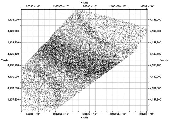
Figure 1. Conceptual model of natural fracture distribution in the reservoir: This model is based on the typical characteristics of an ultra-low permeability sandstone reservoir in the B435 Block (anonymized designation) of the Shengli Oilfield.

Table 1. Range of values for natural fracture properties.

Natural Fracture Properties	Value
Length range	2–25 m
Average length	12.36 m
Orientation range	15°–105°
Average Orientation	62.5° (northeast)
Average spacing	8.35 m

Table 2. Range of values for basic reservoir physical properties.

Reservoir Physical Properties	Value
Range of porosity	0.087–0.219
Average porosity	0.155
Range of permeability	0.544–1.472 mD
Average permeability	1.01 mD
Range of water saturation	0.267–0.598
Average water saturation	0.411
Pressure	29.36 MPa
Average maximum horizontal stress	45 MPa
Average minimum horizontal stress	42 MPa
Average overburden stress	65 MPa

2.2. Simulation of Fracture Network Propagation from a Fracture-Flooding Well

Based on the field geological model, a simulation of fracture network propagation was conducted for the well group containing the X25 well. Figure 2 illustrates the distribution of natural fracture density along the direction of the maximum horizontal stress near the X25 well. The X25 well is situated between two zones of high natural fracture density. Consequently, natural fractures exert a significant influence on the morphology of the fracture-flooding-induced fracture network from the X25 well.

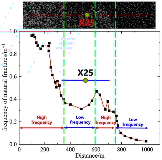
Figure 2. The spatial distribution of natural fracture density along the direction of the maximum horizontal principal stress near Well X25 (The red line marks the maximum principal stress direction; The green line shows the alignment between the upper fracture map and the lower density curve).

Specifically, within the high-density zone on the left, the natural fractures have an average angle of 27.39° and a median angle of 23.96° relative to the direction of the maximum horizontal stress. In the central low-density zone, the average angle is 25.78° with a median of 21.98°. For the high-density zone on the right, the average angle is 31.39° and the median is 29.74°. The orientation of natural fractures in the central area is closer to the direction of the maximum horizontal stress. Furthermore, the fracture density in the central area is lower than that on the left and right sides (Central: 0.314, Left: 0.561, Right: 0.470). This lower density implies a reduced probability of the propagating fracture-flooding fractures encountering natural fractures when extending through the central zone. Therefore, the natural fractures in the central area have a lesser impact on altering the propagation direction of the fracture-flooding fractures compared to the influence exerted by the natural fractures on either side. Figure 3 illustrates the distribution of angles between the orientations of natural fractures and the direction of the maximum principal stress at different locations near Well X25.

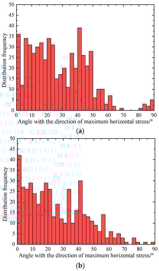
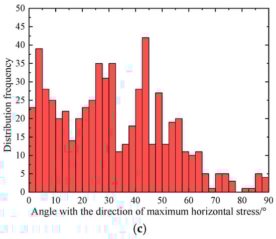
Figure 3. Distribution of the angle between natural fracture orientation and maximum principal stress direction at different locations: (a) left side; (b) center; (c) right side.

Figure 4 displays the specific morphology of the fracture-flooding network. Driven by the orientation of the maximum horizontal stress, the overall azimuth of the fracture-flooding network is 60° northeast. Due to the heterogeneity in natural fracture distribution, the fracture network exhibits a pattern of numerous branch fractures on the two flanks and fewer branches in the central section. The average angle between the fracture network and the direction of the maximum horizontal stress is 19.99°. The minimum angles are primarily associated with the main fractures in the central area, ranging from 0° to 0.05°. In contrast, the maximum angles are predominantly found within the complex fracture networks on the flanks, with the largest angle reaching 89.95°. The propagation length of the fracture-flooding network is 307.89 m along the direction of the maximum horizontal stress and 110.07 m along the direction of the minimum horizontal stress. Table 3 lists the average height, width, and total surface area of the fracture-flooding network.

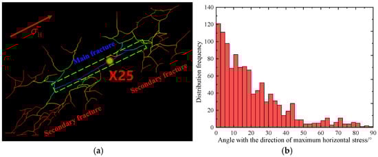
Figure 4. Modeling result: Geometry of the fracture-flooding network simulated by the Unconventional Fracture Model (UFM), showing (a) the morphology and (b) the angle distribution relative to the maximum horizontal stress. (a) Fracture network morphology diagram of fracture-flooding fractures. (b) Distribution of the angle between the fracture network and the maximum horizontal stress direction.

Table 3. Other parameters of the fracture-flooding fracture network.

Other Parameters of the Fracture-Flooding Fracture Network	Value
Average fracture height	9.90 m
Average fracture width	3.52 mm
Total fracture surface area	20,914.56 m2

2.3. A Coupled Model of Fracture Nonlinear Deformation and Seepage Based on the Barton-Bandis Criterion

During fracture-flooding injection, the rapid injection of a large volume of water in a short period creates a series of hydraulic fractures near the wellbore. However, fracture-flooding differs from conventional fracturing as proppant is typically not added during the operation. Consequently, after the fractures are activated by the injected water, they often lack effective proppant support. As the pressure within the fractures declines, the fractures gradually close, leading to a reduction in their permeability. However, this permeability reduction process is reversible. When water is injected again during a subsequent fracture-flooding cycle, the pressure inside the fractures increases, causing the fracture aperture to widen and permeability to be restored. Figure 5 illustrates this process of dynamic change in fracture conductivity.

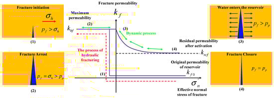
Figure 5. Schematic diagram of fracture nonlinear deformation according to the Barton-Bandis criterion.

To accurately characterize this critical physical process, this study introduces the empirical constitutive model developed by Barton and Bandis. Established based on extensive experimental data on rock fractures, this model effectively describes the nonlinear deformation behavior of fractures (primarily elastic opening) under normal stress. In terms of its physical mechanism, it more accurately reflects the true mechanical response of subsurface fractures compared to simplified models such as the linear spring model or the assumption of constant conductivity.

The core of the Barton-Bandis model lies in its definition of an empirical relationship among fracture normal stiffness $k_n$, normal stress ${\sigma }_n$ acting on the fracture, and fracture aperture (Equation (1)). The normal stiffness represents the fracture’s ability to resist deformation under normal stress (the stress acting perpendicular to the fracture plane) when no external force is applied (i.e., at zero stress state). It is quantitatively defined as the change in fracture aperture per unit change in normal stress.

$$k_n={\displaystyle \frac{d{\sigma }_n}{de}}$$

(1)

In the equation,

$k_n$: Fracture normal stiffness, MPa/m.

${\sigma }_n$: Fracture normal stress, MPa.

$e$: The change in aperture per unit change in normal stress, m.

The initial normal stiffness of a fracture can be calculated using an empirical Equation (2):

$$k_{n\mathrm{i}}=0.02\cdot {\displaystyle \frac{\mathrm{JCS}}{1\mathrm{MPa}}}+1.75\cdot \mathrm{JRC}\text{-}10$$

(2)

In the equation,

$k_{n\mathrm{i}}$: Initial normal stiffness, MPa/mm.

$\mathrm{JCS}$: Joint Compressive Strength, MPa.

$\mathrm{JRC}$: Joint Roughness Coefficient, dimensionless

10: A dimensionless fitting coefficient, dimensionless

Under normal stress, the closure behavior of a fracture exhibits a nonlinear hyperbolic characteristic. Therefore, based on the Barton-Bandis model, a relationship between normal stiffness and effective normal stress can be derived (Equation (3)) [35].

$$k_n=k_{n\mathrm{i}}{[1-{\displaystyle \frac{{\sigma }_n^{\prime }}{V_m{k}_{n\mathrm{i}}+{\sigma }_n^{\prime }}}]}^{-2}$$

(3)

In the equation,

${\sigma }_n^{\prime }$: Effective Normal Stress on the Fracture, MPa.

$V_m$: Maximum Closure: The mechanical behavior when the fracture aperture decreases to its limiting state (i.e., the fracture is nearly fully closed), m.

The effective normal stress on the fracture (Figure 6) can be calculated using Equations (4) and (5).

$${\sigma }_n^{\prime }={\sigma }_n-\alpha p_f$$

(4)

$${\sigma }_n={\displaystyle \frac{({\sigma }_H+{\sigma }_h)}{2}}+{\displaystyle \frac{({\sigma }_H-{\sigma }_h)}{2}}\cos (2\theta )$$

(5)

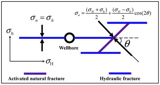
Figure 6. Schematic diagram of normal stress on fracture surface.

In the equation,

$p_f$: Intra-Fracture Fluid Pressure, MPa.

$\alpha$: Biot coefficient, dimensionless.

${\sigma }_H$: Maximum horizontal stress, MPa.

${\sigma }_h$: Minimum horizontal stress, MPa.

$\theta$: Angle between the fracture normal and the maximum horizontal stress orientation, °.

Based on the cubic law, a relationship between the hydraulic aperture and the conductivity (or flow capacity) of a fracture can be established (Equation (6)) [36].

$$e={(12k)}^{0.5}$$

(6)

Assuming the fracture permeability is $k_{hf}$ when the fracture reaches its maximum aperture $e_0$, the following Equation (7) holds true when the aperture changes to a specific value $e$:

$${\displaystyle \frac{e}{e_0}}={({\displaystyle \frac{12k_f}{12k_{hf}}})}^{0.5}$$

(7)

Based on the previous Equation (7), it can be further rearranged to obtain (Equation (8)):

$$k_f=k_{hf}{({\displaystyle \frac{e}{e_0}})}^2$$

(8)

When the fracture reaches its minimum aperture $e_m$ (fully closed), its conductivity $k_{rcf}$ can be calculated using the following Equation (9).

$$k_{rcf}=k_{hf}{({\displaystyle \frac{e_m}{e_0}})}^2$$

(9)

The minimum aperture of a fracture can be calculated based on the Barton-Bandis model (Equation (10)). A fracture with high wall roughness can still maintain a relatively high residual aperture even after it is fully closed. Figure 7 displays the residual aperture of fractures under different roughness conditions after complete closure.

$$e_m={\displaystyle \frac{e_0\cdot \mathrm{JRC}}{M+N\cdot \mathrm{JRC}}}$$

(10)

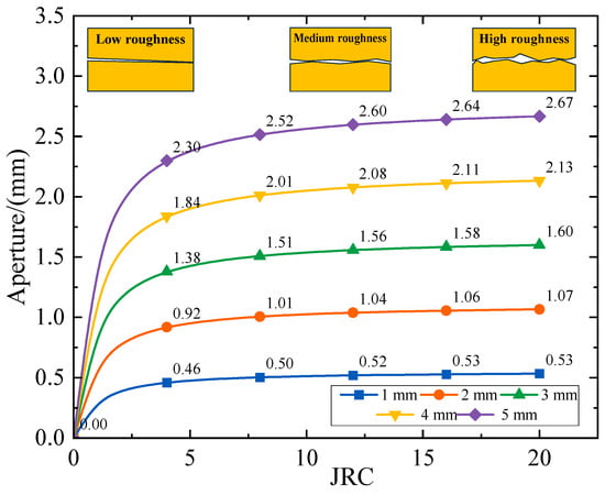
Figure 7. Aperture after complete closure under different roughness levels (Low roughness: JRC 0–4; Medium roughness: JRC 5–9; High roughness: JRC 10–14).

In the equation,

$M,N$: Empirical coefficient, $M=1.5$, $N=1.8$.

The hydraulic aperture of a fracture under varying stress conditions can be calculated by the following Equations (11)–(13).

$$e=e_0-V_j$$

(11)

$$V_j={\displaystyle \frac{{\sigma }_n^{\prime }}{k_n+\raisebox{1ex}{${\sigma }_n^{\prime }$}\!\left/ \!\raisebox{-1ex}{$V_m$}\right.}}$$

(12)

$$V_m=e_0-e_m$$

(13)

In the equation,

$V_j$: Closure Amount, m.

Therefore, the following condition must be added as a constraint to Equation (14):

$$k_f=k_{hf}{({\displaystyle \frac{e}{e_0}})}^2\ge k_{rcf}$$

(14)

Therefore, the variation in fracture conductivity with increasing normal stress under different intersection angles $\theta$ can be obtained, as shown in Figure 8.

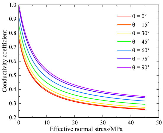
Figure 8. Variation in conductivity with effective normal stress under different angles.

The fracture aperture can be equivalently represented by the porosity of the fracture grid. Since there is no proppant filling inside the fracture-flooding-induced fractures, their absolute porosity can be considered as 1. Therefore, the fracture volume can be calculated using the following Equation (15).

$$V_f=e\cdot L\cdot H\cdot {\varphi }_f$$

(15)

In the equation,

$V_f$: Volume of the fracture, m³.

$L$: Length of the fracture, m.

$H$: Height of the fracture, m.

${\varphi }_f$: The porosity of the fracture is assumed to be equal to 1 in this context.

The volume of the unstructured grid used to represent the fracture (Equation (16)).

$$V_t=W\cdot L\cdot H$$

(16)

In the equation,

$W$: The width of the unstructured grid cell used to represent the fracture, m.

Based on Equation (17), the equivalent porosity of the fracture at different apertures can be calculated. Therefore, the variation in effective fracture porosity with increasing normal stress under different intersection angles $\theta$ can be obtained, as shown in Figure 9.

$${\varphi }_e={\displaystyle \frac{V_f}{V_t}}={\displaystyle \frac{e}{W}}$$

(17)

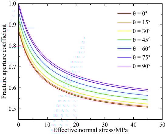
Figure 9. Variation in fracture aperture with effective normal stress under different angles.

3. Analysis of Dynamic Responses of Fracture Networks and Evolution Patterns of Waterflood Fronts at the Field Scale

3.1. Model Overview Introduction

To validate the effectiveness of the nonlinear deformation-flow coupling model for fracture-flooding fractures constructed in the previous section, this section conducts a case study utilizing actual well group production data. A comprehensive performance evaluation of the model is performed by comparing the simulation results with field-observed data. Figure 10 illustrates the sector model of the field fracture-flooding well group. The sector model contains 8 vertical wells, including one water injection well, X25 (the fracture-flooding well), and seven production wells.

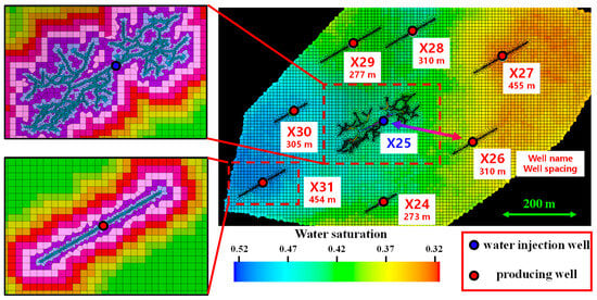
Figure 10. Coupled fracture network field block unstructured grid model (water saturation).

Based on the field production schedule, first, the seven production wells undergo depletion production for 6 months; subsequently, the seven production wells are shut in, and the fracture-flooding well begins fracture-flooding injection for energy replenishment over 6 months; finally, the fracture-flooding well is shut in, and the seven production wells are reopened for production for another 6 months.

The key parameters used in this numerical simulation (summarized in Table 4) are primarily based on actual field operations and fracture-flooding practices from the target reservoir block. For instance, the minimum bottom-hole pressure (MBHP) constraint for production wells, the water injection rate of 0.6 m³/min during the fracture-flooding period, and the cumulative injection volume of 40,000 m³ are all derived from optimized protocols validated through field practice in this block. The selection of these parameters aims to align the simulation conditions as closely as possible with real-world scenarios, thereby ensuring the reliability and practical relevance of the simulation results.

Table 4. Summary of key parameter values in numerical simulation.

Parameter	Value	Well Name	Hydraulic Fracture Length
Minimum Bottom Hole Pressure (MBHP)	15 MPa	X24	116.69 m
Duration of the First Depletion Production	180 days	X26	167.49 m
Fracture-flooding Duration	180 days	X27	207.22 m
Duration of the Second Depletion Production	180 days	X28	186.88 m
Water Injection Rate During Fracturing Period	0.6 m3/min	X29	227.55 m
Water Injection Rate During Conventional Waterflooding	300 m3/d	X30	121.73 m
Water Injection Volume	40,000 m3/d (Fracture-flooding) 20,000 m3/d (Water flooding)	X31	173.31 m

To address the differences in oil-water flow mechanisms within different regions of the reservoir, this paper establishes a relative permeability curve zoning model based on grid-type mapping. This model assigns distinct relative permeability curves according to the medium type represented by each grid cell: for grids characterizing fractures, the classic straight-line intersecting relative permeability curves are applied; for grids representing matrix rock blocks, the relative permeability relationships determined from onsite core flooding experiments are utilized. This approach effectively captures the flow heterogeneity inherent in the fracture-matrix dual-porosity system (Figure 11).

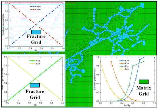
Figure 11. Relative permeability curves for different fracture grids in the model.

In terms of handling stress-sensitive characteristics, the model also adopts a differentiated approach based on the differences in medium types: for fracture grids, the previously derived nonlinear deformation governing equations for fractures are employed to dynamically describe their stress-sensitive behavior; for matrix grids, the elastic compression effect of rock pores is primarily considered, and corresponding stress-sensitive curves are constructed by incorporating the rock compressibility coefficient. This coupled treatment method significantly enhances the model’s accuracy in characterizing the stress-sensitive behavior of geological bodies and their physical rationality (Figure 12).

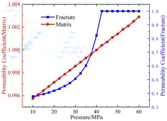
Figure 12. Stress sensitivity curves for fractures and matrix.

3.2. Spatiotemporal Evolution of Fracture Networks and Waterflood Fronts with Production Responses

A comparative analysis was conducted between two scenarios: one considering the stress sensitivity of the fracture network and the other neglecting it. The results indicate that after introducing the stress sensitivity effect, the aperture of the fracture network during the initial fracture-flooding stage is lower, leading to a significant reduction in flow conductivity. Under these conditions, the short-term high-intensity injection (864 m³/d) caused a rapid pressure buildup at the bottomhole of well X25. In contrast, when the time-varying stress effect is disregarded, the fracture network maintains a higher aperture without significant pressure accumulation.

During the fracture-flooding operation, an effective fracture network must be created around the wellbore. This requires the bottomhole pressure to consistently exceed the minimum horizontal principal stress (42 MPa) to ensure fracture initiation and propagation. Figure 13 shows the bottomhole pressure curves of the fracture-flooding well under the two scenarios. The simulation results demonstrate that in the model incorporating the time-varying stress effect, the bottomhole pressure remains above this threshold throughout the entire fracture-flooding process, satisfying the mechanical conditions for fracture formation. Conversely, in the model that ignores stress sensitivity, the bottomhole pressure never reaches the critical value required for fracture initiation.

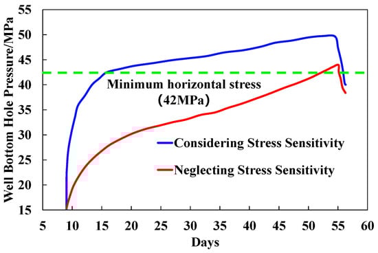
Figure 13. Bottom hole pressure curves under different stress sensitivity conditions.

The simulation results considering the time-varying stress effect show a higher degree of consistency with field observations, demonstrating that this model can more accurately reflect the dynamic evolution of the fracture network and the pressure response behavior during the fracture-flooding process.

When the time-varying stress effects of the fracture-flooding fracture network are considered, the fractures exhibit a small initial aperture and consequently low flow conductivity under the action of in situ horizontal stresses. As a result, during the initial stage of fracture-flooding, injected water struggles to propagate rapidly through the fracture network. The flow conductivity of the fractures demonstrates a trend of gradual improvement, propagating from the wellbore outwards towards the periphery during the fracture-flooding process. Simulation results indicate that as the fracture-flooding operation progresses from day 0 to day 30, the average flow conductivity coefficient of the fracture network increases continuously, rising from an initial value of 0.4 (near-closure state) to 0.67. By day 30, the entire fracture-flooding network has developed substantial overall flow capacity, enabling the injected water to effectively and rapidly propagate through the fracture grids, leading to a swift increase in the average pressure within the fracture network. Correspondingly, during the period from day 30 to day 45, the growth rate of the average flow conductivity coefficient accelerates significantly, ultimately recovering to 0.99 by the end of the fracture-flooding phase, indicating that the fracture network is nearly fully open (Figure 14).

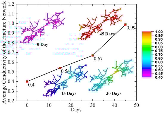
Figure 14. Average fracture network conductivity at different times during fracture-flooding.

When the time-varying stress effects of the fracture-flooding network are considered, the fractures exhibit a small initial aperture and consequently low flow conductivity under the action of in situ stresses. Simulation results indicate that as the fracture-flooding operation progresses, the average conductivity of the fracture network demonstrates a distinct two-stage recovery characteristic (Figure 14).

Initial Slow Recovery Stage (e.g., Injection Start-Day 30): During this stage, the average conductivity coefficient increased gradually from an initial value of 0.4 (near-closure state) to 0.67 by day 30. The underlying mechanism is that the initial injection pressure is primarily utilized to overcome the in situ stress and elevate the fluid pressure within the fractures, thereby reducing the effective normal stress that compacts them. The recovery of fracture aperture and conductivity is relatively slow during this pressure-building phase.

Subsequent Accelerated Recovery Stage (e.g., Day 30-Injection End): Once the internal fracture pressure accumulated to a critical level (around day 30), the growth rate of the conductivity coefficient accelerated markedly, rising rapidly from 0.67 at day 30 to 0.99 (nearly fully open) by the end of the injection period. This indicates significant elastic dilation of the fracture network under high internal pressure, whereby substantial overall flow capacity is established, enabling the effective and rapid propagation of injected water.

This dynamic recovery process of conductivity is directly coupled with and corroborates the downhole pressure response shown in Figure 13, where the bottomhole flowing pressure continuously rises and eventually exceeds the fracture propagation threshold. It clearly reveals the core physical mechanism of the fracture-flooding process: “pressure increase; reduction in effective stress; fracture dilation; recovery of conductivity”.

Under conditions where the time-varying stress effects of the fracture network are neglected, the conductivity of the fracture-flooding network remains high. Injected water advances rapidly along the fractures. Due to the low flow resistance in the main body of the fractures, the flow direction is primarily along the fracture length, with minimal leak-off through the fracture walls. When the injected water reaches the fracture tip, where propagation terminates, flow is obstructed, causing a significant volume of water to enter the reservoir matrix concentrated at the tip.

Conversely, when the time-varying stress effect is considered, the fracture-flooding fractures exhibit low initial conductivity. The injected water cannot be transported rapidly along the fracture length and instead accumulates within the fractures near the wellbore, causing pressure buildup. As the pressure inside the fractures gradually increases, the fracture aperture and conductivity increase, promoting forward flow along the fracture. Simultaneously, the elevated internal pressure also enhances the leak-off rate of the injected water through the fracture walls into the adjacent matrix.

Therefore, neglecting stress time-dependency results in the injected water primarily entering the matrix from the fracture tip during the fracture-flooding process. This can easily lead to uneven sweep efficiency, forming a waterflood front that advances outward starting from the fracture tip, making it difficult to achieve a more uniform sweep pattern. In contrast, when the time-varying stress effect is considered, the injected water primarily enters the matrix through the fracture walls. This is more conducive to displacing the remaining oil within the matrix blocks partitioned by the fracture network, leading to improved sweep efficiency.

Figure 15 illustrates the distribution patterns of water saturation during the fracture-flooding process under the two scenarios. In the initial stage (0–7 days), as injected water begins to enter the fractures, it primarily migrates along the fracture network in both cases, with only a small amount entering the matrix. When the time-varying stress effect is neglected, the propagation distance of the injected water within the fractures is longer (Figure 15d, 256 m), significantly greater than that observed in the scenario considering time-varying stress (Figure 15a, 160 m). During the mid-term stage (7–15 days), the influence of stress time-dependency on the sweep efficiency is not pronounced. This is because the injected water has not yet established significant connectivity with the production wells, avoiding large-scale water channeling or ineffective cycling. Furthermore, since the total injected water volume is identical in both scenarios, the swept area shows no substantial difference (Figure 16). Simulation results indicate that the effective sweep efficiency of the injected water throughout the entire fracture-flooding process is 0.246 and 0.237, respectively (the well group’s controlled area is 323,256.8 m²).

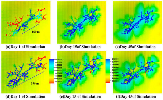
Figure 15. Waterfront positions at different times under two conditions ((a–c): considering stress time-dependency of fractures; (d–f): without considering stress time-dependency of fractures).

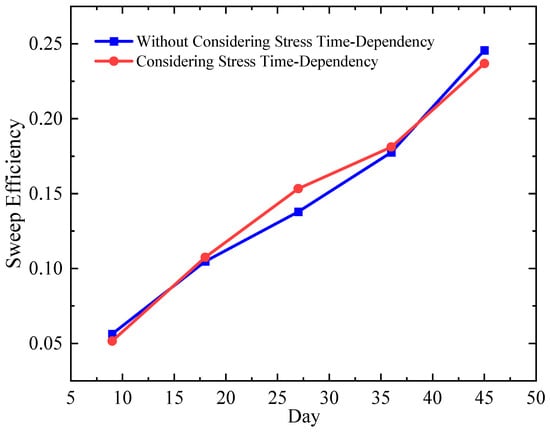
Figure 16. Water flooding sweep efficiency at different times under two conditions.

In the context of developing remaining oil via waterflooding in reservoirs, the uniformity of the waterflood front advancement significantly influences the ultimate recovery efficiency. A more uniform waterflood front implies that all points on the front are approximately equidistant from the injection well, representing equal propagation distances for the displacing water and indicating the absence of rapid water breakthrough along any specific direction. Consequently, an ideal waterflood front should exhibit a shape characteristic that approximates a circle as closely as possible (Figure 17). Based on this principle, the waterflood fronts under the two scenarios are analyzed. The first metric is the Perimeter-to-Area ratio (PA ratio) of the waterflood front. A more uniform advance, resulting in a shape closer to a circle, will yield a PA ratio closer to 1 (Equation (18)).

$$\mathrm{PA}ratio={\displaystyle \frac{P}{2\sqrt{\pi \cdot A}}}$$

(18)

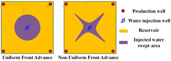
Figure 17. Schematic diagram of water flooding front uniformity.

In the equation,

$P$: Perimeter of the waterflood front, m.

$A$: Enclosed area of the waterflood front, m².

The second metric is the uniformity of the advancement velocity. If the waterflood front advances uniformly, the distances from various points on the front to the injection well should be similar. Therefore, this study calculates the distance from each point on the front to the well location using the Euclidean distance method. Subsequently, the mean and standard deviation of the sample dataset are computed. Finally, the coefficient of variation (CV) of the dataset is determined. The coefficient of variation eliminates the influence of the absolute numerical values and units of measurement, enabling a direct and fair comparison of the dispersion degree across different datasets (Equations (19)–(22)).

$$d_i=\sqrt{{(x_i-x_w)}^2+{(y_i-y_w)}^2}$$

(19)

$$\mu ={\displaystyle \frac{{\displaystyle \sum _{i=1}^N{d}_i}}{N}}$$

(20)

$$\sigma =\sqrt{{\displaystyle \frac{1}{N}}{\displaystyle \sum _{i=1}^N{(d_i-\mu )}^2}}$$

(21)

$$CV={\displaystyle \frac{\sigma }{\mu }}$$

(22)

In the equation,

$(x_i,y_i)$: The coordinate values of the i-th point on the waterflood front, m.

$(x_w,y_w)$: The Coordinate Values of the Injection Well, m.

$\mu$: The mean distance of all points to the injection well, m.

$\sigma$: The standard deviation of the sample dataset.

$CV$: The coefficient of variation (CV) of the sample dataset.

Figure 18 presents the calculation results for the two different scenarios. The results demonstrate that when the time-varying stress characteristics of fracture properties are considered, the uniformity of the waterflood front advancement is significantly improved. The perimeter-to-area ratio decreases from 2.507 to 1.647, and the coefficient of variation in the waterflood front is reduced from 0.490 to 0.324.

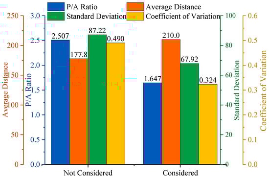
Figure 18. Computed values under two conditions.

The primary reason for this phenomenon is that when the time-varying stress effect on fracture properties is neglected, the injected water tends to preferentially enter the porous matrix from the fracture tips. This leads to a significantly greater advancement distance of the waterflood front at the fracture tips compared to the distance advanced from the fracture walls (Figure 19b), resulting in an irregular front morphology. In contrast, when the time-varying stress effect is incorporated, the injected water no longer enters the matrix solely from the fracture tips but enters simultaneously from multiple locations, including both the fracture walls and the tips (Figure 19a). Consequently, the advancement uniformity of the waterflood front is significantly superior to the former case, leading to a more ideal sweep efficiency.

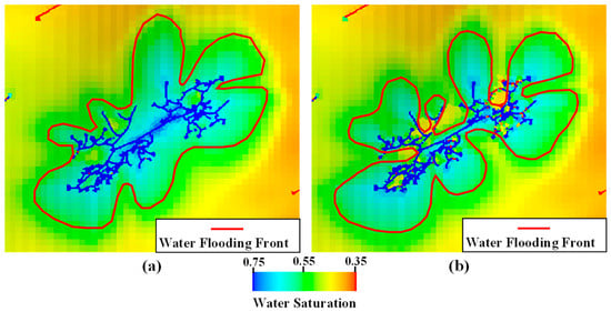
Figure 19. Water flooding front morphology under two conditions ((a): Considering Stress Time-Dependency; (b): Without Considering Stress Time-Dependency).

4. Conclusions

This study systematically investigated the dynamic response of fracture networks and the evolution patterns of waterflood fronts during fracture-flooding under time-varying stress effects. This was achieved by constructing a discrete fracture network model that incorporates geomechanical heterogeneity and natural fracture distribution, coupled with the Barton-Bandis criterion to describe nonlinear fracture deformation behavior. Through validation against actual well group production data and comparative scenario analysis, the following main conclusions are drawn:

The time-varying stress effect is a key mechanism controlling the dynamic evolution of conductivity in fracture-flooding networks. When this effect is considered, fractures are in a near-closed state under initial in situ stress, resulting in low initial conductivity (average conductivity coefficient of 0.4). As high-pressure injection proceeds, the pressure within the fractures gradually increases, leading to a reduction in the effective normal stress (as defined in Equations (4) and (5)). This stress reduction, governed by the nonlinear deformation relationship of the Barton-Bandis criterion (Equations (1)–(3) and (11)–(13)), dynamically recovers the fracture aperture and, consequently, the conductivity via the cubic law (Equation (6)). This process enables the bottomhole flowing pressure to effectively exceed the formation’s minimum horizontal principal stress (42 MPa), satisfying the mechanical conditions for fracture creation—a fundamental field observation that models neglecting this effect fail to replicate.

The spatiotemporal dynamic evolution of fracture conductivity directly determines the advancement mode and sweep uniformity of the waterflood front. The “wall-imbibition-dominated” mode, facilitated by the time-varying stress effect, results in a more uniform, approximately circular waterflood front. Conversely, neglecting the time-varying stress effect leads to a “fracture-tip-breakthrough-dominated” mode, producing a highly irregular front morphology prone to ineffective water cycling.

Quantitative evaluation demonstrates that considering the time-varying stress effect significantly improves the waterflood sweep efficiency. The incorporation of fracture stress sensitivity substantially enhances front uniformity, with the Perimeter-to-Area ratio improving from 2.507 to 1.647 and the Coefficient of Variation decreasing from 0.490 to 0.324. These metrics confirm a front shape closer to the ideal circle, effectively mitigating the adverse effects of preferential flow paths.

In summary, the time-varying stress effect on fracture properties and its coupling with reservoir geological heterogeneity must be fully considered in the numerical simulation and optimization of fracture-flooding processes. The coupled model and methodology established in this study can more accurately reveal the dynamic mechanisms of fracture-flooding, providing a scientific basis for decision-making in the efficient development of low-permeability and tight reservoirs.

References

- Hui, G.; Ren, Y.; Bi, J.; Wang, M.; Liu, C. Artificial intelligence applications and challenges in oil and gas exploration and development. Adv. Geo-Energy Res. 2025, 17, 179–183. [Google Scholar] [CrossRef]
- Zhang, Y.; Ji, Y.; Qi, M.; Dong, L.; Zhang, S.; Li, Y. Integrated detection of micro-pore structures and macro-mechanical responses for hydrate-bearing sediments. Adv. Geo-Energy Res. 2025, 17, 184–195. [Google Scholar] [CrossRef]
- Wei, Z.; Sheng, M.; Li, J.; Zhang, B.; Wang, B.; Li, G. Pressure diagnostics in hydraulic fracturing for unconventional completion optimization. Adv. Geo-Energy Res. 2025, 17, 196–211. [Google Scholar] [CrossRef]
- Emami-Meybodi, H.; Ma, M.; Zhang, F.; Rui, Z.; Rezaeyan, A.; Ghanizadeh, A.; Hamdi, H.; Clarkson, C.R. Cyclic gas injection in low-permeability oil reservoirs: Progress in modeling and experiments. SPE J. 2024, 29, 6217–6250. [Google Scholar] [CrossRef]
- Xiliang, L.; Hao, C.; Yang, L.; Yangwen, Z.; Haiying, L.; Qingmin, Z.; Xianmin, Z.; Hongbo, Z. Oil production characteristics and CO2 storage mechanisms of CO2 flooding in ultra-low permeability sandstone oil reservoirs. Pet. Explor. Dev. 2025, 52, 196–207. [Google Scholar] [CrossRef]
- Li, L.; Liu, Y.; Su, Y.; Niu, H.; Hou, Z.; Hao, Y. Integrated study on CO2 enhanced oil recovery and geological storage in tight oil reservoirs. Geoenergy Sci. Eng. 2024, 241, 213143. [Google Scholar] [CrossRef]
- Feng, Q.; Xu, S.; Xing, X.; Zhang, W.; Wang, S. Advances and challenges in shale oil development: A critical review. Adv. Geo-Energy Res. 2020, 4, 406–418. [Google Scholar] [CrossRef]
- Wei, B.; Qiao, R.; Hou, J.; Wu, Z.; Sun, J.; Zhang, Y.; Qiang, X.; Zhao, E. Multiphase production prediction of volume fracturing horizontal wells in tight oil reservoir during cyclic water injection. Phys. Fluids 2025, 37, 013304. [Google Scholar] [CrossRef]
- Chuan, C.; Huai, L.; Zhong, W. Analysis of pressures in water injection wells considering fracture influence induced by pressure-drive water injection. Pet. Reserv. Eval. Dev. 2023, 13, 686–694. [Google Scholar] [CrossRef]
- Khormali, A.; Ahmadi, S.; Aleksandrov, A.N. Analysis of reservoir rock permeability changes due to solid precipitation during waterflooding using artificial neural network. J. Pet. Explor. Prod. Technol. 2025, 15, 17. [Google Scholar] [CrossRef]
- Wei, Z.; Su, Y.; Yong, W.; Liu, B.; Zhang, J.; Zhou, W.; Liu, Y. A Novel Quantitative Water Channeling Identification Method of Offshore Oil Reservoirs. Processes 2024, 12, 2363. [Google Scholar] [CrossRef]
- Du, D.; Liu, P.; Ren, L.; Li, Y.; Tang, Y.; Hao, F. A Volume Fracturing Percolation Model for Tight Reservoir Vertical Wells. Processes 2023, 11, 2575. [Google Scholar] [CrossRef]
- Zhao, M.; Guo, X.; Wu, Y.; Dai, C.; Gao, M.; Yan, R.; Cheng, Y.; Li, Y.; Song, X.; Wang, X. Development, performance evaluation and enhanced oil recovery regulations of a zwitterionic viscoelastic surfactant fracturing-flooding system. Colloids Surf. A Physicochem. Eng. Asp. 2021, 630, 127568. [Google Scholar] [CrossRef]
- Cao, H.; Zhang, G.; Li, S.; Zhou, D.; Yu, C.; Sun, Q. Fracturing initiation and breakdown pressures in fracturing-flooding sandstone reservoirs. Rock Mech. Rock Eng. 2024, 1–18. [Google Scholar] [CrossRef]
- Moorman, E.D.; Xue, J.; Ibrahim, I.; Okeke, N.; Trabelsi, R.; Trabelsi, H.; Boukadi, F. Optimizing Intermittent Water Injection Cycles to Mitigate Asphaltene Formation: A Reservoir Simulation Approach. Processes 2025, 13, 2143. [Google Scholar] [CrossRef]
- Zhang, Q.; Wang, W.-D.; Su, Y.-L.; Chen, W.; Lei, Z.-D.; Li, L.; Hao, Y.-M. A semi-analytical model for coupled flow in stress-sensitive multi-scale shale reservoirs with fractal characteristics. Pet. Sci. 2024, 21, 327–342. [Google Scholar] [CrossRef]
- Zhang, J.; Standifird, W.; Roegiers, J.-C.; Zhang, Y. Stress-dependent fluid flow and permeability in fractured media: From lab experiments to engineering applications. Rock Mech. Rock Eng. 2007, 40, 3–21. [Google Scholar] [CrossRef]
- Wang, J.; Cui, C.; Wu, Z.; Qian, Y.; He, J. Optimization of Well Response Times in Fracturing-Flooding Using a Coupled Fluid-Solid Model for Heterogeneous Reservoirs. Geoenergy Sci. Eng. 2025, 254, 214022. [Google Scholar] [CrossRef]
- Cui, C.; Wang, J.; Qian, Y.; Li, J.; Lu, S. Fracturing–flooding for low-permeability oil reservoirs: A coupled model integrating DDM and black-oil model. Rock Mech. Rock Eng. 2025, 58, 4069–4089. [Google Scholar] [CrossRef]
- Xu, H.; Niu, B.; Huang, L.; Zhang, L.; Hao, Y.; Yue, Z. Study on the Influence Mechanisms of Reservoir Heterogeneity on Flow Capacity During Fracturing Flooding Development. Energies 2025, 18, 3279. [Google Scholar] [CrossRef]
- Zhao, Z.; Jiang, S.; Lei, T.; Wang, J.; Zhang, Y. Optimization of key parameters of fracturing flooding development in offshore reservoirs with low permeability based on numerical modeling approach. J. Mar. Sci. Eng. 2025, 13, 282. [Google Scholar] [CrossRef]
- Wang, X.; Yu, W.; Xie, Y.; He, Y.; Xu, H.; Chu, X.; Li, C. Numerical simulation of the dynamic behavior of low permeability reservoirs under fracturing-flooding based on a dual-porous and dual-permeable media model. Energies 2024, 17, 6203. [Google Scholar] [CrossRef]
- Su, Y.; Jia, M.; Yao, Y.; Tong, G.; Xian, Y.; Wang, W. Investigation of fully coupled fracture propagation and oil–water two-phase flow mechanisms in fracturing flooding. Phys. Fluids 2025, 37, 056611. [Google Scholar] [CrossRef]
- Cordero, J.A.R.; Sanchez, E.C.M.; Roehl, D. Integrated discrete fracture and dual porosity-dual permeability models for fluid flow in deformable fractured media. J. Pet. Sci. Eng. 2019, 175, 644–653. [Google Scholar] [CrossRef]
- Rueda, J.; Mejia, C.; Noreña, N.; Roehl, D. A three-dimensional enhanced dual-porosity and dual-permeability approach for hydromechanical modeling of naturally fractured rocks. Int. J. Numer. Methods Eng. 2021, 122, 1663–1686. [Google Scholar] [CrossRef]
- Nie, R.-S.; Meng, Y.-F.; Jia, Y.-L.; Zhang, F.-X.; Yang, X.-T.; Niu, X.-N. Dual porosity and dual permeability modeling of horizontal well in naturally fractured reservoir. Transp. Porous Media 2012, 92, 213–235. [Google Scholar] [CrossRef]
- Yang, S.; Lei, Y.; Chen, D.; Gao, L.; Wang, M.; Zheng, Q. Permeability model of coalbed methane reservoir with heterogeneous rough dual-porosity medium considering multiple gas flow mechanisms. Powder Technol. 2025, 464, 121174. [Google Scholar] [CrossRef]
- Xiong, D.; He, J. Evaluation of a complex fracture network in deep coalbed methane reservoir considering natural fracture tensile and shear failure. Phys. Fluids 2025, 37, 036601. [Google Scholar] [CrossRef]
- Li, N.; Zhu, S.; Li, Y.; Zhao, J.; Long, B.; Chen, F.; Wang, E.; Feng, W.; Hu, Y.; Wang, S. Fracturing-flooding technology for low permeability reservoirs: A review. Petroleum 2024, 10, 202–215. [Google Scholar] [CrossRef]
- Weng, M.-C.; Peng, C.-H.; Le, H.-K.; Shiu, W.-J.; Fang, C.-H. Discrete element analysis of hydraulic stimulation in a slate geothermal reservoir using the ubiquitous foliation model. Geomech. Geophys. Geo-Energy Geo-Resour. 2024, 10, 37. [Google Scholar] [CrossRef]
- Lavoine, E.; Davy, P.; Darcel, C.; Munier, R. A discrete fracture network model with stress-driven nucleation: Impact on clustering, connectivity, and topology. Front. Phys. 2020, 8, 9. [Google Scholar] [CrossRef]
- Bahrainian, S.S.; Daneh Dezfuli, A.; Noghrehabadi, A. Unstructured grid generation in porous domains for flow simulations with discrete-fracture network model. Transp. Porous Media 2015, 109, 693–709. [Google Scholar] [CrossRef]
- Mehrdoost, Z. Multiscale finite volume method with adaptive unstructured grids for flow simulation in heterogeneous fractured porous media. Eng. Comput. 2022, 38, 4961–4977. [Google Scholar] [CrossRef]
- Li, X.; Zhu, B.; Xiao, W. A modified Barton-Bandis normal closure model for infilled rock joint. Environ. Earth Sci. 2025, 84, 403. [Google Scholar] [CrossRef]
- Bandis, S.; Lumsden, A.; Barton, N. Fundamentals of rock joint deformation. Int. J. Rock Mech. Min. Sci. Geomech. Abstr. 1983, 20, 249–268. [Google Scholar] [CrossRef]
- Barton, N.; Bandis, S.; Bakhtar, K. Strength, deformation and conductivity coupling of rock joints. Int. J. Rock Mech. Min. Sci. Geomech. Abstr. 1985, 22, 121–140. [Google Scholar] [CrossRef]
Disclaimer/Publisher’s Note: The statements, opinions and data contained in all publications are solely those of the individual author(s) and contributor(s) and not of MDPI and/or the editor(s). MDPI and/or the editor(s) disclaim responsibility for any injury to people or property resulting from any ideas, methods, instructions or products referred to in the content. |
© 2025 by the authors. Licensee MDPI, Basel, Switzerland. This article is an open access article distributed under the terms and conditions of the Creative Commons Attribution (CC BY) license (https://creativecommons.org/licenses/by/4.0/).