Integrated Hybrid Modelling and Surrogate Model-Based Operation Optimization of Fluid Catalytic Cracking Process

Abstract

Fluid Catalytic Cracking (FCC) is one of the most important conversion processes in oil refineries, widely used to convert high-boiling, high-molecular-weight hydrocarbon components from crude oil into more valuable products like gasoline and diesel. Advanced simulation and optimization technologies are critical for improving the operational efficiency and economic performance of the FCC process. First-principles-based simulators rely on parameter estimation and are computationally intensive, making them unsuitable for online optimization. In recent years, with the development of deep learning, data-driven models have made significant progress in FCC modeling. However, due to their black-box nature and difficulty with extrapolation, they are rarely used for optimization. To bridge this gap, we propose an integrated framework that combines hybrid modeling and surrogate model-based optimization. This approach combines plant and simulation data to train a multi-task learning prediction model, which then serves as a surrogate for operational optimization. Validated on a large-scale FCC unit in southern China, the model predicts product yields with an error margin of under 4.84% for all products. Following optimization, yields of LNG, gasoline, and diesel rose by an average of 0.10 wt%, 1.58 wt%, and 1.05 wt%, respectively, resulting in a 3.67% increase in product revenues. This highlights the substantial potential of this framework for industrial applications.

1. Introduction

Fluid Catalytic Cracking (FCC) is one of the key processes in the refining industry, transforming heavy fractions of crude oil into lighter and more valuable products such as gasoline and diesel [1]. During this high-temperature process, catalysts break down long-chain hydrocarbons into shorter ones [2]. FCC enhances fuel yields for refineries, playing an essential role in fulfilling the market demand for light hydrocarbon fuels [3]. In the petrochemical industry, the efficiency of the FCC process and the quality of its products directly impact the economic benefits and market competitiveness of refining enterprises [4]. Due to the complex and variable composition of crude oil and constantly changing demands for various products, precise simulation and optimization of the FCC process are extremely important [5].

In the era of smart manufacturing, advanced modeling and optimization are essential for the FCC process [6]. Process modeling helps engineers understand complex chemical reactions and fluid dynamics [7], which is significant for implementing process improvements, enhancing product quality, conserving energy and raw materials, and reducing operational costs [8]. Moreover, optimizing the FCC process ensures the production of products that better meet fluctuating market demands and operate in a more environmentally friendly manner [9], thus bringing significant economic and social benefits [10].

Classic methods for modeling the FCC process include rigorous mechanistic models founded on first principles. A major group of models are lumped kinetics models, which simplify complex reaction networks by grouping similar chemical species into “lumps” or pseudo-components [11]. The earliest model is a 3-lump model proposed by Weekman et al. [12,13] to predict the feedstock conversion rate and gasoline yield. Later, Arbel et al. reported a 10-lump model that allows feed and catalyst characterization based on laboratory experiments [14]. More recently, Ebrahimi et al. constructed a 9-lump model containing 18 kinetic parameters and 2 parameters for the catalyst de-activation for the vacuum gas oil (VGO) catalytic cracking process [15]. Another group of models is molecular kinetic models. Yang et al. presented a structure-oriented lumping (SOL) combined with the Monte Carlo (MC) method to simulate the secondary reaction process of FCC [16].

Kinetic parameters are crucial for the prediction accuracy of such models. Therefore, lots of researchers have explored parameter estimation methods for constructing mechanistic models. For example, John et al. reported a 6-lump model in which frequency factors, activation energies, and heat of reactions for the catalytic cracking kinetics and a number of model parameters are estimated using a model-based parameter estimation technique along with data from an industrial FCC unit [17]. Lee et al. proposed an approximate approach based on transition state theory for kinetic modeling of the catalytic cracking of paraffinic naphtha and estimated the parameters by a genetic algorithm [18]. Yang and Wang proposed a P system-based hybrid optimization algorithm (PHOA) to estimate the parameters of the FCC reactor–regenerator model [19]. Du et al. proposed an integrated model based on the equivalent reactor network (ERN) involving 8-reactor and 10-reactor networks to characterize complex hydrodynamics within the regenerator and the riser reactor [20]. Palos et al. presented a 6-lumped kinetic model describing the FCC process of tire pyrolysis oil (TPO) [21]. Nazarova et al. reported a prediction scheme of FCC units under feedstock base expansion by using oil fractions with a higher boiling point [22]. Based on the SOL method, Qin et al. constructed a molecular-level FCC-Gasoline Hydrotreating (GH) process coupling model containing 96 FCC reaction rules, 24 GH reaction rules, and about 120,000 reactions [23]. Chen et al. presented a heavy petroleum FCC process model based on the use of a hybrid structural unit and bond–electron matrix (SU-BEM) framework on a molecular level [24].

Due to the accurate simulation of mechanism models requiring extensive parameter calibration, it is necessary to recalibrate the parameters when the properties of the raw materials or operating conditions change, which demands significant effort. As a result, the applicability of mechanism models is limited. Moreover, these models are often highly complex, and their online deployment involves substantial computational load.

In recent years, with the development of deep learning and big data techniques, data-driven models have gained attention for FCC process modeling due to their powerful fitting capabilities and independence from parameter calibration. Chen et al. employed an adaptive immune genetic algorithm (AIGA) for variable screening and established a random forest (RF) model for the FCC process [25]. Long et al. proposed a hybrid approach that integrates the least absolute shrinkage and selection operator (LASSO) method for variable selection and an output-focused back-propagation neural network (BPNN) method [26]. Tian et al. designed a data-driven and knowledge-based fusion approach to predict the future trend of the key variable [27]. Yang et al. developed a hybrid predictive framework for FCC by integrating a data-driven deep neural network with a physically meaningful lumped kinetic model [28].

Despite the successful application of data-driven models in FCC process modeling, their direct application in optimization practice has yet to be realized due to several challenges. The first reason is the difficulty of extrapolation. Although data-driven models can perform well on training and test datasets, the response surface and gradient information of input variables may be unreasonable, potentially causing vanishing and exploding gradients. Therefore, ensuring the rationality of optimization results is challenging. Secondly, due to their black-box nature, the predictive outcomes lack interpretability. This reduces engineers’ confidence in using these models for optimization in scenarios such as chemical manufacturing, where safe and stable operation is highly required.

To fill this gap, this work aims to develop an integrated framework for hybrid modeling and optimization of the FCC process by efficiently constructing accurate surrogate models that combine data with mechanistic knowledge and embedding these models into the optimization process to achieve yield optimization.

The key novelties of this study include the following:

• Proposed a unified framework for multi-source data collection, modeling, and optimization by integrating mechanistic model data with actual plant data;
• Constructed a multi-task learning prediction model to balance the patterns contained in different datasets, enhancing prediction accuracy and generalization ability;
• Formulated a non-linear programming (NLP) optimization model embedded with a data-driven surrogate model to improve gasoline yield in the FCC process.

The rest of this paper is organized as follows: Section 2 outlines the methodology of the proposed integrated hybrid modeling and optimization framework. Section 3 presents the results and discussions of the case study. Finally, the conclusions are provided in Section 4.

2. Materials and Methods

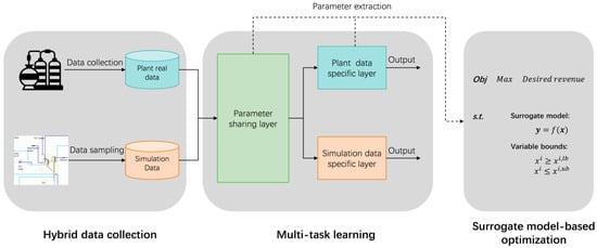
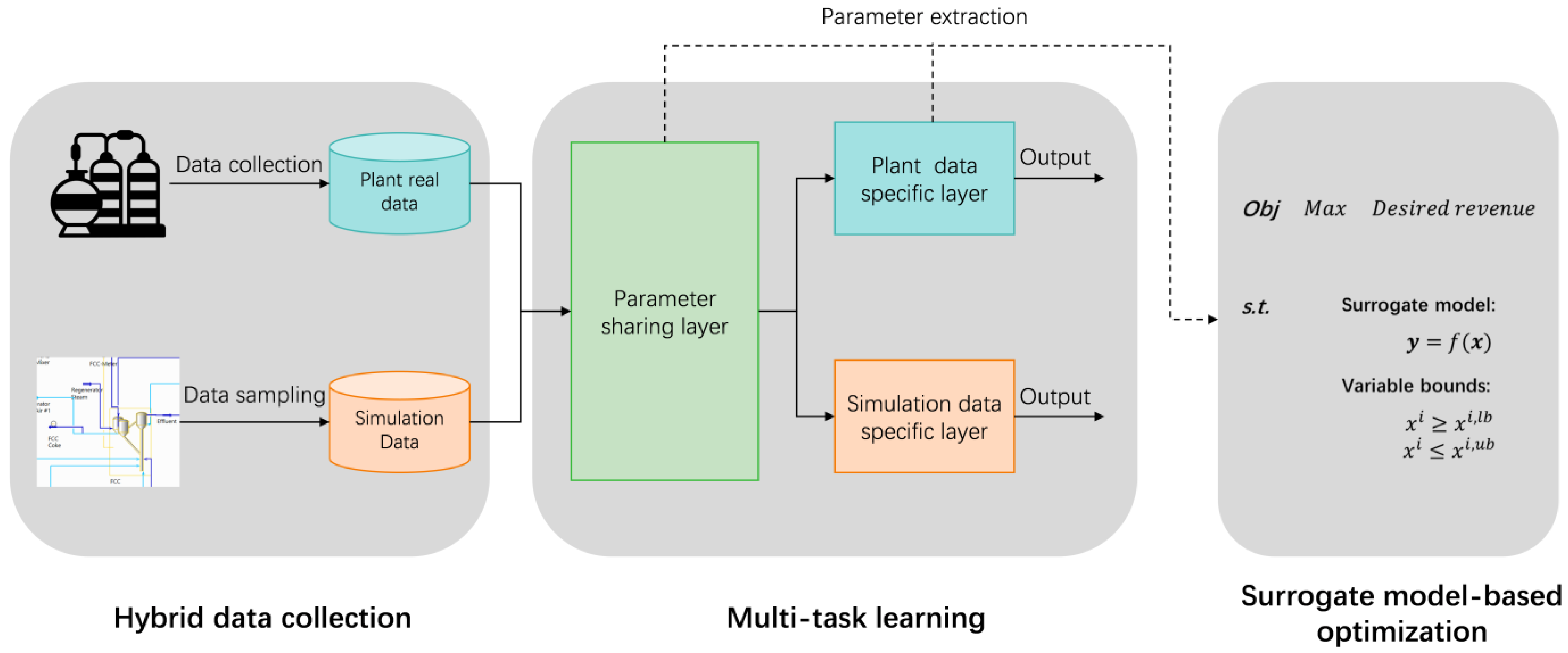
An integrated hybrid modeling and optimization framework is presented in Figure 1, consisting of three key modules: the hybrid data collection module, the multi-task learning prediction module, and the surrogate model-based optimization module. First, data from the plant and its simulation program are collected. Next, a multi-task learning model is trained on this hybrid dataset to predict product yields. Finally, the trained model is incorporated as a surrogate within an optimization framework to optimize the process’s operating conditions for higher economic performance. The following subsections provide detailed explanations of these modules.

Figure 1. Scheme of the integrated hybrid modelling and optimization framework.

2.1. Hybrid Data Collection

The relative importance of process input and output variables was established through iterative communication with on-site engineers, leveraging their operational knowledge. From dozens of candidate process variables, twelve key process inputs and five key yields were identified from the reactor–regenerator section, the main fractionator, and the gas plant. Additionally, two laboratory test results, x₁₃ and x₁₄, were included to capture fluctuations in feedstock properties. The sixth output variable y₆ represents the residue yield as a calculated mass balance term that represents coke formation and total substance loss.

The first step in gathering the dataset for modeling and optimization is selecting key process variables. The relative importance of process input and output variables was established through iterative communication with on-site engineers, leveraging their operational knowledge. From hundreds of candidate process variables, twelve key process inputs x₁ through x₁₂ and six key yields y₁ through y₆ were identified from the reactor–regenerator unit and subsequent separation units. Additionally, two feedstock oil property-related variables, x₁₃ and x₁₄, were included to capture fluctuations in feedstock properties. Density at 20 °C (x₁₃) is a fundamental property of petroleum fractions that indicates molecular composition. A higher density within a given boiling range correlates to lower alkane content in the feedstock, leading to higher proportions of cycloalkanes and aromatics in the products. Carbon residue content (x₁₄) quantifies the feedstock’s propensity for non-catalytic coke formation. The residue, primarily composed of condensed polycyclic aromatic hydrocarbons, serves as a precursor to coke deposits. Conradson carbon tests are carried out to predict direct catalyst deposition from feed components. The variables selected are listed in Table 1.

Table 1. Key process input and output variables of interest after variable selection.

Notation	Variable	Unit	Notation	Variable	Unit
x1	Reactor temperature	°C	y1	Dry gas yield	wt%
x2	Regenerator temperature	°C	y2	Liquefied gas yield	wt%
x3	Feed preheat temperature	°C	y3	Gasoline yield	wt%
x4	Feed flowrate	t/h	y4	Diesel yield	wt%
x5	Reflux flowrate	t/h	y5	Slurry oil yield	wt%
x6	Catalyst tank level	t	y6	Residue yield	wt%
x7	Fractionation tower cold reflux flow	t/h
x8	Light cycle oil extraction temperature	°C
x9	Fractionation tower bottom temperature	°C
x10	Supplemental absorbent flow rate	t/h
x11	Desorption tower top gas volume	Nm3/h
x12	Desorption tower top temperature	°C
x13	Mixed feedstock density (20 °C)	kg/cm3
x14	Mixed feedstock carbon residue content	wt%

After choosing the variables, a plant dataset was collected from the plant’s Distributed Control System (DCS), Manufacturing Execution System (MES), and Laboratory Information Management System (LIMS). The collected data span six months, containing two non-continuous three-month periods, March to May and July to September 2023. The variables of x₁ through x₁₂ and y₁ through y₆ were gathered from the DCS and MES, while x₁₃ and x₁₄ were extracted from LIMS record sheets.

To augment the plant dataset mentioned above, a simulation program has been built using Petro-SIM v7.3 (KBC Advanced Technologies Ltd., Walton-on-Thames, UK) [29], a commercial software developed by KBC Advanced Technologies. Petro-SIM comprises several sub-modules, including FCC-SIM for catalytic cracking, HCR-SIM for hydrocracking, and NHTR-SIM for catalytic reforming. FCC-SIM incorporates comprehensive feedstock characterization and detailed kinetic models of risers, reactors, and regenerators. It is extensively utilized for process design, operational optimization, and production planning.

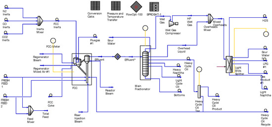
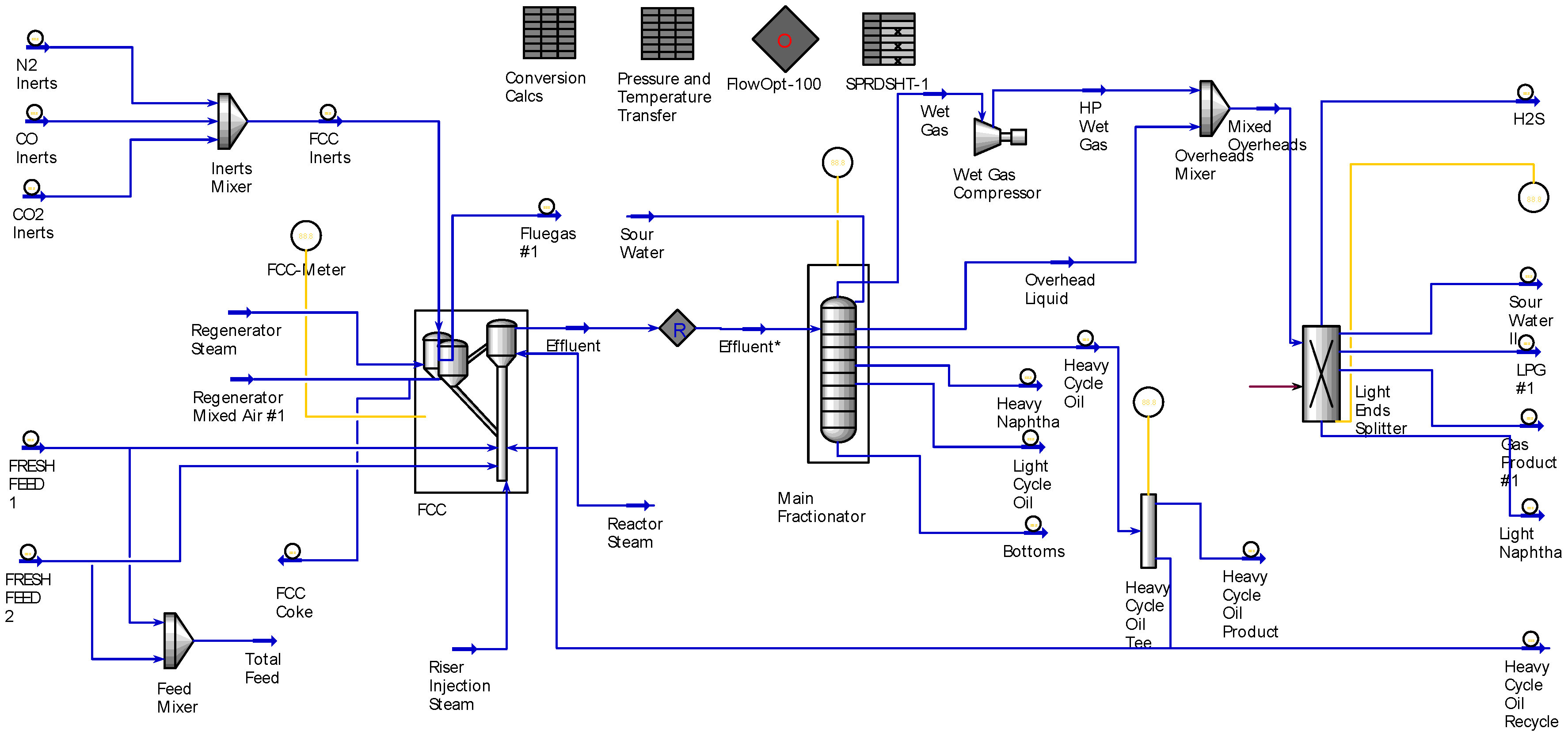
We first built an FCC-SIM model, with its process flow diagram (PFD) shown in Figure 2. We utilized the built-in ‘refinery-large’ component list, which includes 106 components such as hydrogen, carbon monoxide, and lighter hydrocarbons (C < 6). Additionally, hypothetical components were included based on the distillation curve at 10 °C intervals, ranging from 40 °C to 850 °C. The Peng–Robinson method was employed, as it is well-suited for property calculations in the FCC process. Then, operational data from the plant were used to calibrate this model. The overall feed masses and compositions were verified through mass balance criteria. After adjustments, these data were used in the calibration module to compute various parameters and calibration factors, such as reaction kinetics parameters.

Figure 2. Process flow diagram of the FCC process simulation in Petro-Sim.

After obtaining the model calibrated to plant data, we generated the simulation dataset through sampling across different operation conditions. A Python v3.10 script was developed to commute with the Component Object Model (COM) in Petro-SIM and automatically changed the key variables of reactor temperature, regenerator temperature, and feed preheat temperature in ranges defined in Table 2. To explore the ranges and possible combinations of input variables more effectively, the Latin Hypercube Sampling (LHS) [30] method was adopted.

Table 2. The operational variables and their corresponding adjustment range.

Variable	Unit	Lower Bound	Upper Bound
Reactor temperature	°C	505	528
Regenerator temperature	°C	668	685
Feed preheat temperature	°C	220	240

2.2. Multi-Task Learning Prediction Model

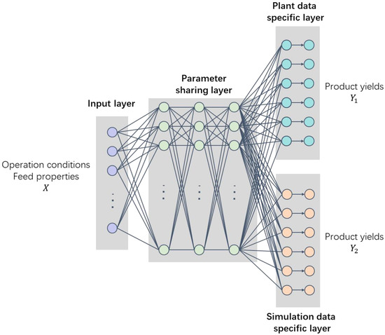
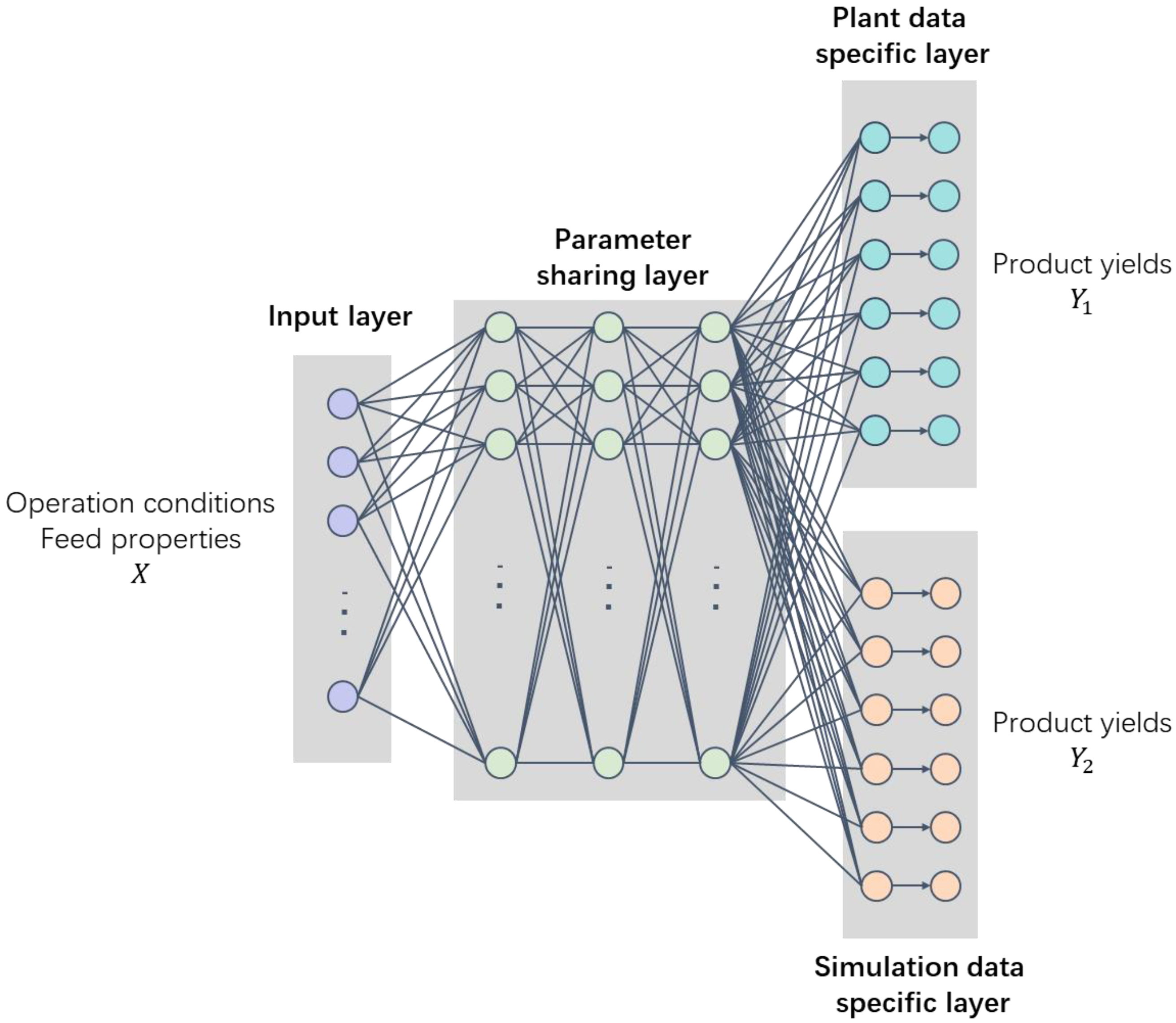
The hybrid dataset covers a broader range of operating conditions compared to the pure plant dataset, thus providing a solid foundation for modeling. To make the best use of these data and precisely capture the mapping relationship between the feedstock properties and operation conditions (inputs) and product yields (output), considering the different distribution ranges of the two datasets, a multi-task learning model was proposed, as shown in Figure 3. The model is a deep neural network with two components: the parameter-sharing backbone and the task-specific heads.

Figure 3. Structure of the multi-task learning model.

The parameter-sharing backbone has three layers of neurons that extract features common to hybrid inputs. The forward computation of these fully connected layers is shown in Equations (1) and (2).

$${\mathit{a}}^0=\mathit{x}$$

(1)

$${\mathit{z}}^l={\mathit{W}}^l{\mathit{a}}^{l-1}+{\mathit{b}}^l, l=1,2,3$$

(2)

where ${\mathit{W}}^l\in {\mathbb{R}}^{m_l\times m_{l-1}}$ is the weight matrix of the l-th layer, $m_l$ is the number of neurons in the l-th layer, ${\mathit{a}}^{l-1}\in {\mathbb{R}}^{m_{l-1}}$ is the activation vector (i.e., output) of the l-1-th layer, ${\mathit{b}}^l\in {\mathbb{R}}^{m_l}$ is the bias vector of the l-th layer, and ${\mathit{z}}^l$ is the linear combination result for the l-1-th layer neurons.

$${\mathit{a}}^l=\sigma \left({\mathit{z}}^l\right), l=1,2,3$$

(3)

where $\sigma (·)$ is the activation function, applied element-wise to the vector ${\mathit{z}}^l$ (Equation (3)). Here, SiLU is used as the activation function, which is continuous and differentiable, as shown in Equation (4).

$$SiLU\left({\mathit{z}}^l\right)={\mathit{z}}^l·{\displaystyle \frac{1}{1+e^{-{\mathit{z}}^l}}}$$

(4)

where after feature extraction, the task-specific part adopts specific output layers to predict the outputs for the plant data and simulation data, respectively, as expressed in Equations (5) and (6).

$${\mathit{z}}_1^L={\mathit{W}}^{L_1}{\mathit{a}}^{L-1}+{\mathit{b}}^{L_1}$$

(5)

$${\mathit{z}}_2^L={\mathit{W}}^{L_2}{\mathit{a}}^{L-1}+{\mathit{b}}^{L_2}$$

(6)

Finally, a SoftMax layer is added to normalize the output and compute the final prediction for the desired product yields, as shown in Equation (7).

$${\mathit{y}}_1,{\mathit{y}}_2=SoftMax({\mathit{z}}_1^L,{\mathit{z}}_2^L)$$

(7)

During training, the loss function is designed as the weighted sum of mean squared error (MSE) loss for the prediction of ${\mathit{y}}_1$ and ${\mathit{y}}_2$, as shown in Equation (8).

$$Loss=\sum _i{\displaystyle \frac{1}{N_1}}{\left({\mathit{y}}_1-\widehat{{\mathit{y}}_1}\right)}^2+\lambda \sum _j{\displaystyle \frac{1}{N_2}}{\left({\mathit{y}}_2-\widehat{{\mathit{y}}_2}\right)}^2$$

(8)

where ${\mathit{y}}_1,{\mathit{y}}_2$ are the prediction values, $\widehat{{\mathit{y}}_1},\widehat{{\mathit{y}}_2}$ are the true values, $N_1,N_2$ are the batch sizes for the two training datasets and $\lambda$ is the weight to balance the learning performance of the prediction task for plant data and simulation data.

Before training, the plant and simulation datasets were divided into training, validation, and test sets in a 7:2:1 ratio. During the training phase, the batch size for the plant data and the simulation data was set proportionally according to the size of each dataset to ensure that the number of batches was the same.

2.3. Surrogate Model-Based Optimization Model

The trained multi-task prediction model is regarded as a surrogate model and represents the input–output mappings of the FCC process. With this model, we formulated a non-linear programming (NLP) optimization model for the FCC process.

The objective is to maximize the revenue from the desired product output (i.e., LNG, gasoline, diesel) per unit of feedstock oil, as expressed in Equation (9).

$$\mathit{M}\mathit{a}\mathit{x} obj={\displaystyle \frac{{x_4(P}_1{y}_1+P_2{y}_2+P_3{y}_3)}{100}}$$

(9)

where $P_1, { P}_2, P_3$ are the prices of LNG, gasoline, and diesel, and are set at 5000, 9000, and 8000 CNY/t. The trained weight matrices of ${\mathit{W}}^1,{\mathit{W}}^2,{\mathit{W}}^3,{\mathit{W}}^{L_1}$ and biases of ${\mathit{b}}^1,{\mathit{b}}^2,{\mathit{b}}^3,{\mathit{b}}^{L_1}$ are extracted from the prediction model and the explicit form of the neural network is embedded as equality constraints in the optimization model, as shown in Equations (10)–(13).

$$h_{j_1}^1={\displaystyle \frac{{\sum }_i{(W}_{i,j_1}^1{x}_i+b_{j_1}^1)}{1+e^{-{\sum }_i(W_{i,j_1}^1{x}_i+b_{j_1}^1)}}}$$

(10)

$$h_{j_2}^2={\displaystyle \frac{{\sum }_{j_1}(W_{j_1,j_2}^2{h}_{j_1}^1+b_{j_2}^2)}{1+e^{-{\sum }_{j_1}(W_{j_1,j_2}^2{h}_{j_1}^1+b_{j_2}^2)}}}$$

(11)

$$h_{j_3}^3={\displaystyle \frac{{\sum }_{j_2}(W_{j_2,j_3}^2{h}_{j_2}^2+b_{j_3}^3)}{1+e^{-{\sum }_{j_2}(W_{j_2,j_3}^2{h}_{j_2}^2+b_{j_3}^3)}}}$$

(12)

$$y_k=100\ast SoftMax\left(\sum _{j_3}{W}_{j_3,k}^{L_1}{h}_{j_3}^3+b_{j_4}^{L_1}\right)$$

(13)

where $i$ is the index of input, $j_1, j_2, { j}_3$ are the indices of the neurons in the hidden layers (set to 256) and $k$ is the index of the output.

The optimization variables are reactor temperature (x₁), regenerator temperature (x₂), and preheat temperature (x₃), all of which are constrained by respective upper bounds and lower bounds, as shown in Equations (14) and (15).

$$x_1, x_2,x_3\ge x_1^{lo}, x_2^{lo},x_3^{lo}$$

(14)

$$x_1, x_2,x_3\le x_1^{up},x_2^{up},x_3^{up}$$

(15)

For on-site operational optimization, it is important to ensure operational continuity and consider integration with advanced process control (APC) systems by keeping the optimization space manageable. After discussions with plant operators, we selected an optimization range of ±5 °C for both reactor temperature and feed preheat temperature, and ±3 °C for regenerator temperature. The optimization program is implemented in GAMS v38.2 on an Intel Core i7-9700CPU @ 3.00 GHz CPU with 16.0 GB RAM and optimized by the IPOPT [31] solver.

3. Results

3.1. Plant and Simulation Dataset Distribution

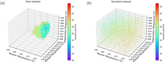
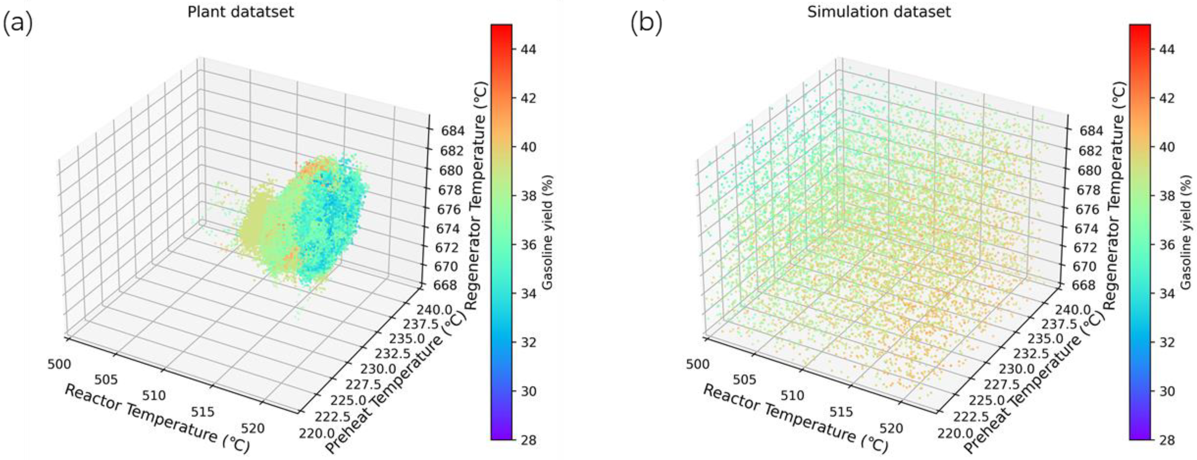
Following the methodology outlined in Section 2.1, a hybrid dataset was created, consisting of a plant dataset with 264,964 records spanning March to May and July to September 2023, along with a simulation dataset of 8760 records. Although the plant dataset is large, its coverage in the space spanned by key independent variables is limited. As shown in Figure 4, we present the distribution of the plant and simulation datasets across three variable dimensions. It can be observed that the plant dataset is concentrated in the central region of the cube. In contrast, the simulation dataset, sampled from the simulation program, nearly covers the entire area of the cube.

Figure 4. Data distribution of the (a) plant dataset and (b) simulation dataset.

3.2. Baseline Pure Data-Driven Model Prediction Results

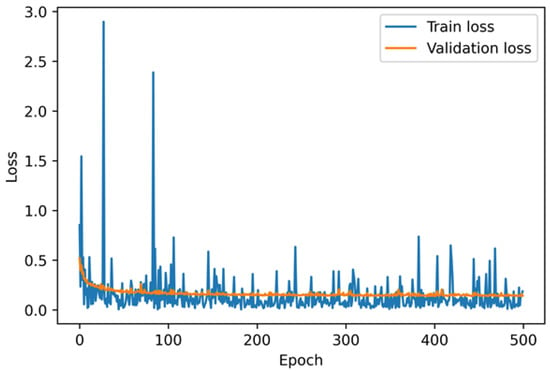
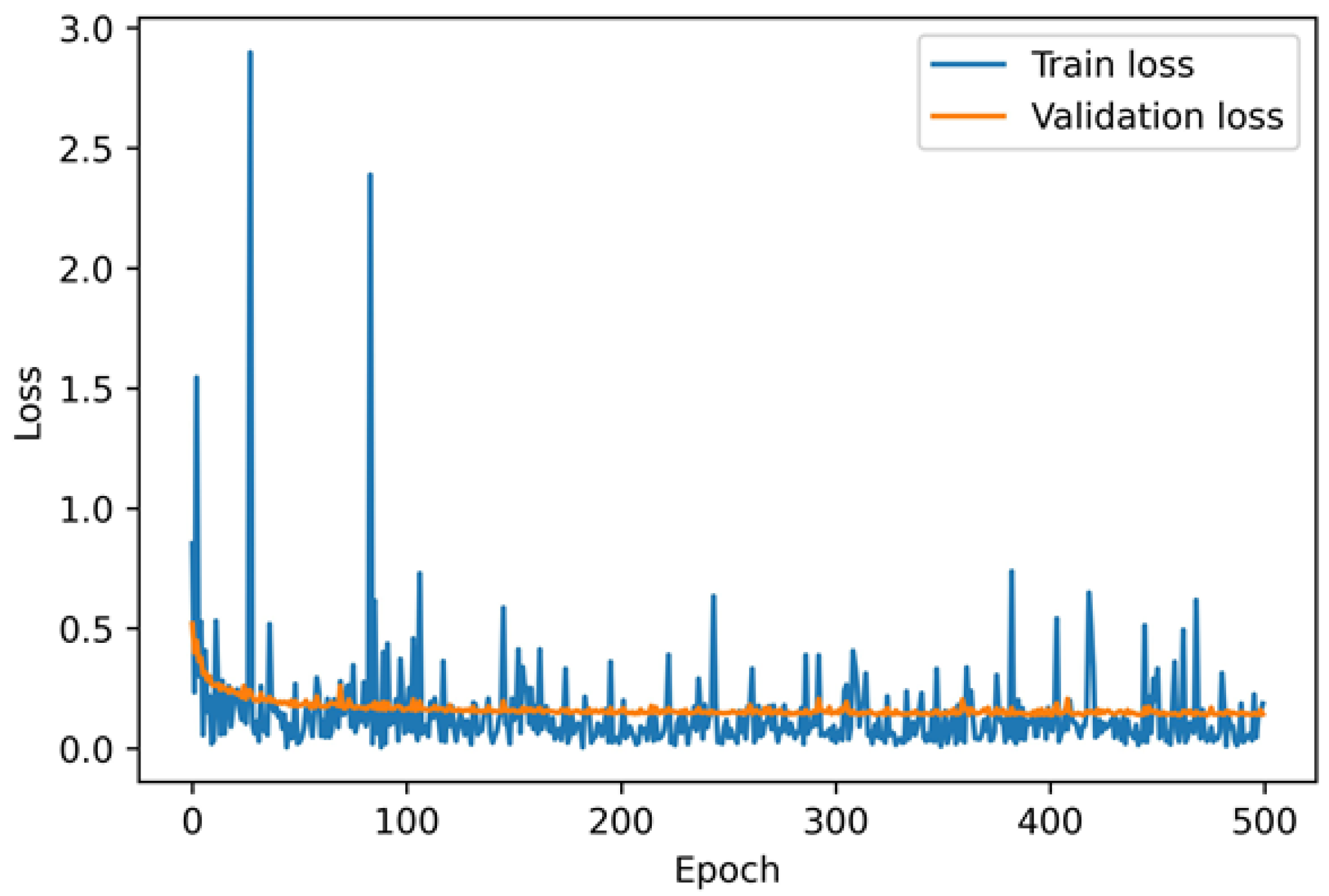
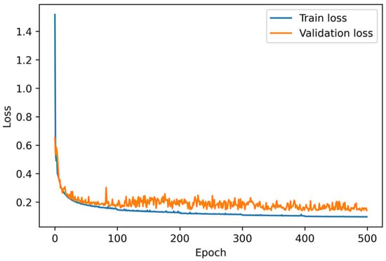
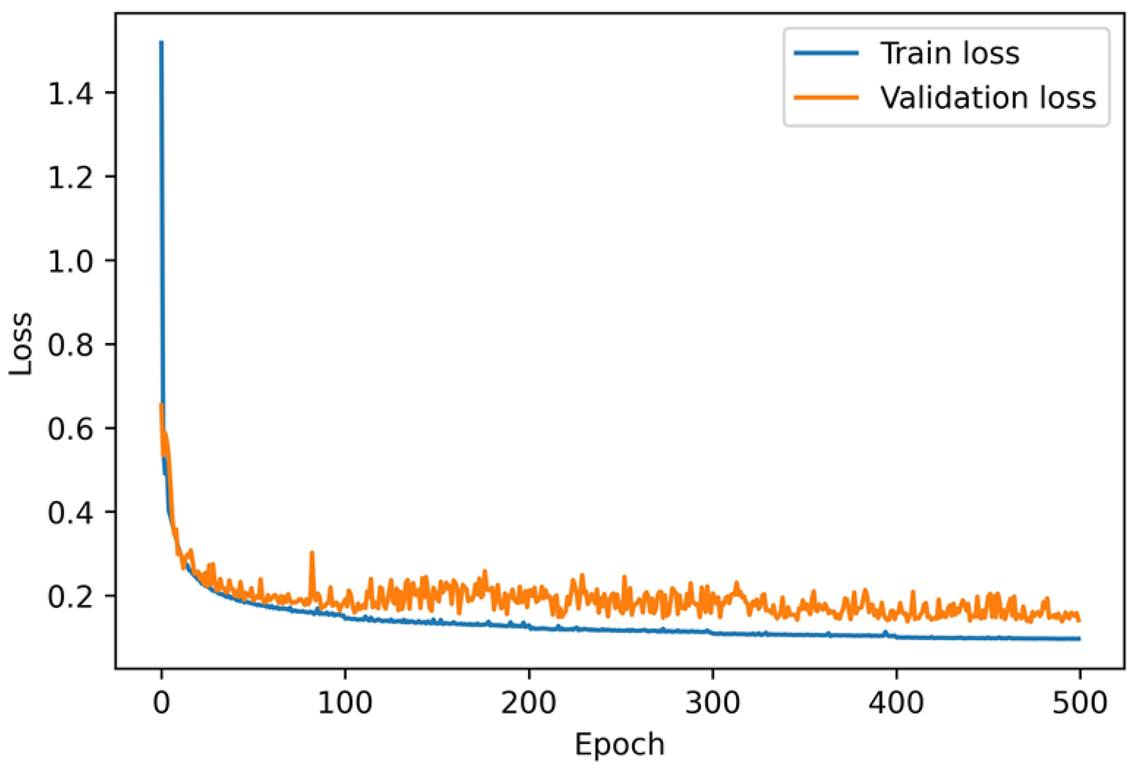
As a baseline comparison, we adopt a pure data-driven model obtained using the plant dataset to train a deep neural network with three layers of hidden neurons. The input layer is $x_1$ to $x_{14}$ and the output is $y_1$ to $y_6$ as defined in Table 1. The activation function is SiLU, and a SoftMax layer is added before the output. Figure 5 illustrates the trend of the loss function during the training process. As shown in the figure, although the loss continues to decrease, the training loss curve exhibits several sharp spikes, indicating instability in the training process and suggesting a risk of overfitting. The model is trained for 500 epochs.

Figure 5. Train and validation loss of the pure data-driven model.

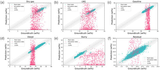
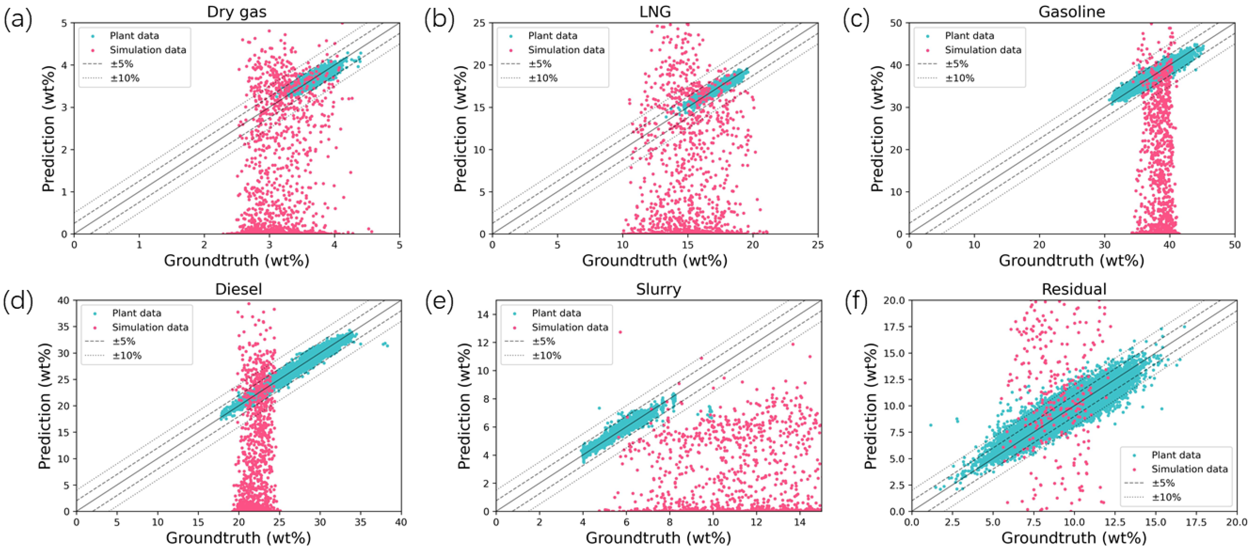
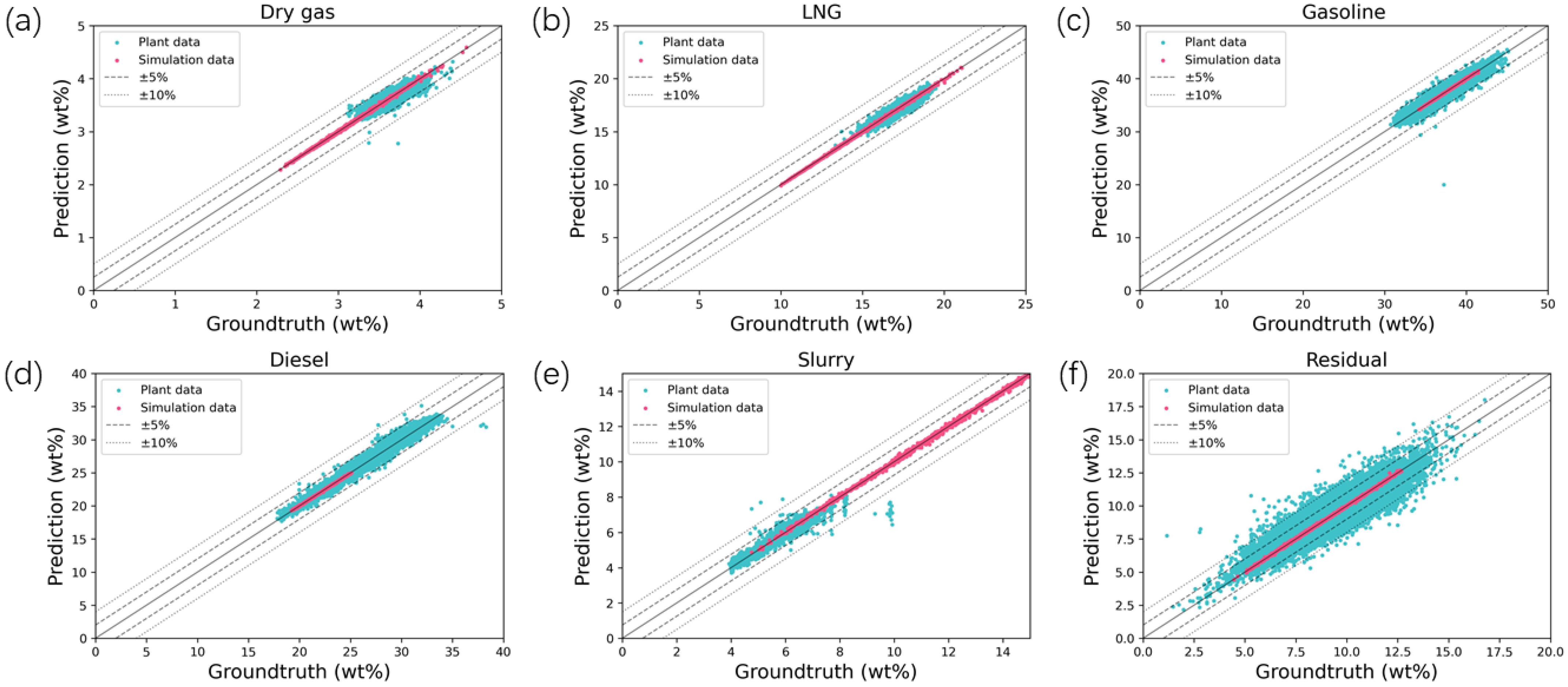
After training, the model is used to predict the product yields on both the test plant dataset and the simulation dataset, with the results shown in Figure 6. As illustrated, the model performs well on the plant dataset (cyan dots), with prediction points closely aligning with the diagonal line, and most predictions falling within ±10% of the actual data. However, the model’s performance deteriorates significantly on the simulation dataset (pink dots), where the predictions are highly inaccurate.

Figure 6. Prediction results of the pure data-driven model on the test datasets for (a) dry gas, (b) LNG, (c) gasoline, (d) diesel, (e) slurry, and (f) residual.

Table 3 demonstrates metrics comparisons of the prediction performance of this model on the plant dataset and simulation dataset. The purely data-driven model achieves high prediction accuracy on the plant dataset, with MSE ranging from 0.0029 to 0.3712 and mean absolute percentage error (MAPE) between 0.82% and 4.90%. However, on the simulation dataset, the predictions become highly inaccurate, with MSE reaching 6.3814 to 5413.0770 and MAPE soaring to 72.11% to 715.72%, indicating a failure in prediction on the simulation dataset.

Table 3. Prediction precision results of the pure data-driven model.

Yield (wt%)	Plant Dataset		Simulation Dataset
	MSE	MAPE	MSE	MAPE
Dry gas	0.0029	1.15%	6.3814	72.11%
LNG	0.0337	0.82%	173.6118	78.71%
Gasoline	0.2757	1.08%	1073.6084	78.17%
Diesel	0.1372	1.02%	383.3285	78.65%
Slurry	0.0139	1.37%	128.6065	85.34%
Residual	0.3712	4.90%	5413.0770	715.72%

This phenomenon is because the purely data-driven model was trained solely on the plant dataset, which, as revealed earlier in Figure 4, has limited coverage of the independent variable space. Consequently, when this model is used to predict points in the simulation dataset that fall outside its data distribution range, it results in extrapolation failure.

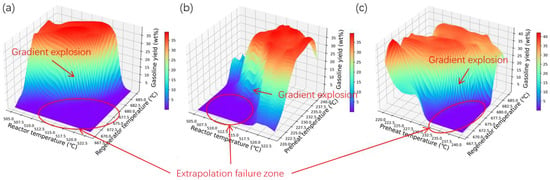
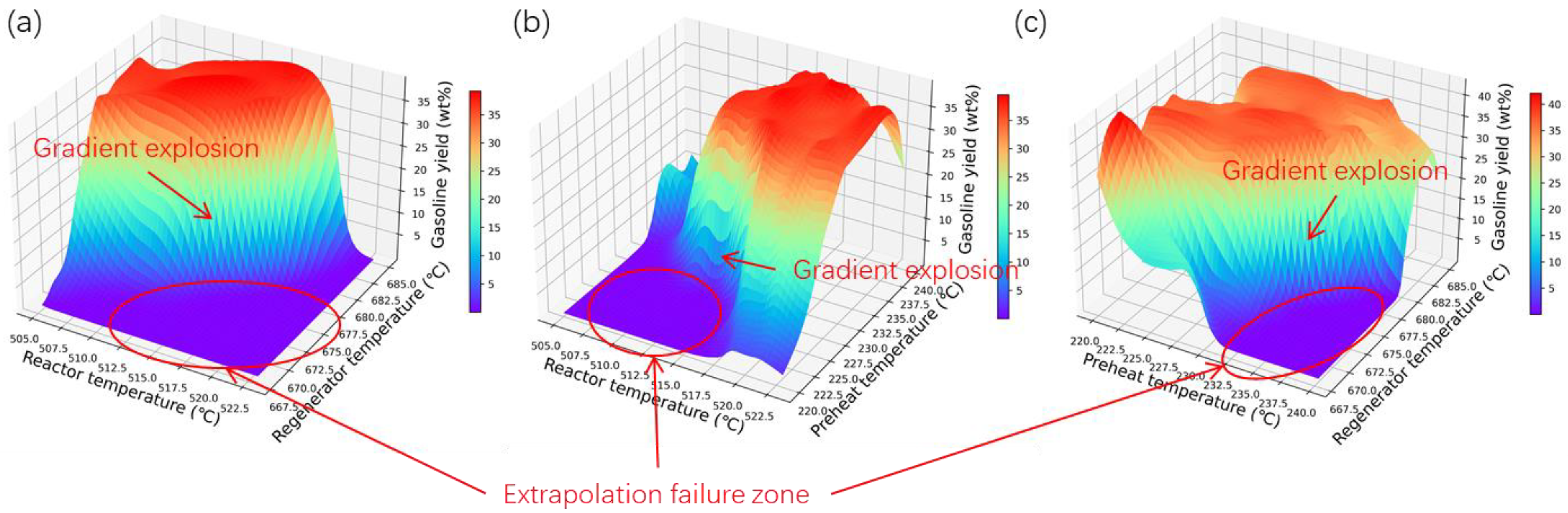
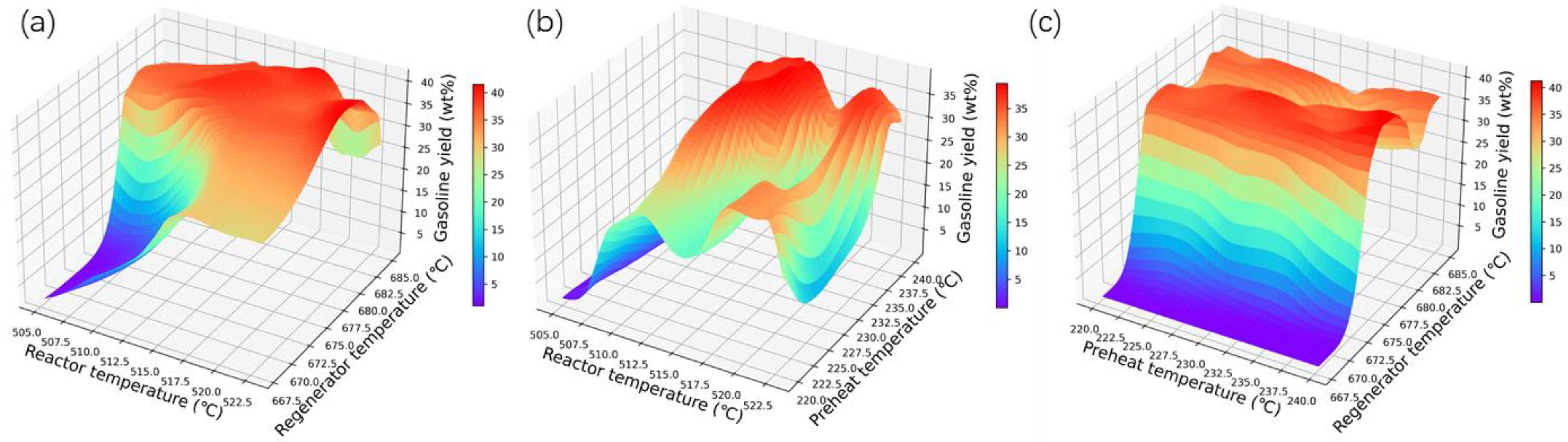
The phenomenon of extrapolation failure can be further elucidated through trend surface analysis of the dependent variable with respect to the independent variables. Figure 7 displays the trend surface of gasoline yield as it varies with the three independent variables of reactor temperature, regenerator temperature, and feed preheat temperature at the first data point of the plant dataset. There are areas on the surface where the gasoline yield is 0, indicating regions not covered by the data distribution during the model training process. In these areas, extrapolation failure occurs, and gradient explosion phenomena can be observed in the positions adjacent to these regions. If this model is used for optimization, it would also present insurmountable challenges for the optimization solution.

Figure 7. Trend surface of gasoline yield with respect to (a) reactor temperature and regenerator temperature, (b) reactor temperature and preheat temperature, and (c) regenerator temperature and preheat temperature in the pure data-driven model.

3.3. Multi-Task Model Prediction Results

A multi-task learning model proposed in Section 2.2 was trained using both the plant and the simulated dataset. The loss function curve during training is shown in Figure 8. As shown in the figure, unlike the pure data-driven model, the loss function decreases steadily as the training progresses. After 500 epochs, the loss functions for both the training and validation sets have converged.

Figure 8. Train and validation loss of the multi-task learning model.

After training, the multi-task learning model is tested on the plant and simulation dataset, and the prediction results are shown in Figure 9. For all the product yields, the prediction results are around the diagonal lines for the plant and simulation datasets, suggesting satisfactory performances on both datasets.

Figure 9. Prediction results of the multi-task learning model on the test datasets for (a) dry gas, (b) LNG, (c) gasoline, (d) diesel, (e) slurry, and (f) residual.

Table 4 provides a detailed breakdown of the MSE and MAPE for the prediction results. For the plant dataset, the MSE for product yields ranges from 0.0032 to 0.3621, with MAPE between 0.98% and 4.84%. For the simulation dataset, the MSE ranges from 0.0002 to 0.0055, and MAPE from 0.09% to 0.47%. These results indicate that the multi-task learning model performs well on both the plant and simulation dataset prediction tasks.

Table 4. Prediction precision results of the multi-task learning model.

Yield (wt%)	Plant Dataset		Simulation Dataset
	MSE	MAPE	MSE	MAPE
Dry gas	0.0032	1.20%	0.0002	0.31%
LNG	0.0311	0.78%	0.0028	0.27%
Gasoline	0.2695	1.05%	0.0020	0.09%
Diesel	0.1297	0.98%	0.0015	0.13%
Slurry	0.0148	1.45%	0.0055	0.47%
Residual	0.3621	4.84%	0.0019	0.36%

Further analysis of the multi-task learning model revealed that the trend surface for gasoline yield concerning the three independent variables no longer exhibited regions of extrapolation failure, as shown in Figure 10. Additionally, the surface did not present characteristics detrimental to the optimization process, such as vanishing gradients. Therefore, this model is suitable for use as a surrogate model embedded within an optimization framework to enhance operational procedures.

Figure 10. Trend surface of gasoline yield with respect to (a) reactor temperature and regenerator temperature, (b) reactor temperature and preheat temperature, and (c) regenerator temperature and preheat temperature in the multi-task learning model.

3.4. Optimization Results

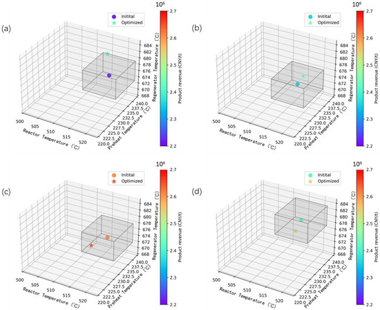
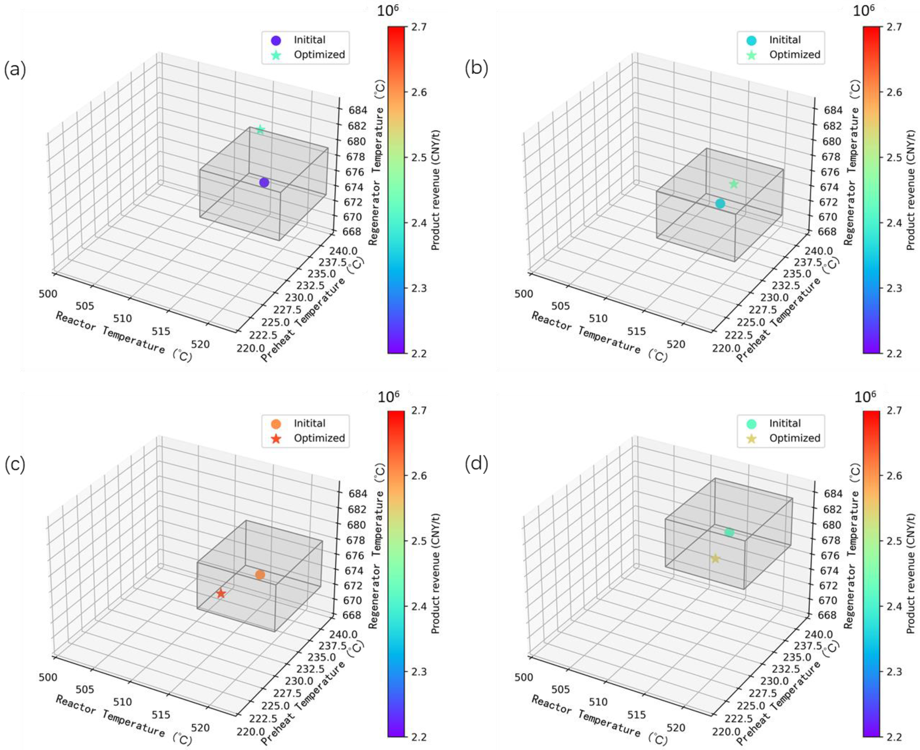
Using the trained multi-task learning model parameters, an optimization model is constructed for the operational optimization of the FCC unit. A batch of 300 points from the dataset is sampled and run through the optimization model. Figure 11 presents the optimization results for four specific points, corresponding to the data for 26 March 2023, 17 April 2023, 6 May 2023, and 19 July 2023. As depicted in the figure, the optimization is centered on the plant’s operational point, with the search space defined as a cube across three optimization variables: reaction temperature, regeneration temperature, and feed preheat temperature, each varying by ±5 °C, ±5 °C, and ±3 °C, respectively. The initial points are represented by circles, while the optimized points are indicated by stars. After optimization, the product revenues for the four points increased significantly.

Figure 11. Optimization results demonstration of (a) 26 March 2023, (b) 17 April 2023, (c) 6 May 2023, and (d) 19 July 2023.

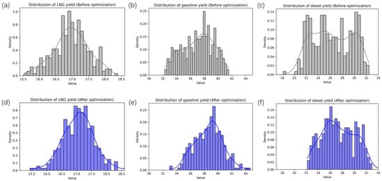
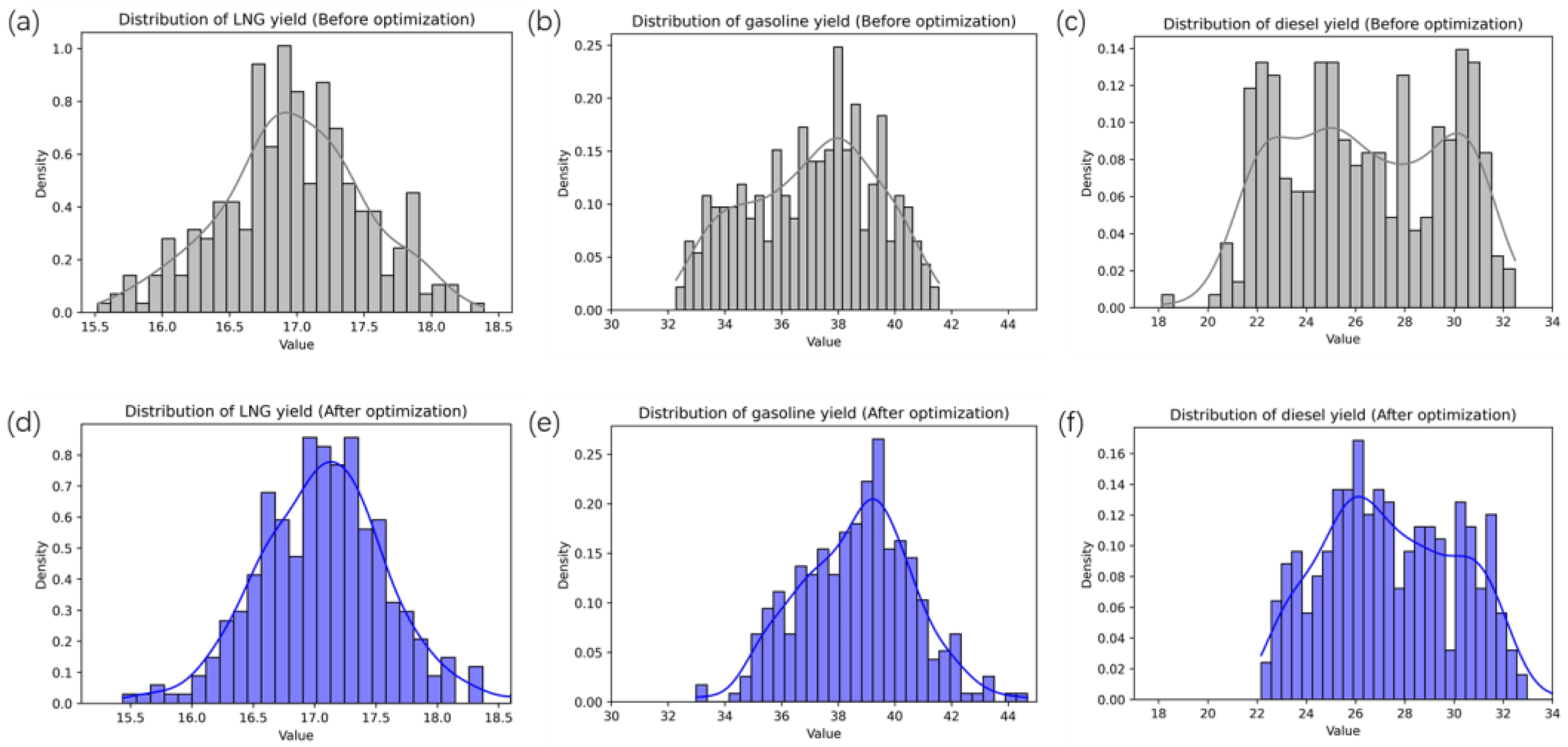
Figure 12 presents the yield distribution of the desired products (i.e., LNG, gasoline, diesel) before and after optimization in histograms and Kernel Density Estimation (KDE) plots for all 300 points. In the figure, the gray bars and curves represent the results before optimization, while the blue bars and curves represent the results after optimization. It can be observed from the figure that, after optimization, the bars corresponding to higher yields for LNG, gasoline, and diesel have increased in the yield distribution histograms. Additionally, the peaks of the probability density curves have shifted towards higher yields, indicating that the optimization has improved the yields of these desired products.

Figure 12. Product distribution of (a,d) LNG, (b,e) gasoline, and (c,f) diesel before and after optimization.

Table 5 provides a detailed overview of the optimization results for these 300 points. On average, the yield of LNG increased from 16.97 wt% to 17.07 wt%, the yield of gasoline from 37.06 wt% to 38.64 wt%, and the yield of diesel from 26.36 wt% to 27.41 wt%. Consequently, the product revenue, reflecting this improvement, increased from CNY 2,413,730 to CNY 2,502,356 per hour, representing a 3.7% increase. This illustrates the substantial potential of the optimization model for enhancing the economic performance of the FCC unit through adjustments in operational variables.

Table 5. Comparison of product yields and product revenues before and after optimization.

	Before Optimization	After Optimization	Relative Change
Average LNG yield	16.97 wt%	17.07 wt%	+0.59%
Average gasoline yield	37.06 wt%	38.64 wt%	+4.26%
Average diesel yield	26.36 wt%	27.41 wt%	+3.98%
Average product revenue	2,413,730 CNY/h	2,502,356 CNY/h	+3.67%

In practice, obtaining data from a plant that covers multiple operating conditions is often challenging. While there is an abundance of data available from the plant, most of the data are steady-state data with limited informational content. Therefore, relying solely on the available plant data for purely data-driven modeling is unreliable. This is why we introduce simulated data generated from mechanistic models for hybrid modeling. However, the accuracy of such hybrid models still largely depends on the quality of the dataset. When the plant uses new feedstock with properties significantly different from those in the dataset or operates under new conditions, the performance of the hybrid model may deteriorate significantly. In such cases, it is necessary to retrain the model using newly collected data to maintain its accuracy.

4. Conclusions

In this work, we address the operational optimization of the FCC process in an industrial setting by proposing an integrated framework that combines mechanistic and data-driven modeling with optimization. This framework involves using a simulation program to augment plant data samples collected from the field and applying a multi-task learning model to train the prediction model. This approach achieved product yield predictions with errors of less than 4.84% for the plant dataset and less than 0.47% for the simulation dataset. The trained multi-task learning model was then embedded as a surrogate model within the optimization framework to optimize operational variables. Testing with 300 points demonstrated that this framework could improve LNG, gasoline, and diesel yields by an average of 0.10 wt%, 1.58 wt%, and 1.05 wt%, respectively, and increase final product revenue by 3.67%. This illustrates the substantial potential of this framework for enhancing the economic benefits of industrial FCC processes.

References

- Pinheiro, C.I.C.; Fernandes, J.L.; Domingues, L.; Chambel, A.J.S.; Graça, I.; Oliveira, N.M.C.; Cerqueira, H.S.; Ribeiro, F.R. Fluid Catalytic Cracking (FCC) Process Modeling, Simulation, and Control. Ind. Eng. Chem. Res. 2011, 51, 1–29. [Google Scholar] [CrossRef] [Scilit]
- Xie, Y.; Zhang, Y.; He, L.; Jia, C.Q.; Yao, Q.; Sun, M.; Ma, X. Anti-deactivation of zeolite catalysts for residue fluid catalytic cracking. Appl. Catal. A Gen. 2023, 657, 119159. [Google Scholar] [CrossRef] [Scilit]
- Palos, R.; Gutiérrez, A.; Fernández, M.L.; Azkoiti, M.J.; Bilbao, J.; Arandes, J.M. Converting the Surplus of Low-Quality Naphtha into More Valuable Products by Feeding It to a Fluid Catalytic Cracking Unit. Ind. Eng. Chem. Res. 2020, 59, 16868–16875. [Google Scholar] [CrossRef] [Scilit]
- Gholami, Z.; Gholami, F.; Tišler, Z.; Tomas, M.; Vakili, M. A Review on Production of Light Olefins via Fluid Catalytic Cracking. Energies 2021, 14, 1089. [Google Scholar] [CrossRef] [Scilit]
- Chen, Q.; Ding, J.; Chai, T.; Pan, Q. Evolutionary Optimization Under Uncertainty: The Strategies to Handle Varied Constraints for Fluid Catalytic Cracking Operation. IEEE Trans. Cybern. 2020, 52, 2249–2262. [Google Scholar] [CrossRef] [Scilit] [PubMed]
- Sildir, H.; Arkun, Y.; Canan, U.; Celebi, S.; Karani, U.; Er, I. Dynamic modeling and optimization of an industrial fluid catalytic cracker. J. Process Control 2015, 31, 30–44. [Google Scholar] [CrossRef] [Scilit]
- Lopes, G.; Rosa, L.; Mori, M.; Nunhez, J.; Martignoni, W. Three-dimensional modeling of fluid catalytic cracking industrial riser flow and reactions. Comput. Chem. Eng. 2011, 35, 2159–2168. [Google Scholar] [CrossRef] [Scilit]
- Zhang, Y.; Liu, M.; Zhao, L.; Liu, S.; Gao, J.; Xu, C.; Ma, M.; Meng, Q. Modeling, simulation, and optimization for producing ultra-low sulfur and high-octane number gasoline by separation and conversion of fluid catalytic cracking naphtha. Fuel 2021, 299, 120740. [Google Scholar] [CrossRef] [Scilit]
- Long, J.; Mao, M.S.; Zhao, G.Y. Model Optimization for an Industrial Fluid Catalytic Cracking Riser-regenerator Unit by Differential Evolution Algorithm. Pet. Sci. Technol. 2015, 33, 1380–1387. [Google Scholar] [CrossRef] [Scilit]
- He, G.; Zhou, C.; Luo, T.; Zhou, L.; Dai, Y.; Dang, Y.; Ji, X. Online Optimization of Fluid Catalytic Cracking Process via a Hybrid Model Based on Simplified Structure-Oriented Lumping and Case-Based Reasoning. Ind. Eng. Chem. Res. 2021, 60, 412–424. [Google Scholar] [CrossRef] [Scilit]
- Zhao, X.; Sun, S. Lumped Kinetic Modeling Method for Fluid Catalytic Cracking. Chem. Eng. Technol. 2020, 43, 2493–2500. [Google Scholar] [CrossRef] [Scilit]
- Weekman, V.W.; Nace, D.M. Kinetics of catalytic cracking selectivity in fixed, moving, and fluid bed reactors. AIChE J. 1970, 16, 397–404. [Google Scholar] [CrossRef] [Scilit]
- Weekman, V.W. Model of Catalytic Cracking Conversion in Fixed, Moving, and Fluid-Bed Reactors. Ind. Eng. Chem. Process Des. Dev. 1968, 7, 90–95. [Google Scholar] [CrossRef] [Scilit]
- Arbel, A.; Huang, Z.; Rinard, I.H.; Shinnar, R.; Sapre, A.V. Dynamic and Control of Fluidized Catalytic Crackers. 1. Modeling of the Current Generation of FCC’s. Ind. Eng. Chem. Res. 1995, 34, 1228–1243. [Google Scholar] [CrossRef] [Scilit]
- Ebrahimi, A.A.; Mousavi, H.; Bayesteh, H.; Towfighi, J. Nine-lumped kinetic model for VGO catalytic cracking; using catalyst deactivation. Fuel 2018, 231, 118–125. [Google Scholar] [CrossRef] [Scilit]
- Yang, B.; Zhou, X.; Chen, C.; Yuan, J.; Wang, L. Molecule Simulation for the Secondary Reactions of Fluid Catalytic Cracking Gasoline by the Method of Structure Oriented Lumping Combined with Monte Carlo. Ind. Eng. Chem. Res. 2008, 47, 4648–4657. [Google Scholar] [CrossRef] [Scilit]
- John, Y.M.; Mustafa, M.A.; Patel, R.; Mujtaba, I.M. Parameter estimation of a six-lump kinetic model of an industrial fluid catalytic cracking unit. Fuel 2019, 235, 1436–1454. [Google Scholar] [CrossRef] [Scilit]
- Lee, J.H.; Kang, S.; Kim, Y.; Park, S. New Approach for Kinetic Modeling of Catalytic Cracking of Paraffinic Naphtha. Ind. Eng. Chem. Res. 2011, 50, 4264–4279. [Google Scholar] [CrossRef] [Scilit]
- Yang, S.; Wang, N. A P systems based hybrid optimization algorithm for parameter estimation of FCCU reactor–regenerator model. Chem. Eng. J. 2012, 211–212, 508–518. [Google Scholar] [CrossRef] [Scilit]
- Du, Y.; Sun, L.; Berrouk, A.S.; Zhang, C.; Chen, X.; Fang, D.; Ren, W. Novel Integrated Reactor-Regenerator Model for the Fluidized Catalytic Cracking Unit Based on an Equivalent Reactor Network. Energy Fuels 2019, 33, 7265–7275. [Google Scholar] [CrossRef] [Scilit]
- Palos, R.; Rodríguez, E.; Gutiérrez, A.; Bilbao, J.; Arandes, J.M. Kinetic modeling for the catalytic cracking of tires pyrolysis oil. Fuel 2022, 309, 122055. [Google Scholar] [CrossRef] [Scilit]
- Nazarova, G.; Ivashkina, E.; Ivanchina, E.; Oreshina, A.; Vymyatnin, E. A predictive model of catalytic cracking: Feedstock-induced changes in gasoline and gas composition. Fuel Process. Technol. 2021, 217, 106720. [Google Scholar] [CrossRef] [Scilit]
- Qin, X.; Ye, L.; Liu, J.; Xu, Y.; Murad, A.; Ying, Q.; Shen, H.; Wang, X.; Hou, L.; Pu, X.; et al. A molecular-level coupling model of fluid catalytic cracking and hydrotreating processes to improve gasoline quality. Chem. Eng. J. 2023, 451, 138778. [Google Scholar] [CrossRef] [Scilit]
- Chen, Z.; Feng, S.; Zhang, L.; Wang, G.; Shi, Q.; Xu, Z.; Zhao, S.; Xu, C. Molecular-level kinetic modeling of heavy oil fluid catalytic cracking process based on hybrid structural unit and bond-electron matrix. AIChE J. 2021, 67, e17027. [Google Scholar] [CrossRef] [Scilit]
- Chen, C.; Zhou, L.; Ji, X.; He, G.; Dai, Y.; Dang, Y. Adaptive Modeling Strategy Integrating Feature Selection and Random Forest for Fluid Catalytic Cracking Processes. Ind. Eng. Chem. Res. 2020, 59, 11265–11274. [Google Scholar] [CrossRef] [Scilit]
- Long, J.; Li, T.; Yang, M.-L.; Hu, G.; Zhong, W. Hybrid Strategy Integrating Variable Selection and a Neural Network for Fluid Catalytic Cracking Modeling. Ind. Eng. Chem. Res. 2019, 58, 247–258. [Google Scholar] [CrossRef] [Scilit]
- Tian, W.; Wang, S.; Sun, S.; Li, C.; Lin, Y. Intelligent prediction and early warning of abnormal conditions for fluid catalytic cracking process. Chem. Eng. Res. Des. 2022, 181, 304–320. [Google Scholar] [CrossRef] [Scilit]
- Yang, F.; Dai, C.; Tang, J.; Xuan, J.; Cao, J. A hybrid deep learning and mechanistic kinetics model for the prediction of fluid catalytic cracking performance. Chem. Eng. Res. Des. 2020, 155, 202–210. [Google Scholar] [CrossRef] [Scilit]
- Li, X.; Zhang, L.; Sun, Y.; Jiang, B.; Zhang, R.; Li, X.; Yang, N. Investigation on steam injection condition in refining vacuum furnace. Chem. Eng. Sci. 2015, 135, 509–516. [Google Scholar] [CrossRef] [Scilit]
- Loh, W.-L. On Latin hypercube sampling. Ann. Stat. 1996, 24, 2058–2080. [Google Scholar] [CrossRef] [Scilit]
- Andrei, N. Continuous Nonlinear Optimization for Engineering Applications in Gams Technology; Springer Science+Business Media: New York, NY, USA, 2017. [Google Scholar]
Disclaimer/Publisher’s Note: The statements, opinions and data contained in all publications are solely those of the individual author(s) and contributor(s) and not of MDPI and/or the editor(s). MDPI and/or the editor(s) disclaim responsibility for any injury to people or property resulting from any ideas, methods, instructions or products referred to in the content. |
© 2024 by the authors. Licensee MDPI, Basel, Switzerland. This article is an open access article distributed under the terms and conditions of the Creative Commons Attribution (CC BY) license (https://creativecommons.org/licenses/by/4.0/).