Comparison of Multiply Sampled Replicate Versus Averaged Spectra for NIR Calibration of Soluble Solids Content in Apple

Abstract

This study evaluates calibration strategies for predicting soluble solids content (SSC) in Ambrosia apples using a low-cost, portable short-wave near-infrared (SW-NIR) spectrometer (640–1050 nm) under interactance acquisitions. Replicate sampling spectral curves exhibited notable variability due to asymmetric illumination, peel color heterogeneity, and probe contact inconsistencies. Regression models were comparatively built on averaged spectra compared with those trained directly on multiply sampled replicate spectra, applying piecewise Savitzky–Golay smoothing and detrending as pretreatment. Variable selection was performed via uninformative variable elimination (UVE) and backward interval partial least squares (BiPLS). Models calibrated on replicate spectra demonstrated superior generalization to unseen replicate measurements, despite slightly higher cross-validation errors. The BiPLS model on replicate spectra achieved the best predictive performance (mean RMSEP = 0.677 °Brix, Rp = 0.796, RPD = 1.656), with improved trueness (lower relative absolute bias) and precision (lower relative standard deviation). For comparison, the BiPLS model on averaged spectra yielded a mean RMSEP = 0.899 °Brix, Rp = 0.593, RPD = 1.25; the replicate-spectra strategy thus reduced the RMSEP by 24.7% and increased Rp and RPD accordingly. This suggests that for low-cost NIR instruments, using replicate sampling spectral modeling combined with interval variable selection can provide better prediction performance and achieve the purpose of on-site sorting in food quality analysis.

1. Introduction

Soluble solids content (SSC), consisting primarily of sugars, is a key quality attribute influencing the taste, nutritional value, and market price of apples. Consumers often select sweeter fruits for fresh consumption, while individuals requiring controlled sugar intake, such as diabetic patients, benefit from moderate SSC levels combined with high dietary fiber [1]. Ambrosia apples (Malus domestica Borkh.) are prized for their crisp texture and distinctive flavor, making rapid, non-destructive SSC assessment valuable for quality control, supply chain management, and personalized nutrition [2].

Traditional refractometric methods for SSC determination are destructive, time-consuming, and unsuitable for on-site screening. Near-infrared (NIR) spectroscopy has emerged as a powerful, non-invasive technique for internal fruit quality evaluation [3,4]. Conventional NIR systems (typically 780–2500 nm) employ InGaAs detectors to capture overtones and combination bands of C–H, O–H, and N–H bonds [5]. However, these detectors are costly and power-intensive, limiting portability. This study utilizes a low-cost, portable short-wave NIR (SW-NIR) spectrometer (640–1050 nm) with a silicon-based CMOS detector [6]. Si-based detectors provide advantages in cost, power efficiency, thermal stability, and miniaturization, ideal for field-deployable chemical analysis platforms [7]. Although the SW-NIR range primarily accesses weaker second and third overtones, it contains sufficient chemical information for accurate SSC prediction when combined with robust chemometrics [8,9].

Quantitative NIR analysis relies on multivariate calibration to manage high-dimensional, collinear spectral data. Partial least squares (PLS) regression remains a cornerstone, while advanced methods including artificial neural networks, support vector machines, and deep learning architectures (e.g., CNNs) offer enhanced feature extraction [2,10,11,12]. However, model performance fundamentally depends on high-quality spectral data that accurately reflect sample variability [13,14]. More generally, the combination of NIR spectroscopy with chemometrics has repeatedly been shown to deliver robust quantitative monitoring even under the constraints of compact instrumentation and complex sample matrices, provided that calibration and validation protocols are carefully designed [15,16].

For spherical fruits, interactance (semi-transmittance) mode is preferred as it balances penetration depth with reduced sensitivity to core structure and size variations compared to diffuse reflectance or full transmittance [9,17,18]. Nevertheless, portable interactance measurements are prone to variability from peel color heterogeneity (chlorophyll, anthocyanins, carotenoids), asymmetric illumination by dual halogen lamps, inconsistent probe contact pressure, and fruit-to-probe distance fluctuations. These factors introduce baseline shifts and shape distortions that compromise repeatability [14,19,20,21]. A common approach averages replicate spectra to improve the signal-to-noise ratio [2,22]. While effective for noise reduction, averaging compresses natural measurement variability, potentially limiting model robustness to real-world conditions encountered during prediction [23]. Collecting and modeling multiply sampled replicate spectra directly preserves authentic operational variability, enabling better generalization without synthetic data augmentation risks [24].

Despite the ubiquity of replicate spectral acquisition in fruit NIR practice, the question of how replicates should be treated during calibration has rarely been examined explicitly. In a closely related study, Afonso et al. [25] followed the ripening of ‘Jintao’ kiwifruit non-destructively using Vis-NIR spectroscopy and directly compared calibration models built on individual replicate spectra against models built on averaged spectra, reporting that the choice between individual and average calibration materially affects the predictions of ripening-related attributes. Their comparison, however, concerned individual-versus-average models as two alternative endpoints and did not retain all replicates jointly in the calibration set under a replicate-aware validation design.

This study compares calibration models built on averaged versus multiply sampled replicate spectra for SSC prediction in Ambrosia apples using a portable Si-based SW-NIR spectrometer. The specific objectives of this study are to (i) evaluate the impact of spectral averaging versus multiply sampled replicate modeling on calibration and prediction performance, (ii) assess effects on prediction trueness and precision, and (iii) compare discrete (UVE) versus interval-based (BiPLS) variable selection strategies. The findings aim to provide practical guidelines for enhancing the reliability of portable SW-NIR sensors in on-site food quality analysis.

2. Materials and Methods

2.1. Sample Collection

A total of 200 New Zealand Ambrosia apples (Malus domestica Borkh.) were purchased from a Sams Club supermarket in Hefei, China. Samples were selected for uniform size while spanning a range of peel colors (red- and green-skinned) to capture representative spectral variability associated with pigment differences. Prior to spectral acquisition, each apple was gently wiped with a lint-free cloth to remove surface moisture and debris. A single measurement position was marked on the equatorial surface. To account for peel color heterogeneity, the marked location was chosen such that local coloration varied upon 120° rotation of the fruit, thereby incorporating directional effects into the replicate measurements.

2.2. Spectral Acquisition

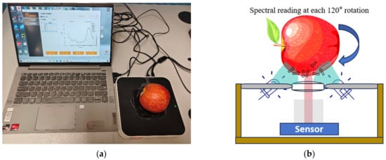
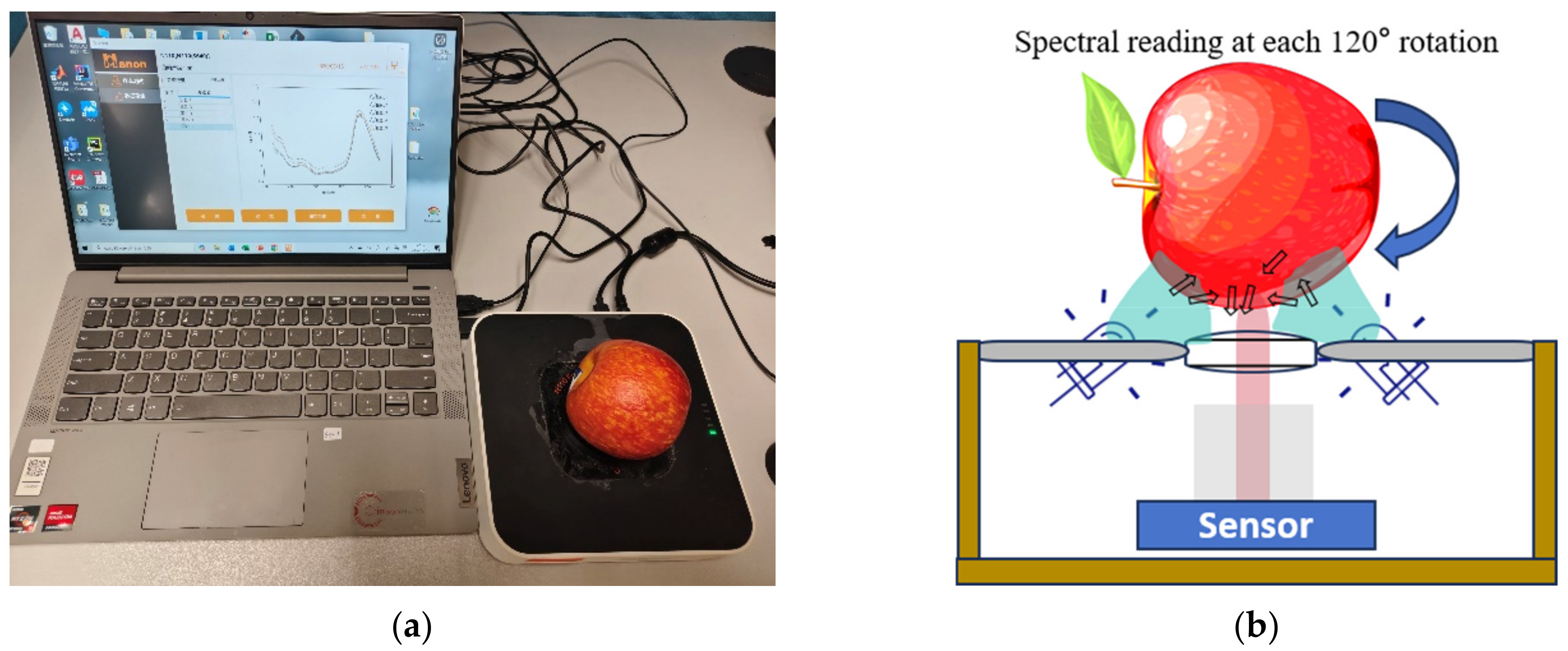
As Figure 1 shown, diffuse interactance spectra were acquired using a portable miniature spectrometer (Model N110, Hanon Instrument Co., Ltd., Jinan, China) equipped with a silicon-based CMOS micro-spectrometer module (Model C11708MA, Hamamatsu Photonics K.K., Hamamatsu, Japan). The instrument covers the 640–1050 nm range with ~1 nm resolution (411 data points per spectrum). Two 2 W tungsten-halogen lamps were positioned symmetrically on either side of the detector probe to provide illumination. Measurement settings were: integration time 0.5 s, 5 co-added scans per acquisition, and initial 5-point smoothing for each spectral reading [26].

For each apple, three replicate spectra were collected at the marked equatorial position by rotating the fruit ~120° (keep the marked region for spectral reading peel coloration and surface curvature) between measurements while gently pressing the probe against the surface to ensure consistent optical contact. The spectrometer was warmed up for 3 min prior to use, and a reference was measured periodically to monitor stability. All measurements were performed in a controlled laboratory environment at 20 ± 2 °C.

2.3. Measurement of Soluble Solids Content (SSC)

Following spectral acquisition, SSC was determined destructively at the marked equatorial position using a handheld digital refractometer (PAL-1, Atago Co., Ltd., Tokyo, Japan; range 0–53 °Brix, resolution 0.1 °Brix). A ~20 g wedge of flesh (about 2 cm depth) was excised, manually pressed with a garlic press to extract juice, which was put onto three refractometers’ prism. The mean of the two closest readings (usually difference ≤ 0.3 °Brix) was used as the reference value. The prism was rinsed with distilled water and dried between measurements. Instrument calibration with distilled water was repeated if discrepancies exceeded 0.2 °Brix.

2.4. Data Analysis

2.4.1. Similarity Assessment of Replicate Spectra

Spectral similarity among the three replicate measurements per apple was quantified using cosine similarity and Mahalanobis distance. Cosine similarity between spectral vectors x_i and x_j is defined as Equation (1):

$$S_{ij}={\displaystyle \frac{{\mathrm{x}}_i\cdot {\mathrm{x}}_j}{‖x_i‖·‖x_j‖}}={\displaystyle \frac{{\displaystyle {\sum }_{k=1}^p}{x}_{ik}{·x}_{jk}}{\sqrt{{\displaystyle {\sum }_{k=1}^p}{x}_{ik}^2} ·\sqrt{{\displaystyle {\sum }_{k=1}^p}{x}_{jk}^2}}}$$

(1)

where p denotes the number of wavelength variables. The Mahalanobis distance between a spectrum x and the mean spectrum $\overline{x}$ of the replicates is computed as Equation (2):

$$D_M=\sqrt{{\left(\mathbf{x}−\overline{\mathbf{x}}\right)}^T{·\mathbf{S}}^{-1}·\left(\mathbf{x}−\overline{\mathbf{x}}\right)}$$

(2)

where S represents the covariance matrix of the replicate sampling spectra. These metrics assess both spectral shape and multivariate dispersion.

2.4.2. Spectral Pretreatments

Spectral pretreatment is essential to improve the signal-to-noise ratio and mitigate physical effects such as scattering, baseline drift, and pathlength variations. Six pretreatments were evaluated: standard normal variate (SNV), multiplicative scatter correction (MSC), first derivative (Savitzky–Golay, 2nd-order polynomial, 5-point window), detrending (2nd-order polynomial subtraction), min–max normalization, and mean centering [27]. A piecewise Savitzky–Golay smoothing (5-point window for 640–950 nm; 9-point for 950–1050 nm) was applied first to address wavelength-dependent noise from the Si-CMOS detector. The optimal pretreatment was selected based on PLS cross-validation performance for both averaged and replicate-spectra datasets.

2.4.3. Multivariate Calibration

Partial least squares (PLS) regression was used as the primary calibration method due to its effectiveness with high-dimensional, collinear spectral data [28]. PLS simultaneously decomposes the spectral matrix and the response vector while maximizing the covariance between latent variables (LVs) and the target analyte. PLS models were optimized using 6-fold cross-validation on the calibration set, with the optimal number of latent variables determined by minimizing the root mean square error of cross-validation (RMSECV). Under k-fold cross-validation, all three replicate spectra of a given apple were always assigned to the same fold, so that no apple ever contributed spectra to both the training and the validation partition within any fold.

2.4.4. Variable Selection

To enhance the predictive performance of the calibration models, two variable selection strategies were compared: uninformative variable elimination (UVE) [29,30] for discrete wavelengths and backward interval PLS (BiPLS) for contiguous spectral intervals [28].

UVE was employed to eliminate discrete wavelengths whose stability fell below that of random Gaussian noise, thereby retaining only those variables capable of adequately reflecting the target attribute [29]. By augmenting the original spectral matrix with artificial noise variables and computing the stability of each regression coefficient, wavelengths exhibiting inferior stability relative to the noise threshold were discarded. This procedure yields a subset of discrete wavelengths that carry genuine chemical information pertinent to SSC prediction.

In the BiPLS method, the full spectrum was divided into n equidistant sub-intervals. PLS models were built sequentially, and the sub-interval whose removal yielded the lowest root mean square error of cross-validation (RMSECV) was eliminated at each iteration [28]. This backward elimination process was repeated until the optimal combination of sub-intervals, yielding the minimum RMSECV, was attained. BiPLS thus identifies contiguous spectral regions that collectively contribute most to the prediction of SSC, while suppressing noisy or redundant intervals [31].

2.4.5. Evaluation Metric

Model performance was evaluated at both the cross-validation and prediction stages using the correlation coefficient (R), root mean square error (RMSE), and mean absolute error (MAE). RMSE measures the average magnitude of prediction errors, and MAE represents the average absolute deviation between predicted and reference values. A well-calibrated model is expected to exhibit high R approaching unity and low RMSE and MAE values, with cross-validation performance moderately superior to or comparable with the prediction set performance to indicate acceptable generalization.

In addition, the residual predictive deviation (RPD) was computed for the prediction set as RPD = SD/RMSEP, where SD is the standard deviation of the reference SSC values of the prediction set (SD = 1.1277 °Brix for the 66 averaged-spectra reference values; SD = 1.1220 °Brix for the 198 replicate-spectra reference values, the three replicates of each apple sharing the same reference value). RPD normalizes the prediction error by the natural spread of the reference values and is widely used to compare models across datasets. Following common interpretation guidelines, RPD < 1.4 indicates poor predictive ability, 1.4 ≤ RPD ≤ 2.0 indicates fair performance suitable for rough screening, and RPD > 2.0 indicates good performance suitable for quantitative screening purposes.

To evaluate the model’s reliability when applied to multiple replicate sampling spectra from individual samples, the concepts of trueness (systematic error) and precision (random error) were adopted. Trueness was quantified by the relative absolute bias (RAB), calculated as the absolute difference between the mean predicted value across replicate spectra and the corresponding reference SSC value, divided by the reference value and expressed as a percentage. A lower RAB indicates higher trueness. Precision was expressed as the relative standard deviation (RSD) of the replicate predictions, computed as the standard deviation of the predicted SSC values across replicate spectra divided by their mean and expressed as a percentage. A lower RSD signifies higher precision. An ideal model should simultaneously achieve low RAB and low RSD, thereby ensuring high overall accuracy for repeated on-site measurements.

$$RAB={\displaystyle \frac{\sqrt{{{\sum }_{k=1}^n(y-\widehat{y_k})}^2}}{\mathrm{n}·\mathrm{y}}}\times 100\%$$

(3)

$$RSD={\displaystyle \frac{\sqrt{{{\sum }_{k=1}^n(\widehat{y_m}-\widehat{y_k})}^2}}{\mathrm{n}·\widehat{y_m}}}\times 100\%, \widehat{y_m}={\displaystyle \frac{1}{n}}·{\sum }_{k=1}^n\widehat{y_k}$$

(4)

where y is the actual measured value; n is the number of repeated spectral acquisition; $\widehat{y_k}$ is the k-th predicted value by the developed regression model.

2.4.6. Software

Data pretreating chemometric modeling and statistical analyses were performed using MATLAB R2025b (MathWorks, Inc., Natick, MA, USA). The PLS regression, UVE, and BiPLS algorithms were implemented using the ChemoToolbox and iToolbox packages [28,32]. Other scripts were developed for spectral similarity computation, cross-validation partitioning, and metric evaluation.

3. Results and Discussions

3.1. Profiles of Spectra

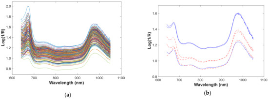
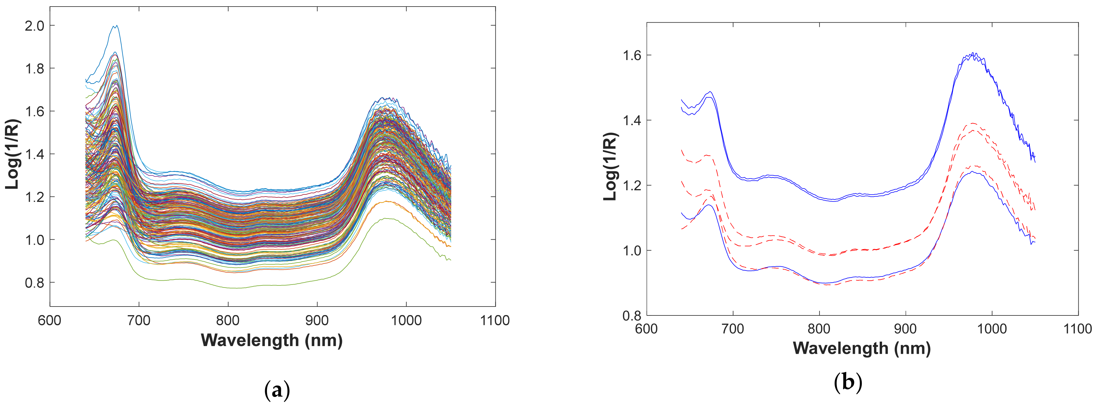
The raw interactance spectra of the Ambrosia apple samples, acquired in the 640–1050 nm range and expressed in log(1/R) units, exhibit a characteristic double-peak profile (Figure 2a). Across the entire spectral range, pronounced inter-sample variability in baseline offset is evident. This variation is primarily attributable to physical differences among specimens, including fruit size, peel coloration, and the resulting optical pathlength and scattering heterogeneity under the interactance geometry.

In the visible-to-NIR transition region (640–750 nm), the spectra display a sharp absorption peak centered at approximately 685 nm. This band corresponds to the red-edge absorption of chlorophyll a located in the apple peel and outer pericarp tissues [13]. The intensity of this 685 nm peak is strongly modulated by peel color: green-skinned apples exhibit higher absorbance values owing to greater chlorophyll concentration, whereas red-skinned specimens show comparatively attenuated peak intensities due to the competitive absorption and masking effects of anthocyanins and carotenoids in the 640–700 nm range [5,13,33]. Consequently, this region encodes not only pigment-related maturity information but also introduces color-dependent spectral variance that must be accounted for during chemometric modeling [8,14].

The most intense absorption band across the entire short-wave NIR window appears at approximately 980 nm and is unequivocally assigned to the second overtone of the O–H stretching vibration of water. Apples typically contain 80–90% moisture, and the strong polar interaction of water molecules with the surrounding cellular matrix produces a broad, asymmetric absorption envelope centered near 980 nm. This band is the dominant spectral signature in the 900–1050 nm interval and is highly sensitive to the total water content, the degree of water binding within cellular compartments, and solute-induced shifts arising from dissolved sugars and organic acids. Because the O–H second overtone partially overlaps with weak C–H combination bands from carbohydrates in the 960–990 nm region, the fine structure around 980 nm also carries indirect information on soluble solids content (SSC). The elevated absorbance values observed in this region, combined with the convergence of spectral curves from different samples, underscore the predominance of water as the primary chromophore in fresh apple tissue.

3.2. Spectral Variability Among Replicate Readings

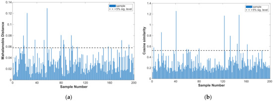
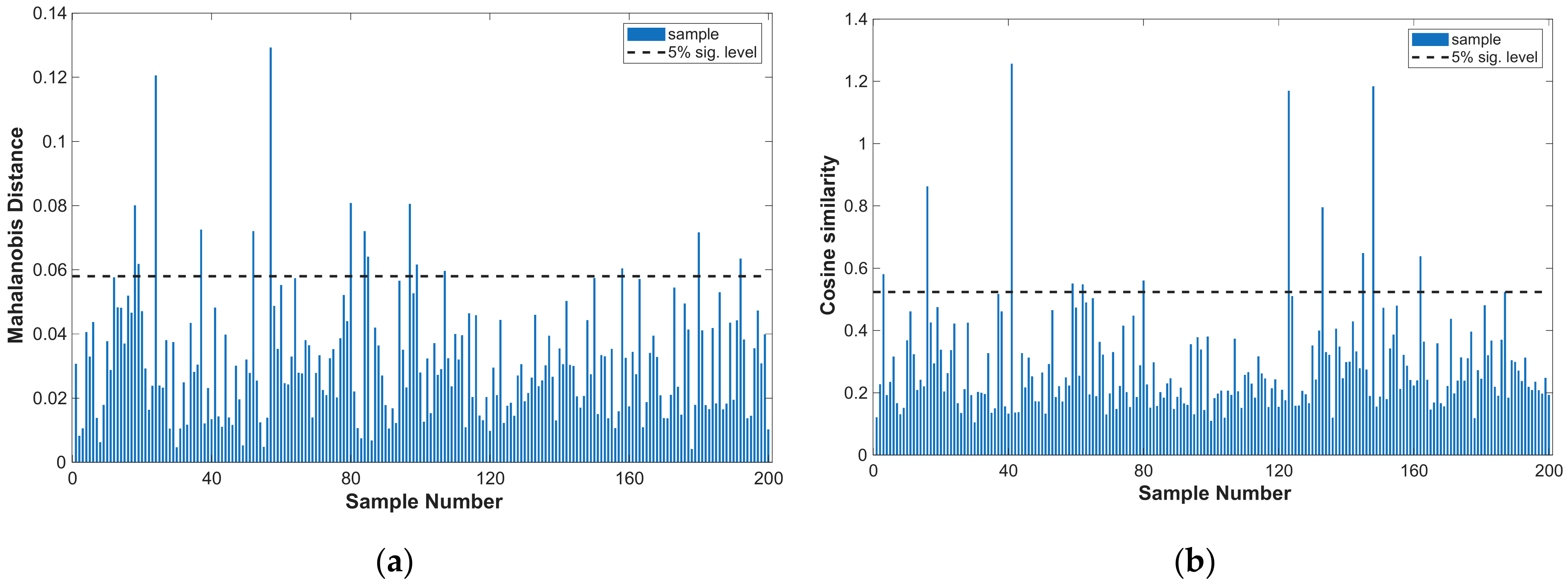
The variability among repeated spectral acquisitions was quantified for each sample using cosine similarity and Mahalanobis distance, and as illustrated in Figure 3, the spectral similarity among replicate measurements varied considerably across the sample cohort, indicating that the degree of spectral reproducibility was sample-dependent rather than uniform. Statistical testing revealed that more than ten samples exhibited statistically significant discrepancies among their replicate spectra, underscoring the prevalence of non-negligible measurement-to-measurement variability under the portable interactance configuration. Notably, the sets of outlier samples identified by the two metrics, cosine similarity and Mahalanobis distance, were not identical, suggesting that these indices capture complementary aspects of spectral dissimilarity: cosine similarity is primarily sensitive to differences in spectral shape and trend, whereas Mahalanobis distance additionally accounts for the covariance structure and multivariate scatter of the spectral data. The non-overlapping outlier sets therefore imply that a single metric alone is insufficient to fully characterize the multidimensional nature of spectral variability.

Figure 2b presents the replicate spectral curves for two representative samples, providing a visual illustration of the observed variability. The discrepancies among repeated measurements manifest in two principal forms: (i) baseline offset and amplitude differences, reflected in the vertical displacement of absorbance values across the entire wavelength range, which primarily arise from inconsistent fruit-to-probe contact pressure, fruit weight-induced detector distance variation, and asymmetric dual-lamp illumination; and (ii) spectral shape and trend divergence, evident in localized differences in peak depth, shoulder definition, and the relative intensity ratios between the 685 nm and 980 nm absorption regions. The coexistence of these amplitude- and shape-based discrepancies indicates that the spectral variability is not merely a simple additive or multiplicative scaling effect, but rather a complex perturbation encompassing both baseline shifts and wavelength-dependent structural distortions.

Such spectral inconsistencies are anticipated to exert deleterious effects on the subsequent chemometric modeling in three respects. First, the trueness (MAE) of the calibration model may be compromised because the training set contains spectral signatures that do not consistently map to the same reference SSC value, thereby blurring the underlying spectral–analyte relationship. Second, the stability of the model, particularly its robustness to minor perturbations in the input space, will be degraded, as the model must accommodate a broader and more heterogeneous spectral distribution for nominally identical samples. Third, and most critically for practical deployment, the precision (repeatability) of predictions for future unknown samples will be diminished, because the model’s output will fluctuate across replicate measurements of the same specimen due to the input spectral variability. Consequently, a user performing repeated on-site measurements of a single apple may obtain discordant SSC predictions, undermining the reliability and trustworthiness of the portable screening system.

In light of these considerations, it explored whether appropriate spectral pretreatments and alternative modeling strategies, specifically, the use of averaged versus multiply sampled spectral data, can mitigate the adverse impact of replicate spectral variability on predictive trueness and precision.

The complete dataset comprising 200 Ambrosia apple samples was randomly partitioned into a calibration set and a prediction set at a ratio of 2:1, yielding 134 samples for model training and 66 samples for external validation. To preserve the integrity of the replicate measurement structure and prevent data leakage, all three replicate spectra acquired from each individual apple were assigned to the same subset; consequently, the 600 spectra (200 samples × 3 replicates) were grouped into 134 calibration samples (402 spectra) and 66 prediction samples (198 spectra) rather than being distributed independently. This block-level partitioning ensures that spectral variability among replicate measurements of the same fruit is consistently represented within either the calibration or the validation phase, thereby enabling an unbiased assessment of the model’s predictive performance when confronted with multiple readings from previously unseen specimens. For each replicate spectrum, the corresponding reference SSC value was identical to that of the parent sample, meaning that the three replicate spectra per apple shared the same target response during model training and evaluation.

3.3. Optimization of Spectral Pretreatments

The raw spectra exhibited a relatively smooth contour below approximately 950 nm, whereas pronounced high-frequency noise fluctuations became evident in the 950–1050 nm region (Figure 2a). This wavelength-dependent degradation in spectral quality is attributable to the inherently lower signal-to-noise ratio (SNR) of silicon-based detectors at the longer-wavelength edge of the short-wave near-infrared (SW-NIR) window, where the quantum efficiency of the Si-CMOS sensor declines markedly.

To address this issue without compromising spectral fidelity, a piecewise Savitzky–Golay smoothing strategy was adopted. A 5-point second-order polynomial window was applied to the 640–950 nm region, where the raw data already exhibited adequate smoothness. A wider 9-point window was employed for the 950–1050 nm region to more effectively suppress the elevated noise. The use of an excessively narrow smoothing window across the entire spectrum proved insufficient for noise suppression in the high-noise tail region, whereas a uniformly large window risked obliterating local spectral features, particularly the subtle shoulders and inflection points that encode chemical information, in the lower-noise region. It has been explicitly verified that this sequence does not distort chemically informative bands. Empirically, comparing the “None” (instrument output only) and “Smooth” rows of

Table 1. Comparisons of different pretreatments on the average and replicate spectra.

Pretreatment	Calibration Set 1 (Average Spectra)				Calibration Set 2 (Replicate Spectra)
	LV	RMSECV	MAE	Rcv	LV	RMSECV	MAE	Rcv
None	12	0.749	0.620	0.854	14	0.689	0.541	0.878
Smooth	15	0.651	0.496	0.892	15	0.677	0.529	0.882
SNV	13	0.671	0.527	0.885	14	0.684	0.533	0.880
MSC	13	0.671	0.528	0.885	14	0.680	0.532	0.881
MC	12	0.665	0.498	0.887	15	0.661	0.518	0.888
Scale	13	0.691	0.532	0.877	15	0.692	0.543	0.877
Detrend	12	0.643	0.484	0.895	12	0.675	0.522	0.883
D1st	5	0.944	0.741	0.755	20	0.901	0.718	0.780
D2nd	7	1.154	0.934	0.598	12	1.098	0.868	0.647

, the piecewise smoothing improved the PLS cross-validation performance for both datasets (averaged set: RMSECV 0.749 → 0.651; replicate set: RMSECV 0.689 → 0.677), indicating no detrimental peak distortion. In addition, the window size of smooth is far narrower than the broad absorption bands of interest (FWHM ≈ 50–100 nm for the 980 nm water band), and no visible distortion of peak or valley bands was observed after smoothing. This adaptive, segment-specific smoothing protocol was applied as the first preprocessing step.

Following piecewise Savitzky–Golay smoothing, six additional pretreatments were systematically evaluated on the averaged spectra to identify the optimal transformation for PLS regression, and the impact of each pretreatment on the PLS calibration performance is summarized in Table 1. The cross-validation performance of PLS models improved appreciably for both the averaged-spectrum and the multiply sampled-spectrum calibration sets. This confirms that the wavelength-adaptive noise suppression preserved chemically informative variance while reducing irrelevant high-frequency perturbations. Notably, first-derivative processing amplified the residual noise, particularly in the 950–1050 nm region, and consequently degraded the model performance relative to the smoothed baseline. This outcome is consistent with the well-documented noise-amplification risk of derivative operations on low-SNR data.

Among the remaining pretreatments, SNV, MSC, and scaling (z-score and min–max normalization) yielded moderate but inconsistent improvements. Their performance varied across the averaged-spectrum and replicate-spectrum calibration sets, suggesting that these scatter correction and normalization methods, while effective for baseline offset compensation, did not fully account for the complex, sample-dependent spectral trends introduced by the interactance geometry and fruit-to-fruit physical heterogeneity. Multiplicative scatter correction (MSC), in particular, exhibited unstable behavior across calibration sets, likely because the single-reference spectrum assumption underlying MSC was violated by the substantial diversity in fruit size, shape, and peel coloration within the cohort.

By contrast, detrending, which fits and subtracts a second-order polynomial from each spectrum to eliminate wavelength-dependent baseline trends, emerged as the most robust and universally effective pretreatment. By explicitly modeling and eliminating the broad, systematic trends attributable to scattering and pathlength variations, detrending effectively decoupled the chemical absorption signals from the physical baseline offsets and spectral shape discrepancies that were particularly prevalent among the replicate measurements. This pretreatment yielded the lowest RMSECV and the highest correlation coefficients for both the averaged-spectrum calibration set and the multiply sampled spectrum calibration set, outperforming SNV, MSC, scaling, and derivative processing in all evaluated configurations. The superiority of detrending is consistent with findings in similar interactance-mode fruit spectra applications, where non-linear baseline trends, rather than simple multiplicative scatter, constitute the dominant physical perturbation. Consequently, detrending was adopted as the definitive pretreatment for all subsequent spectral analyses and model development in this study.

3.4. Results of UVE Variable Selection

UVE was applied to the detrended averaged-spectra and replicate-sampled spectra calibration sets, with the replicate spectra from the prediction set serving as the external validation set in both cases. Four hundred random Gaussian noise variables were appended to the spectral matrix. Wavelengths whose regression coefficient stability fell below the maximum stability of the noise variables were iteratively eliminated. Because the stochastic nature of the appended noise introduces variability into the stability rankings, the UVE procedure was repeated 10 independent runs for each calibration set to ensure reproducibility and mitigate spurious outcomes.

The outcomes of the 10 UVE iterations are summarized in

Table 2. Performance of 10 consecutive UVE runs on averaged spectra.

Run-th	Sel_var.	Calibration Set 1 (134 Spectra)			Prediction Set (198 Spectra)
		RMSECV	MAE	Rcv	RMSEP	MAE	Rp	RPD
1	127	0.554	0.428	0.923	0.828	0.663	0.672	1.354
2	75	0.627	0.475	0.900	0.977	0.770	0.487	1.148
3	71	0.694	0.548	0.876	1.074	0.842	0.281	1.045
4	56	0.681	0.526	0.881	1.057	0.837	0.328	1.061
5	68	0.639	0.511	0.896	0.966	0.775	0.506	1.162
6	66	0.650	0.501	0.892	0.928	0.727	0.559	1.209
7	74	0.642	0.520	0.895	0.758	0.616	0.736	1.481
8	86	0.575	0.451	0.917	0.922	0.728	0.567	1.217
9	123	0.549	0.422	0.925	0.917	0.725	0.573	1.223
10	91	0.543	0.419	0.926	0.848	0.676	0.652	1.323
Avg.	83.7	0.616	0.480	0.903	0.928	0.736	0.536	1.210

and

Table 3. Performance of 10 consecutive UVE runs on replicate sampling spectra.

Run-th	Sel_var.	Calibration Set 1 (402 Spectra)			Prediction Set (198 Spectra)
		RMSECV	MAE	Rcv	RMSEP	MAE	Rp	RPD
1	34	0.702	0.570	0.873	0.711	0.566	0.772	1.578
2	39	0.869	0.681	0.797	0.867	0.695	0.632	1.294
3	55	0.644	0.511	0.894	0.764	0.598	0.731	1.469
4	49	0.865	0.684	0.799	0.882	0.689	0.616	1.273
5	39	0.646	0.523	0.894	0.746	0.593	0.745	1.504
6	35	0.803	0.638	0.830	0.894	0.712	0.601	1.255
7	39	0.901	0.704	0.780	0.838	0.658	0.663	1.339
8	34	0.689	0.544	0.878	0.746	0.602	0.745	1.504
9	25	0.918	0.730	0.770	0.881	0.688	0.617	1.274
10	18	0.894	0.710	0.784	0.871	0.684	0.628	1.289
Avg.	36.7	0.793	0.630	0.830	0.820	0.649	0.675	1.368

. The number of retained wavelengths varied substantially across runs, ranging from a minimum of 18 to a maximum of 127 variables. This reflects the sensitivity of the stability threshold to the specific realization of the appended noise. Notably, the averaged-spectra calibration set consistently yielded a considerably larger pool of selected variables, with a mean of 83.7 wavelengths retained across the 10 runs. In contrast, the replicate-spectrum calibration set produced a markedly more parsimonious subset, averaging only 36.7 wavelengths. This divergence indicates that the expanded training corpus, encompassing the full measurement-to-measurement variability of genuine replicate acquisitions, provided the UVE algorithm with greater statistical power to discriminate chemically informative signals from noise, thereby converging on a tighter and more robust set of predictive variables. Conversely, the averaged-spectrum dataset, having compressed the intra-sample variance into a single representative spectrum per fruit, presented a more limited variance structure, prompting the UVE algorithm to retain a broader and potentially more redundant set of wavelengths.

Because UVE appends randomly generated Gaussian noise variables, each run yields a different variable subset; nevertheless, across repeated runs the selections consistently converge on specific spectral regions, as we reported previously in a 100-run UVE selection-frequency analysis of apricot NIR spectra [34]. Likewise, BiPLS retains different combinations and numbers of intervals depending on the interval partition, since each partition changes the block structure over which the backward elimination operates.

In the cross-validation phase, the UVE-PLS model built on averaged spectra achieved a lower RMSECV of 0.616, compared with 0.793 for the replicate-spectra model. This apparent superiority during internal validation is attributable to the reduced spectral variance and higher signal-to-noise ratio of the averaged data, which facilitate tighter model fitting to the calibration set. However, this performance advantage did not translate to the independent prediction phase. When both models were challenged with the replicate-spectra prediction set, the averaged-spectra model exhibited a marked deterioration, with the RMSEP increasing to 0.928, whereas the replicate-spectra model achieved a substantially lower RMSEP of 0.820, representing an improvement of approximately 11.6%. Furthermore, the replicate-spectra model attained this enhanced prediction accuracy while utilizing less than half the number of input variables (36.7 vs. 83.7 on average). This underscores the efficiency and discriminative power of the sparser variable set derived from the more diverse training data.

It should be noted that the RPD is a ratio metric jointly determined by the prediction error and the standard deviation of the reference values. Because the present samples were commercial fruits of a single cultivar with a naturally narrow SSC spread (SD ≈ 1.12 °Brix in the prediction set), the attainable RPD is compressed even at a low absolute prediction error (RMSEP = 0.677 °Brix). Moreover, the contribution of this study lies in the relative improvement achieved by the multiply sampled replicate calibration strategy under strictly identical experimental conditions, rather than in an absolute performance benchmark. The attained RPD of 1.656 corresponds to screening-grade performance according to the conventional interpretation scheme, which is consistent with the intended on-site screening application of a low-cost portable short-wave NIR instrument.

3.5. Results of BiPLS Variable Selection

BiPLS was applied to the full detrended spectrum to identify optimal contiguous spectral intervals for SSC prediction. The spectrum was divided into successively finer interval configurations ranging from 10 to 20 equidistant sub-intervals. For each configuration, PLS models were built sequentially, and the sub-interval whose removal yielded the lowest root mean square error of cross-validation (RMSECV) was eliminated at each iteration. This backward elimination process was repeated until the optimal combination of sub-intervals, yielding the minimum RMSECV, was attained. The outcomes for the averaged-spectrum and replicate-spectrum calibration sets are summarized in

Table 4. Performance of BiPLS method with runs on averaged spectra.

Intv.	Sel_Intv.	Calibration Set 1 (134 Spectra)			Prediction Set (198 Spectra)
		RMSECV	MAE	Rcv	RMSEP	MAE	Rp	RPD
10	[3;10;5;7;6;8;2]	0.578	0.445	0.916	0.902	0.721	0.592	1.243
11	[6;11;5;3;8;7;9;2]	0.576	0.449	0.917	0.892	0.719	0.604	1.257
12	[8;12;10;6;3;7;9;2]	0.595	0.479	0.911	0.893	0.722	0.603	1.257
13	[7;6;13;9;3;10;8;2]	0.567	0.436	0.919	0.899	0.732	0.595	1.248
14	[3;2;9;14;6;10;4;11]	0.570	0.449	0.918	0.972	0.782	0.496	1.155
15	[6;11;9;4;13;12;10]	0.586	0.439	0.914	0.875	0.690	0.624	1.283
16	[7;5;12;13;3;14;6;11]	0.581	0.447	0.915	0.834	0.675	0.667	1.345
17	12 × 1	0.585	0.461	0.914	0.905	0.726	0.589	1.240
18	12 × 1	0.570	0.437	0.918	0.873	0.696	0.626	1.285
19	13 × 1	0.577	0.448	0.916	0.875	0.703	0.624	1.283
20	12 × 1	0.558	0.450	0.922	0.964	0.777	0.508	1.164
Avg.	0.6277 × 411 = 258	0.577	0.449	0.916	0.899	0.722	0.593	1.249

and

Table 5. Performance of BiPLS runs on replicate sampling spectra.

Intv.	Sel_Intv.	Calibration Set 2 (402 Spectra)			Prediction Set (198 Spectra)
		RMSECV	MAE	Rcv	RMSEP	MAE	Rp	RPD
10	[3;5;7;1;8;6;2]	0.649	0.510	0.893	0.674	0.552	0.798	1.665
11	[2;6;8;3;7;9;1]	0.651	0.511	0.892	0.668	0.547	0.802	1.679
12	[4;11;5;8;3;10;7;9;2]	0.659	0.514	0.889	0.691	0.567	0.787	1.624
13	[4;6;7;9;3;10;8;2]	0.644	0.502	0.895	0.686	0.564	0.790	1.636
14	[14;13;4;9;6;10;8;11;3;2]	0.645	0.507	0.894	0.675	0.556	0.798	1.663
15	[15;14;6;11;4;10;9;12;3;2]	0.653	0.509	0.891	0.685	0.564	0.791	1.638
16	11 × 1	0.652	0.508	0.892	0.682	0.559	0.793	1.644
17	12 × 1	0.634	0.494	0.898	0.667	0.551	0.803	1.683
18	[12;8;3;10;5;13;11;4;14;1]	0.642	0.506	0.895	0.672	0.556	0.800	1.671
19	11 × 1	0.636	0.496	0.897	0.656	0.542	0.810	1.710
20	[12;18;16;5;8;3;17;14;6]	0.641	0.503	0.895	0.696	0.571	0.783	1.611
Avg.	0.6419 × 411 = 264	0.646	0.505	0.894	0.677	0.557	0.796	1.656

, respectively.

To facilitate chemical interpretation, the interval indices in Table 4 and Table 5 can be mapped onto the wavelength axis: the 411 spectral points span 640–1050 nm at ≈1 nm per point, so a division into n equidistant intervals corresponds to ≈410/n nm per interval (e.g., n = 19 → ≈21.6 nm per interval). Mapping the retained intervals onto this axis shows that, for both calibration sets, the selections consistently cover the 680–760 nm region (chlorophyll red-edge/anthocyanin absorption) and the 900–1000 nm region (O–H second overtone of water and overlapping C–H combination bands of carbohydrates), corroborating the band assignments discussed in Section 3.1.

For both calibration sets, the BiPLS procedure retained a substantial majority of the original spectral range, with the selected intervals collectively exceeding half of the total wavelength coverage. Specifically, the mean retained proportions were 62.8% for the averaged-spectrum dataset and 64.2% for the replicate-spectrum dataset. This indicates that the two modeling approaches required comparably broad spectral information when operating at the interval-selection level. Unlike the UVE analysis, where the replicate-spectrum dataset yielded a dramatically sparser variable set, the BiPLS interval-based strategy retained broadly similar spectral proportions for both datasets. This convergence suggests that the evaluation of contiguous spectral blocks, rather than individual wavelengths, necessitates preservation of extended spectral regions to maintain the integrity of chemically informative band shapes and baseline trends.

In the cross-validation phase, the BiPLS-PLS model optimized on averaged spectra achieved a lower RMSECV of 0.577, outperforming the replicate-spectrum model (RMSECV 0.646). In the independent prediction phase, however, the performance ranking reversed markedly: the averaged-spectrum model yielded an RMSEP of 0.899, whereas the replicate-spectrum model achieved a substantially reduced RMSEP of 0.677, representing a considerable improvement in predictive accuracy and generalization capability. This reversal mirrors the pattern observed in the UVE analysis and further demonstrates that the replicate-spectrum calibration strategy, despite its higher cross-validation error, produces models that are more robust and reliable when confronted with the spectral variability inherent in individual replicate measurements.

3.6. Comparisons and Discussions

3.6.1. Replicate Spectral Variability and Calibration Strategy

The replicate spectral measurements acquired at each equatorial position exhibited considerable variability, manifesting as both absorbance intensity discrepancies and spectral shape divergence across the 640–1050 nm range (Figure 3). These perturbations arise from a combination of extrinsic and intrinsic factors inherent to the portable interactance configuration: angular asymmetry of the dual halogen lamp illumination, heterogeneity in apple peel coloration (chlorophyll, anthocyanins, and carotenoids), fruit-to-fruit variation in surface curvature and equatorial diameter, inconsistent probe-to-fruit contact pressure during manual positioning, and subtle differences in detector-to-tissue distance modulated by fruit weight. Collectively, these sources generate spectral signatures at nominally identical measurement points that differ in baseline offset, peak depth, and local spectral slope.

In conventional practice, multiple replicate spectra are arithmetically averaged to enhance the signal-to-noise ratio prior to model development. While averaging reduces noise, it also compresses the spectral diversity representative of real-world measurement conditions, reduces the effective training set size, and filters out perturbations that the model will encounter during field deployment. Algorithmic data augmentation techniques (e.g., spectral shifting, scaling, or noise injection) have been used in some studies to expand the training set. However, such synthetic spectra often remain highly similar to the originals and can lead to overfitting. In contrast, acquiring and directly modeling multiple genuine replicate spectra from each specimen is a cost-effective and physically authentic strategy for low-cost portable spectrometers. This approach captures the true operational variability of the instrument–sample interface, including coupled effects of illumination geometry, tissue optics, and positional uncertainty, without the homogeneity limitations of synthetic augmentation. Consequently, calibration on multiply sampled replicate spectra preserves the natural variance structure and provides the modeling algorithm with a more realistic representation of the prediction-domain data.

3.6.2. Spectral Pretreatment Optimization

The raw spectra exhibited wavelength-dependent noise characteristics attributable to the declining quantum efficiency of the Si-based CMOS detector toward the longer-wavelength edge of the SW-NIR window. Below approximately 950 nm, the spectral contours were smooth and structurally well defined, whereas the 950–1050 nm region displayed pronounced high-frequency fluctuations. A piecewise Savitzky–Golay smoothing strategy (5-point window for 640–950 nm and 9-point window for 950–1050 nm) effectively addressed this heteroscedastic noise profile while preserving chemically informative features.

Comparative evaluation of pretreatments (Table 1) showed that first-derivative processing degraded model performance, particularly in the 950–1050 nm region, by amplifying residual noise. Among other transformations, SNV, MSC, and scaling methods provided moderate but inconsistent improvements across calibration sets. These methods were insufficient to fully address the complex, sample-dependent spectral trends introduced by the interactance geometry and physical heterogeneity of the samples. MSC, in particular, showed unstable performance, likely because its single-reference spectrum assumption was violated by the diversity in fruit size, shape, and peel coloration.

Detrending was adopted as the unified pretreatment for both datasets. It achieved the best cross-validation statistics on the averaged-spectrum set (RMSECV 0.643, Rcv 0.895); on the replicate-spectrum set, mean centering was marginally better (RMSECV 0.661, Rcv 0.888 versus 0.675 and 0.883 for detrending), but the relative difference is approximately 2%—within the variability among cross-validation folds and not statistically significant. Because a fair strategy comparison requires a common pretreatment, and because detrending mechanistically removes the broad, wavelength-dependent baseline trends caused by scattering and pathlength variations (the dominant physical perturbation identified in the replicate measurements), detrending was therefore adopted for all subsequent analyses.

3.6.3. Variable Selection and Model Comparison

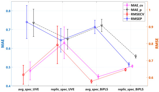
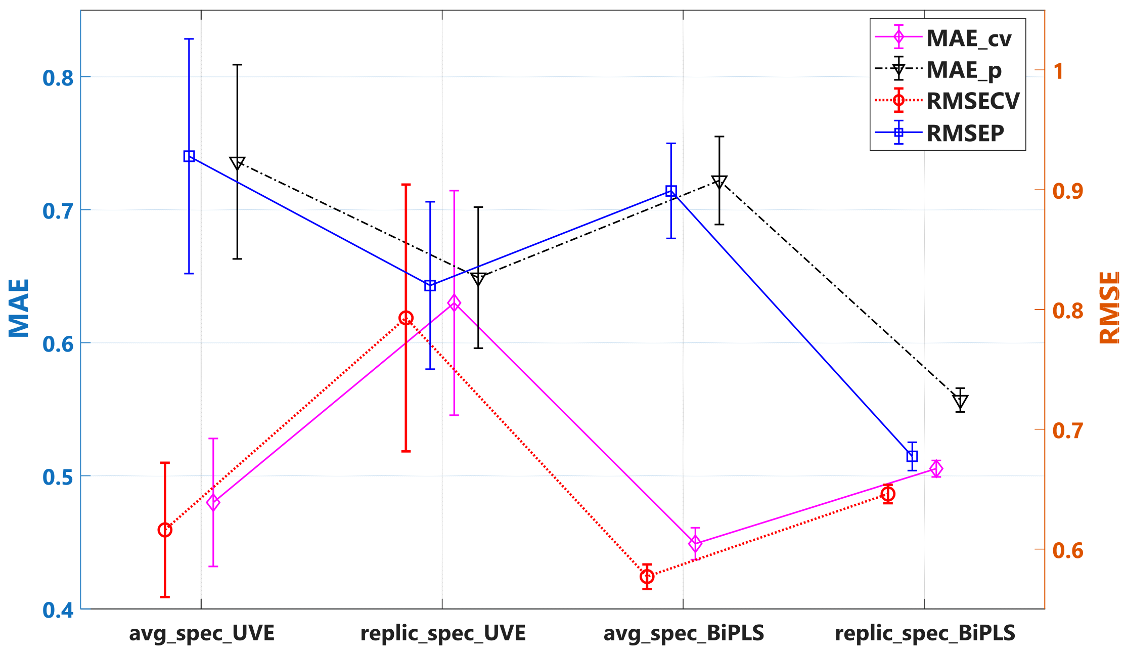
Both UVE and BiPLS variable selection strategies were applied to the detrended averaged-spectrum and replicate-spectrum calibration sets, using the replicate-spectrum prediction set as the common external benchmark. As shown in Figure 4, a consistent pattern emerged across both approaches: models built on averaged spectra achieved lower cross-validation errors (UVE: RMSECV 0.616; BiPLS: RMSECV 0.577) but showed marked degradation in independent prediction (UVE: RMSEP 0.928; BiPLS: RMSEP 0.899). In contrast, models trained on multiply sampled replicate spectra, despite higher RMSECV values (UVE: 0.793; BiPLS: 0.646), generalized substantially better to unseen replicate spectra (UVE: RMSEP 0.820; BiPLS: RMSEP 0.677). This reversal indicates that averaged-spectrum models tend to overfit to the compressed variance structure of averaged data, while replicate-spectrum models learn more generalizable spectral–SSC relationships by incorporating authentic measurement variability during training.

The same ranking is reflected in the RPD values. Using the standard deviations of the prediction-set reference SSC values (SD = 1.1220 °Brix for the 198 replicate-spectra values), the RPD values of the four models are 1.21 (UVE, averaged), 1.249 (BiPLS, averaged), 1.368 (UVE, replicate) and 1.656 (BiPLS, replicate). Both averaged-spectra models fall below the RPD = 1.4 threshold, indicating limited predictive ability for screening purposes. The replicate-spectra models perform markedly better: the UVE model approaches the 1.4 threshold, and the BiPLS model reaches 1.656, within the “fair” band (1.4–2.0) regarded as suitable for rough screening. The 24.7% RMSEP reduction achieved by the replicate-BiPLS model thus translates directly into a proportionally higher RPD, confirming its superior practical utility for on-site screening.

The two selection methods differed in variable retention behavior. UVE produced a dramatically sparser model from the replicate-spectrum dataset (mean 36.7 vs. 83.7 wavelengths), demonstrating that the larger, more diverse training set enabled more confident identification of informative variables. BiPLS, however, retained broadly comparable spectral proportions for both datasets (approximately 63–64% of the spectrum). This difference arises because BiPLS evaluates contiguous spectral blocks, requiring preservation of extended regions to maintain chemically informative band shapes and trends, whereas UVE operates at the individual wavelength level and can prune more aggressively with richer training data.

The BiPLS replicate-spectrum model provided the largest improvement (25.3% RMSEP reduction relative to the averaged model) and consistently outperformed the UVE-PLS model across the prediction set (mean RMSEP 0.677 vs. 0.820). This superiority stems from BiPLS’s ability to capture robust, contiguous spectral features that collectively encode SSC-related chemical information, leading to more stable PLS regression in the presence of replicate variability.

3.6.4. Trueness and Precision of Replicate Predictions

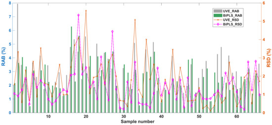
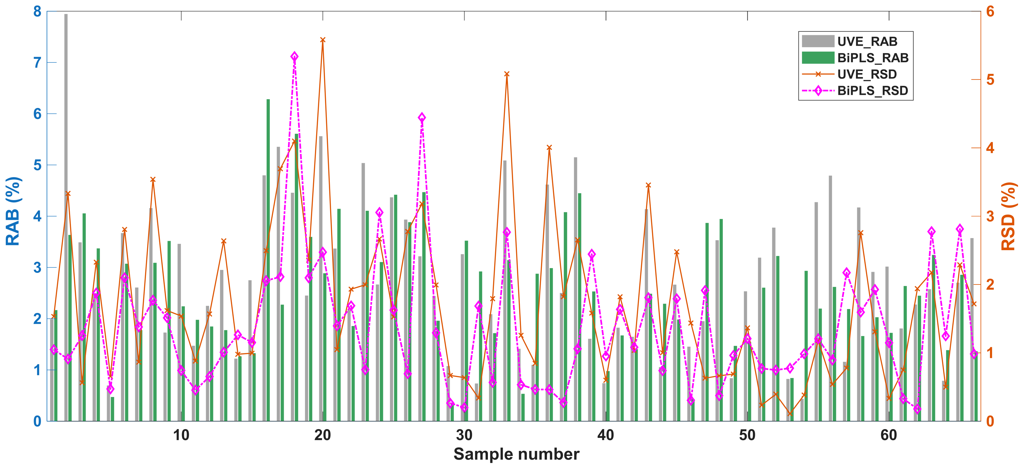
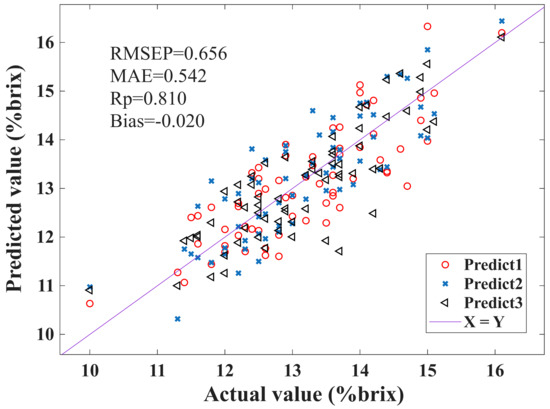
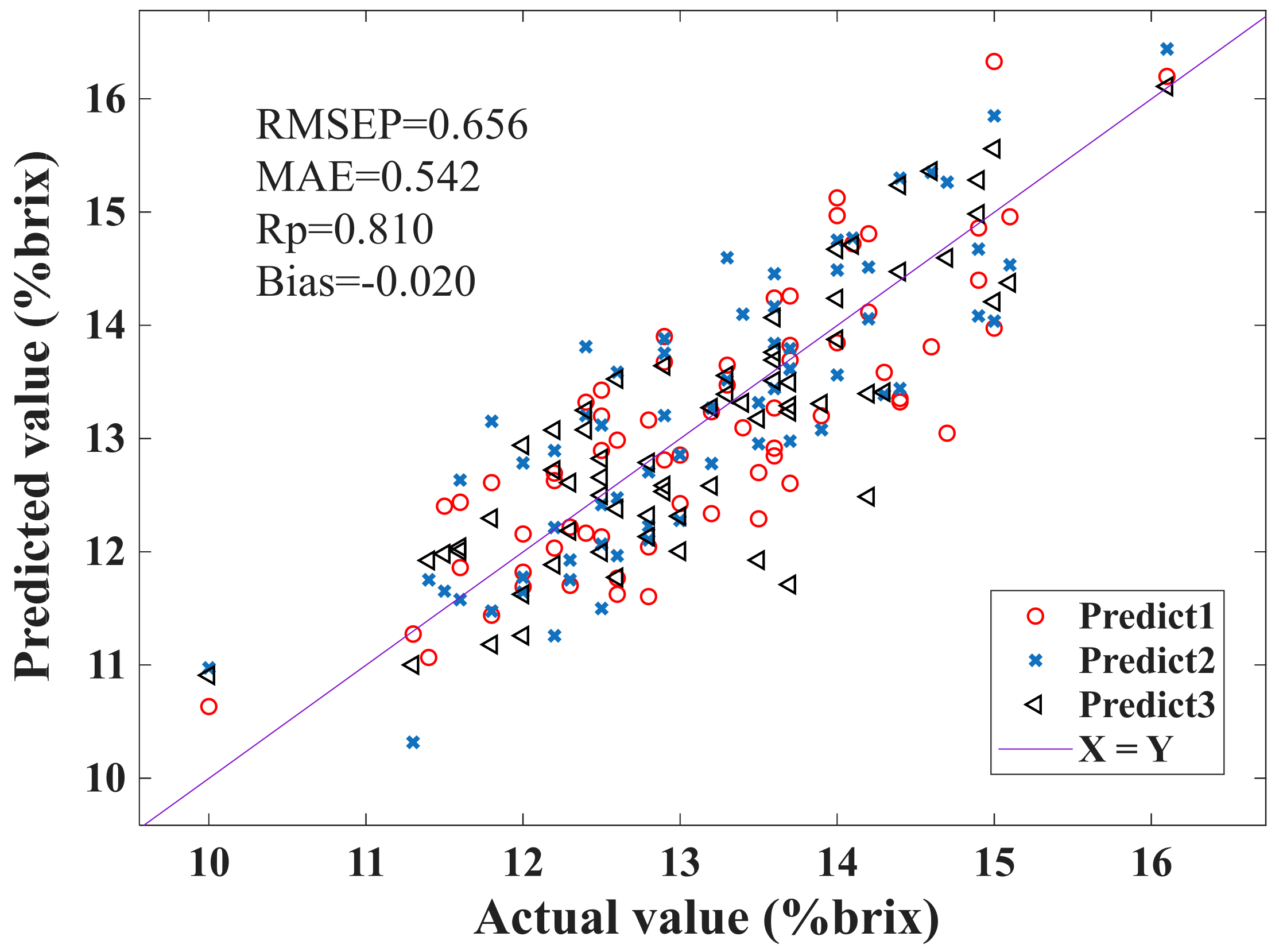
To assess practical reliability for repeated on-site measurements, model performance was evaluated in terms of trueness (systematic bias) and precision (random repeatability). As shown in Figure 5, the BiPLS model developed on replicate spectra exhibited lower relative absolute bias (RAB) and lower relative standard deviation (RSD) across the 66-sample prediction set compared with the UVE-PLS model. These results demonstrate that the BiPLS model delivers predictions closer to the reference SSC values (higher trueness) while producing more consistent outcomes across repeated spectral acquisitions of the same specimen (higher precision). Figure 6 shows the scatter plot of the spectral BiPLS model for predicting apple’s SSC, exhibiting the consistency between three spectral predictions.

The superior trueness and precision of the BiPLS model can be attributed to its interval-based variable retention strategy. By preserving contiguous spectral regions encompassing the full band shapes of O–H and C–H absorption features, BiPLS maintains a more stable regression coefficient structure that is less susceptible to localized noise or minor wavelength shifts. In contrast, the sparse discrete wavelengths selected by UVE are more vulnerable to spectral displacements and intensity fluctuations, resulting in greater prediction variance under operational replicate conditions.

4. Conclusions

This study investigated calibration strategies for predicting soluble solids content (SSC) in Ambrosia apples using a low-cost, portable silicon-based short-wave near-infrared (SW-NIR) spectrometer operating in the 640–1050 nm range under interactance geometry. Replicate spectral acquisitions at the same equatorial position showed substantial variability in both intensity and spectral shape. These discrepancies originated from asymmetric dual-lamp illumination, peel color heterogeneity, and inconsistent probe-to-sample contact.

Conventional averaging of replicate spectra compressed this operational variability, reducing the effective training set size and predisposing models to overfitting. In contrast, directly incorporating multiply sampled replicate spectra preserved the authentic variance structure encountered in real-world measurements, leading to improved generalization performance. Among the pretreatments tested, detrending most effectively removed scattering-induced baseline trends and decoupled chemical absorption signals from physical effects.

Both uninformative variable elimination (UVE) and backward interval partial least squares (BiPLS) variable selection confirmed a consistent pattern: models calibrated on replicate spectra, despite higher cross-validation errors, achieved substantially better prediction accuracy on unseen replicate measurements compared with models built on averaged spectra. The BiPLS model trained on replicate spectra delivered the best overall performance, with a mean RMSEP of 0.677 °Brix (minimum 0.656 °Brix), Rp = 0.796, and RPD = 1.656. It also exhibited superior trueness (lower relative absolute bias, RAB) and precision (lower relative standard deviation, RSD) across the 66-sample prediction set.

Finally, it should be acknowledged that the models developed in this study achieve screening-grade rather than laboratory-grade quantitative performance. The multiply sampled replicate calibration strategy proposed here is orthogonal to the choice of chemometric algorithms: PLS was adopted as a baseline to isolate the strategy effect, and combining the strategy with more effective variable-selection methods (e.g., CARS or genetic algorithms) or non-linear modeling approaches (e.g., support vector regression or ensemble methods) is expected to further improve the predictive performance. This will be investigated in our future work.

References

- Walsh, K.B.; McGlone, V.A.; Han, D.H. The uses of near infra-red spectroscopy in postharvest decision support: A review. Postharvest Biol. Technol. 2020, 163, 111139. [Google Scholar] [CrossRef] [Scilit]
- Gidado, M.J.; Nagoor Gunny, A.A.; Gopinath, S.C.B.; Devi, M.; Ibrahim, A.M. Artificial intelligence and machine learning in postharvest fruit quality assessment: Current challenges, recent advances, and future prospects. J. Stored Prod. Res. 2026, 116, 102959. [Google Scholar] [CrossRef] [Scilit]
- Moura, P.C.; Vassilenko, V. Contemporary ion mobility spectrometry applications and future trends towards environmental, health and food research: A review. Int. J. Mass Spectrom. 2023, 486, 117012. [Google Scholar] [CrossRef] [Scilit]
- Nobari Moghaddam, H.; Tamiji, Z.; Akbari Lakeh, M.; Khoshayand, M.R.; Haji Mahmoodi, M. Multivariate analysis of food fraud: A review of NIR based instruments in tandem with chemometrics. J. Food Compos. Anal. 2022, 107, 104343. [Google Scholar] [CrossRef] [Scilit]
- Beć, K.B.; Grabska, J.; Huck, C.W. In silico NIR spectroscopy—A review. Molecular fingerprint, interpretation of calibration models, understanding of matrix effects and instrumental difference. Spectrochim. Acta Part A Mol. Biomol. Spectrosc. 2022, 279, 121438. [Google Scholar] [CrossRef] [Scilit] [PubMed]
- Vladimir, F.; Levkovich, N.V.; Shuliko, K.I. Diffuse Reflectance Spectrophotometers Based on C12880MA and C11708MA Mini-Spectrometers Hamamatsu. Devices Methods Meas. 2022, 13, 93–104. [Google Scholar] [CrossRef] [Scilit]
- Walsh, K.B.; Blasco, J.; Zude-Sasse, M.; Sun, X. Visible-NIR ‘point’ spectroscopy in postharvest fruit and vegetable assessment: The science behind three decades of commercial use. Postharvest Biol. Technol. 2020, 168, 111246. [Google Scholar] [CrossRef] [Scilit]
- de Oliveira, G.A.; Bureau, S.; Renard, C.M.-G.C.; Pereira-Netto, A.B.; de Castilhos, F. Comparison of NIRS approach for prediction of internal quality traits in three fruit species. Food Chem. 2014, 143, 223–230. [Google Scholar] [CrossRef] [Scilit] [PubMed]
- Nicolai, B.M.; Beullens, K.; Bobelyn, E.; Peirs, A.; Saeys, W.; Theron, K.I.; Lammertyn, J. Nondestructive measurement of fruit and vegetable quality by means of NIR spectroscopy: A review. Postharvest Biol. Technol. 2007, 46, 99–118. [Google Scholar] [CrossRef] [Scilit]
- Wang, X.; Chen, X. Improving fruit variety classification using near-infrared spectroscopy and deep learning techniques. J. Food Compos. Anal. 2025, 140, 107243. [Google Scholar] [CrossRef] [Scilit]
- Mohawesh, R.; Xu, S.; Springer, M.; Jararweh, Y.; Al-Hawawreh, M.; Maqsood, S. An explainable ensemble of multi-view deep learning model for fake review detection. J. King Saud Univ. Comput. Inf. Sci. 2023, 35, 101644. [Google Scholar] [CrossRef] [Scilit]
- Mohammed, A.; Kora, R. A comprehensive review on ensemble deep learning: Opportunities and challenges. J. King Saud Univ. Comput. Inf. Sci. 2023, 35, 757–774. [Google Scholar] [CrossRef] [Scilit]
- Pasquini, C. Near infrared spectroscopy: A mature analytical technique with new perspectives—A review. Anal. Chim. Acta 2018, 1026, 8–36. [Google Scholar] [CrossRef] [Scilit] [PubMed]
- Monnier, G.F. A review of infrared spectroscopy in microarchaeology: Methods, applications, and recent trends. J. Archaeol. Sci. Rep. 2018, 18, 806–823. [Google Scholar] [CrossRef] [Scilit]
- Dong, W.; Wang, X.; Huang, Z.; Ye, C.; Wang, T.; Zhang, H.; Wang, Z.; Li, W. On-Line Monitoring of Guizhi Fuling Capsules and Tablets Dissolution Behavior Using Near-Infrared Spectroscopy Combined with Chemometrics. J. Anal. Test. 2025, 9, 240–249. [Google Scholar] [CrossRef] [Scilit]
- Zhao, Y.; Zhou, L.; Wang, W.; Zhang, X.; Gu, Q.; Zhu, Y.; Chen, R.; Zhang, C. Visible/near-infrared Spectroscopy and Hyperspectral Imaging Facilitate the Rapid Determination of Soluble Solids Content in Fruits. Food Eng. Rev. 2024, 16, 470–496. [Google Scholar] [CrossRef] [Scilit]
- Chen, D.; Hu, B.; Shao, X.G.; Su, Q.D. Removal of major interference sources in aqueous near-infrared spectroscopy techniques. Anal. Bioanal. Chem. 2004, 379, 143–148. [Google Scholar] [CrossRef] [Scilit] [PubMed]
- Schaare, P.N.; Fraser, D.G. Comparison of reflectance, interactance and transmission modes of visible-near infrared spectroscopy for measuring internal properties of kiwifruit (Actinidia chinensis). Postharvest Biol. Technol. 2000, 20, 175–184. [Google Scholar] [CrossRef] [Scilit]
- Grassi, S.; Alamprese, C. Advances in NIR spectroscopy applied to process analytical technology in food industries. Curr. Opin. Food Sci. 2018, 22, 17–21. [Google Scholar] [CrossRef] [Scilit]
- Olumegbon, I.A.; Oloyede, A.; Afara, I.O. Near-infrared (NIR) spectroscopic evaluation of articular cartilage: A review of current and future trends. Appl. Spectrosc. Rev. 2016, 52, 541–559. [Google Scholar] [CrossRef] [Scilit]
- Porep, J.U.; Kammerer, D.R.; Carle, R. On-line application of near infrared (NIR) spectroscopy in food production. Trends Food Sci. Technol. 2015, 46, 211–230. [Google Scholar] [CrossRef] [Scilit]
- Kim, H.J.; Ryu, J.; Kim, G.; Jo, C. Enhancement of non-destructive chicken freshness prediction using Vis/NIR spectroscopy through wavelength selection and data augmentation. LWT 2025, 221, 117602. [Google Scholar] [CrossRef] [Scilit]
- Wang, Y.; Zhao, C.; Tian, H.; Xing, Z.; Yue, X.; Liu, S.; He, Y.; Bai, J.; Hao, L.; Zhu, M.; et al. NIRS-based detection advances in agriculture: Data enhancement, characteristic wavelength selection and modelling techniques. Spectrochim. Acta Part A Mol. Biomol. Spectrosc. 2010, 343, 126611. [Google Scholar]
- Bai, Y.; Xiong, Y.; Huang, J.; Zhou, J.; Zhang, B. Accurate prediction of soluble solid content of apples from multiple geographical regions by combining deep learning with spectral fingerprint features. Postharvest Biol. Technol. 2019, 156, 110943. [Google Scholar] [CrossRef] [Scilit]
- Afonso, A.M.; Antunes, M.D.; Cruz, S.; Cavaco, A.M.; Guerra, R. Non-destructive follow-up of ‘Jintao’ kiwifruit ripening through VIS-NIR spectroscopy—Individual vs. average calibration model’s predictions. Postharvest Biol. Technol. 2022, 188, 111895. [Google Scholar] [CrossRef] [Scilit]
- Yuan, L.-M.; Liu, Y.; Gao, F.; Jiang, Q.; Ji, H.; Chen, X.; Chen, X.; Zhu, F. Prediction of bayberry SSC by ensemble model with random frog successively selected from the residual vis-NIR spectra. Food Control 2025, 178, 111525. [Google Scholar] [CrossRef] [Scilit]
- Chen, X.; Xie, Z.; Tauler, R.; He, Y.; Nie, P.; Peng, Y.; Shu, L.; Ali, S.; Huang, G.; Shi, W.; et al. An automated preprocessing framework for near infrared spectroscopic data. Chemom. Intell. Lab. Syst. 2025, 267, 105542. [Google Scholar] [CrossRef] [Scilit]
- Norgaard, L.; Saudland, A.; Wagner, J.; Nielsen, J.P.; Munck, L.; Engelsen, S.B. Interval partial least-squares regression (iPLS): A comparative chemometric study with an example from near-infrared spectroscopy. Appl. Spectrosc. 2000, 54, 413–419. [Google Scholar] [CrossRef] [Scilit]
- Centner, V.; Massart, D.L.; de Noord, O.E.; de Jong, S.; Vandeginste, B.M.; Sterna, C. Elimination of uninformative variables for multivariate calibration. Anal. Chem. 1996, 68, 3851–3858. [Google Scholar] [CrossRef] [Scilit] [PubMed]
- Centner, V. 3.15—Multivariate Approaches: UVE-PLS. In Comprehensive Chemometrics, 2nd ed.; Brown, S., Tauler, R., Walczak, B., Eds.; Elsevier: Oxford, UK, 2009; pp. 309–316. [Google Scholar]
- Mehmood, T.; Liland, K.H.; Snipen, L.; Sæbø, S. A review of variable selection methods in Partial Least Squares Regression. Chemom. Intell. Lab. Syst. 2012, 118, 62–69. [Google Scholar] [CrossRef] [Scilit]
- de Araújo Gomes, A.; Azcarate, S.M.; Diniz, P.H.G.D.; de Sousa Fernandes, D.D.; Veras, G. Variable selection in the chemometric treatment of food data: A tutorial review. Food Chem. 2022, 370, 131072. [Google Scholar] [CrossRef] [Scilit] [PubMed]
- Zou, X.B.; Zhao, J.W.; Povey, M.J.W.; Holmes, M.; Hanpin, M. Variables selection methods in near-infrared spectroscopy. Anal. Chim. Acta 2010, 667, 14–32. [Google Scholar] [CrossRef] [Scilit] [PubMed]
- Gao, F.; Xing, Y.; Li, J.; Guo, L.; Sun, Y.; Shi, W.; Yuan, L. Prediction of Total Soluble Solids in Apricot Using Adaptive Boosting Ensemble Model Combined with NIR and High-Frequency UVE-Selected Variables. Molecules 2025, 30, 1543. [Google Scholar] [CrossRef] [Scilit] [PubMed]
Disclaimer/Publisher’s Note: The statements, opinions and data contained in all publications are solely those of the individual author(s) and contributor(s) and not of MDPI and/or the editor(s). MDPI and/or the editor(s) disclaim responsibility for any injury to people or property resulting from any ideas, methods, instructions or products referred to in the content. |
© 2026 by the authors. Licensee MDPI, Basel, Switzerland. This article is an open access article distributed under the terms and conditions of the Creative Commons Attribution (CC BY) license.