SDRMixer: A Lightweight Dynamic Response Mixer for Deployable Mixed-Gas Quantification Using Sensor Arrays

Abstract

Low-cost gas sensor arrays are attractive for mixed-gas monitoring, but deployment-oriented modeling remains challenging because mixed-gas responses are nonlinear, cross-sensitive, and strongly dependent on sensor dynamic states. Existing electronic-nose models often rely on handcrafted response descriptors or generic sequential networks, which may either compress transient response information or introduce unnecessary computational cost. This work proposes SDRMixer, a lightweight sensor-specific framework for mixed-gas concentration quantification. SDRMixer uses a parameter-free sparse dynamic response encoding to organize the original sensor response, baseline-referenced excitation, and smoothed response kinetics into a physically meaningful dynamic response field. A compact temporal-feature mixer is then applied over fixed response-stage tokens for simultaneous multi-gas regression. To improve calibration coverage, a response-consistent augmentation strategy is used during model training. The proposed framework is evaluated on a previously reported mixed-gas sensor array dataset containing NO₂, NH₃, CH₄, and CO₂ mixtures. Both augmentation-enriched calibration domain benchmarking and original-measurement-based validation are conducted to assess prediction performance, computational efficiency, and stability on measured calibration samples. The results show that SDRMixer provides a good trade-off between accuracy and efficiency compared with generic deep learning architectures and compact gas-sensing baselines. These findings indicate that explicit dynamic response encoding combined with lightweight temporal-feature mixing is an effective modeling strategy for compact mixed-gas quantification within the investigated calibration domain.

1. Introduction

Gas sensor arrays and electronic noses are widely adopted for environmental monitoring, industrial safety, indoor-air assessment, and breath analysis because they combine compact sensing hardware with multivariate pattern recognition. However, their core limitation lies in poor selectivity: metal-oxide semiconductor (MOS) and related chemiresistive gas sensors respond to several analytes, and their signals are further affected by competitive adsorption, temperature and humidity [1,2]. Gas sensor arrays can address this limitation by combining partially selective channels, including cross-sensitive nanowire arrays and material-engineered orthogonal arrays [3,4]. Recent highly integrated and low-power electronic noses further demonstrate the feasibility of compact array hardware [5]. Nevertheless, cross-channel interference, device-to-device variation, and heavy calibration overhead still pose major obstacles to practical field deployment. Beyond environmental and industrial scenarios, mixed-gas analysis is also important in biomedical breath sensing, where human exhaled breath contains complex volatile organic compound mixtures related to physiological and pathological states. A recent review on machine-learning-assisted gas sensor arrays has highlighted their potential for non-invasive medical diagnosis, including respiratory, metabolic, hepatobiliary, gastrointestinal, and nervous-system diseases [6]. These applications further demonstrate that sensor array models must not only identify gas patterns or disease classes, but also preserve concentration-dependent response information when quantitative analysis is required. Therefore, mixed-gas concentration regression is a more demanding task than multi-gas classification, because it requires continuous multi-output estimation from overlapped and cross-sensitive sensor responses.

Accordingly, mixed-gas quantification requires the simultaneous estimation of multiple gas concentrations from heavily overlapped sensor responses. Early research realized quantitative analysis of binary and ternary gas mixtures via thick-film sensor arrays, tapped-delay response characterization, and traditional chemometric regression algorithms [7,8]. Subsequent studies extended array-based sensing techniques to multicomponent gas detection, indoor pollutant monitoring, and chemically complex mixtures such as NO, NO₂, C₃H₈ and NH₃ mixtures [9,10,11]. These studies established that array-level information can support quantitative analysis, but they also showed that the mapping from response to concentration depends strongly on the selected sensors, calibration mixtures, and response descriptors.

A common strategy is to extract steady-state or handcrafted descriptors, such as peak response, response slope, area, response time, and recovery time, and then apply Partial Least Squares Regression, Support Vector Regression, stacking, broad learning, or related chemometric models [10,12,13]. Such approaches feature low computational complexity and perform well with limited calibration datasets. However, when the full adsorption–desorption response trajectory is compressed into fixed handcrafted feature sets, part of the transient kinetic information may be simplified or lost. This drawback becomes particularly prominent in complex mixed-gas environments, where inter-channel signal enhancement, suppression effects, and non-monotonic concentration–response relationships are prevalent. Dynamic sensor responses provide an additional source of chemical information. Previous tapped-delay models showed that temporal histories improve concentration estimation in gas mixtures, while one-dimensional convolutional analysis of sensor fluctuations demonstrated that time series structure can distinguish binary mixtures [8,14]. Neural regression and 1D-Convolutional Neural Network (CNN) methods have also been used for gas concentration analysis and mixture component estimation [15,16]. These studies collectively confirm the value of transient response information for quantitative gas sensing. Recent chemiresistive electronic-nose studies also analyzed dynamic resistance responses and calibration curves with statistical learning methods such as PCA to discriminate single gases and gas mixtures, further supporting the usefulness of transient response information in array-based gas analysis [17]. However, these studies mainly focus on gas or mixture discrimination, whereas simultaneous mixed-gas concentration regression requires continuous multi-output estimation and a more structured representation of concentration-dependent transient responses. Even so, most existing methods either rely on manually engineered temporal features or adopt generic sequence networks to implicitly learn baseline characteristics, response amplitude, and kinetic properties, lacking explicit physical interpretability.

To address such limitations, more expressive neural models have therefore been introduced for gas-array analysis. Neural networks have been used for mixture identification, joint gas recognition and concentration estimation, hybrid 3D-CNN regression, and optimized mixed-gas detection [18,19,20,21]. Temporal-convolutional models can improve concentration prediction under changing conditions, and batch-uniform arrays combined with deep learning have achieved high real-time multi-gas identification accuracy [22,23]. The primary strength of these deep models lies in their capability to model nonlinear cross-channel interaction relationships. However, they suffer from inherent drawbacks: excessive parameter volume, high computational overhead, and heavy reliance on large-scale calibration data. Moreover, superior classification performance cannot be directly transferred to the task of simultaneous multi-gas concentration regression.

Regardless of model architecture, calibration remains a critical bottleneck for practical gas sensor system deployment. Compared with exhaustive grid sampling strategies, random-mixture calibration can more efficiently cover the concentration parameter space [24], and state-of-the-art mixed-gas calibration schemes improve measurement accuracy by constructing information-rich calibration sample sets [25]. Data augmentation, interpolation, and extrapolation have also been explored to construct practical concentration-prediction models [26], while transfer learning can reduce calibration time between MOS sensor systems [27]. Nevertheless, synthetic and transferred calibration data are inherently constrained by the original calibration domain, making model performance vulnerable to sensor drift and unknown interfering gases in long-term field operation [28].

Based on the above analysis, this work identifies and addresses key practical gaps in existing mixed-gas-sensing systems. A deployable multi-gas quantification model is required to preserve physically meaningful transient response information, capture nonlinear cross-channel interactions, deliver stable performance with limited calibrated samples, and maintain a lightweight architecture for resource-constrained edge sensing devices. Traditional compact chemometric models may not fully preserve transient kinetic information when relying on compressed descriptors, while generic deep sequence models often introduce redundant computational and data costs. Different from arbitrary long sequence data, gas sensor responses exhibit structured patterns with distinguishable baseline states, gas-induced excitation variations, and stable response/recovery kinetics, which provides a solid physical foundation for targeted lightweight model design. This work proposes SDRMixer, a lightweight sensor-customized framework for the simultaneous quantification of NO₂, NH₃, CH₄, and CO₂. A parameter-free sparse dynamic response encoding (SDRE) exposes the original response, baseline-referenced change, and smoothed kinetic component before learning. A compact temporal-feature mixer then processes fixed response-stage tokens for multi-gas regression. Response-consistent CalibGrad augmentation is used to improve calibration coverage during training. On the four-gas sensor array dataset reported by our previous work [29], under the augmentation-enriched calibration domain benchmarking setting, SDRMixer achieves a normalized mean absolute error (MAE) of 0.0181 and an R² of 0.9872 with 48.7 k parameters and 1.00 M floating-point operations (FLOPs) per sample. In addition, original-measurement-based validation using only the 110 experimental measurements further evaluates the stability of SDRMixer on real measured calibration samples. Therefore, this work comprehensively evaluated SDRMixer from the perspectives of balancing accuracy and efficiency, as well as actual sample stability, further demonstrating its practical potential for deployment-oriented mixed-gas-sensing systems within the investigated calibration domain.

2. Data and Methods

2.1. Dataset Origin and Response Window

The mixed-gas dataset originates from our previously reported four-sensor array measurements for the quantitative analysis of NO₂, NH₃, CH₄, and CO₂ mixtures [29]. The array consists of four partially selective metal-oxide sensing materials, namely In₂O₃-, Pd-ZnO-, Au-SnO₂-, and Pd-LaFeO₃-based channels. These materials were selected according to their nominal sensitivities to NO₂, NH₃, CH₄, and CO₂, respectively; however, they are not intended to function as fully independent single-gas sensors under mixed-gas exposure. As demonstrated in our previous work [29], under single-gas exposure, the selected sensing materials exhibited good response characteristics toward their corresponding target gases, confirming that the four sensing channels provide meaningful target-related gas response information for the investigated gas system. During gas testing, the sensing channels were operated at their respective working temperatures of 170 °C, 220 °C, 250 °C, and 250 °C under 50% relative humidity. The concentration ranges were 0.1–10 ppm for NO₂, 0.1–50 ppm for NH₃, 50–5000 ppm for CH₄, and 50–10,000 ppm for CO₂. A total of 110 mixed-gas concentration combinations were measured using the customized sensor array testing system. Each sample contains a four-component concentration label and four corresponding transient response curves. Therefore, the input information used in this work is a multi-channel dynamic response window rather than a single steady-state response descriptor. The measured response windows are used as model inputs to simultaneously predict the concentrations of the four gases. Each window covers both the rising response and recovery processes, and after normalization, each input sample is represented as a 4 × 180 response matrix. All data processing, model training, and visualization were conducted using Python 3.10.13 (Python Software Foundation, Wilmington, DE, USA) and PyTorch 2.8.0 (Meta AI, Menlo Park, CA, USA).

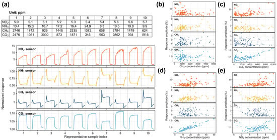
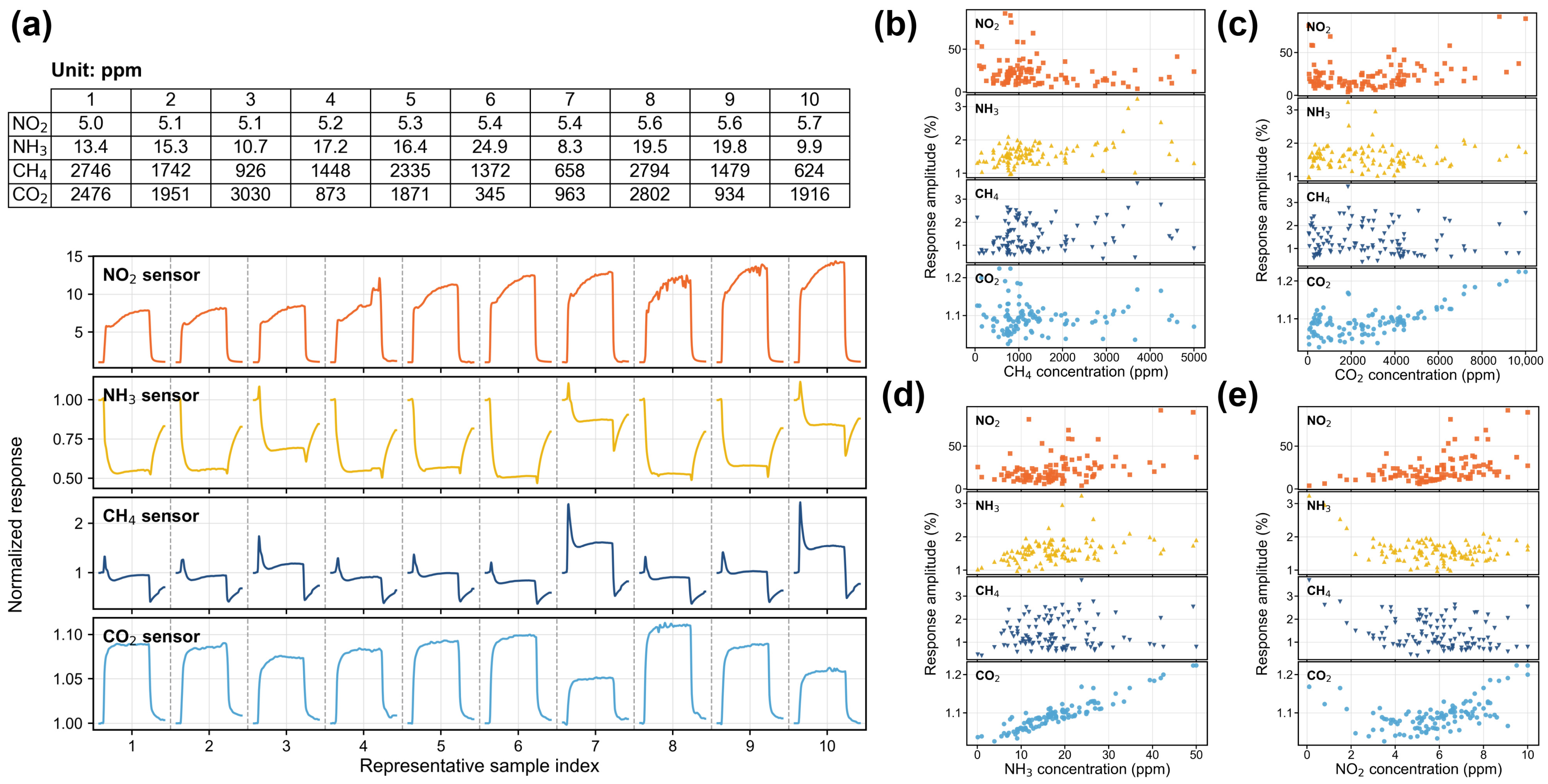
Figure 1 further demonstrates the inherent challenges of mixed-gas quantification. Although our previous work confirmed that the selected gas-sensing materials exhibited good single-gas responses toward their corresponding target gases [29], Figure 1b–e show that their response become strongly coupled under mixed-gas exposure. Representative mixture samples yield distinct response patterns across the four sensing channels, and the response amplitude plots verify that the concentration of a displayed gas component does not correspond to any independent single-channel response. Such cross-response behavior increases the ambiguity of single-channel calibration, but also provides multivariate composition-dependent information at the array level. Therefore, the observed cross-sensitive behavior does not contradict the target-oriented sensor selection; rather, it reveals why the whole-array dynamic response should be modeled for mixed-gas concentration regression. These phenomena reveal that mixed-gas quantification cannot be accurately achieved through independent single-gas calibration schemes or limited steady-state feature descriptors. Therefore, a high-performance deployable model is required to fully exploit cross-channel transient dynamic information while maintaining a compact, lightweight architecture.

Figure 1. Dynamic responses and cross-sensitivity of the four-sensor array under mixed-gas exposure. (a) Normalized responses of the four sensing channels for ten representative gas mixtures. (b–e) Mixed-gas response amplitude correlations of the four channels with CH₄, CO₂, NH₃, and NO₂ concentrations, respectively.

2.2. Calibration Gradient Response Augmentation

Controlled mixed-gas calibration is labor-intensive and time-consuming, while extensive collection of additional concentration combinations may also accelerate sensor aging and degrade device stability. To expand effective calibration coverage, we adopt a response-consistent data augmentation strategy, termed CalibGrad × 6. The core principle is to introduce subtle perturbations to gas concentration labels and update the corresponding sensor response curves along calibration-aware gradient directions learned from real measured samples. In this manner, the augmented responses do not introduce meaningless random noise but strictly conform to the local response variation trends inherent to the sensor array system.

For practical implementation, a ridge-regression calibration model is first fitted to correlate normalized gas concentrations with baseline-referenced response windows. For each measured sample, minor concentration perturbations are sampled within gas-specific constraint ranges. Relatively larger perturbation magnitudes are applied to CH₄ and CO₂, as these two gases exhibit higher normalized prediction errors. The sensor response window is subsequently adjusted according to the learned calibration gradient. Subtle sensor-level variations, including baseline shift, gain jitter, and smooth noise, are further incorporated to simulate realistic minor measurement fluctuations in practical scenarios. The SDRE features are recomputed for all augmented data to ensure feature consistency. The final dataset comprises 110 original samples and 660 augmented samples, resulting in a total of 770 valid samples for model training.

2.3. Sparse Dynamic Response Encoding

Following the calibration dataset expansion, the remaining key challenge lies in effectively encoding sensor response curves while fully preserving the dynamic characteristics illustrated in Figure 1. Rather than relying solely on terminal steady-state response values that discard transient information, the proposed SDRE module characterizes each sensor response curve from three complementary perspectives:

$$\mathcal{D}\left(X,X_0\right)=\left[X,\Delta X,\dot{X}\right],$$

where X is the normalized response, ΔX = X − X₀ is the baseline-referenced response change, and $\dot{X}$ is a smoothed finite-difference curve. The first view preserves the absolute sensor state, the second emphasizes gas-induced resistance change, and the third describes response and recovery kinetics. For four sensors, SDRE yields 12 channels:

$$\mathcal{D}\in {\mathbb{R}}^{T\times 12}.$$

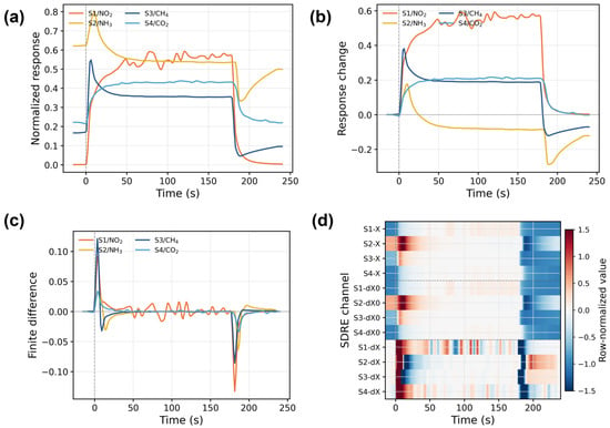
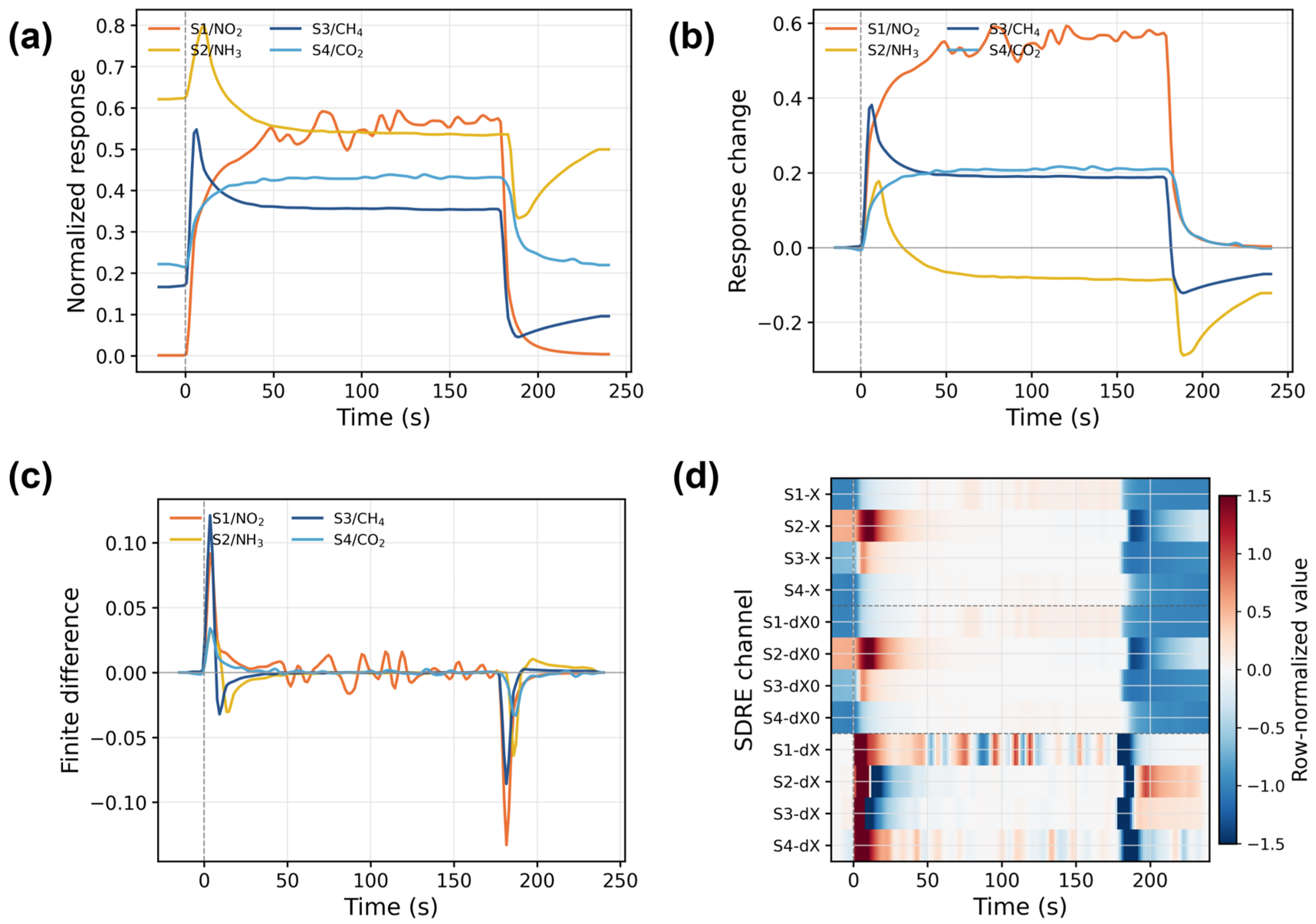
The construction of the SDRE response field is illustrated in Figure 2 using a representative mixed-gas sample. Specifically, Figure 2a–c present the original normalized response, baseline-referenced response change, and smoothed finite-difference response, respectively, while Figure 2d integrates these three response views into the final 12-channel SDRE response field. The original normalized response curves retain the absolute sensor state, the baseline-referenced curves emphasize gas-induced response variations, and the smoothed finite-difference curves highlight response and recovery kinetics. The resulting 12-channel response field provides a compact yet physically interpretable representation of the complete transient sensing process.

Figure 2. Sparse dynamic response encoding of a representative mixed-gas sample. (a) Original normalized responses. (b) Baseline-referenced response changes. (c) Smoothed response differences. (d) 12-channel SDRE response field. Dashed lines indicate gas exposure and recovery boundaries.

2.4. SDRMixer Architecture

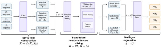
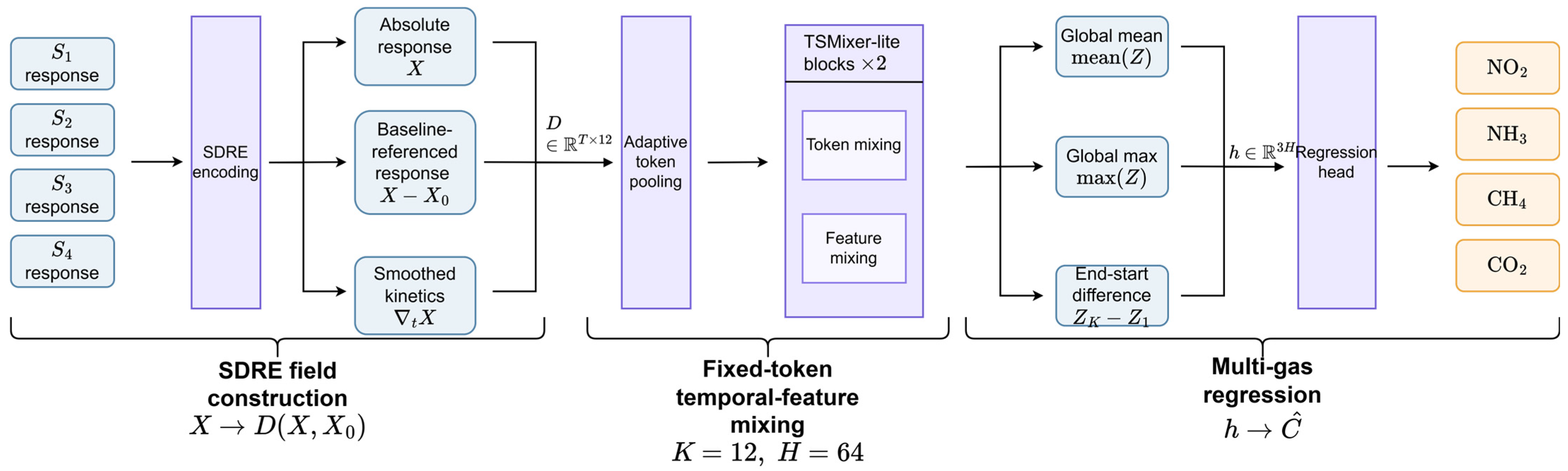
As illustrated in Figure 3, the final modeling step maps the encoded SDRE response field to four target gas concentrations through a compact neural network. SDRMixer first condenses each full-length response curve into 12 fixed response-stage tokens, enabling compact representation of the complete exposure and recovery dynamics within a shortened sequence. Each token is linearly projected into a 64-dimensional hidden space and subsequently processed by two lightweight temporal-feature mixing blocks. These blocks mix information along the response-stage direction and across SDRE channels, allowing the model to use both time-dependent response shape and cross-sensor interaction. The regression head combines the average response state, the strongest response state, and the change between the first and last response-stage tokens to predict the four normalized gas concentrations.

Figure 3. Architecture of SDRMixer for mixed-gas quantification. SDRE response field is tokenized, mixed by lightweight temporal-feature blocks, and mapped to four gas concentrations through a compact regression head.

2.5. Evaluation Protocol

Two evaluation settings were used in this study. The first setting was an augmentation-enriched calibration domain benchmarking protocol based on the CalibGrad ×6 dataset. This setting was used for the SDRE ablation study, gas-wise prediction visualization, and comparisons with lightweight and standard deep learning baselines. In this setting, all compared models were trained and evaluated using the same augmented calibration domain dataset, preprocessing procedure, cross-validation protocol, training schedule, evaluation metrics, and comparable hyperparameter tuning process.

The second setting was an original-measurement-based validation protocol. In this setting, only the 110 experimentally measured mixed-gas samples were used, without CalibGrad-augmented samples. Five-fold cross-validation was performed on the original experimental measurements, and the experiment was repeated with five random seeds to assess result variability. This setting provides an additional conservative assessment of SDRMixer based exclusively on real measured calibration samples.

3. Results

This section evaluates SDRMixer from four perspectives: the contribution of the proposed response encoding, gas-specific prediction performance, accuracy–efficiency trade-off against lightweight and standard deep learning baselines, and additional stability assessment based on original experimental measurements. All compared models were trained and evaluated using the same dataset, preprocessing procedure, cross-validation protocol, training schedule, evaluation metrics, and comparable hyperparameter tuning process. Gas concentration labels were normalized according to the predefined experimental concentration ranges of each gas.

3.1. SDRE Ablation

We further conduct ablation experiments to verify whether performance gains stem from the proposed response encoding scheme or the mixer backbone alone. Table 1 compares the model performance using raw responses, baseline-referenced responses, and complete SDRE features, with the identical lightweight mixer architecture adopted consistently across all groups. Raw-TSMixer achieves a normalized MAE of 0.0224. Incorporating the baseline-referenced response cuts the MAE down to 0.0195. The full SDRE module further lowers the MAE to 0.0181, with the computational cost maintained at merely 1.00 M FLOPs per sample. This validates the first core design principle of our method: explicit decoupling of the absolute sensor response, baseline-referenced excitation signal, and transient kinetic components as independent feature views delivers clear performance improvements. Accordingly, SDRMixer is far more than a generic mixer module naively applied to unprocessed raw sensor time series.

Table 1. Ablation study of SDRE components.

Model	Input Representation	MAE	${\mathit{R}}^2$	Params	FLOPs /Sample
Raw-TSMixer	$X$	0.0224	0.9803	49.1 k	1.38 M
Delta-TSMixer	$\left[X,X-X_0\right]$	0.0195	0.9851	49.4 k	1.39 M
SDRMixer	$\left[X,X-X_0,{\nabla }_{t}X\right]$	0.0181	0.9872	48.7 k	1.00 M

3.2. Task-Level SDRMixer Performance

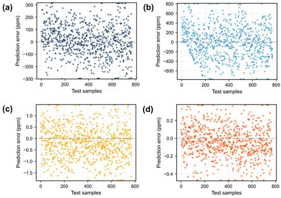
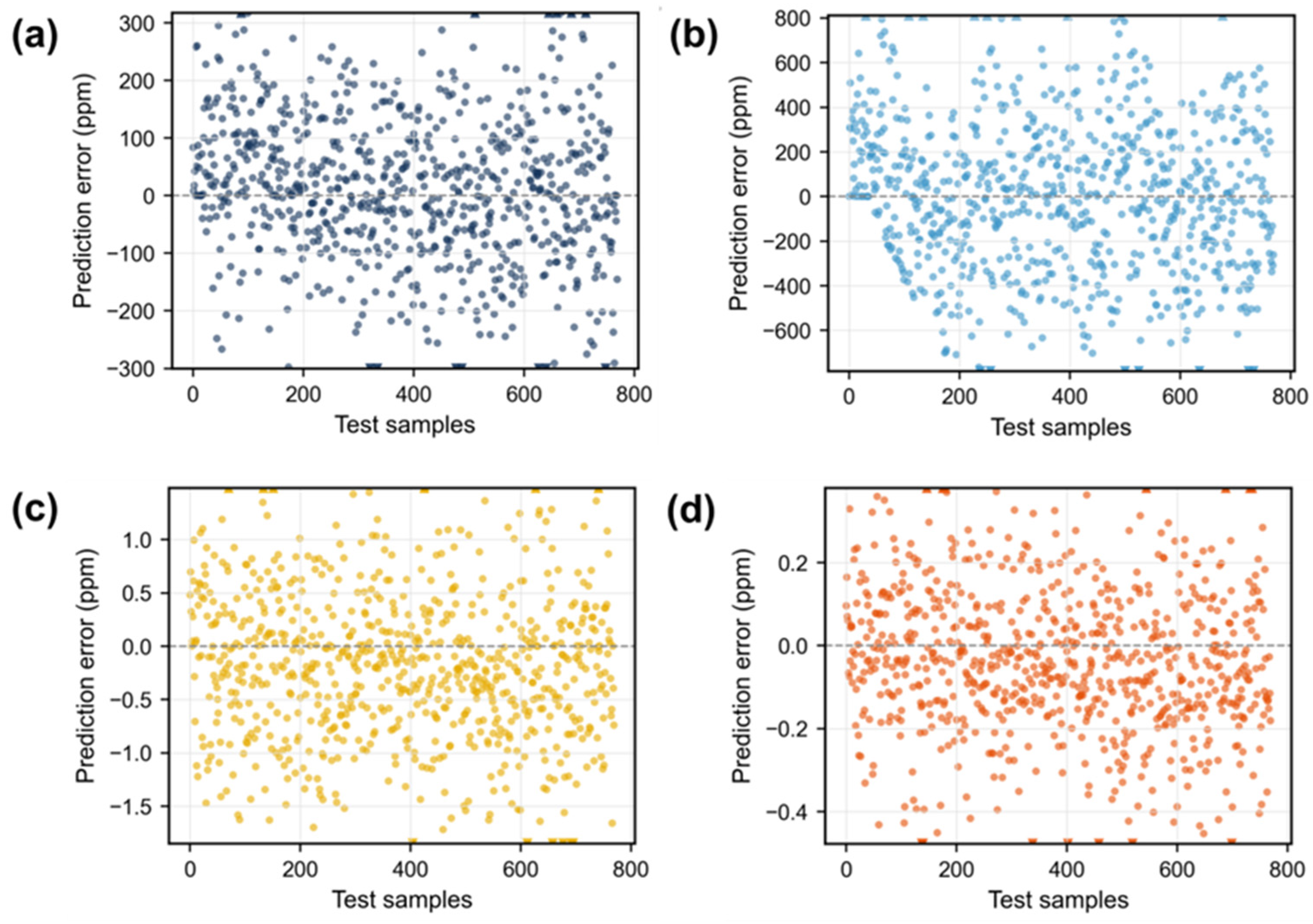
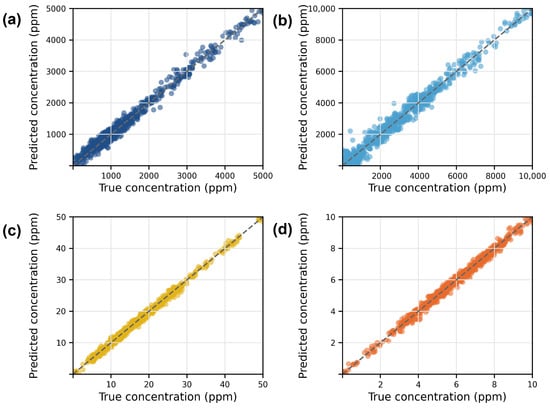
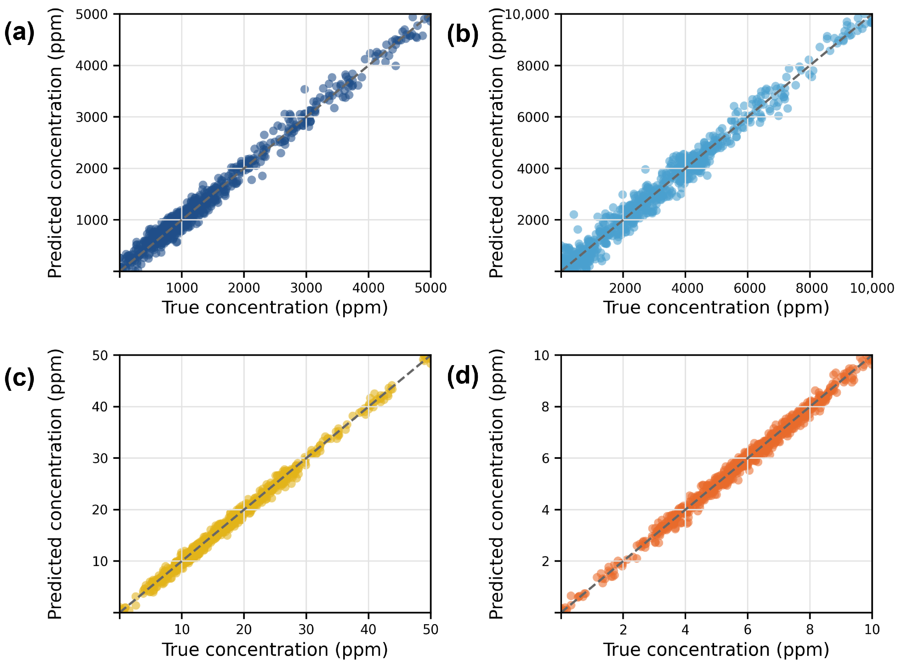
Figure 4 analyzes the physical-unit prediction error distributions of SDRMixer. The signed errors are centered near zero for all four gases, indicating no obvious systematic bias. Figure 5 compares the predicted and measured concentrations in physical units, where the predicted values are generally distributed close to the ideal one-to-one line. In Figure 4 and Figure 5, subplots (a–d) correspond to CH₄, CO₂, NH₃, and NO₂, respectively, allowing the gas-wise prediction error distributions and true-versus-predicted regression results to be compared under their different concentration scales. To provide a scale-aware quantitative summary of the physical-unit errors, Table 2 further reports the gas-specific concentration ranges, MAE, weighted mean absolute percentage error (WMAPE), and R² values.

Figure 4. Physical-unit prediction error distributions of SDRMixer for four gases: (a) CH₄, (b) CO₂, (c) NH₃, and (d) NO₂. The y-axis represents the signed prediction error in ppm, and the dashed horizontal line indicates zero error.

Figure 5. True-versus-predicted concentration plots of SDRMixer for four gases: (a) CH₄, (b) CO₂, (c) NH₃, and (d) NO₂. The dashed diagonal line represents the ideal one-to-one prediction.

Table 2. Gas-specific concentration ranges and physical-unit prediction performance of SDRMixer.

Gas	Range (ppm)	MAE (ppm)	WMAPE (%)	R2
NO2	0.1–10	0.140 ± 0.009	2.38 ± 0.16	0.9912 ± 0.0016
NH3	0.1–50	0.563 ± 0.025	3.11 ± 0.12	0.9941 ± 0.0010
CH4	50.1–5000	98.6 ± 4.8	6.98 ± 0.27	0.9858 ± 0.0016
CO2	52.2–10,000	269.4 ± 16.2	9.19 ± 0.63	0.9772 ± 0.0025

3.3. Comparison with Lightweight Neural Baselines

Table 3 compares SDRMixer with compact sequence models and the literature-style lightweight gas sensor baselines, including the patch-based time series model JointPatchTST [30] and the recurrent neural network baseline Small-long short-term memory (LSTM) [31]. All baseline models adopt resource-efficient architectures tailored for embedded sensing scenarios; however, they rely on either generic sequence learning or compressed handcrafted response summaries, failing to fully exploit the comprehensive SDRE dynamic response field. SDRMixer achieves the lowest normalized MAE across all lightweight comparison schemes. Representative literature-based lightweight models, including Small-LSTM, Plain-1DCNN, and LeNet-GasCNN, maintain low computational complexity but exhibit substantially inferior prediction accuracy. Under a comparable per-sample FLOP budget, SDRMixer significantly outperforms the lightweight LSTM baseline, reducing the normalized MAE from 0.0388 to 0.0181. This result validates the core conclusion of this work: a compact sensing model can deliver superior quantification performance only when its input representation and temporal mixing mechanism are explicitly tailored to the intrinsic dynamic characteristics of gas sensor responses.

Table 3. Comparison with lightweight baselines under the same evaluation setting.

Model	R2	MAE	Params	FLOPs
SDRMixer	0.9872	0.0181	48.7 k	1.00 M
JointPatchTST [30]	0.9803	0.0228	161.0 k	5.70 M
Small-LSTM [31]	0.9304	0.0388	5.0 k	1.11 M
Plain-1DCNN	0.8308	0.0553	3.3 k	0.90 M
LeNet-GasCNN	0.8228	0.0615	2.9 k	0.35 M

3.4. Comparison with Standard Deep Baselines

Table 4 compares SDRMixer with higher-capacity recurrent, temporal-convolutional, attention-based, and Inception-style baselines, including LSTM [31], Inception-lite [32], temporal-convolutional network (TCN) [33], Transformer [34], BiGRU [35] and gated recurrent unit (GRU) [36]. Compared with Inception-lite, SDRMixer reduces the normalized MAE from 0.0191 to 0.0181 while lowering per-sample FLOPs from 51.83 M to 1.00 M. When benchmarked against TCN and Transformer models, SDRMixer achieves comparable or improved prediction accuracy with drastically reduced computational consumption. This outcome suggests that physically structured sensor response representations can reduce the computational burden of downstream learning tasks while maintaining high prediction accuracy within the augmented calibration domain benchmarking setting.

Table 4. Comparison with standard deep baselines under the same evaluation setting.

Model	R2	MAE	Params	FLOPs
SDRMixer	0.9872	0.0181	48.7 k	1.00 M
LSTM [31]	0.9787	0.0232	157.6 k	49.44 M
Inception-lite [32]	0.9859	0.0191	161.8 k	51.83 M
TCN [33]	0.9835	0.0207	110.4 k	36.42 M
Transformer [34]	0.9831	0.0204	230.5 k	48.31 M
BiGRU [35]	0.9749	0.0245	123.8 k	37.19 M
GRU [36]	0.9740	0.0246	123.8 k	37.19 M

3.5. Validation on Original Experimental Measurements

To further evaluate the stability of SDRMixer on real measured calibration samples, additional validation was conducted using only 110 original experimental measurements, without incorporating any CalibGrad-augmented samples. Specifically, five-fold cross-validation was performed on the original experimental dataset, and the entire experiment was repeated with five random seeds to quantify result variability.

As summarized in Table 5, SDRMixer achieves an overall R² of 0.9272 ± 0.0036 and a normalized MAE of 0.0397 ± 0.0024 in this validation scenario based solely on original measurements. In contrast to the benchmark results obtained with augmented calibration data, this validation yields a more conservative evaluation that relies exclusively on real experimental measurements. The gas-specific quantitative results in Table 5 further demonstrate that SDRMixer sustains reliable concentration regression performance for all four target gases on the investigated sensor array dataset.

Table 5. Validation performance of SDRMixer on original experimental measurements.

Gas	Range (ppm)	MAE (ppm)	WMAPE (%)	R2
NO2	0.1–10	0.285 ± 0.055	4.74 ± 0.91	0.9570 ± 0.0129
NH3	0.1–50	1.140 ± 0.122	6.11 ± 0.65	0.9640 ± 0.0080
CH4	50.1–5000	266.1 ± 24.2	19.34 ± 1.76	0.8872 ± 0.0166
CO2	52.2–10,000	529.9 ± 71.2	18.40 ± 2.47	0.9007 ± 0.0273

4. Discussion

The results first confirm that mixed-gas quantification is fundamentally an array-selectivity problem. Figure 1 shows that the response amplitude of an individual channel is not uniquely determined by its nominal target concentration. This phenomenon aligns with the well-recognized sensing mechanisms of chemiresistive gas sensors, in which competitive adsorption, surface chemical reactions, catalytic effects, and heterointerface modulation collectively distort the sensor response to individual gas components [1]. Although orthogonal material engineering can alleviate response correlation across channels, fully decoupled and independent sensing channels are difficult to sustain under varying concentration levels, ambient humidity, and long-term aging interference [4]. Instead of relying on traditional independent single-gas calibration strategies, SDRMixer explicitly models cross-sensitivity as valuable multivariate feature information for accurate mixed-gas quantification.

This perspective also clarifies the relationship between the present SDRMixer framework and our previous LDNN-based study using the same experimental dataset [29]. Although both studies are based on the same four-gas sensor array measurements, the data representation and modeling objective are different. The previous work mainly used compact response descriptors, such as steady-state response values, to construct a local concentration regression model. In contrast, the present work directly uses the complete normalized transient response window, including both the rising and recovery processes, as the model input. This difference allows SDRMixer to exploit richer temporal response information rather than relying only on limited response amplitude features. Moreover, the previous LDNN strategy focused on local response-concentration fitting by selecting highly correlated neighboring samples around each predicted point, whereas SDRMixer learns a reusable lightweight mapping from full response windows to four gas concentrations. Therefore, this work extends the previous local descriptor-based regression framework to full-window dynamic response modeling, enabling unified and deployment-oriented quantification of mixed gases.

SDRE ablation experiments further clarify the benefits of explicit physical response structuring. The baseline raw-TSMixer yields a normalized MAE of 0.0224. Integrating the baseline-referenced response component reduces the MAE to 0.0195, and further embedding the kinetic feature component lowers the error to 0.0181. Previous tapped-delay-based methods have validated the efficacy of temporal response information for ternary mixture estimation, while time series fluctuation features combined with 1D-CNNs have proven effective for binary mixture discrimination [8,14]. Neural regression studies also corroborate that dynamic sensor transient responses carry rich concentration-dependent information [14,15]. Distinct from these data-driven strategies that rely on parameterized feature learning, SDRE decouples absolute response states, gas-induced signal variations, and temporal kinetic characteristics without introducing any trainable parameters. The consistent performance gains observed in ablation studies demonstrate that such physically interpretable multi-view feature decomposition effectively reduces the learning burden of the downstream mixer module. More importantly, the contribution of SDRMixer lies in the coordinated design of dynamic response encoding, response-stage tokenization, and lightweight temporal-feature mixing. This design transforms raw transient sensor curves into compact and physically meaningful response-stage representations, enabling the model to capture baseline states, gas-induced variations, response/recovery kinetics, and cross-channel interactions within a deployment-friendly architecture.

The comparison with existing models also illustrates the trade-off between accuracy and efficiency related to sensors. Classical or shallow electronic-nose regressors are attractive because of their low cost and small-data suitability, but their performance depends strongly on feature engineering [10,13]. Deep mixture models, including 3D-CNN-based regression and general neural mixture-identification systems, can learn richer nonlinear interactions [18,20]. TCN-based concentration prediction further demonstrates the benefit of temporal receptive fields under varying conditions [22]. Notably, the proposed SDRMixer achieves superior quantification accuracy over TCN, Transformer, recurrent networks, and Inception-style baselines, while maintaining an extremely low computational cost of only 1.00 M FLOPs. This insight demonstrates that elaborate pre-structuring of sensor-specific response components prior to temporal and cross-channel feature mixing outweighs the benefits of blindly increasing model capacity.

Compact computational overhead is particularly critical for model deployment on integrated, low-power gas-sensing hardware. Highly integrated electronic noses reduce sensor-system size and power consumption, but an embedded inference model must fit the remaining memory, latency, and energy budget [5]. Although the lightweight CNN and LSTM baselines feature low parameter counts, they suffer from substantially higher prediction errors, demonstrating that simply compressing generic neural architectures cannot achieve reliable high-precision quantification. Differing from naive model shrinking strategies, SDRMixer leverages fixed response-stage tokenization and a lightweight feature mixing backbone, achieving a compact parameter scale of 48.7 k while completely preserving full dynamic response characteristics. This well-balanced design shows potential for edge online sensor nodes compared with purely boosting representation capability by expanding sequence depth or stacking complex attention modules.

The augmentation results should be interpreted in the context of gas sensor calibration rather than as evidence of independent experimental generalization. Random-mixture calibration and optimized calibration schemes aim to cover multicomponent concentration space with fewer measurements [24,25]. Data augmentation and interpolation can further improve coverage and prediction speed, while transfer learning can reduce the calibration required for related MOS sensors [26,27]. Under this setting, the out-of-fold prediction results in Figure 5 demonstrate the ability of SDRMixer to learn concentration-dependent response patterns within the calibrated mixed-gas response space. In addition, the original-measurement-based validation in Section 3.5 provides supporting evidence that SDRMixer can maintain stable regression performance on real measured calibration samples without relying on augmented data. This result further demonstrates the potential of the proposed dynamic response encoding and lightweight temporal-feature mixing strategy. Future work will extend this calibration domain evaluation toward more practical deployment scenarios, including newly prepared gas mixtures, multiple sensor batches, long-term drift, controlled temperature and humidity perturbations, and additional interfering gases.

From the perspective of method applicability, SDRMixer should be regarded as a sensor array response modeling framework rather than a material-specific model restricted to the present In₂O₃-, Pd-ZnO-, Au-SnO₂-, and Pd-LaFeO₃-based channels. The framework itself does not require these exact sensing materials or the same four gas species. Instead, its applicability relies on whether the selected sensor array can provide reproducible, distinguishable, and concentration-dependent transient response patterns within a calibrated gas system. Under this premise, the SDRE module can organize the original response state, baseline-referenced response variation, and response/recovery kinetics, while the lightweight mixer can learn nonlinear cross-channel relationships for multi-output concentration regression. Therefore, SDRMixer may provide a transferable modeling strategy for other partially selective mixed-gas sensor arrays. However, for a new gas system, the sensor array still needs to be selected according to the target gases, experimentally calibrated, and retrained or adapted using the corresponding response data.

Nevertheless, several inherent limitations at the sensor and system levels still need to be addressed. Long-term sensor drift, ambient humidity and temperature fluctuations, gas flow-rate variations, sensor replacement, and unseen interfering gases can substantially shift sensor response distributions. Existing studies on drift compensation and open-set recognition have demonstrated that fixed electronic-nose models generally require periodic adaptive updates for stable performance [28]. Meanwhile, practical turbulent-mixture monitoring further introduces unpredictable variability caused by realistic gas transport dynamics. Although small-sample environmental compensation methods can mitigate partial temperature and humidity interference, they cannot fully eliminate the demand for external field validation. Future work will focus on comprehensive robustness evaluations of SDRMixer under more practical scenarios, including unseen concentration combinations, multiple sensor batches, controlled temperature and humidity perturbations, long-term aging processes, and diverse interfering gas environments. These systematic experiments will further evaluate whether the promising accuracy–efficiency advantage of SDRMixer can be generalized from the investigated calibration dataset to practical long-term deployment applications.

5. Conclusions

This paper presents SDRMixer, a lightweight, sensor-customized framework for mixed-gas concentration quantification within sensor array calibration datasets. The work starts from a practical conflict in gas sensor deployment: mixed-gas responses are nonlinear and cross-sensitive, but measured calibration samples are limited and deployment-oriented models must remain compact. SDRMixer addresses this conflict by constructing an SDRE response field [X, X − X₀, ∇_tX] and applying compact temporal-feature mixing over fixed response-stage tokens. Under the augmentation-enriched calibration domain benchmarking setting, SDRMixer achieves a normalized MAE of 0.0181 and an R² of 0.9872 using only 48.7 k parameters and 1.00 M FLOPs. Comprehensive comparisons against conventional deep architectures, generic lightweight sequence models, and compact gas-sensing models demonstrate that SDRMixer delivers a good balance between accuracy and computational efficiency. In addition, validation on original experimental measurements further supports the stability and potential of SDRMixer on real measured calibration samples. These findings indicate that explicit multi-dimensional dynamic response encoding is an effective modeling strategy for mixed-gas quantification within the investigated calibration domain. The compact parameter count and low computational cost suggest the potential of SDRMixer for deployment-oriented sensor instruments; however, independent validation using newly prepared gas mixtures, multiple sensor batches, long-term drift tests, environmental perturbations, and interfering gases is still required before robust field deployment can be claimed.

References

- Walker, J.; Karnati, P.; Akbar, S.A.; Morris, P.A. Selectivity mechanisms in resistive-type metal oxide heterostructural gas sensors. Sens. Actuators B Chem. 2022, 355, 131242. [Google Scholar] [CrossRef] [Scilit]
- Duan, X.; Jiang, Y.; Liu, B.; Duan, Z.; Zhang, Y.; Yuan, Z.; Tai, H. Enhancing the carbon dioxide sensing performance of LaFeO3 by Co doping. Sens. Actuators B Chem. 2024, 402, 135136. [Google Scholar] [CrossRef] [Scilit]
- Khan, M.A.H.; Thomson, B.; Debnath, R.; Motayed, A.; Rao, M.V. Nanowire-based sensor array for detection of cross-sensitive gases using PCA and machine learning algorithms. IEEE Sens. J. 2020, 20, 6020–6028. [Google Scholar] [CrossRef] [Scilit]
- Pineau, N.J.; Kompalla, J.F.; Güntner, A.T.; Pratsinis, S.E. Orthogonal gas sensor arrays by chemoresistive material design. Microchim. Acta 2018, 185, 563. [Google Scholar] [CrossRef] [Scilit]
- Li, Z.; Yu, J.; Dong, D.; Yao, G.; Wei, G.; He, A.; Wu, H.; Zhu, H.; Huang, Z.; Tang, Z. E-nose based on a high-integrated and low-power metal oxide gas sensor array. Sens. Actuators B Chem. 2023, 380, 133289. [Google Scholar] [CrossRef] [Scilit]
- Yu, Y.; Cao, X.; Li, C.; Zhou, M.; Liu, T.; Liu, J.; Zhang, L. A review of machine learning-assisted gas sensor arrays in medical diagnosis. Biosensors 2025, 15, 548. [Google Scholar] [CrossRef] [Scilit]
- Kumar, V.; Mishra, V.N.; Dwivedi, R.; Das, R.R. Classification and Quantification of Binary Mixtures of Gases/Odors Using Thick-Film Gas Sensor Array Responses. IEEE Sens. J. 2014, 15, 1252–1260. [Google Scholar]
- De Vito, S.; Castaldo, A.; Loffredo, F.; Massera, E.; Polichetti, T.; Nasti, I.; Vacca, P.; Quercia, L.; Di Francia, G. Gas concentration estimation in ternary mixtures with room temperature operating sensor array using tapped delay architectures. Sens. Actuators B Chem. 2007, 124, 309–316. [Google Scholar] [CrossRef] [Scilit]
- Fan, S.; Li, Z.; Xia, K.; Hao, D. Quantitative and qualitative analysis of multicomponent gas using sensor array. Sensors 2019, 19, 3917. [Google Scholar] [CrossRef] [Scilit] [PubMed]
- Ma, H.; Wang, T.; Li, B.; Cao, W.; Zeng, M.; Yang, J.; Su, Y.; Hu, N.; Zhou, Z.; Yang, Z. A low-cost and efficient electronic nose system for quantification of multiple indoor air contaminants utilizing HC and PLSR. Sens. Actuators B Chem. 2022, 350, 130768. [Google Scholar] [CrossRef] [Scilit]
- Javed, U.; Ramaiyan, K.P.; Kreller, C.R.; Brosha, E.L.; Mukundan, R.; Sengupta, A.M.; Morozov, A.V. Quantification of gas concentrations in NO/NO2/C3H8/NH3 mixtures using machine learning. Sens. Actuators B Chem. 2022, 359, 131589. [Google Scholar] [CrossRef] [Scilit]
- Xu, Y.; Meng, R.; Zhao, X. Research on a gas concentration prediction algorithm based on stacking. Sensors 2021, 21, 1597. [Google Scholar] [CrossRef] [Scilit] [PubMed]
- Wang, Y.; Jia, P.; Cui, H.; Peng, X. A novel regression prediction method for electronic nose based on broad learning system. IEEE Sens. J. 2021, 21, 19374–19381. [Google Scholar] [CrossRef] [Scilit]
- Li, X.; Hu, X.; Li, A.; Kometani, R.; Yamada, I.; Sashida, K.; Noma, M.; Nakanishi, K.; Fukuda, Y.; Takemori, T.; et al. Identification of Binary Gases’ Mixtures from Time-Series Resistance Fluctuations: A sensitivity-controllable SnO2 gas sensor-based approach using 1D-CNN. Sens. Actuators A Phy. 2023, 349, 114070. [Google Scholar] [CrossRef] [Scilit]
- Iwata, K.; Abe, H.; Ma, T.; Tadaki, D.; Hirano-Iwata, A.; Kimura, Y.; Suda, S.; Niwano, M. Application of neural network based regression model to gas concentration analysis of TiO2 nanotube-type gas sensors. Sens. Actuators B Chem. 2022, 361, 131732. [Google Scholar] [CrossRef] [Scilit]
- Zhan, C.; He, J.; Pan, M.; Luo, D. Component analysis of gas mixture based on one-dimensional convolutional neural network. Sensors 2021, 21, 347. [Google Scholar] [CrossRef] [Scilit] [PubMed]
- Freddi, S.; Vaghi, L.; Penoni, A.; Scapinello, L.; Sangaletti, L. A minimal electronic nose based on graphene functionalized with metalated pyrazinoporphyrazines and phthalocyanines for ammonia, benzene, and hydrogen sulfide discrimination. Chemosensors 2025, 13, 165. [Google Scholar] [CrossRef] [Scilit]
- Chu, J.; Li, W.; Yang, X.; Wu, Y.; Wang, D.; Yang, A.; Yuan, H.; Wang, X.; Li, Y.; Rong, M. Identification of gas mixtures via sensor array combining with neural networks. Sens. Actuators B Chem. 2021, 329, 129090. [Google Scholar] [CrossRef] [Scilit]
- Zhang, W.; Wang, L.; Chen, J.; Bi, X.; Chen, C.; Zhang, J.; Hans, V. A novel gas recognition and concentration estimation model for an artificial olfactory system with a gas sensor array. IEEE Sens. J. 2021, 21, 18459–18468. [Google Scholar] [CrossRef] [Scilit]
- Pareek, V.; Chaudhury, S.; Singh, S. Hybrid 3DCNN-RBM network for gas mixture concentration estimation with sensor array. IEEE Sens. J. 2021, 21, 24263–24273. [Google Scholar] [CrossRef] [Scilit]
- Li, X.; Guo, J.; Xu, W.; Cao, J. Optimization of the mixed gas detection method based on neural network algorithm. ACS Sens. 2023, 8, 822–828. [Google Scholar] [CrossRef] [Scilit] [PubMed]
- Ni, S.; Jia, P.; Xu, Y.; Zeng, L.; Li, X.; Xu, M. Prediction of CO Concentration in different conditions based on Gaussian-TCN. Sens. Actuators B Chem. 2023, 376, 133010. [Google Scholar] [CrossRef] [Scilit]
- Kang, M.; Cho, I.; Park, J.; Jeong, J.; Lee, K.; Lee, B.; Del Orbe Henriquez, D.; Yoon, K.; Park, I. High accuracy real-time multi-gas identification by a batch-uniform gas sensor array and deep learning algorithm. ACS Sens. 2022, 7, 430–440. [Google Scholar] [CrossRef] [Scilit] [PubMed]
- Baur, T.; Bastuck, M.; Schultealbert, C.; Sauerwald, T.; Schütze, A. Random gas mixtures for efficient gas sensor calibration. J. Sens. Sens. Syst. 2020, 9, 411–424. [Google Scholar] [CrossRef] [Scilit]
- Ma, Y.; Qiu, X.; Duan, Z.; Liu, L.; Li, J.; Wu, Y.; Yuan, Z.; Jiang, Y.; Tai, H. A novel calibration scheme of gas sensor array for a more accurate measurement model of mixed gases. ACS Sens. 2024, 9, 6022–6031. [Google Scholar] [CrossRef] [Scilit] [PubMed]
- Kim, J.; Shin, W.; Hong, S.; Jeong, Y.; Jung, G.; Choi, W.Y.; Kim, J.J.; Park, B.G.; Lee, J.H. A novel pathway to construct gas concentration prediction model in real-world applications: Data augmentation; fast prediction; and interpolation and extrapolation. Sens. Actuators B Chem. 2023, 382, 133533. [Google Scholar] [CrossRef] [Scilit]
- Robin, Y.; Amann, J.; Goodarzi, P.; Schneider, T.; Schütze, A.; Bur, C. Deep learning based calibration time reduction for MOS gas sensors with transfer learning. Atmosphere 2022, 13, 1614. [Google Scholar] [CrossRef] [Scilit]
- Yao, Y.; Chen, B.; Liu, C.; Qu, C. Investigation on the combined model of sensor drift compensation and open-set gas recognition based on electronic nose datasets. Chemom. Intell. Lab. 2023, 242, 105003. [Google Scholar] [CrossRef] [Scilit]
- Li, J.; Ma, Y.; Duan, Z.; Zhang, Y.; Duan, X.; Liu, B.; Yuan, Z.; Wu, Y.; Jiang, Y.; Tai, H. Local dynamic neural network for quantitative analysis of mixed gases. Sens. Actuators B Chem. 2024, 404, 135230. [Google Scholar] [CrossRef] [Scilit]
- Nie, Y.; Nguyen, N.H.; Sinthong, P.; Kalagnanam, J. A time series is worth 64 words: Long-term forecasting with transformers. arXiv 2022, arXiv:2211.14730. [Google Scholar]
- Hochreiter, S. Long short-term memory. Neural Comput. 1997, 9, 1735–1780. [Google Scholar] [CrossRef] [Scilit] [PubMed]
- Ismail Fawaz, H.; Lucas, B.; Forestier, G.; Pelletier, C.; Schmidt, D.F.; Weber, J.; Webb, G.I.; Idoumghar, L.; Muller, P.A.; Petitjean, F. Inceptiontime: Finding alexnet for time series classification. Data Min. Knowl. Disc. 2020, 34, 1936–1962. [Google Scholar] [CrossRef] [Scilit]
- Bai, S.; Kolter, J.Z.; Koltun, V. An empirical evaluation of generic convolutional and recurrent networks for sequence modeling. arXiv 2018, arXiv:1803.01271. [Google Scholar]
- Vaswani, A.; Shazeer, N.; Parmar, N.; Uszkoreit, J.; Jones, L.; Gomez, A.N.; Kaiser, Ł.; Polosukhin, I. Attention is all you need. Adv. Neural Inf. Process. Syst. 2017, 30, 5998–6008. [Google Scholar]
- Schuster, M.; Paliwal, K.K. Bidirectional recurrent neural networks. IEEE T. Signal Proces. 1997, 45, 2673–2681. [Google Scholar] [CrossRef] [Scilit]
- Cho, K.; Van Merriënboer, B.; Gulçehre, Ç.; Bahdanau, D.; Bougares, F.; Schwenk, H.; Bengio, Y. Learning phrase representations using RNN encoder-decoder for statistical machine translation. In Proceedings of the 2014 Conference on Empirical Methods in Natural Language Processing (EMNLP); Association for Computational Linguistics: Stroudsburg, PA, USA, 2014; pp. 1724–1734. [Google Scholar]
Disclaimer/Publisher’s Note: The statements, opinions and data contained in all publications are solely those of the individual author(s) and contributor(s) and not of MDPI and/or the editor(s). MDPI and/or the editor(s) disclaim responsibility for any injury to people or property resulting from any ideas, methods, instructions or products referred to in the content. |
© 2026 by the authors. Licensee MDPI, Basel, Switzerland. This article is an open access article distributed under the terms and conditions of the Creative Commons Attribution (CC BY) license.