


Abstract
Near-infrared spectroscopy supports rapid quantification of moisture, oil, protein, and starch in corn. Their prediction models may require different spectral inputs, complicating shared-variable selection. We developed the multicomponent shared wavelength selection (MCSWS) algorithm to select one fixed-size subset for all four constituents. It combines a scale-normalized objective with five adaptively fused descriptors. Evaluation used 80 corn samples originally measured at Cargill and distributed by Eigenvector Research, with 700 wavelengths from the m5 instrument. Eight repeated four-way splits assessed held-out prediction (outer cross-validation). Selection and calibration tuning used training-only five-way splits (inner cross-validation). MCSWS retained 38 variables, a 94.6% reduction, and achieved a joint normalized root-mean-square error of prediction (JNRMSEP) of 0.35 ± 0.03. Rounded results were 0.34 ± 0.02 for full-spectrum partial least squares (PLS) regression and competitive adaptive reweighted sampling coupled with PLS (CARS-PLS). Values are means ± sample standard deviations across eight repeat means. After exploratory corn calibration development, the frozen workflow yielded JNRMSEP = 0.049 using six variables on the official casein–glucose–lactate (CGL) test split versus 0.047 for CARS-PLS and 0.016 for full-spectrum PLS. These results characterize an accuracy–dimensionality trade-off. Variable reduction concerns regression inputs after full-spectrum preprocessing, not demonstrated reductions in physical measurements.
1. Introduction
Near-infrared spectroscopy (NIRS) provides a rapid and non-destructive approach to food composition analysis by measuring overtone and combination absorptions associated mainly with hydrogen-containing functional groups [1,2]. It has been widely applied to quality evaluation of agricultural products, pharmaceutical analysis, and industrial process monitoring [1,2,3]. Recent reviews have further identified the combination of NIRS and chemometrics as an important platform for rapid food-quality assessment [2,3]. However, near-infrared absorption bands are broad, strongly overlapped, and sensitive to matrix scattering, temperature, and sample physical state. Quantitative analysis, therefore, generally depends on multivariate calibration rather than isolated spectral channels [1,4].
The primary study uses the publicly available corn spectroscopy dataset distributed by Eigenvector Research, referred to here as the corn benchmark; its provenance and composition are documented in Section 2.1. In this study, a component is a constituent quantified in corn: moisture, oil, protein, or starch. Its reference content is a response variable, the quantity to be predicted from the spectra. Multicomponent analysis, therefore, means predicting these four constituent contents, not extracting four latent variables from a regression model. The analytical task is to quantify all four constituents from the measured near-infrared (NIR) spectra. These constituents contribute differently to overlapping NIR bands: moisture is associated with water O–H absorptions, oil with lipid C–H contributions, protein with N–H and amide contributions, and starch with carbohydrate O–H and C–H contributions [1,2]. Their concentration ranges, response variances, and spectral signal strengths can also differ. Consequently, wavelengths informative for predicting one constituent need not be equally informative for the others.
Partial least squares (PLS) regression is widely used for near-infrared calibration because its latent variables, weighted combinations of spectral variables, can accommodate high-dimensional and strongly collinear spectra [5]. Full-spectrum PLS retains all measured spectral variables, which can include redundant or weakly informative regions [6,7]. Numerical wavelength selection reduces the variables supplied to a calibration model without changing the original acquisition [6,7]. Its relevance to instrument design is conditional: a smaller regression input set can support fewer physical measurements only if the required features can be computed from those measurements [6,8,9,10]. Restricting physical spectral coverage may also limit analyses of additional constituents or new sample matrices; instrument simplification therefore requires task-specific acquisition and preprocessing validation [9,10]. The present study evaluates model input reduction using full-spectrum data rather than a reduced-channel instrument. Numerical wavelength-selection algorithms pursue this model-input reduction in different ways [7]. Regression- and stability-based numerical methods rank variables according to their contribution to a calibration model, whereas numerical competitive-shrinkage and population-search algorithms progressively remove weak variables from the search space [7,11,12]. Other approaches, including spatial projection and bootstrap-based hybrid search, attempt to reduce spectral redundancy or combine complementary measures of wavelength importance [13,14]. These methods have demonstrated that compact subsets can retain substantial predictive information [6,7].
Many of these numerical wavelength-selection algorithms were developed or commonly applied with a single response as the selection target [7,8]. Applying such single-response selection procedures independently to several constituents can produce different wavelength sets for different responses, increasing the total number of distinct spectral variables used across the constituent-specific calibration models [8].
Shared wavelength selection means selecting one set of spectral-variable indices for use by all constituent-specific calibration models. It introduces an additional optimization problem: retaining information for several responses within one limited input-variable set [8]. Differences in constituent concentration ranges and response variances also need to be accounted for when responses are combined [15,16]. Directly combining component errors on their original scales can cause high-variance responses to dominate the selection objective. Conversely, independently optimizing each response does not guarantee a compact set that is jointly informative [8,17]. Covariance selection (CovSel) provides a direct multi-response alternative by selecting variables according to their joint covariance with the response matrix and orthogonally removing information associated with previously selected variables [8]. However, the practical value of an adaptive multi-index strategy must be established through a matched comparison under the same model input variable budget and validation splits. A further concern is information leakage: if component weights, preprocessing choices, wavelength subsets, or model complexity are optimized using test responses, the reported prediction error can be optimistically biased [18,19,20].
Recent developments extend wavelength selection beyond conventional coefficient ranking. Zhang et al. introduced neural network-based variable importance combined with iterative variable elimination [21], while Pamukçu coupled genetic algorithm search with hybrid regression for high-dimensional, small-sample NIR data [22]. In multi-response analysis, the covariance-oriented variable-clustering method g-CovSel extends covariance selection to complementary groups of correlated variables [23]. A 2026 review also places variable selection alongside nonlinear modeling, portable instrumentation, and calibration-transfer challenges in food analysis [24]. More specifically, a genetic algorithm (GA) incorporating maximum-relevance minimum-redundancy (mRMR) filtering, termed GA-mRMR, refines wavelength subsets within genetic algorithm iterations and determines subset size from data [25]. Recent competitive adaptive reweighted sampling (CARS) developments include Calibrated CARS (CCARS), which couples wavelength selection with partial least squares discriminant analysis (PLS-DA) calibration and evaluates model robustness through permutation tests and learning curves in lettuce classification [26].
These advances distinguish several optimization targets: relevance–redundancy-guided subset search [25], classification-specific calibration [26], and complementary variable-group selection [23]. The present study addresses multi-response regression under a prespecified input-variable budget defined as the number of distinct spectral variables retained for all constituent-specific models. The selection objective combines normalized validation errors across constituents, and the selected subset has a fixed cardinality, meaning that it contains exactly the prespecified number of variables. The matched CARS, successive projections algorithm (SPA), Monte Carlo uninformative variable elimination (MCUVE), and CovSel comparisons assess this formulation under common validation splits and sparse-variable budgets, separating the selection procedure from subsequent component-specific calibration.
Cross-validation estimates prediction error by rotating sample groups, called folds, between model fitting and validation. In nested cross-validation, outer-training samples are used for model development, while a separate outer-test group is reserved for evaluation; the inner folds divide only the outer-training samples for selection and tuning. A current partition is the sample group associated with the particular split being analyzed.
Here, we propose the multicomponent shared wavelength selection (MCSWS) algorithm to identify one fixed-size spectral-variable subset for simultaneous prediction of the target constituent contents. The same input-variable indices are shared across the constituent-specific calibration models. Within each training partition, prediction difficulty is defined operationally as the full-spectrum single-response PLS (PLS1) cross-validation error divided by the standard deviation of that constituent’s reference values. A larger normalized error indicates a larger prediction error relative to the observed response variation under the specified calibration protocol. This quantity describes model-based prediction difficulty, not the intrinsic chemical complexity of a constituent. These normalized errors are converted to non-negative component weights that sum to one; the weights determine each constituent’s contribution to the joint validation objective. Candidate subsets are evaluated with constituent-specific errors normalized by the same training-response standard deviations. Five complementary wavelength-evaluation scores (descriptors), comprising regression contribution, elite frequency, bootstrap stability, group impact, and non-redundancy, are then normalized and adaptively fused according to their associations with candidate-subset performance. The resulting scores update wavelength-sampling probabilities while the active set is progressively reduced to the prespecified model input variable budget.
Algorithm evaluation separated wavelength selection from subsequent component-specific calibration. Prediction errors were assessed by repeated nested cross-validation, with every data-dependent decision restricted to the corresponding outer-training data [18,19,20]. MCSWS was compared with full-spectrum PLS, CARS-PLS, SPA-PLS, MCUVE-PLS, and the multi-response CovSel-PLS method under matched validation conditions [8,11,12,13]. Equal component weighting was included as a control for the proposed difficulty-weighting scheme, and leave-one-descriptor-out analyses were used to examine the contribution of the five-descriptor formulation without redefining the algorithm after observing the results. Model-input-budget sensitivity was evaluated exploratorily around the prespecified primary budget.
The empirical evaluation used the corn benchmark introduced above as the primary dataset and the official casein–glucose–lactate (CGL) calibration–test split to evaluate the frozen calibration rule. Dataset composition, sample counts, acquisition information, and split definitions are described in Section 2.1.
The main contributions of this work are as follows:
(1) A dimensionless multi-response selection criterion is formulated using training-derived response standard deviations and component-specific cross-validation errors. This formulation prevents the numerical scale of a constituent from directly determining its contribution to the joint objective.
(2) A fixed-budget shared wavelength-selection procedure is developed by adaptively combining five wavelength descriptors. The method returns one shared spectral-variable set for all target constituents rather than merging independently selected component-specific subsets.
(3) A leakage-controlled experimental framework is used to compare MCSWS with both single-response-derived sparse methods and the multi-response CovSel baseline. Component weighting, wavelength selection, preprocessing decisions, and latent-variable tuning are confined to training data.
(4) A guarded component-specific PLS1 calibration module is evaluated only after the wavelength set has been locked. Because this calibration refinement was developed during the corn analysis, its corn results are treated as exploratory, and the complete rule was frozen before access to the official CGL test responses.
Accordingly, MCSWS is intended for multicomponent NIR calibration in which several constituent-specific models must use the same fixed-size set of spectral inputs. Its practical role is to coordinate variable selection across the constituents under a common input budget, allowing the trade-off between prediction error and input dimensionality to be assessed within one shared-variable framework. The corn and CGL benchmarks illustrate this use for four-component compositional analysis. The shared inputs are extracted after full-spectrum preprocessing.
2. Materials and Methods
2.1. Datasets, Spectral Measurements, and Preprocessing
The public corn benchmark was originally acquired at Cargill (headquarters: Wayzata, MN, USA) and distributed by Eigenvector Research (Manson, WA, USA) [27]. The corn dataset contained 80 samples measured at 700 wavelengths from 1100 to 2498 nm at 2 nm intervals. Four reference constituents were analyzed: moisture, oil, protein, and starch. Only the m5spec.data spectra were used; spectra from other instruments were not combined with this dataset. The response distributions are summarized in Table 1. The same benchmark is described by Poerio and Brown as Cargill cornmeal samples measured in reflectance on instruments designated m5, mp5, and mp6 [28]. These designations identify the archived instruments rather than verified manufacturer/model specifications. This study used the m5 records and did not perform new spectrometric acquisition or reference assays. Cultivar, cultivation site, grinding particle size, manufacturer/model, acquisition temperature, detailed optical geometry, scan averaging, and constituent-specific reference-assay protocols are not provided in the public archive. The numerical spectral signal was used as supplied without reconstructing or converting its optical representation.
Table 1.
Descriptive statistics of the four reference constituents in the corn dataset.
In the MAT-file archive corn.mat, m5spec is the DataSet object containing spectra from instrument m5, and its data field, accessed as m5spec.data, is the 80 × 700 numerical matrix used as X. Each row represents one sample and each column one wavelength. The corresponding 80 × 4 propvals.data matrix supplies the reference property values in the documented order moisture, oil, protein, and starch [27]. These supplied labels, rather than spectral peak identification, define the four prediction targets.
For the corn analysis, the practical task was to predict four reference constituent contents from each measured spectrum. Water O–H groups contribute moisture-sensitive overtone and combination bands around 1450 and 1940 nm. Oil contains aliphatic C–H groups, including CH2 and CH3 groups, with overtone and combination responses broadly around 1700 and 2300 nm. Protein contributes N–H and amide-related combination bands, including mixed N–H and C=O contributions around 2150–2200 nm. Starch is a polysaccharide containing hydroxyl O–H, C–H, and C–O/C–O–C groups; its carbohydrate-related responses overlap those of water and other constituents [1,2]. These assignments provide broad chemical context rather than unique identification of a constituent at one wavelength. Calibration uses the combined spectral variation to predict known reference contents, not to identify unknown compounds from isolated peaks. Prediction accuracy is assessed against held-out reference values. Table 1 summarizes those reference values, and Figure 1a,b shows the measured corn NIR spectra before and after the reference preprocessing.
Figure 1.
Mean corn NIR spectra before and after the prespecified reference preprocessing. Solid curves show the mean across 80 m5 spectra; shaded bands show ±1 between-sample SD at each wavelength calculated with an n − 1 denominator. Panel (a) shows the archived signal as supplied; panel (b) shows SG1(11,2) + SNV spectra. The inset in (b) plots the SD itself on a separate, labeled ordinate because its magnitude is small relative to the mean spectrum. The main-panel SD band is not enlarged. This spread describes variation among samples, not repeated-scan uncertainty or a confidence interval.
For the matched primary comparison, spectra were preprocessed using a Savitzky–Golay first derivative with an 11-point window and a second-order polynomial, followed by row-wise standard normal variate transformation, denoted as SG1(11,2) + SNV. These fixed transformations were applied separately to each complete spectrum; SG used interpolation at the spectral boundaries, and SNV used the mean and population standard deviation of that sample’s 700 derivative values. They did not estimate parameters across samples. Figure 1a,b provides a descriptive visualization of the raw and preprocessed corn NIR spectra; this visualization used all 80 spectra and was not used to estimate predictive performance. This pipeline served as a common fixed reference for wavelength selection and the primary method comparison; the reported primary experiment did not include a preprocessing pre-screen to establish it as optimal. First differentiation suppresses constant spectral offsets, while SNV standardizes each transformed spectrum by its own mean and standard deviation. The 11-point, second-order SG setting specifies local polynomial smoothing and differentiation, not a universally optimal spectral bandwidth. Alternative windows, derivative orders, and SNV inclusion were compared subsequently within training-only calibration grids (Section 2.4 and Section 2.7.5) after the selected variables had been locked.
Subsequent processing comprised training-derived response standardization for PLS2 selection, shared-variable selection, and constituent-specific PLS1 calibration with internal variable scaling disabled. PLS models performed mean centering within each model fit. After the shared subset was locked, component-specific latent variables were tuned by inner CV, and the resulting models were evaluated on held-out outer-test samples. Exploratory preprocessing-grid and guarded-calibration analyses are described separately in Section 2.4 and Section 2.7.5. Spectral processing and model calibration did not create or replace the archived reference-property values.
The casein–glucose–lactate (CGL) dataset is a separate NIR chemical-mixture benchmark, not a subset of corn. The distributor attributes it to Tormod Naes and Tomas Isaksson and describes a full three-component mixture design with reference responses for casein, glucose, lactate, and moisture (wt%) [27]. Casein, glucose, and lactate are the three designed mixture constituents; moisture is an additional recorded response. The dataset contains 231 samples and 117 wavelengths spanning 1104–2495 nm. Its official split of 153 calibration samples and 78 test samples was retained without modification, with six selected variables for each sparse method. CGL evaluates the frozen algorithm and calibration rule on different response chemistry. Its weights, selected variables, and fitted regression models are estimated from its own calibration samples; corn concentrations or fitted model coefficients are not transferred to CGL.
2.2. Problem Definition
For corn, each of eight repetitions divided the 80 samples into four outer folds. One 20-sample fold was reserved for evaluation (the outer-test fold), and the remaining 60 samples formed the current outer-training partition. Five-fold inner cross-validation divided those 60 training samples into five groups of 12. Each inner split fitted a candidate model on 48 samples (the inner-training partition) and evaluated it on the remaining 12 (the inner-validation fold), rotating the validation group through all five folds. Inner-validation predictions guided selection and tuning; outer-test responses were used only after the corresponding model-development decisions were locked.
Partial least squares (PLS) regression provides the calibration basis for relating high-dimensional spectral measurements to physicochemical responses [5].
PLS1/PLS2 modeling and response centering and scaling follow established PLS practice [29]. Cross-validation-based model selection follows the nested-validation principles described in [18,19,20].
Let denote the preprocessed spectral matrix in the current training partition, where n is the number of training samples and p is the number of full-spectrum wavelength variables. The corresponding response matrix is .
For the complete corn benchmark, the spectral data form an 80 × 700 matrix: each row contains the spectrum of one sample, and each column corresponds to one wavelength. The associated response matrix has 80 rows and four columns, ordered as moisture, oil, protein, and starch. A response row therefore contains the four reference contents of the same sample as the corresponding spectral row. In each outer-training partition, X and Y have dimensions 60 × 700 and 60 × 4, respectively. After wavelength selection, the model input matrix has dimensions 60 × 38, while Y retains its four response columns. Each individual spectrum is a one-dimensional sequence; stacking sample spectra produces the two-dimensional sample-by-wavelength matrix used here, not a three-dimensional spectral array.
For the corn dataset, K = 4, corresponding to moisture, oil, protein, and starch. The integer index k = 1, 2, 3, or 4 identifies the corresponding response column, in that order. Common wavelength-selection methods are frequently applied to each response separately, which can produce different component-specific wavelength subsets [5,6]. Such separate selections can enlarge the union of variables used across component models. MCSWS therefore searches for one shared subset that is used to calibrate all K responses. Here, shared denotes a common input-variable index set, not a requirement that every selected variable be informative for every response or that the variables occupy one contiguous absorption region. The set can include variables from distinct, non-overlapping regions. Subsequent PLS1 models are fitted separately for each component, allowing response-specific regression coefficients and latent-variable counts.
Equations (1)–(3) define the difficulty-based prioritization, weighted normalized validation objective, and fixed-cardinality selection problem used in MCSWS. They combine established prediction-error and response-scaling operations with the study-specific weighting rule; they are not presented as new definitions of RMSE or standard deviation.
Because the four responses have different numerical ranges and dispersions, their raw prediction errors cannot be combined directly. For component k, a full-spectrum PLS1 model was first evaluated by five-fold inner cross-validation within the current outer-training partition. Its normalized prediction difficulty and component weight were defined as
where is the minimum root-mean-square error of cross-validation (RMSECV) across the admissible latent-variable counts of the full-spectrum PLS1 model for component k, and is the sample standard deviation of yk in the current outer-training partition. Consequently, .
Inner-cross-validation error is calculated from predictions for samples withheld from the corresponding inner model fit. In five-fold inner CV, each training sample is predicted once by a model fitted on the other four folds, and all held-out residuals are pooled to calculate RMSECV. It is ordinary root-mean-square error (RMSE) applied to cross-validated predictions, expressed in the original response units; dividing it by the training-response standard deviation gives the dimensionless difficulty in Equation (1). Here, “minimum” refers to the latent-variable search, not to selecting the best fold. Appendix A.3 provides the explicit calculation [18,20,29].
Prediction difficulty is an operational, model- and protocol-dependent measure of estimating a constituent’s content from spectra. A larger error-to-SD ratio denotes greater prediction error relative to that response’s observed dispersion; it does not describe an intrinsic property of the chemical constituent. The component weighting is the study-specific prioritization rule in Equation (1).
The number of latent variables in each full-spectrum PLS1 model was selected from 1 to 15 by five-fold inner cross-validation. If two latent-variable counts produced exactly the same minimum error, the smaller value was retained.
For a candidate wavelength subset S, its dimensionless joint cross-validation error was defined as
where is the component-specific inner-cross-validation error obtained from the shared multi-response PLS selection model using subset S. The wavelength-selection problem was, therefore, formulated as
The superscript asterisk in Equation (3) denotes the solution sought by the fixed-cardinality optimization, not multiplication or statistical significance. The arg min operator returns a minimizing subset, whereas min returns the objective value. MCSWS approximates this optimization by selecting the lowest-error terminal candidate from its sampled population as specified in Equation (A15).
The equality constraint fixes the number of selected preprocessed spectral variables supplied to the regression models. It is a model input constraint, not a physical measurement-channel constraint. The primary corn analysis used , corresponding to a 94.6% reduction from the original 700 wavelengths. The equal-component control used , whereas the difficulty-weighted version used training-derived component weights.
The reported analyses used q = 38 for corn and q = 6 for CGL, with the same q imposed on the sparse comparators within each dataset. These values define the fixed-cardinality comparisons reported here; they are not validated hardware configurations or evidence of an optimal physical channel count. The exploratory corn analysis at q = 20, 38, and 60 assesses sensitivity to input dimensionality and does not establish a hardware optimum.
2.3. Algorithm Workflow
MCSWS approximates the fixed-budget optimization problem defined in Equation (3) through an iterative population-based search comprising spectral preprocessing, training-only initialization, candidate-subset evaluation, five-descriptor calculation, adaptive descriptor fusion, and active-set shrinkage (Figure 2).
Figure 2.
Overall workflow of MCSWS. The downward arrow from PLS2 inner-CV evaluation ranks candidate subsets to form the elite pool. A separate arrow leaves the right side of the same PLS2 block and carries the negative joint inner-CV error of each candidate to the descriptor–performance correlation step. This is training-only feedback, not a second model fit. Colored cells schematically distinguish spectral variables; they do not encode a quantitative color scale.
Each complete spectrum was first processed using a Savitzky–Golay first derivative with an 11-point window and a second-order polynomial, followed by row-wise standard normal variate normalization, denoted as SG1(11,2) + SNV. For corn, SG processing was applied along the 700-point spectrum spanning 1100–2498 nm; SNV then used the mean and standard deviation of all 700 derivative values in that sample. For CGL, the same selection-stage preprocessing was applied along all 117 recorded wavelengths, and SNV used all 117 derivative values in that sample. Variable selection was performed after these transformations. SG values depend on neighboring spectral samples, whereas the SNV statistics in this implementation depend on the complete transformed spectrum. Thus, selecting 38 or six output variables does not reduce the raw spectral acquisition required by the evaluated workflow. These fixed transformations are sample-wise and do not fit preprocessing parameters using other samples or test responses.
Within each outer-training partition, the response variables were standardized as
where and were calculated only from the current outer-training partition.
In Equation (4), denotes the standardized response, whereas denotes the original reference concentration for sample i and component k. The symbol “:=” means “is defined as”; this equation defines a transformation rather than an identity or an iterative update. The training mean and sample standard deviation are fixed within the corresponding outer fold. The original reference concentrations remain unchanged, and the standardized responses are used in the PLS2 wavelength-selection model [29].
A single latent-variable count was selected for the multi-response PLS2 model used during wavelength searching. Let , where is the minimum number of samples in an inner-training partition. The selection-stage latent-variable count was
Thus, was selected once from the full spectrum within each outer-training partition and was subsequently fixed during candidate-subset searching. For a subset whose cardinality was smaller than , the effective number of latent variables was limited by the subset dimension and the available inner-training samples.
The initial active wavelength set and sampling probabilities were defined as . The active-set size followed a prespecified geometric schedule. At iteration t, the target subset size was
Exponential variable-retention schedules are used in CARS [11]. Equation (6), repeated in Equation (A12), specifies the geometric schedule adopted here, with its endpoint fixed by the declared variable budget, where T = 7 was the fixed number of MCSWS iterations.
At each iteration, W = 14 candidate subsets were sampled independently from At−1 according to the current probabilities . Sampling was performed without replacement within each candidate subset, ensuring that every candidate contained exactly unique wavelengths. Each subset was evaluated using the fixed selection-stage PLS2 model and the joint criterion in Equation (2). The candidate subsets were ranked in ascending order of , and the lowest-error 15% formed the elite pool , with a minimum of two elite subsets. In the implementation, the elite count was the larger of two and round (0.15 × W); with W = 14, the two lowest-error candidates were retained at every iteration.
The descriptor formulation combines established coefficient-magnitude ranking [11], coefficient-stability ranking in UVE-type selection [12], and bootstrap resampling [30] with the MCSWS population statistics and multi-response aggregations. Equation (7) summarizes the five operational descriptors, which are expanded in Equations (A1)–(A5).
Five descriptors were then calculated for every wavelength :
Here, is the component-weighted absolute PLS coefficient contribution averaged over the elite subsets; is the elite inclusion frequency; and is the bootstrap coefficient-stability ratio. Six bootstrap resamples were used, each containing 80% of the outer-training samples drawn with replacement. Operationally, each bootstrap score was the component-weighted sum of absolute coefficients from one PLS2 fit on the current active set; the mean and sample SD of these scores across the six resamples defined S (Equation (A3)). The quantity measures the relative difference between the mean candidate error when wavelength is absent, , and when it is present, . If either candidate group was empty, was set to zero. Finally, measures non-redundancy through the mean absolute Pearson correlation between wavelength and the remaining wavelengths in the current active set. For the stability descriptor in Equation (7), the coefficient-score SD is taken across the six bootstrap resamples, not across search iterations; Equation (A3) gives the fully indexed computation.
Min–max normalization and Pearson correlation follow standard data-processing definitions [31]; their use in Equations (8), (9), (A5)–(A7) and (A9) is specified for the current active set and candidate population.
Each descriptor was independently transformed to the interval [0,1] by min–max normalization. A descriptor with zero range was assigned a normalized score of zero. Let denote the normalized score of wavelength for descriptor . The candidate-level mean descriptor score was calculated as
The association between descriptor m and candidate performance was then quantified as
Softmax is the established normalized exponential mapping [32]. MCSWS applies it to descriptor–performance correlations and wavelength scores to obtain adaptive fusion weights and sampling probabilities; these applications are specified in Equations (10) and (12).
Negative, undefined, or constant-score correlations were assigned a value of zero. The descriptor-fusion weights and composite wavelength scores were subsequently calculated as
where . This fusion is performance-guided rather than unsupervised, because its weights are determined by correlations with inner-cross-validation performance.
The wavelengths in the current active set were ranked by , and the highest-scoring wavelengths were retained:
The sampling probabilities for the next iteration were updated by
where , while wavelengths removed from received zero probability.
When the geometric schedule reached , all candidate subsets contained exactly unique wavelengths. The candidate with the lowest inner at this terminal fixed-budget stage was returned as . This finite stochastic search does not guarantee a global optimum.
After had been locked, separate PLS1 calibration models were fitted for moisture, oil, protein, and starch. Their latent-variable counts were selected independently from 1 to 15 by five-fold inner cross-validation, with the smaller model retained in the case of an exact tie. No outer-test sample or response was used to estimate component weights, select latent variables, calculate descriptors, update sampling probabilities, or determine the final wavelength subset.
2.4. PLS Modeling and Internal Cross-Validation
PLS modeling served three distinct purposes in MCSWS: estimating component difficulty, evaluating candidate wavelength subsets, and constructing the final component-specific calibration models. PLS1 was used for single-component calibration, whereas PLS2 was used to evaluate the four standardized responses jointly during wavelength selection. Internal variable scaling was disabled in all PLS models (scale = false), because spectral preprocessing and response standardization were performed explicitly.
Within each outer-training partition, separate full-spectrum PLS1 models were first optimized for moisture, oil, protein, and starch. The same five inner folds were used throughout the corresponding outer fold. For component k, the admissible latent-variable set and the full-spectrum latent-variable count were defined as
where is the minimum number of samples in an inner-training partition. The smaller latent-variable count was selected when two candidates produced exactly the same RMSECV.
The error from predictions made while each sample was withheld from its inner model fit (out-of-fold error) obtained using was used to calculate the normalized component difficulty dk and weight wk defined in Equation (1). The response standard deviation was calculated from the current outer-training partition using the sample standard deviation. Consequently, the weights were recomputed independently in every outer fold, and then held fixed throughout its wavelength-search iterations.
Difficulty weighting should be interpreted as a training-derived prioritization rule rather than an assumed performance advantage. A larger value of dk gives greater influence to a response with a larger full-spectrum RMSECV relative to its concentration dispersion. The equal-component ablation replaced the selection weights with wk = 1/K while retaining the same outer and inner partitions, selection-stage latent-variable count, and random-number stream. For comparability, its outer JNRMSEP was calculated using the same fold-specific evaluation weights as the other methods.
For candidate-subset evaluation, the outer-training responses were standardized using the means and standard deviations defined in Equation (4). A single PLS2 latent-variable count was then selected once on the full spectrum by minimizing the joint inner-validation criterion in Equation (2) as specified in Equation (5). This value was fixed while all candidate wavelength subsets in the corresponding outer fold were compared. Therefore, candidate ranking was not confounded by performing a separate latent-variable search for every randomly generated subset. When necessary, the effective latent-variable count was capped by the candidate-subset dimension and the minimum inner-training sample size.
For candidate subset , five-fold out-of-fold predictions were generated using the fixed selection-stage PLS2 model. The component-specific errors were normalized by and combined through in Equation (2). A smaller indicated better joint inner-validation performance. This criterion was used only for candidate ranking and wavelength selection; no outer-test response contributed to its calculation. Equivalently, PLS2 predicted responses standardized once by the current outer-training means and SDs; the RMSE on this scale equals the original-unit RMSE divided by the same training SD, and no second SD division was applied.
After the shared wavelength subset had been locked, separate PLS1 models were constructed for the responses. In the matched primary comparison, the wavelength-selection preprocessing, SG1(11,2) + SNV, was retained. The component-specific latent-variable count was selected as
The selected PLS1 model was subsequently refitted using the complete outer-training partition and evaluated once on the corresponding outer-test fold.
A separate guarded component-specific calibration analysis was conducted after inspection of the corn development results and was, therefore, treated as post-specified for corn. This calibration step did not alter the previously selected shared wavelengths. For each response, a reference model was selected from seven preprocessing candidates: SG1(11,2) + SNV, raw spectra, SNV, SG0(11,2) + SNV, SG1(7,2) + SNV, SG1(15,2) + SNV, and SG2(11,2) + SNV. The reference latent-variable range was 1–15.
The expanded calibration grid added SG0(7,2) + SNV, SG0(15,2) + SNV, SG1(9,2) + SNV, SG1(21,2) + SNV, SG2(7,2) + SNV, SG2(15,2) + SNV, SG0(11,2), SG1(11,2), SG2(11,2), and detrending followed by SNV. Its latent-variable limit was increased to 25. In both grids, the effective upper limit was .
Let and denote the minimum inner RMSECV values obtained from the reference and expanded grids, respectively. The expanded calibration was accepted only when it reduced inner RMSECV by at least 2%: ,
Exact ties were resolved according to the declared preprocessing order and then in favor of the smaller latent-variable count. The complete guarded-calibration rule, including the candidate transformations, latent-variable limits, tie-breaking rule, and 2% acceptance threshold, was frozen before the official CGL test responses were evaluated.
The finite latent-variable ranges and tie-breaking conventions in Equations (5), (13), and (14) specify this implementation of CV-based PLS tuning [18,19,29]. The 2% acceptance criterion in Equation (15) is a study-specific calibration rule.
For guarded calibration, each candidate transformation was likewise computed from the complete recorded spectrum before the locked variable indices were extracted. The raw-spectrum candidate is an identity transformation; SNV-containing candidates use the full transformed spectrum, and SG candidates use their specified local spectral windows. The selected-variable count, therefore, describes regression input dimensionality and does not, by itself, specify a physically implementable measurement configuration.
At every stage, component weights, response-standardization parameters, latent-variable counts, preprocessing choices, and shared wavelengths were determined using training data only [18,19,20]. Outer-test responses were accessed only after the wavelength subset and all component-specific calibration decisions had been locked.
2.5. Overview of Wavelength-Evaluation Descriptors
The five descriptors summarized in Equation (7) quantify regression contribution (B), recurrence in elite subsets (F), bootstrap coefficient stability (S), candidate-group error association (I), and spectral non-redundancy (D). They are calculated for wavelengths in the current active set using only the outer-training samples and their inner-validation predictions. Their fully indexed definitions, coefficient aggregation, and numerical conventions are provided in Appendix A.1, Equations (A1)–(A5).
This formulation combines established coefficient-ranking, stability, bootstrap, and correlation tools [11,12,30,31] with the multi-response aggregation used in MCSWS. The complete algorithm retains all five descriptors; the leave-one-descriptor-out comparisons described in Section 2.7.4 assess their contribution without redefining the primary algorithm.
2.6. Overview of Adaptive Fusion and Active-Set Shrinkage
Each descriptor is rescaled to [0,1] within the current active set. The candidate-level mean descriptor score is related to negative joint inner-validation error through Pearson correlation, as summarized in Equations (8) and (9). Negative or undefined correlations are assigned zero. Standard Softmax [32], with fusion sharpness 4, converts these associations into weights for the composite wavelength score in Equation (10).
The highest-scoring wavelengths are retained according to the geometric schedule and ranking rules in Equations (6) and (11). The sampling Softmax in Equation (12), with sharpness 5, guides the next candidate population. Sampling is without replacement within each subset. At the terminal variable budget, the sampled candidate with the lowest joint inner-validation error is returned. Appendix A.2, Equations (A6)–(A15), provides the expanded normalization, fusion, shrinkage, sampling, and terminal-selection definitions. All steps remain confined to the current outer-training partition.
2.7. Experimental Design and Parameter Settings
The experimental evidence was organized into three distinct levels. First, the primary comparison of wavelength-selection methods was conducted on the corn dataset using a prespecified nested cross-validation protocol. Second, model-input-budget sensitivity, descriptor ablation, and guarded calibration refinement were examined as exploratory analyses on corn. Third, the calibration rule developed during the corn analysis was frozen and evaluated on the official calibration–test split of the CGL dataset. This separation was maintained throughout the analysis to distinguish prespecified performance estimates from post-specified development results and frozen external validation.
2.7.1. Nested Validation and Leakage Control
Predictive performance on corn was estimated using eight repeated four-fold outer cross-validations, producing 32 outer training–test splits. Each split contained 60 training samples and 20 test samples. Within every outer-training partition, five-fold inner cross-validation was used for all data-dependent decisions, including component-weight estimation, wavelength selection, preprocessing selection where applicable, and latent-variable tuning.
The outer-test responses were inaccessible during all selection and tuning procedures. They were evaluated only after the wavelength subset, preprocessing rule, component weights, and PLS hyperparameters had been locked. The overall random seed was fixed at 20260715, and deterministic seeds were derived for each repeat, fold, and method.
For each constituent indexed by k, the prediction-difficulty score for estimating its content was calculated exclusively from the current outer-training partition:
where is the sample standard deviation of the corresponding response in the outer-training partition. The normalized difficulty weights were then calculated as
These fold-specific weights were used consistently to evaluate all methods within the same outer split. For the equal-component-weight variant, was used during wavelength selection, while its outer-test JNRMSEP was evaluated using the same fold-specific difficulty weights as the other methods to preserve comparability.
The primary MCSWS configuration was fixed before the 32-fold run: T = 7 shrinkage iterations, W = 14 candidate subsets per iteration, elite fraction 0.15, six bootstrap resamples at an 80% row ratio, descriptor-fusion sharpness γα = 4, sampling-probability sharpness γp = 5, and q = 38 unique wavelengths (Table 2). The primary budget fixes the number of model input variables for the reported corn comparison; it is not an instrument-channel specification. These are explicit fixed computational-budget settings rather than hyperparameter values established as predictive optima. T determines the number of stages in the geometric shrinkage schedule, whereas W determines the candidate population used for performance feedback. The configuration entails 98 candidate-subset evaluations per search and retains two elite candidates per stage under the stated rounding and minimum-size rule. No formal sensitivity sweep of T, W, the bootstrap count, or the Softmax coefficients was conducted. The same search settings were retained on CGL, with q changed to six for the separate fixed-input-budget comparison. This provides a transfer check of one frozen configuration across two datasets rather than evidence that these numerical settings are optimal for other sample sizes or spectral resolutions.
Table 2.
Parameter settings of MCSWS in the corn experiments.
All selectors and final PLS models were trained independently within each outer-training partition. Full-spectrum and component-specific final PLS1 latent variables were selected from 1 to 15 by five-fold inner cross-validation, with the lower count breaking exact ties. The same outer splits and metric definition were used for all methods. Corn was evaluated using eight repeated four-fold outer cross-validations; descriptive summaries used eight repeat-level means, each obtained by averaging the four outer-fold results. These repetitions reused the same 80 samples and were not independent experimental replications. No individual favorable split was selected for reporting, and every completed fold was retained. The recorded software environment for the primary corn analysis was Windows 11 with Python 3.12.13, NumPy 2.3.5, SciPy 1.16.3, pandas 3.0.1, scikit-learn 1.7.2, and Matplotlib 3.10.8.
2.7.2. Compared Methods and Fixed Parameter Settings
The primary corn comparison included full-spectrum PLS, CARS-PLS, SPA-PLS, MCUVE-PLS, CovSel-PLS, difficulty-weighted MCSWS-PLS, and equal-component-weight MCSWS-PLS. Full-spectrum PLS used all 700 wavelengths, whereas every sparse method was constrained to exactly 38 unique wavelengths. The 38-variable setting was fixed for the reported performance comparison. It defines a common model input budget for the sparse methods and is not interpreted as a validated instrument constraint or a globally optimal variable count.
Because CARS and MCUVE are commonly formulated for a single response, they were implemented here as explicit shared-response adaptations. Within each outer-training partition, the four responses were centered and divided by their training standard deviations, and the training-derived difficulty weights were used to aggregate response-specific quantities. For CARS, absolute PLS2 coefficients were combined across responses by a weighted sum. Five restarts were performed, each with 12 exponentially decreasing retention steps. At each step, 80% of the outer-training samples were drawn without replacement, and adaptive reweighted sampling used a Softmax coefficient of 4. The exact-q candidate with the lowest five-fold inner-CV JNRMSECV was retained.
For MCUVE, 30 bootstrap samples, each containing 80% of the outer-training observations sampled with replacement, were fitted using PLS2. For each response and variable, stability was calculated as the absolute mean bootstrap coefficient divided by its bootstrap standard deviation. The response-specific stability vectors were min–max normalized, combined using the same training-derived difficulty weights, and ranked to retain the top q unique variables. SPA was response-free, and therefore, required no response-wise aggregation. It used deterministic QR-like successive projection on the mean-centered outer-training spectra: selection started from the variable with the largest column norm, and each subsequent variable maximized the residual norm after projection onto the variables already selected. The procedure stopped when q unique variables had been retained.
For CARS, MCUVE, and MCSWS, the PLS2 latent-variable count used during selection was chosen by five-fold inner cross-validation and was restricted by the subset dimension and inner-training sample size. Randomized CARS and MCUVE runs used deterministic seeds derived from the fixed base seed (20260715) and the outer repeat and fold. All selection, response standardization, weighting, and tuning were confined to the corresponding outer-training partition. The fixed budgets were q = 38 for corn and q = 6 for CGL. These implementations should, therefore, be interpreted as controlled, fixed-budget multi-response adaptations rather than as unchanged single-response reference algorithms.
For CovSel, responses were standardized within the current outer-training partition. At each selection step, the variable maximizing was retained, after which both X and Y were orthogonally deflated with respect to that variable. CovSel therefore provided a direct equal-response multivariate baseline and did not use the MCSWS difficulty weights.
MCSWS used seven shrinkage iterations and generated 14 candidate subsets per iteration. The elite pool comprised the lowest-error 15% of candidates, subject to a minimum of two candidates. Six bootstrap resamples, each containing 80% of the current training samples, were used for stability estimation. The descriptor-fusion and wavelength-sampling Softmax coefficients were fixed at 4 and 5, respectively.
During candidate-subset evaluation, a PLS2 model was used with the latent-variable count determined by five-fold inner cross-validation. The maximum number of latent variables was 15 and was additionally restricted by the subset dimension and inner-training sample size. After the shared subset had been locked, separate PLS1 models were fitted for individual components, with their latent-variable counts independently selected from 1 to 15. PLS models were fitted without automatic predictor scaling.
2.7.3. Performance Metrics and Statistical Analysis
RMSECV and RMSEP have the same units as the reference response: for corn contents recorded in percent, errors are expressed in percentage points. Component errors divided by the training-response SD, and their joint normalized errors, are dimensionless and non-negative, with no upper bound of one. An individual normalized error below one is smaller than that response’s SD; a joint value below one expresses this relation in the weighted aggregate, not necessarily for every response. Neither is a percentage error relative to constituent content. Component weights and descriptor-fusion weights are different quantities: each is a dimensionless share between zero and one, and each set sums to one.
RMSEP, the coefficient of determination, and deviation-to-error ratios are established calibration-evaluation quantities [29,33]. Equation (18) states the exact conventions used here: the test-response mean is used in the coefficient of determination, and the outer-training response SD is used in the RPD numerator. Equations (16) and (17) restate the difficulty and weighting definitions in Equation (1).
Component-level predictive performance was evaluated using RMSEP, the test coefficient of determination , and the ratio of performance to deviation:
Equation (19) is the outer-test counterpart of the study-defined joint objective in Equation (2), using the same training-derived scaling and weights.
The primary multicomponent metric was the joint normalized RMSEP:
This formulation removes the direct effect of different response scales while retaining the training-derived component weights. The wavelength reduction was reported as
Equation (20) is the arithmetic percentage reduction in regression input variables rather than a new statistical metric.
For corn, the four outer-fold JNRMSEP values were first averaged within each repetition, yielding eight repeat-level means per method. Performance is summarized by the mean and sample standard deviation (SD, calculated with a denominator of seven) across these eight repeat means. All completed folds and repetitions were retained; no favorable run was selected for reporting.
The SD describes variation across repeated data partitions and stochastic algorithm runs on the fixed set of 80 corn samples. It is not a standard error or a confidence interval for performance in a new sample population. The eight repetitions and 32 outer folds do not constitute independent experimental replications; averaging within a repetition does not remove dependence arising from reuse of the samples.
Between-method comparisons of the corn cross-validation results are descriptive. No inferential p-values or confidence intervals are reported for these repeated-CV comparisons, and differences in observed mean error are not interpreted as evidence of statistical superiority or equivalence. The nested validation design separates model selection from outer-test evaluation but does not turn repeated partitions of the same samples into independent validation datasets. Generalization beyond the sampled corn data requires independent external validation on new corn samples.
2.7.4. Exploratory Sensitivity and Descriptor Ablation
Two exploratory analyses were conducted using the same 32 outer splits. First, the effect of the model input variable budget was examined at q = 20, 38, and 60 for CARS, CovSel, and MCSWS. The prespecified 38-variable result remained the primary analysis; the 20- and 60-variable results were not used to redefine the primary budget. These results are summarized descriptively by the mean and sample SD across the eight repeat means without inferential confidence intervals or hypothesis tests. This analysis addresses sensitivity to model input dimensionality, and the descriptor ablations assess the formulation; neither constitutes sensitivity analysis of the fixed search hyperparameters.
Second, five leave-one-descriptor-out MCSWS variants were evaluated at q = 38: MCSWS-minus-B, MCSWS-minus-F, MCSWS-minus-S, MCSWS-minus-I, and MCSWS-minus-D. Each variant used the same outer splits and matched random-number streams as the complete five-descriptor model. The ablation analysis was not used to modify the reported primary algorithm retrospectively. In particular, an ablated model outperforming the complete model was interpreted as evidence of descriptor redundancy or adverse interaction on corn rather than as justification for replacing the prespecified MCSWS definition.
2.7.5. Post-Specified Guarded Calibration Analysis on Corn
After completion of the prespecified corn analysis, a component-specific guarded calibration procedure was investigated to determine whether final PLS1 calibration could be improved without altering the selected shared wavelength subset. This analysis was post-specified and is, therefore, reported as exploratory development evidence.
For each component, a reference calibration grid included SG1(11,2) + SNV, raw spectra, SNV, SG0(11,2) + SNV, SG1(7,2) + SNV, SG1(15,2) + SNV, and SG2(11,2) + SNV, with up to 15 latent variables. The expanded grid added alternative Savitzky–Golay windows and derivative orders, selected no-SNV transformations, and detrending followed by SNV, with up to 25 latent variables.
The expanded calibration replaced the reference calibration only when it reduced inner RMSECV by at least 2%. Otherwise, the reference model was retained. Exact ties were resolved by the predefined candidate order and then by the lower latent-variable count. All guard decisions were based exclusively on outer-training data. Cross-fitted corn prediction plots from this analysis were used as descriptive visualizations and were not treated as a separate independent test set.
To distinguish the effects of preprocessing-grid expansion, the PLS1 latent-variable limit, and the guard, five calibration variants were evaluated on the same locked 38-variable subset in each corn outer fold, using identical outer and inner splits: the original seven-candidate grid with 1–15 latent variables (reference); the original grid with 1–25 latent variables; the expanded 17-candidate grid with 1–15 latent variables and no guard; the expanded grid with 1–25 latent variables and no guard; and the expanded grid with 1–25 latent variables and the 2% guard. The last two variants differed only in the acceptance rule, so their paired descriptive results isolate the observed effect of applying the guard within this analysis.
A fixed-seed oil-label permutation was additionally used as a negative-control diagnostic. Because only one prespecified permutation was performed, this analysis was not interpreted as a formal permutation test.
2.7.6. Frozen External Validation on CGL
The guarded calibration specification was developed after inspecting the corn development results. On CGL, all preprocessing choices, selected wavelengths, latent-variable counts, and guard decisions were determined using only the 153 calibration samples. The locked models were subsequently evaluated once on the 78 official test samples.
Sparse methods retained exactly six unique wavelengths, whereas full-spectrum PLS used all 117 wavelengths. No hypothesis test was performed for the official CGL split because it provided only one calibration–test partition. Consequently, the CGL results are reported using component-level metrics, JNRMSEP, and relative differences between methods without significance claims. This validation was intended to assess whether the frozen MCSWS workflow remained usable under a strict six-variable constraint, not to demonstrate superiority over full-spectrum calibration.
3. Results
3.1. Component Prediction Difficulty and Weight Allocation
For the illustrative full-data fit, full-spectrum five-fold RMSECV values were 0.1418, 0.0450, 0.0961, and 0.1770 percentage points for moisture, oil, protein, and starch, respectively (Table 3). Their reference-content ranges were 9.38–10.99%, 3.09–3.83%, 7.65–9.71%, and 62.83–66.47%, respectively (Table 1). After division by the corresponding response standard deviations, the dimensionless prediction-difficulty scores were 0.3728, 0.2543, 0.1927, and 0.2156, yielding dimensionless component weights of 0.3600, 0.2456, 0.1861, and 0.2082. For starch, 0.2156 means that its full-spectrum cross-validation RMSE was approximately 21.6% of its reference-content SD, not 21.6% of its starch content. These normalized errors are not constrained to [0,1]; the component weights are shares summing to one. Thus, moisture—not starch—received the largest scale-normalized weight. In the nested analysis, all four weights were recomputed separately within each outer-training fold.
Table 3.
Full-spectrum inner-CV errors and scale-normalized component weights for the illustrative full-data fit. RMSECV is in percentage points; component weights are dimensionless shares summing to one.
3.2. Determination of the Historical Best Subset During MCSWS Iterative Selection
Figure 3 presents the illustrative full-data search trace used to define an illustrative variable set; it is not an outer-test performance estimate. Across seven steps, the active set decreased from 700 to 462, 304, 201, 132, 87, 58, and finally, 38 wavelengths. The dimensionless best-candidate JNRMSECV declined from 0.3030 to 0.2519, while the dimensionless candidate median declined from 0.3101 to 0.2642.
Figure 3.
MCSWS shrinkage trajectory and inner-validation error during the full-data illustrative fit. JNRMSECV is dimensionless and uses response-SD normalization; it is not constrained to [0,1]. (a) Number of active wavelengths retained after each shrinkage iteration. (b) Median and best candidate JNRMSECV values across the candidate population at each iteration.
3.3. Adaptive Indicator Weights and Component Error Evolution
To analyze the roles of different variable-evaluation indicators during MCSWS search, the fusion weights of the five indicators were recorded over the iterations. The results are shown in Figure 4.
Figure 4.
Dimensionless adaptive fusion weights of five MCSWS descriptors during full-data search.
In the illustrative trace, group impact I received the largest dimensionless adaptive fusion weight at every iteration (0.489–0.809, equivalent to 48.9–80.9% of the total fusion weight; Figure 4). This means that within-search presence–absence contrasts were strongly associated with candidate performance; it does not establish that I improves held-out performance.
The dimensionless, response-SD-normalized RMSECV trends of the four constituents during MCSWS iteration were also examined, as shown in Figure 5.
Figure 5.
Dimensionless RMSECV/response-SD per component during MCSWS search.
The dimensionless normalized moisture error decreased from 0.3829 to 0.3013 across the trace (Figure 5). Oil and protein ended at 0.2086 and 0.2042, whereas starch followed a nonmonotonic path and ended at 0.2431. Each value is RMSECV divided by that response’s SD in the full-data illustrative fit; for example, 0.3013 represents 30.13% of the moisture-reference SD. Values below one describe the observed error relative to the response dispersion, not a universal performance threshold or a bound imposed by normalization. These curves describe the best candidate within each full-data iteration and should not be interpreted as outer-test estimates.
The leave-one-descriptor-out analysis provides a stricter diagnostic than the adaptive trajectory weights. Omitting I lowered repeat-level mean JNRMSEP from 0.3536 to 0.3331, a descriptive 5.81% reduction (Supplementary Figure S2 and Table S4). Therefore, the five descriptors did not all make a positive held-out contribution in this dataset. The complete five-descriptor MCSWS definition was, nevertheless, retained as the prespecified primary algorithm rather than being altered after seeing the ablation.
3.4. Shared Wavelength Distribution
The distribution of the final MCSWS shared wavelength set on the preprocessed mean spectrum was visualized, as shown in Figure 6.
Figure 6.
Selected preprocessed-variable positions and outer-CV selection frequencies. The 38-variable set is an illustrative full-data fit, not a physical channel configuration; any channel terminology within the plotted legend refers only to selected model input variables. (a) The 38 wavelengths from the illustrative full-data fit overlaid on the mean SG1(11,2) + SNV spectrum. (b) MCSWS wavelength-selection frequency across all 32 outer-training fits. The illustrative variable set and outer-CV stability profile serve different purposes and are, therefore, reported separately.
Figure 6 separates an illustrative full-data variable set from resampling stability. Panel (a) shows the 38 selected preprocessed-variable positions obtained from a fit to all 80 samples. Panel (b) reports exact-position selection frequency across the 32 outer-training fits. The highest individual frequency was 13/32 (40.6%), and five positions in the illustrative full dataset were not selected in any outer fit. These results indicate limited exact-position stability; the full dataset is not presented as a uniquely reproducible wavelength panel or used to estimate predictive performance.
The constituent-related functional groups and overlapping NIR bands are introduced in Section 2.1. Figure 6 places the selected positions in this broad chemical context: coverage around water O–H, lipid C–H, and protein–carbohydrate combination-band regions is consistent with selecting information across several constituents. The selected positions fall within broad NIR regions commonly associated with these constituents; this alignment provides chemical context, not evidence of constituent-specific selectivity.
As explained in Section 2.1, the overlapping bands require a region-level interpretation. The distribution in Figure 6 is, therefore, interpreted jointly rather than through one-to-one assignments of wavelengths to constituents. Figure 6 therefore provides a descriptive, region-level interpretation of the shared variable set. The predictive value of the selection procedure is evaluated separately using held-out outer-test folds in Section 3.6. The illustrative 38-variable set spans 1102–2350 nm and contains both local groupings and widely separated positions. MCSWS optimizes prediction under an input-variable budget without imposing wavelength clustering or filter-bandwidth constraints. Its selected positions, therefore, do not specify a 38-filter instrument. Practical and economic feasibility would require joint evaluation of band placement, bandwidth and transmission, source and detector coverage, optical layout, and signal-to-noise performance; variable count alone does not quantify hardware savings.
3.5. Calibration-Grid and Guard Analyses on Corn
Within each outer fold, MCSWS selected its 38 variables using the 60 outer-training samples only. The five calibration variants described in Section 2.7.5 were then fitted using the same locked variable subset and outer-training data and evaluated on the same untouched 20-sample outer-test fold. Every sample, therefore, received eight outer-test predictions per variant, one from each repeat. Across the 32 outer fits, all 32 selected 38-variable subsets were distinct; no single subset was fixed across repeats.
Under matched splits and locked variable subsets, repeat-level JNRMSEP was 0.207330 ± 0.015783 for the reference grid with, at most, 15 latent variables; 0.190501 ± 0.020182 for the reference grid with, at most, 25; 0.127121 ± 0.009238 for the expanded grid with, at most, 15 and no guard; 0.121153 ± 0.009043 for the expanded grid with, at most, 25 and no guard; and 0.121065 ± 0.009155 for the same expanded grid with the 2% guard. Thus, most of the observed improvement relative to the reference grid accompanied the expansion of preprocessing choices. Holding the expanded grid and 25-latent-variable limit fixed, applying the guard changed the mean JNRMSEP by only 0.000088. It accepted the expanded model in 120 of 128 outer-fold-by-response decisions and retained the reference model in eight. These post-specified corn comparisons are descriptive and do not establish a general benefit of the guard.
For Figure 7, RMSEP and R2 were calculated from the 80 unaveraged outer-test predictions in each repeat, pooling its four test folds before averaging the eight repeat-level scores. The guarded workflow yielded mean pooled outer-test R2 values of 0.9945, 0.9894, 0.9602, and 0.9825 for moisture, oil, protein, and starch, respectively. These repeated-CV estimates come from the same corn dataset and are not independent external-test results.
Figure 7.
Exploratory comparison of reference adaptive calibration and the guarded expanded-grid workflow on corn. (a) Pooled outer-test RMSEP (mean and SD across eight repeats). (b) Pooled outer-test R2 (mean and SD across eight repeats) for the reference adaptive and guarded expanded-grid calibrations.
Figure 8 displays reference constituent content (%) against mean cross-fitted predicted content (%) for moisture (a), oil (b), protein (c), and starch (d). Each of the 80 points represents one sample, with its eight outer-test predictions averaged. Error bars are ±one sample SD across those eight predictions, expressed in percentage points; they are not confidence intervals. Dashed lines indicate identity (predicted = reference), not fitted regressions. The predictions came from different outer-training fits and selected subsets, rather than one fitted 38-variable model or a physical 38-channel instrument. The unaveraged outer-test scores in Figure 7 and the primary matched-calibration comparison remain the basis for interpreting predictive performance.
Figure 8.
Descriptive cross-fitted corn constituent contents (%) under guarded expanded-grid calibration. (a) Moisture; (b) oil; (c) protein; (d) starch.
The corn calibration experiment shows that substantial improvements can be obtained after a shared variable set is locked by allowing component-specific preprocessing and latent-variable choices under nested inner CV. However, the exploratory status of the expanded corn grid requires confirmation under a frozen protocol.
3.6. Comprehensive Comparison with Other Wavelength-Selection Methods
The primary selector comparison used matched fixed SG1(11,2) + SNV calibration for full-spectrum PLS, CARS-PLS, SPA-PLS, MCUVE-PLS, CovSel-PLS, MCSWS-PLS, and MCSWS with equal component weights. All sparse methods retained exactly 38 unique wavelengths in every outer fold. Figure 9 summarizes component-level normalized errors, whereas Table 4 and Figure 10 report repeat-level joint results.
Figure 9.
Component-level prediction error under matched fixed calibration.
Table 4.
Descriptive comparison of corn prediction performance under matched fixed calibration.
Figure 10.
Repeat-level prediction errors under matched fixed calibration on corn. Each circle represents the mean JNRMSEP of four outer-test folds within one repeat; diamonds indicate the arithmetic mean of eight repeat means. All methods use the same eight repeated four-fold splits, five-fold inner validation, and fixed SG1(11,2) + SNV calibration. Sparse methods retain 38 model input variables, and full-spectrum PLS uses 700 (Table 4). The horizontal axis is dimensionless JNRMSEP normalized using outer-training response SDs and weights; lower values indicate lower error. The vertical axis lists methods and is categorical, not a numerical measurement. Orange highlights MCSWS, blue its equal-weight variant, and gray the comparators. Repetitions reuse the same 80 samples; no inferential intervals or significance markers are shown. Abbreviations are defined in Table 4. Variable counts are reported in Table 4. Figure 10 adds the repeat-level distribution, with each method occupying one categorical row and no vertical displacement of its points.
Across the eight repeated outer validations, five-descriptor MCSWS achieved JNRMSEP = 0.3536 ± 0.0270 (mean ± sample SD of eight repeat means; Table 4). The corresponding values were 0.3395 ± 0.0167 for CARS-PLS, 0.3431 ± 0.0221 for full-spectrum PLS, 0.3806 ± 0.0179 for SPA-PLS, 0.3816 ± 0.0292 for CovSel-PLS, and 0.4128 ± 0.0205 for MCUVE-PLS. These descriptive results characterize the observed prediction errors under the matched calibration protocol; they do not establish statistical superiority or equivalence. The equal-component MCSWS variant achieved 0.3423 ± 0.0074, so difficulty weighting did not reduce the observed mean corn error under this design.
The repeat-level joint prediction errors are compared in Figure 10.
Full-spectrum PLS used 700 model input variables and achieved JNRMSEP = 0.3431 ± 0.0221. Five-descriptor MCSWS used 38 variables and achieved 0.3536 ± 0.0270, corresponding to a 3.06% higher observed mean error with a 94.6% reduction in input dimensionality. These values describe an accuracy–complexity trade-off under the specified validation design; they do not demonstrate predictive superiority, statistical equivalence, or reduced physical spectral acquisition.
On the official CGL split, frozen MCSWS retained six of 117 wavelengths and achieved JNRMSEP = 0.04872 (Figure 11). Its error was 3.76% higher than that of the best sparse comparator, CARS-PLS (0.04695). In contrast, full-spectrum PLS, which used all 117 wavelengths, achieved a much lower JNRMSEP of 0.01553. Thus, the CGL result indicates that the frozen MCSWS workflow produced a usable six-variable calibration while remaining less accurate than full-spectrum PLS. Within MCSWS, fixed SG1(11,2) + SNV calibration yielded JNRMSEP = 0.05928; the reference adaptive grid and the frozen guarded workflow both yielded 0.04872, while the unguarded expanded grid yielded 0.04890. No expanded candidate met the 2% inner-CV acceptance threshold for any of the four MCSWS responses, so the guard retained the reference-grid models for all four. The improvement from fixed calibration to 0.04872, therefore, reflects adaptive reference-grid calibration. The guard prevented adoption of the expanded-grid choices on this single official split; its broader predictive benefit remains unestablished. Component-level official-test predictions are shown in Supplementary Figure S3. No p-value is reported for this single official test split.
Figure 11.
Frozen calibration evaluation on the official casein–glucose–lactate (CGL) split (153 calibration and 78 test samples). (a) Official test JNRMSEP for the frozen workflow: sparse selectors use six model input variables, and full-spectrum PLS uses 117; orange highlights MCSWS. (b) MCSWS JNRMSEP with fixed SG1(11,2) + SNV calibration (0.05928) and the frozen workflow (0.04872). On this split, no expanded-grid candidate passed the 2% inner-CV guard, so the frozen workflow retains the reference adaptive-grid models; the change reflects reference-grid adaptation, not a separate guard benefit. (c) MCSWS constituent-specific RMSEPs divided by their calibration-response SDs for casein, glucose, lactate, and moisture. All error axes are dimensionless; lower values indicate lower error. Test responses were used only after the calibration rule and models were locked. This is one official test split without inferential intervals or p-values. Variable counts denote regression inputs after full-spectrum preprocessing, not physical measurement channels. Abbreviations are defined in Table 4. The CGL constituents belong to a separate mixture benchmark, not to the corn samples.
Taken together, the corn and frozen CGL results support evaluation of MCSWS as a shared-variable selection framework under fixed model input budgets. On CGL, MCSWS remained close to the best sparse comparator but was clearly less accurate than full-spectrum PLS. The results therefore characterize an input-dimensionality versus prediction-error trade-off; they do not demonstrate reduced spectral acquisition, lower instrument cost, or superior predictive generalization. When components depend on distinct spectral regions, a shared set can represent those regions jointly, but an insufficient total variable budget can impose a prediction compromise relative to independently optimized component-specific panels. The weighted normalized objective evaluates aggregate performance and does not guarantee the optimum or an error bound for each component. Component-level results in Figure 9 and Figure S3, therefore, complement the joint metric. The present datasets do not isolate the effect of sharing under deliberately non-overlapping absorptions, and the sparse versus full-spectrum differences cannot be attributed to sharing alone. Applications with such spectral separation should assess each response against its validation requirements when specifying the total input budget.
4. Conclusions
MCSWS integrates a scale-normalized multi-response objective and five adaptively fused descriptors to select one shared wavelength set under a fixed model input budget. Training-only selection and calibration make this trade-off reproducible and keep outer-test responses separate from optimization. On corn, 38 of 700 variables (94.6% reduction) gave JNRMSEP = 0.3536 ± 0.0270 compared with 0.3431 ± 0.0221 for full-spectrum PLS and 0.3395 ± 0.0167 for CARS-PLS. These are descriptive means and SDs of eight repeat means. On the frozen CGL split, six of 117 variables gave 0.04872, versus 0.04695 for CARS-PLS and 0.01553 for full-spectrum PLS. The contribution is a traceable shared-variable framework for assessing predictive accuracy against input dimensionality rather than a universally optimal selector.
The evidence covers 80 cornmeal samples measured by NIR reflectance spectroscopy and one official CGL calibration/test split. Sample composition and concentration coverage, matrix-dependent scattering, and overlapping NIR bands influence calibration and wavelength selection; these numerical results, therefore, do not establish transfer to new batches, instruments, or spectroscopic measurement modes. Preprocessing should be validated within the target training data. Both analyses used full-spectrum acquisition, so input-variable reduction is not yet a demonstrated hardware saving. A physical extension requires feasible finite-width bands, preprocessing supported by the available channels, recalibration, and independent validation. The framework provides a reproducible basis for those dataset- and instrument-specific evaluations.
Supplementary Materials
The following supporting information can be downloaded at: https://www.mdpi.com/article/10.3390/chemosensors14100234/s1. Table S1: Illustrative Corn variable positions. Table S2: Frozen official-test CGL comparison. Table S3: Descriptive input-budget results. JNRMSEP is mean ± sample SD across eight repeat means; all 32 folds are included at every setting. Table S4: Leave-one-descriptor-out results. JNRMSEP is mean ± sample SD across eight repeat means. Relative change = 100 × (variant mean − full MCSWS mean)/full MCSWS mean; negative values indicate lower descriptive error. Figure S1: Exploratory Corn input budgets. Figure S2: Corn descriptor ablations. Figure S3: Constituent-level frozen CGL predictions. The accompanying archive includes the tabulated source data, predictions, validation splits, pseudocode, software records, and verification files.
Author Contributions
X.Y., S.D., X.L. and C.C. contributed to the study and manuscript preparation. All authors have read and agreed to the published version of the manuscript.
Funding
This work was supported by the National Natural Science Foundation of China (Grant No. 52572487), the Youth Innovation Team of Shaanxi Universities (Program No. 2023997), and the Key Research and Development Program of Shaanxi (Program No. 2024GX-ZDCYL-03-06).
Institutional Review Board Statement
Not applicable. This study used a publicly available, non-human, non-animal spectroscopic dataset.
Informed Consent Statement
Not applicable.
Data Availability Statement
The data that support the findings of this study are available from the corresponding author upon reasonable request.
Conflicts of Interest
The authors declare no conflicts of interest.
Appendix A. Detailed Mathematical Definitions of MCSWS
This appendix provides the implementation-level definitions summarized in Section 2.3, Section 2.5 and Section 2.6. Appendix A.1 details the five wavelength descriptors; Appendix A.2 expands their normalization and performance-guided fusion and the iterative search rules. The PLS calibration and validation hierarchy are described in Section 2.4 and Section 2.7. Appendix A.3 specifies the calculation of inner-cross-validation error used in Equation (1).
Appendix A.1. Extraction of Multidimensional Variable-Evaluation Indicators
After the elite candidate pool is obtained in the current iteration, MCSWS transfers the evaluation unit from candidate subsets to individual active wavelengths. Because near-infrared variables are affected by collinearity, local absorption overlap, sample perturbation, and response-specific predictive difficulty, a single ranking criterion may not provide a stable estimate of wavelength value. Therefore, each wavelength j in the current active set At−1 is characterized by five complementary descriptors: regression contribution Bj, elite frequency Fj, bootstrap stability Sj, group impact Ij, and non-redundancy Dj. All descriptors are calculated only from the current outer-training partition and its inner-validation procedure.
(1) Regression contribution B
The regression contribution descriptor measures the direct linear contribution of wavelength j to the K target responses. For each elite candidate subset, one PLS2 model is fitted to the standardized responses using only that subset. The response-specific coefficients used here are defined in Equation (A1); the contribution of j is zero when j is absent from the candidate subset. The component-weighted absolute coefficients are averaged over the elite candidates as follows:
where is the elite candidate pool at iteration t, is the component weight, and is an indicator function. A larger Bj indicates that wavelength j contributes more strongly to the PLS regression models of the target components under the current candidate population.
(2) Elite frequency (F)
The elite frequency descriptor evaluates how often wavelength j appears in high-performing candidate subsets. Variables that repeatedly occur in elite subsets are more likely to provide robust information across different wavelength combinations. The elite frequency is calculated as
A larger Fj means that wavelength j is consistently retained in candidate subsets with lower inner-validation error. This descriptor captures population-level recurrence rather than the coefficient magnitude of a single fitted model.
(3) Bootstrap stability (S)
The bootstrap stability descriptor measures the perturbation stability of each active wavelength. For each of six bootstrap resamples (80% of the current outer-training samples, drawn with replacement), one PLS2 model is fitted on the current active set and standardized responses. The component-weighted absolute coefficient score is calculated first; its mean and sample SD are then computed across resamples. The stability score is defined as
is fixed at 10−12 in the implementation to avoid division by zero. A larger Sj indicates greater stability of the weighted absolute coefficient score across bootstrap perturbations.
cj(b) = ∑k=1K wk |βjk(b)|, b = 1, …, M = 6
Sj = |meanb(cj(b))| / [SDb(cj(b)) + ε],
Sj = |meanb(cj(b))| / [SDb(cj(b)) + ε],
(4) Group impact (I)
The group impact descriptor estimates the marginal association between wavelength j and the joint inner-validation error at the candidate-population level. Let be the mean JNRMSECV of candidate subsets containing wavelength j, and let be the mean JNRMSECV of candidate subsets not containing wavelength j. The group impact is defined as
A positive Ij indicates that candidate subsets containing wavelength j tend to have a lower joint validation error than those excluding it. A negative or near-zero value indicates that the wavelength does not provide a consistent population-level error reduction in the current search state. This descriptor is retained in the main MCSWS workflow because it reflects the marginal contribution of a wavelength to the joint objective, although its independent benefit is evaluated separately in the ablation analysis.
(5) Non-redundancy (D)
The non-redundancy descriptor penalizes wavelengths that are highly correlated with the remaining active variables. Because adjacent NIR wavelengths often contain overlapping information, selecting variables only by predictive contribution may lead to clustered and redundant variable sets. For wavelength j, non-redundancy is calculated as
where and are the spectral columns of wavelengths j and i in the current training partition, and denotes the Pearson correlation coefficient. A larger Dj indicates lower average absolute correlation with other active wavelengths, and therefore, lower redundancy.
The exact descriptor equations specify the MCSWS implementation: Equation (A1) aggregates coefficient magnitudes over responses and elite candidates [11]; Equation (A3) applies coefficient-stability and bootstrap principles [12,30] to weighted absolute multi-response scores. Elite frequency (A2), candidate-group impact (A4), and mean-absolute-correlation non-redundancy (A5) are operational scoring definitions used here; the correlation calculation follows [31].
Together, these five descriptors provide complementary evidence for wavelength ranking: measures direct regression contribution, measures recurrence in elite subsets, measures perturbation stability, measures population-level error impact, and measures spectral non-redundancy. The descriptors are subsequently normalized and adaptively fused to guide iterative active-set shrinkage under the fixed model input variable budget.
Appendix A.2. Adaptive Indicator Fusion and Iterative Spatial Shrinkage
Equations (A6)–(A15) detail the fusion and search rules summarized above. Min–max scaling and Pearson correlation follow [31]; arithmetic averaging, sign reversal, correlation truncation, score fusion, top-ranked retention, and terminal selection specify their use in MCSWS. Equations (A10) and (A14) use standard Softmax [32], whereas Equation (A12) specifies the geometric retention schedule discussed with Equation (6).
The five wavelength descriptors differ in their numerical ranges and statistical meanings. Directly summing their raw values would allow descriptors with larger numerical scales to dominate the fused wavelength score. Therefore, each descriptor was independently transformed to the interval [0,1] within the current active set . For wavelength j, descriptor , and iteration t, the normalized score was calculated as
Here, and are the minimum and maximum values of descriptor m over . Assigning zero to a constant descriptor prevents division by zero and ensures that a descriptor without wavelength-level variation does not affect the relative ranking directly.
Descriptor fusion was guided by candidate-subset performance rather than being unsupervised. For candidate subset , the mean normalized value of descriptor m was
The corresponding positive-performance score was defined as
so that a larger represented a lower joint inner-validation error. The relevance of descriptor m to the current candidate population was quantified as
Negative correlations were truncated to zero. Undefined correlations caused by constant candidate-level scores were also assigned zero. The correlation values were converted into iteration-specific descriptor weights using a Softmax transformation:
The resulting weights were non-negative and summed to one. Because Softmax was applied after correlation truncation, a descriptor with retained a baseline positive fusion weight. Only a descriptor deliberately omitted in a leave-one-descriptor-out analysis received exactly zero weight.
The composite score of wavelength j was then calculated as
A larger indicated that the wavelength received stronger support from the performance-guided combination of the enabled descriptors in the current iteration. This score was used for both active-set shrinkage and next-iteration sampling.
The active-set cardinality followed a prespecified geometric schedule rather than being selected from test performance. At iteration t,
Here, p is the full-spectrum wavelength count, and q is the fixed model input variable budget. For corn, p = 700 and q = 38. The wavelengths in were ranked in descending order of , and the highest-scoring wavelengths formed the next active set:
The sampling probabilities over the retained wavelengths were updated using a second Softmax transformation:
Wavelengths removed from received zero probability. In the following iteration, candidate subsets were sampled according to . Sampling was performed without replacement within each candidate subset, ensuring that all selected wavelengths were unique.
At the terminal iteration, and each of the W = 14 candidates contained exactly q unique wavelengths. The final shared subset was the sampled terminal candidate with the smallest joint inner-validation error:
This terminal rule approximates the fixed-budget objective defined in Equation (3) over the finite set of sampled candidates. It does not guarantee a global optimum. No outer-test response was used to normalize descriptors, estimate fusion weights, update sampling probabilities, shrink the active set, or select the terminal subset.
The complete MCSWS algorithm retained all five prespecified descriptors. Their inclusion should not be interpreted as evidence that each descriptor necessarily improves prediction. Leave-one-descriptor-out experiments used the same outer partitions and fold-specific random-number streams to assess sensitivity to each descriptor without redefining the primary algorithm after observing the results.
Appendix A.3. Calculation of Inner-Cross-Validation Error
For a fixed latent-variable count a, let v(i) denote the inner-validation fold containing training sample i. Its cross-validated prediction is obtained from a full-spectrum PLS1 model fitted without that entire fold. Pooling the resulting predictions across the L = 5 inner folds gives
Here, n is the number of samples in the current outer-training partition, y is the original reference response, and the hat denotes its held-out prediction; the superscript identifies the omitted fold and the latent-variable count. For each corn outer fold, n = 60: each model is fitted on 48 samples and predicts the remaining 12. Each of the 60 samples contributes one residual to Equation (A16), so the calculation is a pooled RMSE, not the arithmetic mean of five fold-specific RMSE values. The full-spectrum RMSECV used in Equation (1) is the minimum of Equation (A16) over the admissible latent-variable counts defined in Equation (13), with exact ties resolved in favor of the smaller count. RMSECV is used for model development; final prediction performance is evaluated separately by outer-test RMSEP. This distinction follows established CV-based model-selection and PLS calibration practice [18,20,29].
References
- Pasquini, C. Near Infrared Spectroscopy: A Mature Analytical Technique with New Perspectives—A Review. Anal. Chim. Acta 2018, 1026, 8–36. [Google Scholar] [CrossRef] [Scilit] [PubMed]
- Manley, M. Near-Infrared Spectroscopy and Hyperspectral Imaging: Non-Destructive Analysis of Biological Materials. Chem. Soc. Rev. 2014, 43, 8200–8214. [Google Scholar] [CrossRef] [Scilit] [PubMed]
- Fodor, M.; Matkovits, A.; Benes, E.L.; Jókai, Z. The Role of Near-Infrared Spectroscopy in Food Quality Assurance: A Review of the Past Two Decades. Foods 2024, 13, 3501. [Google Scholar] [CrossRef] [Scilit] [PubMed]
- Rinnan, Å.; Berg, F.V.D.; Engelsen, S.B. Review of the Most Common Pre-Processing Techniques for near-Infrared Spectra. TrAC Trends Anal. Chem. 2009, 28, 1201–1222. [Google Scholar] [CrossRef] [Scilit]
- Wold, S.; Martens, H.; Wold, H. The Multivariate Calibration Problem in Chemistry Solved by the PLS Method. In Proceedings of the Matrix Pencils; Kågström, B., Ruhe, A., Eds.; Springer: Berlin/Heidelberg, Germany, 1983; pp. 286–293. [Google Scholar]
- Mehmood, T.; Liland, K.H.; Snipen, L.; Sæbø, S. A Review of Variable Selection Methods in Partial Least Squares Regression. Chemom. Intell. Lab. Syst. 2012, 118, 62–69. [Google Scholar] [CrossRef] [Scilit]
- Yun, Y.-H.; Li, H.-D.; Deng, B.-C.; Cao, D.-S. An Overview of Variable Selection Methods in Multivariate Analysis of Near-Infrared Spectra. TrAC Trends Anal. Chem. 2019, 113, 102–115. [Google Scholar] [CrossRef] [Scilit]
- Roger, J.M.; Palagos, B.; Bertrand, D.; Fernandez-Ahumada, E. CovSel: Variable Selection for Highly Multivariate and Multi-Response Calibration: Application to IR Spectroscopy. Chemom. Intell. Lab. Syst. 2011, 106, 216–223. [Google Scholar] [CrossRef] [Scilit]
- Crocombe, R.A. Portable Spectroscopy. Appl. Spectrosc. 2018, 72, 1701–1751. [Google Scholar] [CrossRef] [Scilit] [PubMed]
- Beć, K.B.; Grabska, J.; Huck, C.W. Miniaturized NIR Spectroscopy in Food Analysis and Quality Control: Promises, Challenges, and Perspectives. Foods 2022, 11, 1465. [Google Scholar] [CrossRef] [Scilit] [PubMed]
- Li, H.; Liang, Y.; Xu, Q.; Cao, D. Key Wavelengths Screening Using Competitive Adaptive Reweighted Sampling Method for Multivariate Calibration. Anal. Chim. Acta 2009, 648, 77–84. [Google Scholar] [CrossRef] [Scilit] [PubMed]
- Cai, W.; Li, Y.; Shao, X. A Variable Selection Method Based on Uninformative Variable Elimination for Multivariate Calibration of Near-Infrared Spectra. Chemom. Intell. Lab. Syst. 2008, 90, 188–194. [Google Scholar] [CrossRef] [Scilit]
- Araújo, M.C.U.; Saldanha, T.C.B.; Galvão, R.K.H.; Yoneyama, T.; Chame, H.C.; Visani, V. The Successive Projections Algorithm for Variable Selection in Spectroscopic Multicomponent Analysis. Chemom. Intell. Lab. Syst. 2001, 57, 65–73. [Google Scholar] [CrossRef] [Scilit]
- Gamal Al-Kaf, H.A.; Mohammed Alduais, N.A.; Saad, A.-M.H.Y.; Chia, K.S.; Mohsen, A.M.; Alhussian, H.; Haidar Mahdi, A.A.M.; Wan Salam, W.S.-I. A Bootstrapping Soft Shrinkage Approach and Interval Random Variables Selection Hybrid Model for Variable Selection in Near-Infrared Spectroscopy. IEEE Access 2020, 8, 168036–168052. [Google Scholar] [CrossRef] [Scilit]
- Xu, L.; Liu, J.; Wang, C.; Li, Z.; Zhang, D. Rapid Determination of the Main Components of Corn Based on Near-Infrared Spectroscopy and a BiPLS-PCA-ELM Model. Appl. Opt. 2023, 62, 2756–2765. [Google Scholar] [CrossRef] [Scilit] [PubMed]
- Li, J.; Wang, H.; Zhang, H.; Jiang, T. Multi-Path Attention Fusion Transformer for Spectral Learning in Corn Quality Assessment. Foods 2025, 14, 3786. [Google Scholar] [CrossRef] [Scilit] [PubMed]
- Frenich, A.G.; Jouan-Rimbaud, D.; Massart, D.L.; Kuttatharmmakul, S.; Galera, M.M.; Vidal, J.L.M. Wavelength Selection Method for Multicomponent Spectrophotometric Determinations Using Partial Least Squares. Analyst 1995, 120, 2787. [Google Scholar] [CrossRef] [Scilit]
- Varma, S.; Simon, R. Bias in Error Estimation When Using Cross-Validation for Model Selection. BMC Bioinform. 2006, 7, 91. [Google Scholar] [CrossRef] [Scilit] [PubMed]
- Filzmoser, P.; Liebmann, B.; Varmuza, K. Repeated Double Cross Validation. J. Chemom. 2009, 23, 160–171. [Google Scholar] [CrossRef] [Scilit]
- Cawley, G.C.; Talbot, N.L.C. On Over-Fitting in Model Selection and Subsequent Selection Bias in Performance Evaluation. J. Mach. Learn. Res. 2010, 11, 2079–2107. [Google Scholar]
- Zhang, P.; Xu, Z.; Ma, H.; Zheng, L.; Li, X.; Zhang, Z.; Wu, Y.; Wang, Q. A Novel Variable Selection Algorithm Based on Neural Network for Near-Infrared Spectral Modeling. Anal. Chim. Acta 2024, 1330, 343291. [Google Scholar] [CrossRef] [Scilit] [PubMed]
- Pamukçu, E. Efficient Wavelength Selection for Limited Near-Infrared Spectral Data via Genetic Algorithm and Hybrid Regression. J. Chemom. 2025, 39, e70015. [Google Scholar] [CrossRef] [Scilit]
- Roger, J.-M.; Biancolillo, A.; Favreau, B.; Marini, F. G-CovSel: Covariance Oriented Variable Clustering. Chemom. Intell. Lab. Syst. 2024, 254, 105223. [Google Scholar] [CrossRef] [Scilit]
- Dai, L.; Luo, D.; Zhang, J.; Chen, Y.; Li, C. Near-Infrared Spectroscopy in Food Analysis: Applications, Chemometric Strategies, and Technological Advances. Foods 2026, 15, 1814. [Google Scholar] [CrossRef] [Scilit] [PubMed]
- Ma, X.-H.; Chen, Z.-G.; Liu, S.; Liu, J.-M.; Tian, X.-S. Wavelength Selection Method for Near-Infrared Spectroscopy Based on the Combination of Mutual Information and Genetic Algorithm. Talanta 2025, 286, 127573. [Google Scholar] [CrossRef] [Scilit] [PubMed]
- Dilillo, N.; Sanna, A.; Belcore, E.; Smith, K.; Piras, M.; Montrucchio, B.; Ferrero, R. Enhancing Lettuce Classification: Optimizing Spectral Wavelength Selection via CCARS and PLS-DA. Smart Agric. Technol. 2025, 11, 100962. [Google Scholar] [CrossRef] [Scilit]
- Eigenvector Research. Data Sets: NIR of Corn Samples and CGL_NIR. Available online: https://eigenvector.com/resources/data-sets/ (accessed on 13 October 2026).
- Poerio, D.V.; Brown, S.D. Dual-Domain Calibration Transfer Using Orthogonal Projection. Appl. Spectrosc. 2018, 72, 378–391. [Google Scholar] [CrossRef] [Scilit] [PubMed]
- Wold, S.; Sjöström, M.; Eriksson, L. PLS-regression: A basic tool of chemometrics. Chemom. Intell. Lab. Syst. 2001, 58, 109–130. [Google Scholar] [CrossRef] [Scilit]
- Efron, B. Bootstrap methods: Another look at the jackknife. Ann. Stat. 1979, 7, 1–26. [Google Scholar] [CrossRef] [Scilit]
- Han, J.; Kamber, M.; Pei, J. Data Mining: Concepts and Techniques, 3rd ed.; Morgan Kaufmann: Waltham, MA, USA, 2012; Chapter 3. [Google Scholar]
- Blanchard, P.; Higham, D.J.; Higham, N.J. Accurately computing the log-sum-exp and softmax functions. IMA J. Numer. Anal. 2021, 41, 2311–2330. [Google Scholar] [CrossRef] [Scilit]
- Bellon-Maurel, V.; Fernandez-Ahumada, E.; Palagos, B.; Roger, J.-M.; McBratney, A. Critical review of chemometric indicators commonly used for assessing the quality of the prediction of soil attributes by NIR spectroscopy. TrAC Trends Anal. Chem. 2010, 29, 1073–1081. [Google Scholar] [CrossRef] [Scilit]
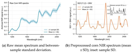
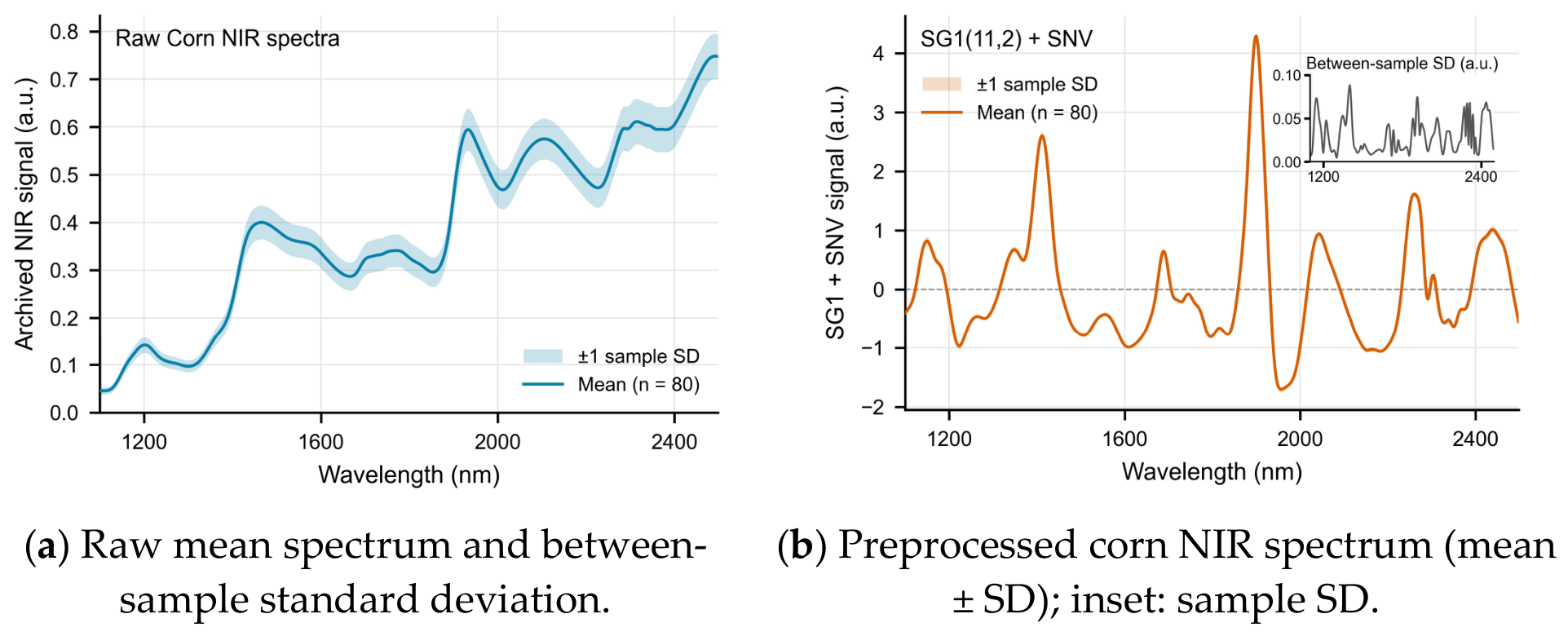
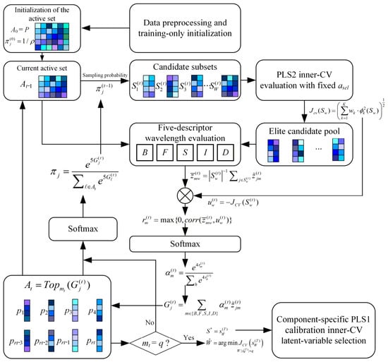
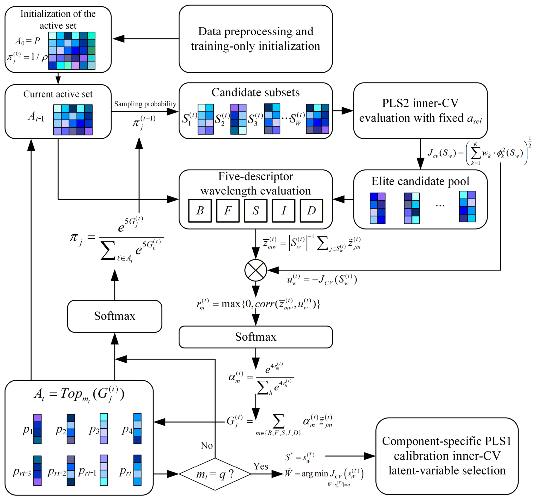
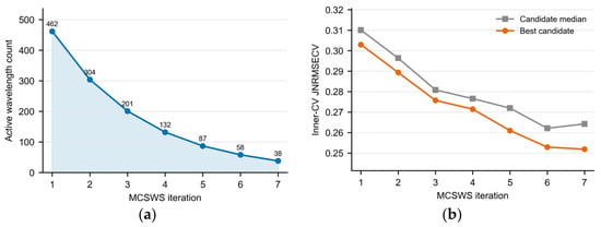
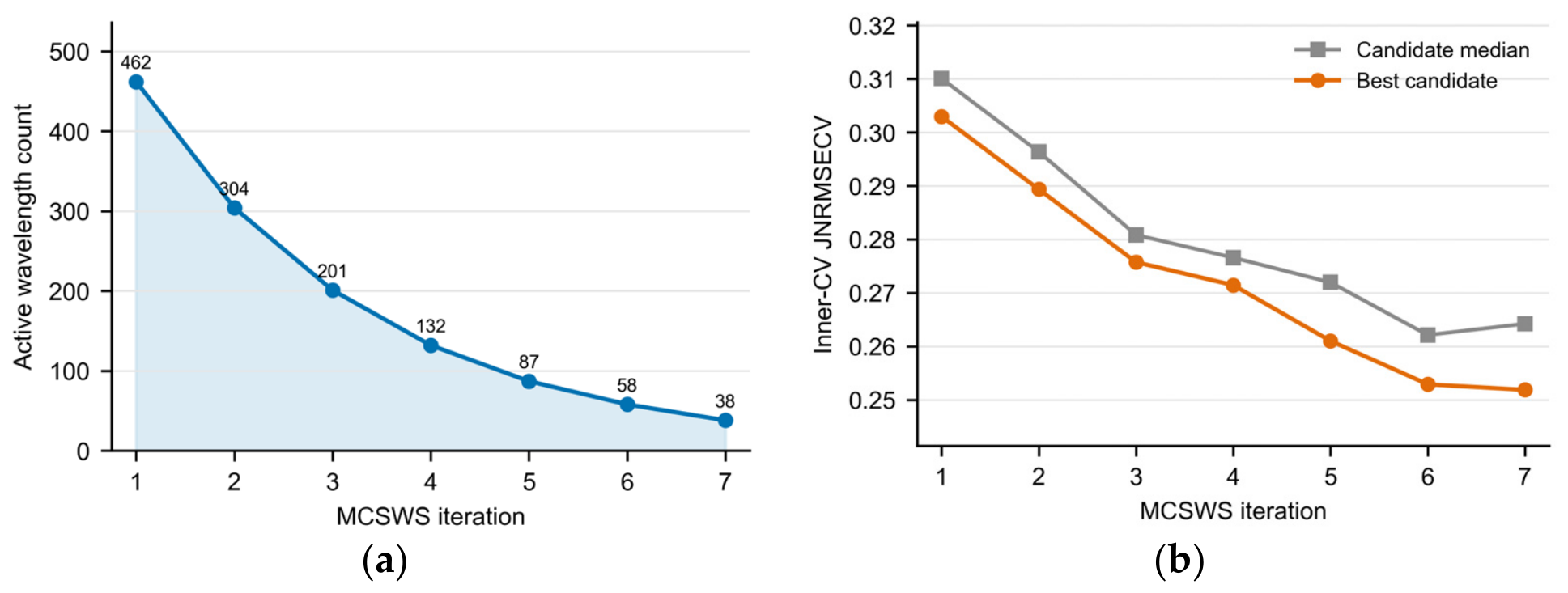
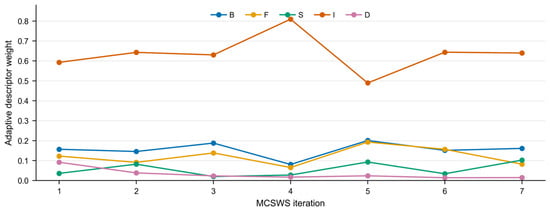
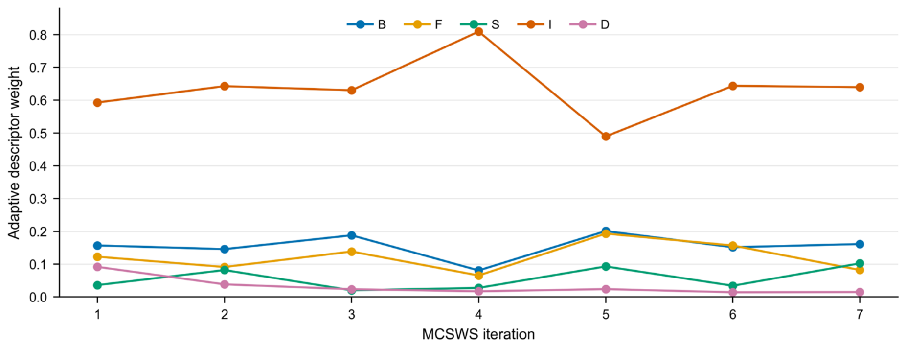
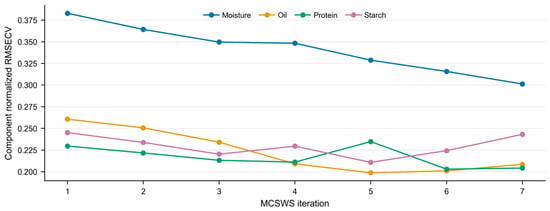
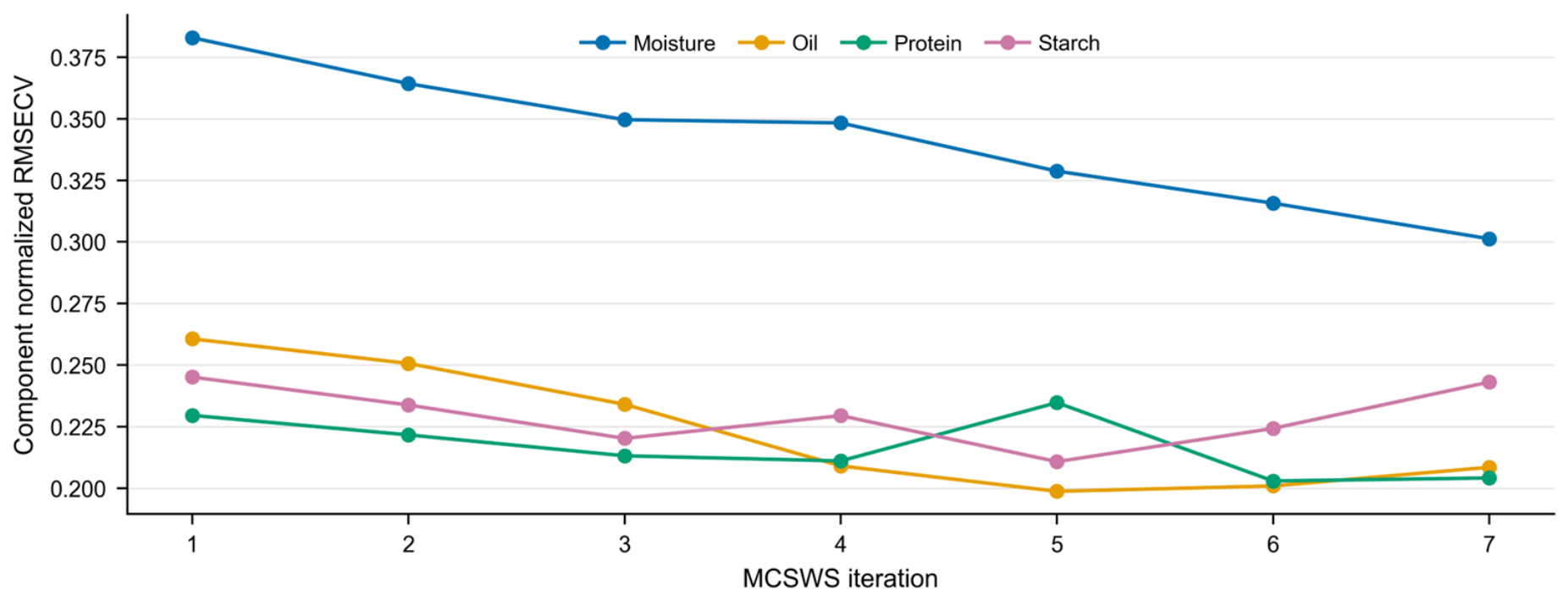
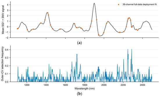
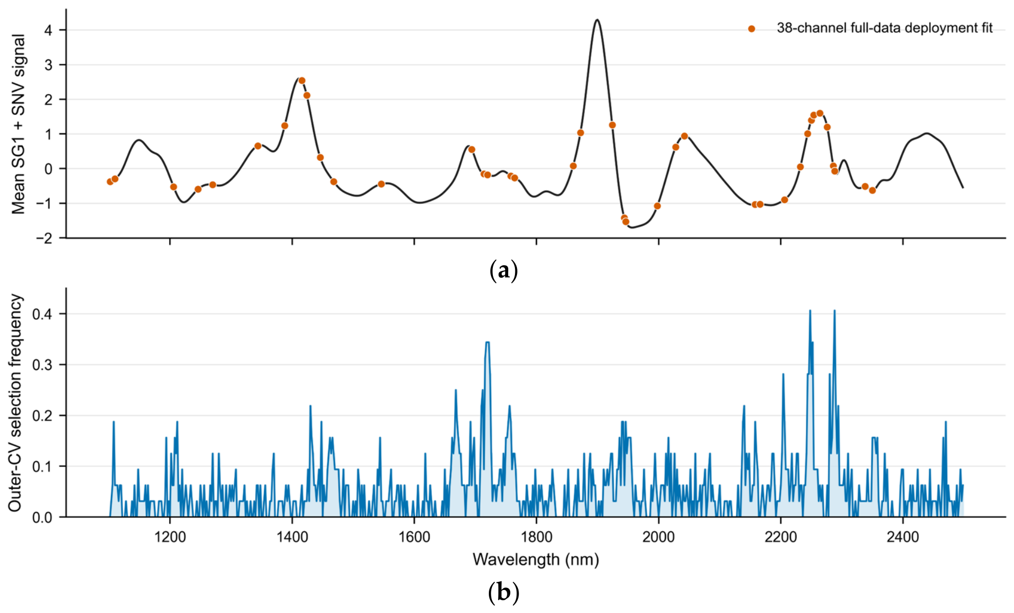
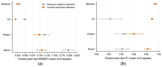
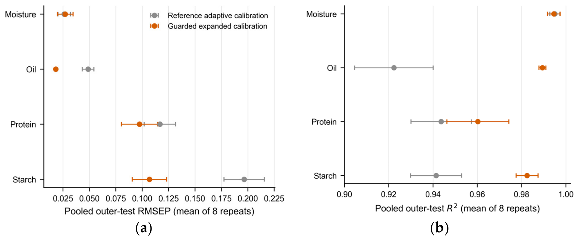
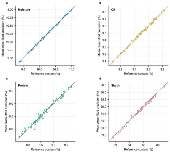
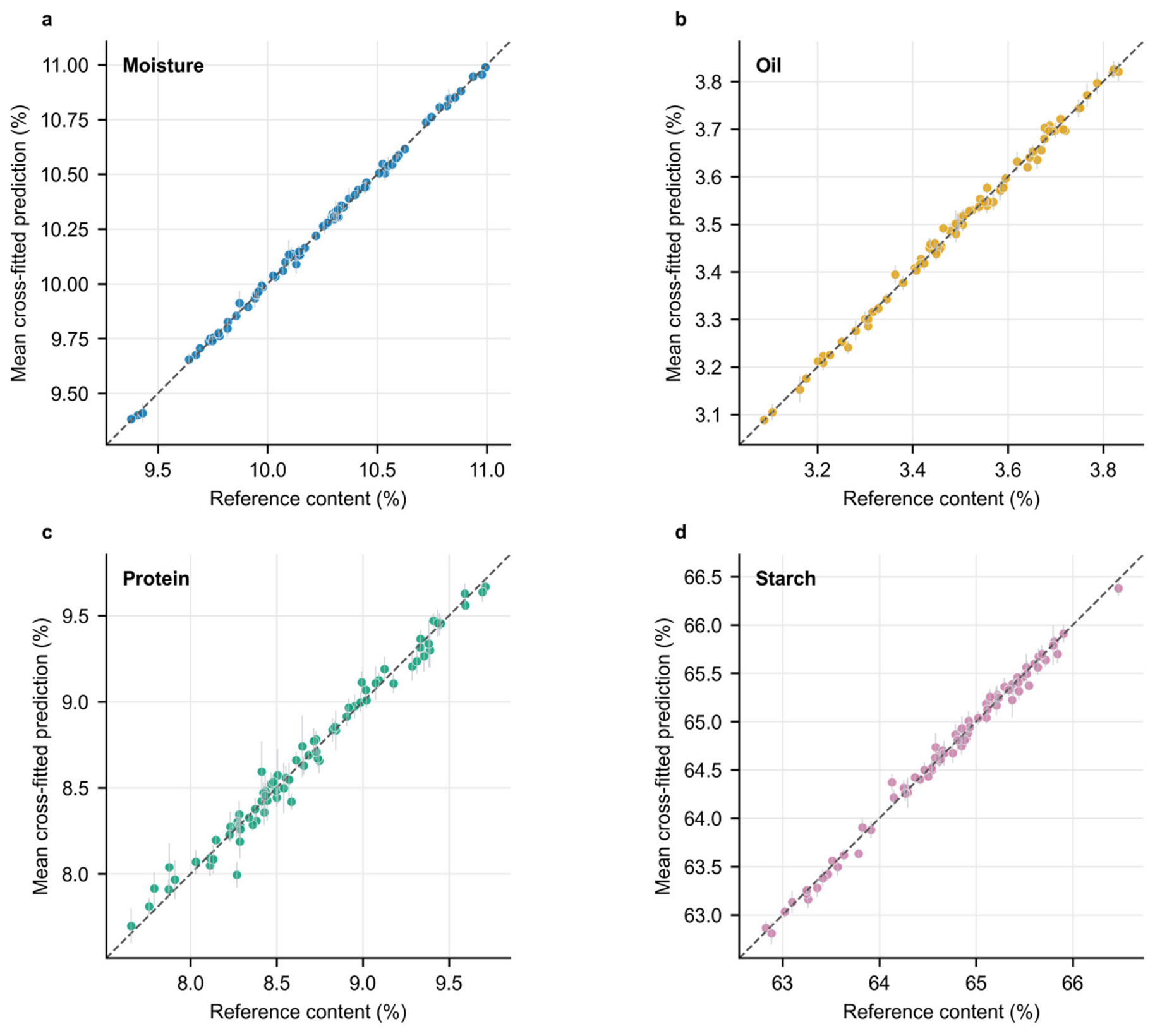
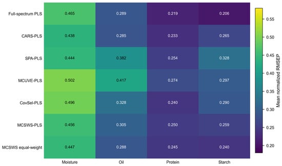
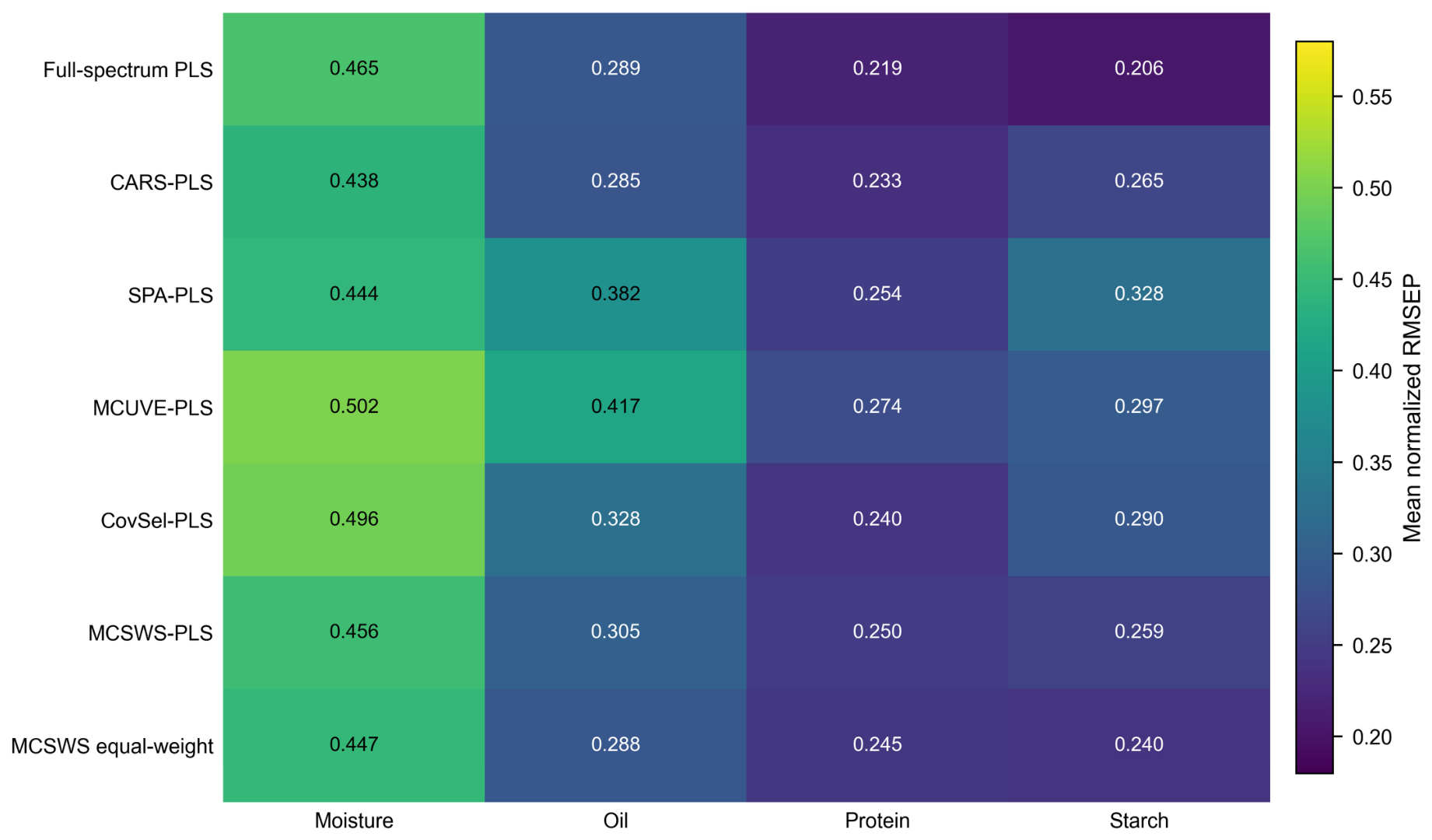
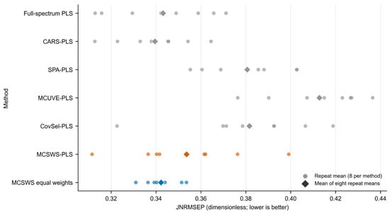
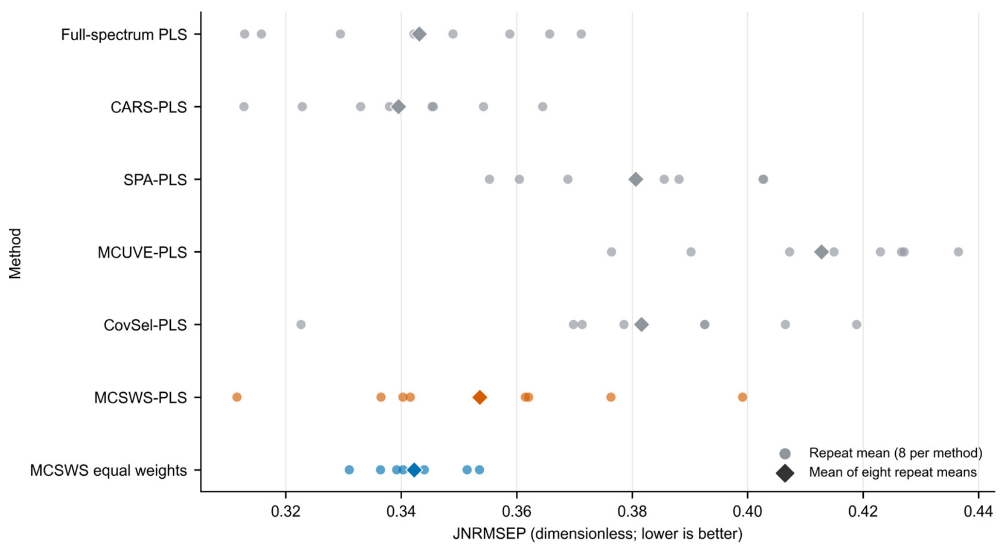
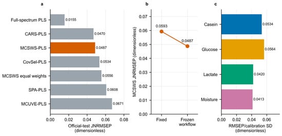
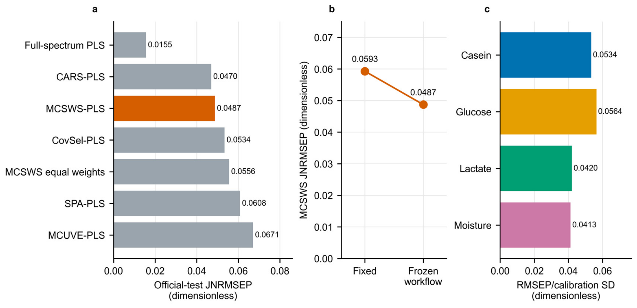

Disclaimer/Publisher’s Note: The statements, opinions and data contained in all publications are solely those of the individual author(s) and contributor(s) and not of MDPI and/or the editor(s). MDPI and/or the editor(s) disclaim responsibility for any injury to people or property resulting from any ideas, methods, instructions or products referred to in the content. |
© 2026 by the authors. Licensee MDPI, Basel, Switzerland. This article is an open access article distributed under the terms and conditions of the Creative Commons Attribution (CC BY) license.