A Texture-Aware CNN Predictor for Reversible Data Hiding

Abstract

Reversible data hiding (RDH) enables the reversible embedding of additional data into cover media, allowing the cover media to be perfectly recovered after extracting the embedded data. RDH relies on accurate prediction of pixels to generate sharply distributed prediction error histograms, thereby maximizing embedding capacity and minimizing visual distortion. While convolutional neural network (CNN)-based predictors excel in smooth regions of cover images by leveraging local correlation, they often fail to produce accurate predictions in the textured regions. To address the limitation of CNN predictors, we propose a novel attention fusion-based CNN predictor (AFCNNP) that adaptively combines the CNN predictor with a non-local means (NLM) predictor. The proposed fusion framework learns spatial weight maps to favor CNN predictions in smooth regions and NLM predictions in textured regions. The experimental results show that the proposed framework outperforms other state-of-the-art CNN predictors by significantly lowering the mean absolute error, mean squared error, and variance of prediction errors, leading to more accurate pixel predictions. With the proposed fusion framework, the embedding and visual performance of prediction error expansion (PEE)-based RDH is improved compared to typical CNN-based RDH methods.

1. Introduction

With the rapid development of information technologies and transmission systems, a huge amount of multimedia data is being outsourced and shared among end users. For privacy protection and data management, certain additional data, such as metadata, authentication data, notation information, and file category data, need to be transmitted along with the original content. Reversible data hiding is a branch of information hiding technologies that can reversibly embed additional data into multimedia [1,2,3]. Reversible embedding means that the original multimedia content can be losslessly reconstructed after extracting the additional data at the receiver side. This property of lossless media recovery is crucial to various sensitive applications such as military, medical, satellite imagery, and law forensics, where permanent distortion of the media due to embedding is unacceptable. Besides, RDH has been specifically used in integrity authentication [4,5,6], cover-lossless recovery [7], privacy protection [8], digital copyright protection [9], and medical imaging [10,11,12].

RDH has evolved over more than a decade, and numerous RDH methods have been proposed, characterized by low embedding capacities and high visual distortion, to methods with maximum embedding capacities reaching the upper capacity bound and with high-fidelity marked media [13,14]. The fundamental RDH methods can be classified into: (1) lossless compression (LC) [15], (2) difference expansion (DE) [16], and (3) histogram shifting (HS) [17]. In LC-based RDH, some features of the cover media are losslessly compressed to make room for additional data embedding. DE exploits redundancy in natural images by expanding the small differences of neighboring pixels for data embedding. The HS RDH method shifts the unevenly distributed histogram of natural images to reserve room for data embedding. Following DE and HS, prediction error expansion (PEE) has attracted considerable attention from the research community because of its ability to better exploit redundancy in natural images and maintain a trade-off between embedding capacity and marked image quality. The core principle of PEE is to generate a concentrated, high-amplitude prediction error histogram with minimum entropy and modify this histogram for data embedding [18,19].

In the literature, numerous predictors have been proposed to generate a sharply distributed prediction error histogram for PEE and improve prediction accuracy. These predictors estimate a central pixel by its local neighborhood pixels, which is also called the prediction context. These conventional predictors include: (1) difference predictor (DP) [16], (2) median edge detection predictor (MEDP) [20], (3) bilinear interpolation predictor (BIP) [21], (4) gradient adjusted predictor (GAP) [22], (5) partial differential equation predictor (PDEP) [23], (6) least square predictor (LSP) [24], and (7) multi-predictor (MP) [25]. While conventional predictors have achieved improved prediction accuracy, they rely on local prediction context and linear methods employing a limited number of neighboring pixels, restricting their accuracy, especially in complex images. While these predictors have improved prediction accuracy to some extent, their inability to fully exploit pixel correlations leaves room for improvement. A more effective approach would involve global, nonlinear prediction techniques that leverage a broader pixel context, enhancing prediction precision and overall performance.

The swift progress of deep learning has empowered CNN to demonstrate superior performance in diverse domains [26,27]. Leveraging their multi-receptive fields and global optimization capabilities, CNNs can serve as powerful predictors to enhance prediction accuracy in reversible data hiding (RDH). Hu et al. [28] presented the first CNN predictor (CCNP) for PEE-based RDH that divides a cover image into dot and cross set images. A lightweight CNN model is trained using one set of images to predict the other set of images using $N_{4}P$ neighboring pixels in the $3\times 3$ prediction context. CNNP significantly improved prediction accuracy compared to conventional predictors. Hu et al. [29] enhanced the prediction accuracy of CCNP through an advanced image division strategy where the cover image is divided into four distinct sets and one set is predicted by the other three sets of images. This improved CNNP expands the $3\times 3$ prediction context to incorporate six neighboring pixels. Additionally, prediction error ordering (PEO) is used to further enhance embedding performance in conjunction with the improved prediction method. In [30], Yang et al. proposed another CNN predictor and embedding method that divides a cover image into four sets and predicts one set using the other three sets. The key difference between the Hu et al. [29] improved method and the Yang et al. [30] is the image division strategy. Hu et al.’s improved method predicts the central pixel using its six neighbors in a $3\times 3$ neighborhood but utilizes 18 pixels in the $5\times 5$ prediction context, while the Yang et al. method utilizes eight pixels in the prediction context in a $3\times 3$ window and sixteen pixels in a $5\times 5$ window. Wu et al. [31] introduced a new image division strategy for improving the prediction accuracy of the CNN predictor. The cover image is separated into four independent sub-images. The proposed predictor uses 18 pixels in the $5\times 5$ neighborhood and full use of the eight pixels in the $3\times 3$ neighborhood for estimating the center pixel. In addition, shortcut connections and an attention mechanism are introduced in the CNN network to improve prediction accuracy. In [32], Lin et al. introduced a smoothing factor for the loss function of the CNNP framework that prioritizes smooth regions of the image by giving larger weights to smooth regions than textured regions. This solution significantly improved the prediction accuracy and embedding performance. Recently, Qiu et al. presented a CNN predictor similar to the Hu et al. [28] predictor but with an additional complexity computation block in the CNN framework [33]. This method achieved superior prediction performance compared to [28] due to predicting the complexity of each pixel. Zhao et al. presented a hybrid predictor for smooth and complex regions of image [34]. To predict smooth regions, a classical predictor is used, while more complex regions are predicted by a CNN predictor. A recent prediction value ordering (PVO) and CNN-based RDH method converts the image to a one-dimensional array for improved overlapping and embedding capacity [35]. Moreover, a deep neural network is employed to adaptively select suitable predictors for each pixel, thereby improving prediction accuracy and embedding performance. A novel CNN predictor for predicting color images was recently presented in [36], in which an image division method is designed so that the improved CNN predictor can take advantage of more adjacent pixels in the current channel. Zhou et al. presented a transformer-based predictor that leverages self-attention mechanisms to capture long-range dependencies and improve prediction accuracy [37].

In summary, all the CNNPs mentioned so far achieved satisfactory results in prediction accuracy and embedding performance. These CNNPs have either used prediction error ordering (PEO) to prioritize prediction errors for data embedding in smooth regions or integrated a smoothing factor with the loss function of the network to prefer predicting smooth regions more accurately. However, these methods predominantly optimize for local correlations in homogeneous regions, leaving textured regions—where non-local self-similarities dominate—unaddressed. This creates a critical bottleneck: while smooth regions achieve near-zero prediction errors, textured regions exhibit substantially higher errors, limiting the overall embedding capacity of the RDH method. Table 1 lists the details of classical and most relevant CNN predictors with respect to their performance in smooth and textured regions.

Table 1. Details of classical and CNN predictors.

Predictor	Type	Smooth Regions	Textured Regions	Embedding Capacity
[16]	Classical	Moderate accuracy	Poor, large errors	Low
[20]	Classical	Good in flat/edges	Fair in textures	Moderate
[21]	Classical	Excellent in smooth	Poor in textures	Low
[22]	Classical	Good in gradients	Fair; unstable in noise	Moderate
[23]	Classical	Excellent via diffusion	Fair; over-smooths	Moderate
[24]	Classical	Learns smooth structure	Moderate in textures	High
[25]	Classical	Adaptive	Good, partly robust	High
[28]	CNN	Trained for smoothness	Avoids textured areas	Moderate
[29]	CNN	Robust in smooth zones	Avoids high-error pixels	Moderate
[30]	CNN	Wide receptive field	Embeds selectively	Moderate
[31]	CNN	Sharp low-error preds	Excludes textures	Low
[32]	CNN	Weighted for smoothness	Texture downweighted	Low–Moderate
[33]	CNN	Low complexity selection	Excludes textures	Moderate

To overcome this limitation, we propose a unified framework that combines the strengths of CNNP (for smooth regions) and non-local means (NLM) (for textured regions) via an attention-guided fusion mechanism. By achieving low prediction errors across all image regions, not just smooth ones, our approach maximizes usable prediction errors for embedding, thus increasing potential payload capacity while maintaining visual fidelity. This is particularly vital for applications requiring high-capacity reversible embedding in complex images (e.g., medical or satellite imagery), where texture handling is as crucial as smooth region preservation. The main contributions of this work are as follows:

• We propose the first RDH method that combines CNN-based local prediction with NLM-based global prediction, achieving lower MAE and MSE in textured regions compared to CNNP-only methods while preserving CNNP’s accuracy in smooth regions.
• A lightweight attention network (2 convolutional layers) is introduced to automatically weight CNNP and NLM predictions per-pixel, eliminating manual thresholding that reduces prediction-error variance.
• By minimizing errors across both smooth and textured regions, our method increases usable prediction errors for embedding, enabling higher payload capacity at the same PSNR compared to state-of-the-art CNN predictors.

The rest of the paper is organized as follows. Section 2 presents the proposed method, including the fundamentals of prediction error expansion, the non-local means predictor, and the attention-based fusion of CNN and non-local predictors, followed by the proposed RDH method. Section 3 reports experimental results, including prediction accuracy and embedding performance. Finally, Section 4 concludes the paper.

2. Proposed Method

2.1. Prediction Error Expansion

PEE is a widely adopted embedding method in RDH due to its ability to embed additional data into images with low distortion. The essence of PEE is exploiting local redundancy in natural images by predicting pixels in a local neighborhood and embedding data by expanding the corresponding prediction errors. The objective is to obtain a sharply peaked prediction error histogram centered around zero, thereby embedding more data with minimal distortion. Let $p_{i,j}$ be a pixel value in a local neighborhood ${\mathcal{N}}_{i,j}$ in a grayscale image, its predicted value ${\widehat{p}}_{i,j}$ is computed using a prediction function $\mathcal{P}$ that estimates the pixel value based on its prediction context.

$${\widehat{p}}_{i,j}=\mathcal{P}\left(p_{i^{\prime },j^{\prime }}\right),(i^{\prime },j^{\prime })\in {\mathcal{N}}_{i,j}$$

(1)

The prediction error is defined as $e_{i,j}=p_{i,j}-{\widehat{p}}_{i,j}$. The prediction errors can be classified into inner, where $e_{i,j}\in [T_l,T_r)$, and outer where $e_{i,j}\in (-\infty ,T_l)\cup [T_r,+\infty )$ where $T_l/T_r$ are the two thresholds to control the trade-off between embedding capacity and distortion of the marked image. The inner prediction errors are expanded to embed one bit $b\in \{0,1\}$ of data as $e_{i,j}^w=2e_{i,j}+b$, and the outer prediction errors are shifted outward $T_l/T_r$ to create vacancy bins in the prediction error histogram and to guarantee reversibility. The marked pixel value is computed as given in Equation (2).

$$p_{i,j}^w=\left\{\begin{array}{cc}{p}_{i,j}+e_{i,j}+b,\hfill & \mathrm{if}{e}_{i,j}\in [T_l,T_r)\hfill \\ p_{i,j}+T_r,\hfill & \mathrm{if}{e}_{i,j}\in [T_r,+\infty )\hfill \\ p_{i,j}+T_l,\hfill & \mathrm{if}{e}_{i,j}\in (-\infty ,T_l)\hfill \end{array}\right.$$

(2)

After data embedding, the expanded prediction error of inner pixels is shifted to $e_{i,j}^w\in [2T_l,2T_r)$ and outer pixels are shifted to $e_{i,j}^w\in (-\infty ,2T_l)\cup [2T_r,+\infty )$. To maintain reversibility, pixels for which the marked error $e_{i,j}^w$ would cause the underflow/overflow issue, i.e., $p_{i,j}^w\notin [0,255]$, are excluded or recorded using a location map.

At the receiver side, given the marked image and the same prediction function $\mathcal{P}$, the expanded prediction error is computed using Equation (3):

$$e_{i,j}^w=p_{i,j}^w-{\widehat{p}}_{i,j}$$

(3)

After generating the expanded prediction error histogram and given $T_l/T_r$, the original prediction error is recovered using Equation (4):

$$e_{i,j}=\left\{\begin{array}{cc}⌊{\displaystyle \frac{e_{i,j}^w}{2}}⌋,\hfill & \mathrm{if}{e}_{i,j}^w\in [2T_l,2T_r)\hfill \\ e_{i,j}^w-T_r,\hfill & \mathrm{if}{e}_{i,j}^w\in [2T_r,\infty )\hfill \\ e_{i,j}^w-T_l,\hfill & \mathrm{if}{e}_{i,j}^w\in (-\infty ,2T_l)\hfill \end{array}\right.$$

(4)

The embedded bits are extracted by $b=e_{i,j}^w\mathrm{mod}2$ and the original pixel value is restored as $p_{i,j}={\widehat{p}}_{i,j}+e_{i,j}$. In this way, all the embedded data are extracted, and the original image is restored.

2.2. Non-Local Means

Non-local means is a powerful image denoising and prediction method that is used to exploit the self-similarity property in natural images. As described in Section 2.1, conventional PEE predictors rely solely on local prediction context for pixel prediction. In contrast, NLM finds non-local repeated patterns across the entire image to obtain accurate predictions even in highly textured and complex images. Instead of predicting a pixel by its local prediction context, NLM averages the values of all pixels throughout the images that share similar surrounding patches.

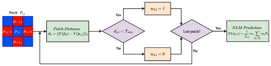
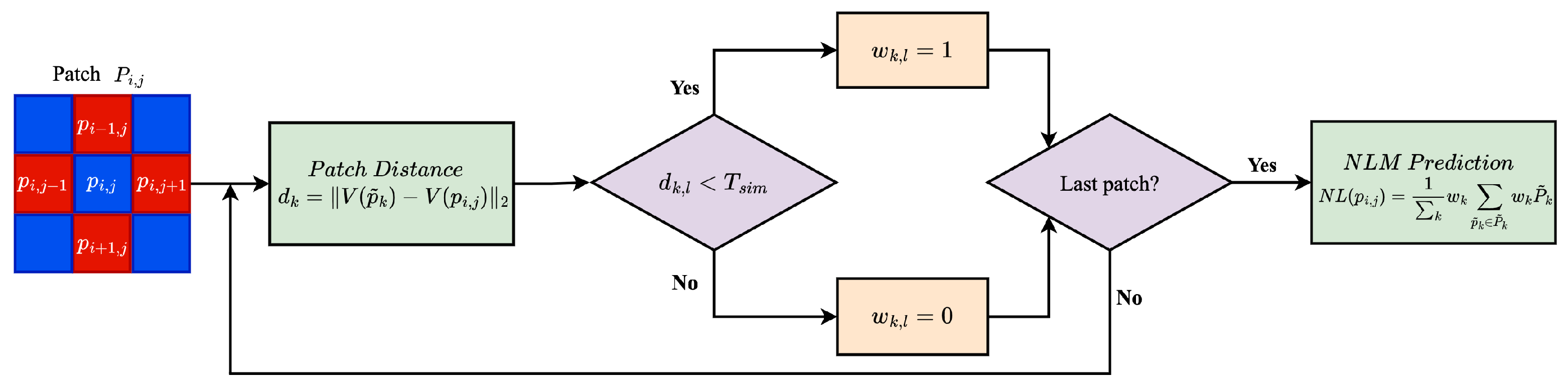
We present a modified version of the original NLM that is suitable for integration with CNNP. The flow diagram of the modified NLM prediction is illustrated in Figure 1.

Figure 1. The flow diagram of NLM prediction.

Let $P_{i,j}$ be a rhombus pattern patch centered at pixel $p_{i,j}$ with its four nearest neighbors $p_{i+1,j}$, $p_{i-1,j}$, $p_{i,j+1}$, and $p_{i,j-1}$, and let ${\mathcal{N}}_p$ of size $w\times w$ be a large search window. The NLM prediction of pixel $p_{i,j}$$NL\left(p_{i,j}\right)$ is given by Equation (5):

$$NL\left(p_{i,j}\right)={\displaystyle \frac{1}{{\sum }_k{w}_k}}\sum _{{\tilde{p}}_k\in {\tilde{P}}_k}{w}_k{\tilde{p}}_k$$

(5)

where ${\tilde{p}}_k$ is a non-local pixel and $w_k$ is the weight determined by the similarity between the local patch $P_{i,j}$ and the non-local patch ${\tilde{P}}_k$. The similarity between two patches is computed by the Euclidean distance as given in Equation (6).

$$d_k={∥V\left({\tilde{p}}_k\right)-V\left(p_{i,j}\right)∥}_2$$

(6)

To determine whether two patches are similar enough to be considered in the prediction of a pixel, a user-defined threshold $T_{sim}$ is used to consider only similar patches and disregard dissimilar ones. Equation (7) is used to adaptively assign the associated weight.

$$w_k=\left\{\begin{array}{c}1,d_k\le T_{\mathrm{sim}}\hfill \\ 0,\mathrm{Otherwise}\hfill \end{array}\right.$$

(7)

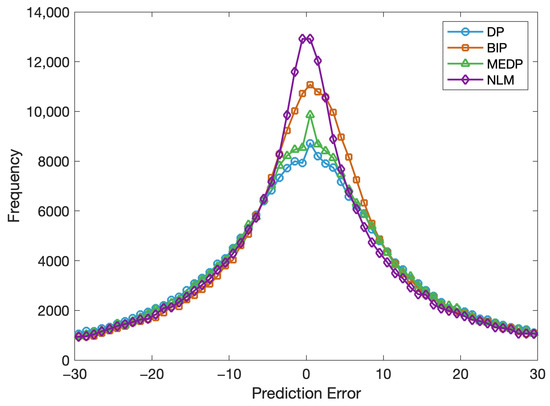
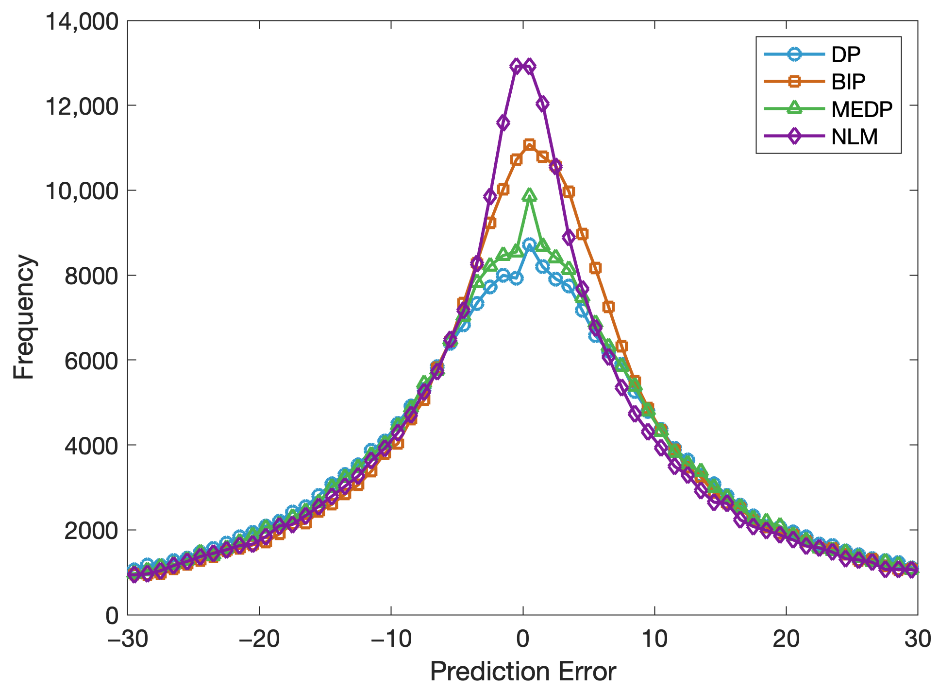
As described earlier, NLM is specifically effective in predicting pixels in textured regions. To prove the effectiveness of NLM in the Baboon textured image, prediction error histograms of NLM and three conventional predictors are plotted as shown in Figure 2. It can be noted that the prediction error histogram of NLM is higher and sharper than the histograms of the other three predictors.

Figure 2. Prediction error histograms of NLM and three conventional predictors for the Baboon image.

The distribution of prediction error histogram is defined by the entropy as computed in Equation (8)

$$E=-\sum _{e}p\left(e\right)ln\left(p\left(e\right)\right),$$

(8)

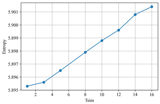
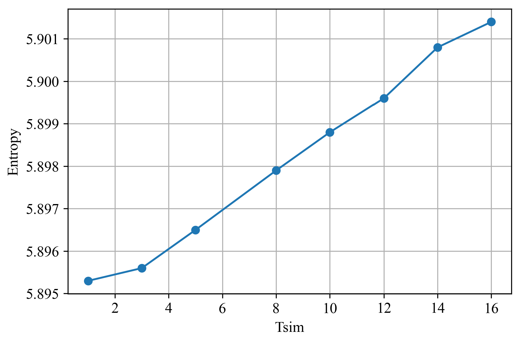
where $p(·)$ is the probability and e is the prediction error. To analyze the sensitivity of prediction error statistics with respect to $T_{sim}$, we plotted the entropy of prediction errors against increasing $T_{sim}$ values for the Baboon image as shown in Figure 3. A smaller value of $T_{sim}$ selects highly similar patches for prediction and hence results in low entropy of prediction error distribution. However, this limits the ability of the NLM to exploit non-local redundancy. Larger values of $T_{sim}$ include less similar patches, which ultimately increases the entropy of the prediction error distribution. This trend is observed in Figure 3 where the entropy increases monotonically with increasing values of $T_{sim}$. This highlights the importance of carefully selecting $T_{sim}$.

Figure 3. Entropy of prediction errors against increasing $T_{sim}$.

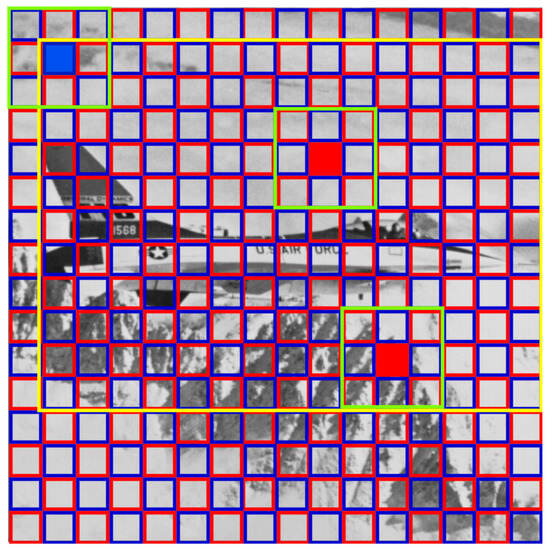
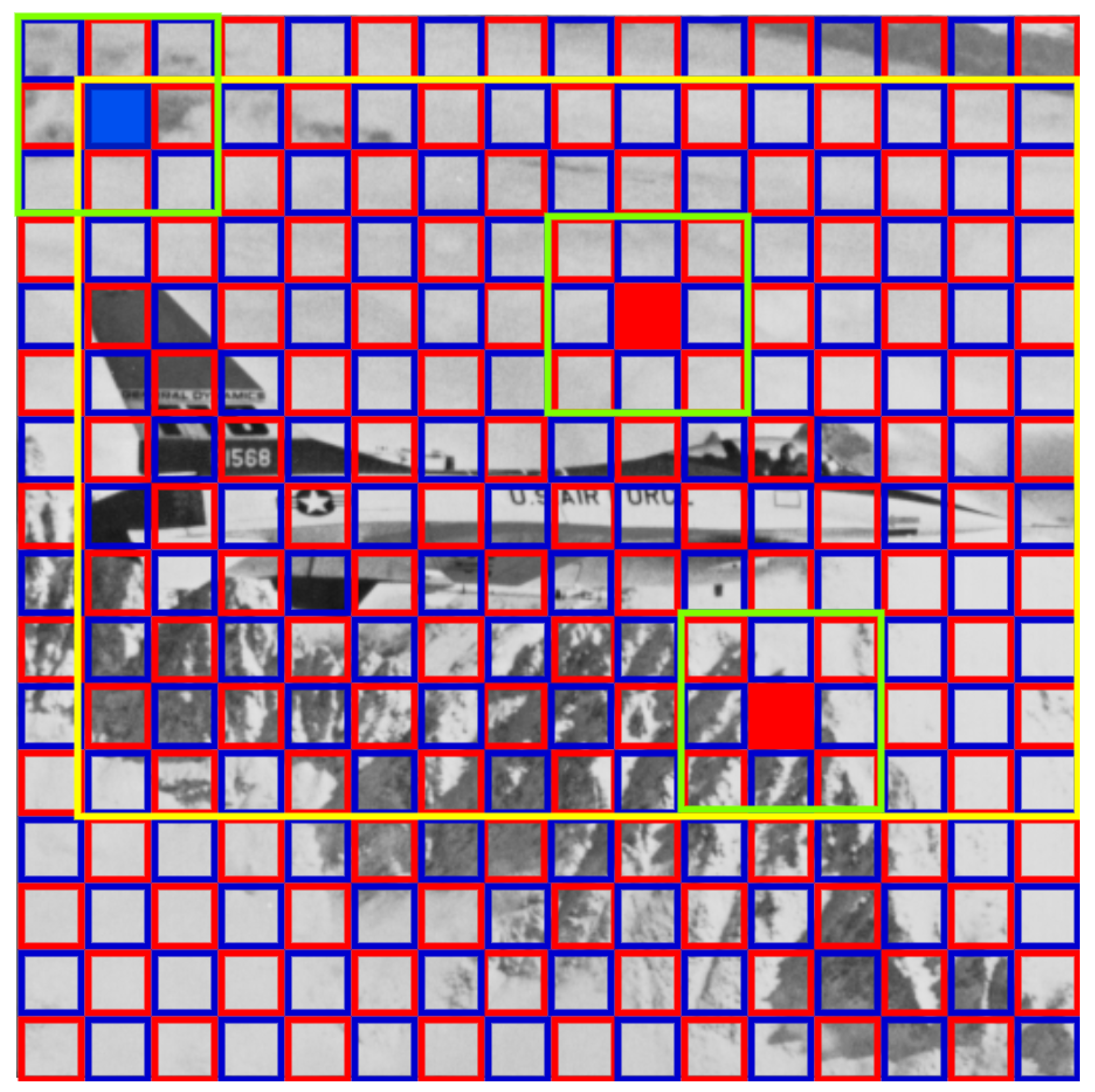
To seamlessly integrate with the CNNP framework and achieve reversibility in the RDH method, the image division strategy proposed in [28] is adopted for NLM. The original image $\mathbf{p}$ is partitioned into two independent sets $p_A=\{p_{i,j}\mathrm{mod}2=0\}$ and $p_B=\{p_{i,j}\mathrm{mod}2=1\}$ and one set is used to predict the other set and vice versa. Let the $p_A$ image be predicted by the $p_B$ image in the first round. The to-be-predicted pixels are scanned in raster scan order from left to right. It is worth noting that patch similarity is computed using the original image, but only the central pixels in the patch from $p_B$ pixels are averaged for prediction. This scenario is illustrated in Figure 4 where $p_A$ is marked by blue color and $p_B$ is marked by red color bounding boxes, representing dot and cross sets respectively. The goal is to predict the center pixel of a green patch located within the dot set (blue box), where prediction must rely exclusively on unmodified pixels from the opposite (cross) set. In the search window (highlighted in yellow), candidate patches from the cross-pixel set are extracted. Candidate patches satisfying the similarity threshold are selected for non-local prediction. In this example, two valid non-local patches with central pixels from the cross set are identified and highlighted with red color. These central pixels contribute only to the prediction of the current dot pixel (blue box). This setup guarantees that the prediction context remains invariant during embedding and extraction, thereby enabling perfect reversibility.

Figure 4. Image division strategy for NLM prediction.

2.3. Attention-Based Fusion of CNN and Non-Local Predictors

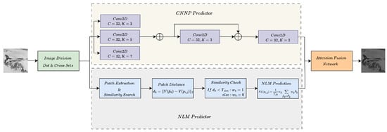
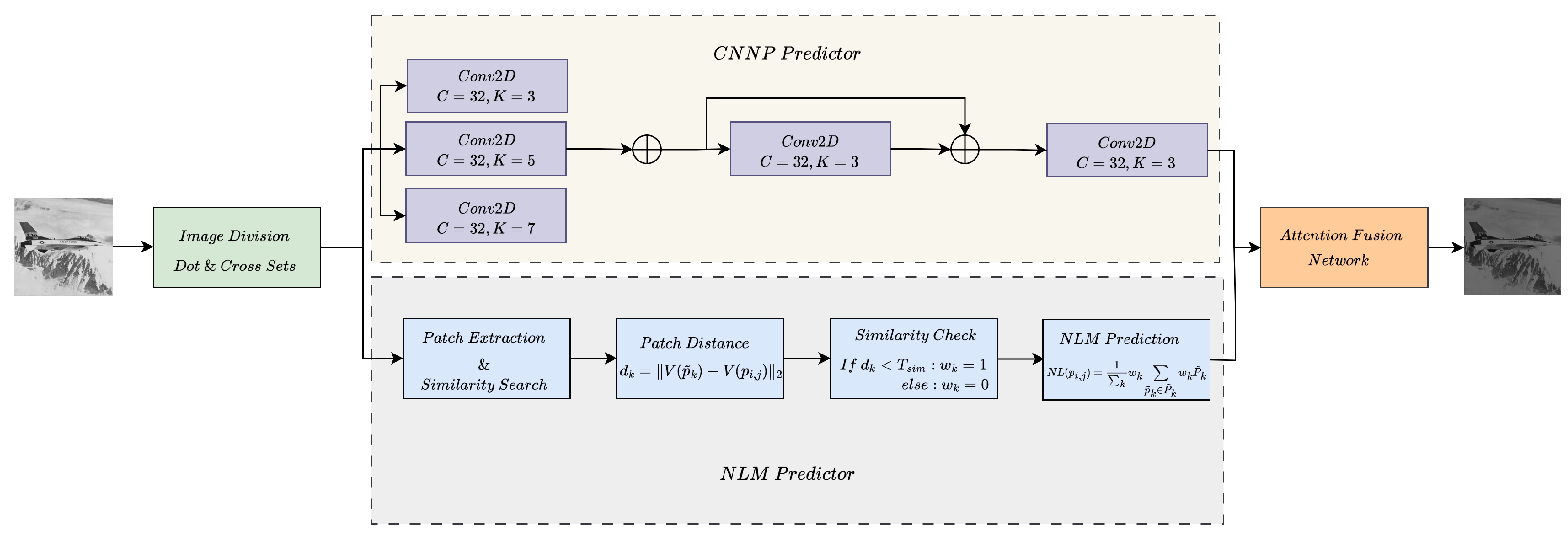
This section presents the proposed AFCNNP framework that combines the predictions of CNNP and the NLM predictor through an attention mechanism. We use the architecture of CNNP as presented in [28] for the CNN prediction. This proposed framework is illustrated in Figure 5, which consists of the CNNP predictor, NLM predictor, and attention fusion network. Let $I\in {\mathbb{R}}^{H\times W}$ be an input image. The CNNP prediction $P_{\mathrm{CNNP}}(i,j)$ at a pixel $(i,j)$ can be computed using Equation (9):

$$P_{\mathrm{CNNP}}(i,j)=f_{\theta }\left({\mathcal{V}}_k(I(i,j)\right)$$

(9)

where $f_{\theta }$ is a pre-trained CNN with fixed weights $\theta$, ${\mathcal{V}}_k(I(i,j)$ is a local patch of $k\times k$ centered at $(i,j)$.

Figure 5. Proposed unified framework of CNNP and NLM.

The original image is divided into dot and cross sets and simultaneously fed to CNNP and NLM predictors. The CNNP employs a lightweight CNN network with a receptive field to perform local predictions based on local correlation. The NLM generates non-local predictions using a $3\times 3$ patch and $21\times 21$ search window. The resultant predictions from both CNNP and NLM are fed into an attention network designed to learn adaptive fusion weights. The goal of the attention fusion network is to generate pixel-wise attention weights that adaptively balance the contributions of local CNNP and non-local NLM predictions. The architecture of the attention fusion network is illustrated in Figure 6, which consists of two convolutional layers, a ReLU, and a Sigmoid activation function. The first CNN layer is a fully connected $3\times 3$ convolution with 16 filters and a padding of 1, followed by a ReLU activation function. The second layer is another $3\times 3$ convolution used to produce a single-channel attention weight.

Figure 6. Architecture of the attention fusion network.

Let $P_{CNNP}$ and $P_{NLM}$ be the prediction maps from CNNP and NLM with shape $(B,1,H,W)$, where B is the batch size of single-channel maps. These two prediction maps are concatenated along the channel dimension to form a tensor of shape $(B,2,H,W)$. The attention fusion network blends together the concatenated prediction maps using pixel-wise attention weights $\alpha (i,j)\in [0,1]$. The attention weights are computed using Equation (10).

$$\alpha (i,j)=\sigma \left({\mathbf{W}}_2·ReLU\left({\mathbf{W}}_1·\left[P_{\mathrm{CNNP}}(i,j);P_{\mathrm{NLM}}(i,j)\right]+{\mathbf{b}}_1\right)+{\mathbf{b}}_2\right)$$

(10)

where $[P_{CNNP};P_{NLM}]\in {\mathbb{R}}^2$ are the concatenated predictions, ${\mathbf{W}}_1\in {\mathbb{R}}^{16\times 2},{\mathbf{b}}_1\in {\mathbb{R}}^{16}$ are the first-layer weights and biases, ${\mathbf{W}}_2\in {\mathbb{R}}^{1\times 16},{\mathbf{b}}_2\in {\mathbb{R}}^1$ are the second layer weights and biases, and $\sigma$ is the Sigmoid function. The final fused prediction is computed using Equation (11):

$$P_{\mathrm{fused}}(i,j)=\alpha (i,j)P_{\mathrm{CNNP}}(i,j)+(1-\alpha (i,j))P_{\mathrm{NLM}}(i,j)$$

(11)

In Equation (11), the attention weight $\alpha (i,j)$ adaptively balances the contribution of CNNP and NLM predictors. The attention network prioritizes CNNP for $\alpha \to 1$ in smooth regions and NLM for $\alpha \to 0$ in textured regions.

In existing works [28,29,30,31,32], pixels in smooth regions are selected to generate sharp prediction error histograms, and pixels in textured regions are either not selected or downweighted in their loss functions, thereby limiting the total embedding capacity. This common approach of selecting only smooth regions of cover images overlooks the potential non-local self-similarity that exists even in textured regions of natural images, where NLM can generate reliable predictions. To address this limitation, we introduce a novel loss function to train the attention fusion network, which is given in Equation (12).

$$\mathcal{L}={\displaystyle \frac{1}{HW}}\sum _{i,j}\mid I(i,j)-P_{\mathrm{fused}}(i,j)\mid +\psi ·\mathrm{Var}(I-P_{\mathrm{fused}})$$

(12)

where $\psi$ is the regularization parameter and is set to 0.3. In Equation (12), the first term is the mean absolute error (MAE) between the ground truth pixels and the final fused predictions. The second term is the variance regularization. The first term tries to make predictions as close as possible to the true pixel values, while the second term forces the prediction errors to follow a desired distribution. With MAE and variance regularization in the loss function $\mathcal{L}$, the attention fusion network is trained to optimize prediction accuracy not only in smooth regions but also in textured regions where NLM proves beneficial. This formulation broadens the scope of usable pixels for embedding, resulting in higher embedding capacity with minimum distortion.

2.4. Proposed RDH Method

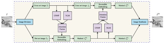
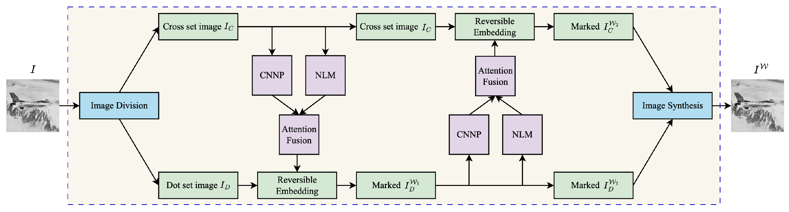
In this section, we present the proposed hybrid predictor-based RDH method that is illustrated in Figure 7. The original image is first divided into Dot ($I_D$) and Cross ($I_C$) sub-images. In the first phase of embedding, $I_C$ is used to generate the predicted Dot image ${\tilde{I}}_D$. Subsequently, $I_D$ and ${\tilde{I}}_D$ are used to generate, expand, and shift the prediction error histogram to embed a part of additional data ${\mathcal{W}}_1$. In this way, the marked Dot image $I_D^{{\mathcal{W}}_1}$ is generated. In the second phase of embedding, $I_D^{{\mathcal{W}}_1}$ is fed to the hybrid predictor to generate the predicted Cross image ${\tilde{I}}_C$, which is used to embed the second part of the additional data ${\mathcal{W}}_2$ to produce the marked Cross image $I_C^{{\mathcal{W}}_2}$. The marked Dot ($I_D^{{\mathcal{W}}_1}$) and Cross ($I_C^{{\mathcal{W}}_2}$) images are combined to generate the final marked image $I^{\mathcal{W}}$.

Figure 7. The proposed embedding method.

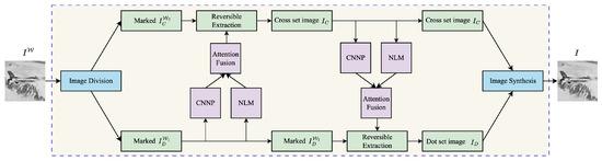
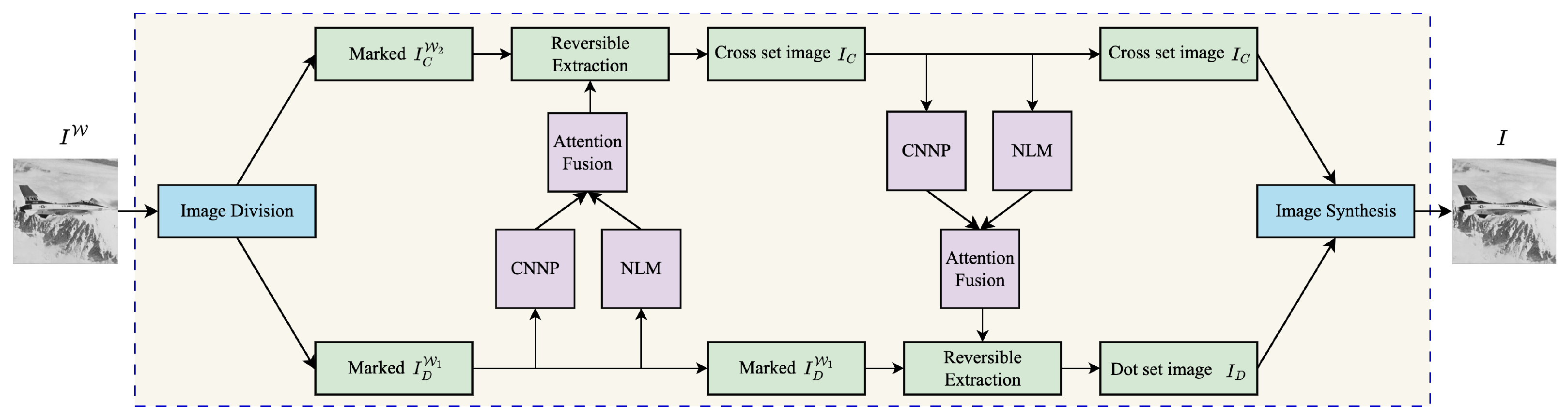
The data extraction and image recovery process is shown in Figure 8. The marked image $I^{\mathcal{W}}$ is divided into the marked Dot and Cross set images ($I_D^{{\mathcal{W}}_1}$, $I_C^{{\mathcal{W}}_2}$) using the same division strategy. The extraction process is the reverse of the embedding process, as the Cross set image $I_C$ is restored before the Dot set image $I_D$. The marked Dot image ($I_D^{{\mathcal{W}}_1}$) is fed to the trained hybrid predictor to predict the Cross set image ${\tilde{I}}_C$ which is used with the marked Cross set image ($I_C^{{\mathcal{W}}_2}$) to extract ${\mathcal{W}}_2$ and restore the original Cross set image $I_C$. After this, the restored Cross set image $I_C$ is used to predict the Dot set image ${\tilde{I}}_D$, which is then used to extract ${\mathcal{W}}_1$ and restore the original Dot set image $I_D$. Finally, the Dot set image $I_D$ and Cross set image $I_C$ are combined to restore the original image, and the data bits ${\mathcal{W}}_1$ and ${\mathcal{W}}_2$ are concatenated to obtain the additional data bits $\mathcal{W}$.

Figure 8. The proposed extraction method.

3. Experimental Results

In this section, we present extensive experiments to evaluate the performance of the proposed hybrid prediction method. The performance of the proposed method is compared with several advanced CNN predictors. It is worth mentioning that the transformer-based predictor by Zhou et al. [37] leveraged self-attention mechanisms to capture global contextual information. However, this predictor requires large-scale end-to-end training and does not explicitly distinguish between smooth and textured regions. Due to these fundamental differences in design and scope between the proposed predictor and the transformer-based predictor, a direct qualitative comparison is not considered in this work. We consider mean absolute error (MAE), mean squared error (MSE), and variance to compare prediction accuracy, and peak signal-to-noise ratio (PSNR) to compare embedding performance. The proposed AFCNNP is trained using 3000 images randomly selected from the ImageNet dataset [38]. These images are converted to grayscale with a size of $512\times 512$. Following established practices in CNN-based predictors [28,29,30,31,32,33], the model is trained using the Adam optimizer [39] with an initial learning rate of $1\times {10}^{-4}$, weight decay of $1\times {10}^{-3}$, and a batch size of 8. The Adam hyperparameters are set to default values (${\beta }_1=0.9$, ${\beta }_2=0.999$, $ϵ=1\times {10}^{-8}$). The network is trained for 20 epochs using standard backpropagation [40]. For experimental analysis and comparison purposes, we consider 6 benchmark grayscale images of size $512\times 512$ from the ucid.v2 dataset [41]. These images are Lena, Baboon, Boat, Barbara, Pepper, and Lake. The proposed method is implemented in Python 3.11.2 using PyTorch 2.6.0, and experiments were conducted on a Windows-based server equipped with an Intel(R) Core(TM) i9-10980XE CPU @ 3.00 GHz, 64 GB RAM, and an NVIDIA RTX A5000 GPU.

3.1. Prediction Accuracy

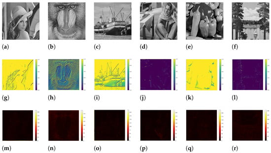
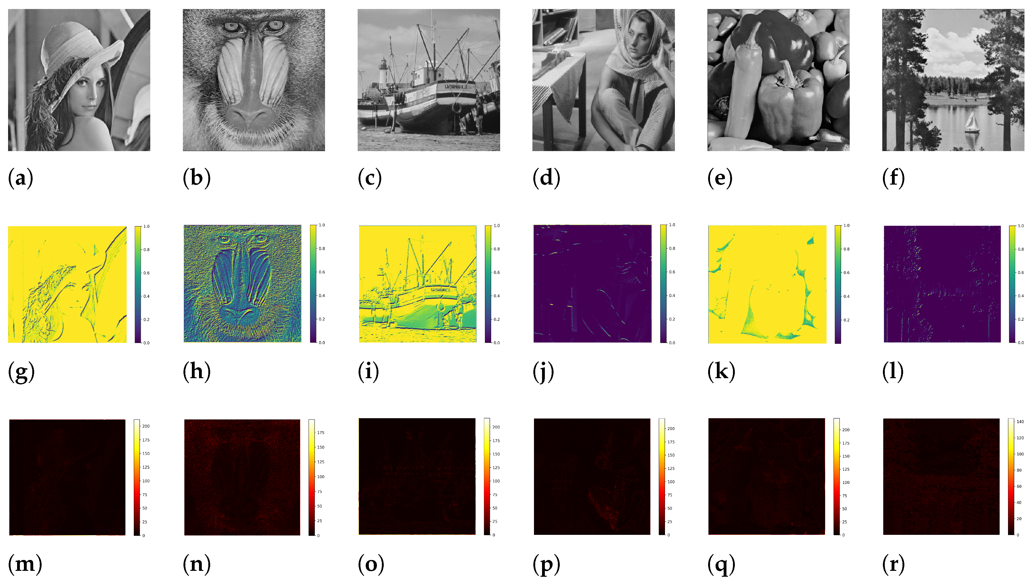
To demonstrate the effectiveness of the proposed AFCNNP, we present a comparative visualization of the fusion weight map for predicted regions in test images generated by CNNP and NLM as shown in Figure 9, where the original images are illustrated in the first row (a–f), and the fusion weight maps are depicted in the second row (g–l). For enhanced interpretability, we assign distinct colors to image regions based on the values of the attention weight $\alpha$. We assign yellow to CNNP-dominant regions ($\alpha >0.8$), indicating high confidence in localized feature extraction; blue to NLM-dominant regions ($\alpha <0.2$), highlighting reliance on non-local contextual information; and shades of yellow and blue (soft blending) to intermediate contributions ($0.2\le \alpha \le 0.8)$, where the network balances both models. The attention weight $\alpha$ dynamically governs the contribution of each predictor based on the localized features. In Figure 9g–l, CNNP dominates most of the regions of Lena, Boat, and Pepper, and NLM dominates in Barbara and Lake images. In the Baboon image, the fur texture is extremely dense, fine-grained, and varies rapidly in intensity and direction, resulting in small details changing sharply across neighboring pixels. Because of these sharp variations, the proposed AFCNNP softly blends the CNNP and NLM predictors, resulting in shades of yellow and blue colors in the weight map image. The $\alpha$-driven adaptive switching highlights the Attention Fusion network’s ability to combine CNNP’s local accuracy with NLM’s global coherence to achieve enhanced prediction accuracy.

Figure 9. Fusion weight and absolute error maps of predicted test images. (a–f): Original test images, (g–l): Fusion weight map images, (m–r): Absolute error map images.

The absolute error maps of test images are shown in Figure 9m–r. These error maps highlight the discrepancies between the fused predicted image and the original image. The error maps illustrate that the fused output achieves the lowest mean absolute error, particularly in textured regions where adaptive fusion is critical.

The proposed fusion predictor is compared with four CNN predictors [28,29,30,31,32] on 100 images from the ucid.v2 database [41]. Because integrating the smoothing factor of [32] into the predictor model of [31] offered superior embedding performance in terms of average PSNR on eight test images and the Kodak dataset, we consider only this integration in our comparative analysis. We compute average MAE, MSE, and variance between the original images and their corresponding predicted images for the proposed and other methods as listed in Table 2. As seen, the values of MAE, MSE, and variance computed using the proposed AFCNNP are lower than all the existing CNN predictors. As mentioned in Section 1, the Lin et al. predictor down-weighted prediction errors in textured regions and considered prediction errors of smooth regions only. This achieved accurate predictions in smooth regions but performed worse in textured regions, as claimed by the authors. In comparison, the proposed method achieves superior prediction and embedding performance not only in smooth regions but also in textured regions.

Table 2. Performance comparison of different predictors on prediction error statistics.

Predictor	Hu et al. [28]	Hu et al. [29]	Yang et al. [30]	Wu et al. [31]	Lin et al. [32]	Proposed
MSE	92.41	79.57	59.72	57.31	53.23	51.5
Mean	4.42	4.31	3.70	3.59	3.41	3.3
Variance	63.17	52.34	39.67	37.78	35.30	34.0

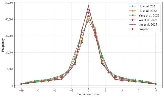
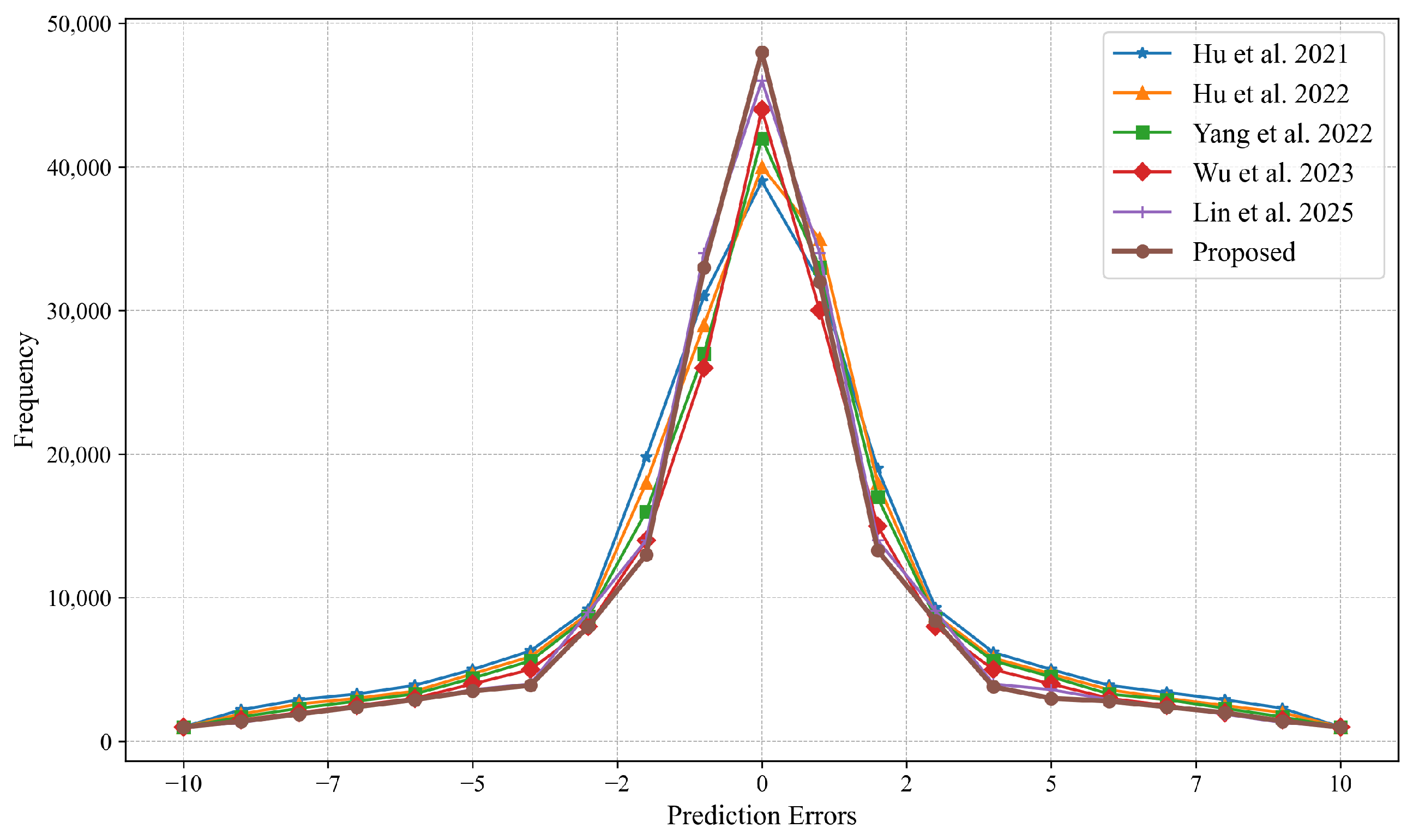
To visually demonstrate the superior prediction performance of the proposed method, we have plotted average prediction error histograms of five predictors on the ucid.v2 database as shown in Figure 10. The horizontal axis represents the prediction error values, and the vertical axis represents the frequency of prediction errors. For better display, the horizontal axis is set to [−10, 10]. It is worth noting that the prediction error histograms generated by the proposed AFCNNP are more concentrated around the zero value and have higher peaks than the histograms generated by other predictors. This is because the integration of NLM in the fusion network adds more accurate predictions, even from textured regions, to the pool of acceptable predictions, thus resulting in higher and sharper peaks in the prediction error histogram.

Figure 10. Comparison of average prediction error histogram of five predictors Hu et al. [28], Hu et al. [29], Yang et al. [30], Wu et al. [31] and Lin et al. [32] on ucid.v2 database.

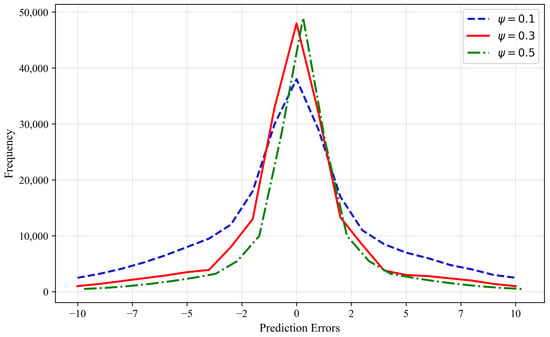
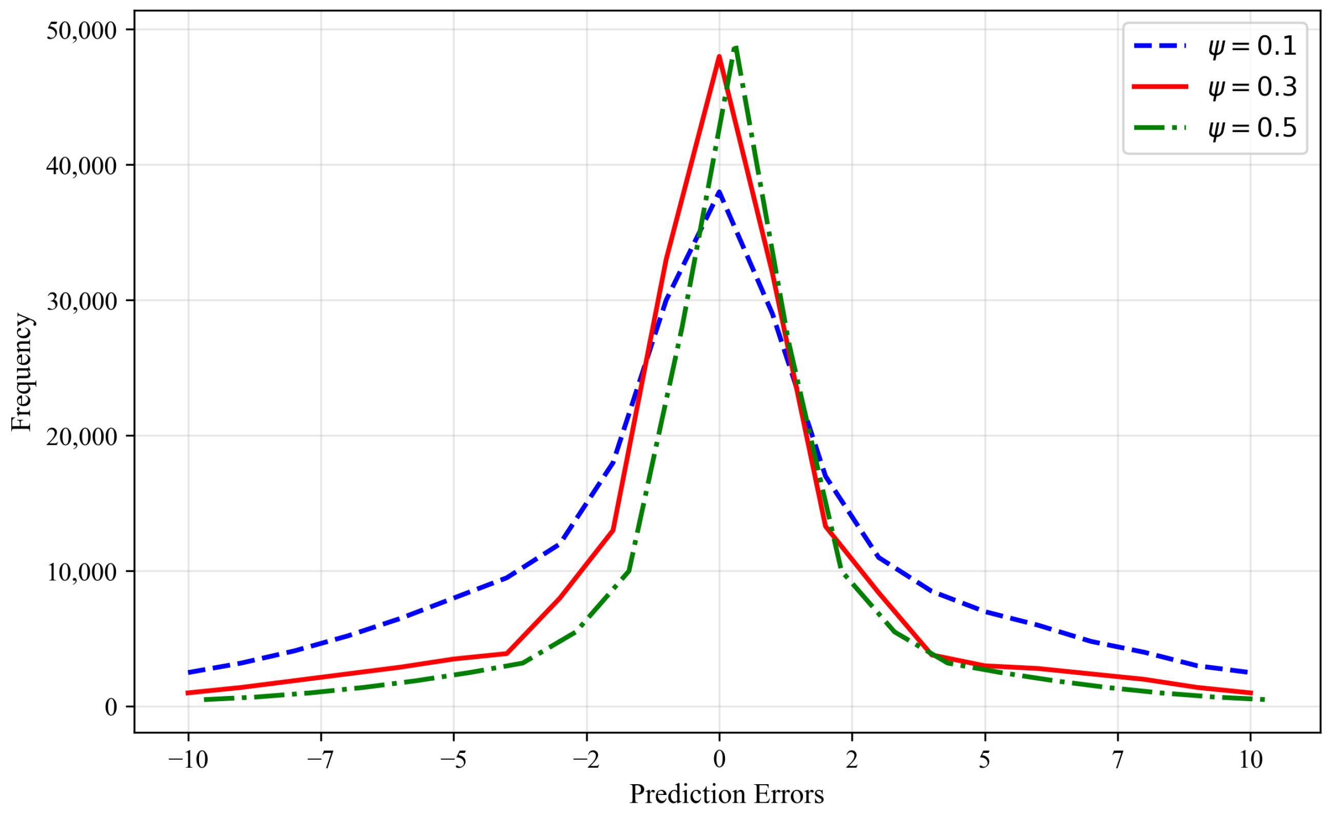
To demonstrate the variation of the prediction error histogram with the regularization term $\psi$, we plotted prediction error histograms for different values of $\psi$ as illustrated in Figure 11. For $\psi =0.1$, the prediction error histogram has a lower peak, and the tails are spread, indicating larger variance. As $\psi$ increases ($\psi =0.3$), the histogram distribution becomes more concentrated around zero. While a higher value ($\psi =0.5$) leads to a sharper and more concentrated error histogram, the peak shifts away from zero, which results in higher mean absolute error and consequently reduces the fidelity of the marked image.

Figure 11. Prediction error histogram variation with regularization parameter $\psi$.

To quantify the precision of the proposed AFCNNP, we have computed the number of zero-value prediction errors, where the predicted pixel value exactly matches the ground truth value, across all test images. As shown in Table 3, the proposed fusion method achieves a higher count of zero-value prediction errors compared to other methods; in particular, the zero-value prediction errors for the highly textured Baboon image are much higher than those of other methods. This is because the proposed method adaptively switches to NLM for predicting pixels in textured regions. The number of zero prediction errors is an indication of high-fidelity marked images after data embedding.

Table 3. Zero prediction error comparison between the proposed and existing predictors.

Image	Hu et al. [28]	Hu et al. [29]	Yang et al. [30]	Wu et al. [31]	Lin et al. [32]	Proposed
Lena	36,203	36,982	39,375	40,354	41,135	42,735
Baboon	12,032	12,940	13,765	14,011	15,322	16,371
Boat	22,111	25,078	27,550	28,428	30,352	31,142
Barbara	31,896	38,587	43,135	44,969	45,621	46,931
Pepper	21,959	23,807	28,038	29,600	32,199	33,753
Lake	20,409	23,101	25,934	26,246	26,832	27,926

3.2. Embedding Performance

In this section, we present extensive experimental results to prove the embedding performance of the proposed AFCNNP-based RDH method compared to existing RDH methods. Existing CNN-based RDH methods [28,29,30,31,32] have primarily focused on smooth regions or on minimizing prediction errors. While this strategy effectively generates sharply distributed prediction error histograms for RDH, resulting in low-distortion marked images, it results in selective data embedding excluding textured regions because of their higher and unpredictable prediction errors. Consequently, these methods may achieve low distortion but at the expense of reduced embedding capacity, particularly when working with complex images. In contrast, the proposed AFCNNP provides accurate prediction not only in smooth regions but also in textured regions, resulting in a broader pool of predictable pixels that are typically underutilized in prior approaches.

For fair comparison, we adopt the prediction error ordering (PEO) based RDH method with the proposed AFCNNP predictor and existing predictors. PEO enables adaptive sorting of pixels across the entire prediction error set, allowing balanced embedding across both smooth and textured regions. We performed experiments on 100 test images from the ucid.v2 dataset [41] and computed their average maximum embedding capacity and average PSNR at maximum embedding capacity for the proposed and existing methods as listed in Table 4. As shown in Table 4, the proposed AFCNNP-based RDH method better exploits textured regions of images to increase the embedding capacity and maintain high fidelity of the marked images. The average maximum embedding capacity of the proposed method is 125,816 bits, which is higher than that of all the existing methods. With a high embedding capacity (125,816), the average PSNR value of the proposed method (42.58 dB) is still above the nominal threshold.

Table 4. Comparison of RDH methods on texture utilization, average embedding capacity, and PSNR.

Method	Texture Utilization	Avg. Max Capacity (Bits)	Avg. PSNR at Max (dB)
Hu et al. [28]	Low	120,000	43.0
Hu et al. [29]	Low	45,000	52.1
Yang et al. [30]	Very Low	80,000	49.97
Wu et al. [31]	Low	20,000	59.64
Lin et al. [32]	Very Low	20,000	59.78
Proposed	Medium–High	125,816	42.58

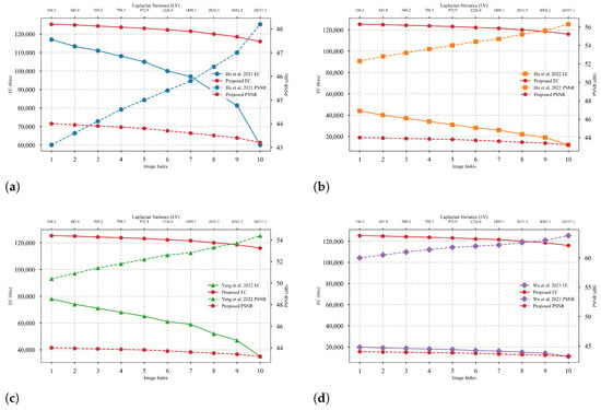
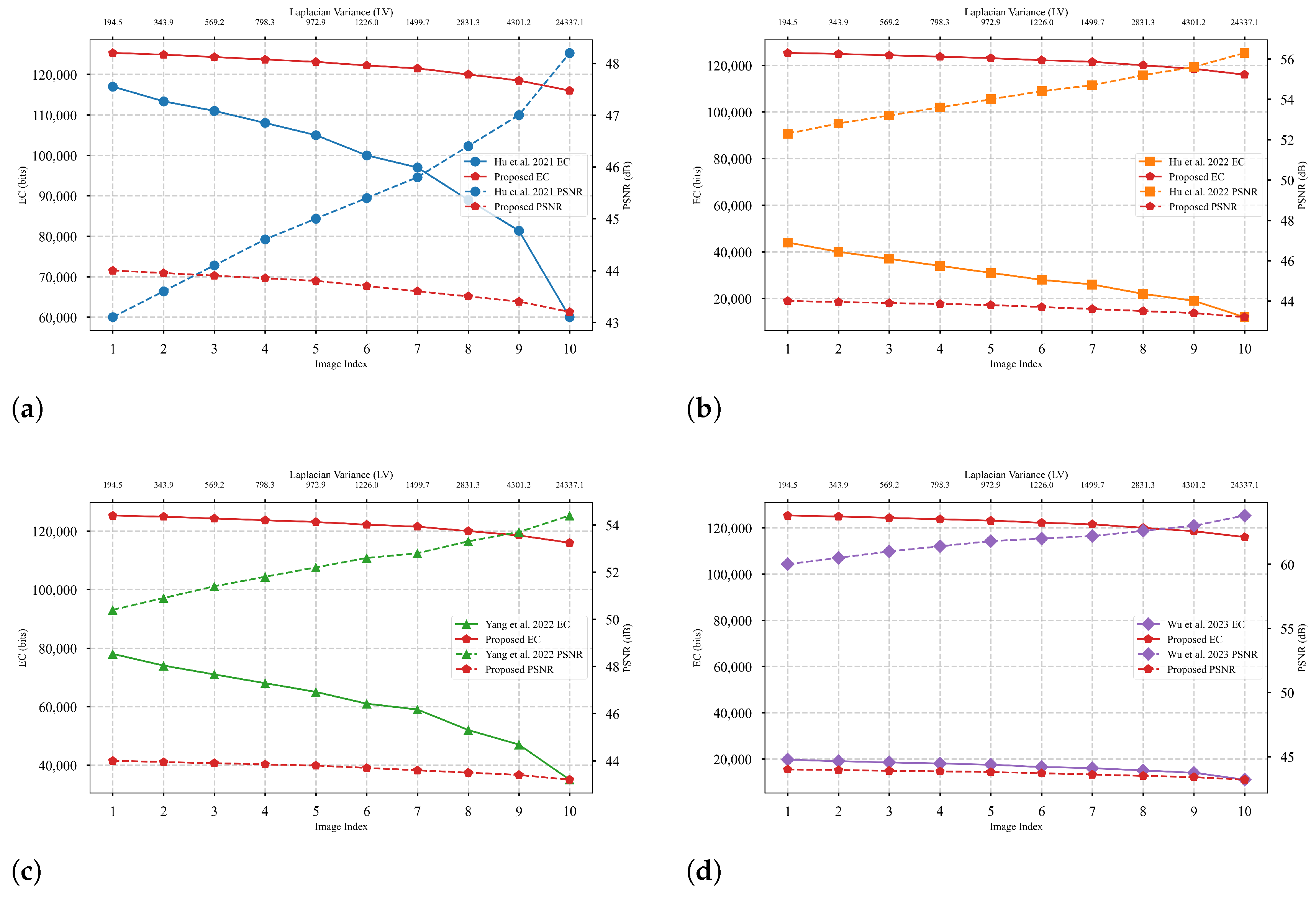
We conducted experiments on 10 images from the ucid.v2 dataset to investigate the relationship of embedding performance vs. image texture complexity for the proposed and existing methods. In the literature, various metrics are used to measure image texture complexity, such as local variance, Tamura Coarseness, entropy, spectral entropy, and Laplacian variance (LV). Here, we adopt LV as a measure of local texture and edge strength. The LV of all test images is computed, and then these images are sorted in ascending order of LV, effectively ranking them from smoother to textured images. For each image, the embedding capacity and PSNR values are computed using the proposed RDH method along with the existing RDH methods. These results are visualized in a dual-axis plot as shown in Figure 12, where the bottom x-axis represents the ordered image indices, the top x-axis represents LV values in ascending order, the left y-axis shows the embedding capacity, and the right y-axis displays the corresponding PSNR values. Figure 12 illustrates that existing methods that rely on local smoothness achieve low embedding capacities as texture increases. In contrast, our proposed method demonstrates stable or increasing embedding capacity in highly textured regions due to the inclusion of NLM predictions in such regions. This confirms the effectiveness of our attention-guided fusion strategy in leveraging structural redundancy beyond local smoothness, especially in complex textures.

Figure 12. Embedding performance comparison on texture complexity (a) Hu et al. [28] vs. Proposed, (b) Hu et al. [29] vs. Proposed, (c) Yang et al. [30] vs. Proposed, (d) Wu et al. [31] vs. Proposed.

Statistically, we have computed the average PSNR values for the proposed and existing RDH methods for 100 images using increasing embedding capacities from 10,000 bits to 20,000 bits with an increment of 1000 bits. These average PSNR values are listed in Table 5. When the embedding capacity is 10,000 bits, the average PSNR value of the proposed method is 65.50, which is higher than the values reported by Hu et al. [28] (63.42), Hu et al. [29] (64.12), Yang et al. [30] (64.32), Wu et al. [31] (65.03), and Lin et al. [32] (65.15). For the highest embedding capacity of 20,000 bits and intermediate embedding capacities, the PSNR values of the proposed method are still higher than those of the existing methods.

Table 5. Average PSNR of 100 test images for the proposed and existing predictors at various embedding capacities.

Bits	Hu et al. [28]	Hu et al. [29]	Yang et al. [30]	Wu et al. [31]	Lin et al. [32]	Proposed
10,000	63.42	64.12	64.32	65.03	65.15	65.50
11,000	63.18	63.62	63.79	64.71	64.89	65.17
12,000	62.89	63.41	63.50	64.35	64.51	64.80
13,000	62.51	63.02	63.10	64.01	64.13	64.45
14,000	62.21	62.76	62.73	63.63	63.78	64.06
15,000	61.89	62.50	62.41	63.22	63.43	63.65
16,000	61.56	62.21	62.09	62.91	63.06	63.30
17,000	61.31	61.93	61.80	62.56	62.74	62.95
18,000	61.12	61.70	61.61	62.40	62.58	62.78
19,000	60.89	61.49	61.40	62.21	62.32	62.59
20,000	60.67	61.27	61.15	61.94	61.98	62.30

To further evaluate the performance of the proposed AFCNNP-based RDH method, we conducted experiments on 10 images from the Kodak dataset [42]. These images from the Kodak dataset are color images of $512\times 768$ or $768\times 512$, which are converted to grayscale images and resized to $512\times 512$ size. Furthermore, we conducted ablation experiments. In Ablation 1, we computed the simple average of CNN and NLM predictions without the attention fusion network. Ablation 2 represents the embedding performance obtained without the variance regularization parameter used in Equation (12). Table 6 lists the PSNR values of the existing RDH methods, ablation results, and the proposed method on the Kodak images with an embedding capacity of 10,000 bits. As seen, the average PSNR value of the proposed method, 64.94, exceeds the methods of Hu et al. [28] (61.63), Hu et al. [29] (62.69), Yang et al. [30] (63.48), Wu et al. [31] (63.99), Lin et al. [32] (64.57), and both ablation results. These results prove the generalizability of the proposed method on diverse datasets.

Table 6. PSNR values of the existing and proposed RDH method on 10 Kodak images with an embedding capacity of 10,000 bits.

Image	Hu et al. [28]	Hu et al. [29]	Yang et al. [30]	Wu et al. [31]	Lin et al. [32]	Ablation 1	Ablation 2	Proposed
Kodak01	62.24	63.30	63.78	64.31	64.83	61.14	64.21	65.02
Kodak02	61.33	62.25	63.40	63.72	64.54	60.78	63.78	64.86
Kodak03	61.93	62.56	63.70	64.19	64.56	61.04	64.05	64.30
Kodak04	62.50	63.21	63.81	64.45	65.63	61.12	64.63	65.78
Kodak05	61.68	63.81	63.90	64.58	64.83	59.31	64.45	65.32
Kodak06	59.78	61.54	63.60	64.41	64.87	58.43	63.01	64.93
Kodak07	60.62	62.45	63.24	63.20	63.93	58.14	62.37	64.58
Kodak08	61.43	62.65	62.80	63.78	64.41	59.72	63.72	65.02
Kodak09	62.21	62.36	63.14	63.74	63.85	60.25	62.83	64.81
Kodak10	62.54	62.78	63.42	63.55	64.20	61.62	62.93	64.73
Average	61.63	62.69	63.48	63.99	64.57	60.15	63.59	64.94

To investigate the robustness and statistical significance of the proposed method, additional experiments were conducted on 24 images from the Kodak dataset. As mentioned earlier, these images were converted to grayscale and resized to $512\times 512$. For each existing CNN predictor and the proposed method, MSE and PSNR were computed over 24 images, and the mean and standard deviation were calculated. These results are shown in Table 7. As shown, the proposed method achieves lower MSE and higher mean PSNR compared to existing methods. For internal validation of the trained models, the standard deviations of performance metrics across the Kodak dataset were analyzed. The relatively lower standard deviation indicates that the proposed method achieves consistent prediction performance across diverse images.

Table 7. Statistical performance comparison on the Kodak dataset (24 images).

Method	MSE	PSNR
Hu et al. [28]	90.23 ± 4.2	60.42 ± 0.83
Hu et al. [29]	78.52 ± 3.7	61.51 ± 0.60
Yang et al. [30]	56.14 ± 3.4	63.23 ± 0.46
Wu et al. [31]	55.35 ± 3.1	63.67 ± 0.43
Lin et al. [32]	52.42 ± 2.8	64.12 ± 0.49
Proposed	50.30 ± 2.7	64.78 ± 0.38

To further verify the statistical significance of the observed improvement, we computed a paired t-test on the MSE values of the 24 images between the proposed method and the Lin et al. [32] method, which is superior among the existing methods. The test confirms that the performance gain of the proposed method is statistically significant ($p<0.05$), demonstrating that the improvements are consistent and not due to random variation.

3.3. Computational Complexity Analysis

To analyze the overall computational complexity of the proposed AFCNNP framework, we compute the complexities of the three components: the CNN predictor, the NLM predictor, and the attention fusion network. Let $H\times W$ be the size of the input image, and let $N=H\times W$ denote the total number of pixels in the image. The CNN predictor consists of three parallel feature extraction branches followed by a prediction branch. For a kernel size $K\times K$, input channels $C_{in}$, output channels $C_{out}$, each convolutional layer requires $\mathcal{O}(N\times K^2\times C_{in}\times C_{out})$. Each convolutional block in the feature extraction branch uses kernel sizes of $3\times 3$, $5\times 5$, and $7\times 7$ to produce 32 feature maps. The two convolutional blocks in series in the image prediction branch use a $3\times 3$ kernel size and produce 32 feature maps. The overall computational complexity of the CNN predictor is the sum of the costs of all convolutional blocks, which can be expressed as ${\mathcal{C}}_{CNN}=\mathcal{O}(6.7\times {10}^4\times N)$. The computational complexity of the CNN predictor is proportional to the image size.

The computational complexity of NLM predictor is given as ${\mathcal{C}}_{NLM}=\mathcal{O}(N\times S^2\times P^2)$, where $S\times S$ is the similarity search window size and $P\times P$ is the patch size. The overall complexity of the proposed predictor is dominated by the complexity of NLM. However, instead of a full image search, we use a localized search window, which significantly reduces the complexity of NLM. Here, we use $S=15$ and $P=5$, which results in ${\mathcal{C}}_{NLM}=\mathcal{O}(5.6\times {10}^3\times N)$. Due to the small search window size, the NLM complexity scales linearly with the image size.

As shown in Figure 5, the attention fusion module consists of two lightweight convolution layers ($2\to 16$ and $16\to 1$). The computational complexity of the attention fusion module is ${\mathcal{C}}_{Attn}=\mathcal{O}(4.3\times {10}^2\times N)$. The overall computational complexity of the proposed AFCNNP is the sum of the complexities of the CNN predictor, NLM predictor, and the attention fusion module, i.e., ${\mathcal{C}}_{total}={\mathcal{C}}_{CNN}+{\mathcal{C}}_{NLM}+{\mathcal{C}}_{Attn}$. Table 8 lists the computational complexities of the CNN predictor, the NLM predictor, the attention fusion module, and the overall computational complexity.

Table 8. Computational Complexity Analysis of the Proposed AFCNNP.

Component	Complexity
CNN Predictor	$\mathcal{O}(6.7\times {10}^4\times N)$
NLM Predictor	$\mathcal{O}(5.6\times {10}^3\times N)$
Attention Fusion Network	$\mathcal{O}(4.3\times {10}^2\times N)$
Total	$\mathcal{O}(7.3\times {10}^4\times N)$

4. Conclusions

Since pixels in smooth image regions are highly correlated, existing CNN predictors have primarily focused on generating prediction error histograms for these areas while down-weighting or ignoring textured regions, which tend to produce larger prediction errors. Although this approach effectively generates sharp, zero-centered prediction error histograms for reversible data hiding (RDH)—resulting in high-fidelity marked images—it restricts data embedding to smooth regions, leading to limited embedding capacity. In this paper, we propose a texture-aware attention fusion framework that combines a CNN predictor with an NLM predictor for accurate predictions in both smooth and textured regions of cover images. The attention fusion weight adaptively weighs the contributions from both predictors on a per-pixel basis, enabling accurate predictions across varying image complexities. We performed extensive experiments to demonstrate the superiority of the proposed predictor on diverse image datasets. The prediction error histogram generated by the proposed predictor is more concentrated around zero and more sharply distributed compared to those generated by existing CNN predictors, resulting in lower MAE, MSE, and variance. The number of zero-value prediction errors in the test images is also compared with existing predictors to demonstrate the precision of the proposed predictor. Furthermore, the proposed predictor is combined with the PEO-based RDH method, which achieved the highest embedding capacity compared to existing methods while maintaining high fidelity in the marked images.

In the future, we intend to adapt the NLM-based fusion framework by integrating it with a wider family of CNN predictors to achieve better texture-aware prediction and higher embedding capacity. We plan to investigate the proposed attention fusion framework in encrypted-domain RDH for privacy-preserving applications. We will also consider integrating transformer-based predictors into the proposed attention fusion framework in future research.

References

- Barton, J.M. Method and Apparatus for Embedding Authentication Information Within Digital Data. U.S. Patent 5,646,997, 8 July 1997. [Google Scholar]
- Shah, M.; Zhang, W.; Hu, H.; Dong, X.; Yu, N. Prediction error expansion-based reversible data hiding in encrypted images with public key cryptosystem. IET Image Process. 2019, 13, 1705–1713. [Google Scholar] [CrossRef] [Scilit]
- Ye, G.; Wu, H.; Liu, M.; Huang, X. Reversible image-hiding algorithm based on singular value sampling and compressive sensing. Chaos Solitons Fractals 2023, 171, 113469. [Google Scholar] [CrossRef] [Scilit]
- Bhatnagar, G.; Wu, Q.J.; Atrey, P.K. Secure randomized image watermarking based on singular value decomposition. ACM Trans. Multimed. Comput. Commun. Appl. (TOMM) 2013, 10, 4. [Google Scholar] [CrossRef] [Scilit]
- Naskar, R.; Chakraborty, R.S. A generalized tamper localization approach for reversible watermarking algorithms. ACM Trans. Multimed. Comput. Commun. Appl. (TOMM) 2013, 9, 19. [Google Scholar] [CrossRef] [Scilit]
- Shah, M.; Zhang, W.; Hu, H.; Zhou, H.; Mahmood, T. Homomorphic encryption-based reversible data hiding for 3D mesh models. Arab. J. Sci. Eng. 2018, 43, 8145–8157. [Google Scholar] [CrossRef] [Scilit]
- Hu, R.; Xiang, S. Cover-lossless robust image watermarking against geometric deformations. IEEE Trans. Image Process. 2020, 30, 318–331. [Google Scholar] [CrossRef] [Scilit]
- Xiong, L.; Han, X.; Yang, C.N.; Xia, Z. RDH-DES: Reversible data hiding over distributed encrypted-image servers based on secret sharing. ACM Trans. Multimed. Comput. Commun. Appl. 2023, 19, 5. [Google Scholar] [CrossRef] [Scilit]
- Zhang, X. Separable reversible data hiding in encrypted image. IEEE Trans. Inf. Forensics Secur. 2011, 7, 826–832. [Google Scholar] [CrossRef] [Scilit]
- Coatrieux, G.; Le Guillou, C.; Cauvin, J.M.; Roux, C. Reversible watermarking for knowledge digest embedding and reliability control in medical images. IEEE Trans. Inf. Technol. Biomed. 2008, 13, 158–165. [Google Scholar] [CrossRef] [Scilit] [PubMed]
- Gao, G.; Tong, S.; Xia, Z.; Wu, B.; Xu, L.; Zhao, Z. Reversible data hiding with automatic contrast enhancement for medical images. Signal Process. 2021, 178, 107817. [Google Scholar] [CrossRef] [Scilit]
- Horng, J.H.; Chang, C.C.; Li, G.L.; Lee, W.K.; Hwang, S.O. Blockchain-based reversible data hiding for securing medical images. J. Healthc. Eng. 2021, 2021, 9943402. [Google Scholar] [CrossRef] [Scilit] [PubMed]
- Fridrich, J.; Goljan, M.; Du, R. Lossless data embedding for all image formats. In Proceedings of the Security and Watermarking of Multimedia Contents IV; SPIE: Bellingham, WA USA, 2002; Volume 4675, pp. 572–583. [Google Scholar]
- Zhang, W.; Hu, X.; Li, X.; Yu, N. Recursive histogram modification: Establishing equivalency between reversible data hiding and lossless data compression. IEEE Trans. Image Process. 2013, 22, 2775–2785. [Google Scholar] [CrossRef] [Scilit] [PubMed]
- Celik, M.U.; Sharma, G.; Tekalp, A.M.; Saber, E. Lossless generalized-LSB data embedding. IEEE Trans. Image Process. 2005, 14, 253–266. [Google Scholar] [CrossRef] [Scilit]
- Tian, J. Reversible data embedding using a difference expansion. IEEE Trans. Circuits Syst. Video Technol. 2003, 13, 890–896. [Google Scholar] [CrossRef] [Scilit]
- Ni, Z.; Shi, Y.Q.; Ansari, N.; Su, W. Reversible data hiding. IEEE Trans. Circuits Syst. Video Technol. 2006, 16, 354–362. [Google Scholar] [PubMed]
- Zhang, T.; Li, X.; Qi, W.; Guo, Z. Prediction-error value ordering for high-fidelity reversible data hiding. In Proceedings of the International Conference on Multimedia Modeling; Springer: Cham, Switzerland, 2019; pp. 317–328. [Google Scholar]
- Qin, J.; Huang, F. Reversible data hiding based on prediction-error-ordering. In Proceedings of the Chinese Conference on Pattern Recognition and Computer Vision (PRCV); Springer: Cham, Switzerland, 2020; pp. 527–537. [Google Scholar]
- Thodi, D.M.; Rodríguez, J.J. Expansion embedding techniques for reversible watermarking. IEEE Trans. Image Process. 2007, 16, 721–730. [Google Scholar] [CrossRef] [Scilit]
- Sachnev, V.; Kim, H.J.; Nam, J.; Suresh, S.; Shi, Y.Q. Reversible watermarking algorithm using sorting and prediction. IEEE Trans. Circuits Syst. Video Technol. 2009, 19, 989–999. [Google Scholar] [CrossRef] [Scilit]
- Coltuc, D. Low distortion transform for reversible watermarking. IEEE Trans. Image Process. 2011, 21, 412–417. [Google Scholar] [CrossRef] [Scilit]
- Ou, B.; Li, X.; Zhao, Y.; Ni, R. Reversible data hiding based on PDE predictor. J. Syst. Softw. 2013, 86, 2700–2709. [Google Scholar] [CrossRef] [Scilit]
- Dragoi, I.C.; Coltuc, D. Local-prediction-based difference expansion reversible watermarking. IEEE Trans. Image Process. 2014, 23, 1779–1790. [Google Scholar] [CrossRef] [Scilit]
- Jafar, I.F.; Darabkh, K.A.; Al-Zubi, R.T.; Al Na’mneh, R.A. Efficient reversible data hiding using multiple predictors. Comput. J. 2016, 59, 423–438. [Google Scholar] [CrossRef] [Scilit]
- Hong, I.; Choi, C. Knowledge distillation vulnerability of DeiT through CNN adversarial attack. Neural Comput. Appl. 2025, 37, 7721–7731, Correction in Neural Comput. Appl. 2025, 37, 21347. [Google Scholar] [CrossRef] [Scilit]
- Wang, T.; Li, J.; Zhang, M.; Zhu, A.; Snoussi, H.; Choi, C. An enhanced 3DCNN-ConvLSTM for spatiotemporal multimedia data analysis. Concurr. Comput. Pract. Exp. 2021, 33, e5302. [Google Scholar] [CrossRef] [Scilit]
- Hu, R.; Xiang, S. CNN prediction based reversible data hiding. IEEE Signal Process. Lett. 2021, 28, 464–468. [Google Scholar] [CrossRef] [Scilit]
- Hu, R.; Xiang, S. Reversible data hiding by using CNN prediction and adaptive embedding. IEEE Trans. Pattern Anal. Mach. Intell. 2022, 44, 10196–10208. [Google Scholar] [CrossRef] [Scilit] [PubMed]
- Yang, X.; Huang, F. New CNN-based predictor for reversible data hiding. IEEE Signal Process. Lett. 2022, 29, 2627–2631. [Google Scholar] [CrossRef] [Scilit]
- Wu, M.; Xiang, S. An Efficient CNN-based Prediction for Reversible Data Hiding. In Proceedings of the 5th ACM International Conference on Multimedia in Asia, Tainan, Taiwan, 6–8 December 2023; pp. 1–5. [Google Scholar]
- Lin, M.; Xiang, S. Efficient CNN Prediction with Smoothness Factor for Reversible Data Hiding. IEEE Signal Process. Lett. 2025, 32, 1341–1345. [Google Scholar] [CrossRef] [Scilit]
- Qiu, Y.; Peng, W.; Lin, X. Improved CNN prediction based reversible data hiding for images. Entropy 2025, 27, 159. [Google Scholar] [CrossRef] [Scilit]
- Zhao, Y.; Peng, Y.; Fang, Y.; Zhang, T.; Wang, J. CNN-Based Hybrid Prediction Scheme for Image Reversible Data Hiding. Circuits Syst. Signal Process. 2025, 45, 2261–2286. [Google Scholar] [CrossRef] [Scilit]
- Fan, G.; Zuo, C.; Lu, L.; Yang, Z.; Zhao, J.; Pan, Z. PVO-based reversible data hiding with flexible strip moving using classification-based adaptive prediction guided by CNN. J. Inf. Secur. Appl. 2026, 97, 104368. [Google Scholar] [CrossRef] [Scilit]
- Duan, H.; Tao, Z.; Ma, B.; Xu, J.; Xian, Y. High Precision CNN Predictor of Color Images for Reversible Data Hiding. IEEE Signal Process. Lett. 2025, 32, 3859–3863. [Google Scholar] [CrossRef] [Scilit]
- Zhou, L.; Lu, Z.; You, W.; Fang, X. Reversible data hiding using a transformer predictor and an adaptive embedding strategy. Front. Inf. Technol. Electron. Eng. 2023, 24, 1143–1155. [Google Scholar] [CrossRef] [Scilit]
- Deng, J.; Dong, W.; Socher, R.; Li, L.J.; Li, K.; Li, F.-F. Imagenet: A large-scale hierarchical image database. In Proceedings of the 2009 IEEE Conference on Computer Vision and Pattern Recognition; IEEE: Piscataway, NJ, USA, 2009; pp. 248–255. [Google Scholar]
- Kingma, D.P.; Ba, J.L. Adam: A method for stochastic optimization. In Proceedings of the International Conference on Learning Representations, San Diego, CA, USA, 7–9 May 2015; pp. 1–15. [Google Scholar]
- LeCun, Y.; Bottou, L.; Bengio, Y.; Haffner, P. Gradient-based learning applied to document recognition. Proc. IEEE 2002, 86, 2278–2324. [Google Scholar] [CrossRef] [Scilit]
- Schaefer, G.; Stich, M. UCID: An uncompressed color image database. In Proceedings of the Storage and Retrieval Methods and Applications for Multimedia 2004; SPIE: Bellingham, WA USA, 2003; Volume 5307, pp. 472–480. [Google Scholar]
- Franzen, R. Kodak Lossless True Color Image Suite. 1999. Available online: https://r0k.us/graphics/kodak/ (accessed on 20 March 2026).
Disclaimer/Publisher’s Note: The statements, opinions and data contained in all publications are solely those of the individual author(s) and contributor(s) and not of MDPI and/or the editor(s). MDPI and/or the editor(s) disclaim responsibility for any injury to people or property resulting from any ideas, methods, instructions or products referred to in the content. |
© 2026 by the authors. Licensee MDPI, Basel, Switzerland. This article is an open access article distributed under the terms and conditions of the Creative Commons Attribution (CC BY) license.