


Abstract
This study examines the distances between consecutive generalized zeros of first-order difference equations with several variable delays. We develop new techniques to obtain the upper bounds for these distances. The results are not only new, but they also extend and improve several earlier contributions in this area. In particular, our analysis covers the case of nonmonotonic delay sequences, which, to the best of our knowledge, has not been previously investigated, even for the corresponding delay differential equations. To illustrate the effectiveness of our findings, three numerical examples will be presented.
Keywords:
difference equations; differential equations; general delays; generalized zeros; oscillatory behavior MSC:
34K11; 39A21; 34C10
1. Introduction
Consider the first-order difference equation with several variable delays
and the following special cases:
and
where , are nonnegative numbers; are positive integers; for are sequences of nonnegative real numbers; and are sequences of integers such that
A solution to Equation (1) refers to a sequence of real numbers , where that satisfies Equation (1) for all . It is evident that for any selection of real numbers , there exists a unique solution that meets the initial conditions . This solution is termed oscillatory if all elements of the sequence are neither eventually positive nor negative; otherwise, it is called non-oscillatory. Equation (1) is considered oscillatory if all its solutions are oscillatory, while it is termed non-oscillatory if it has at least one non-oscillatory solution.
We will rearrange Equations (1) and (2) to ensure that the following conditions are satisfied:
and
respectively.
The study of delay difference equations has gained significant momentum due to their ability to describe complex phenomena in discrete time, which is the natural framework for digital computing, population dynamics with seasonal breeding, and sampled-data control systems (see [1,2,3,4,5,6,7,8,9]). While delay differential equations provide a continuous perspective, their discrete counterparts offer a more direct approach for numerical implementations and recursive modeling. Understanding the spacing between the zeros of these solutions is not only a theoretical challenge but also a practical necessity for assessing the stability and oscillatory frequency of systems subject to propagation delays.
Over the past few years, there has been a noticeable increase in the study of oscillations in delay difference equations, primarily because many natural models exhibit such behavior (see [10,11,12]). This interest parallels that in the study of the same property for the corresponding delay differential equations (see [13,14,15]). However, the study of the distance between generalized zeros of delay difference equations (DGZ-DDEs) has not received comparable attention.
In contrast, the distance between zeros of solutions to delay differential equations has attracted significant attention. For example, first-order differential equations with a single delay were examined in [16,17,18,19,20], while equations with several delays were studied in [21,22]. In addition, first-order neutral differential equations were investigated in [23,24,25,26].
Recently, the study of DGZ-DDEs has received significant attention, with numerous direct investigations devoted to this topic; see, for example [27,28,29,30]. In these works, the delays are typically assumed to be constant, that is, . In more general settings, the delays are not necessarily monotone increasing, but they are still bounded above by constant delays, i.e., . On the other hand, several authors have examined related problems by studying the distribution of zeros for broader classes of equations that unify discrete and continuous frameworks. These equations are commonly referred to as dynamic equations on time scales; see, for instance [28,31,32,33]. However, to our knowledge, Equation (1), which incorporates general (nonconstant and unbounded) delays, has not yet been investigated in the literature.
In this paper, we introduce iterative functional techniques to establish lower and upper bounds for the ratio , and we employ these bounds to investigate DGZ-DDE for all solutions of Equation (1). To this end, we extend and refine the existing methods used to study the distances between the zeros of first-order delay differential equations.
We establish several new upper bounds for DGZ-DDE of the form (1), which not only generalize but also improve previously known results for important special cases of this equation. To demonstrate the applicability of our results, we present two illustrative examples that highlight the effectiveness of our conditions in predicting oscillatory behavior and determining the locations of generalized zeros of the solutions. Moreover, a comparison with previously known results shows that they do not yield comparable approximations.
2. Main Results
Let be the maximum positive integer such that for every with , and for every solution of a difference equation E, the elements , must change their sign, or be equal to zero, at least two times.
By , we mean that all nonnegative integers belong to the interval .
Let . The following notation will be used:
It is important to note that the sequences satisfy the following inequality:
Furthermore, if , then it follows that . Consequently, we have , which implies that for .
Similarly, if , it can be deduced that , leading to for .
Also, for , let the sequence be defined by and
Lemma 1.
Proof.
Since on , it follows from (1) that
and hence is nonincreasing on . Therefore,
and
Dividing Equation (1) by , and then taking the product, from u to , , we get
that is,
This together with (8) leads to
and
for . From (10) and (11), we obtain
Then
and
By repeating the arguments stated above, we derive (6) and (7). □
Let
and
To justify that is well-defined, we note that by assumption
Hence, for any fixed , there exists such that
Therefore, the set
is nonempty, and since it is a subset of , it admits a minimum element. Consequently, is well-defined. Moreover, since for all , it follows that
We also define the sequences for as follows:
Lemma 2.
Proof.
Summing up Equation (1) for , we obtain
for . We will demonstrate the following:
- 1.
- 2.
- For ,
To prove the first claim, assume that , so , and hence . This shows that meets the criteria for being one of the integers included in the definition of ; therefore,
Thus, the first statement has been established.
For the second claim, we first show that . Suppose, on the contrary, that there exists such that . Therefore,
In view of the definition of , it follows that . This contradicts the assumption that . Therefore, . To complete the proof of the second statement, we still need to demonstrate that . We will clarify this as follows:
Since , it follows that , which implies . According to the definition of , we have ; thus, .
Using the fact that and the definition of the sequences and , we can prove that
This, along with (16), leads to
Next, we demonstrate that
Assuming the contrary, let us suppose that . This implies that . According to the definition of , it follows that . This leads to a contradiction, thereby proving that .
Furthermore, for , it can be readily established that . Therefore, is non-increasing. Using (18), we have
From this and (17), we obtain
Substituting into (15) and rearranging, it follows that
for
By iterating this procedure l times, we obtain (12). □
Theorem 1.
Let be the smallest positive integer such that is negative or undefined, and l be the smallest nonnegative integer that satisfies
and are the smallest positive integers such that
Moreover, if
then
Proof.
Let be a positive solution of Equation (1) on . Then, Lemmas 1 and 2 imply, respectively,
and
Therefore, for , we have
This contradiction concludes the proof of the first part. Now, let us assume that is a positive solution of Equation (1) on the interval , where . In this case, Lemma 1 implies that
This contradicts the definition of . Therefore, any solution has at least one generalized zero in any interval of the forms and . To complete the proof, let us assume the existence of a positive integer such that and . Using the same method of the proof as before, we can prove that changes its sign (or is equal to zero) in and in . Then, changes its sign (or equal to zero) at least twice in and in . □
In the following, we assume that is non-decreasing for .
Let and the sequence , be defined by
Theorem 2.
If
then
Proof.
Suppose the opposite, and let for , where . We first demonstrate that cannot remain positive on the interval . It follows from Equation (1) that
Summing up from r to , we get
Then,
In view of , it follows from the non-decreasing natural of that for , . Again, Equation (21), yields
From (22) and (23), we obtain
for , that is,
for . Since , for . It follows from (21) that
Substituting into (24), we have
for Therefore,
where . By using the positivity of , we obtain
Following l iterations of this argument, we arrive at
Clearly
It can be inferred from , that . This, in conjunction with Equation (6), results in
Substituting into (28), we obtain
This, together with (27), leads to
for .
This contradiction demonstrates that cannot be positive on the interval . To finalize the proof, we can show that any solution has at least two generalized zeros in the interval by applying the same method used at the conclusion of the proof of Theorem 1. □
Theorem 3.
If
then
Proof.
Let be a positive solution of Equation (1) on , . First, we clarify that cannot remain positive over the interval . Summing up Equation (1) from to , where , we get
Using (10) and for , the last equation takes the form
for . From (7) and the positivity of we have
for . Using the arithmetic–geometric mean, we get
for . Taking the product of both sides
for . That is,
Contradicting (30), the rest of the proof is similar to the ends of the proofs of Theorems 1 and 2. Thus, the proof is complete. □
Let , , and , where .
Corollary 1.
Assume that .
- (i)
- If , then .
- (ii)
- Ifthen
Proof.
Assume that , , . At the beginning, we will calculate some sequences that we need to obtain the result. Clearly
and
Furthermore,
and
In view of , it follows that is not defined. By applying Theorem 1 with , we obtain
Thus, the proof of (i) is complete.
Corollary 2.
- (i)
- If , then .
- (ii)
- Ifthen .
Corollary 3.
- (i)
- If , then .
- (ii)
- Ifthen .
Proof.
Using the same method as in the proof of Corollary 1, we obtain
Applying Theorem 2 with , it follows that
The proof of (i) is complete.
Let
Clearly,
Therefore,
Then
Since all the requirements of Theorem 2 with are fulfilled, then . The proof is complete. □
Corollary 4.
- (i)
- If , then .
- (ii)
- Ifthen .
Remark 1.
The sequences and are defined iteratively through positive quantities under the standing assumptions on the coefficients .
First, since and , it follows that for all , provided that
which ensures that the product defining is well-defined. Moreover, as l increases, the term typically increases, which makes each factor
larger, and hence the lower bound on becomes larger.
Similarly, the sequence is well-defined and positive whenever
Moreover, the sequence is nonincreasing in l and hence bounded. Consequently, there exists an index such that
which shows that the sequence eventually dominates as l increases.
3. Numerical Examples
In this section, we present three numerical examples that illustrate the applicability of our results. The first example considers a case where the delays are neither monotonic nor comparable (i.e., is not consistently positive or negative). This scenario poses significant challenges in determining the distance between zeros. The second example focuses on analyzing the distance between zeros in a single-delay equation where the delay is nonmonotone and unbounded. In the final example, we show that the error in our estimate is less than twice the delay.
Example 1.
Consider the first-order difference equation
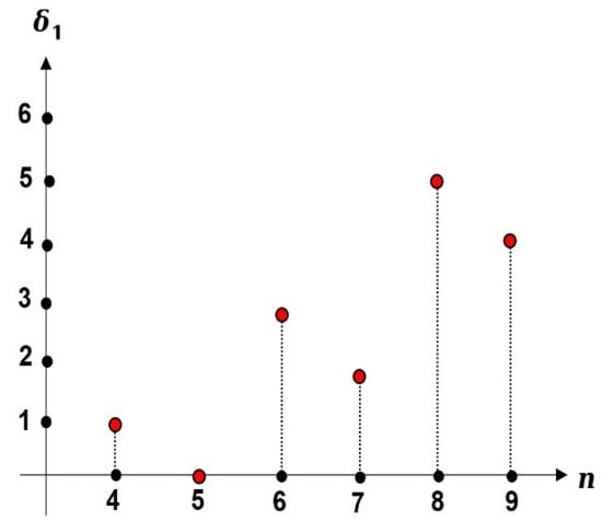
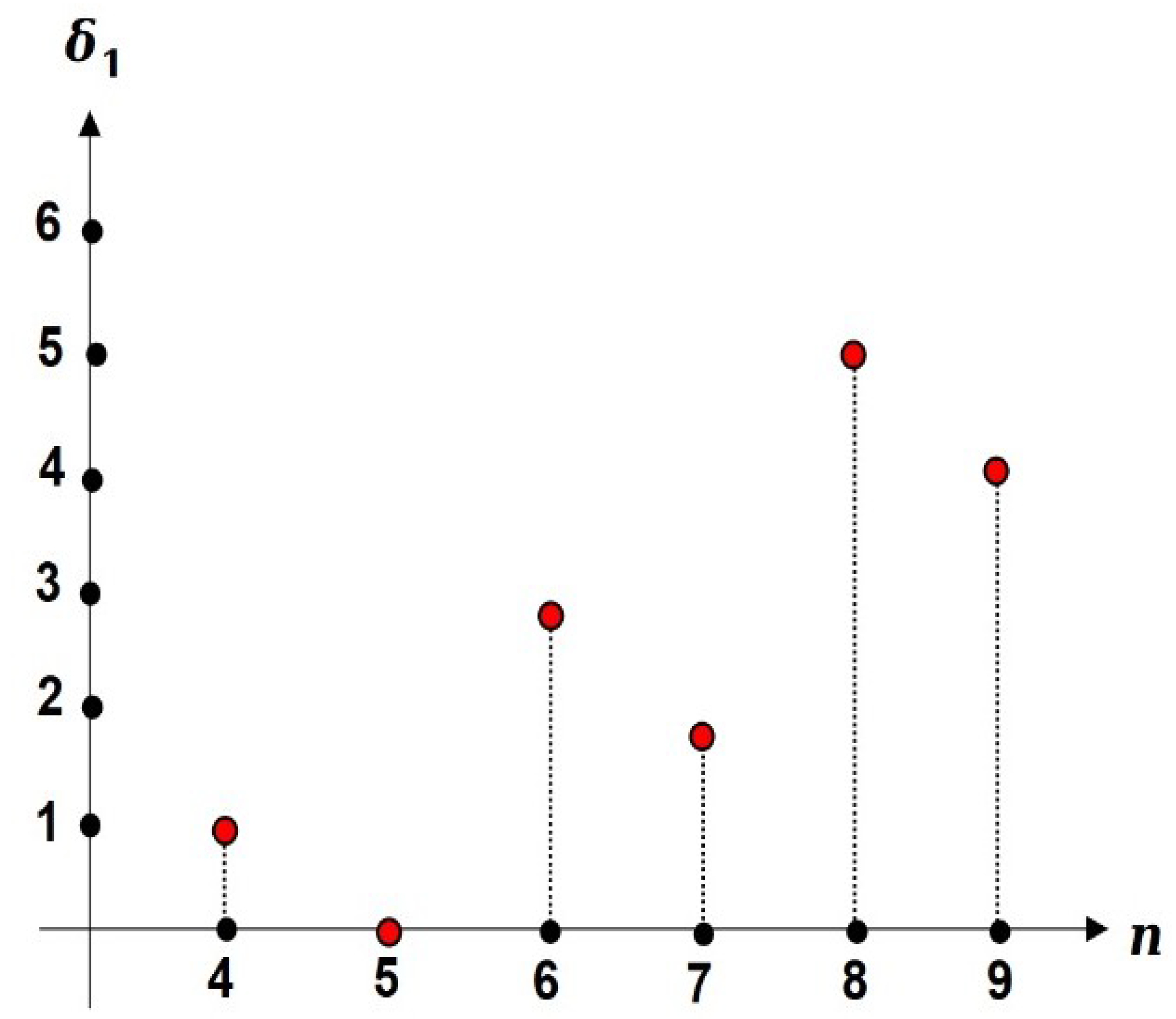
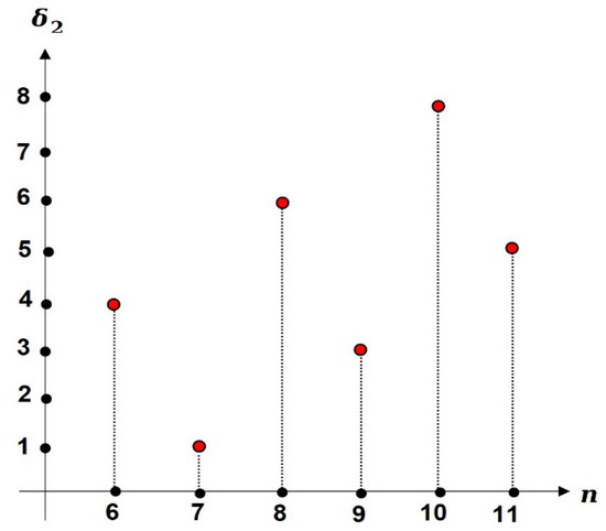
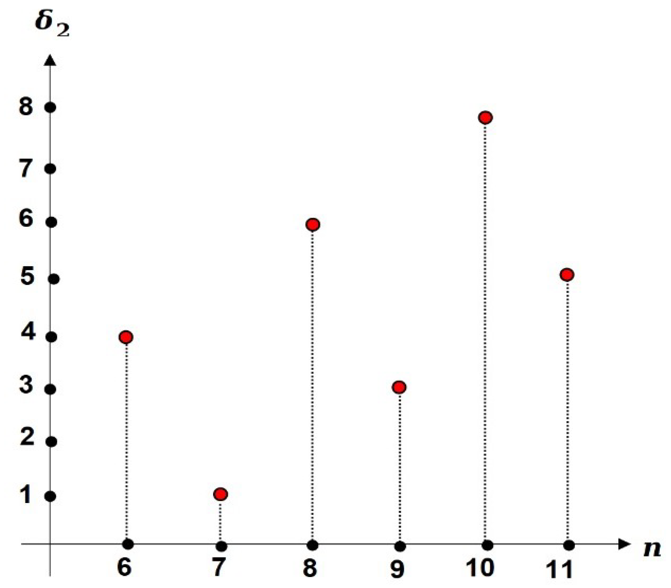
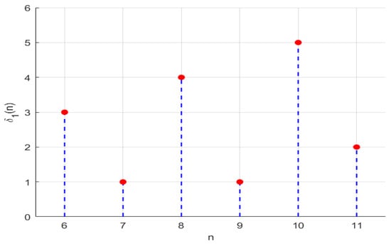
where , and
and
Figure 1.
The graph of the sequence .
Figure 2.
The graph of the sequence .
Clearly
and
Then, Condition (5) is satisfied. Clearly, , and
and
Therefore,
and
Consequently,
Furthermore,
and
Hence
Assume that . Therefore,
Accordingly, it is feasible to choose
Let
Then
As a result, one may select
Then
Since
and
it follows that . Consequently, Theorem 1 with and implies that
It should be emphasized that, to the best of the authors’ knowledge, the DGZ-DDE of (35), have not been previously investigated, especially in the case of non-monotonic delays.
Example 2.
Consider the first-order difference equation
where
where is the Floor function. This equation has the form of (1) with and .
To illustrate the non-monotone behavior of the sequence , we present its graph in Figure 3.
Figure 3.
The graph of the sequence .
Clearly,
Next, we estimate . By definition,
it follows that
Similarly,
Hence,
and, by induction,
In the same way,
and
In view of the fact that , it follows that is undefined.
Consequently, by Theorem 1 with and , every solution of (36) has at least one zero in the interval
It is worth noting that the previous criteria are not applicable to this example due to the non-monotonic nature of the delay, which is also not bounded above by a constant delay. More precisely, there does not exist such that . Indeed, most existing methods rely essentially on these two assumptions. This highlights the significance of our results, which do not require monotonicity and are therefore capable of handling a broader class of delay difference equations.
Example 3.
Consider the first-order difference equation
where
where .
Below, we will calculate the left-hand side of Condition (19) for Equation (37) when , and 4, respectively.
and
By applying Theorem 2, we obtain the distance between consecutive zeros for all solutions of Equation (37) for different values of the parameter a, as shown in Table 1.
Table 1.
This table shows the relationship between the distance between consecutive zeros of all solutions of Equation (37) and the parameter a.
However, none of the results reported in [27,29] provide estimates that are sharper than those obtained in Table 1. A direct comparison based on Table 1 and Table 2 clearly illustrates this improvement.
Table 2.
Upper bounds on the distance between consecutive generalized zeros of all solutions of Equation (37) obtained in earlier works for various ranges of the parameter a.
For instance, for , our result gives an upper bound equal to 4, which improves the bound 6 in [27] and coincides with the best bound 4 in [29]. Moreover, for , we obtain the bound 5, which is strictly better than the bound 6 in [27,29].
In addition, for , our estimate does not exceed 5, which improves the bound 6 in [27,29]. Furthermore, for smaller values of a, our results yield bounds such as 6 and 7, whereas the existing results in [27,29] are unable to attain such bounds for the same ranges of the parameter a.
These comparisons confirm that the bounds obtained in this work are consistently smaller or equal to those in the existing literature. Since a smaller upper bound corresponds to a more accurate estimation of the distance between consecutive generalized zeros, this demonstrates the effectiveness and superiority of our results.
It is noteworthy that the specific case of Equation (37), given by
with the initial conditions , possesses the solutions , , and . Consequently, the upper bound on the distance between the generalized zeros of all solutions of Equation (38) is greater than 2. However, as indicated in Table 1, this upper bound is not greater than 4. Therefore, we can conclude that our estimation error is less than 2.
4. Conclusions
In this work, we studied DGZ-DDE with several variable delays. We not only improved and generalized some methods used to examine the distance between zeros, but we also investigated this property in cases of non-monotone delays (as far as the authors are aware, the distribution of zeros for first-order differential equations with non-monotone delay has not been studied before). We obtained several new approximations for the distance between zeros. The methods employed in this work can also be used to study the oscillation and the distance between the zeros of many other equations, such as first-order neutral difference equations and higher-order delay differential equations, which are commonly employed to model various natural phenomena.
Author Contributions
Methodology, E.A., A.A., G.C. and B.E.-M.; Formal analysis, E.A.; Investigation, E.A., A.A., G.C. and B.E.-M.; Writing—original draft, E.A., G.C. and B.E.-M.; Writing—review and editing, E.A., G.C. and B.E.-M.; Supervision, G.C. All authors have read and agreed to the published version of the manuscript.
Funding
The authors extend their appreciation to Prince Sattam bin Abdulaziz University for funding this research work through the project number (PSAU/2025/01/34352).
Data Availability Statement
The original contributions presented in this study are included in the article. Further inquiries can be directed to the corresponding author.
Acknowledgments
The authors extend their appreciation to Prince Sattam bin Abdulaziz University for funding this research work through the project number (PSAU/2025/01/34352).
Conflicts of Interest
The authors declare no conflict of interest.
References
- Agarwal, R.P.; Berezansky, L.; Braverman, E.; Domoshnitsky, A. Non-Oscillation Theory of Functional Differential Equations with Applications; Springer: New York, NY, USA, 2012. [Google Scholar]
- Agarwal, R.P.; Grace, S.R.; O’Regan, D. Oscillation Theory for Difference and Functional Differential Equations; Springer Science and Business Media: Dordrecht, The Netherlands, 2013. [Google Scholar]
- Ahmed, N.; Elsonbaty, A.; Adel, W.; Baleanu, D.; Rafiq, M. Stability analysis and numerical simulations of spatiotemporal HIV CD4+ T cell model with drug therapy. Chaos 2020, 30, 083145. [Google Scholar] [CrossRef] [Scilit]
- Al-khedhairi, A.; Elsadany, A.A.; Elsonbaty, A. Modelling immune systems based on Atangana–Baleanu fractional derivative. Chaos Solitons Fractals 2019, 129, 25–39. [Google Scholar] [CrossRef] [Scilit]
- Erbe, L.H.; Kong, Q.; Zhang, B.G. Oscillation Theory for Functional Differential Equations; Dekker: New York, NY, USA, 1995. [Google Scholar]
- Ghosh, D.; Santra, P.K.; Mahapatra, G.S.; Elsonbaty, A.; Elsadany, A.A. A discrete-time epidemic model for the analysis of transmission of COVID19 based upon data of epidemiological parameters. Eur. Phys. J. Spec. Top. 2022, 231, 3461–3470. [Google Scholar] [CrossRef] [Scilit] [PubMed]
- Gopalsamy, K. Stability and Oscillation in Delay Differential Equations of Population Dynamics; Kluwer Academic Publishers: Dordrecht, The Netherlands; Boston, MA, USA; London, UK, 1992. [Google Scholar]
- Gyori, I.; Ladas, G. Oscillation Theory of Delay Differential Equations with Applications; Clarendon Press: Oxford, UK, 1991. [Google Scholar]
- Sharma, V.S.; Singh, A.; Elsonbaty, A.; Elsadany, A.A. Codimension-one and -two bifurcation analysis of a discrete-time prey-predator model. Int. J. Dyn. Control 2023, 11, 2691–2705. [Google Scholar] [CrossRef] [Scilit]
- El-Matary, B.M.; El-Morshedy, H.A.; Benekas, V.; Stavroulakis, I.P. Oscillation conditions for difference equations with several variable delays. Opusc. Math. 2023, 43, 789–801. [Google Scholar] [CrossRef] [Scilit]
- El-Morshedy, H.A. New oscillation criteria for second order linear difference equations with positive and negative coefficients. Comput. Math. Appl. 2009, 58, 1988–1997. [Google Scholar] [CrossRef] [Scilit]
- Grace, S.R.; El-Morshedy, H.A. Oscillation criteria of comparison type for second order difference equations. J. Appl. Anal. 2000, 6, 87–102. [Google Scholar] [CrossRef] [Scilit]
- Barr, T.H. Oscillations in linear delay differential equations. J. Math. Anal. Appl. 1995, 195, 261–277. [Google Scholar] [CrossRef] [Scilit]
- Elbert, A.; Stavroulakis, I.P. Oscillation of first order differential equations with deviating arguments. In Recent Trends in Differential Equations; World Scientific: River Edge, NJ, USA, 1992; Volume 1, pp. 163–178. [Google Scholar]
- Jaroš, J.; Stavroulakis, I.P. Oscillation tests for delay equations. Rocky Mt. J. Math. 1999, 29, 197–207. [Google Scholar] [CrossRef] [Scilit]
- El-Morshedy, H.A. On the distribution of zeros of solutions of first order delay differential equations. Nonlinear Anal. 2011, 74, 3353–3362. [Google Scholar] [CrossRef] [Scilit]
- Tang, X.H.; Yu, J.S. Distribution of zeros of solutions of first order delay differential equations. Appl. Math. J. Chin. Univ. Ser. B 1999, 14, 375–380. [Google Scholar]
- Tang, X.H.; Yu, J.S. The Maximum Existence Interval of Positive Solutions of First Order Delay Differential Inequalities with Applications. Math. Pract. Theory 2000, 30, 447–452. [Google Scholar]
- Wu, H.W.; Erbe, L. On the distance between consecutive zeros of solutions of first order delay differential equations. Appl. Math. Comput. 2013, 219, 8622–8631. [Google Scholar] [CrossRef] [Scilit]
- Wu, H.W.; Erbe, L.; Peterson, A. Upper bounds for the distances between consecutive zeros of solutions of first order delay differential equations. Appl. Math. Comput. 2015, 429, 562–575. [Google Scholar] [CrossRef] [Scilit]
- Attia, E.R.; El-Matary, B.M. New results for the upper bounds of the distance between adjacent zeros of first-order differential equations with several variable delays. J. Inequal. Appl. 2023, 2023, 103. [Google Scholar] [CrossRef] [Scilit]
- El-Morshedy, H.A.; Attia, E.R. On the distance between adjacent zeros of solutions of first order differential equations with distributed delays. Electron. J. Qual. Theory Differ. Equ. 2016, 2016, 1–14. [Google Scholar] [CrossRef] [Scilit]
- Baker, F.A.; El-Morshedy, H.A. The distribution of zeros of all solutions of first order neutral differential equations. Appl. Math. Comput. 2015, 259, 777–789. [Google Scholar] [CrossRef] [Scilit]
- Baker, F.A.; El-Morshedy, H.A. On the distribution of zeros of solutions of a first order neutral differential equation. Sci. J. Damietta Fac. Sci. 2015, 4, 1–9. [Google Scholar] [CrossRef] [Scilit]
- Domoshnitsky, A.; Drakhlin, M.; Stavroulakis, I.P. Distribution of zeros of solutions to functional equations. Math. Comput. Model. 2005, 42, 193–205. [Google Scholar] [CrossRef] [Scilit]
- Wu, H.W.; Cheng, S.S.; Wang, Q.R. Distribution of zeros of solutions of functional differential equations. Appl. Math. Comput. 2007, 193, 154–161. [Google Scholar] [CrossRef] [Scilit]
- Attia, E.R. Results on the distances between successive generalized zeros of first-order delay difference equations. J. Math. Comput. Sci. 2026, 42, 188–201. [Google Scholar] [CrossRef] [Scilit]
- Wu, H. The Distribution of Zeros of Solutions of Advanced Dynamic Equations on Time Scales. Bull. Malays. Math. Sci. Soc. 2018, 41, 63–79. [Google Scholar] [CrossRef] [Scilit]
- Zhang, B.G.; Zhou, Y. The Semicycles of Solutions of Delay Difference Equations. Comput. Math. Appl. 1999, 38, 31–38. [Google Scholar] [CrossRef] [Scilit]
- Zhou, Y.; Zhang, B.G. An Estimate of Numbers of Terms of Semicycles of Delay Difference Equations. Comput. Math. Appl. 2001, 41, 571–578. [Google Scholar] [CrossRef] [Scilit]
- O’Regan, D.; Saker, S.H.; Elshenhab, A.M.; Agarwal, R.P. Distributions of Zeros of Solutions to First Order Delay Dynamic Equations. Adv. Differ. Equ. 2017, 2017, 205. [Google Scholar] [CrossRef] [Scilit]
- Zhang, B.G.; Xinghua, D. Oscillation of Delay Differential Equations on Time Scales. Math. Comput. Model. 2002, 36, 1307–1318. [Google Scholar] [CrossRef] [Scilit]
- Zhang, B.G.; Lian, F. The Distribution of Generalized Zeros of Solutions of Delay Differential Equations on Time Scales. J. Differ. Equ. Appl. 2004, 10, 759–771. [Google Scholar] [CrossRef] [Scilit]

Disclaimer/Publisher’s Note: The statements, opinions and data contained in all publications are solely those of the individual author(s) and contributor(s) and not of MDPI and/or the editor(s). MDPI and/or the editor(s) disclaim responsibility for any injury to people or property resulting from any ideas, methods, instructions or products referred to in the content. |
© 2026 by the authors. Licensee MDPI, Basel, Switzerland. This article is an open access article distributed under the terms and conditions of the Creative Commons Attribution (CC BY) license.