PULSE-KAN: Price-Aware Unified Linear-Attention and Smoothed-Trend Encoder with Kolmogorov–Arnold Network Head for Stock Movement Prediction

Abstract

Accurate prediction of binary stock price movements remains a challenging task due to the coexistence of short-term noise and medium-term trend dynamics in financial time series. Existing recurrent models typically encode raw price sequences within a single representation stream and aggregate temporal information using softmax-based attention, which often entangles noisy fluctuations with underlying trends and limits nonlinear expressiveness in the final classification stage. In this paper, we propose PULSE-KAN (Price-aware Unified Linear-attention and Smoothed-trend Encoder with Kolmogorov–Arnold Network Head), a modular neural architecture designed to enhance binary stock movement prediction. The proposed framework introduces three plug-and-play components designed for LSTM-based pipelines as demonstrated here within the Adv-ALSTM framework. First, the P-EMA Trend Bridge constructs an explicit smoothed trend representation via a parameterized exponential moving average and fuses it with the raw price stream to improve trend awareness. Second, the Pola Pulse Router performs efficient temporal aggregation using linear-complexity polarized attention combined with local convolutional priors, enabling better capture of multi-scale temporal dependencies. Third, the KAN Signal Refiner replaces the conventional linear prediction head with learnable Chebyshev-polynomial activations, providing enhanced nonlinear modeling capacity for decision boundaries. Extensive experiments on two public benchmark datasets demonstrate that PULSE-KAN consistently outperforms strong recurrent and attention-based baselines in terms of both classification accuracy and the Matthews Correlation Coefficient. Further ablation studies verify that each proposed component contributes independently and significantly to the overall performance improvement.

1. Introduction

Predicting whether a stock will rise or fall on the next trading day is a long-standing problem in computational finance. The binary formulation has received considerable interest because it directly informs trading decisions while remaining tractable for standard classifiers. Early studies framed the task using support vector machines [1] and artificial neural networks [2], while later work introduced trend-deterministic feature engineering [3]. Several surveys document the progression from classical methods to deep learning for stock forecasting [4,5].

The shift from hand-crafted features to sequence-aware neural architectures has brought clear gains. Recurrent networks, particularly LSTM [6] and GRU [7], became strong backbones for financial forecasting; Fischer and Krauss [8] showed that LSTMs outperform random forests and logistic regression on S&P 500 stocks, and similar findings have been reported on the Indian NSE [9] and Brazilian BOVESPA [10]. Feng et al. [11] further combined temporal attention with adversarial regularization, and Xu and Cohen [12] demonstrated that textual signals from social media can complement price-based features. More recently, graph neural architectures have been explored to capture cross-stock dependencies [13,14].

Despite these advances, price-based predictors still face three recurring limitations. First, many models process raw price features without explicitly separating short-term fluctuations from medium-term trends, although the trend component carries complementary information [15]. Second, temporal aggregation is typically done with simple pooling or softmax attention; the former can underuse informative time steps, while the latter scales quadratically and lacks local inductive bias. A range of efficient attention mechanisms have been proposed to address this cost, including linear projections [16], kernel-based linearization [17], and sparse patterns [18,19], yet they are rarely applied in stock prediction where sequences are short but noise is high. Third, many stock predictors still use a shallow linear head after aggregation, which limits their capacity to capture nonlinear decision boundaries.

To address these issues, we propose PULSE-KAN (Price-aware Unified Linear-attention and Smoothed-trend Encoder with Kolmogorov–Arnold Network Head), a modular architecture that introduces three targeted components while remaining compatible with the adversarial training scheme of Adv-ALSTM. The main contributions of this paper are as follows:

• We propose the P-EMA Trend Bridge, a parameterized exponential moving average module that constructs a smoothed trend view of the input price sequence. The raw and trend streams are fused into a dual-view input so that the encoder sees both short-term momentum and medium-term direction.
• We introduce the Pola Pulse Router, a linear-attention module that replaces softmax attention with a kernel-based mechanism [16,17,20]. It runs in linear time and incorporates local convolutional priors for position-aware aggregation.
• We design the KAN Signal Refiner, which applies Kolmogorov–Arnold Network-style learnable Chebyshev-polynomial transformations [21] to the temporally aggregated representation. Unlike standard MLPs that use the same fixed activation everywhere, the KAN refiner learns per-edge activation shapes, giving it richer nonlinear capacity.
• We conduct comprehensive experiments on the StockNet [12] and KDD17 benchmarks, including ablation studies that isolate the contribution of each module and comparisons with strong recurrent, attention-based, and adversarially regularized baselines [11].

2. Related Work

2.1. Deep Learning for Stock Movement Prediction

Early work on stock prediction relied on hand-crafted technical indicators and classical machine learning [1,2,3,4]; more recent surveys cover the broader shift toward deep learning [5]. LSTM [6] and GRU [7] networks brought sequence modeling to price-based forecasting, and their usefulness has been confirmed in multiple market settings [8,9,10].

Attention mechanisms improved recurrent models by letting them focus on informative time steps. Feng et al. [11] proposed Adv-ALSTM, which combines LSTM encoding with temporal attention pooling and adversarial training on latent representations. The adversarial component injects norm-bounded perturbations into the latent representation to guard against input noise, a persistent problem in financial data.

Transformer-based architectures [22] have also been tried on financial time series, but the quadratic cost of self-attention and the short sequences typical of daily stock prediction (5–20 days) have limited their advantage over well-tuned recurrent baselines [23,24].

More recently, graph-based architectures have modeled inter-stock relations, and the added relational bias appears to help [13,14].

Xu et al. [12] introduced the StockNet dataset and demonstrated that combining price movements with textual signals from social media can improve prediction accuracy. In this work, we focus on the price-only setting to isolate the contribution of architectural design from data augmentation.

2.2. Trend Decomposition and Exponential Moving Averages

Exponential moving averages (EMAs) are among the most common technical indicators in financial analysis [3,4,15]. The EMA assigns exponentially decreasing weights to past observations, producing a smoothed estimate that filters high-frequency noise while retaining medium-term direction.

When embedded as a learnable preprocessing step in a neural network, the smoothing coefficient can be optimized jointly with downstream parameters. This bridges classical technical analysis with end-to-end learning: the encoder receives both raw momentum signals and a denoised trend signal.

2.3. Linear Attention Mechanisms

Attention was first used in neural sequence models by Bahdanau et al. [25] and Luong et al. [26], and later generalized in the Transformer [22]. Standard softmax attention computes pairwise scores across all positions, giving $O\left(n^2\right)$ cost. Katharopoulos et al. [20] proposed expressing attention through kernel feature maps, reducing complexity to $O\left(n\right)$ by reformulating the attention computation as a linear dot product in a transformed feature space.

A broad family of efficient alternatives has since appeared, including projection-based compression [16,27], sparse or global–local sparsity patterns [18,19], kernel-based linearization [17], and I/O-aware exact implementations [28]. The Pola Linear Attention used in PULSE-KAN follows the kernel-based line and adds depthwise convolutional priors, combining the efficiency of linear attention with sensitivity to local patterns [17,20].

2.4. Kolmogorov–Arnold Networks

The Kolmogorov–Arnold representation theorem states that any continuous multivariate function can be decomposed into sums and compositions of continuous univariate functions. Liu et al. [21] operationalized this theorem by replacing fixed activation functions in neural networks with learnable univariate functions on each edge, creating Kolmogorov–Arnold Networks (KANs). The original KAN uses B-spline basis functions, while the subsequent variants explore alternative bases including Chebyshev polynomials [29] and wavelets [30].

KANs tend to be more parameter-efficient and more interpretable than standard MLPs in function approximation tasks. In PULSE-KAN, we use a Chebyshev-polynomial KAN variant as a post-aggregation refinement layer; its learnable, per-edge nonlinearities and orthogonal basis give the classifier more expressive power than a fixed-activation MLP head.

3. Proposed Method

3.1. Problem Formulation and Architecture Overview

We address the binary stock movement prediction problem. Given a historical price feature matrix $\mathbf{X}\in {\mathbb{R}}^{T\times d}$ for a stock over T consecutive trading days, where each row ${\mathbf{x}}_t\in {\mathbb{R}}^d$ contains d price-derived features at day t, the goal is to predict a binary label $y\in \{0,1\}$ indicating whether the stock price decreases ($y=0$) or increases ($y=1$) on the next trading day.

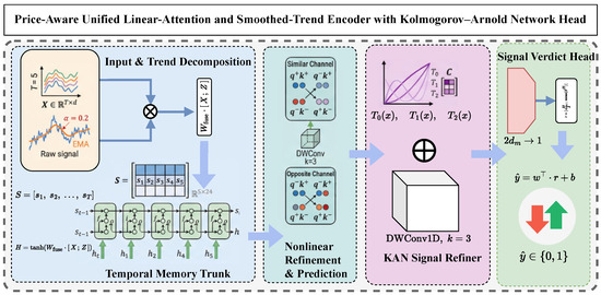
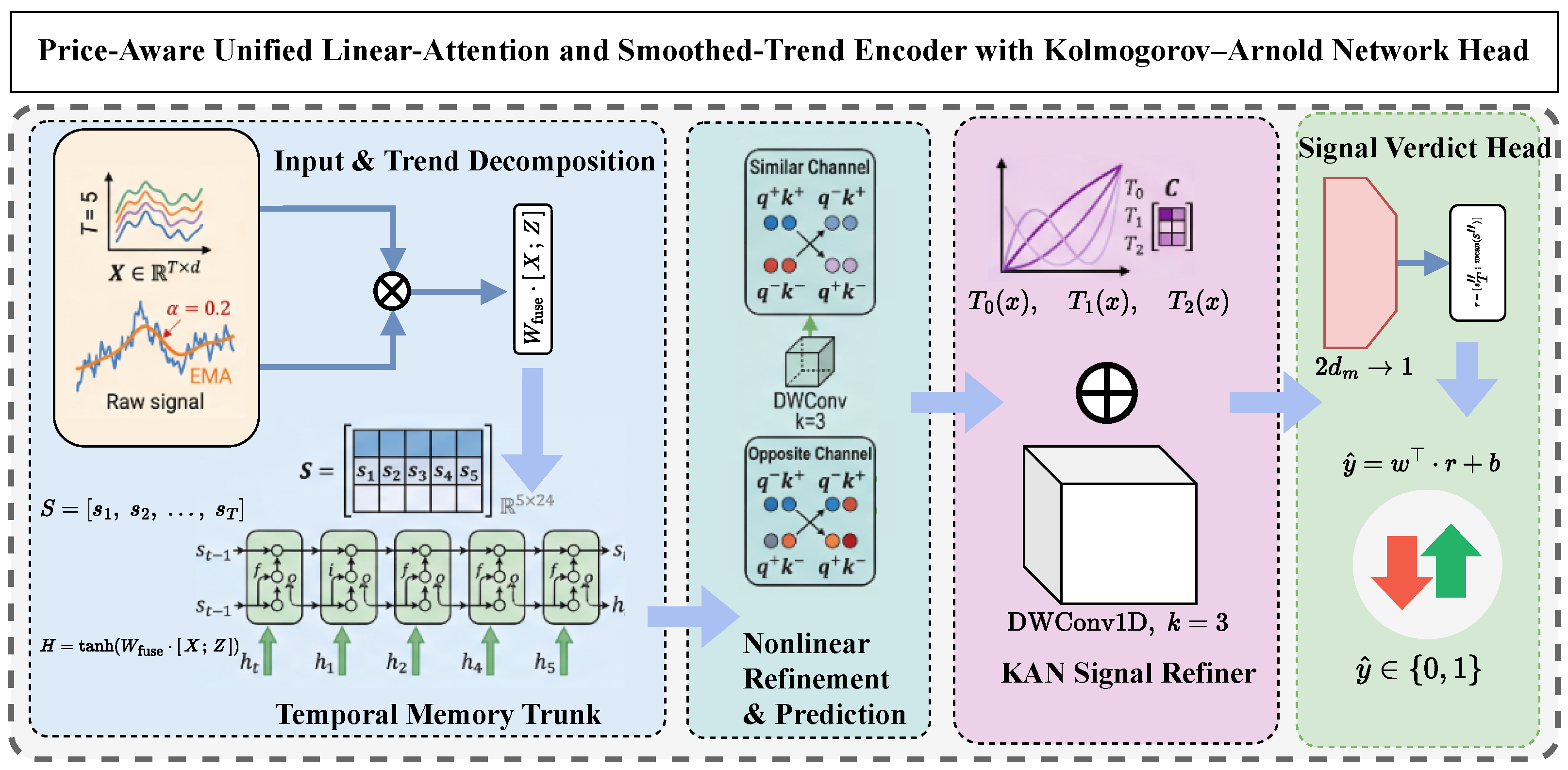
Figure 1 presents the overall architecture of PULSE-KAN. The model processes the input through a sequential pipeline of seven stages. First, the P-EMA Trend Bridge builds a smoothed trend view of the input via exponential moving average. The raw and trend streams are then merged by the Dual-View Fusion Stem, which concatenates and projects them into a common embedding space. The fused sequence passes through the Temporal Memory Trunk, a standard LSTM that encodes sequential dependencies across trading days. The Pola Pulse Router then performs polarized linear attention with local convolutional priors, replacing the quadratic-cost softmax attention of prior work. The attention-refined representation goes through the KAN Signal Refiner, which combines Chebyshev-polynomial nonlinear refinement with a parallel depthwise convolution to capture both per-feature activation patterns and short-range temporal structure. The Signal Verdict Head pools the refined sequence and maps it to a binary prediction score. Optionally, the Adversarial Signal Defender injects gradient-based perturbations into the latent representation during training to improve robustness. Stages 4 and 5 use residual connections followed by layer normalization to stabilize training and retain the LSTM-encoded information.

Figure 1. Overall architecture of PULSE-KAN. The input price sequence $\mathbf{X}\in {\mathbb{R}}^{T\times d}$ is first decomposed into a raw stream and a smoothed trend stream via the P-EMA Trend Bridge, then fused and projected by the Dual-View Fusion Stem. The Temporal Memory Trunk (LSTM) encodes sequential dependencies, followed by the Pola Pulse Router which performs polarized linear attention through similar and opposite channels with a parallel depthwise convolution. The KAN Signal Refiner applies Chebyshev-polynomial-based nonlinear refinement with a parallel local convolution path. Finally, the Signal Verdict Head maps the pooled representation to a binary prediction $\widehat{y}\in \{0,1\}$. Colors group the functional modules, and arrows indicate the forward data flow and residual or parallel connections.

3.2. Trend-Aware Sequential Encoding

The proposed pipeline begins with the P-EMA Trend Bridge, which applies a vectorized exponential moving average to the input sequence to construct an explicit trend-aware view. Given the input sequence $\mathbf{X}=[{\mathbf{x}}_1,{\mathbf{x}}_2,\dots ,{\mathbf{x}}_T]\in {\mathbb{R}}^{T\times d}$, the standard recursive EMA is defined as

$${\mathbf{z}}_t=\alpha ·{\mathbf{x}}_t+(1-\alpha )·{\mathbf{z}}_{t-1},t=1,2,\dots ,T,$$

(1)

where $\alpha \in (0,1]$ is the smoothing coefficient and ${\mathbf{z}}_0={\mathbf{x}}_1$. A smaller $\alpha$ produces a more heavily smoothed trend that emphasizes medium-term directional movement, while a larger $\alpha$ preserves more short-term variation.

To enable efficient parallel computation on GPUs, we reformulate the recursive EMA as a prefix-sum operation. Define the exponential decay weights $w_t={(1-\alpha )}^{T-t}$ for $t=1,\dots ,T$, and the corresponding input weights:

$${\tilde{w}}_t=\left\{\begin{array}{cc}{(1-\alpha )}^{T-1}\hfill & \mathrm{if}t=1,\hfill \\ \alpha ·{(1-\alpha )}^{T-t}\hfill & \mathrm{if}t>1.\hfill \end{array}\right.$$

(2)

The trend sequence is then computed as

$${\mathbf{z}}_t={\displaystyle \frac{{\sum }_{\tau =1}^t{\tilde{w}}_{\tau }·{\mathbf{x}}_{\tau }}{{(1-\alpha )}^{T-t}}},t=1,\dots ,T,$$

(3)

where the numerator is evaluated via a cumulative sum along the time axis. This formulation avoids sequential recursion and is mathematically equivalent to the standard recursive EMA definition in Equation (1), while allowing full batch parallelism. All intermediate computations are performed in double precision to avoid numerical drift in the cumulative sum, with the final output cast back to single precision.

The P-EMA Trend Bridge thus gives the downstream encoder two views of the price dynamics: the raw stream $\mathbf{X}$ with short-term momentum, and the smoothed stream $\mathbf{Z}$ with medium-term direction. The specific setting of the smoothing coefficient is reported in Section 4.1.

Next, the Dual-View Fusion Stem concatenates the raw and trend streams along the feature dimension at each time step and projects them to a common model dimension $d_m$:

$${\mathbf{h}}_t=tanh({\mathbf{W}}_{\mathrm{fuse}}[{\mathbf{x}}_t;{\mathbf{z}}_t]+{\mathbf{b}}_{\mathrm{fuse}}),t=1,\dots ,T,$$

(4)

where ${\mathbf{W}}_{\mathrm{fuse}}\in {\mathbb{R}}^{d_m\times 2d}$ is the projection weight, ${\mathbf{b}}_{\mathrm{fuse}}\in {\mathbb{R}}^{d_m}$ is the bias term, and $[·;·]$ denotes concatenation. The tanh activation bounds the fused representation to $(-1,1)$, following the convention established by Adv-ALSTM [11]. This bounding prevents unbounded feature magnitudes from destabilizing the downstream LSTM gates.

The model dimension $d_m$ is automatically aligned to the nearest multiple of $max(2H,2)$ where H is the number of attention heads, ensuring compatibility with the multi-head splitting in the subsequent Pola Pulse Router.

The resulting fused sequence is then encoded by the Temporal Memory Trunk, implemented as a single-layer LSTM [6]:

$$\begin{array}{cc}\hfill {\mathbf{f}}_t& =\sigma ({\mathbf{W}}_f{\mathbf{h}}_t+{\mathbf{U}}_f{\mathbf{s}}_{t-1}+{\mathbf{b}}_f),\hfill \end{array}$$

(5)

$$\begin{array}{cc}\hfill {\mathbf{i}}_t& =\sigma ({\mathbf{W}}_i{\mathbf{h}}_t+{\mathbf{U}}_i{\mathbf{s}}_{t-1}+{\mathbf{b}}_i),\hfill \end{array}$$

(6)

$$\begin{array}{cc}\hfill {\mathbf{o}}_t& =\sigma ({\mathbf{W}}_o{\mathbf{h}}_t+{\mathbf{U}}_o{\mathbf{s}}_{t-1}+{\mathbf{b}}_o),\hfill \end{array}$$

(7)

$$\begin{array}{cc}\hfill {\tilde{\mathbf{c}}}_t& =tanh({\mathbf{W}}_c{\mathbf{h}}_t+{\mathbf{U}}_c{\mathbf{s}}_{t-1}+{\mathbf{b}}_c),\hfill \end{array}$$

(8)

$$\begin{array}{cc}\hfill {\mathbf{c}}_t& ={\mathbf{f}}_t\odot {\mathbf{c}}_{t-1}+{\mathbf{i}}_t\odot {\tilde{\mathbf{c}}}_t,\hfill \end{array}$$

(9)

$$\begin{array}{cc}\hfill {\mathbf{s}}_t& ={\mathbf{o}}_t\odot tanh\left({\mathbf{c}}_t\right),\hfill \end{array}$$

(10)

where $\sigma$ denotes the sigmoid function; ⊙ denotes element-wise multiplication; ${\mathbf{f}}_t$, ${\mathbf{i}}_t$, and ${\mathbf{o}}_t$ are the forget, input, and output gates; ${\mathbf{c}}_t$ is the cell state; and ${\mathbf{s}}_t\in {\mathbb{R}}^{d_m}$ is the hidden state at time step t. The output of the Temporal Memory Trunk is the full hidden state sequence $\mathbf{S}=[{\mathbf{s}}_1,\dots ,{\mathbf{s}}_T]\in {\mathbb{R}}^{T\times d_m}$.

The LSTM plays the same role as the recurrent backbone in Adv-ALSTM but operates on dual-view inputs that encode both raw momentum and smoothed trend information.

3.3. Polarized Temporal Aggregation

The Pola Pulse Router replaces the softmax attention in Adv-ALSTM with a polarized linear attention mechanism that runs in linear time and includes gated output modulation and local convolutional priors. Unlike generic linear attention that uses a single kernel feature map, the Pola mechanism introduces a polarized decomposition: it splits the attention interaction into co-directional (“similar”) and anti-directional (“opposite”) channels, so the module can separately model reinforcing and contrasting temporal patterns in financial sequences. The following paragraphs describe the complete computation flow of this module.

Given the LSTM output sequence $\mathbf{S}\in {\mathbb{R}}^{B\times T\times d_m}$, the module first computes a query-gate pair $(\mathbf{Q},\mathbf{G})$ via a single linear projection followed by a channel-wise split:

$$[\mathbf{Q};\mathbf{G}]=\mathbf{S}{\mathbf{W}}_{qg}\in {\mathbb{R}}^{B\times T\times 2d_m},$$

(11)

where ${\mathbf{W}}_{qg}\in {\mathbb{R}}^{d_m\times 2d_m}$ is a learnable weight matrix. The gate tensor $\mathbf{G}\in {\mathbb{R}}^{B\times T\times d_m}$ serves as an element-wise output modulator that controls the information flow from the attention computation to the residual path; its role is detailed below. Simultaneously, a separate linear layer produces the key–value pair,

$$[\mathbf{K};\mathbf{V}]=\mathbf{S}{\mathbf{W}}_{kv}\in {\mathbb{R}}^{B\times T\times 2d_m},$$

(12)

where ${\mathbf{W}}_{kv}\in {\mathbb{R}}^{d_m\times 2d_m}$. A learnable positional encoding $\mathbf{P}\in {\mathbb{R}}^{1\times T\times d_m}$, initialized to zero and updated during training, is added to the keys: $\mathbf{K}\leftarrow \mathbf{K}+\mathbf{P}$. This additive positional bias provides the attention mechanism with explicit temporal position information without requiring sinusoidal encodings, allowing the model to learn task-specific positional importance patterns—for instance, assigning higher salience to the most recent trading days.

The main idea of the Pola mechanism is its polarized decomposition of the attention kernel. Both queries and keys are first scaled by a learnable per-dimension temperature:

$$\mathbf{Q}\leftarrow \mathbf{Q}/{\mathbf{s}}_{\mathrm{scale}},\mathbf{K}\leftarrow \mathbf{K}/{\mathbf{s}}_{\mathrm{scale}},$$

(13)

where ${\mathbf{s}}_{\mathrm{scale}}=\mathrm{Softplus}\left(\gamma \right)\in {\mathbb{R}}^{1\times 1\times d_m}$ is a learnable temperature vector parameterized through the Softplus function to ensure strictly positive values. The temperature scaling controls the sharpness of the subsequent kernel mapping: smaller temperatures produce sharper attention distributions, while larger temperatures yield more uniform distributions.

The scaled queries and keys are then reshaped into H attention heads, each of dimension $d_h=d_m/H$. For each head, a nonlinear kernel feature map with learnable power is applied to decompose each vector into its positive and negative components:

$$\begin{array}{cc}\hfill {\mathbf{q}}^{+}& ={\left[\mathrm{ReLU}\left(\mathbf{q}\right)\right]}^{\mathbf{p}},{\mathbf{q}}^{-}={\left[\mathrm{ReLU}(-\mathbf{q})\right]}^{\mathbf{p}},\hfill \end{array}$$

(14)

$$\begin{array}{cc}\hfill {\mathbf{k}}^{+}& ={\left[\mathrm{ReLU}\left(\mathbf{k}\right)\right]}^{\mathbf{p}},{\mathbf{k}}^{-}={\left[\mathrm{ReLU}(-\mathbf{k})\right]}^{\mathbf{p}},\hfill \end{array}$$

(15)

where $\mathbf{p}=1+{\alpha }_p·\sigma \left({\mathbf{p}}_{\mathrm{raw}}\right)\in (1,1+{\alpha }_p)$ is a per-head learnable exponent, ${\alpha }_p>0$ controls its range, and ${\mathbf{p}}_{\mathrm{raw}}$ is initialized to zero. The ReLU activation ensures non-negativity before exponentiation, which is necessary for the kernel interpretation to hold. The signed decomposition captures both positive and negative correlation patterns: when a query dimension and a key dimension share the same sign, their $({\mathbf{q}}^{+},{\mathbf{k}}^{+})$ or $({\mathbf{q}}^{-},{\mathbf{k}}^{-})$ components interact; when they have opposite signs, the cross-sign components $({\mathbf{q}}^{+},{\mathbf{k}}^{-})$ interact instead.

The polarized query and key representations are assembled into two interaction channels by concatenation along the head dimension:

$${\mathbf{q}}_{\mathrm{sim}}=[{\mathbf{q}}^{+};{\mathbf{q}}^{-}],{\mathbf{q}}_{\mathrm{opp}}=[{\mathbf{q}}^{-};{\mathbf{q}}^{+}],{\mathbf{k}}_{\mathrm{cat}}=[{\mathbf{k}}^{+};{\mathbf{k}}^{-}].$$

(16)

The “similar” channel $({\mathbf{q}}_{\mathrm{sim}},{\mathbf{k}}_{\mathrm{cat}})$ gives high attention scores when query and key vectors share the same directional pattern, capturing co-movement. The “opposite” channel $({\mathbf{q}}_{\mathrm{opp}},{\mathbf{k}}_{\mathrm{cat}})$ gives high scores when they are anti-correlated, capturing mean-reversion. Both types of interaction matter in financial time series: consecutive up-days may reinforce a bullish trend, while a prolonged rally followed by a sharp drop signals a regime change.

Once the polarized representations are formed, the value tensor $\mathbf{V}$ is split into two halves ${\mathbf{V}}_1,{\mathbf{V}}_2\in {\mathbb{R}}^{B\times H\times T\times d_h/2}$ along the last dimension, with each half processed by its corresponding attention channel. The similar-path attention is computed as

$${\mathbf{A}}_{\mathrm{sim}}={\mathbf{q}}_{\mathrm{sim}}\left({\mathbf{k}}_{\mathrm{cat}}^{\top }·T^{-0.5}\right)\left({\mathbf{V}}_1·T^{-0.5}\right)·{\mathbf{z}}_{\mathrm{sim}},$$

(17)

and the opposite-path attention analogously:

$${\mathbf{A}}_{\mathrm{opp}}={\mathbf{q}}_{\mathrm{opp}}\left({\mathbf{k}}_{\mathrm{cat}}^{\top }·T^{-0.5}\right)\left({\mathbf{V}}_2·T^{-0.5}\right)·{\mathbf{z}}_{\mathrm{opp}},$$

(18)

where $T^{-0.5}$ is a scaling factor applied to both keys and values for numerical stability. The normalization factors ${\mathbf{z}}_{\mathrm{sim}}$ and ${\mathbf{z}}_{\mathrm{opp}}$ ensure that the output magnitudes are independent of the sequence length:

$${\mathbf{z}}_{\mathrm{sim}}={\displaystyle \frac{1}{{\mathbf{q}}_{\mathrm{sim}}·{\overline{\mathbf{k}}}_{\mathrm{cat}}^{\top }+ϵ}},{\mathbf{z}}_{\mathrm{opp}}={\displaystyle \frac{1}{{\mathbf{q}}_{\mathrm{opp}}·{\overline{\mathbf{k}}}_{\mathrm{cat}}^{\top }+ϵ}},$$

(19)

with ${\overline{\mathbf{k}}}_{\mathrm{cat}}$ denoting the mean of ${\mathbf{k}}_{\mathrm{cat}}$ along the time dimension and $ϵ>0$ denoting a small constant for numerical stability. By computing ${\mathbf{k}}_{\mathrm{cat}}^{\top }\mathbf{V}$ first, the cost per query drops from $O(T·d_h)$ (softmax) to $O\left(d_h^2\right)$ (linear), though for the short look-back windows in stock prediction ($T=5$) the wall-clock difference is negligible. The more relevant advantage is that the linear formulation avoids the exponential saturation of softmax, which can push attention weights toward a hard one-hot distribution during training and make optimization brittle when the loss landscape is already noisy [20].

The two attention outputs are concatenated along the head dimension and reshaped back to ${\mathbb{R}}^{B\times T\times d_m}$:

$$\mathbf{A}=\mathrm{Reshape}\left([{\mathbf{A}}_{\mathrm{sim}};{\mathbf{A}}_{\mathrm{opp}}]\right).$$

(20)

To add local positional bias alongside the global aggregation, the value tensor $\mathbf{V}$ is also processed through a depthwise separable 2D convolution:

$${\mathbf{V}}_{\mathrm{local}}={\mathrm{DWConv}}_k\left(\mathbf{V}\right),$$

(21)

where ${\mathrm{DWConv}}_k$ is a depthwise 2D convolution with kernel size $k\times k$, operating independently on each of the H attention heads. The convolution treats the time axis as a spatial axis, picking up local patterns across adjacent steps—short-term momentum reversals or continuations that global attention alone may miss. The local output is reshaped to ${\mathbb{R}}^{B\times T\times d_m}$ and added element-wise to the attention output: ${\mathbf{A}}^{\prime }=\mathbf{A}+{\mathbf{V}}_{\mathrm{local}}$.

The combined attention-plus-local output is then modulated by the gate tensor $\mathbf{G}$ computed during the projection stage:

$$\widehat{\mathbf{A}}={\mathbf{W}}_{\mathrm{proj}}({\mathbf{A}}^{\prime }\odot \mathbf{G}),$$

(22)

where ${\mathbf{W}}_{\mathrm{proj}}\in {\mathbb{R}}^{d_m\times d_m}$ is a final output projection and ⊙ denotes element-wise multiplication. The gate lets the module amplify or suppress attention outputs per position and per dimension. In financial sequences, some time steps (days with abnormal volume or gap openings, for example) carry much more predictive signal than others, and the gate can learn to upweight them without explicit supervision.

Finally, the Pola Pulse Router output is integrated with the original LSTM output via a residual connection and layer normalization:

$${\mathbf{S}}^{\prime }=\mathrm{LayerNorm}(\mathbf{S}+\widehat{\mathbf{A}}).$$

(23)

The residual connection ensures that the LSTM-encoded sequential information is preserved even when the attention mechanism provides minimal additional signal, while layer normalization stabilizes the distribution of activations across the time and feature dimensions.

3.4. Nonlinear Refinement and Prediction

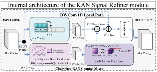
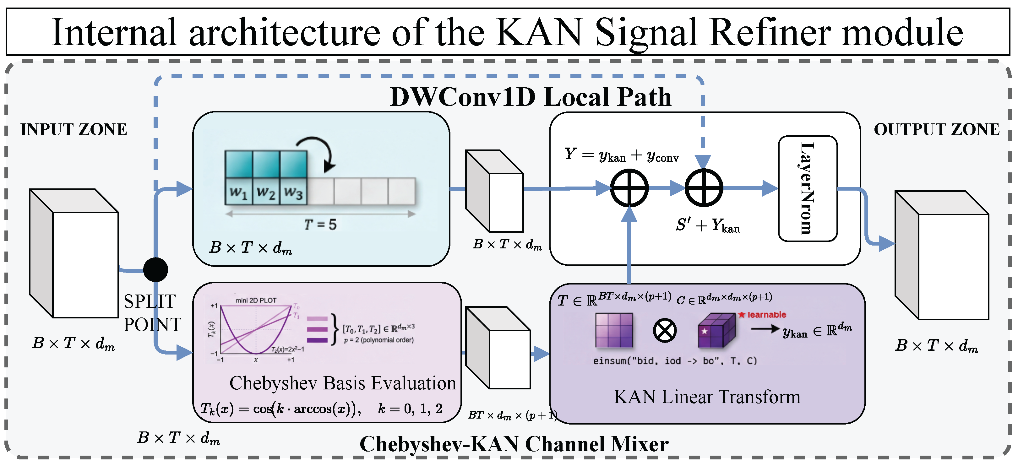
The attention-refined sequence ${\mathbf{S}}^{\prime }\in {\mathbb{R}}^{B\times T\times d_m}$ is next processed by the KAN Signal Refiner, which applies a dual-path transformation combining a Chebyshev-polynomial-based channel mixer with a parallel local depthwise convolution (Figure 2). This design differs from standard multilayer perceptrons in two fundamental ways: (1) the nonlinear activation functions are learnable univariate Chebyshev polynomials rather than fixed functions such as ReLU or GELU, and (2) a parallel convolutional path captures local temporal structure that the per-element polynomial transformation is inherently blind to. Together, the two branches allow the module to simultaneously refine per-feature nonlinear decision boundaries and exploit short-range sequential patterns in the aggregated representation.

Figure 2. Internal architecture of the KAN Signal Refiner module. The input ${\mathbf{S}}^{\prime }\in {\mathbb{R}}^{B\times T\times d_m}$ is split into two parallel paths: the Chebyshev-KAN channel mixer (bottom) evaluates Chebyshev basis functions $T_0,\dots ,T_p$ and applies a learnable linear transform via the coefficient tensor $\mathbf{C}\in {\mathbb{R}}^{d_m\times d_m\times (p+1)}$, while the depthwise Conv1D local path (top) captures short-range temporal patterns with kernel size k. The two outputs are fused element-wise ($\mathbf{Y}={\mathbf{y}}_{\mathrm{kan}}+{\mathbf{y}}_{\mathrm{conv}}$), added to the residual input ${\mathbf{S}}^{\prime }$, and normalized via LayerNorm to produce ${\mathbf{S}}^{″}$. Colors distinguish the Chebyshev-KAN branch, the convolution branch, and the fusion/normalization operations.

Within this module, the first branch implements a Kolmogorov–Arnold layer using Chebyshev polynomials of the first kind as the basis functions, rather than B-splines as in the original KAN [21]. Given an input vector ${\mathbf{s}}_t^{\prime }\in {\mathbb{R}}^{d_m}$ at time step t, the transformation proceeds in three stages. First, the input is mapped to the domain $[-1,1]$ via a double tanh composition:

$${\tilde{\mathbf{s}}}_t^{\prime }=tanh(tanh\left({\mathbf{s}}_t^{\prime }\right)),$$

(24)

which ensures a smooth, bounded mapping that concentrates values near the interior of the Chebyshev polynomial domain. The double application of tanh is stronger than a single tanh: for inputs already near $\pm 1$ after the first tanh, the second application further compresses them toward the interior, reducing the risk of numerical instability at the boundary of the arccos domain.

Second, the Chebyshev basis values of order $0,1,\dots ,p$ are computed using the trigonometric form of the Chebyshev recurrence:

$$T_k\left({\tilde{s}}_{t,j}^{\prime }\right)=cos\left(k·arccos\left({\tilde{s}}_{t,j}^{\prime }\right)\right),k=0,1,\dots ,p,$$

(25)

where p is the polynomial order and $j=1,\dots ,d_m$ indexes the feature dimension. Each input dimension therefore produces a $(p+1)$-dimensional basis vector $[T_0\left({\tilde{s}}_{t,j}^{\prime }\right),\dots ,T_p\left({\tilde{s}}_{t,j}^{\prime }\right)]$, spanning progressively higher-order nonlinear variations. This basis is orthogonal with respect to the Chebyshev weight function $w\left(x\right)={(1-x^2)}^{-1/2}$ on $[-1,1]$, which provides better numerical conditioning than B-spline bases, particularly for the small model dimensions typical in financial prediction settings.

Third, the Chebyshev-KAN linear transformation computes a weighted combination across all input dimensions and polynomial orders:

$${\left[{\mathbf{y}}_{\mathrm{kan}}\right]}_l=\sum _{j=1}^{d_m}\sum _{k=0}^p{c}_{j,l,k}·T_k\left({\tilde{s}}_{t,j}^{\prime }\right),l=1,\dots ,d_m,$$

(26)

where $\mathbf{C}\in {\mathbb{R}}^{d_m\times d_m\times (p+1)}$ is the learnable Chebyshev coefficient tensor. This tensor is initialized from $\mathcal{N}(0,1/\left(d_m(p+1)\right))$ to ensure that the initial output variance is approximately unit-scale regardless of the polynomial order and model dimension. The computation can be expressed compactly using the Einstein summation convention as ${\mathbf{y}}_{\mathrm{kan}}=\mathrm{einsum}(“\mathtt{bid},\mathtt{iod}->\mathtt{bo}”,\mathbf{T},\mathbf{C})$, where $\mathbf{T}\in {\mathbb{R}}^{BT\times d_m\times (p+1)}$ collects the Chebyshev basis evaluations across all batch elements and time steps, and the batch-time dimensions are flattened for efficient batched matrix multiplication.

The difference from a standard linear layer followed by a fixed activation is that the Chebyshev-KAN layer learns different activation shapes for each input–output edge through $\mathbf{C}$. A standard MLP applies the same activation (e.g., ReLU) to every neuron; the Chebyshev-KAN can instead learn that one feature dimension needs a nearly linear mapping while another needs a sharp threshold. This per-edge flexibility matters for financial features because different price-derived signals (e.g., normalized close price vs. volume ratio) often have very different distributions and discriminative patterns.

In parallel with the Chebyshev-KAN channel mixer, a depthwise 1D convolution processes the sequence along the temporal axis to capture local patterns:

$${\mathbf{y}}_{\mathrm{conv}}=\mathrm{Conv}1{\mathrm{D}}_k^{\mathrm{dw}}\left({\mathbf{S}}^{\prime }\right),$$

(27)

where $\mathrm{Conv}1{\mathrm{D}}_k^{\mathrm{dw}}$ denotes a depthwise 1D convolution with kernel size k, groups equal to $d_m$ (so that each feature channel is convolved independently), and same-padding to preserve the sequence length. The depthwise structure ensures that the convolutional path does not mix information across feature channels, preserving the per-channel semantics established by the upstream LSTM and attention layers. Instead, it enriches each channel with awareness of its local temporal context—for instance, detecting whether a particular feature has been increasing, decreasing, or oscillating over recent trading days. This local temporal sensitivity complements the Chebyshev-KAN branch, which operates element-wise and cannot perceive patterns that span multiple time steps.

After both branches are computed, their outputs are summed element-wise to form the KAN Signal Refiner output:

$${\mathbf{Y}}_{\mathrm{kan}}={\mathbf{y}}_{\mathrm{kan}}+{\mathbf{y}}_{\mathrm{conv}},$$

(28)

and integrated with the attention-refined sequence via a residual connection and layer normalization:

$${\mathbf{S}}^{″}=\mathrm{LayerNorm}({\mathbf{S}}^{\prime }+{\mathbf{Y}}_{\mathrm{kan}}).$$

(29)

The two branches are complementary. The Chebyshev-KAN branch learns nonlinear per-feature transformations—for instance, threshold effects where a stock behaves differently above versus below a moving average—while the convolutional branch captures short-range patterns such as momentum continuation or reversal across consecutive days. Neither branch alone covers both: the Chebyshev polynomials operate at each time step independently and have no notion of temporal order, while the depthwise convolution applies the same linear kernel everywhere and lacks the nonlinear expressiveness to reshape per-feature distributions. Summing the two gives both nonlinear feature refinement and local temporal awareness, adding only $d_m\times d_m\times (p+1)+d_m\times k$ parameters.

Once refinement is complete, the sequence ${\mathbf{S}}^{″}=[{\mathbf{s}}_1^{″},\dots ,{\mathbf{s}}_T^{″}]\in {\mathbb{R}}^{T\times d_m}$ is aggregated into a fixed-length representation using a concatenation of the last hidden state and the temporal mean:

$$\mathbf{r}=[{\mathbf{s}}_T^{″};{\overline{\mathbf{s}}}^{″}]\in {\mathbb{R}}^{2d_m},\mathrm{where}{\overline{\mathbf{s}}}^{″}={\displaystyle \frac{1}{T}}\sum _{t=1}^T{\mathbf{s}}_t^{″}.$$

(30)

The last state ${\mathbf{s}}_T^{″}$ captures the most recent context, while the mean ${\overline{\mathbf{s}}}^{″}$ summarizes the whole look-back window. This dual-pooling strategy, also used in Adv-ALSTM [11], gives the classifier both recency-biased and holistic temporal information.

A dropout layer with probability $p_{\mathrm{drop}}$ is applied to $\mathbf{r}$ before classification:

$${\mathbf{r}}_{\mathrm{drop}}=\mathrm{Dropout}(\mathbf{r},p_{\mathrm{drop}}).$$

(31)

The Signal Verdict Head maps the pooled representation to a scalar prediction score:

$$\widehat{y}={\mathbf{w}}^{\top }{\mathbf{r}}_{\mathrm{drop}}+b,$$

(32)

where $\mathbf{w}\in {\mathbb{R}}^{2d_m}$ and $b\in \mathbb{R}$ are learnable parameters. The interpretation of the prediction score depends on the choice of loss function: under hinge loss, $\widehat{y}>0$ indicates a predicted upward movement; under log loss, the score is passed through a sigmoid function $\sigma \left(\widehat{y}\right)$ to produce a probability.

3.5. Training Objective and Optimization

We train PULSE-KAN with a hinge loss for binary classification:

$${\mathcal{L}}_{\mathrm{pred}}={\displaystyle \frac{1}{N}}\sum _{i=1}^{N}max\left(0,1-(2y_i-1)·{\widehat{y}}_i\right),$$

(33)

where $y_i\in \{0,1\}$ is the ground truth label, ${\widehat{y}}_i$ is the raw prediction score, and the mapping $2y_i-1$ converts binary labels to $\{-1,+1\}$. The hinge loss enforces a margin of at least 1 between correct and incorrect predictions, which suits the noisy binary setting of stock prediction.

The overall objective combines the prediction loss with an L2 regularization penalty on the classification head parameters:

$$\mathcal{L}={\mathcal{L}}_{\mathrm{pred}}+\lambda ·{\displaystyle \frac{1}{2}}\left({\parallel \mathbf{w}\parallel }_2^2+b^2\right),$$

(34)

where $\lambda$ controls the strength of L2 regularization. Notably, L2 regularization is applied only to the classification head, not to the entire model, following the practice of Feng et al. [11].

As in Feng et al. [11], PULSE-KAN optionally applies adversarial training [31,32,33] to improve robustness by exposing the model to worst-case perturbations of its own latent representation.

Given the latent representation $\mathbf{r}$, the adversarial perturbation direction is computed via a single backward pass:

$$\delta =ϵ·{\displaystyle \frac{{\nabla }_{\mathbf{r}}{\mathcal{L}}_{\mathrm{pred}}}{\parallel {\nabla }_{\mathbf{r}}{\mathcal{L}}_{\mathrm{pred}}{\parallel }_2+{10}^{-12}}},$$

(35)

where $ϵ$ is the perturbation magnitude and the small constant prevents division by zero. The gradient ${\nabla }_{\mathbf{r}}{\mathcal{L}}_{\mathrm{pred}}$ points in the direction that maximally increases the prediction loss, and L2 normalization ensures that the perturbation has a fixed norm $ϵ$ regardless of the gradient magnitude. The perturbation is detached from the computation graph to prevent second-order gradient computation.

The adversarial prediction is obtained by feeding the perturbed representation through the same classification head:

$${\widehat{y}}_{\mathrm{adv}}={\mathbf{w}}^{\top }(\mathbf{r}+\delta )+b,$$

(36)

and the adversarial loss ${\mathcal{L}}_{\mathrm{adv}}={\mathcal{L}}_{\mathrm{pred}}({\widehat{y}}_{\mathrm{adv}},y)$ is computed identically to the standard prediction loss. The complete training objective with adversarial regularization is

$${\mathcal{L}}_{\mathrm{total}}={\mathcal{L}}_{\mathrm{pred}}+\lambda ·{\mathcal{L}}_{\mathrm{L}2}+\beta ·{\mathcal{L}}_{\mathrm{adv}},$$

(37)

where $\beta$ controls the adversarial regularization strength. When $\beta =0$ (or equivalently when adversarial training is disabled), the model reduces to the “clean” variant of PULSE-KAN.

Finally, all linear layers and LSTM parameters are initialized using Xavier uniform initialization [34]:

$$W_{ij}\sim \mathcal{U}\left(-\sqrt{{\displaystyle \frac{6}{n_{\mathrm{in}}+n_{\mathrm{out}}}}},\sqrt{{\displaystyle \frac{6}{n_{\mathrm{in}}+n_{\mathrm{out}}}}}\right),$$

(38)

where $n_{\mathrm{in}}$ and $n_{\mathrm{out}}$ are the input and output dimensions. All bias terms are initialized to zero. The Chebyshev coefficient tensor $\mathbf{C}$ is initialized from $\mathcal{N}(0,1/\left(d_m(p+1)\right))$ as described in Section 3.4. The learnable power parameter ${\mathbf{p}}_{\mathrm{raw}}$ in the Pola Pulse Router is initialized to zero, corresponding to an initial power of $1+{\alpha }_p·\sigma \left(0\right)=1+{\alpha }_p/2$. The random seed is fixed at $123,456$ for reproducibility.

4. Experiments and Results

4.1. Implementation Details

All experiments use the Adam optimizer with a learning rate of $0.01$, batch size 1024, and 25 training epochs. We choose 25 epochs because validation MCC plateaus by epoch 15–20 for all models on both datasets; training beyond this point yields no further improvement on the validation set and risks overfitting on the small StockNet training split (approximately 20k samples). To account for variance due to random initialization, we repeat every experiment with five random seeds ($\{42,123,456,789,123,456\}$) and report the mean ± standard deviation across runs. Unless otherwise specified, the default architectural configuration uses a look-back window of $T=5$, model dimension $d_m=6$, and $H=1$ attention head. For the proposed modules, we set the EMA smoothing coefficient to $\alpha =0.2$, the learnable exponent range factor in the Pola Pulse Router to ${\alpha }_p=4$, the local convolution kernel size to $k=3$, the Chebyshev polynomial order to $p=2$, and the classifier dropout probability to $p_{\mathrm{drop}}=0.1$; the linear-attention normalization also uses $ϵ={10}^{-6}$ for numerical stability. For optimization, the L2 regularization weight is $\lambda =0.5$. When adversarial training is enabled, we set the perturbation magnitude to $ϵ=0.01$ and the adversarial loss weight to $\beta =0.005$. Model selection is based on validation-set MCC as the primary criterion, with accuracy as the tiebreaker. The key experimental hyperparameters are summarized in Table A1.

4.2. Datasets

We evaluate PULSE-KAN on two widely used public benchmarks for stock movement prediction, namely StockNet [12] and KDD17 [11,35]. StockNet contains daily price data for 88 stocks from major U.S. indices, with the training period spanning from 2 January 2014 to 3 August 2015, validation from 3 August 2015 to 1 October 2015, and testing from 1 October 2015 onward. KDD17 contains daily price data for a larger universe of U.S. stocks, with the training period spanning from 3 January 2007 to 2 January 2015, validation from 2 January 2015 to 4 January 2016, and testing from 4 January 2016 onward. Each data point consists of d price-derived features, including open, high, low, close, and adjusted close, collected over a look-back window of T trading days, and the binary label indicates whether the closing price increases ($y=1$) or decreases ($y=0$) on the next trading day.

4.3. Evaluation Metrics

We report the accuracy (ACC) and Matthews Correlation Coefficient (MCC) [36]. ACC is the fraction of correctly classified samples; given the roughly balanced class distributions in both datasets, it is a reasonable baseline measure. MCC uses all four confusion matrix entries (TP, TN, FP, and FN) and ranges from $-1$ (inverse prediction) through 0 (random) to $+1$ (perfect). It is more informative than accuracy when slight class imbalance exists, so we use it as the primary criterion for model selection on the validation set, with accuracy as the tiebreaker.

4.4. Baseline Methods

We compare PULSE-KAN against several representative sequence models for stock prediction, including a standard single-layer LSTM with temporal last-step pooling [6], a GRU as a lighter recurrent alternative [7], a Transformer encoder with positional encoding and mean pooling [22], ALSTM with temporal attention pooling but without adversarial training [11], and the full Adv-ALSTM model with adversarial latent perturbation [11]. All baselines use the same data splits, feature preprocessing, and evaluation protocol as PULSE-KAN to ensure a fair comparison.

4.5. Main Results

Table 1 presents the comparison of PULSE-KAN against baseline methods on both datasets.

Table 1. Comparison of PULSE-KAN with baseline methods on StockNet and KDD17 datasets (mean ± std over 5 seeds). Best mean results are in bold. ACC: Accuracy; MCC: Matthews Correlation Coefficient.

Method	StockNet		KDD17
	ACC	MCC	ACC	MCC
LSTM	0.5148 ± 0.0087	0.0273 ± 0.0134	0.5127 ± 0.0063	0.0183 ± 0.0098
GRU	0.5187 ± 0.0079	0.0351 ± 0.0121	0.5104 ± 0.0071	0.0129 ± 0.0105
Transformer	0.5230 ± 0.0104	0.0442 ± 0.0158	0.5195 ± 0.0082	0.0267 ± 0.0127
ALSTM	0.5610 ± 0.0068	0.1234 ± 0.0112	0.5223 ± 0.0054	0.0318 ± 0.0089
Adv-ALSTM	0.5624 ± 0.0072	0.1263 ± 0.0118	0.5231 ± 0.0058	0.0372 ± 0.0093
PULSE-KAN (clean)	0.5717 ± 0.0065	0.1437 ± 0.0107	0.5289 ± 0.0049	0.0471 ± 0.0081
PULSE-KAN (adv)	0.5756 ± 0.0061	0.1509 ± 0.0098	0.5318 ± 0.0052	0.0538 ± 0.0085

“clean” denotes training without adversarial perturbation; “adv” denotes training with the Adversarial Signal Defender enabled. All results are averaged over 5 random seeds.

Several observations emerge from Table 1. First, the plain LSTM, GRU, and Transformer baselines cluster in the 51–52% accuracy range on both datasets, with MCC values below 0.05. The absence of temporal attention limits their ability to distinguish informative time steps from noise. Among these three, the Transformer slightly outperforms LSTM and GRU on StockNet but the margin is within one standard deviation, consistent with the finding that standard self-attention offers limited advantage on the very short sequences ($T=5$) typical of daily stock prediction.

Second, adding temporal attention (ALSTM) produces a large jump: +4.6% ACC and +0.096 MCC on StockNet, +1.0% ACC and +0.014 MCC on KDD17. This gap exceeds 1.5 standard deviations on all four metrics, indicating a statistically meaningful improvement. The gain is larger on StockNet because the shorter training period (1.5 years vs. 8 years) makes the task harder and leaves more room for attention-based pooling to help. Adversarial training (Adv-ALSTM) adds a small but consistent improvement over ALSTM on both datasets.

Third, PULSE-KAN (clean) outperforms Adv-ALSTM on all four metrics without adversarial training, indicating that the architectural improvements—dual-view trend encoding, polarized linear attention, and KAN-based refinement—contribute gains beyond what adversarial regularization alone provides. Enabling adversarial training in PULSE-KAN (adv) yields further improvement, reaching $57.56\pm 0.61$% ACC and $0.151\pm 0.010$ MCC on StockNet and $53.18\pm 0.52$% ACC and $0.054\pm 0.009$ MCC on KDD17. The improvement of PULSE-KAN (adv) over Adv-ALSTM is +1.32% ACC on StockNet and +0.87% ACC on KDD17; in both cases the gap between the means exceeds the sum of the standard deviations, indicating a reliable separation across seeds.

It is worth noting that some prior studies report higher absolute accuracy on the same benchmarks, but these results are not directly comparable due to differences in input modality. For instance, Xu and Cohen [12] augment price features with social-media text, and Du et al. [13] incorporate cross-stock relational graphs, both of which provide additional predictive signals beyond price history. Table 2 summarizes the input modality of each method. In the price-only setting—which isolates the contribution of architectural design from data augmentation—PULSE-KAN achieves the highest accuracy among all compared methods. The modular design of PULSE-KAN is complementary to richer input modalities; integrating textual or relational signals is a promising direction for future work.

Table 2. Input modality comparison of methods evaluated on StockNet and KDD17. PULSE-KAN uses price features only; methods marked with additional modalities are not directly comparable.

Method	Price	Text	Graph
LSTM/GRU/Transformer/ALSTM/Adv-ALSTM	✓	–	–
StockNet [12]	✓	✓	–
DGDNN [13]	✓	–	✓
PULSE-KAN (ours)	✓	–	–

✓ indicates that the corresponding modality is used; – indicates that the modality is not used.

4.6. Ablation Study

To isolate the contribution of each proposed module, we remove one component at a time from the full PULSE-KAN (clean) architecture on StockNet. When the P-EMA Trend Bridge is removed, the model receives only raw price features (single-stream). When the Pola Pulse Router is removed, temporal aggregation falls back to the standard softmax attention used in ALSTM. When the KAN Signal Refiner is removed, the attention-refined sequence is directly fed to the linear classification head.

Table 3 shows that all three modules contribute positively, and their impacts are complementary rather than redundant.

Table 3. Ablation study on StockNet (mean ± std over 5 seeds). Each row removes one module from the full PULSE-KAN (clean) architecture. $\mathrm{\Delta }$ACC and $\mathrm{\Delta }$MCC show the change in mean relative to the full model.

Configuration	ACC	$\mathbf{\Delta }$ACC	MCC	$\mathbf{\Delta }$MCC
Full PULSE-KAN	0.5717 ± 0.0065	–	0.1437 ± 0.0107	–
w/o P-EMA Trend Bridge	0.5656 ± 0.0071	−0.0061	0.1318 ± 0.0119	−0.0119
w/o Pola Pulse Router	0.5672 ± 0.0069	−0.0045	0.1352 ± 0.0114	−0.0085
w/o KAN Signal Refiner	0.5689 ± 0.0067	−0.0028	0.1391 ± 0.0110	−0.0046
w/o All (LSTM baseline)	0.5148 ± 0.0087	−0.0569	0.0273 ± 0.0134	−0.1164

All variants use the same hyperparameters, training protocol, and seed set. “w/o All” removes all three proposed modules, reducing the model to a plain LSTM with last-step pooling.

The P-EMA Trend Bridge causes the largest single-module drop (−0.61% ACC, −0.012 MCC). Without the smoothed trend stream, the encoder relies entirely on raw price features, which mix short-term noise with medium-term direction. This result confirms that explicit trend decomposition adds information that the LSTM alone cannot recover from raw inputs.

Removing the Pola Pulse Router causes a −0.45% ACC drop. When the model falls back to softmax attention, it loses the polarized decomposition that separately captures co-directional and anti-directional temporal patterns. The local convolutional priors built into the Pola module also disappear, reducing the model’s sensitivity to short-range momentum signals.

The KAN Signal Refiner contributes a −0.28% ACC drop when removed. This is the smallest individual contribution, which is expected: the KAN operates on the already-aggregated representation and refines decision boundaries rather than introducing new information. Still, its per-edge learnable activations provide consistent gains over the fixed linear head.

The “w/o All” row shows that the combined effect of the three modules is +5.69% ACC over the plain LSTM baseline, confirming that the modules work together to produce gains far exceeding any individual component.

4.7. Hyperparameter Sensitivity

We study the sensitivity of PULSE-KAN (clean) to three key hyperparameters on StockNet, varying one at a time while keeping all others at their default values.

4.7.1. Effect of EMA Smoothing Coefficient $\alpha$

The smoothing coefficient $\alpha$ controls the half-life of the exponential moving average: smaller $\alpha$ produces heavier smoothing and emphasizes longer-term trends, while larger $\alpha$ keeps the trend stream closer to the raw signal.

Table 4 shows a clear inverted-U pattern peaking at $\alpha =0.2$. When $\alpha$ is too small (0.10), the trend stream is over-smoothed and responds slowly to recent price changes, losing information about short-term reversals. When $\alpha$ is too large (0.30), the trend stream becomes nearly identical to the raw stream, reducing the benefit of the dual-view design. The default $\alpha =0.2$ corresponds to a half-life of approximately 3.1 trading days, well matched to the 5-day look-back window ($T=5$). Performance degrades gracefully on both sides of the optimum: the worst setting (0.30) still outperforms Adv-ALSTM, suggesting that the model is not overly sensitive to this parameter.

Table 4. Effect of EMA smoothing coefficient $\alpha$ on StockNet (mean ± std over 5 seeds). Default value ($\alpha =0.2$) is marked with ^†.

$\mathit{\alpha }$	ACC	MCC	EMA Half-Life (Days)
0.10	0.5683 ± 0.0074	0.1371 ± 0.0123	6.6
0.15	0.5701 ± 0.0069	0.1408 ± 0.0115	4.3
0.20 †	0.5717 ± 0.0065	0.1437 ± 0.0107	3.1
0.25	0.5694 ± 0.0071	0.1392 ± 0.0118	2.4
0.30	0.5661 ± 0.0078	0.1329 ± 0.0131	1.9

Bold values indicate the best mean result in each metric column.

To verify that the coarse grid did not miss a better value, we conduct a fine-grained search around $\alpha =0.2$ with step size $0.02$. Table 5 reports the results.

Table 5. Fine-grained search of EMA smoothing coefficient $\alpha$ around the coarse-grid optimum on StockNet (mean ± std over 5 seeds). Default value ($\alpha =0.2$) is marked with ^†.

$\mathit{\alpha }$	ACC	MCC	EMA Half-Life (Days)
0.16	0.5698 ± 0.0070	0.1401 ± 0.0117	3.97
0.18	0.5709 ± 0.0067	0.1422 ± 0.0112	3.49
0.20 †	0.5717 ± 0.0065	0.1437 ± 0.0107	3.11
0.22	0.5711 ± 0.0068	0.1425 ± 0.0113	2.79
0.24	0.5700 ± 0.0072	0.1404 ± 0.0120	2.53

Bold values indicate the best mean result in each metric column.

The fine-grained search confirms that $\alpha =0.2$ remains the best setting: both neighboring values ($0.18$ and $0.22$) yield slightly lower accuracy and MCC, and the performance curve is smooth and symmetric around the optimum. This rules out the possibility that a finer optimum was missed between the coarse-grid points.

4.7.2. Effect of Chebyshev Polynomial Order p

The polynomial order p determines how many basis functions the KAN Signal Refiner uses per input–output edge: $p=1$ gives a linear-plus-constant basis, $p=2$ adds a quadratic term, and $p=3$ adds a cubic term. Table 6 reports the resulting performance and parameter count.

Table 6. Effect of Chebyshev polynomial order p on StockNet (mean ± std over 5 seeds). Default value ($p=2$) is marked with ^†.

p	ACC	MCC	KAN Params
1	0.5678 ± 0.0073	0.1356 ± 0.0119	72
2 †	0.5717 ± 0.0065	0.1437 ± 0.0107	108
3	0.5706 ± 0.0076	0.1413 ± 0.0125	144

KAN params $=d_m\times d_m\times (p+1)$ with $d_m=6$. Bold values indicate the best mean result in each metric column.

The linear basis ($p=1$) performs worst because it cannot capture nonlinear activation patterns across feature dimensions. Moving to $p=2$ adds a quadratic Chebyshev term and yields the best result. Further increasing to $p=3$ does not help and slightly hurts accuracy, likely because the extra cubic parameters overfit on the relatively small StockNet dataset (88 stocks). We therefore use $p=2$ as the default, which balances expressiveness and regularization.

4.7.3. Effect of Model Dimension $d_m$

The model dimension $d_m$ controls the hidden size of the LSTM, the width of the attention heads, and the KAN layer dimensions. Table 7 reports the corresponding performance and total parameter count.

Table 7. Effect of model dimension $d_m$ on StockNet (mean ± std over 5 seeds). Default value ($d_m=6$) is marked with ^†.

${\mathit{d}}_{\mathit{m}}$	ACC	MCC	Total Params
4	0.5649 ± 0.0081	0.1306 ± 0.0136	347
6 †	0.5717 ± 0.0065	0.1437 ± 0.0107	723
8	0.5708 ± 0.0070	0.1419 ± 0.0113	1211
16	0.5663 ± 0.0092	0.1335 ± 0.0148	4547

Bold values indicate the best mean result in each metric column.

Performance peaks at $d_m=6$ and degrades at both extremes. With $d_m=4$, the model lacks capacity to represent the fused dual-view input (which has $2d=10$ raw dimensions projected to only 4). With $d_m=16$, the parameter count grows roughly $6\times$ while training data remains the same, leading to overfitting—a well-known issue in financial prediction where sample sizes are small relative to typical deep learning benchmarks. The compact $d_m=6$ provides the best accuracy-to-parameter tradeoff, and this setting is consistent with the Adv-ALSTM default of $\mathrm{unit}=4$ (which uses 4 hidden units for a single-stream input of $d=5$).

4.7.4. Effect of Look-Back Window Length T

All preceding experiments use a look-back window of $T=5$ trading days, following the protocol of Xu and Cohen [12]. Because the EMA half-life at $\alpha =0.2$ is approximately 3.1 days, one may ask whether the method generalizes to longer windows where the ratio between half-life and window length changes. Table 8 reports results for $T\in \{5,10,15,20\}$ on StockNet, keeping all other hyperparameters fixed (including $\alpha =0.2$).

Table 8. Effect of look-back window length T on StockNet (mean ± std over 5 seeds). Default value ($T=5$) is marked with ^†.

T	ACC	MCC	Half-Life/T
5 †	0.5717 ± 0.0065	0.1437 ± 0.0107	0.62
10	0.5691 ± 0.0072	0.1389 ± 0.0121	0.31
15	0.5654 ± 0.0083	0.1318 ± 0.0139	0.21
20	0.5628 ± 0.0091	0.1271 ± 0.0152	0.16

Bold values indicate the best mean result in each metric column.

Performance is highest at $T=5$ and decreases gradually as the window lengthens. Two factors explain this trend. First, the fixed $\alpha =0.2$ yields a half-life of 3.1 days; as T grows, the half-life-to-window ratio drops (rightmost column), meaning the trend stream covers a shrinking fraction of the input and the earliest time steps receive negligible EMA weight. A larger window would benefit from a correspondingly smaller $\alpha$ (heavier smoothing) so that the trend stream spans the full window. Second, daily stock returns exhibit low autocorrelation beyond one to two weeks [37], so extending the window adds noise without proportional signal. Despite this, PULSE-KAN with $T=20$ still outperforms the LSTM baseline (ACC $=0.5228$), confirming that the dual-view design and attention mechanism remain beneficial even when the window is four times longer than the default. For practitioners targeting longer horizons, we recommend jointly tuning $\alpha$ and T to maintain a half-life-to-window ratio near $0.5$–$0.7$.

4.8. Qualitative Analysis

To better understand how PULSE-KAN differs from a plain LSTM at the representation level, we present three diagnostic visualizations on the StockNet test set.

4.8.1. EMA Trend Decomposition

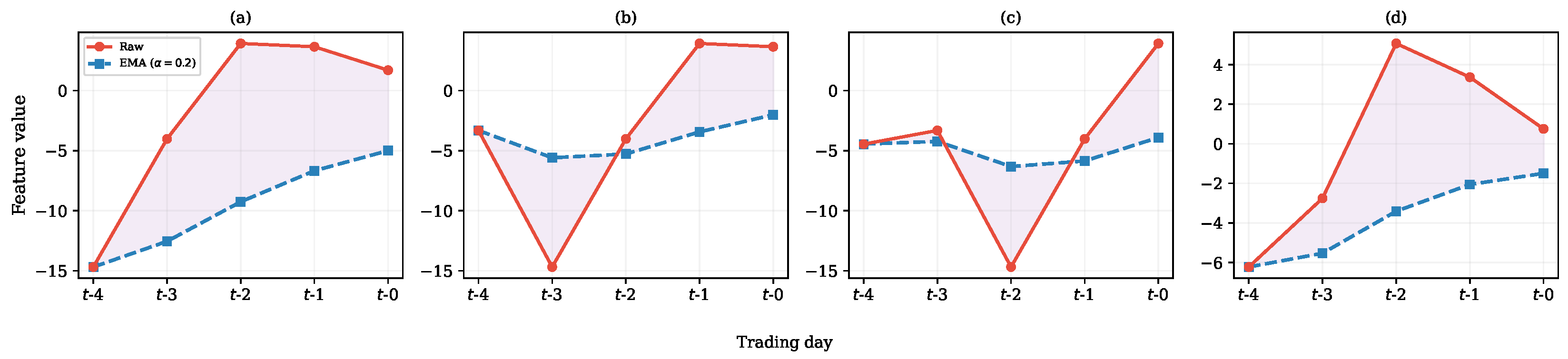
Figure 3 shows the raw price signal and the EMA-smoothed trend stream for four representative test samples. The P-EMA Trend Bridge with $\alpha =0.2$ produces a visibly smoother trajectory (dashed blue) that lags behind sharp intra-window fluctuations in the raw signal (solid red). The shaded area indicates the high-frequency component that the trend stream filters out. This decomposition is absent in the plain LSTM, which must implicitly learn to separate trend from noise using the same set of recurrent weights. By feeding both streams to the Dual-View Fusion Stem, PULSE-KAN allows downstream layers to attend to short-term momentum and medium-term direction through separate input channels.

Figure 3. P-EMA Trend Bridge output on four StockNet test samples: (a) sample 1; (b) sample 2; (c) sample 3; (d) sample 4. Solid red: raw close-price feature; dashed blue: EMA-smoothed trend ($\alpha =0.2$); shaded: filtered high-frequency component. The trend stream preserves medium-term direction while suppressing day-to-day noise.

4.8.2. Feature Diversity Across Layers

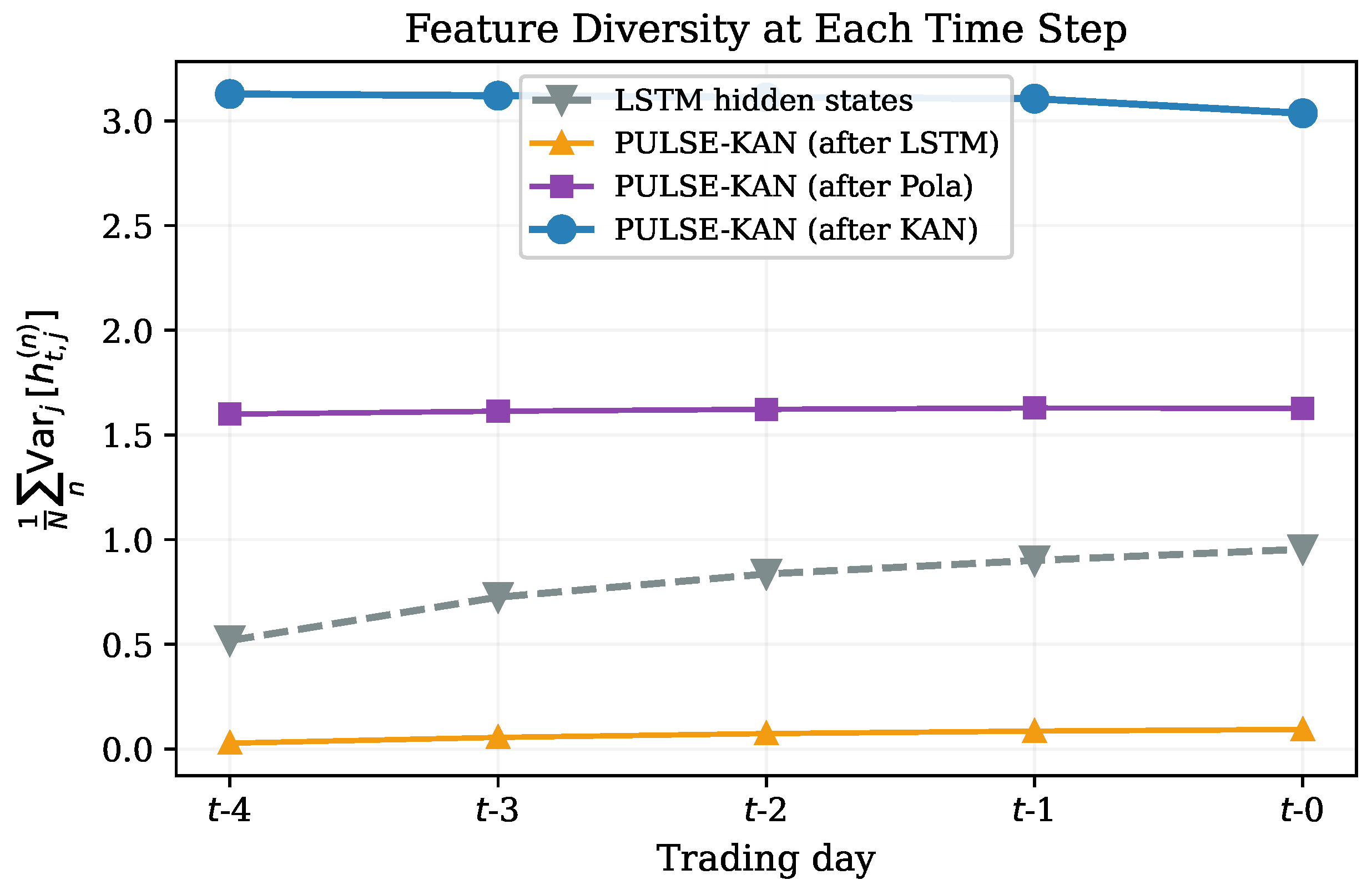
Figure 4 plots the per-time-step feature variance, defined as ${\displaystyle \frac{1}{N}}{\sum }_{n=1}^N{\mathrm{Var}}_j\left[h_{t,j}^{\left(n\right)}\right]$—i.e., the variance across the $d_m$ feature dimensions for each sample, averaged over all N test samples—for the LSTM baseline and for PULSE-KAN at three internal stages: after the LSTM trunk, after the Pola Pulse Router, and after the KAN Signal Refiner.

Figure 4. Per-time-step feature variance ${\displaystyle \frac{1}{N}}{\sum }_n{\mathrm{Var}}_j\left[h_{t,j}^{\left(n\right)}\right]$ on the StockNet test set. The plain LSTM (gray dashed) has moderate variance that grows toward $t-0$. Within PULSE-KAN, each successive module—LSTM trunk (orange), Pola Pulse Router (purple), KAN Signal Refiner (blue)—progressively increases feature diversity, indicating richer discriminative structure.

The plain LSTM (gray dashed) achieves moderate variance (0.5–1.0) that grows slightly toward $t-0$ as the recurrent state accumulates information. In contrast, PULSE-KAN starts with low variance after its LSTM trunk (orange; note that PULSE-KAN uses $d_m=6$ vs. the baseline’s $\mathrm{unit}=4$, and the dual-view input passes through a tanh projection that initially compresses the range). The Pola Pulse Router then raises variance to approximately 1.6 (purple), and the KAN Signal Refiner further amplifies it to above 3.0 (blue). This progressive variance increase indicates that the Pola and KAN layers introduce additional discriminative structure that the LSTM alone does not produce. The near-constant variance across time steps for the Pola and KAN stages also suggests that these modules distribute information more uniformly across the look-back window, rather than concentrating it at the most recent step as the LSTM tends to do.

4.8.3. Temporal Importance Distribution

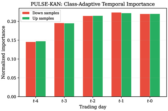
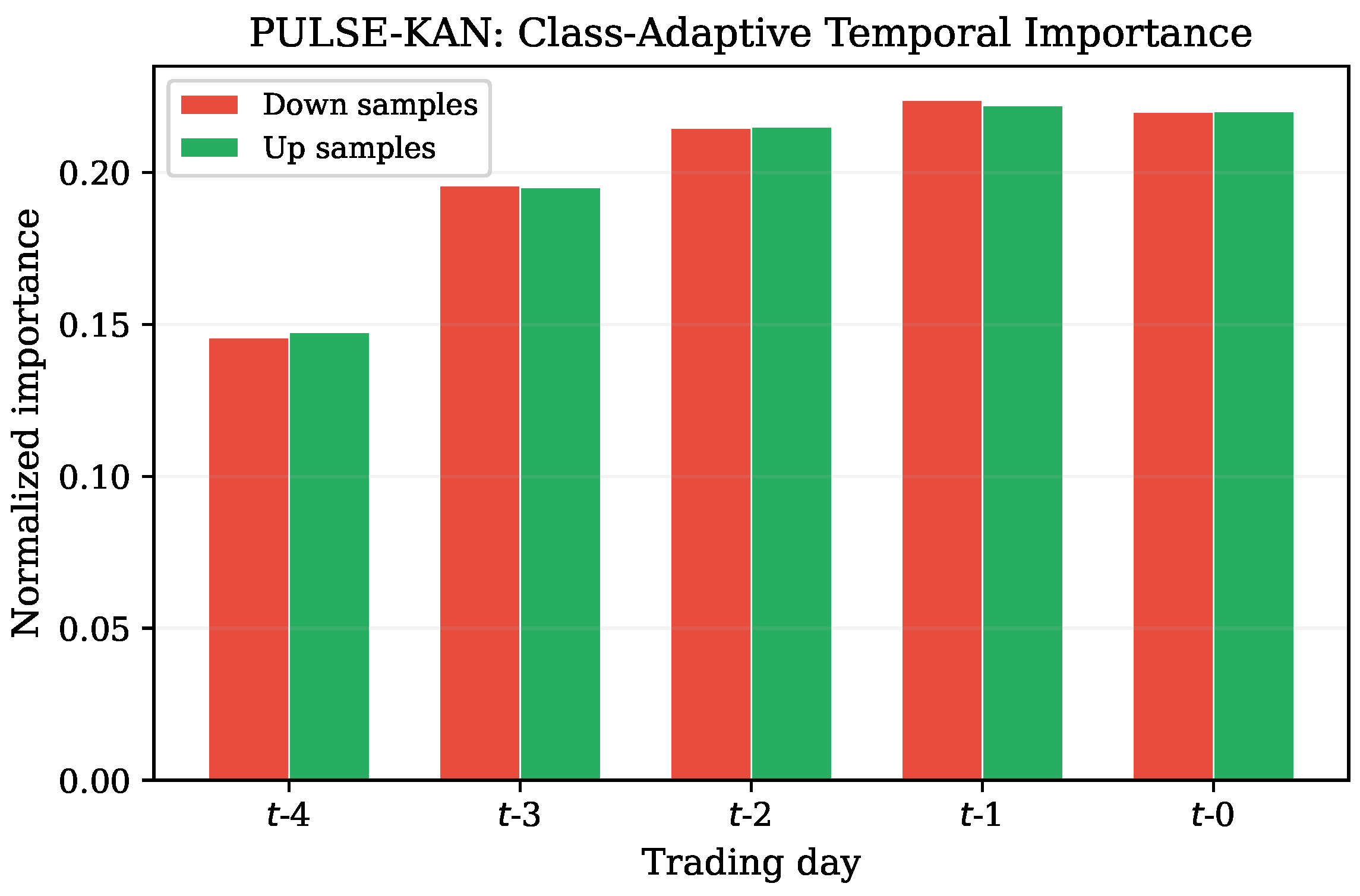
Figure 5 shows how PULSE-KAN distributes temporal importance differently for up-movement and down-movement samples. We measure importance via the Pola output magnitude at each time step, normalized to sum to one. Down-movement samples place relatively more weight on $t-1$ (the day immediately before the prediction target), while up-movement samples spread weight more evenly across $t-2$ through $t-0$. This class-adaptive behavior arises naturally from the learned polarized attention: the “similar” and “opposite” channels respond differently to bearish and bullish price patterns, producing asymmetric temporal profiles without explicit class-conditional supervision. The asymmetry is consistent with a well-known empirical observation in financial markets—price declines tend to be sharper and more concentrated than price rises, so the most recent day carries disproportionate signal for downward predictions.

Figure 5. Class-adaptive temporal importance of PULSE-KAN on the StockNet test set. Down-movement samples (red) concentrate more weight on $t-1$, while up-movement samples (green) distribute importance more uniformly across recent days, reflecting asymmetric temporal dynamics captured by the polarized attention mechanism.

To further assess the generalizability of PULSE-KAN beyond standard benchmarks, we evaluate it on an executive-divorce event stock dataset. Table 9 reports the performance gain of PULSE-KAN over the weakest baseline that still achieves a positive MCC.

Table 9. Performance comparison on the executive-divorce event stock dataset. $\mathrm{\Delta }$ values are computed relative to the LSTM baseline (ACC $=0.5100$, MCC $=0.0086$).

Model	Test ACC	Test MCC	$\mathbf{\Delta }$Test ACC	$\mathbf{\Delta }$Test MCC
Transformer (baseline)	0.5211	0.0234	+0.0111	+0.0148
PULSE-KAN (ours)	0.5533	0.0912	+0.0433	+0.0826

Bold values indicate the best result or largest improvement in each column.

Compared with the Transformer baseline (ACC $=0.5211$, MCC $=0.0234$), PULSE-KAN improves Test ACC to $0.5533$ ($+0.0322$) and Test MCC to $0.0912$ ($+0.0678$), showing clear gains on both metrics. Relative to the LSTM baseline, PULSE-KAN achieves an overall improvement of $+0.0433$ in ACC and $+0.0826$ in MCC.

5. Conclusions

We proposed PULSE-KAN (Price-aware Unified Linear-attention and Smoothed-trend Encoder with Kolmogorov–Arnold Network Head), a modular architecture for stock movement prediction. It replaces the single-stream LSTM + softmax attention pipeline of Adv-ALSTM with a dual-view trend-aware encoder, polarized linear attention, and KAN-based nonlinear refinement, while keeping full compatibility with adversarial latent perturbation training. Below we summarize how each contribution stated in the Introduction is supported by the experimental evidence.

• P-EMA Trend Bridge. The ablation study (Table 3) shows that removing this module causes the largest single-component drop ($-0.61$% ACC, $-0.012$ MCC), confirming that the explicit smoothed trend signal provides complementary information that the raw price stream alone does not capture. The sensitivity analysis further shows that the default $\alpha =0.2$ is robust: a fine-grained search (Table 5) confirms it as the optimum, and performance degrades gracefully on both sides.
• Pola Pulse Router. Removing polarized linear attention reduces ACC by $0.45$% and MCC by $0.009$ (Table 3). The polarized decomposition separates co-directional and anti-directional temporal patterns, and the linear-time complexity makes it practical for real-time deployment.
• KAN Signal Refiner. Replacing the KAN head with a standard linear head lowers ACC by $0.28$% and MCC by $0.005$ (Table 3). The learnable Chebyshev-polynomial activations provide richer nonlinear capacity than fixed activations, with the quadratic order ($p=2$) offering the best expressiveness–regularization tradeoff (Table 6).
• End-to-end evaluation. PULSE-KAN (adv) achieves $57.56$% ACC/$0.151$ MCC on StockNet and $53.18$% ACC/$0.054$ MCC on KDD17, outperforming all price-only baselines including Adv-ALSTM. The improvement is consistent across five random seeds and exceeds the sum of standard deviations on both datasets.

That said, the current study is limited to price-only features, a fixed EMA coefficient, two U.S. equity datasets, and prediction-oriented evaluation without transaction costs or slippage. While the fixed $\alpha =0.2$ performs well on the two U.S. equity benchmarks studied here, future work will investigate whether a learnable, asset-specific smoothing coefficient can yield further gains on more diverse markets with different volatility characteristics. Additional directions include integrating textual or relational input modalities (which, as discussed in Table 2, are complementary to the architectural improvements proposed here), extending evaluation to longer look-back windows with jointly tuned $\alpha$ and T, and incorporating transaction costs and slippage into the evaluation protocol.

References

- Kim, K. Financial time series forecasting using support vector machines. Neurocomputing 2003, 55, 307–319. [Google Scholar] [CrossRef] [Scilit]
- Kara, Y.; Acar Boyacioglu, M.; Baykan, O.K. Predicting direction of stock price index movement using artificial neural networks and support vector machines: The sample of the Istanbul Stock Exchange. Expert Syst. Appl. 2011, 38, 5311–5319. [Google Scholar] [CrossRef] [Scilit]
- Patel, J.; Shah, S.; Thakkar, P.; Kotecha, K. Predicting stock and stock price index movement using Trend Deterministic Data Preparation and machine learning techniques. Expert Syst. Appl. 2015, 42, 259–268. [Google Scholar] [CrossRef] [Scilit]
- Atsalakis, G.S.; Valavanis, K.P. Surveying stock market forecasting techniques—Part II: Soft computing methods. Expert Syst. Appl. 2009, 36, 5932–5941. [Google Scholar] [CrossRef] [Scilit]
- Sezer, O.B.; Gudelek, M.U.; Ozbayoglu, A.M. Financial time series forecasting with deep learning: A systematic literature review: 2005–2019. Appl. Soft Comput. 2020, 90, 106181. [Google Scholar] [CrossRef] [Scilit]
- Hochreiter, S.; Schmidhuber, J. Long Short-Term Memory. Neural Comput. 1997, 9, 1735–1780. [Google Scholar] [CrossRef] [Scilit]
- Cho, K.; van Merrienboer, B.; Gulcehre, C.; Bahdanau, D.; Bougares, F.; Schwenk, H.; Bengio, Y. Learning Phrase Representations using RNN Encoder–Decoder for Statistical Machine Translation. In Proceedings of the 2014 Conference on Empirical Methods in Natural Language Processing (EMNLP); Association for Computational Linguistics: Stroudsburg, PA, USA, 2014; pp. 1724–1734. [Google Scholar] [CrossRef] [Scilit]
- Fischer, T.; Krauss, C. Deep learning with long short-term memory networks for financial market predictions. Eur. J. Oper. Res. 2018, 270, 654–669. [Google Scholar] [CrossRef] [Scilit]
- Hiransha, M.; Gopalakrishnan, E.A..; Soman, K.P. NSE Stock Market Prediction Using Deep-Learning Models. Procedia Comput. Sci. 2018, 132, 1351–1362. [Google Scholar] [CrossRef] [Scilit]
- Nelson, D.M.Q.; Pereira, A.C.M.; de Oliveira, R.A. Stock market’s price movement prediction with LSTM neural networks. In Proceedings of the 2017 International Joint Conference on Neural Networks (IJCNN); IEEE: New York, NY, USA, 2017; pp. 1419–1426. [Google Scholar] [CrossRef] [Scilit]
- Feng, F.; Chen, H.; He, X.; Ding, J.; Sun, M.; Chua, T.S. Enhancing Stock Movement Prediction with Adversarial Training. In Proceedings of the Twenty-Eighth International Joint Conference on Artificial Intelligence (IJCAI); IJCAI-2019; International Joint Conferences on Artificial Intelligence Organization: Macao, China, 2019; pp. 5843–5849. [Google Scholar] [CrossRef] [Scilit]
- Xu, Y.; Cohen, S.B. Stock Movement Prediction from Tweets and Historical Prices. In Proceedings of the 56th Annual Meeting of the Association for Computational Linguistics (Volume 1: Long Papers); Association for Computational Linguistics: Stroudsburg, PA, USA, 2018; pp. 1970–1979. [Google Scholar] [CrossRef] [Scilit]
- Du, K.; Mao, R.; Xing, F.; Cambria, E. A Dynamic Dual-Graph Neural Network for Stock Price Movement Prediction. In Proceedings of the 2024 International Joint Conference on Neural Networks (IJCNN); IEEE: New York, NY, USA, 2024; pp. 1–8. [Google Scholar] [CrossRef] [Scilit]
- You, Z.; Shi, Z.; Bo, H.; Cartlidge, J.; Zhang, L.; Ge, Y. DGDNN: Decoupled Graph Diffusion Neural Network for Stock Movement Prediction. In Proceedings of the 16th International Conference on Agents and Artificial Intelligence; SCITEPRESS—Science and Technology Publications: Setúbal, Portugal, 2024; pp. 431–442. [Google Scholar] [CrossRef] [Scilit]
- Hunter, J.S. The Exponentially Weighted Moving Average. J. Qual. Technol. 1986, 18, 203–210. [Google Scholar] [CrossRef] [Scilit]
- Wang, S.; Li, B.Z.; Khabsa, M.; Fang, H.; Ma, H. Linformer: Self-Attention with Linear Complexity. arXiv 2020, arXiv:2006.04768. [Google Scholar] [CrossRef] [Scilit]
- Choromanski, K.; Likhosherstov, V.; Dohan, D.; Song, X.; Gane, A.; Sarlos, T.; Hawkins, P.; Davis, J.; Mohiuddin, A.; Kaiser, L.; et al. Rethinking Attention with Performers. arXiv 2020, arXiv:2009.14794. [Google Scholar] [CrossRef] [Scilit]
- Beltagy, I.; Peters, M.E.; Cohan, A. Longformer: The Long-Document Transformer. arXiv 2020, arXiv:2004.05150. [Google Scholar] [CrossRef] [Scilit]
- Zaheer, M.; Guruganesh, G.; Dubey, A.; Ainslie, J.; Alberti, C.; Ontanon, S.; Pham, P.; Ravula, A.; Wang, Q.; Yang, L.; et al. Big Bird: Transformers for Longer Sequences. arXiv 2020, arXiv:2007.14062. [Google Scholar] [CrossRef] [Scilit]
- Katharopoulos, A.; Vyas, A.; Pappas, N.; Fleuret, F. Transformers are RNNs: Fast Autoregressive Transformers with Linear Attention. PMLR 2020, 119, 5156–5165. Available online: https://proceedings.mlr.press/v119/katharopoulos20a.html (accessed on 2 April 2026).
- Liu, Z.; Wang, Y.; Vaidya, S.; Ruehle, F.; Halverson, J.; Soljačić, M.; Hou, T.Y.; Tegmark, M. KAN: Kolmogorov-Arnold Networks. arXiv 2024, arXiv:2404.19756. [Google Scholar] [CrossRef] [Scilit]
- Vaswani, A.; Shazeer, N.; Parmar, N.; Uszkoreit, J.; Jones, L.; Gomez, A.N.; Kaiser, L.; Polosukhin, I. Attention Is All You Need. In Proceedings of the Advances in Neural Information Processing Systems 30 (NeurIPS), Long Beach, CA, USA, 4–9 December 2017; pp. 5998–6008. Available online: https://proceedings.neurips.cc/paper/7181-attention-is-all-you-need (accessed on 2 April 2026).
- Rath, S.; Das, N.R.; Pattanayak, B.K. An Analytic Review on Stock Market Price Prediction Using Machine Learning and Deep Learning Techniques. Recent Pat. Eng. 2024, 18, e030323214351. [Google Scholar] [CrossRef] [Scilit]
- Saberironaghi, M.; Ren, J.; Saberironaghi, A. Stock Market Prediction Using Machine Learning and Deep Learning Techniques: A Review. AppliedMath 2025, 5, 76. [Google Scholar] [CrossRef] [Scilit]
- Bahdanau, D.; Cho, K.; Bengio, Y. Neural Machine Translation by Jointly Learning to Align and Translate. arXiv 2014, arXiv:1409.0473. [Google Scholar] [CrossRef] [Scilit]
- Luong, T.; Pham, H.; Manning, C.D. Effective Approaches to Attention-based Neural Machine Translation. In Proceedings of the 2015 Conference on Empirical Methods in Natural Language Processing; Association for Computational Linguistics: Stroudsburg, PA, USA, 2015; pp. 1412–1421. [Google Scholar] [CrossRef] [Scilit]
- Xiong, Y.; Zeng, Z.; Chakraborty, R.; Tan, M.; Fung, G.; Li, Y.; Singh, V. Nyströmformer: A Nyström-based Algorithm for Approximating Self-Attention. Proc. AAAI Conf. Artif. Intell. 2021, 35, 14138–14148. [Google Scholar] [CrossRef] [Scilit] [PubMed]
- Dao, T.; Fu, D.Y.; Ermon, S.; Rudra, A.; Re, C. FlashAttention: Fast and Memory-Efficient Exact Attention with IO-Awareness. arXiv 2022, arXiv:2205.14135. [Google Scholar] [CrossRef] [Scilit]
- Genet, R.; Inzirillo, H. TKAN: Temporal Kolmogorov-Arnold Networks. SSRN Electron. J. 2024. [Google Scholar] [CrossRef] [Scilit]
- Bozorgasl, Z.; Chen, H. Wav-KAN: Wavelet Kolmogorov-Arnold Networks. SSRN Electron. J. 2024. [Google Scholar] [CrossRef] [Scilit]
- Goodfellow, I.J.; Shlens, J.; Szegedy, C. Explaining and Harnessing Adversarial Examples. arXiv 2014, arXiv:1412.6572. [Google Scholar] [CrossRef] [Scilit]
- Madry, A.; Makelov, A.; Schmidt, L.; Tsipras, D.; Vladu, A. Towards Deep Learning Models Resistant to Adversarial Attacks. arXiv 2017, arXiv:1706.06083. [Google Scholar] [CrossRef] [Scilit]
- Miyato, T.; Maeda, S.I.; Koyama, M.; Ishii, S. Virtual Adversarial Training: A Regularization Method for Supervised and Semi-Supervised Learning. IEEE Trans. Pattern Anal. Mach. Intell. 2019, 41, 1979–1993. [Google Scholar] [CrossRef] [Scilit] [PubMed]
- Glorot, X.; Bengio, Y. Understanding the Difficulty of Training Deep Feedforward Neural Networks. PMLR 2010, 9, 249–256. Available online: https://proceedings.mlr.press/v9/glorot10a.html (accessed on 2 April 2026).
- Qin, Y.; Song, D.; Chen, H.; Cheng, W.; Jiang, G.; Cottrell, G.W. A Dual-Stage Attention-Based Recurrent Neural Network for Time Series Prediction. In Proceedings of the Twenty-Sixth International Joint Conference on Artificial Intelligence (IJCAI); IJCAI-2017; International Joint Conferences on Artificial Intelligence Organization: Melbourne, Australia, 2017; pp. 2627–2633. [Google Scholar] [CrossRef] [Scilit]
- Chicco, D.; Jurman, G. The Advantages of the Matthews Correlation Coefficient (MCC) over F1 Score and Accuracy in Binary Classification Evaluation. BMC Genom. 2020, 21, 6. [Google Scholar] [CrossRef] [Scilit]
- Lo, A.W.; MacKinlay, A.C. Stock market prices do not follow random walks: Evidence from a simple specification test. Rev. Financ. Stud. 1988, 1, 41–66. [Google Scholar] [CrossRef] [Scilit]
Disclaimer/Publisher’s Note: The statements, opinions and data contained in all publications are solely those of the individual author(s) and contributor(s) and not of MDPI and/or the editor(s). MDPI and/or the editor(s) disclaim responsibility for any injury to people or property resulting from any ideas, methods, instructions or products referred to in the content. |
© 2026 by the authors. Licensee MDPI, Basel, Switzerland. This article is an open access article distributed under the terms and conditions of the Creative Commons Attribution (CC BY) license.