Multiple-Point Correlation Approach to Stock Market Index Series

Abstract

The original concept of multiple-point correlation is extended to reveal the fine structure of correlation in mono-variate time series. Specifically, we display the patterns of the three-point correlation in daily volatility series for five stock markets distributed across the world and compare them with those for increment series generated by the fractional Brownian motion model(fBm). For the fBm increment series, with the increase of persistence (Hurst exponent) the macroscopic patterns occur and contribute more and more to the correlation pattern, and the original three-point correlation has a fractal structure whose fractal dimension increases with the Hurst exponent. For the empirical series, whose Hurst exponents turn out to be $0.79$ (SSE), $0.78$ (HSI), $0.73$ (N225), $0.81$ (NSDQ), and $0.72$ (FTSE), a simple comparison with the fBm increment series generated with identical Hurst exponents shows that the fractal structures in the original correlations can be reproduced by the fBm model. However, the fBm model can not reproduce the behaviors of the widely distributed contributions for the first principal components and the characteristics of the topological structures for the original and reconstructed three-point correlations in empirical records. Hence, the three-point correlation can tell us the fine-scale difference between the fBm model and the real dynamical processes for stock markets.

1. Introduction

Detecting correlations in time series is the basic task in data-driven science. It can not only shed light on the underlying structural details and dynamical mechanism, but also provide us with tools for evaluation, regulation, prediction, and even control of the system.

Quantitative measures of correlation in time series can be traced back to the auto-correlation coefficient [1]. Let us consider a stationary and normalized time series (zero mean and unitary standard deviation) with length N,

$$X=\left\{x_1,x_2,\cdots ,x_N\right\}.$$

(1)

The auto-correlation coefficient with time delay $\tau$ reads,

$$\rho \left(\tau \right)={\displaystyle \frac{1}{N-\tau }}{\sum }_{t=1}^{N-\tau }{x}_t{x}_{t+\tau },$$

(2)

which tells us the linear dependence of two records with a distance of $\tau$. Because this definition is sensitive to noises in records and cannot detect nonlinear correlation, people have designed various alternatives.

One of the kinds of methods starts from the probability distribution function (PDF). From the time series X, one extracts all the possible segments with a specified length s, $\left\{x_m,x_{m+1},\cdots ,x_{m+s-1}\right\},m=1,2,\cdots ,N-s+1$. Regarding each segment as a trajectory of a particle starting from the origin point, the time series is mapped into a diffusion process of an ensemble composed of $N-s+1$ particles, whose displacements read, $D=\left\{d_m={\sum }_{k=1}^s{x}_{m+k-1},m=1,2,\cdots ,N-s+1\right\}$. One divides the range from the smallest to the largest distance into $M\left(s\right)=ceil\left[{\displaystyle \frac{max\left(D\right)-min\left(D\right)}{ϵ}}\right]$ bins, and reckons the numbers of particles occurring in each of the bins, denoted with $\left\{n_m\left(s\right),m=1,2,\cdots ,M\right\}$. The estimated PDF reads, $p_m\left(s\right)={\displaystyle \frac{n_m\left(s\right)}{N-s+1}},m=1,2,\cdots ,M\left(s\right)$.

The q-order probability moment is defined as $P{M}_q\left(s\right)\equiv {\sum }_{m=1}^{M\left(s\right)}{p}_m^q\left(s\right)$. When $q>1$, it gives us the q-particle correlation behaviors. For the special case of $q=1$, we consider a simple variant [2], $T_q\left(s\right)\equiv {\displaystyle \frac{{\sum }_{m=1}^{M\left(s\right)}{p}_m^q\left(s\right)-1}{1-q}}$. A straightforward computation leads to ${lim}_{q\to 1}{T}_q\left(s\right)=-{\sum }_{m=1}^{M\left(s\right)}{p}_m\left(s\right)ln{p}_m\left(s\right)$, i.e., the case of $q\to 1$ tells us the information stored in PDF. When the time series behaves as a multi-fractal, we have [3,4],

$$P{M}_q\left(s\right)\sim s^{(q-1)h\left(q\right)},q\in [q_{\min },q_{\max }],$$

(3)

and

$$\underset{q\to 1}{lim}{T}_q\left(s\right)=const+\delta lns,$$

(4)

where $h\left(q\right)$ and $\delta$ are the scaling exponents [5,6].

From X one extracts the sets of $(x_t,x_{t+{\tau }_1},x_{t+{\tau }_2},\cdots ,x_{t+{\tau }_w}),t=1,2,\cdots ,N-{\tau }_w$, where ${\tau }_1<{\tau }_2<\cdots <{\tau }_w$, and estimates the joint probabilities of $p(a_0,a_1,a_2,\cdots ,a_w),a_k\in X,k=0,1,2,\cdots ,w$. The mutual entropy,

$$S_m({\tau }_1,{\tau }_2,\cdots ,{\tau }_r)=-{\displaystyle \underset{-\infty }{\overset{+\infty }{\int }}}p(a_0,a_1,a_2,\cdots ,a_w)lnp(a_0,a_1,a_2,\cdots ,a_w),$$

(5)

tells us the nonlinear dependence of the total $w+1$ records with distances of $0,{\tau }_1,{\tau }_2,\cdots ,{\tau }_w$ from the first [7,8].

The other kinds of methods start from the moment in which the de-trended fluctuation analysis (DFA) [9] attracts extensive attentions. From the original time series X, one constructs its profile series $Z\equiv \left\{z_t={\sum }_{m=1}^t{x}_m,t=1,2,\cdots ,N\right\}$, divides Z with a specified width of $\tau$ into a total of $N^{\prime }=floor\left[{\displaystyle \frac{N}{\tau }}\right]$ non-overlapping segments, and fits each of the segments with a polynomial function with order p. Subtracting the fitting curves from their corresponding segments results into a stationary time series, denoted with $Z^{\mathrm{d}}=\left\{z_t^d\left(\tau \right),t=1,2,\cdots ,N^{\prime }\tau \right\}$. It is proved that the variance $var\left(Z^{\mathrm{d}}\right)={\displaystyle \frac{1}{N^{\prime }\tau }}{\sum }_{t=1}^{N^{\prime }\tau }{\left[z_t^d\left(\tau \right)\right]}^2$ is proportional to ${\int }_0^{\tau }\rho \left(x\right)dx$. If there exists long-term memory in X, i.e., $\rho \left(\tau \right)\sim t^{-\beta }$, we have $var\left(Z^{\mathrm{d}}\right)\sim {\tau }^{2H}\sim {\tau }^{2-\beta }$, where $H={\displaystyle \frac{2-\beta }{2}}$ is the Hurst exponent. An extension of the de-trended fluctuation analysis is to calculate the q-order moment [10], $M_q\left(Z^{\mathrm{d}}\right)\equiv {\displaystyle \frac{1}{N^{\prime }\tau }}{\sum }_{t=1}^{N^{\prime }\tau }{\left[z_t^d\left(\tau \right)\right]}^q$. Multi-fractal behavior of the time series implies a relation of $M_q\left(Z^{\mathrm{d}}\right)\sim {\tau }^{(q-1)h\left(q\right)}$ in a wide range of $q\in [q_{min},q_{max}]$. The q-order moment tells us the q-particle nonlinear correlation behavior.

By using the methods mentioned above, extensive works have been conducted on the scaling behaviors of stock markets, showing that long-term persistence (fractal structure) exists widely in financial time series (see the review paper [11] and the references there-in). These findings provide a solid cornerstone for the fractal market hypothesis [12,13].

Multiple-point correlation (MPC) [14] is widely used to display hyper-correlation structures in multi-dimensional space. Denoting a scalar field landscape in three-dimensional space with $y\left(r\right)$, the w-point correlation reads,

$$\begin{array}{c}\rho (\Delta r_1,\Delta r_2,\cdots ,\Delta r_w)\hfill \\ ={\int }_{\mathrm{\Omega }}y\left(r\right)y(r+\Delta r_1)y(r+\Delta r_2)\cdots y(r+\Delta r_w)dr,\hfill \end{array}$$

(6)

where $\mathrm{\Omega }$ is the volume the landscape covers, and $\Delta r_1,\Delta r_2,\cdots ,\Delta r_w$ are the distances of all the w points from r, respectively. To cite several cases of its use, the three-point correlation pattern in optical spectra [15] successfully reveals the new underlying physical mechanism. And the micro-structures in materials [16] and diffusive systems [17,18] exposed with the three-point correlation successfully deepen our understanding of the dynamics and the subsequent functions. In the field of astronomy, the rich patterns of MPCs for the celestial bodies distributed in the sky provide us with detailed knowledge on the universe [19].

Though the q-order probability moment-based and the q-order moment-based approaches have accounted the effects of MPC, a critical limitation remains. As noted by Grech and Pamuła [20], the global estimation procedure employed in multi-fractal de-trended fluctuation analysis integrates rich pattern information into scalar quantities such as the generalized Hurst exponent. In other words, the patterns are inevitably lost. Consequently, two markets with nearly identical Hurst exponent estimates can exhibit fundamentally different internal correlation structures. In this work, a version of MPC for mono-variate time series is proposed to preserve the patterns of MPC in time series. Specifically, we store the correlation information of the time series in the multiple-point correlation function, apply two-dimensional empirical mode decomposition to capture information at different scales, and construct a complex network from the correlation landscape to obtain topological characteristics. From a financial perspective, when compared with conventional estimators of long-term persistence, MPC offers the following specific advantages for risk diversification and hedging strategies. First, assets that are identical under conventional estimators of long-term persistence can be distinguished by MPC, which reveals the hidden structures that affect portfolio behavior, and thereby it can reduce investment risk. Furthermore, the scale-resolved information embedded in MPC can assist in selecting appropriate hedging instruments and rebalancing frequencies.

As a typical example, we investigate the structural behavior of three-point correlation in volatility series for five stock exchange markets distributed in different continents, to set up a reference for increment series generated with the fractional Brownian motion (fBm) model.

For the increment series generated with the fBm, the increase in persistence (the Hurst exponent) implies that the three-point correlation has macroscopic patterns with more and more contributions and has a fractal structure with a larger and larger fractal dimension. For the stock market indices, compared with the increment series generated with the fBm with similar persistence, the findings include the following: (i) the components’ contributions differ significantly with that for the fBm increment series; (ii) the original correlations have fractal structures, whose fractal dimensions are significantly different with that for the fBm increment series; and (iii) the topological behaviors for the correlations and reconstructed correlations can not be reproduced by the fBm model. Hence, the three-point correlation can reveal new behaviors stored in time series, providing a detailed comparison between the underlying mechanism and the currently used theoretical models.

In Section 2, a procedure to extract characteristics in the three-point correlation is proposed. Materials are presented in Section 3. The results for the fBm model and the empirical data are presented in Section 4. A brief summary is given in Section 5.

2. Methodology

2.1. Multiple-Point Correlation in Time Series

The $(w+1)$-point correlation in time series X is a discrete version of Equation (6) in one-dimensional space,

$$\begin{array}{c}\rho ({\tau }_1,{\tau }_2,\cdots ,{\tau }_w)={\displaystyle \frac{1}{N-{\tau }^{max}}}{\displaystyle \sum _{t=1}^{N-{\tau }^{max}}}{x}_t{x}_{t+{\tau }_1}\cdots x_{t+{\tau }_w},\hfill \\ {\tau }^{max}=max({\tau }_1,{\tau }_2,\cdots ,{\tau }_w),{\tau }_1<{\tau }_2<\cdots <{\tau }_w.\hfill \end{array}$$

(7)

Itmeasures the cooperative dependence of $w+1$ records with distances of $0,{\tau }_1,{\tau }_2,\cdots ,{\tau }_w$ from the first one. Without loss of generality, herein we illustrate the method with the special case of $w=2$, i.e., the three-point correlation $\rho ({\tau }_1,{\tau }_2)$. It is a landscape defined in the area of ${\tau }_1,{\tau }_2\in \left[0,{\tau }^{\max }\right]$.

2.2. Components of $\rho$

To show the characteristic patterns of $\rho ({\tau }_1,{\tau }_2)$ at different time scales, we decompose it into intrinsic mode functions (IMFs) by means of the Two-dimensional Empirical Mode Decomposition [21,22]. It is realized with the procedure below.

• Step-1. Identify all the local maxima and minima in the landscape $\rho$. Then, interpolate the maxima (minima) to construct the upper (lower) envelope surface by means of the triangle-based interpolation with gradient regularization.
• Step-2. Compute the mean envelope, whose value at the point $({\tau }_1,{\tau }_2)$ is the average of the corresponding values in the upper and lower envelopes. Subtract the mean envelope from the landscape $\rho$, resulting into ${\rho }^{\prime }$, which is then assigned to $\rho$, i.e., ${\rho }^{\prime }\to \rho$.
• Step-3. Iterate step 1 and step 2 until the relative change between successive iterations falls below a specified ratio (in this work it is chosen to be 0.2). Herein, the relative change at the nth iteration, ${\mathrm{cost}}_{\mathrm{n}}$, is defined as follows:

  $$cos{t}_{\mathrm{n}}={\displaystyle \frac{{\sum }_{{\tau }_1,{\tau }_2=1}^{{\tau }^{\max }}{\left[{\rho }_n({\tau }_1,{\tau }_2)-{\rho }_{n-1}({\tau }_1,{\tau }_2)\right]}^2}{{\sum }_{{\tau }_1,{\tau }_2=1}^{{\tau }^{\max }}{\left[{\rho }_n({\tau }_1,{\tau }_2)\right]}^2+\epsilon }},$$

  (8)

  where ${\rho }_{n-1}({\tau }_1,{\tau }_2)$ is the ${\rho }^{\prime }$ at iteration $n-1$ that is assigned to $\rho$ at iteration n as input, and ${\rho }_n({\tau }_1,{\tau }_2)$ is the output at iteration n, and $\epsilon ={10}^{-8}$ is a small constant to prevent the denominator being zero. The ${\rho }^{\prime }$ at this step is defined to be an IMF.
• Step-4. Subtract all the extracted IMFs from the original $\rho$ and iterate the above steps from 1 to 3 to find new IMFs, until the number of extracted IMFs reaches a predefined maximum number K. Herein, K is chosen to be 5. Detailed calculations show that when $K>5$, the additional modes each have very small energy contributions.

In each IMF obtained by this procedure, the number of maxima and minima equals to or differs at most by one with the number of zero-crossings, and the mean value of the envelopes defined by the local maxima and minima is zero at any point. Denoting the obtained IMFs with $IM{F}_k({\tau }_1,{\tau }_2),k=1,2,\cdots ,5;{\tau }_1,{\tau }_2\in \left[0,{\tau }^{\max }\right]$, we have,

$$\rho ({\tau }_1,{\tau }_2)={\sum }_{k=1}^{5}IM{F}_k({\tau }_1,{\tau }_2)+\xi ({\tau }_1,{\tau }_2),$$

(9)

where $\xi ({\tau }_1,{\tau }_2)$ is the residual landscape (the entities are independent random noises).

Defining the energies for the IMFs with

$$E_k^{IMF}={\sum }_{{\tau }_1,{\tau }_2=0}^{{\tau }^{max}}{\left[IMF({\tau }_1,{\tau }_2)\right]}^2,k=1,2,\cdots ,5,$$

(10)

the contributions of the IMFs read

$$C{E}_k^{IMF}={\displaystyle \frac{E_k^{IMF}}{{\sum }_{m=1}^K{E}_m^{IMF}}},k=1,2,\cdots ,5.$$

(11)

Letus denote the summation of the m top contributions with $AC{E}^{IMF}\left(m\right)$, and set a specific threshold of $\theta$. Finding the specific value of $m_c$ that satisfies $AC{E}^{IMF}\left(m_c\right)\le \theta <AC{E}^{IMF}(m_c+1)$, the summation of the IMFs corresponding to the top $m_c$ contributions is called a reconstruction of the original $\rho$. For simplicity, the original $\rho$ is denoted with $IM{F}_0$, and the reconstructed one is denoted with $IM{F}_6$. A higher value of the threshold $\theta$ would retain too much noise, while a lower one would discard potentially meaningful intermediate-scale patterns. In calculations, this threshold is chosen to be $0.85$, which turns out to give a proper balance of the reconstructed pattern and the noise.

2.3. Scaling Behavior

Because the identified principal components have patterns with large scales and the ones with small scales are regarded as residents, i.e., the re-constructed $\rho$ is actually the “trend” in the original landscape, we detect only the scaling behavior for the original landscape $\rho$. The box counting method [23] is adopted. Let us first normalize the landscape of $\rho$,

$$NIM{F}_0({\tau }_1,{\tau }_2)={\displaystyle \frac{IM{F}_0({\tau }_1,{\tau }_2)}{{\sum }_{{\tau }_1,{\tau }_2=1}^{{\tau }^{\max }}IM{F}_0({\tau }_1,{\tau }_2)}},$$

(12)

and separate the area of ${\tau }_1,{\tau }_2\in [0,{\tau }^{\max }]$ into boxes each with sizes of ${\tau }^{\mathrm{win}}\times {\tau }^{\mathrm{win}}$. The total number of boxes reads ${\displaystyle \frac{{\tau }^{\max }}{{\tau }^{\mathrm{win}}}}\times {\displaystyle \frac{{\tau }^{\max }}{{\tau }^{\mathrm{win}}}}$. In calculations, ${\tau }^{\max }$ is chosen to be $2^g$, so that the boxes by the selection of ${\tau }^{\mathrm{win}}=2^k,k=1,2,\cdots ,g$ can cover exactly the whole area. The q-order probability moment reads

$$\begin{array}{c}P{M}_q({\tau }^{\mathrm{win}},k)=\hfill \\ {\displaystyle \sum _{b_1,b_2=1}^{{\displaystyle \frac{{\tau }^{\max }}{{\tau }^{\mathrm{win}}}}}}{\left[{\displaystyle \sum _{\left(\begin{array}{c}{\tau }_1\hfill \\ {\tau }_2\hfill \end{array}\right)=\left[\begin{array}{c}(b_1-1)\ast {\tau }^{\mathrm{win}}+1\hfill \\ (b_2-1)\ast {\tau }^{\mathrm{win}}+1\hfill \end{array}\right]}^{\left[\begin{array}{c}{b}_1\ast {\tau }^{\mathrm{win}}\hfill \\ b_2\ast {\tau }^{\mathrm{win}}\hfill \end{array}\right]}}NIM{F}_0({\tau }_1,{\tau }_2)\right]}^q\hfill \\ \equiv {\displaystyle \sum _{b_1,b_2=1}^{{\displaystyle \frac{{\tau }^{\max }}{{\tau }^{\mathrm{win}}}}}}{\left[P(b_1,b_2)\right]}^q.\hfill \end{array}$$

(13)

As shown in Equation (3), a multi-fractal behavior of $IM{F}_0$ implies that

$$P{M}_q\left({\tau }^{\mathrm{win}}\right)\sim {\left[{\left({\tau }^{\mathrm{win}}\right)}^2\right]}^{(q-1)h\left(q\right)},$$

(14)

which degenerates to a mono-fractal when $h\left(q\right)=H$, i.e., it is independent with q. In the extreme case of the $NIM{F}_0$ being homogeneous, i.e., $P(b_1,b_2)={\displaystyle \frac{1}{{\left(\frac{{\tau }^{\max }}{{\tau }^{\mathrm{win}}}\right)}^2}}={\left({\displaystyle \frac{{\tau }^{\mathrm{win}}}{{\tau }^{\max }}}\right)}^2,b_1,b_2=1,2,\cdots ,{\displaystyle \frac{{\tau }^{\max }}{{\tau }^{\mathrm{win}}}}$, we have $P{M}_q\left({\tau }^{\mathrm{win}}\right)={\left({\displaystyle \frac{{\tau }^{\mathrm{win}}}{{\tau }^{\max }}}\right)}^{2(q-1)}$, namely, $h\left(q\right)=1$. In the extreme case of the $NIM{F}_0$ being unitary in a specific point of $({\tau }_1,{\tau }_2)$ and zeros in the other points, $P{M}_q\left({\tau }^{\mathrm{win}}\right)=1$, namely, $h\left(q\right)=0$. Generally, we have $1>h\left(q\right)>0$, and a larger value of $h\left(q\right)$ implies a fractal structure with much significant non-homogeneity.

2.4. Network of $\rho$

The original $\rho$ ($IM{F}_0$) and the reconstructed $\rho$ ($IM{F}_6$) are mapped to networks. We identify all the local maxima in $IM{F}_0$ by using a twenty-four-connected-neighborhoods definition, i.e., a point is identified to be a local maximum if its value is greater than or equal to all of its twenty-four neighbors. It is important to note that the twenty-four-connected-neighbors definition was deliberately selected for its role in imposing a stricter spatial criterion. This results in the suppression of spurious local maxima caused by small-scale fluctuations, with only those peaks that represent robust, large-scale correlation structures being preserved.

The boundary points are excluded from the detection. Replacing the local maxima with 1 and the other values with 0 results in a binary matrix. If we map the rows and columns to nodes whose identification numbers are assigned to be their indices, the resulting binary matrix turns out to be the adjacency matrix for the network of the original $\rho$. The network for the reconstructed $\rho$ is obtained through an analogous way.

Denoting the adjacency matrices for the networks of $IM{F}_0$ and $IM{F}_6$ with $A_0$ and $A_6$, several topological properties [24] are adopted to represent their topological characteristics. The first one is the average degree, i.e., the average number of neighbors for each of the nodes,

$$\begin{array}{c}Deg\left(IM{F}_0\right)={\displaystyle \frac{2}{{\tau }^{\max }}}{\sum }_{{\tau }_1,{\tau }_2=1}^{{\tau }^{\max }}{A}_0({\tau }_1,{\tau }_2),\hfill \\ Deg\left(IM{F}_6\right)={\displaystyle \frac{2}{{\tau }^{\max }}}{\sum }_{{\tau }_1,{\tau }_2=1}^{{\tau }^{\max }}{A}_6({\tau }_1,{\tau }_2).\hfill \end{array}$$

(15)

The second one is the average clustering coefficient, representing the average probability for a specific node’s neighbors also being neighbors with each other. The degrees for the nodes reads as follows:

$$\begin{array}{c}Deg(IM{F}_0,{\tau }_1)={\sum }_{{\tau }_2=1}^{{\tau }^{\max }}{A}_0({\tau }_1,{\tau }_2),\hfill \\ Deg(IM{F}_6,{\tau }_1)={\sum }_{{\tau }_2=1}^{{\tau }^{\max }}{A}_6({\tau }_1,{\tau }_2),\hfill \\ {\tau }_1=1,2,\cdots ,{\tau }^{\max },\hfill \end{array}$$

(16)

and the average clustering coefficients are calculated with

$$\begin{array}{c}Clu\left(IM{F}_0\right)={\displaystyle \frac{1}{{\tau }^{\max }}}{\sum }_{{\tau }_1}^{{\tau }^{\max }}{\displaystyle \frac{A_0^3({\tau }_1,{\tau }_1)}{Deg(IM{F}_0,{\tau }_1)\left[Deg(IM{F}_0,{\tau }_1)-1\right]}},\hfill \\ Clu\left(IM{F}_6\right)={\displaystyle \frac{1}{{\tau }^{\max }}}{\sum }_{{\tau }_1}^{{\tau }^{\max }}{\displaystyle \frac{A_6^3({\tau }_1,{\tau }_1)}{Deg(IM{F}_6,{\tau }_1)\left[Deg(IM{F}_6,{\tau }_1)-1\right]}}.\hfill \end{array}$$

(17)

The third one is the closeness. Denoting the shortest path lengths for the pair of nodes ${\tau }_1$ and ${\tau }_2$ in the networks for $IM{F}_0$ and $IM{F}_6$ with $Dis(IM{F}_0,{\tau }_1,{\tau }_2)$ and $Dis(IM{F}_6,{\tau }_1,{\tau }_2)$, the closeness for the two networks reads as follows:

$$\begin{array}{c}Csn\left(IM{F}_0\right)={\displaystyle \frac{1}{{\tau }^{\max }·{\tau }^{\max }}}{\displaystyle \sum _{{\tau }_1,{\tau }_2=1}^{{\tau }^{\max }}}{\displaystyle \frac{1}{Dis(IM{F}_0,{\tau }_1,{\tau }_2)}},\hfill \\ Csn\left(IM{F}_6\right)={\displaystyle \frac{1}{{\tau }^{\max }·{\tau }^{\max }}}{\displaystyle \sum _{{\tau }_1,{\tau }_2=1}^{{\tau }^{\max }}}{\displaystyle \frac{1}{Dis(IM{F}_6,{\tau }_1,{\tau }_2)}}.\hfill \end{array}$$

(18)

The last one is the community. In a complex network, there exist generally some node groups, called communities, the nodes within each of which are linked densely by the intra-edges, while the groups are linked sparsely with the inter-edges. In this work, the famous Newman–Girvan algorithm [25] is adopted to find the communities in the constructed networks, in which the modularity is measured with a parameter Q. A larger/smaller value of Q implies more/less significance of the grouping behavior.

3. Materials

As a typical example, we detect the three-point correlation in daily closing price records for five stock markets distributed over the world. The statistical behaviors such as the clustering and long-term persistence in stock market index series are currently mimicked by means of the fractional fBm. Accordingly, we detect also the three-point correlations in increment series generated with fBm, to set up a reference.

The fBm is defined by the stochastic integral [26],

$$\begin{array}{c}{B}_H\left(t\right)=\hfill \\ {\displaystyle \frac{1}{\mathrm{\Gamma }(H+0.5)}}{\displaystyle \underset{-\infty }{\overset{0}{\int }}}\left[{(t-u)}^{H-0.5}-{(-u)}^{H-0.5}\right]dB\left(u\right)\hfill \\ +{\displaystyle \frac{1}{\mathrm{\Gamma }(H+0.5)}}{\displaystyle \underset{0}{\overset{t}{\int }}}{(t-u)}^{H-0.5}dB\left(u\right),\hfill \end{array}$$

(19)

where $t\ge 0$ is the time, $0\le H\le 1$ is the Hurst exponent, and $B\left(t\right)$ is a Brownian motion. The increments $x^H\left(t\right)\equiv B_H(t+\tau )-B_H\left(t\right),t=1,2,\cdots ,N$ form the so-called increment series, which is stationary, has a Gaussian PDF, and exhibits long-term memory, i.e.,

$$⟨{\left[B_H(t+\tau )-B_H\left(t\right)\right]}^2⟩\sim {\tau }^{2H},$$

(20)

where $<·>$ is the average of the dummy. The cases of $H>0.5$, =0.5, and <0.5 correspond to persistent, Markovian, and anti-persistent processes, respectively.

We collect the daily closing price records for five stock market indices, including the Shanghai Stock Exchange Composite Index (SSE) in mainland China from Asia, the Hang Seng Index (HSI) in Hongkong China from Asia, the Nikkei 225 (N225) in Japan from Asia, the NASDAQ Composite Index (NSDQ) from North America, and the Financial Times Stock Exchange 100 Index (FTSE) from Europe [27]. The selection of the five stock market indices is made on the basis of the following considerations. First, they are geographically distributed across different continents and represent the stock markets and the subsequent economics in the main economic regions in the world. Second, from the viewpoint of market maturity and structural characteristics, the Shanghai Composite (SSE) is an developing market dominated by a retail-investor structure and intervened frequently by government policies. The Hang Seng Index (HSI) is an international financial hub with close ties to mainland China. The Nikkei 225 (N225) represents a developed Asian market. Meanwhile, the NASDAQ (NSDQ) is a technology-heavy, developed market. Last, the FTSE 100 (FTSE) represents a mature European market. These diversities enable us to examine whether the 3-point correlation landscape can capture the market-type-dependent characteristics stored in volatility series.

The duration covers from 1 January 2017 to 31 October 2025, covering about nine years. It is a well-established fact that different markets have different holiday schedules. In order to circumvent the occurrence of artificial autocorrelation, which is often introduced by interpolation, and to ensure the preservation of the true dependence structure of volatility, we preserve only the records in the days when all the records are present, i.e., for each specific day, if one or more of the records is or are absent due to the day being a holiday or for other reasons, all the records in this day are discarded. The remaining records are simply joined together with an ascending order of their specific time, resulting in five daily closing price series with a length of 1890, denoted by $S^{SSE},S^{HSI},S^{N225},S^{NSDQ}$, and $S^{FTSE}$, respectively.

The utilization of the absolute log-return as a volatility proxy serves to enhance the visibility of long-memory and fractal structures. This assertion is further substantiated by the findings of Wright (2000), who conducted a semiparametric log-periodogram estimation of long-memory volatility dependencies [28]. Wright demonstrated that when returns are conditionally heavy-tailed, utilizing squared returns as the volatility proxy resulted in a significant downward bias in the estimated long-memory parameter. Conversely, employing absolute returns avoided this bias. It is evident that the absolute return measure provides a more reliable and less biased estimate of long-range dependence. Consequently, the adoption of absolute log-returns is not only prevalent in the multi-fractal literature, but it is also methodologically substantiated for reliably capturing the fractal geometry of 3-point correlations.

The corresponding daily volatility series $V^{\mathrm{SSE}},V^{\mathrm{HSI}},V^{\mathrm{N}225},V^{\mathrm{NSDQ}}$ and $V^{\mathrm{FTSE}}$ are constructed as follows:

$$\begin{array}{c}{V}^{\mathrm{market}}=\left\{|log\left[S_t^{\mathrm{market}}\right]-log\left[S_{t-1}^{\mathrm{market}}\right]|,t=2,3,\cdots ,1890\right\},\hfill \\ \mathrm{market}\in \left\{SSE,HSI,N225,NSDQ,FTSE\right\}.\hfill \end{array}$$

(21)

4. Results

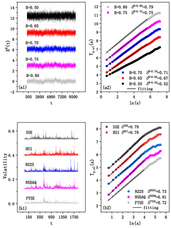
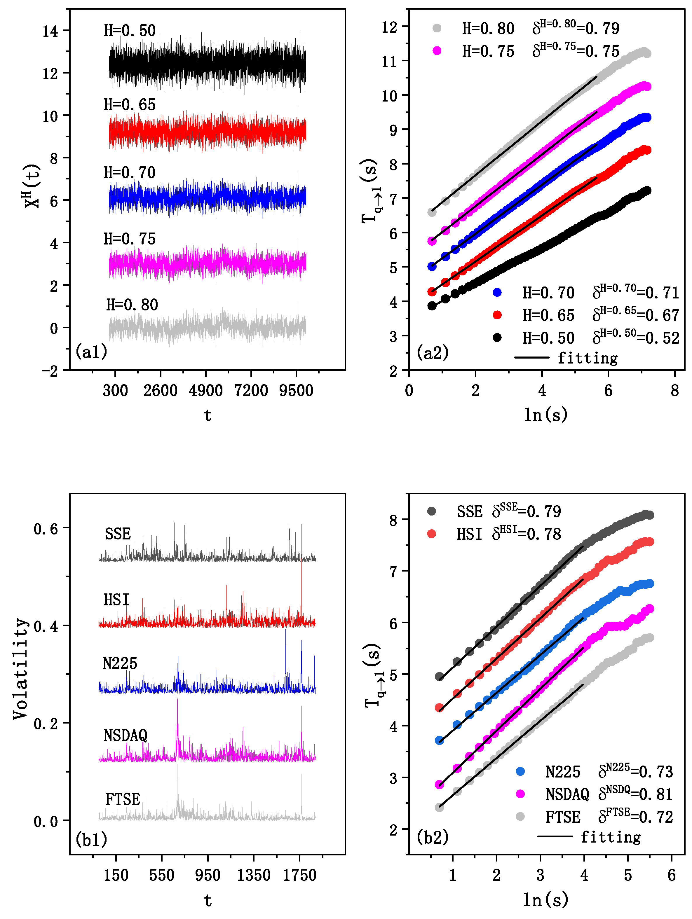
In Figure 1, five samples of increment series generated with $H=0.50,0.65,0.70,0.75$ and $0.80$ are shown in Figure 1(a1).The length is chosen to be $N={10}^4$. The curves of diffusion entropy versus logarithm of scale in Figure 1(a2) turn out to obey the linear relation in Equation (4), namely, ${lim}_{q\to 1}{T}_q\left(s\right)=const+\delta lns$, the slopes of which read $\delta =0.52,0.67,0.71,0.75$ and $0.79$, being almost identical with their corresponding Hurst exponents $H=0.50,0.65,0.70,0.75$, and $0.80$, just as expected by theory. Hence, the qualities of the generated increment series are good enough.

Figure 1. Materials and their long-term persistent behaviors. (a1) Five samples of increment series generated with the fractional Brownian motion model. (b1) The curves of diffusion entropy versus the logarithm of scale for the samples of increment series in panel (a1), the slopes of which are almost identical to the corresponding Hurst exponents. (a2) The daily volatility series of five stock exchange markets. (b2) The curves of diffusion entropy versus the logarithm of scale. For visual convenience, the curves are shifted vertically.

The constructed volatility series are displayed in Figure 1(b1),whose curves of diffusion entropy versus logarithm of scale also perfectly obey the linear relation in Equation (4), i.e., the volatility series all demonstrate significant long-term persistence, as shown in Figure 1(b2).The slopes, i.e., the scaling exponents, read $\left({\delta }^{\mathrm{SSE}},{\delta }^{\mathrm{HSI}},{\delta }^{\mathrm{N}225},{\delta }^{\mathrm{NSDQ}},{\delta }^{\mathrm{FTSE}}\right)=\left(0.79,0.78,0.73,0.81,0.72\right)$.

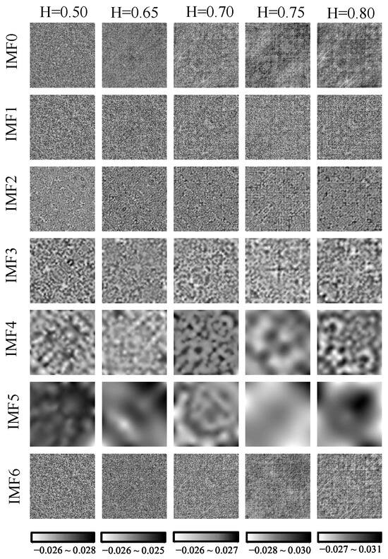
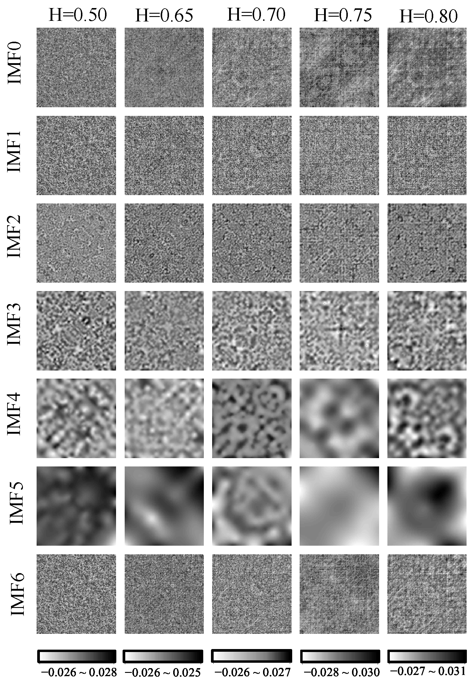
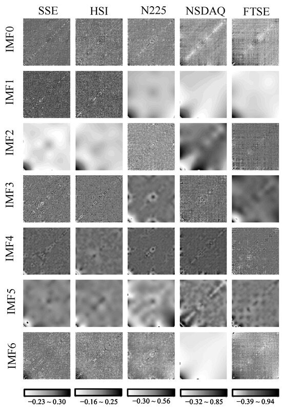
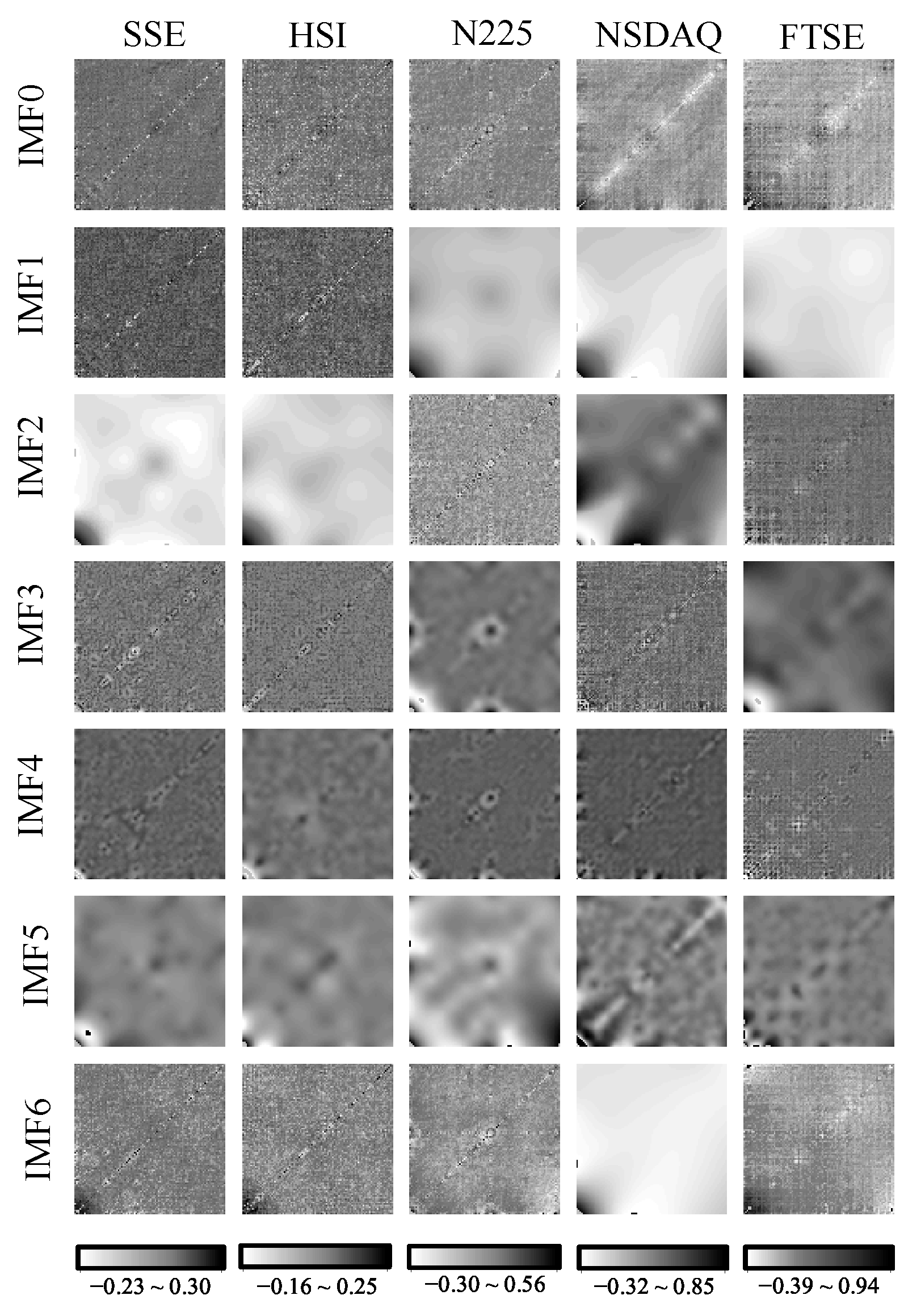
The patterns for the original correlations $IM{F}_0$, the components (from $IM{F}_1$ to $IM{F}_5$), and the reconstructed correlations ($IM{F}_6$) in the five samples of the increment series generated with the fBm model and in the five volatility series for the stock markets are displayed in Figure 2 and Figure 3, respectively. The contributions of the components are listed in Table 1.

Figure 2. The IMFs for the increment series generated with the fractional Brownian motion model presented in Figure 1.

Figure 3. The IMFs for the volatility series for SSE, HSI, N225,NASDQ, and FTSE, as displayed in Figure 1.

Table 1. Contributions of each IMF component for different H values (upper panel) and various stock indices (lower panel).

	IMF1	IMF2	IMF3	IMF4	IMF5
H = 0.50	0.89	0.07	0.02	0.01	0.01
H = 0.65	0.71	0.15	0.07	0.04	0.03
H = 0.70	0.63	0.16	0.11	0.07	0.03
H = 0.75	0.47	0.18	0.13	0.12	0.10
H = 0.80	0.43	0.20	0.17	0.13	0.07
SSE	0.50	0.16	0.16	0.10	0.08
HSI	0.54	0.18	0.14	0.08	0.06
N225	0.28	0.22	0.21	0.15	0.14
NSDQ	0.78	0.11	0.05	0.03	0.03
FTSE	0.49	0.30	0.09	0.07	0.05

Theoretically, in the case of $H=0.5$, there should be no macroscopic patterns indicating long-term persistence; however, we can find the macroscopic ones exposed in the $IM{F}_3,IM{F}_4$, and $IM{F}_5$ with limited contributions of $(2\%,1\%,1\%)$, which are filtered out (ignored) in the reconstructed landscape $IM{F}_6$. With the increase in the Hurst exponent from $0.5$ to $0.80$, the contribution for the $IM{F}_1$ decreases from $89\%$ to $43\%$, while that for the $IM{F}_2,IM{F}_3$, and $IM{F}_4$ increase monotonically from $7\%,2\%,1\%$ to $20\%,17\%,13\%$, respectively. The contributions of the macroscopic patterns in $IM{F}_5$ are all less than $10\%$, being discarded in all the reconstructed correlations. Hence, the contributions of the macroscopic patterns stored in $IM{F}_3$, $IM{F}_4$, and $IM{F}_5$ become progressively larger and are subsequently preserved in the constructed ones ($IM{F}_6$). A simple comparison shows that the component with the largest contribution ($IM{F}_1$) extracts the microscopic patterns, storing no differences between the samples.

The scaling exponents of long-term persistence for the $SSE,HSI$, and $NSDQ$ are in the range of $\delta \in [0.78,0.81]$. The contributions of their $IM{F}_1$ ($50\%,54\%$, and $78\%$), are significantly large, being out of the interval of $[43\%,47\%]$ for the increment series generated with $H\in [0.75,0.8]$. The scaling exponents of long-term persistence for $N225$ and $FTSE$ are $0.73$ and $0.72$. The contributions of their $IM{F}_1$ ($28\%$ and $49\%$) are significantly small/large, being out of the interval of $[47\%,63\%]$ for the increment series generated with $H=[0.70,0.75]$. What is more, the components with the largest contributions ($IM{F}_1$ and $IM{F}_2$) in the volatility series for the stock markets are dominated by macroscopic structures, whereas those for the fBm increment series are dominated by microscopic structures. Hence, the fBm model can not reproduce the rich patterns in the three-point correlations in volatility series for stock markets.

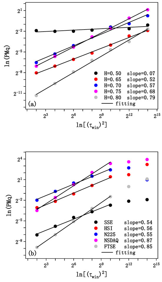
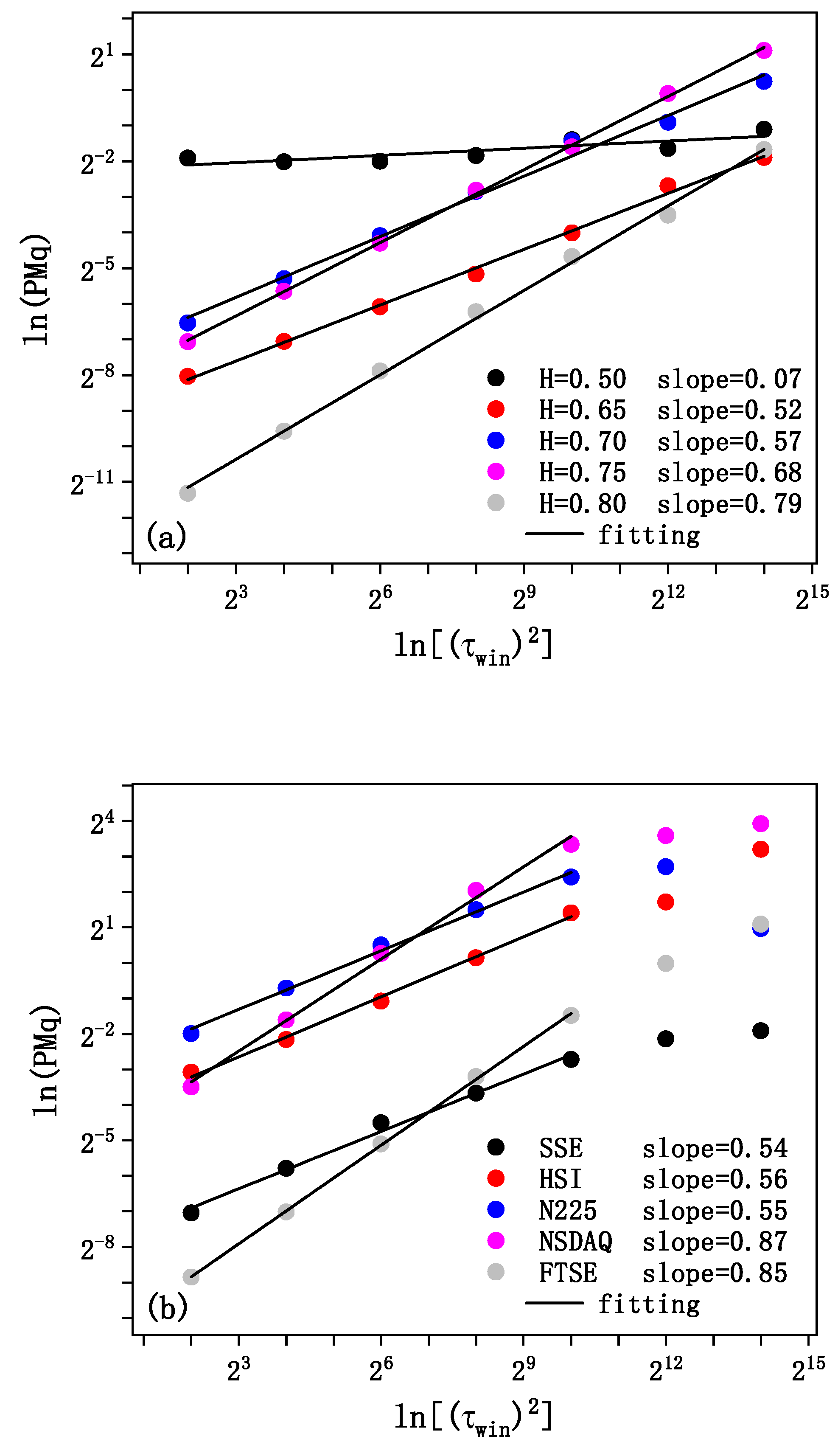
As displayed by the power-laws in Figure 4, the $IM{F}_0$s for all the increment series generated with the fBm model turn out to have fractal structures, with the slopes (fractal dimensions) corresponding to $H=0.50,0.65,0.70,0.75$, and $0.80$ being $h\left(2\right)=0.07,0.52,0.57,0.68$, and $0.79$, respectively (see Figure 4a). The fractal dimension increases monotonically with the Hurst exponent. The $IM{F}_0$s for the volatility serie also have perfect fractal structures, with the fractal dimensions corresponding to $SSE$, $HSI$, $N225$, $NSDQ$, and $FTSE$ being $h\left(2\right)=0.54,0.56,0.55,0.87$, and $0.85$, respectively (see Figure 4b). The scaling values of long-term persistence for $SSE,HSI$ and $NSDQ$ are $\sim 0.80$ (see panel (b2) in Figure 1), but their fractal dimensions are $h\left(2\right)=0.54,0.56,0.87$, being out of the interval of $h\left(2\right)\in [0.68,0.79]$ corresponding to $H\in [0.75,0.80]$. And the scaling value of long-term persistence for $FTSE$ is $0.72$ (see panel (b2) in Figure 1), but its fractal dimension reads $0.85$, being significantly large and out of the interval $[0.57,0.68]$ corresponding to the increment series with $H\in [0.70,0.75]$. Hence, the fBm model can reproduce qualitatively the fractal structure in volatility series but can not correctly give the quantitative value of the fractal dimension.

Figure 4. The power-laws (a) The scaling behaviors of the original three-point correlations in the increment series with $H=0.5,0.65,0.70,0.75$, and $0.80$. (b) The scaling behaviors of the original three-point correlations in the daily volatility series with five stock exchange markets.

Table 2 presents the topological characteristics of the correlation networks for the original landscapes of $IM{F}_0$ and the reconstructed ones of $IM{F}_6$. From the component contributions displayed in Figure 3 one can find that the reconstructed correlation $IM{F}_6$ for the volatility series of $NSDQ$ is dominated with a macroscopic structure of a large scale. Its network turns out to compose of few edges. Hence, its corresponding characteristics are marked with “N/A”. Herein, we also compare the characteristics for $SSE,HSI$, and $NSDQ$ with that for increment series generated with $H\in [0.75,0.80]$, and for the $N225$ and $FTSE$ with that for the increment series generated with $H=\in [0.7,0.75]$ (called expected characteristics).

Table 2. Topological characteristics.

	Average Degree		Clustering Coefficient		Closeness		Modularity
	IMF0	IMF6	IMF0	IMF6	IMF0	IMF6	IMF0	IMF6
H = 0.50	5.02	4.86	0.06	0.05	3.59	3.65	0.35	0.37
H = 0.65	4.68	5.00	0.05	0.04	3.67	3.56	0.36	0.30
H = 0.70	4.43	4.89	0.05	0.04	3.85	3.60	0.37	0.35
H = 0.75	3.87	3.92	0.05	0.05	4.01	3.97	0.37	0.34
H = 0.80	3.79	3.87	0.05	0.04	3.97	3.98	0.38	0.32
SSE	4.63	4.76	0.12	0.12	3.66	3.57	0.40	0.41
HSI	4.73	4.99	0.10	0.12	3.56	3.53	0.35	0.36
N225	4.30	3.23	0.08	0.09	3.94	4.51	0.45	0.45
NSDQ	3.91	N/A	0.06	N/A	3.93	N/A	0.42	N/A
FTSE	4.04	3.53	0.18	0.17	3.61	3.75	0.38	0.38

The findings include three items. (i) With the decrease in H, the average degrees for the original and reconstructed correlations decrease monotonically, respectively. The other characteristics are independent of H. (ii) The average degrees for both the original and the reconstructed correlation networks are significantly larger than the corresponding expected values, respectively, (see the first column in Table 2). (iii) The average clustering coefficients for the original and the reconstructed correlation networks are significantly larger than the corresponding expected values, respectively (see the second column in Table 2). Accordingly, we conclude that the fBm model can not reproduce the topological characteristics.

5. A Brief Summary

Multiple-point correlation is a powerful tool to expose fine structures in multi-dimensional landscapes. In this work, it is extended to display the fine structures of correlations in mono-variate time series, which have been accounted for by means of the high-order moments or probability moments in current time series analysis, but in an average way, i.e., the fine structures are lost in the procedure of statistical average.

As a typical example, we detect the three-point correlations in volatility series of daily closing prices for five important stock exchange markets distributed in Asia, America, and Europe, and to understand them better, we display the three-point correlations in increment series generated with the fBm model to setup a reference. In the fBm time series, a stronger long-term persistence induces macroscopic patterns with larger contributions to the original correlation. And the original correlation turns out to have a fractal structure, the fractal dimension for which increases monotonically with the Hurst exponent. The values of the Hurst exponent for the five volatility series, detected with the diffusion entropy, are $0.79$ (SSE), $0.78$ (HSI), $0.73$ (N225), $0.81$ (NSDQ), and $0.72$ (FTSE), respectively, for the stock market indices. The contributions of the components in these empirical series differ considerably from that for fBm increment series generated with identical Hurst exponents. The fractal structures in the original correlations for the empirical records can be reproduced with the fBm model, but their quantitative behaviors are different. And the topological behaviors for the correlations and reconstructed correlations for the empirical records differ significantly with that for the fBm increment series. Consequently, the fBm model can not reproduce the rich patterns in the three-point correlations in volatility series for stock markets.

In contemporary financial research, fBm is extensively employed to delineate stock markets. Nevertheless, the present study posits that fBm is overly idealized and deviates considerably from the behavior of real financial markets. For instance, fBm does not correspond to the quantitative fractal dimensions and network topological patterns exhibited by actual markets. Consequently, the utilization of fBm for empirical studies, such as risk analysis, will yield results that diverge from reality. By identifying the specific discrepancies between fBm and actual markets, including differences in component contributions, fractal dimensions, and network topology, the present study provides a theoretical and numerical basis for further improving volatility models. These findings can be utilized by researchers to calibrate more realistic models and to better assess the limitations of fBm-based predictions.

Hence, the three-point correlation can provide us with detailed knowledge on what characteristics in empirical records can be or cannot be reproduced with theoretical models. However, the present study has not yet been extended to higher-order correlations, which are expected to encode more intricate information. Obviously, extensive calculations for financial time series are useful to reach a general picture of the MPC in financial markets, and the benchmark (fBm) needs to be revised, which will be conducted in our future works.

References

- Pearson, K. Mathematical Contributions to the Theory of Evolution. III. Regression, Heredity, and Panmixia. Philos. Trans. R. Soc. Lond. Ser. A 1896, 187, 253–318. [Google Scholar]
- Tsallis, C. Possible generalization of boltzmann-gibbs statistics. J. Stat. Phys. 1988, 52, 479–487. [Google Scholar] [CrossRef] [Scilit]
- Mandelbrot, B. Multifractal measures, especially for geophysicist. Pure Appl. Geophys. 1989, 131, 5–42. [Google Scholar] [CrossRef] [Scilit]
- Jaffard, S. Multifractal formalism for functions. I. Results valid for all functions. II. Self-similar functions. SIAM J. Math. Anal. 1997, 28, 944–998. [Google Scholar]
- Scafetta, N.; Grigolini, P. Scaling detection in time series: Diffusion entropy analysis. Phys. Rev. E 2002, 66, 036130. [Google Scholar] [CrossRef] [Scilit]
- Zhang, W.Q.; Qiu, L.; Xiao, Q.; Yang, H.J.; Zhang, Q.J.; Wang, J.Y. Evaluation of scale invariance in physiological signals by means of balanced estimation of diffusion entropy. Phys. Rev. E 2012, 86, 056107. [Google Scholar] [CrossRef] [Scilit]
- Cover, T.M.; Thomas, J.A. Elements of Information Theory; Wiley: New York, NY, USA, 1991. [Google Scholar]
- Schreiber, T. Measuring Information Transfer. Phys. Rev. Lett. 2000, 85, 461. [Google Scholar] [CrossRef] [Scilit]
- Peng, C.-K.; Buldyrev, S.V.; Havlin, S.; Simons, M.; Stanley, H.E.; Goldberger, A.L. Mosaic organization of DNA nucleotides. Phys. Rev. E 1994, 49, 1685. [Google Scholar] [CrossRef] [Scilit]
- Kantelhardt, J.W.; Zschiegner, S.A.; Koscielny-Bunde, E.; Havlin, S.; Bunde, A.; Stanley, H.E. Multifractal detrended fluctuation analysis of nonstationary time series. Phys. A Stat. Mech. Its Appl. 2002, 316, 87–114. [Google Scholar] [CrossRef] [Scilit]
- Blackledge, J.; Lamphiere, M. A Review of the Fractal Market Hypothesis for Trading and Market Price Prediction. Mathematics 2022, 10, 117. [Google Scholar] [CrossRef] [Scilit]
- Mandelbrot, B.B. The Fractal Geometry of Nature; W. H. Freeman and Co.: New York, NY, USA, 1982; ISBN 0-7167-1186-9. [Google Scholar]
- Anderson, N.; Noss, J. The Fractal Market Hypothesis and its implications for the stability of financial markets. Financ. Stabil. 2013, 3, 3–22. [Google Scholar]
- Torquato, S. Random Heterogeneous Materials: Microstructure and Macroscopic Properties; Springer: New York, NY, USA, 2002. [Google Scholar]
- Garrett-Roe, S.; Hamm, P. Three-point frequency fluctuation correlation functions of the OH stretch in liquid water. J. Chem. Phys. 2008, 128, 104507. [Google Scholar] [CrossRef] [Scilit] [PubMed]
- Berryman, J.G. Interpolating and integrating three-point correlation functions on a lattice. J. Comput. Phys. 1988, 75, 86–102. [Google Scholar] [CrossRef] [Scilit]
- Hwang, K.; Schmittmann, B.; Zia, R.K.P. Three-point correlation functions in uniformly and randomly driven diffusive systems. Phys. Rev. E 1993, 48, 800–809. [Google Scholar] [CrossRef] [Scilit]
- Šanda, F.; Mukamel, S. Multipoint correlation functions for continuous-time random walk models of anomalous diffusion. Phys. Rev. E 2005, 72, 031108. [Google Scholar] [CrossRef] [Scilit]
- Moore, A.W.; Connolly, A.J.; Genovese, C.; Gray, A.; Grone, L.; Kanidoris, N., II; Nichol, R.C.; Schneider, J.; Szalay, A.S.; Szapudi, I.; et al. Fast algorithms and efficient statistics: N-point correlation functions. In Mining the Sky: Proceedings of the MPA/ESO/MPE Workshop Held at Garching, Germany, 31 July–4 August 2000; Banday, A.J., Zaroubi, S., Bartelmann, M., Eds.; ESO Astrophysics Symposia; Springer: Berlin/Heidelberg, Germany, 2001; pp. 71–82. [Google Scholar]
- Grech, D.; Pamuła, G. New measure of multifractality and its application in finances. arXiv 2013, arXiv:1309.5466. [Google Scholar] [CrossRef] [Scilit]
- Huang, N.E.; Shen, Z.; Long, S.R.; Wu, N.C.; Shih, H.H.; Zheng, Q.; Yend, N.C.; Tung, C.C.; Liu, H.H. The empirical mode decomposition and the Hilbert spectrum for nonlinear and non-stationary time series analysis. Proc. R. Soc. A Math. Phys. Eng. Sci. 1998, 454, 903–995. [Google Scholar] [CrossRef] [Scilit]
- Xu, Y.; Liu, B.; Liu, J.; Riemenschneider, S. Two-dimensional empirical mode decomposition by finite elements. Proc. R. Soc. A Math. Phys. Eng. Sci. 2006, 462, 3081–3096. [Google Scholar] [CrossRef] [Scilit]
- Karperien, A.L.; Jelinek, H.F. Box-Counting Fractal Analysis: A Primer for the Clinician. In The Fractal Geometry of the Brain; Advances in Neurobiology; Di Ieva, A., Ed.; Springer: Cham, Switzerland, 2024; Volume 36. [Google Scholar]
- Albert, R.; Barabasi, A.-L. Statistical mechanics of complex networks. Rev. Mod. Phys. 2002, 74, 47–97. [Google Scholar] [CrossRef] [Scilit]
- Newman, M.E.J.; Girvan, M. Finding and evaluating community structure in networks. Phys. Rev. E 2004, 69, 026113. [Google Scholar] [CrossRef] [Scilit] [PubMed]
- Mandelbrot, B.; Van Ness, J.W. Fractional Brownian motions: Fractional noises and applications. SIAM Rev. 1968, 10, 422–437. [Google Scholar] [CrossRef] [Scilit]
- Available online: https://cn.investing.com (accessed on 28 September 2025).
- Wright, J.H. Log-Periodogram Estimation of Long Memory Volatility Dependencies with Conditionally Heavy Tailed Returns; Board of Governors of the Federal Reserve System: Washington, DC, USA, 2000.
Disclaimer/Publisher’s Note: The statements, opinions and data contained in all publications are solely those of the individual author(s) and contributor(s) and not of MDPI and/or the editor(s). MDPI and/or the editor(s) disclaim responsibility for any injury to people or property resulting from any ideas, methods, instructions or products referred to in the content. |
© 2026 by the authors. Licensee MDPI, Basel, Switzerland. This article is an open access article distributed under the terms and conditions of the Creative Commons Attribution (CC BY) license.