Copulas for Stochastic Volatility Models

Abstract

In this article, a Fokker–Planck equation framework for the copula density associated with a two-dimensional stochastic differential equations system is developed. The different information pieces associated with the statistical interdependence properties and the marginal ones are separated explicitly, and the corresponding boundary conditions for the copula distribution are analyzed. Given the set of functions that defines the copula density dynamics and the marginal probability density functions, a Fokker-Planck equation for the multivariate density probability function of the stochastic volatility model is obtained.

1. Introduction

A key problem in finance is to understand how the assets in a portfolio are intermingled from a statistical point of view, i.e., to determine what the dependence is between the returns of the different random variables that make up the portfolio. A typical measure of the dependence between a pair of random variables is the correlation coefficient $\rho$, or in the general case of n assets, the correlation matrix ${\rho }_{ij}$ [1,2,3]. It is now clear that the correlation coefficient is only one of the possible measures of dependence [4], and this parameter is insufficient to provide a complete description of the dependence between two assets [5,6].

Also, in financial economics it is central to characterise how asset returns, volatilities, and other state variables co-move over time. In many applications, the dependence structure is at least as important as the marginal dynamics. Portfolio allocation, derivative pricing, contagion analysis, systemic-risk measurement, and stress testing all require an adequate representation of joint behaviour, especially when dependence is non-linear, asymmetric, state-dependent, or time-varying. Traditional summaries such as linear correlation are often insufficient for this task because they provide only a partial description of statistical dependence and do not generally identify tail co-movement, non-linear association, or the way dependence evolves jointly with the underlying stochastic system.

Thus, it is necessary to retain all the information contained in the complete joint multivariate distribution of the random variables under study. The notion of copula associated with the multivariate distribution [7,8,9,10,11] provides a natural framework for separating marginal behaviour from dependence without information loss. By Sklar’s theorem [12,13,14] any multivariate distribution may be decomposed into its marginal distributions and a copula that captures the dependence structure linking them. This decomposition has made copulas a standard tool in finance, econometrics, and statistics, where they are used to model joint distributions flexibly without imposing restrictive joint normality assumptions. Applications of copula theory range from statistics [15], finance and time-series (where copulas have been employed to study exchange-rate dependence, volatility spillovers, systemic risk, and dynamic cross-market linkages) [16,17,18,19,20,21,22,23], econometrics [24,25], economics [26,27], cryptoanalysis [28], forexmarket [29], geophysics [30,31,32,33,34], and quantum security [35].

The typical families of copulas: Gaussian, Student, Archimedean, Gumbel, Clayton, etc. [7,8] are all time–independent, but there are efforts to incorporate time dependence in the copula [36,37,38,39] as well as their application to stochastic volatility models [40]. More recently, the literature has developed increasingly flexible time-varying and high-dimensional copula constructions, including vine and factor copulas, to accommodate richer temporal and cross-sectional dependence patterns [41,42,43].

Despite this progress, a conceptual gap remains. Most empirical copula models specify the dependence structure either statically or through exogenous parameter dynamics. In those approaches, the copula is introduced as an additional layer on top of the stochastic model, rather than being derived from the same probabilistic mechanism that governs the evolution of the underlying state variables. By contrast, when the primitive model is a multidimensional diffusion, the joint transition density evolves according to a Fokker–Planck equation [44]. Thus, in this direction [45] use a Fokker–Planck scheme to determine the copula.

For a given set of random variables (whose statistical properties are defined by their multivariate distribution function), Sklar’s theorem allows us to separate the interdependence properties between these variables (the copula) from the marginal distributions and, in addition, to reconstruct the multivariate distribution function from these two independent sets of information. Now, in the time-dependent continuous case, a set of random variables $X_i$ is defined by means of a system of stochastic differential equations

$$d{X}_i={\mu }_i(X_j,t)dt+{\displaystyle \sum _{\begin{array}{c}j=1\end{array}}^N}{\sigma }_{ij}(X_j,t)d{W}_i$$

with

$$d{W}_{i}d{W}_j={\delta }_{ij}dt$$

where $d{W}_i$ are Wiener processes. This system is equivalent to a Fokker–Planck equation [46] for the multivariate probability density function $f(\overrightarrow{x},t)=f(x_1,x_2,\dots ,x_n,t)$ given by

$${\displaystyle \frac{\partial }{\partial t}}f(\overrightarrow{x},t)=-{\displaystyle \sum _{i=1}^n}{\displaystyle \frac{\partial }{\partial x_i}}\left[{\mu }_i(\overrightarrow{x},t)f(\overrightarrow{x},t)\right]+{\displaystyle \frac{1}{2}}{\displaystyle \sum _{i,j=1}^n}{\displaystyle \frac{{\partial }^2}{\partial x_i\partial x_j}}\left[{\Sigma }_{ij}(\overrightarrow{x},t)f(\overrightarrow{x},t)\right]$$

(1)

where the matrix $\Sigma$ is

$$\Sigma (\overrightarrow{x},t)=\sigma (\overrightarrow{x},t){\sigma }^t(\overrightarrow{x},t).$$

In the standard Fokker–Planck equation description given by Equation (1), the interdependence and marginal properties are interrelated, and there is no clear separation between them. This raises a natural and, to our knowledge, insufficiently explored question: can one derive directly a dynamical equation for the copula density itself, thereby separating the evolution of dependence from the evolution of the marginals at the level of the governing partial differential equation?

This paper addresses that question for a two-dimensional diffusion system, with stochastic volatility models as the leading application. Specifically, we consider a bivariate Itô diffusion for an asset price and its volatility, derive the associated Fokker–Planck equation for the joint density, and then perform a copula-based change of variables from the original state space to copula coordinates. This transformation allows us to obtain a partial differential equation for the copula density itself. The resulting copula–Fokker–Planck equation provides an explicit dynamical representation of dependence, separate from but linked to the marginal laws of the underlying variables.

Our objective is not merely formal. The proposed framework clarifies how dependence enters the dynamics of stochastic-volatility systems, how marginal distributions and copula evolution interact, and how boundary conditions should be formulated once the problem is mapped to the compact copula domain $[0,1]\times [0,1]$. This is especially relevant in finance, where the dependence between returns and volatility is often interpreted through instantaneous correlation parameters, even though broader forms of dependence may arise from the full non-linear structure of the diffusion and its induced joint law. A PDE-based copula representation makes these mechanisms transparent and provides a systematic analytical tool for studying dynamic dependence beyond Gaussian or elliptical benchmarks.

The paper is related to, but distinct from, several strands of the literature. First, classical copula models in finance typically focus on flexible static families or on dynamic specifications in which time variation is introduced through evolving copula parameters [16]. These contributions are extremely useful empirically, but they do not derive copula dynamics from the underlying diffusion law itself. Second, recent work on high-dimensional dependence, including vine copulas and structured factor copulas, has considerably expanded the scope of feasible dependence modelling in time series and systemic-risk applications [41,42,43]. However, these papers study flexible copula constructions for multivariate dependence and forecasting rather than deriving a Fokker–Planck-type equation for the copula density associated with a continuous-time stochastic-volatility model. Third, the stochastic-volatility literature, beginning with canonical models such as Heston [47], focuses primarily on pricing, filtering, and implied-volatility dynamics, with the dependence between state variables typically encoded through instantaneous covariance terms. Our approach is different: we use the diffusion model as the starting point for deriving an explicit evolution equation for the copula density, thereby isolating and interpreting the dynamics of dependence in their own right.

Contribution Paragraph

The main contribution of the paper is therefore twofold. First, at the theoretical level, we derive an explicit partial differential equation for the copula density associated with a general two-dimensional diffusion process. The derivation shows how the coefficients of the original stochastic differential system, together with the marginal densities and their derivatives, determine the drift, diffusion, and lower-order terms of the copula dynamics. We also make explicit the domain of the transformed problem and discuss the corresponding boundary conditions on the unit square.

Second, at the applied level, the framework provides a systematic way to study dynamic dependence in stochastic-volatility models beyond standard parametric copula families. Rather than imposing a copula ex ante, the method derives the dependence dynamics implied by the primitive diffusion itself. This makes it possible, at least in principle, to compare instantaneous correlation with the richer dependence structure generated by nonlinear drift and diffusion terms, and to analyze settings in which zero instantaneous correlation does not imply independence of the resulting copula.

The paper also has methodological value. By working at the PDE level, we obtain a representation that is transparent enough to support both analytical inspection and future numerical implementation. In particular, the transformed equation reveals directly which terms correspond to diffusion in copula coordinates, which terms are inherited from the marginal transformations, and how the original stochastic-volatility specification shapes the evolution of dependence. This interpretation would be difficult to obtain from the joint Fokker–Planck equation alone, where marginal and dependence effects are entangled.

At the same time, the scope of the paper should be stated clearly. We work in the two-dimensional continuous-diffusion setting and emphasize analytical structure rather than empirical calibration. Accordingly, the paper is best viewed as a foundational contribution: it develops the mathematical framework needed to analyze copula dynamics induced by diffusion systems and illustrates its relevance in stochastic-volatility environments. Extensions to higher dimensional systems, numerical schemes, calibration strategies, and empirical performance assessment are important topics, but they lie beyond the present paper and are left for future research.

The remainder of the paper is organized as follows. Section 2 introduces the stochastic volatility framework and the corresponding joint Fokker–Planck equation. Section 3 offers a concise literature review of efforts to introduce time dependence into the copula. Section 4 derives the copula–Fokker–Planck equation through a change of variables from the original state space to copula coordinates. Section 5 presents the standing assumptions underlying the derivations and discusses the boundary conditions on the compact domain $[0,1]\times [0,1]$. Section 6 examines the uncorrelated case and clarifies why zero instantaneous correlation does not, in general, imply copula independence. Section 7 concludes.

2. Volatility Models and the Fokker–Planck Equation

Consider a generic stochastic volatility model that is characterized in continuous time by two coupled stochastic differential equations for the underlying asset price S and the volatility $\sigma$ of the form [48,49]

$$dS=\mu (S,\sigma ,t)dt+G(S,\sigma ,t)d{W}_S\left(t\right)$$

(2)

$$d\sigma =r(S,\sigma ,t)dt+q(S,\sigma ,t)d{W}_{\sigma }\left(t\right)$$

(3)

where $\mu ,G,r$ and q are arbitrary functions of $S,\sigma$ and t that defines the stochastic volatility model completely. The two Brownian motions $d{W}_S$ and $d{W}_{\sigma }$ satisfy the product rule

$$d{W}_{S}d{W}_{\sigma }=\rho dt$$

(4)

in Itô’s sense, and the parameter $-1\le \rho \le 1$ is called the correlation parameter. Between the different plethora of models, the best known are the Heston model [47], the Ornstein–Uhlenbeck model [48], the CEV model [50,51], the SABR volatility model [52], the Hull and White model [53], and the Chen model [54].

The transition probability density $p=p\left(t^{\prime },S^{\prime },{\sigma }^{\prime }|t,S,\sigma \right)$ for the stochastic differential Equations (2) and (3) satisfies the Fokker–Planck equation [46]

$${\displaystyle \frac{\partial p}{\partial t}}={\displaystyle \frac{1}{2}}{\displaystyle \frac{{\partial }^2\left(G^{2}p\right)}{\partial S^2}}+\rho {\displaystyle \frac{{\partial }^2\left(Gqp\right)}{\partial S\partial \sigma }}+{\displaystyle \frac{1}{2}}{\displaystyle \frac{{\partial }^2\left(q^{2}p\right)}{\partial {\sigma }^2}}-{\displaystyle \frac{\partial \left(\mu p\right)}{\partial S}}-{\displaystyle \frac{\partial \left(rp\right)}{\partial \sigma }}$$

(5)

It is convenient to separate the Fokker–Planck Equation (5) into three types of terms: (i) Kinetic: associated with second-order differential operators, (ii) Magnetic: related to first-order differential operators, (iii) Electric: generated by a multiplicative potential term in the form

$${\displaystyle \frac{\partial p}{\partial t}}={\displaystyle \frac{1}{2}}{G}^2{\displaystyle \frac{{\partial }^{2}p}{\partial S^2}}+\rho Gq{\displaystyle \frac{{\partial }^{2}p}{\partial S\partial \sigma }}+{\displaystyle \frac{1}{2}}{q}^2{\displaystyle \frac{{\partial }^{2}p}{\partial {\sigma }^2}}-A_S{\displaystyle \frac{\partial p}{\partial S}}-A_{\sigma }{\displaystyle \frac{\partial p}{\partial \sigma }}+\Phi p(s,\sigma ,t)$$

(6)

where the magnetic potential terms are given by

$$A_S=A_S(S,\sigma ,t)=\mu -{\displaystyle \frac{\partial \left(G^2\right)}{\partial S}}-\rho {\displaystyle \frac{\partial \left(Gq\right)}{\partial \sigma }}$$

(7)

$$A_{\sigma }=A_{\sigma }(S,\sigma ,t)=r-{\displaystyle \frac{\partial \left(q^2\right)}{\partial \sigma }}-\rho {\displaystyle \frac{\partial \left(Gq\right)}{\partial S}}$$

(8)

and the electric potential is

$$\Phi =\Phi (s,\sigma ,t)=-{\displaystyle \frac{\partial \left(\mu \right)}{\partial S}}-{\displaystyle \frac{\partial \left(r\right)}{\partial \sigma }}+{\displaystyle \frac{1}{2}}{\displaystyle \frac{{\partial }^2\left(G^2\right)}{\partial S^2}}+{\displaystyle \frac{1}{2}}{\displaystyle \frac{{\partial }^2\left(q^2\right)}{\partial {\sigma }^2}}+\rho {\displaystyle \frac{{\partial }^2\left(Gq\right)}{\partial S\partial \sigma }}$$

(9)

The terms Kinetic, Magnetic, and Electric are derived from the analogy between the Fokker–Planck Equation (6) and the Schrödinger equation for a particle of mass m and charge q in an external electromagnetic field:

$$i\hslash {\displaystyle \frac{\partial \psi }{\partial t}}={\displaystyle \frac{-{\hslash }^2}{2m}}{\overrightarrow{\nabla }}^2\psi +{\displaystyle \frac{iq\hslash }{mc}}\overrightarrow{\mathit{A}}·\overrightarrow{\nabla }\psi +{\displaystyle \frac{q^2}{2m{c}^2}}{\overrightarrow{\mathit{A}}}^2\psi +q\Phi \psi$$

Here, $\overrightarrow{\mathit{A}}$ denotes the magnetic vector potential, and $\Phi$ represents the external electric potential.

3. Close Literature Review

There is little literature on copula densities and the Fokker–Planck equation. An interesting article on this topic and on which we base our proposal is [45], which analyses a special stochastic two-dimensional stochastic differential system (called inference function for margins or IFM) associated with the asset prices $S_1$ and $S_2$ of the form:

$$\left\{\begin{array}{c}d{S}_1=b_1\left(S_1,t\right)dt+{\sigma }_{11}\left(S_1,t\right)d{w}_1+{\sigma }_{12}\left(S_1,t\right)d{w}_2\hfill \\ d{S}_2=b_2\left(S_2,t\right)dt+{\sigma }_{21}\left(S_2,t\right)d{w}_2+{\sigma }_{22}\left(S_2,t\right)d{w}_3\hfill \end{array}\right.$$

(10)

In that paper, an equation for the copula distribution function $C(u,v)$ is derived from an integro-differential Fokker–Planck equation. Note that the price variables in (10) evolve independently, although they are correlated.

Here we follow a similar idea, but

(i)

In terms of the copula density function $c(u,v,t)$ instead of the Copula distribution $C(u,v)$ and

(ii)

We consider a general two-dimensional stochastic system associated with the generic stochastic volatility model (2) and (3), in which the asset price S and the volatility $\sigma$ are not independent variables.

This will allow us to find a Fokker–Planck equation associated with the copula density $c(u,v)$ and to study its consequences more straightforwardly.

A key point of departure from [45] should be emphasized clearly. Their analysis develops an integro-differential equation for the copula distribution function $C(u,v,t)$, whereas our paper derives a genuine partial differential equation for the copula density $c(u,v,t)$. This distinction is substantive rather than notational. By working directly at the density level, our framework permits the dependence structure to be written in a standard Fokker–Planck form and makes it possible to identify transformed coefficients and potentials that govern the copula dynamics at the level of the differential operator. In this sense, the contribution of the present paper is not a re-derivation of [45], but an extension that shifts the analysis from a distribution-based representation to a density-based dynamical framework. This representation is especially useful because it allows two complementary perspectives: starting from a joint diffusion, one may extract the implied time-varying copula-density dynamics; conversely, starting from an admissible copula-density evolution together with given marginals, one may reconstruct a consistent joint Fokker–Planck equation. The resulting formulation provides a more direct analytical connection between copula dependence, stochastic-volatility modelling, and the operator structure of the associated diffusion system.

The preceding results admit two complementary interpretations that help clarify the role of time dependence in our framework. First, in a top-down reading, one starts from a given joint diffusion system and its associated Fokker–Planck equation; in that case, Theorem 1 shows how the implied time-varying copula density can be extracted from the joint dynamics. Second, in a bottom-up reading, one starts from an admissible evolution equation for the copula density, together with given marginal densities, and Corollary 1 allows one to reconstruct a consistent joint Fokker–Planck equation. In this sense, the framework is bi-directional. At the same time, the term “independent” used in connection with the copula equation should be interpreted carefully: it does not mean that the copula is conceptually detached from the marginals under Sklar’s theorem, but rather that, after the change of variables and the introduction of the transformed coefficients, the governing differential operator for the copula density can be written in a decoupled form. The contribution is therefore an operator-level separation of dependence dynamics from marginal dynamics, not a claim that the full probabilistic structure ceases to link them.

An interesting time-dependent copula analysis, but not in a Fokker–Planck context, can be found in [41,42,43]. In [41], a time-varying copula method is developed to model the dependence structure among financial sectors. By incorporating market-specific weights and Archimedean copula-based correlations, this model accounts for nonlinear dependencies across financial segments. Ref. [42] employs Credit Default Swaps (CDS) to model the joint and conditional distress probabilities of banks in Europe and the U.S. using factor copulas. Here, multi-factor, structured factor, and factor-vine models are proposed. In [43], a computationally efficient method is developed to estimate, simulate, and predict dependencies across variables and time points using Vine copulas.

Whereas these studies are useful, our aim is to develop a time-dependent copula analysis based on a Fokker–Planck landscape.

4. The Fokker–Planck Equation for the Copula Density

The remainder of this paper is based on the following standing assumptions:

(i)

Smoothness of the joint density in space and time: Only continuous functions with at most a finite set of discontinuities are considered.

(ii)

Positivity on the interior of the state space: All distribution functions and their corresponding densities satisfy standard positivity conditions.

(iii)

Invertibility of the marginal distribution functions: Marginal functions are assumed to be invertible in the regions of interest, which justifies the change of variables to copula coordinates.

(iv)

Growth and decay conditions at the boundaries: Density functions are assumed to decay sufficiently rapidly to ensure convergence at the boundaries, typically at positive or negative infinity.

(v)

We assume that the partial derivatives and solutions of the PDEs presented in this paper are understood in the classical sense (no weak interpretation).

Also, the following notation will be used (see Table 1):

Table 1. Notation block.

Object	Notation
Joint $(S,\sigma ,t)$ probability density	$p(S,\sigma ,t)$
Marginal S distribution function	$\varphi (S,t)$
Marginal $\sigma$ distribution function	$\psi (\sigma ,t)$
Marginal S density function	$f(S,t)={\displaystyle \frac{\partial \varphi (S,t)}{\partial S}}$
Marginal $\sigma$ density function	$f(\sigma ,t)={\displaystyle \frac{\partial \psi (\sigma ,t)}{\partial \sigma }}$
Copula distribution function	$C(u,v,t)$
Copula density function	$c(u,v,t)={\displaystyle \frac{{\partial }^{2}C(u,v,t)}{\partial u\partial v}}$
Coefficients of the volatility model SDE	$dS=\mu (S,\sigma ,t)dt+G(S,\sigma ,t)d{W}_S\left(t\right)$
	$d\sigma =r(S,\sigma ,t)dt+q(S,\sigma ,t)d{W}_{\sigma }\left(t\right)$
Coefficients of Fokker–Planck equation	$G,q,A_S,A_{\sigma },\Phi$
Coefficients of copula–Fokker–Planck equation	$\overline{G},\overline{G}q,{\overline{A}}_S,{\overline{A}}_{\sigma },\overline{\Phi }$

To avoid overloading the symbol list, S and $\sigma$, when presented in a stochastic differential equations setting, represent stochastic variables. In contrast, in a Fokker–Planck PDE setting, these same symbols are treated as deterministic real-valued variables.

In the Fokker–Planck Equation (6), the probability density $p(S,\sigma ,t)$ is related to the distribution function $P(S,\sigma ,t)$ through

$$p(S,\sigma ,t)={\displaystyle \frac{{\partial }^{2}P(S,\sigma ,t)}{\partial S\partial \sigma }}$$

(11)

or its inverse

$$P(S,\sigma ,t)={\int }_0^S{\int }_0^{\sigma }p\left(S^{\prime },{\sigma }^{\prime },t\right)d{S}^{\prime }d{\sigma }^{\prime }$$

(12)

Also, we have the following cumulative marginal distributions [45]

$$\varphi (S,t)={\int }_0^S{\int }_0^{+\infty }p(S^{\prime },{\sigma }^{\prime },t)d{S}^{\prime }d{\sigma }^{\prime }$$

(13)

$$\psi \left(\sigma ,t\right)={\int }_0^{\sigma }{\int }_0^{+\infty }p\left(S^{\prime },{\sigma }^{\prime },t\right)d{S}^{\prime }d{\sigma }^{\prime }$$

(14)

and its respective marginal densities

$$f(S,t)={\displaystyle \frac{\partial \varphi (S,t)}{\partial S}}={\int }_0^{+\infty }p(S,{\sigma }^{\prime },t)d{\sigma }^{\prime }$$

(15)

$$f(\sigma ,t)={\displaystyle \frac{\partial \psi (\sigma ,t)}{\partial \sigma }}={\int }_0^{+\infty }p\left(S^{\prime },\sigma ,t\right)d{S}^{\prime }$$

(16)

The distribution function P is related to the copula distribution C by

$$P(S,\sigma ,t)=C\left[\varphi \right(S,t),\psi (\sigma ,t),t]$$

(17)

or by taking derivatives on S and $\sigma$ we arrive to

$${\displaystyle \frac{{\partial }^{2}P(S,\sigma ,t)}{\partial S\partial \sigma }}={\displaystyle \frac{{\partial }^{2}C[\varphi (S,t),\psi (\sigma ,t),t]}{\partial S\partial \sigma }}={\displaystyle \frac{\partial C[\varphi ,\psi ,t]}{\partial \varphi \partial \psi }}{\displaystyle \frac{\partial \varphi }{\partial S}}{\displaystyle \frac{\partial \psi }{\partial \sigma }}$$

(18)

so that

$$p(S,\sigma ,t)={\displaystyle \frac{{\partial }^{2}P(S,\sigma ,t)}{\partial S\partial \sigma }}={\displaystyle \frac{{\partial }^{2}C[\varphi ,\psi ,t]}{\partial \varphi \partial \psi }}f(S,t)f(\sigma ,t)$$

(19)

So that if the copula density $c(u,v)$ is defined as

$$c(u,v,t)={\displaystyle \frac{{\partial }^{2}C[u,v,t]}{\partial u\partial v}}$$

(20)

then (19) implies that the densities are related, finally by

$$p(S,\sigma ,t)=c\left[\varphi \right(S,t),\psi (\sigma ,t),t]f(S,t)f(\sigma ,t)$$

(21)

To obtain the Fokker–Planck equation for c, first one replace Equation (11) in (6) to obtain a fourth order PDE for $P(S,\sigma ,t)$

$${\displaystyle \frac{{\partial }^{3}P}{\partial S\partial \sigma \partial t}}={\displaystyle \frac{1}{2}}{G}^2{\displaystyle \frac{{\partial }^{4}P}{\partial S^3\partial \sigma }}+\rho Gq{\displaystyle \frac{{\partial }^{4}P}{\partial S^2\partial {\sigma }^2}}+{\displaystyle \frac{1}{2}}{q}^2{\displaystyle \frac{{\partial }^{4}P}{\partial S\partial {\sigma }^3}}$$

(22)

$$-A_s{\displaystyle \frac{{\partial }^{3}P}{\partial S^2\partial \sigma }}-A_{\sigma }{\displaystyle \frac{{\partial }^{3}P}{\partial S\partial {\sigma }^2}}+\Phi {\displaystyle \frac{{\partial }^{2}P}{\partial S\partial \sigma }}$$

And from (17) one has

$${\displaystyle \frac{{\partial }^{3}C[\varphi ,\psi ,t]}{\partial S\partial \sigma \partial t}}={\displaystyle \frac{1}{2}}{G}^2{\displaystyle \frac{{\partial }^{4}C[\varphi ,\psi ,t]}{\partial S^3\partial \sigma }}+\rho Gq{\displaystyle \frac{{\partial }^{4}C[\varphi ,\psi ,t]}{\partial S^2\partial {\sigma }^2}}+{\displaystyle \frac{1}{2}}{q}^2{\displaystyle \frac{{\partial }^{4}C[\varphi ,\psi ,t]}{\partial S\partial {\sigma }^3}}$$

(23)

$$-A_s{\displaystyle \frac{{\partial }^{3}C[\varphi ,\psi ,t]}{\partial S^2\partial \sigma }}-A_{\sigma }{\displaystyle \frac{{\partial }^{3}C[\varphi ,\psi ,t]}{\partial S\partial {\sigma }^2}}+\Phi {\displaystyle \frac{{\partial }^{2}C[\varphi ,\psi ,t]}{\partial S\partial \sigma }}$$

Our aim is to transform (23) into a PDE for the copula density c, which will be called the copula–Fokker–Planck equation.

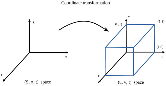
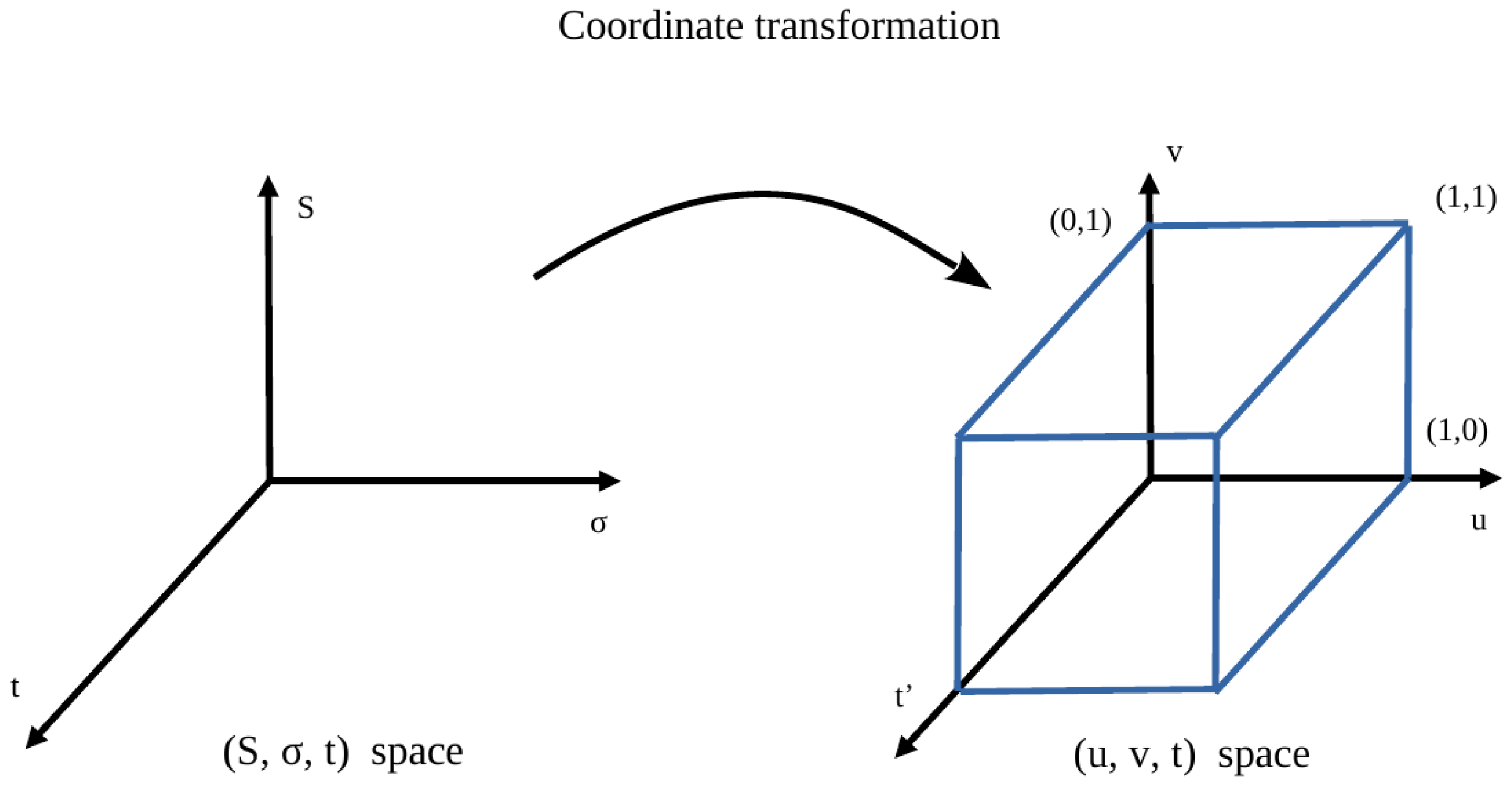
To do that, we need to perform the following change of variables from the initial space $(S,\sigma ,t)$ to the final space $(u,v,t^{\prime })$, where

$$u=\varphi (S,t),v=\psi (\sigma ,t)t^{\prime }=t$$

(24)

with the inverses

$$\begin{array}{cc}\hfill & S={\varphi }^{-1}(u,t^{\prime })\hfill \\ \hfill & \sigma ={\psi }^{-1}(v,t^{\prime })\hfill \end{array}$$

(25)

Note that the variables u and v, as defined by Equation (24), take values within the square $[0,1]\times [0,1]$ (see Figure 1). Consequently, the copula–Fokker–Planck equation is formulated on the unit square, and appropriate boundary conditions must be specified for this compact domain.

Figure 1. The figure depicts the transformation (24) that maps the complete space $(S,\sigma ,t)$ onto the unit square parallelepiped $(u,v,t^{\prime })$.

Thus, we can state the following theorem.

Theorem 1.

The Fokker–Planck equation for the copula density $c(u,v)$ is given by

$$\begin{array}{cc}\hfill {\displaystyle \frac{\partial c}{\partial t}}=& {\displaystyle \frac{1}{2}}{G}^2{f}^2(S,t){\displaystyle \frac{{\partial }^{2}c}{\partial u^2}}+{\displaystyle \frac{1}{2}}{q}^2{f}^2(\sigma ,t){\displaystyle \frac{{\partial }^{2}c}{\partial v^2}}+\rho Gqf(S,t)f(\sigma ,t){\displaystyle \frac{{\partial }^{2}c}{\partial u\partial v}}\hfill \\ \hfill & +\left[{\displaystyle \frac{1}{2}}{G}^{2}3{\displaystyle \frac{\partial }{\partial u}}\left[{\displaystyle \frac{f^2(S,t)}{2}}\right]+\rho Gq{\displaystyle \frac{f(S,t)}{f(\sigma ,t)}}{\displaystyle \frac{\partial }{\partial v}}\left[{\displaystyle \frac{f^2(\sigma ,t)}{2}}\right]-A_{S}f(S,t)-{\displaystyle \frac{\partial \varphi }{\partial t}}\right]\left({\displaystyle \frac{\partial c}{\partial u}}\right)\hfill \\ \hfill & +\left[{\displaystyle \frac{1}{2}}{q}^{2}3{\displaystyle \frac{\partial }{\partial v}}\left[{\displaystyle \frac{f^2(\sigma ,t)}{2}}\right]+\rho Gq{\displaystyle \frac{f(\sigma ,t)}{f(S,t)}}{\displaystyle \frac{\partial }{\partial u}}\left[{\displaystyle \frac{f^2(S,t)}{2}}\right]-A_{\sigma }f(\sigma ,t)-{\displaystyle \frac{\partial \psi }{\partial t}}\right]\left({\displaystyle \frac{\partial c}{\partial v}}\right)\hfill \\ \hfill & +\left[{\displaystyle \frac{\partial \varphi }{\partial t}}{\displaystyle \frac{-1}{f(S,t)}}{\displaystyle \frac{\partial f(S,t)}{\partial u}}+{\displaystyle \frac{\partial \psi }{\partial t}}{\displaystyle \frac{-1}{f(\sigma ,t)}}{\displaystyle \frac{\partial f(\sigma ,t)}{\partial v}}+{\displaystyle \frac{-1}{f(S,t)}}{\displaystyle \frac{\partial f(S,t)}{\partial t}}+{\displaystyle \frac{-1}{f(\sigma ,t)}}{\displaystyle \frac{\partial f(\sigma ,t)}{\partial t}}\right]c\hfill \\ \hfill & +\left[{\displaystyle \frac{1}{2}}{G}^2{\displaystyle \frac{{\partial }^2}{\partial u^2}}\left({\displaystyle \frac{f^2(S,t)}{2}}\right)+{\displaystyle \frac{1}{2}}{q}^2{\displaystyle \frac{{\partial }^2}{\partial v^2}}\left({\displaystyle \frac{f^2(\sigma ,t)}{2}}\right)+\rho Gq{\displaystyle \frac{\partial }{\partial u}}\left({\displaystyle \frac{f^2(S,t)}{2}}\right){\displaystyle \frac{\partial }{\partial v}}\left({\displaystyle \frac{f^2(\sigma ,t)}{2}}\right)\right]c\hfill \\ \hfill & +\left[-A_S{\displaystyle \frac{1}{f(S,t)}}{\displaystyle \frac{\partial }{\partial u}}\left[{\displaystyle \frac{f^2(S,t)}{2}}\right]-A_{\sigma }{\displaystyle \frac{1}{f(\sigma ,t)}}{\displaystyle \frac{\partial }{\partial v}}\left[{\displaystyle \frac{f^2(\sigma ,t)}{2}}\right]+\Phi \right]c\hfill \end{array}$$

(26)

We call to the above equation the copula–Fokker–Planck equation, where S and σ are given in terms of u and v by Equation (25) for $t^{\prime }=t$.

Proof. 

Consider the following change of variables (24) from the initial space $(S,\sigma ,t)$ to the final space $(u,v,t^{\prime })$, so that the partial derivatives in both spaces are related by

$${\displaystyle \frac{\partial }{\partial S}}={\displaystyle \frac{\partial }{\partial u}}{\displaystyle \frac{\partial u}{\partial S}}+{\displaystyle \frac{\partial }{\partial v}}{\displaystyle \frac{\partial v}{\partial S}}+{\displaystyle \frac{\partial }{\partial t^{\prime }}}{\displaystyle \frac{\partial t^{\prime }}{\partial S}}$$

(27)

$${\displaystyle \frac{\partial }{\partial \sigma }}={\displaystyle \frac{\partial }{\partial u}}{\displaystyle \frac{\partial u}{\partial \sigma }}+{\displaystyle \frac{\partial }{\partial v}}{\displaystyle \frac{\partial v}{\partial \sigma }}+{\displaystyle \frac{\partial }{\partial t^{\prime }}}{\displaystyle \frac{\partial t^{\prime }}{\partial \sigma }}$$

(28)

$${\displaystyle \frac{\partial }{\partial t}}={\displaystyle \frac{\partial }{\partial u}}{\displaystyle \frac{\partial u}{\partial t}}+{\displaystyle \frac{\partial }{\partial v}}{\displaystyle \frac{\partial v}{\partial t}}+{\displaystyle \frac{\partial }{\partial t^{\prime }}}{\displaystyle \frac{\partial t^{\prime }}{\partial t}}$$

(29)

or explicitly

$${\displaystyle \frac{\partial }{\partial S}}=\left({\displaystyle \frac{\partial \varphi }{\partial S}}\right){\displaystyle \frac{\partial }{\partial u}}=f(S,t){\displaystyle \frac{\partial }{\partial u}}$$

(30)

$${\displaystyle \frac{\partial }{\partial \sigma }}=\left({\displaystyle \frac{\partial \varphi }{\partial \sigma }}\right){\displaystyle \frac{\partial }{\partial v}}=f(\sigma ,t){\displaystyle \frac{\partial }{\partial v}}$$

(31)

$${\displaystyle \frac{\partial }{\partial t}}=\left({\displaystyle \frac{\partial \varphi }{\partial t}}\right){\displaystyle \frac{\partial }{\partial u}}+\left({\displaystyle \frac{\partial \psi }{\partial t}}\right){\displaystyle \frac{\partial }{\partial v}}+{\displaystyle \frac{\partial }{\partial t^{\prime }}}$$

(32)

and S and $\sigma$ can be written in terms of u and v (for each time instant $t^{\prime }$) trough its inverses (25).

The transformation (24) and the relations (30), (31), and (32) permit transforming the partial derivatives from the initial $(S,\sigma ,t)$ space to the $(u,v,t)$ space, where the copula density is defined. The continuation of the proof requires lengthy, tedious calculations, which are presented in Appendix A for the interested reader. □

According to copula theory, the copula distribution C (and consequently the copula density c) is independent of the marginal distributions. In contrast, the joint distribution P (along with its probability density p) exhibits an explicit dependency on the marginal distributions, as one can see in Equation (17).

Interestingly, when considering the Fokker–Planck equation, the probability density p in Equation (6) does not show an explicit dependence on the marginal distributions. However, the copula density c does have an explicit dependency on the marginals, as indicated by Equation (26).

The copula density c can be considered as an independent entity, separate from the marginal distributions, by inverting the conventional perspective and introducing specific functions (the bar-functions)

$$\overline{G}(u,v,t)=G(S,\sigma ,t)f(S,t)\overline{q}(u,v,t)=q(S,\sigma ,t)f(\sigma ,t)$$

(33)

Here, S and $\sigma$ on the right-hand side must be evaluated as functions of $(u,v,t)$ using the inverse relation (25). Additionally, new potentials ${\overline{A}}_u(u,v,t)$, ${\overline{A}}_v(u,v,t)$, and $\overline{\Phi }(u,v,t)$ are required. In terms of these new functions, the copula–Fokker–Planck equation is presented in the following theorem.

Theorem 2.

The copula–Fokker–Planck equation can be written as

$${\displaystyle \frac{\partial c}{\partial t}}={\displaystyle \frac{1}{2}}{\overline{G}}^2{\displaystyle \frac{{\partial }^{2}c}{\partial u^2}}+{\displaystyle \frac{1}{2}}{\overline{q}}^2{\displaystyle \frac{{\partial }^{2}c}{\partial v^2}}+\rho \overline{G}\overline{q}{\displaystyle \frac{{\partial }^{2}c}{\partial u\partial v}}-{\overline{A}}_u{\displaystyle \frac{\partial c}{\partial u}}-{\overline{A}}_v{\displaystyle \frac{\partial c}{\partial v}}+\overline{\Phi }c$$

(34)

where $\overline{G}$, $\overline{q}$, ${\overline{A}}_u$, ${\overline{A}}_v$ and $\overline{\Phi }$ are functions of the $(u,v,t)$ space that defines de dynamics of the copula density. These functions are related to G, q, $A_u$, $A_v$ and Φ functions on the $(S,\sigma ,t)$ space of Fokker–Planck Equation (6) for the probability density, according to

$$\overline{G}(u,v,t)=G(S,\sigma ,t)f(S,t)\overline{q}(u,v,t)=q(S,\sigma ,t)f(\sigma ,t)$$

(35)

$$-{\overline{A}}_u(u,v,t)={\displaystyle \frac{3}{2}}{\overline{G}}^2{\displaystyle \frac{\partial }{\partial u}}\left[lnf(S,t)\right]+\rho \overline{G}\overline{q}{\displaystyle \frac{\partial }{\partial v}}\left[lnf(\sigma ,t)\right]-A_{S}f(S,t)-{\displaystyle \frac{\partial \varphi }{\partial t}}$$

(36)

$$-{\overline{A}}_v(u,v,t)={\displaystyle \frac{3}{2}}{\overline{q}}^2{\displaystyle \frac{\partial }{\partial v}}\left[lnf(\sigma ,t)\right]+\rho \overline{G}\overline{q}{\displaystyle \frac{\partial }{\partial u}}\left[lnf(S,t)\right]-A_{\sigma }f(\sigma ,t)-{\displaystyle \frac{\partial \psi }{\partial t}}$$

(37)

$$\begin{array}{cc}\hfill \overline{\Phi }(u,v,t)=& -{\displaystyle \frac{\partial \varphi }{\partial t}}{\displaystyle \frac{\partial }{\partial u}}\left[lnf(S,t)\right]-{\displaystyle \frac{\partial \psi }{\partial t}}{\displaystyle \frac{\partial }{\partial v}}\left[lnf(\sigma ,t)\right]-{\displaystyle \frac{\partial }{\partial t}}\left[lnf(S,t)f(\sigma ,t)\right]\hfill \\ & +{\displaystyle \frac{1}{2}}{\displaystyle \frac{{\overline{G}}^2}{f^2(S,t)}}{\displaystyle \frac{{\partial }^2}{\partial u^2}}\left({\displaystyle \frac{f^2(S,t)}{2}}\right)+{\displaystyle \frac{1}{2}}{\displaystyle \frac{{\overline{q}}^2}{f^2(\sigma ,t)}}{\displaystyle \frac{{\partial }^2}{\partial v^2}}\left({\displaystyle \frac{f^2(\sigma ,t)}{2}}\right)\hfill \\ & +{\displaystyle \frac{\rho \overline{G}\overline{q}}{f(S,t)f(\sigma ,t)}}{\displaystyle \frac{\partial }{\partial u}}\left[{\displaystyle \frac{f^2(S,t)}{2}}\right]{\displaystyle \frac{\partial }{\partial v}}\left[{\displaystyle \frac{f^2(\sigma ,t)}{2}}\right]\hfill \\ & -A_S{\displaystyle \frac{1}{f(S,t)}}{\displaystyle \frac{\partial }{\partial u}}\left[{\displaystyle \frac{f^2(S,t)}{2}}\right]-A_{\sigma }{\displaystyle \frac{1}{f(\sigma ,t)}}{\displaystyle \frac{\partial }{\partial v}}\left[{\displaystyle \frac{f^2(\sigma ,t)}{2}}\right]+\Phi \hfill \end{array}$$

(38)

where the right sides of the above equations must be evaluated as functions of $(u,v,t)$ through Equation (25).

Proof. 

Consider Equation (26). In terms of $\overline{G}(u,v,t)=G(S,\sigma ,t)f(S,t)$ and $\overline{q}(u,v,t)=q(S,\sigma ,t)f(\sigma ,t)$ one can write

$$\begin{array}{cc}\hfill {\displaystyle \frac{\partial c}{\partial t}}=& {\displaystyle \frac{1}{2}}{\overline{G}}^2{\displaystyle \frac{{\partial }^{2}c}{\partial u^2}}+{\displaystyle \frac{1}{2}}{\overline{q}}^2{\displaystyle \frac{{\partial }^{2}c}{\partial v^2}}+\rho \overline{G}\overline{q}{\displaystyle \frac{{\partial }^{2}c}{\partial u\partial v}}\hfill \\ \hfill & +\left[{\displaystyle \frac{3}{2}}{\displaystyle \frac{{\overline{G}}^2}{f^2(S,t)}}{\displaystyle \frac{\partial }{\partial u}}\left[{\displaystyle \frac{f^2(S,t)}{2}}\right]+\rho {\displaystyle \frac{\overline{G}\overline{q}}{f^2(\sigma ,t)}}{\displaystyle \frac{\partial }{\partial v}}\left[{\displaystyle \frac{f^2(\sigma ,t)}{2}}\right]-A_{S}f(S,t)-{\displaystyle \frac{\partial \varphi }{\partial t}}\right]{\displaystyle \frac{\partial c}{\partial u}}\hfill \\ \hfill & +\left[{\displaystyle \frac{3}{2}}{\displaystyle \frac{{\overline{q}}^2}{f^2(\sigma ,t)}}{\displaystyle \frac{\partial }{\partial v}}\left[{\displaystyle \frac{f^2(\sigma ,t)}{2}}\right]+\rho {\displaystyle \frac{\overline{G}\overline{q}}{f^2(S,t)}}{\displaystyle \frac{\partial }{\partial u}}\left[{\displaystyle \frac{f^2(S,t)}{2}}\right]-A_{\sigma }f(\sigma ,t)-{\displaystyle \frac{\partial \psi }{\partial t}}\right]{\displaystyle \frac{\partial c}{\partial v}}\hfill \\ \hfill & +\left[-{\displaystyle \frac{\partial \varphi }{\partial t}}{\displaystyle \frac{1}{f(S,t)}}{\displaystyle \frac{\partial f(S,t)}{\partial u}}-{\displaystyle \frac{\partial \psi }{\partial t}}{\displaystyle \frac{1}{f(\sigma ,v)}}{\displaystyle \frac{\partial f(\sigma ,t)}{\partial v}}-{\displaystyle \frac{1}{f(S,t)}}{\displaystyle \frac{\partial f(S,t)}{\partial t}}-{\displaystyle \frac{1}{f(\sigma ,t)}}{\displaystyle \frac{\partial f(\sigma ,t)}{\partial t}}\right]c\hfill \\ \hfill & +\left[{\displaystyle \frac{1}{2}}{\displaystyle \frac{{\overline{G}}^2}{f^2(S,t)}}{\displaystyle \frac{{\partial }^2}{\partial u^2}}\left({\displaystyle \frac{f^2(S,t)}{2}}\right)+{\displaystyle \frac{1}{2}}{\displaystyle \frac{{\overline{q}}^2}{f^2(\sigma ,t)}}{\displaystyle \frac{{\partial }^2}{\partial v^2}}\left({\displaystyle \frac{f^2(\sigma ,t)}{2}}\right)\right]c\hfill \\ \hfill & +\left[{\displaystyle \frac{\rho \overline{G}\overline{q}}{f(S,t)f(\sigma ,t)}}{\displaystyle \frac{\partial }{\partial u}}\left({\displaystyle \frac{f^2(S,t)}{2}}\right){\displaystyle \frac{\partial }{\partial v}}\left({\displaystyle \frac{f^2(\sigma ,t)}{2}}\right)\right]c\hfill \\ \hfill & +\left[-A_S{\displaystyle \frac{1}{f(S,t)}}{\displaystyle \frac{\partial }{\partial u}}\left[{\displaystyle \frac{f^2(S,t)}{2}}\right]-A_{\sigma }{\displaystyle \frac{1}{f(\sigma ,t)}}{\displaystyle \frac{\partial }{\partial v}}\left[{\displaystyle \frac{f^2(\sigma ,t)}{2}}\right]+\Phi \right]c\hfill \end{array}$$

(39)

Now by defining the magnetic and electric bar potentials ${\overline{A}}_u$, ${\overline{A}}_v$ and $\overline{\Phi }$ as

$$-{\overline{A}}_u(u,v,t)={\displaystyle \frac{3}{2}}{\overline{G}}^2{\displaystyle \frac{\partial }{\partial u}}\left[lnf(S,t)\right]+\rho \overline{G}\overline{q}{\displaystyle \frac{\partial }{\partial v}}\left[lnf(\sigma ,t)\right]-A_{S}f(S,t)-{\displaystyle \frac{\partial \varphi }{\partial t}}$$

(40)

$$-{\overline{A}}_v(u,v,t)={\displaystyle \frac{3}{2}}{\overline{q}}^2{\displaystyle \frac{\partial }{\partial v}}\left[lnf(\sigma ,t)\right]+\rho \overline{G}\overline{q}{\displaystyle \frac{\partial }{\partial u}}\left[lnf(S,t)\right]-A_{\sigma }f(\sigma ,t)-{\displaystyle \frac{\partial \psi }{\partial t}}$$

(41)

$$\begin{array}{cc}\hfill \overline{\Phi }(u,v,t)=& -{\displaystyle \frac{\partial \varphi }{\partial t}}{\displaystyle \frac{\partial }{\partial u}}\left[lnf(S,t)\right]-{\displaystyle \frac{\partial \psi }{\partial t}}{\displaystyle \frac{\partial }{\partial v}}\left[lnf(\sigma ,t)\right]-{\displaystyle \frac{\partial }{\partial t}}\left[lnf(S,t)f(\sigma ,t)\right]\hfill \\ & +{\displaystyle \frac{1}{2}}{\displaystyle \frac{{\overline{G}}^2}{f^2(S,t)}}{\displaystyle \frac{{\partial }^2}{\partial u^2}}\left({\displaystyle \frac{f^2(S,t)}{2}}\right)+{\displaystyle \frac{1}{2}}{\displaystyle \frac{{\overline{q}}^2}{f^2(\sigma ,t)}}{\displaystyle \frac{{\partial }^2}{\partial v^2}}\left({\displaystyle \frac{f^2(\sigma ,t)}{2}}\right)\hfill \\ & +{\displaystyle \frac{\rho \overline{G}\overline{q}}{f(S,t)f(\sigma ,t)}}{\displaystyle \frac{\partial }{\partial u}}\left[{\displaystyle \frac{f^2(S,t)}{2}}\right]{\displaystyle \frac{\partial }{\partial v}}\left[{\displaystyle \frac{f^2(\sigma ,t)}{2}}\right]\hfill \\ & -A_S{\displaystyle \frac{1}{f(S,t)}}{\displaystyle \frac{\partial }{\partial u}}\left[{\displaystyle \frac{f^2(S,t)}{2}}\right]-A_{\sigma }{\displaystyle \frac{1}{f(\sigma ,t)}}{\displaystyle \frac{\partial }{\partial v}}\left[{\displaystyle \frac{f^2(\sigma ,t)}{2}}\right]+\Phi \hfill \end{array}$$

(42)

the copula–Fokker–Planck equation becomes

$${\displaystyle \frac{\partial c}{\partial t}}={\displaystyle \frac{1}{2}}{\overline{G}}^2{\displaystyle \frac{{\partial }^{2}c}{\partial u^2}}+{\displaystyle \frac{1}{2}}{\overline{q}}^2{\displaystyle \frac{{\partial }^{2}c}{\partial v^2}}+\rho \overline{G}\overline{q}{\displaystyle \frac{{\partial }^{2}c}{\partial u\partial v}}-{\overline{A}}_u{\displaystyle \frac{\partial c}{\partial u}}-{\overline{A}}_v{\displaystyle \frac{\partial c}{\partial v}}+\overline{\Phi }c$$

□

In the last equation $\overline{G}$, $\overline{q}$, ${\overline{A}}_u$, ${\overline{A}}_v$ and $\overline{\Phi }$ are a set of given functions that determine the dynamics of the copula density independently of the probability density p.

Interpretation

To give an interpretation of the copula–Fokker–Planck equation, one can ask if there exists a stochastic system for the u and v variables, so one recovers Equation (34) via Equations (2), (3), and (6). That is, what are the corresponding drifts?

To do that, one can consider the transformation (24). By the Ito’s lemma, one has then that

$$du={\displaystyle \frac{\partial \varphi }{\partial t}}dt+{\displaystyle \frac{\partial \varphi }{\partial S}}dS+{\displaystyle \frac{1}{2}}{\displaystyle \frac{{\partial }^2\varphi }{\partial S^2}}d{S}^2$$

(43)

$$dv={\displaystyle \frac{\partial \psi }{\partial t}}dt+{\displaystyle \frac{\partial \psi }{\partial \sigma }}d\sigma +{\displaystyle \frac{1}{2}}{\displaystyle \frac{{\partial }^2\psi }{\partial {\sigma }^2}}d{\sigma }^2$$

(44)

Using (2), (3), (15), and (16) gives

$$du=\left({\displaystyle \frac{\partial \varphi }{\partial t}}+f(S,t)\mu +{\displaystyle \frac{1}{2}}{\displaystyle \frac{\partial f(S,t)}{\partial S}}\right)dt+f(S,t)Gd{W}_S$$

$$dv=\left({\displaystyle \frac{\partial \psi }{\partial t}}+f(\sigma ,t)r+{\displaystyle \frac{1}{2}}{\displaystyle \frac{\partial f(\sigma ,t)}{\partial \sigma }}\right)dt+f(\sigma ,t)qd{W}_{\sigma }$$

or

$$du=\left({\displaystyle \frac{\partial \varphi }{\partial t}}+f(S,t)\mu +{\displaystyle \frac{1}{4}}{\displaystyle \frac{\partial f{(S,t)}^2}{\partial u}}\right)dt+f(S,t)Gd{W}_S={\mu }_{u}dt+f(S,t)Gd{W}_S$$

(45)

$$dv=\left({\displaystyle \frac{\partial \psi }{\partial t}}+f(\sigma ,t)r+{\displaystyle \frac{1}{4}}{\displaystyle \frac{\partial f{(\sigma ,t)}^2}{\partial v}}\right)dt+f(\sigma ,t)qd{W}_{\sigma }={\mu }_{v}dt+f(\sigma ,t)qd{W}_{\sigma }$$

(46)

where S and $\sigma$ are thought of as functions of u and v through Equation (25). Let $D(u,v)$ be the probability density for the u and v variables, so by analogy with (2), (3) and (6), one can show that $D(u,v)$ satisfies the equation

$$\begin{array}{cc}\hfill {\displaystyle \frac{\partial D}{\partial t}}=& {\displaystyle \frac{1}{2}}{G}^2{f}^2(S,t){\displaystyle \frac{{\partial }^{2}D}{\partial u^2}}+{\displaystyle \frac{1}{2}}{q}^2{f}^2(\sigma ,t){\displaystyle \frac{{\partial }^{2}D}{\partial v^2}}+\rho Gqf(S,t)f(\sigma ,t){\displaystyle \frac{{\partial }^{2}D}{\partial u\partial v}}\hfill \\ \hfill & +\left[{\displaystyle \frac{1}{2}}{G}^{2}3{\displaystyle \frac{\partial }{\partial u}}\left[{\displaystyle \frac{f^2(S,t)}{2}}\right]+\rho Gq{\displaystyle \frac{f(S,t)}{f(\sigma ,t)}}{\displaystyle \frac{\partial }{\partial v}}\left[{\displaystyle \frac{f^2(\sigma ,t)}{2}}\right]-A_{S}f(S,t)-{\displaystyle \frac{\partial \varphi }{\partial t}}\right]\left({\displaystyle \frac{\partial D}{\partial u}}\right)\hfill \\ \hfill & +\left[{\displaystyle \frac{1}{2}}{q}^{2}3{\displaystyle \frac{\partial }{\partial v}}\left[{\displaystyle \frac{f^2(\sigma ,t)}{2}}\right]+\rho Gq{\displaystyle \frac{f(\sigma ,t)}{f(S,t)}}{\displaystyle \frac{\partial }{\partial u}}\left[{\displaystyle \frac{f^2(S,t)}{2}}\right]-A_{\sigma }f(\sigma ,t)-{\displaystyle \frac{\partial \psi }{\partial t}}\right]\left({\displaystyle \frac{\partial D}{\partial v}}\right)\hfill \\ \hfill & +\mathcal{U}D\hfill \end{array}$$

(47)

The above equation is closely related to the copula–Fokker–Planck Equation (26). In fact, $\overline{\Phi }=\mathcal{U}+\mathrm{extra}\mathrm{terms}$. Thus, the copula–Fokker–Planck Equation (26) is not just the Fokker–Planck equation associated with the stochastic system (45) and (46), but a modified version of it, which differs in Electric potential terms. Still, drifts can be identified as the temporal part of the stochastic equations, that is,

$${\mu }_u=\left({\displaystyle \frac{\partial \varphi }{\partial t}}+f(S,t)\mu +{\displaystyle \frac{1}{4}}{\displaystyle \frac{\partial f{(S,t)}^2}{\partial u}}\right)$$

$${\mu }_v=\left({\displaystyle \frac{\partial \psi }{\partial t}}+f(\sigma ,t)r+{\displaystyle \frac{1}{4}}{\displaystyle \frac{\partial f{(\sigma ,t)}^2}{\partial v}}\right)$$

Note that drifts do not depend on the correlation parameter $\rho$.

If there exists a stochastic differential system of the form

$$du={\alpha }_u(u,v)dt+{\beta }_u(u,v)d{W}_S$$

$$dv={\alpha }_v(u,v)dt+{\beta }_v(u,v)d{W}_{\sigma }$$

from which one can deduce the copula–Fokker–Planck Equation (26) remains an open question. A comprehensive analysis of these issues and their equivalences exceeds the scope of this paper and will be addressed in future research.

As an example, consider the Fokker–Planck Equation (6) for the time-independent case (${\displaystyle \frac{\partial P}{\partial t}}=0$) and take $G=1$, $q=1$, $\mu =-{\displaystyle \frac{S}{{\sigma }_0^2}}$ and $r=-{\displaystyle \frac{\sigma }{{\sigma }_0^2}}$. This imply that $A_S={\displaystyle \frac{S}{{\sigma }_0^2}}$, $A_{\sigma }={\displaystyle \frac{\sigma }{{\sigma }_0^2}}$ and $\Phi ={\displaystyle \frac{2}{{\sigma }_0^2}}$, so the Fokker–Planck equation is

$$0={\displaystyle \frac{1}{2}}{\displaystyle \frac{{\partial }^{2}p}{\partial S^2}}+\rho {\displaystyle \frac{{\partial }^{2}p}{\partial S\partial \sigma }}+{\displaystyle \frac{1}{2}}{\displaystyle \frac{{\partial }^{2}p}{\partial {\sigma }^2}}+{\displaystyle \frac{S}{{\sigma }_0^2}}{\displaystyle \frac{\partial p}{\partial S}}+{\displaystyle \frac{\sigma }{{\sigma }_0^2}}{\displaystyle \frac{\partial p}{\partial \sigma }}+{\displaystyle \frac{2}{{\sigma }_0^2}}$$

(48)

The standard solution of the above equation is the bivariate normal density

$$p(S,\sigma )={\displaystyle \frac{e^{\left(-\frac{1}{2{\sigma }_0^2}\left(S\sigma \right){\rho }^{-1}{\left(S\sigma \right)}^{\mathrm{T}}\right)}}{\sqrt{{\left(2\pi \right)}^2{\sigma }_0^4\left|\rho \right|}}}$$

where $\rho$ is the correlation matrix. The corresponding time-independent marginal densities are in this case

$$f\left(S\right)={\displaystyle \frac{1}{\sqrt{2\pi {\sigma }_0^2}}}{e}^{-{\displaystyle \frac{S^2}{2{\sigma }_0^2}}}f\left(\sigma \right)={\displaystyle \frac{1}{\sqrt{2\pi {\sigma }_0^2}}}{e}^{-{\displaystyle \frac{{\sigma }^2}{2{\sigma }_0^2}}}$$

so the copula density given (21) is just

$$c(u,v)={\displaystyle \frac{p(S,\sigma )}{f\left(S\right)f\left(\sigma \right)}}=e^{{\displaystyle \frac{S^2}{2{\sigma }_0^2}}}{e}^{{\displaystyle \frac{{\sigma }^2}{2{\sigma }_0^2}}}{\displaystyle \frac{e^{\left(-\frac{1}{2{\sigma }_0^2}\left(S\sigma \right){\rho }^{-1}{\left(S\sigma \right)}^{\mathrm{T}}\right)}}{\sqrt{\left|\rho \right|}}}$$

or [7]

$$c(u,v)={\displaystyle \frac{e^{\left(-\frac{1}{2{\sigma }_0^2}\left(S\sigma \right)\left[{\rho }^{-1}-\mathit{I}\right]{\left(S\sigma \right)}^{\mathrm{T}}\right)}}{\sqrt{\left|\rho \right|}}}$$

(49)

where S and $\sigma$ are given in terms of u and v, respectively, according (25), that is

$$S=N_{{\sigma }_0}\left(u\right)\mathrm{and}\sigma =N_{{\sigma }_0}\left(\sigma \right)$$

(50)

with $N_{{\sigma }_0}$ the normal distribution function with mean zero and variance ${\sigma }_0$. The copula density (49), according to Theorem 2, is the solution to the following time-independent copula–Fokker–Planck equation

$$\begin{array}{cc}\hfill 0=& {\displaystyle \frac{1}{2}}f\left(S\right){\displaystyle \frac{{\partial }^{2}c}{\partial u^2}}+{\displaystyle \frac{1}{2}}f{\left(\sigma \right)}^2{\displaystyle \frac{{\partial }^{2}c}{\partial v^2}}+\rho f\left(S\right)f\left(\sigma \right){\displaystyle \frac{{\partial }^{2}c}{\partial u\partial v}}\hfill \\ \hfill & -\left[{\displaystyle \frac{3}{2}}S+\rho \sigma \right]{\displaystyle \frac{f\left(S\right)}{{\sigma }_0^2}}{\displaystyle \frac{\partial c}{\partial u}}-\left[{\displaystyle \frac{3}{2}}\sigma +\rho S\right]{\displaystyle \frac{f\left(\sigma \right)}{{\sigma }_0^2}}{\displaystyle \frac{\partial c}{\partial u}}\hfill \\ \hfill & \left[{\displaystyle \frac{1}{2{\sigma }_0^2}}\left({\displaystyle \frac{S^2}{{\sigma }_0^2}}-1\right)+{\displaystyle \frac{1}{2{\sigma }_0^2}}\left({\displaystyle \frac{{\sigma }^2}{{\sigma }_0^2}}-1\right)+\rho f\left(S\right)f\left(\sigma \right){\displaystyle \frac{S\sigma }{{\sigma }_0^4}}\right]\hfill \end{array}$$

(51)

where again S and $\sigma$ are given by (50) in terms of u and v.

Also, one can ask: what is the Fokker–Planck for the probability density p in terms of the new copula functions $\overline{G}$, $\overline{q}$, ${\overline{A}}_u$, ${\overline{A}}_v$ and $\overline{\Phi }$? The following proposition gives the answer:

Collolary 1.

Given the copula–Fokker–Planck Equation (34) for the copula density c (defined by the bar functions $\overline{G}$, $\overline{q}$, ${\overline{A}}_u$, ${\overline{A}}_v$ and $\overline{\Phi }$) and two marginals densities $f(S,t)$ and $f(\sigma ,t)$ then, the Fokker–Planck equation for the probability density $p=p(S,\sigma ,t)=c\left[\varphi \right(S,t),\psi (\sigma ,t),t]f(S,t)f(\sigma ,t)$ is given by

$${\displaystyle \frac{\partial p}{\partial t}}={\displaystyle \frac{1}{2}}{G}^2{\displaystyle \frac{{\partial }^{2}p}{\partial S^2}}+\rho Gq{\displaystyle \frac{{\partial }^{2}p}{\partial S\partial \sigma }}+{\displaystyle \frac{1}{2}}{q}^2{\displaystyle \frac{{\partial }^{2}p}{\partial {\sigma }^2}}-A_S{\displaystyle \frac{\partial p}{\partial S}}-A_{\sigma }{\displaystyle \frac{\partial p}{\partial \sigma }}+\Phi p$$

(52)

where

$$G={\displaystyle \frac{\overline{G}}{f(S,t)}}$$

(53)

$$q={\displaystyle \frac{\overline{q}}{f(\sigma ,t)}}$$

(54)

$$A_S={\displaystyle \frac{1}{f(S,t)}}\left[{\overline{A}}_u+{\displaystyle \frac{3}{2}}{\overline{G}}^2{\displaystyle \frac{\partial }{\partial u}}\left[lnf(S,t)\right]+\rho \overline{G}\overline{q}{\displaystyle \frac{\partial }{\partial v}}\left[lnf(\sigma ,t)\right]-{\displaystyle \frac{\partial \varphi }{\partial t}}\right]$$

(55)

$$A_{\sigma }={\displaystyle \frac{1}{f(\sigma ,t)}}\left[{\overline{A}}_v+{\displaystyle \frac{3}{2}}{\overline{q}}^2{\displaystyle \frac{\partial }{\partial v}}\left[lnf(\sigma ,t)\right]+\rho \overline{G}\overline{q}{\displaystyle \frac{\partial }{\partial u}}\left[lnf(S,t)\right]-{\displaystyle \frac{\partial \psi }{\partial t}}\right]$$

(56)

and

$$\begin{array}{cc}\hfill \Phi =& \overline{\Phi }+{\overline{A}}_S{\displaystyle \frac{1}{f(S,t)}}{\displaystyle \frac{\partial }{\partial u}}\left[{\displaystyle \frac{f^2(S,t)}{2}}\right]-{\overline{A}}_{\sigma }{\displaystyle \frac{1}{f(\sigma ,t)}}{\displaystyle \frac{\partial }{\partial v}}\left[{\displaystyle \frac{f^2(\sigma ,t)}{2}}\right]\hfill \\ \hfill & -{\displaystyle \frac{\rho \overline{G}\overline{q}}{f(S,t)f(\sigma ,t)}}{\displaystyle \frac{\partial }{\partial u}}\left[{\displaystyle \frac{f^2(S,t)}{2}}\right]{\displaystyle \frac{\partial }{\partial v}}\left[{\displaystyle \frac{f^2(\sigma ,t)}{2}}\right]\hfill \\ \hfill & -{\displaystyle \frac{1}{2}}{\displaystyle \frac{{\overline{G}}^2}{f^2(S,t)}}{\displaystyle \frac{{\partial }^2}{\partial u^2}}\left({\displaystyle \frac{f^2(S,t)}{2}}\right)-{\displaystyle \frac{1}{2}}{\displaystyle \frac{{\overline{q}}^2}{f^2(\sigma ,t)}}{\displaystyle \frac{{\partial }^2}{\partial v^2}}\left({\displaystyle \frac{f^2(\sigma ,t)}{2}}\right)\hfill \\ \hfill & -{\displaystyle \frac{\partial \varphi }{\partial t}}{\displaystyle \frac{\partial }{\partial u}}\left[lnf(S,t)\right]-{\displaystyle \frac{\partial \psi }{\partial t}}{\displaystyle \frac{\partial }{\partial v}}\left[lnf(\sigma ,t)\right]-{\displaystyle \frac{\partial }{\partial t}}\left[lnf(S,t)f(\sigma ,t)\right]\hfill \end{array}$$

(57)

Proof. 

The proof consist in to invert the functions G, q, $A_u$, $A_v$ and $\Phi$ in terms of $\overline{G}$, $\overline{q}$, ${\overline{A}}_u$, ${\overline{A}}_v$ and $\overline{\Phi }$ by using Equations (35)–(38). In an explicit form, the potentials are

$$A_S={\displaystyle \frac{1}{f(S,t)}}\left[{\overline{A}}_u+{\displaystyle \frac{3}{2}}{\overline{G}}^2{\displaystyle \frac{1}{f(S,t)}}{\displaystyle \frac{\partial }{\partial S}}\left[lnf(S,t)\right]+\rho \overline{G}\overline{q}{\displaystyle \frac{1}{f(\sigma ,t)}}{\displaystyle \frac{\partial }{\partial \sigma }}\left[lnf(\sigma ,t)\right]-{\displaystyle \frac{\partial \varphi }{\partial t}}\right]$$

(58)

$$A_{\sigma }={\displaystyle \frac{1}{f(\sigma ,t)}}\left[{\overline{A}}_v+{\displaystyle \frac{3}{2}}{\overline{q}}^2{\displaystyle \frac{1}{f(\sigma ,t)}}{\displaystyle \frac{\partial }{\partial \sigma }}\left[lnf(\sigma ,t)\right]+\rho \overline{G}\overline{q}{\displaystyle \frac{\partial }{\partial S}}{\displaystyle \frac{1}{f(S,t)}}\left[lnf(S,t)\right]-{\displaystyle \frac{\partial \psi }{\partial t}}\right]$$

(59)

and

$$\begin{array}{cc}\hfill \Phi =& \overline{\Phi }+{\overline{A}}_S{\displaystyle \frac{\partial }{\partial S}}\left[lnf(S,t)\right]-{\overline{A}}_{\sigma }{\displaystyle \frac{\partial }{\partial \sigma }}\left[lnf(\sigma ,t)\right]\hfill \\ \hfill & -\rho \overline{G}\overline{q}{\displaystyle \frac{\partial }{\partial S}}\left[lnf(S,t)\right]{\displaystyle \frac{\partial }{\partial \sigma }}\left[lnf(\sigma ,t)\right]\hfill \\ \hfill & -{\displaystyle \frac{1}{2}}{\displaystyle \frac{{\overline{G}}^2}{f^3(S,t)}}{\displaystyle \frac{{\partial }^{2}f(S,t)}{\partial S^2}}-{\displaystyle \frac{1}{2}}{\displaystyle \frac{{\overline{q}}^2}{f^3(\sigma ,t)}}{\displaystyle \frac{{\partial }^{2}f(\sigma ,t)}{\partial {\sigma }^2}}\hfill \\ \hfill & -{\displaystyle \frac{\partial \varphi }{\partial t}}{\displaystyle \frac{1}{f^2(S,t)}}{\displaystyle \frac{\partial f(S,t)}{\partial S}}-{\displaystyle \frac{\partial \psi }{\partial t}}{\displaystyle \frac{1}{f^2(\sigma ,t)}}{\displaystyle \frac{\partial f(\sigma ,t)}{\partial \sigma }}-{\displaystyle \frac{\partial }{\partial t}}\left[lnf(S,t)f(\sigma ,t)\right]\hfill \end{array}$$

(60)

□

In the last equations, one can see explicitly the contributions of the marginals to the probability density p. To determine p one can solve (52) directly, or one can to integrate (34) to obtain c first. Given the two marginal densities $f(S,t)$ and $f(\sigma ,t)$, one can obtain p by using Equation (21).

From an applied financial perspective, the main advantage of the present formulation is that it separates, at the operator level, the dynamics governing marginal volatility behaviour from those governing dependence. In standard multivariate stochastic-volatility models, changes in cross-asset dependence are often calibrated jointly with the parameters controlling the marginal volatility processes, which can make interpretation and stress analysis difficult. By contrast, the copula–Fokker–Planck representation developed here allows one to study how the dependence structure evolves over time without rewriting the entire marginal specification. This is potentially useful in applications where one wishes to alter or stress the dependence pattern while preserving the individual marginal dynamics, for example, in risk management, scenario analysis, or the study of time-varying contagion. Even when no closed-form solution is available, the framework provides a systematic analytical decomposition that may support future calibration schemes and numerical implementations for stochastic-volatility models with non-Gaussian dependence.

5. Distribution Copula Boundary Conditions

In this section, we analize some conditions for the copula distribution which will permit us to obtain a unique copula distribution from the copula density $c(u,v,t)$. As is well known in the literature for the time-independent case [7,14,45,55] a copula distribution $C(u,v)$ satisfies the conditions

$$C\left(u_2,v_2\right)+C\left(u_1,v_1\right)-C\left(u_2,v_1\right)-C\left(u_1,v_2\right)\ge 0$$

(61)

for $0\le u_1\le u_2\le 1,0\le v_1\le v_2\le 1$, and

$$C(u,1)=uC(u,0)=0,\forall u\in [0,1],$$

(62)

$$C(1,v)=vC(0,v)=0,\forall v\in [0,1]$$

(63)

Some consequences of (61) $\forall u,v\in [0,1]$, are:

$$c(u,v)\ge 00\le {\displaystyle \frac{\partial C(u,v)}{\partial u}}\le 10\le {\displaystyle \frac{\partial C(u,v)}{\partial v}}\le 1$$

(64)

This follows from the fact that a copula, being a distribution function, is non-decreasing in both variables. Therefore, the difference quotients are non-negative. Furthermore, since a copula is also a Lipschitz function with Lipschitz coefficient 1, it follows that the derivatives are bounded by 1 [14,55].

For the time-dependent case, one can consider Equation (64) as equivalent to (61) in the case of the Fokker–Planck copula description. In fact, one would impose these conditions, along with Equations (62) and (63), on the copula distribution during the time evolution. In this way, we consider the following conditions for the copula distribution in the time-dependent case: if $t>0$ then

$$C(u,1,t)=uC(u,0,t)=0,\forall u\in [0,1],$$

(65)

$$C(1,v,t)=vC(0,v,t)=0,\forall v\in [0,1]$$

(66)

$$0\le {\displaystyle \frac{\partial C}{\partial u}}(u,v,t)\le 1,\forall u,v\in [0,1]$$

(67)

$$0\le {\displaystyle \frac{\partial C}{\partial v}}(u,v,t)\le 1,\forall u,v\in [0,1]$$

(68)

$$c(u,v,t)={\displaystyle \frac{{\partial }^{2}C}{\partial u\partial v}}\ge 0\forall u,v\in [0,1]$$

(69)

Note that for a given copula density $c(u,v,t)$, which is a solution of the copula–Fokker–Planck Equation (34), the copula distribution $C(u,v,t)$ in principle is not determined uniquely. The following theorem establishes that the solution is unique:

Theorem 3.

Let $C(u,v,t)$ and $C^{\prime }(u,v,t)$ two copulas distributions associated to the same copula density $c(u,v,t)$, that is

$$c(u,v,t)={\displaystyle \frac{{\partial }^{2}C(u,v,t)}{\partial u\partial v}}={\displaystyle \frac{{\partial }^2{C}^{\prime }(u,v,t)}{\partial u\partial v}}.$$

If $C$and $C^{\prime }$ satisfy the boundary conditions (65) to (69), then $C=C^{\prime }$.

Proof. 

As

$${\displaystyle \frac{{\partial }^{2}C(u,v,t)}{\partial u\partial v}}={\displaystyle \frac{{\partial }^2{C}^{\prime }(u,v,t)}{\partial u\partial v}}$$

then one can write

$$C^{\prime }(u,v,t)=C(u,v,t)+\varphi (u,t)+\chi (v,t)$$

But C must satisfy Equations (67) and (68) so

$$0\le {\displaystyle \frac{\partial C(u,v,t)}{\partial u}}\le 10\le {\displaystyle \frac{\partial C(u,v,t)}{\partial v}}\le 1$$

(70)

By adding ${\displaystyle \frac{\partial \varphi (u,t)}{\partial u}}$ and ${\displaystyle \frac{\partial \chi (v,t)}{\partial v}}$ respectively, one has that

$${\displaystyle \frac{\partial \varphi (u,t)}{\partial u}}\le {\displaystyle \frac{\partial C(u,v,t)}{\partial u}}+{\displaystyle \frac{\partial \varphi (u,t)}{\partial u}}\le 1+{\displaystyle \frac{\partial \varphi (u,t)}{\partial u}}$$

(71)

$${\displaystyle \frac{\partial \chi (v,t)}{\partial v}}\le {\displaystyle \frac{\partial C(u,v,t)}{\partial v}}+{\displaystyle \frac{\partial \chi (v,t)}{\partial v}}\le 1+{\displaystyle \frac{\partial \chi (v,t)}{\partial v}}$$

(72)

But also $C^{\prime }$ satisfy (67) and (68), thus

$$0\le {\displaystyle \frac{\partial C(u,v,t)}{\partial u}}+{\displaystyle \frac{\partial \varphi (u,t)}{\partial u}}\le 1$$

(73)

$$0\le {\displaystyle \frac{\partial C(u,v,t)}{\partial v}}+{\displaystyle \frac{\partial \chi (v,t)}{\partial v}}\le 1$$

(74)

By subtracting Equation (73) to (71) and (74) to (72) respectively, one has that

$${\displaystyle \frac{\partial \varphi (v,t)}{\partial u}}\le 0\le {\displaystyle \frac{\partial \varphi (u,t)}{\partial u}}$$

(75)

$${\displaystyle \frac{\partial \varphi (v,t)}{\partial u}}\le 0\le {\displaystyle \frac{\partial \varphi (u,t)}{\partial u}}$$

(76)

then

$$0\le {\displaystyle \frac{\partial \varphi (v,t)}{\partial u}}\le 0$$

(77)

$$0\le {\displaystyle \frac{\partial \chi (v,t)}{\partial v}}\le 0$$

(78)

thus

$${\displaystyle \frac{\partial \varphi (v,t)}{\partial u}}=0$$

(79)

$${\displaystyle \frac{\partial \chi (v,t)}{\partial v}}=0$$

(80)

so $\varphi (u,t)=\varphi \left(t\right)$ and $\chi (v,t)=\chi \left(t\right)$. In this way both copulas $C^{\prime }$ and C are related by

$$C^{\prime }(u,v,t)=C(u,v,t)+\varphi \left(t\right)+\chi \left(t\right)=C(u,v,t)+\gamma \left(t\right)$$

By evaluating the above equation in $v=0$

$$C^{\prime }(u,0,t)=C(u,0,t)+\gamma \left(t\right)$$

But Equation (65) implies that $\gamma \left(t\right)=0$ for all t. Thus $C^{\prime }=C$, and there is a unique copula distribution associated with the copula density c that satisfies the boundary conditions (65) to (69). □

In a forthcoming paper, we will discuss the boundary conditions for the copula density $c(u,v)$, but here we can give some initial comments. First, one can note that, through the inverse of Equation (20), that is

$$C(u,v,t)={\int }_0^u{\int }_0^{v}c\left(u^{\prime },v^{\prime },t\right)d{u}^{\prime }d{v}^{\prime }$$

(81)

the conditions (65) and (66) become integral equations for the copula density $c(u,v,t)$. Thus, the copula density must satisfy, as boundary conditions, the following integral equations

$$u=C(u,1,t)={\int }_0^u{\int }_0^{1}c\left(u^{\prime },v^{\prime },t\right)d{u}^{\prime }d{v}^{\prime }$$

(82)

$$v=C(1,v,t)={\int }_0^1{\int }_0^{v}c\left(u^{\prime },v^{\prime },t\right)d{u}^{\prime }d{v}^{\prime }$$

(83)

or by taking derivatives

$$1={\int }_0^{1}c\left(u,v^{\prime },t\right)d{v}^{\prime }$$

(84)

$$1={\int }_0^{1}c\left(u^{\prime },v,t\right)d{u}^{\prime }$$

(85)

Secondly, conditions (67) and (68) imply that the copula density must accomplish

$$0\le {\int }_0^{v}c\left(u,v^{\prime },t\right)d{v}^{\prime }\le 1\forall u\in [0,1]$$

(86)

and

$$0\le {\int }_0^{u}c\left(u^{\prime },v,t\right)d{u}^{\prime }\le 1\forall v\in [0,1]$$

(87)

From a partial differential equation perspective, the nature of these boundary conditions can be explicitly classified. Because the variables u and v are strictly confined to the compact domain $[0,1]\times [0,1]$, and the copula density $c(u,v,t)$ must perfectly conserve probability to satisfy the uniform marginal constraints in Equations (84) and (85), no probability mass can exit the unit square. Consequently, the boundaries of the copula–Fokker–Planck equation act as reflecting (no-flux) boundary conditions. In the physical terminology of the Fokker–Planck equation, this implies that the normal component of the probability current $\overrightarrow{J}$ must vanish at the boundaries ($u=0,1$ and $v=0,1$), ensuring that the system remains purely conservative.

These boundary conditions also admit a natural financial interpretation. Since the copula encodes the dependence structure separately from the marginal behaviour, the constraints in Equations (86) and (87) regulate how probability mass may be allocated over the unit square, especially near its boundaries and corners. In financial terms, this is directly related to the behaviour of asset returns under extreme market configurations. Concentration of mass near the lower-left or upper-right corners corresponds to stronger comovement in joint downturns or upturns, whereas weaker accumulation near the corners is consistent with more moderate tail interaction or asymptotic independence. From this perspective, the boundary conditions are not merely technical requirements for well-posedness and uniqueness; they also determine whether the admissible copula dynamics can represent forms of tail dependence that are relevant for systemic risk, contagion, and stress-testing exercises in stochastic-volatility environments.

6. The Uncorrelated Case $\mathit{\rho }=\mathbf{0}$

As a consistency and sanity check of the proposed framework, it is instructive to examine the uncorrelated case $(\rho =0)$. It is important to emphasize that within the context of the Fokker–Planck equation, a zero correlation parameter does not automatically imply that the associated copula reduces to the independence copula. Instead, the copula density achieves mathematical independence $\left(c(u,v,t)=c_1(u,t)c_2(v,t)\right)$ if and only if highly specific structural constraints regarding the effective potentials (conditions i, ii, and iii below) are satisfied. This demonstrates the framework’s capability to capture complex, non-linear dependencies that persist even when linear correlation vanishes.

Consider the Equation (34) when the Brownian motions in (4) are uncorrelated, that is, one has $\rho =0$ and Equation (34) becomes

$${\displaystyle \frac{\partial c}{\partial t}}={\displaystyle \frac{1}{2}}{\overline{G}}^2{\displaystyle \frac{{\partial }^{2}c}{\partial u^2}}+{\displaystyle \frac{1}{2}}{\overline{q}}^2{\displaystyle \frac{{\partial }^{2}c}{\partial v^2}}-{\overline{A}}_u{\displaystyle \frac{\partial c}{\partial u}}-{\overline{A}}_v{\displaystyle \frac{\partial c}{\partial v}}+\overline{\Phi }c$$

(88)

then, one can states the following proposition.

Proposition 1.

The value $\rho =0$ in the underlying diffusion Equation (88) does not, in general, imply an independent copula.

Proof. 

If the functions $\overline{G}$, $\overline{q}$, ${\overline{A}}_u$, ${\overline{A}}_v$, $\overline{\Phi }$ are functions of both $(u,v)$, the above Equation (88) is not separable and the copula density $c(u,v)$ cannot factorize in the form $c(u,v,t)=c_1(u,t)c_2(v,t)$. In this way, zero correlation does not imply independence in the context of the Fokker–Planck equation. In this case, the dependence can arise through nonlinear diffusion coefficients, even when the instantaneous covariance is zero. □

The only case in which the copula density factorises as $c(u,v,t)=c_1(u,t)c_2(v,t)$ (that is, the stochastic variables u and v are independent) is when:

(i)

$\overline{G}$, ${\overline{A}}_u$ are functions of u only,

(ii)

$\overline{q}$, ${\overline{A}}_v$ are functions of v only and

(iii)

$\overline{\Phi }$ has the form ${\overline{\Phi }}_1\left(u\right)+{\overline{\Phi }}_2\left(v\right)$, which is the sum of two functions of u and v only, respectively.

In this case using $c(u,v,t)=c_1(u,t)c_2(v,t)$, Equation (88) goes to

$${\displaystyle \frac{\partial c_1}{\partial t}}{c}_2+c_1{\displaystyle \frac{\partial c_2}{\partial t}}={\displaystyle \frac{1}{2}}{\overline{G}}^2{\displaystyle \frac{{\partial }^2{c}_1}{\partial u^2}}{c}_2+{\displaystyle \frac{1}{2}}{\overline{q}}^2{\displaystyle \frac{{\partial }^2{c}_2}{\partial v^2}}{c}_1-{\overline{A}}_u{\displaystyle \frac{\partial c_1}{\partial u}}{c}_2-{\overline{A}}_v{\displaystyle \frac{\partial c_2}{\partial v}}{c}_1+\left({\overline{\Phi }}_1+{\overline{\Phi }}_2\right)c_1{c}_2$$

(89)

so

$${\displaystyle \frac{1}{c_1}}{\displaystyle \frac{\partial c_1}{\partial t}}+{\displaystyle \frac{1}{c_2}}{\displaystyle \frac{\partial c_2}{\partial t}}={\displaystyle \frac{1}{2c_1}}{\overline{G}}^2{\displaystyle \frac{{\partial }^2{c}_1}{\partial u^2}}+{\displaystyle \frac{1}{2c_2}}{\overline{q}}^2{\displaystyle \frac{{\partial }^2{c}_2}{\partial v^2}}-{\overline{A}}_u{\displaystyle \frac{1}{c_1}}{\displaystyle \frac{\partial c_1}{\partial u}}-{\overline{A}}_v{\displaystyle \frac{1}{c_2}}{\displaystyle \frac{\partial c_2}{\partial v}}+\left({\overline{\Phi }}_1+{\overline{\Phi }}_2\right)$$

(90)

or

$${\displaystyle \frac{1}{c_1}}{\displaystyle \frac{\partial c_1}{\partial t}}-{\displaystyle \frac{1}{2c_1}}{\overline{G}}^2{\displaystyle \frac{{\partial }^2{c}_1}{\partial u^2}}+{\overline{A}}_u{\displaystyle \frac{1}{c_1}}{\displaystyle \frac{\partial c_1}{\partial u}}-{\overline{\Phi }}_1=-{\displaystyle \frac{1}{c_2}}{\displaystyle \frac{\partial c_2}{\partial t}}+{\displaystyle \frac{1}{2c_2}}{\overline{q}}^2{\displaystyle \frac{{\partial }^2{c}_2}{\partial v^2}}-{\overline{A}}_v{\displaystyle \frac{1}{c_2}}{\displaystyle \frac{\partial c_2}{\partial v}}+{\overline{\Phi }}_2$$

(91)

Because the left side depends only on u, whereas the right side depends only on v, we have that both sides must be a constant K, so

$${\displaystyle \frac{1}{c_1}}{\displaystyle \frac{\partial c_1}{\partial t}}-{\displaystyle \frac{1}{2c_1}}{\overline{G}}^2{\displaystyle \frac{{\partial }^2{c}_1}{\partial u^2}}+{\overline{A}}_u{\displaystyle \frac{1}{c_1}}{\displaystyle \frac{\partial c_1}{\partial u}}-{\overline{\Phi }}_1=K$$

(92)

$${\displaystyle \frac{1}{c_2}}{\displaystyle \frac{\partial c_2}{\partial t}}-{\displaystyle \frac{1}{2c_2}}{\overline{q}}^2{\displaystyle \frac{{\partial }^2{c}_2}{\partial v^2}}+{\overline{A}}_v{\displaystyle \frac{1}{c_2}}{\displaystyle \frac{\partial c_2}{\partial v}}-{\overline{\Phi }}_2=-K$$

(93)

that is

$${\displaystyle \frac{\partial c_1}{\partial t}}={\displaystyle \frac{1}{2}}{\overline{G}}^2{\displaystyle \frac{{\partial }^2{c}_1}{\partial u^2}}-{\overline{A}}_u{\displaystyle \frac{\partial c_1}{\partial u}}+\left({\overline{\Phi }}_1+K\right)c_1$$

(94)

$${\displaystyle \frac{\partial c_2}{\partial t}}={\displaystyle \frac{1}{2}}{\overline{q}}^2{\displaystyle \frac{{\partial }^2{c}_2}{\partial v^2}}-{\overline{A}}_v{\displaystyle \frac{\partial c_2}{\partial v}}+\left({\overline{\Phi }}_2-K\right)c_2$$

(95)

Thus, we ended up with two separate copula densities, one for u and one for v. But, if the copula density c factorizes as $c(u,v,t)=c_1(u,t)c_2(v,t)$ then $c(u,v,t)=1$.

So, the only acceptable solutions for Equations (94) and (95) are $c_1(u,t)=1$ and $c_2(v,t)=1$. Then, the same Equations (94) and (95), imply that

$${\overline{\Phi }}_1=-K\mathrm{and}{\overline{\Phi }}_2=K$$

That is, the potentials ${\overline{\Phi }}_1$ and ${\overline{\Phi }}_1$ are constants and $\overline{\Phi }=0$. Then, the copula is separable only for a null electric potential $\overline{\Phi }$.

7. Conclusions

In this article, we introduce a novel Fokker–Planck equation framework for the copula density associated with a stochastic volatility model. Our principal objective is to separate the different information associated with the statistical interdependence properties from the marginal ones. This separation is achieved explicitly by writing a copula–Fokker–Planck equation for the copula density, which is independent of the Fokker–Planck associated with the probability density function. Furthermore, we present a Fokker–Planck equation for the multivariate density function of the stochastic volatility model. In contrast to the standard literature, our approach visually separates the different information pieces associated with the marginal and correlation effects in the PDE, providing a clearer understanding of the model’s dynamics. The corresponding boundary conditions, which permit obtaining a unique copula distribution from the copula density, were also analyzed.

While the algebraic extension of this Fokker–Planck framework to an N-dimensional setting is theoretically straightforward, we acknowledge that its practical implementation introduces significant complexities. Scaling to higher dimensions dictates that the generalized N-dimensional effective potentials (the ’bar’ functions) must be defined and calibrated. Managing the curse of dimensionality in the associated PDE solvers, alongside the robust estimation of partial correlations and multi-asset tail dependencies, poses substantial numerical and computational challenges. Consequently, empirical calibration of the fully generalized N-dimensional model remains an open problem for future research, highlighting the necessity of the bi-dimensional foundation established here.

References

- Litterman, R.; Winkelmann, K. Estimating Covariance Matrices; Risk Management Series; Goldman Sachs: Boston, MA, USA, 1998; Volume 2. [Google Scholar]
- Cohen, J.; Cohen, P.; West, S.G.; Aiken, L.S. Applied Multiple Regression Correlation Analysis for the Behavioral Sciences, 3rd ed.; Routledge Academic: Oxfordshire, UK, 2002. [Google Scholar]
- Shevlyakov, G.L.; Oja, H. Robust Correlation: Theory and Applications; Wiley Series in Probability and Statistics; Wiley: Hoboken, NJ, USA, 2016; Volume 1. [Google Scholar]
- Tjøstheim, D.; Otneim, H.; Støve, B. Statistical Dependence: Beyond Pearson’s ρ. Stat. Sci. 2022, 37, 90–109. [Google Scholar] [CrossRef] [Scilit]
- Blum, P.; Dias, A.; Embrechts, P. The ART of dependence modeling: The latest advances in correlation analysis. In Alternative Risk Strategies; Risk Books: London, UK, 2002; Volume 99, pp. 339–356. [Google Scholar]
- Embrechts, P.; McNeil, A.J.; Straumann, D. Correlation: Pitfalls and alternatives. Risk Mag. 1999, 99, 69–71. [Google Scholar]
- Malevergne, Y.; Sornette, D. Extreme Financial Risks; Springer: Berlin/Heidelberg, Germany, 2006. [Google Scholar]
- Ruppert, D.; Matteson, D.S. Statistics and Data Analysis for Financial Engineering with R Examples, 2nd ed.; Springer Texts in Statistics; Springer: Berlin/Heidelberg, Germany, 2015. [Google Scholar]
- Hofert, M.; Kojadinovic, I.; Mächler, M.; Yan, J. Elements of Copula Modeling with R; Springer: Berlin/Heidelberg, Germany, 2018. [Google Scholar]
- Trivedi, P.K.; Zimmer, D.M. Copula Modeling: An Introduction for Practitioners; Foundations and Trends ® in Econometrics 1:1; Now Publishers Inc.: Hanover, MA, USA, 2005. [Google Scholar]
- Cherubini, U.; Luciano, E.; Vecchiato, W. Copula Methods in Finance; Wiley Finance Series; John Wiley & Sons: Hoboken, NJ, USA, 2004. [Google Scholar]
- Sklar, A. Fonctions de Répartition à n Dimensions et Leurs Marges; Publications de l’Institut de Statistique de l’Université de Paris: Paris, France, 1959; Volume 8, pp. 229–231. [Google Scholar]
- Sklar, A. Random variables, joint distribution functions, and copulas. Kybernetika 1973, 9, 449–460. [Google Scholar]
- Nelsen, R.B. An Introduction to Copulas, 2nd ed.; Springer: New York, NY, USA, 2006. [Google Scholar]
- Jaworski, P.; Durante, F.; Härdle, W.; Rychlik, T. (Eds.) Copula Theory and Its Applications. In Proceedings of the Workshop Held in Warsaw, Poland, 25–26 September 2009; Springer: Berlin/Heidelberg, Germany, 2010. [Google Scholar]
- Patton, A.J. Modelling asymmetric exchange rate dependence. Int. Econ. Rev. 2006, 47, 527–556. [Google Scholar] [CrossRef] [Scilit]
- Chen, X.; Fan, Y. Estimation of copula-based semiparametric time series models. J. Econom. 2006, 130, 307–335. [Google Scholar] [CrossRef] [Scilit]
- Oh, D.H.; Patton, A.J. Modeling dependence in high dimensions with factor copulas. J. Bus. Econ. Stat. 2017, 35, 139–154. [Google Scholar] [CrossRef] [Scilit]
- Chen, W.; Wei, Y.; Lang, Q.; Lin, Y.; Liu, M. Financial market volatility and contagion effect: A copula-multifractal volatility approach. Phys. A 2014, 398, 289–300. [Google Scholar] [CrossRef] [Scilit]
- Jondeau, E.; Rockinger, M. The Copula-GARCH model of conditional dependencies: An international stock market application. J. Int. Money Financ. 2006, 25, 827–853. [Google Scholar] [CrossRef] [Scilit]
- He, Y.; Hamori, S. Conditional Dependence between Oil Prices and Exchange Rates in BRICS Countries: An Application of the Copula-GARCH Model. J. Risk Financ. Manag. 2019, 12, 99. [Google Scholar] [CrossRef] [Scilit]
- Sriboonchitta, S.; Nguyen, H.T.; Wiboonpongse, A.; Liu, J. Modeling volatility and dependency of agricultural price and production indices of Thailand: Static versus time-varying copulas. Int. J. Approx. Reason. 2013, 54, 793–808. [Google Scholar] [CrossRef] [Scilit]
- Loaiza, R.; Gómez-González, J.; Melo, L. Exchange Rates Contagion in Latin America; Borradores de ECONOMIA; Banco de la República de Colombia: Bogota, Colombia, 2014; p. 842. [Google Scholar]
- Rémillard, B. Goodness-of-Fit Tests for Copulas of Multivariate Time Series. Econometrics 2017, 5, 13. [Google Scholar] [CrossRef] [Scilit]
- Aas, K. Pair-Copula Constructions for Financial Applications: A Review. Econometrics 2016, 4, 43. [Google Scholar] [CrossRef] [Scilit]
- Aloui, R.; Ben, M.S.; Khuong, D. Global financial crisis, extreme interdependences, and contagion effects: The role of economic structure? J. Bank. Financ. 2011, 35, 130–141. [Google Scholar]
- Patton, A.J. A review of copula models for economic time series. J. Multivar. Anal. 2012, 110, 4–18. [Google Scholar] [CrossRef] [Scilit]
- Charfeddine, L.; Benlagha, N.; Maouchi, Y. Investigating the dynamic relationship between cryptocurrencies and conventional assets: Implications for financial investors. Econ. Model. 2020, 85, 198–217. [Google Scholar] [CrossRef] [Scilit]
- Bouyé, E.; Salmon, M. Dynamic copula quantile regressions and tail area dynamic dependence in Forex markets. Eur. J. Financ. 2009, 15, 721–750. [Google Scholar]
- Laux, P.; Vogl, S.; Qiu, W.; Knoche, H.R.; Kunstmann, H. Copula-based statistical refinement of precipitation in RCM simulations over complex terrain. Hydrol. Earth Syst. Sci. 2011, 15, 2401–2419. [Google Scholar] [CrossRef] [Scilit]
- Plewa, K.; Perz, A.; Wrzesiński, D.; Sobkowiak, L. Probabilistic Assessment of Correlations of Water Levels in Polish Coastal Lakes with Sea Water Level with the Application of Archimedean Copulas. Water 2019, 11, 1292. [Google Scholar] [CrossRef] [Scilit]
- Bezak, N.; Mikoš, M.; Šraj, M. Trivariate Frequency Analyses of Peak Discharge, Hydrograph Volume and Suspended Sediment Concentration Data Using Copulas. Water Resour. Manag. 2014, 28, 2195–2212. [Google Scholar] [CrossRef] [Scilit]
- Sherly, M.A.; Karmakar, S.; Chan, T.; Rau, C. Regional depth-duration-frequency curves for Mumbai City. In Proceedings of the 6th International Conference on Water Resources and Environment Research, Koblenz, Germany, 3–7 June 2013. [Google Scholar]
- Patelli, E.; Alvarez, D.A.; Broggi, M.; de Angelis, M. Uncertainty Management in Multidisciplinary Design of Critical Safety Systems. J. Aerosp. Inf. Syst. 2015, 12, 140–169. [Google Scholar] [CrossRef] [Scilit]
- König, S.; Rass, S. Self-Adaption of Quantum Key Distribution Devices to Changing Working Conditions. In Proceedings of the ICQNM 2014: The Eighth International Conference on Quantum, Nano/Bio, and Micro Technologies, Lisbon, Portugal, 16–20 November 2014; Available online: http://www.iaria.org/conferences2014/ICQNM14.html (accessed on 10 January 2026).
- Fermanian, J.D.; Wegkamp, M.H. Time-dependent copulas. J. Multivar. Anal. 2012, 110, 19–29. [Google Scholar] [CrossRef] [Scilit]
- Rémillard, B.; Papageorgiou, N.; Soustra, F. Copula-based semiparametric models for multivariate time series. J. Multivar. Anal. 2012, 110, 30–42. [Google Scholar] [CrossRef] [Scilit]
- Nguyen, C.; Nguyen, T. Analyzing Dependence Structure of Equity, Bond and Money Markets by Using Time-Varying Copulas. Int. J. Econ. Financ. 2014, 6, 3. [Google Scholar] [CrossRef] [Scilit]
- Beare, B.K.; Seo, J. Time irreversible copula-based models. Econom. Theory 2014, 30, 923–960. [Google Scholar] [CrossRef] [Scilit]
- Kim, J.M.; Hwang, S.Y. The copula directional dependence by stochastic volatility models. Commun. Stat.-Simul. Comput. 2019, 48, 1153–1175. [Google Scholar] [CrossRef] [Scilit]
- Tan, S.R.; Li, C.; Yeap, X.W. A time-varying copula approach for constructing a daily financial systemic stress index. N. Am. J. Econ. Financ. 2022, 63, 101821. [Google Scholar] [CrossRef] [Scilit]
- Nguyen, H.; Virbickaitė, A.; Ausín, M.C.; Galeano, P. Structured factor copulas for modeling the systemic risk of European and United States banks. Int. Rev. Financ. Anal. 2024, 96, 103621. [Google Scholar] [CrossRef] [Scilit]
- Nagler, T.; Krüger, D.; Min, A. Stationary vine copula models for multivariate time series. J. Econom. 2022, 227, 305–324. [Google Scholar] [CrossRef] [Scilit]
- Risken, H. The Fokker-Planck Equation: Methods of Solution and Applications, 2nd ed.; Springer: Berlin/Heidelberg, Germany, 1988. [Google Scholar]
- Choe, H.J.; Ahn, C.; Kim, B.J.; Ma, Y.K. Copulas from Fokker-Planck equation. J. Math. Anal. Appl. 2013, 406, 519–530. [Google Scholar] [CrossRef] [Scilit]
- Björk, T. Arbitraje Theory in Continuous Time, 3rd ed.; Oxford Finance Series; Oxford University Press: Oxford, UK, 2009. [Google Scholar]
- Heston, S. A close form solution for option with stochastic volatility, with applications to bond and currency options. Rev. Financ. Stud. 1993, 6, 327–343. [Google Scholar] [CrossRef] [Scilit]
- Wilmott, P. Paul Wilmott on Quantitative Finance; Wiley: Hoboken, NJ, USA, 2000. [Google Scholar]
- Gatheral, J. The Volatility Surface; Wiley: Hoboken, NJ, USA, 2006. [Google Scholar]
- Cox, J. Notes on Option Pricing I: Constant Elasticity of Diffusions; Unpublished Draft; Stanford University: Stanfordm CA, USA, 1975. [Google Scholar]
- Emanuel, D.C.; MacBeth, J.D. Further results of the constant elasticity of variance call option pricing model. J. Financ. Quant. Anal. 1984, 4, 533–553. [Google Scholar] [CrossRef] [Scilit]
- Hagan, P.S.; Kumar, D.; Lesniewski, A.S.; Woodward, D.E. Managing smile risk. Wimott Magazine, July 2002; p. 84.
- Hull, J.; White, A. The pricing of options on assets with stochastic volatilities. J. Financ. 1987, 42, 281–300. [Google Scholar] [CrossRef]
- Chen, L. Stochastic mean and Stochastic volatility: A three-factor model of the term structure of interest rates and its application to the pricing of interest rate derivatives. Financ. Mark. Inst. Instrum. 1996, 5, 1–88. [Google Scholar]
- Durante, F.; Sempi, C. Principles of Copula Theory; Chapman and Hall/CRC: Boca Raton, FL, USA, 2015. [Google Scholar]
Disclaimer/Publisher’s Note: The statements, opinions and data contained in all publications are solely those of the individual author(s) and contributor(s) and not of MDPI and/or the editor(s). MDPI and/or the editor(s) disclaim responsibility for any injury to people or property resulting from any ideas, methods, instructions or products referred to in the content. |
© 2026 by the authors. Licensee MDPI, Basel, Switzerland. This article is an open access article distributed under the terms and conditions of the Creative Commons Attribution (CC BY) license.