A Collocation Method Using Diagonal Polynomials for Pricing Geometric Asian Options Under the Mixed Fractional Heston Model

Abstract

In this paper, we introduce an efficient computational framework for pricing geometric Asian options based on a collocation method. The approach employs a collocation scheme utilizing a specific class of diagonal polynomials to construct operational matrices. The sparse structure of these matrices, containing a significant number of zeros, enhances computational efficiency. We solve the governing partial differential equation (PDE) by representing the solution as a series of multivariate diagonal functions with unknown coefficients. Subsequently, we derive the operational matrices for the differential operators and their associated partial derivatives, demonstrating how this formalism transforms the original pricing problem into a tractable system of nonlinear algebraic equations. Furthermore, we provide a rigorous convergence analysis of the proposed collocation method. Finally, we present numerical examples that demonstrate the method’s applicability, robustness, and computational effectiveness. The obtained results, supported by a strong theoretical foundation, indicate the considerable potential of this approach for practical financial applications.

1. Introduction

The complexity of financial derivatives often makes it challenging to derive analytical solutions. As a result, various numerical methods have been developed to address these complexities and provide accurate pricing for different types of options. Finite difference methods involve discretizing the partial differential equations (PDEs) that govern option pricing, transforming them into a system of algebraic equations [1,2]. Also, Monte Carlo simulation is another powerful technique that estimates option prices by simulating numerous random paths for the underlying asset price [3,4]. While these methods are fast and efficient for certain problems, they may not be suitable for options with complex features or early exercise characteristics. Spectral collocation methods utilize polynomial expansions to approximate option prices based on moments of the underlying asset price process. These methods can produce sharp bounds on option prices with fewer computations and are efficient for high-dimensional problems due to their mathematical properties. One of the most significant benefits of the spectral collocation method is its exponential convergence properties. This means that it can achieve high accuracy with relatively few collocation points compared to traditional methods like finite difference methods (FDMs). The spectral collocation method excels in high-dimensional problems, making it suitable for complex derivatives that involve multiple underlying assets. Its ability to efficiently handle such scenarios without a significant increase in computational cost is a notable advantage [5,6,7].

Hamid Mesgarani et al. developed a numerical scheme for solving the temporal-fractional Black–Scholes equation governing European options (TFBSE-EO) within a finite domain, where the temporal derivative is characterized by the Caputo fractional derivative [8]. Mehran Taghipour and Hossein Aminikhah proposed an efficient spectral collocation method for solving the time-fractional Black–Scholes equation, utilizing a novel basis of fractional Pell functions [7]. Panumart Sawangtong et al. presented the challenge of precise option pricing under the fractional Heston model by developing a new spectral collocation method based on fractional Fermat polynomials [6]. Haneen Badawi et al. proposed a robust spectral method for solving a class of M-fractional stochastic delay differential models (SDDMs) driven by subordinated Brownian motion (SBM). At the core of our approach is a sophisticated spectral collocation technique designed to handle both the fractional order and stochastic nature of these systems [9]. Panumart Sawangtong and Alireza Najafi introduced a computational algorithm employing a collocation approach to solve a time-fractional partial integro-differential equation (FPIDE) arising in option pricing [10]. Shobha Mangal and Vikas Gupta presented a higher-order numerical scheme for the generalized Black–Scholes model, with a core focus on an advanced collocation method for spatial discretization. The algorithm applies the implicit Euler method in time and a sophisticated exponential B-spline collocation approach in space, both on equidistant meshes [11].

The main objective of the paper is to introduce a spectral collocation method for solving the governing model of geometric Asian options. This method is particularly advantageous for addressing complex partial differential equations (PDEs), as it allows for precise modeling of the averaging process that is characteristic of these financial instruments. The spectral collocation method involves expressing the solution to the PDE as a linear combination of basis functions. These functions can be chosen from various families, such as Chebyshev or Fourier polynomials, which are known for their ability to approximate functions accurately over a defined interval. By employing operational matrices associated with these basis functions, we can derive an equation that must hold true at specified collocation points—these are strategically chosen points within the domain where the solution is evaluated. This approach leads to a system of algebraic equations that incorporates unknown coefficients representing the weights of the basis functions in the linear combination. The resulting algebraic system can be solved using various numerical techniques, such as Gaussian elimination or iterative solvers, which are well-suited for handling such equations efficiently. In addition to solving the equations, we also conduct a convergence analysis of the numerical scheme. This analysis is crucial as it provides insights into how well the numerical solutions approximate the true solutions as we refine our discretization (i.e., increase the number of collocation points).

The other objective of this paper is to address the limitations of existing research on geometric Asian options that have primarily focused on constant volatility models. While these models offer simplicity and allow for closed-form solutions, they often fail to accurately represent real market conditions, where stock price volatility is stochastic. To provide a more realistic framework, we introduce the long memory stochastic volatility model for predicting stock prices. Our objective is to derive the partial differential equation (PDE) for option pricing under this model. Although the resulting PDE is complex and does not yield explicit solutions, we recognize the importance of addressing this issue to better align with market dynamics. Therefore, we employ numerical methods to solve the PDE, aiming to offer more accurate pricing for geometric Asian options

Mixed Fractional Heston Model

This section is dedicated to the derivation of the partial differential equation (PDE) governing the price of a geometric Asian option when the underlying asset dynamics are described by the mixed fractional Heston stochastic volatility model [12,13,14]. We begin by defining the model under the risk-neutral measure $\mathbb{Q}$. Let $S_t$ denote the price of the underlying asset and $v_t$ its stochastic variance. The system of stochastic differential equations (SDEs) is given by:

$$\begin{array}{c}\hfill d{S}_t=\mu S_{t}dt+\sqrt{V_t}{S}_{t}d{M}_t^H\\ \hfill d{V}_t=\kappa (\theta -V_t)dt+\sigma \sqrt{V_t}d{N}_t^H\\ \hfill d{M}_t^{H}d{N}_t^H=\rho (dt+2H{t}^{2H-1}dt).\end{array}$$

(1)

Here, $S_t$ represents the asset price process and $V_t$ is its instantaneous variance. The drift $\mu$ denotes the expected return, while the variance process $V_t$ mean-reverts to a long-term level $\theta$ at a speed $\kappa$, with $\sigma$ controlling the volatility of volatility. The key feature of this framework is the use of correlated fractional Brownian motions, $M_t^H$ and $N_t^H$, with a common Hurst index $H\in (0,1)$. This parameter H governs the roughness of the paths; values of $H>1/2$ induce long memory and smoother trajectories, while $H<1/2$ results in anti-persistent, rougher behavior. Our objective is to employ the standard hedging and no-arbitrage arguments, extended to this mixed-fractional environment, to derive a PDE for the price of a geometric Asian option.

A geometric Asian power option [15,16,17] is a path-dependent derivative characterized by its unique payoff structure, which is based on a power of the underlying asset’s price relative to a floating strike price defined by its own historical geometric average. The call option’s payoff, given by $max\left\{S_t^{n^{\ast }}-K_t,0\right\}$, is triggered when a powered-up terminal asset price exceeds this dynamic average. Conversely, the put option’s payoff, $max\left\{K_t-S_t^{n^{\ast }},0\right\}$, is activated when that same average strike price is greater than the powered terminal price. Crucially, the strike $K_t$ is not a constant but is itself a function of the entire asset path, calculated as the exponential of the average log price, $K_t=exp\left\{{\displaystyle \frac{n^{\ast }}{t}}{\int }_0^{t}ln{S}_{u}du\right\}$. This design intrinsically links the option’s value to the volatility and the consistency of the asset’s price path over the option’s life, making it a powerful instrument for hedging or speculating on sustained trends or low volatility.

Theorem 1.

Let $C(t,S_t,V_t,K_t)$ denote the geometric Asian option price at time $t\ge 0$. Then, it satisfies the following PDE:

$$\begin{array}{cc}\hfill & {\displaystyle \frac{\partial \mathcal{C}(t,S,V,K)}{\partial t}}+rS{\displaystyle \frac{\partial \mathcal{C}(t,S,V,K)}{\partial S}}+rV{\displaystyle \frac{\partial \mathcal{C}(t,S,V,K)}{\partial V}}+{\displaystyle \frac{\partial \mathcal{C}(t,S,V,K)}{\partial K}}{\displaystyle \frac{dK\left(t\right)}{dt}}\hfill \\ \hfill & +(1+2H{t}^{2H-1})\left({\displaystyle \frac{1}{2}}V{S}^2{\displaystyle \frac{{\partial }^2\mathcal{C}(t,S,V,K)}{\partial S^2}}+{\displaystyle \frac{1}{2}}{\sigma }^{2}V{\displaystyle \frac{{\partial }^2\mathcal{C}(t,S,V,K)}{\partial V^2}}+\sigma \rho VS{\displaystyle \frac{{\partial }^2\mathcal{C}(t,S,V,K)}{\partial V\partial S}}\right)\hfill \\ \hfill & -r\mathcal{C}(t,S,V,K)=0,\hfill \end{array}$$

(2)

where $S_t$ and $V_t$ satisfy Equation (1) and $K_t$ is the strike price of the option.

Proof. 

The derivation of the PDE follows the standard no-arbitrage principle, requiring the construction of a riskless portfolio. The option price is a function of four variables: calendar time t, the underlying asset price $S_t$, the instantaneous variance $V_t$, and the path-dependent state variable $K_t$. Crucially, $K_t$ is defined as:

$$K_t=exp\left({\displaystyle \frac{n^{\ast }}{t}}{\int }_0^{t}ln{S}_{u}du\right).$$

Differentiating with respect to time t (using the Leibniz integral rule) gives its ordinary differential equation:

$$\begin{array}{cc}\hfill {\displaystyle \frac{d}{dt}}(ln{K}_t)& ={\displaystyle \frac{d}{dt}}\left({\displaystyle \frac{n^{\ast }}{t}}{\int }_0^{t}ln{S}_{u}du\right)\hfill \\ \hfill & =n^{\ast }\left(-{\displaystyle \frac{1}{t^2}}{\int }_0^{t}ln{S}_{u}du+{\displaystyle \frac{1}{t}}ln{S}_t\right)\hfill \\ \hfill & ={\displaystyle \frac{n^{\ast }}{t}}ln{S}_t-{\displaystyle \frac{1}{t}}ln{K}_t.\hfill \end{array}$$

Thus, the dynamics of $K_t$ are given by:

$${\displaystyle \frac{d{K}_t}{dt}}=K_t·{\displaystyle \frac{d}{dt}}(ln{K}_t)=K_t\left({\displaystyle \frac{n^{\ast }}{t}}ln{S}_t-{\displaystyle \frac{1}{t}}ln{K}_t\right).$$

(3)

This is a deterministic function of t, $S_t$, and $K_t$ itself; it has no stochastic ($d{M}_t^H$ or $d{N}_t^H$) component. Using a fractional version of Itô’s lemma to the function $C(t,S,V,K)$, we have

$$\begin{array}{cc}\hfill dC=& {\displaystyle \frac{\partial C}{\partial t}}dt+{\displaystyle \frac{\partial C}{\partial S}}dS+{\displaystyle \frac{\partial C}{\partial V}}dV+{\displaystyle \frac{\partial C}{\partial K}}dK\hfill \\ \hfill & +{\displaystyle \frac{1}{2}}{\displaystyle \frac{{\partial }^{2}C}{\partial S^2}}{\left(dS\right)}^2+{\displaystyle \frac{1}{2}}{\displaystyle \frac{{\partial }^{2}C}{\partial V^2}}{\left(dV\right)}^2+{\displaystyle \frac{{\partial }^{2}C}{\partial S\partial V}}\left(dSdV\right)+\dots \hfill \end{array}$$

Using (3), we can write

$$\begin{array}{cc}\hfill dC=& \left[{\displaystyle \frac{\partial C}{\partial t}}+{\displaystyle \frac{\partial C}{\partial K}}{\displaystyle \frac{dK}{dt}}\right]dt+{\displaystyle \frac{\partial C}{\partial S}}dS+{\displaystyle \frac{\partial C}{\partial V}}dV\hfill \\ \hfill & +{\displaystyle \frac{1}{2}}{\displaystyle \frac{{\partial }^{2}C}{\partial S^2}}\left(V{S}^2{\left(d{M}_t^H\right)}^2\right)+{\displaystyle \frac{1}{2}}{\displaystyle \frac{{\partial }^{2}C}{\partial V^2}}\left({\sigma }^{2}V{\left(d{N}_t^H\right)}^2\right)+{\displaystyle \frac{{\partial }^{2}C}{\partial S\partial V}}\left(\sigma VS\left(d{N}_t^H\right)\left(d{M}_t^H\right)\right).\hfill \end{array}$$

Now, we use the crucial properties of the fractional calculus: ${\left(d{M}_t^H\right)}^2={\left(d{N}_t^H\right)}^2=(1+2H{t}^{2H-1})dt$. Substituting these values:

$$\begin{array}{cc}\hfill dC=& \left[{\displaystyle \frac{\partial C}{\partial t}}+{\displaystyle \frac{\partial C}{\partial K}}{\displaystyle \frac{dK}{dt}}+(1+2H{t}^{2H-1})\left(\sigma \rho VS{\displaystyle \frac{{\partial }^{2}C}{\partial S\partial V}}+{\displaystyle \frac{1}{2}}V{S}^2{\displaystyle \frac{{\partial }^{2}C}{\partial S^2}}+{\displaystyle \frac{1}{2}}{\sigma }^{2}V{\displaystyle \frac{{\partial }^{2}C}{\partial V^2}}\right)\right]dt\hfill \\ \hfill & +{\displaystyle \frac{\partial C}{\partial S}}d{S}_t+{\displaystyle \frac{\partial C}{\partial V}}d{V}_t.\hfill \end{array}$$

Now, we consider a replication portfolio $X_t$ designed to be hedged against specific sources of risk. This portfolio consists of a long position in one unit of a Geometric Asian call option $C(t,S_t,V_t,K_t)$, a short position of ${\Delta }_1$ shares of the underlying asset $S_t$ used to hedge the directional price risk and a short position of ${\Delta }_2$ share of the related volatility asset whose value is $V_t$. The total value of this portfolio at time t is given by:

$$X_t=C(t,S_t,V_t)-{\Delta }_1{S}_t-{\Delta }_2{V}_t$$

(4)

The quantities ${\Delta }_1={\Delta }_1\left(t\right)$ and ${\Delta }_2={\Delta }_2\left(t\right)$ are the hedging ratios and are determined to make the portfolio (locally) risk-free. Over an infinitesimally small time interval $[t,t+dt]$, the change in the portfolio’s value, $d{X}_t$, is:

$$\begin{array}{c}\hfill d{X}_t=dC(t,S_t,V_t,K_t)-{\Delta }_{1}d{S}_t-{\Delta }_{2}d{V}_t.\end{array}$$

(5)

The portfolio change $d{X}_t$ now has terms with $dt$, $d{M}_t^H$, and $d{N}_t^H$. The goal of hedging is to choose ${\Delta }_1$ and ${\Delta }_2$ to eliminate the stochastic terms, making the portfolio instantaneously risk-free. To do this, we consider

$$\begin{array}{cc}\hfill {\Delta }_1& ={\displaystyle \frac{\partial C}{\partial S}},\hfill \end{array}$$

(6)

$$\begin{array}{cc}\hfill {\Delta }_2& ={\displaystyle \frac{\partial C}{\partial V}}.\hfill \end{array}$$

(7)

Equation (6) is the standard delta-hedge, while Equation (7) is the vega-hedge required to remove volatility risk. With the hedging ratios chosen, the portfolio becomes risk-free. By the principle of no-arbitrage, it must earn the risk-free rate r:

$$d{X}_t=r{X}_{t}dt.$$

(8)

Substituting the expressions for $dC$, $dS$, $dV$, $dK$, ${\Delta }_1$, ${\Delta }_2$, and $X_t$ into this equation and matching the $dt$ terms leads to the pricing PDE. After simplification, this results in:

$$\begin{array}{cc}\hfill & {\displaystyle \frac{\partial \mathcal{C}(t,S,V,K)}{\partial t}}+rS{\displaystyle \frac{\partial \mathcal{C}(t,S,V,K)}{\partial S}}+rV{\displaystyle \frac{\partial \mathcal{C}(t,S,V,K)}{\partial V}}+{\displaystyle \frac{\partial \mathcal{C}(t,S,V,K)}{\partial K}}{\displaystyle \frac{dK\left(t\right)}{dt}}\hfill \\ \hfill & +(1+2H{t}^{2H-1})\left({\displaystyle \frac{1}{2}}V{S}^2{\displaystyle \frac{{\partial }^2\mathcal{C}(t,S,V,K)}{\partial S^2}}+{\displaystyle \frac{1}{2}}{\sigma }^{2}V{\displaystyle \frac{{\partial }^2\mathcal{C}(t,S,V,K)}{\partial V^2}}+\sigma \rho VS{\displaystyle \frac{{\partial }^2\mathcal{C}(t,S,V,K)}{\partial V\partial S}}\right)\hfill \\ \hfill & -r\mathcal{C}(t,S,V,K)=0.\hfill \end{array}$$

   □

2. Diagonal Polynomials

Polynomial sequences are important to mathematics and have many significant uses in numerical analysis and other fields [18,19]. We now define the diagonal polynomials via the following recurrence relation [20]:

$$A_{n+2}\left(x\right)=px{A}_{n+1}\left(x\right)+q{A}_n\left(x\right),A_0\left(x\right)=0,A_1\left(x\right)=1.$$

(9)

Some of terms in sequence are

$$\begin{array}{cc}\hfill & A_2\left(x\right)=px,\hfill \\ \hfill & A_3\left(x\right)=p^2{x}^2+q,\hfill \\ \hfill & A_4\left(x\right)=p^3{x}^3+2pqx,\hfill \\ \hfill & A_5\left(x\right)=p^4{x}^4+3p^{2}q{x}^2+q^2,\hfill \\ \hfill & A_6\left(x\right)=p^5{x}^5+4p^{3}q{x}^3+3p{q}^{2}x,\hfill \\ \hfill & A_7\left(x\right)=p^6{x}^6+5p^{4}q{x}^4+6p^2{q}^2{x}^2+q^3,\hfill \\ \hfill & A_8\left(x\right)=p^7{x}^7+6p^{5}q{x}^5+10p^3{q}^2{x}^3+4p{q}^{3}x,\hfill \\ \hfill & .............................\hfill \end{array}$$

(10)

Label the rising and descending diagonal functions of ${\mathbf{R}}_i\left(x\right)$ for $\left\{A_n\left(x\right)\right\}$. From (10), we readily obtain

$$\begin{array}{cc}\hfill & {\mathbf{R}}_1\left(x\right)=1,\hfill \\ \hfill & {\mathbf{R}}_2\left(x\right)=px,\hfill \\ \hfill & {\mathbf{R}}_3\left(x\right)=p^2{x}^2,\hfill \\ \hfill & {\mathbf{R}}_4\left(x\right)=p^3{x}^3+q,\hfill \\ \hfill & {\mathbf{R}}_5\left(x\right)=p^4{x}^4+2pqx,\hfill \\ \hfill & {\mathbf{R}}_6\left(x\right)=p^5{x}^5+3p^{2}q{x}^2,\hfill \\ \hfill & {\mathbf{R}}_7\left(x\right)=p^6{x}^6+4p^{3}q{x}^3+q^2,\hfill \\ \hfill & {\mathbf{R}}_8\left(x\right)=p^7{x}^7+5p^{4}q{x}^4+3p{q}^{2}x,\hfill \\ \hfill & .............................,\hfill \end{array}$$

(11)

with the following recurrence relation

$${\mathbf{R}}_n\left(x\right)=px{\mathbf{R}}_{n-1}\left(x\right)+q{\mathbf{R}}_{n-3}\left(x\right).$$

(12)

The generating functions of the diagonal polynomial is

$$\sum _{n=0}^{\infty }{\mathbf{R}}_n\left(x\right)t^{n-1}={[1-(pxt+q{p}^3)]}^{-1},$$

(13)

and the corresponding differential equation for the diagonal functions is

$$px{\mathbf{R}}_{n+2}^{″}\left(x\right)+3q{\mathbf{R}}_n^{\prime }\left(x\right)-p(n+1){\mathbf{R}}_{n+2}\left(x\right)=0$$

(14)

From [20], we have

$${\mathbf{R}}_{n+1}\left(x\right)=\sum _{k=0}^{\lfloor {\displaystyle \frac{n}{3}}\rfloor }\left({\displaystyle \genfrac{}{}{0pt}{}{n-2k}{k}}\right){\left(px\right)}^{n-3k}{\left(q\right)}^k.$$

(15)

Let us assume that we may use diagonal functions to display any continuous function $f\left(t\right)$ on $[0,T]$ as

$$f\left(t\right)=\sum _{i=0}^{\infty }{a}_{i+1}{\mathbf{R}}_{i+1}\left(t\right).$$

(16)

In order to approximate $f\left(t\right)$, we consider truncated series of (16) as follows:

$$f_M\left(x\right)\approx \sum _{i=0}^M{a}_{i+1}{\mathbf{R}}_{i+1}\left(t\right)={\mathcal{A}}^T{\mathbb{R}}_M\left(t\right),$$

(17)

where

$$\mathcal{A}={(a_1,a_2,\dots ,a_{M+1})}^T,{\mathbb{R}}_M\left(t\right)={({\mathbf{R}}_1\left(t\right),{\mathbf{R}}_2\left(t\right),\dots ,{\mathbf{R}}_{M+1}\left(t\right))}^T.$$

Similarly, a four variable continuous function $f(x,y,z,t)$ can be approximated as follows:

$$f(x,y,z,t)\approx \sum _{i=0}^M\sum _{j=0}^N\sum _{k=0}^{M^{\prime }}\sum _{l=0}^{N^{\prime }}{b}_{i,j,k,l}{\mathbf{R}}_{i+1}\left(x\right){\mathbf{R}}_{j+1}\left(y\right){\mathbf{R}}_{k+1}\left(z\right){\mathbf{R}}_{l+1}\left(t\right)$$

(18)

Now, using (18), we approximate the solution of main problem. An equivalent form of vector ${\mathbb{R}}_M\left(t\right)$ in terms of Taylor basis polynomials is as follows

$${\mathbb{R}}_M\left(t\right)={\mathcal{V}}_t{T}_M\left(t\right),$$

(19)

where the elements of matrix ${\mathcal{V}}_t$ are

$$\left(v_{i,j}\right)=\left\{\begin{array}{c}({\displaystyle \genfrac{}{}{0pt}{}{i-2\lfloor \frac{i-j}{3}\rfloor }{\lfloor \frac{i-j}{3}\rfloor }})p^{i-3\lfloor {\displaystyle \frac{i-j}{3}}\rfloor }{q}^{\lfloor {\displaystyle \frac{i-j}{3}}\rfloor },ifi\ge j,i\equiv j(mod3),\hfill \\ 0,otherwise,\hfill \end{array}\right.$$

and

$$T_M\left(t\right)={[1,t,\dots ,t^M]}^T.$$

3. Numerical Procedure

In this section, we consider the following three-dimensional option price PDE

$$\begin{array}{cc}\hfill & {\displaystyle \frac{\partial \mathcal{C}(t,S,V,K)}{\partial t}}+rS{\displaystyle \frac{\partial \mathcal{C}(t,S,V,K)}{\partial S}}+rV{\displaystyle \frac{\partial \mathcal{C}(t,S,V,K)}{\partial V}}+{\displaystyle \frac{\partial \mathcal{C}(t,S,V,K)}{\partial K}}{\displaystyle \frac{dK\left(t\right)}{dt}}\hfill \\ & +(1+2H{t}^{2H-1})\left({\displaystyle \frac{1}{2}}V{S}^2{\displaystyle \frac{{\partial }^2\mathcal{C}(t,S,V,K)}{{\partial S}^2}}+{\displaystyle \frac{1}{2}}{\sigma }^{2}V{\displaystyle \frac{{\partial }^2\mathcal{C}(t,S,V,K)}{{\partial V}^2}}+\sigma VS{\displaystyle \frac{{\partial }^2\mathcal{C}(t,S,V,K)}{\partial V\partial S}}\right)\hfill \\ & -r\mathcal{C}(t,S,V,K)=\mathfrak{F}(t,S,V,K),\hfill \end{array}$$

(20)

with terminal and boundary conditions

$$\begin{array}{cc}& \mathcal{C}(T,S,V,K)={\mathfrak{G}}_1(S,V,K),S\in [s_1,s_2],V\in [v_1,v_2],K\in [k_1,k_2],\hfill \end{array}$$

(21)

$$\begin{array}{cc}& \mathcal{C}(t,s_1,V,K)={\mathfrak{G}}_2(t,V,K),t\in [0,T],V\in [v_1,v_2],K\in [k_1,k_2],\hfill \end{array}$$

(22)

$$\begin{array}{cc}& \mathcal{C}(t,s_2,V,K)={\mathfrak{G}}_3(t,V,K),t\in [0,T],V\in [v_1,v_2],K\in [k_1,k_2],\hfill \end{array}$$

(23)

$$\begin{array}{cc}& \mathcal{C}(t,S,v_1,K)={\mathfrak{G}}_4(t,S,K),t\in [0,T],S\in [s_1,s_2],K\in [k_1,k_2],\hfill \end{array}$$

(24)

$$\begin{array}{cc}& \mathcal{C}(t,S,v_1,K)={\mathfrak{G}}_5(t,S,K),t\in [0,T],S\in [s_1,s_2],K\in [k_1,k_2],\hfill \end{array}$$

(25)

where $\mathfrak{F}(t,S,V,K)$, ${\mathfrak{G}}_1(S,V,K)$, ${\mathfrak{G}}_2(S,V,K)$, ${\mathfrak{G}}_3(S,V,K)$, ${\mathfrak{G}}_4(S,V,K)$ and ${\mathfrak{G}}_5(S,V,K)$ are smooth functions.

Remark 1.

Due to numerical considerations, we have added a term $\mathfrak{F}(t,S,V,K)$ to the right side of the main equation so that we can evaluate our proposed method in terms of accuracy and efficiency.

According to (18), we seek a solution for problem (20)–(25) in terms of diagonal polynomials as follows

$$\mathcal{C}(t,S,V,K)\approx \widehat{\mathcal{C}}(t,S,V,K)=\sum _{i=0}^M\sum _{j=0}^N\sum _{k=0}^{M^{\prime }}\sum _{l=0}^{N^{\prime }}{b}_{i,j,k,l}{\mathbf{R}}_{i+1}\left(t\right){\mathbf{R}}_{j+1}\left(S\right){\mathbf{R}}_{k+1}\left(V\right){\mathbf{R}}_{l+1}\left(K\right).$$

(26)

Using tensor product of matrices, we can exhibit relation (26) in a more compact form

$$\mathcal{C}(t,S,V,K)\approx \widehat{\mathcal{C}}(t,S,V,K)={({\mathbb{R}}_M\left(t\right)\otimes {\mathbb{R}}_N\left(S\right))}^T\mathcal{X}({\mathbb{R}}_{M^{\prime }}\left(V\right)\otimes {\mathbb{R}}_{N^{\prime }}\left(K\right)),$$

(27)

where $\mathcal{X}$ is a $(M+1)(N+1)\times (M^{\prime }+1)(N^{\prime }+1)$ unknown matrix.

3.1. Operational Matrices of Partial Derivatives

Therein, we approximate the partial derivatives of main equation by operation matrices. In all computations, we use Relation (19).

1.

Term ${\displaystyle \frac{\partial \mathcal{C}(t,S,V,K)}{\partial t}}$

$$\begin{array}{cc}\hfill {\displaystyle \frac{\partial \mathcal{C}(t,S,V,K)}{\partial t}}& \approx {\displaystyle \frac{\partial \widehat{\mathcal{C}}(t,S,V,K)}{\partial t}}={({\mathbb{R}}_M^{\prime }\left(t\right)\otimes {\mathbb{R}}_N\left(S\right))}^T\mathcal{X}({\mathbb{R}}_{M^{\prime }}\left(V\right)\otimes {\mathbb{R}}_{N^{\prime }}\left(K\right))\hfill \\ & ={({\mathcal{V}}_t{T}_M^{\prime }\left(t\right)\otimes {\mathbb{R}}_N\left(S\right))}^T\mathcal{X}({\mathbb{R}}_{M^{\prime }}\left(V\right)\otimes {\mathbb{R}}_{N^{\prime }}\left(K\right))\hfill \\ & ={({\mathcal{V}}_t{[0,1,\dots ,M{t}^{M-1}]}^T\otimes {\mathbb{R}}_N\left(S\right))}^T\mathcal{X}({\mathbb{R}}_{M^{\prime }}\left(V\right)\otimes {\mathbb{R}}_{N^{\prime }}\left(K\right))\hfill \\ & ={({\mathcal{V}}_t{P}_t{T}_M\left(t\right)\otimes {\mathbb{R}}_N\left(S\right))}^T\mathcal{X}({\mathbb{R}}_{M^{\prime }}\left(V\right)\otimes {\mathbb{R}}_{N^{\prime }}\left(K\right)),\hfill \end{array}$$

where $P_t$ is the sparse matrix

$$P_t={\displaystyle \frac{1}{t}}diag{(0,1,2,\dots ,M)}_{(M+1)\times (M+1)}.$$

2.

Term ${\displaystyle \frac{\partial \mathcal{C}(t,S,V,K)}{\partial S}}$

$$\begin{array}{cc}\hfill {\displaystyle \frac{\partial \mathcal{C}(t,S,V,K)}{\partial S}}& \approx {\displaystyle \frac{\partial \widehat{\mathcal{C}}(t,S,V,K)}{\partial S}}={({\mathbb{R}}_M\left(t\right)\otimes {\mathbb{R}}_N^{\prime }\left(S\right))}^T\mathcal{X}({\mathbb{R}}_{M^{\prime }}\left(V\right)\otimes {\mathbb{R}}_{N^{\prime }}\left(K\right))\hfill \\ & ={({\mathbb{R}}_M\left(t\right)\otimes {\mathcal{V}}_S{T}_N^{\prime }\left(S\right))}^T\mathcal{X}({\mathbb{R}}_{M^{\prime }}\left(V\right)\otimes {\mathbb{R}}_{N^{\prime }}\left(K\right))\hfill \\ & ={({\mathbb{R}}_M\left(t\right)\otimes {\mathcal{V}}_S{[0,1,\dots ,N{S}^{N-1}]}^T)}^T\mathcal{X}({\mathbb{R}}_{M^{\prime }}\left(V\right)\otimes {\mathbb{R}}_{N^{\prime }}\left(K\right))\hfill \\ & ={({\mathbb{R}}_M\left(t\right)\otimes {\mathcal{V}}_S{P}_S{T}_N\left(S\right))}^T\mathcal{X}({\mathbb{R}}_{M^{\prime }}\left(V\right)\otimes {\mathbb{R}}_{N^{\prime }}\left(K\right)),\hfill \end{array}$$

where $P_S$ is the sparse matrix

$$P_S={\displaystyle \frac{1}{S}}diag{(0,1,2,\dots ,N)}_{(N+1)\times (N+1)}.$$

3.

Term ${\displaystyle \frac{\partial \mathcal{C}(t,S,V,K)}{\partial V}}$

$$\begin{array}{cc}\hfill {\displaystyle \frac{\partial \mathcal{C}(t,S,V,K)}{\partial V}}& \approx {\displaystyle \frac{\partial \widehat{\mathcal{C}}(t,S,V,K)}{\partial V}}={({\mathbb{R}}_M\left(t\right)\otimes {\mathbb{R}}_N\left(S\right))}^T\mathcal{X}({\mathbb{R}}_{M^{\prime }}^{\prime }\left(V\right)\otimes {\mathbb{R}}_{N^{\prime }}\left(K\right))\hfill \\ & ={({\mathbb{R}}_M\left(t\right)\otimes \otimes {\mathbb{R}}_N\left(S\right))}^T\mathcal{X}({\mathcal{V}}_V{T}_{M^{\prime }}^{\prime }\left(V\right)\otimes {\mathbb{R}}_{N^{\prime }}\left(K\right))\hfill \\ & ={({\mathbb{R}}_M\left(t\right)\otimes {\mathbb{R}}_N\left(S\right))}^T\mathcal{X}({\mathcal{V}}_V{[0,1,\dots ,M^{\prime }{V}^{M^{\prime }-1}]}^T\otimes {\mathbb{R}}_{N^{\prime }}\left(K\right))\hfill \\ & ={({\mathbb{R}}_M\left(t\right)\otimes {\mathbb{R}}_N\left(S\right))}^T\mathcal{X}({\mathcal{V}}_V{P}_V{T}_{M^{\prime }}\left(V\right)\otimes {\mathbb{R}}_{N^{\prime }}\left(K\right)),\hfill \end{array}$$

where $P_S$ is the sparse matrix

$$P_V={\displaystyle \frac{1}{V}}diag{(0,1,2,\dots ,M^{\prime })}_{(M^{\prime }+1)\times (M^{\prime }+1)}.$$

4.

Term ${\displaystyle \frac{\partial \mathcal{C}(t,S,V,K)}{\partial K}}$

$$\begin{array}{cc}\hfill {\displaystyle \frac{\partial \mathcal{C}(t,S,V,K)}{\partial K}}& \approx {\displaystyle \frac{\partial \widehat{\mathcal{C}}(t,S,V,K)}{\partial K}}={({\mathbb{R}}_M\left(t\right)\otimes {\mathbb{R}}_N\left(S\right))}^T\mathcal{X}({\mathbb{R}}_{M^{\prime }}\left(V\right)\otimes {\mathbb{R}}_{N^{\prime }}^{\prime }\left(K\right))\hfill \\ & ={({\mathbb{R}}_M\left(t\right)\otimes \otimes {\mathbb{R}}_N^{\prime }\left(S\right))}^T\mathcal{X}({\mathbb{R}}_{M^{\prime }}\left(V\right)\otimes {\mathcal{V}}_K{T}_{N^{\prime }}^{\prime }\left(K\right))\hfill \\ & ={({\mathbb{R}}_M\left(t\right)\otimes {\mathbb{R}}_N\left(S\right))}^T\mathcal{X}({\mathbb{R}}_{M^{\prime }}\left(V\right)\otimes {\mathcal{V}}_K{[0,1,\dots ,N^{\prime }{K}^{N^{\prime }-1}]}^T)\hfill \\ & ={({\mathbb{R}}_M\left(t\right)\otimes {\mathbb{R}}_N\left(S\right))}^T\mathcal{X}({\mathcal{V}}_V{P}_V{T}_M^{\prime }\left(V\right)\otimes {\mathcal{V}}_K{P}_K{T}_N^{\prime }\left(K\right)),\hfill \end{array}$$

where $P_S$ is the sparse matrix

$$P_K={\displaystyle \frac{1}{K}}diag{(0,1,2,\dots ,N^{\prime })}_{(N^{\prime }+1)\times (N^{\prime }+1)}.$$

5.

Term ${\displaystyle \frac{{\partial }^2\mathcal{C}(t,S,V,K)}{\partial S^2}}$

$$\begin{array}{cc}\hfill {\displaystyle \frac{{\partial }^2\mathcal{C}(t,S,V,K)}{\partial S^2}}& \approx {\displaystyle \frac{{\partial }^2\widehat{\mathcal{C}}(t,S,V,K)}{\partial S^2}}={({\mathbb{R}}_M\left(t\right)\otimes {\mathbb{R}}_N^{″}\left(S\right))}^T\mathcal{X}({\mathbb{R}}_{M^{\prime }}\left(V\right)\otimes {\mathbb{R}}_{N^{\prime }}\left(K\right))\hfill \\ & ={({\mathbb{R}}_M\left(t\right)\otimes {\mathcal{V}}_S{T}_N^{″}\left(S\right))}^T\mathcal{X}({\mathbb{R}}_{M^{\prime }}\left(V\right)\otimes {\mathbb{R}}_{N^{\prime }}\left(K\right))\hfill \\ & ={({\mathbb{R}}_M\left(t\right)\otimes {\mathcal{V}}_S{[0,0,2,\dots ,N(N-1)S^{N-2}]}^T)}^T\mathcal{X}({\mathbb{R}}_{M^{\prime }}\left(V\right)\otimes {\mathbb{R}}_{N^{\prime }}\left(K\right))\hfill \\ & ={({\mathbb{R}}_M\left(t\right)\otimes {\mathcal{V}}_S{P}_{SS}{T}_N\left(S\right))}^T\mathcal{X}({\mathbb{R}}_{M^{\prime }}\left(V\right)\otimes {\mathbb{R}}_{N^{\prime }}\left(K\right)),\hfill \end{array}$$

where $P_S$ is the sparse matrix

$$P_{SS}={\displaystyle \frac{1}{S^2}}diag{(0,0,2,\dots ,N(N-1))}_{(N+1)\times (N+1)}.$$

6.

Term ${\displaystyle \frac{{\partial }^2\mathcal{C}(t,S,V,K)}{\partial V^2}}$

$$\begin{array}{cc}\hfill {\displaystyle \frac{{\partial }^2\mathcal{C}(t,S,V,K)}{\partial V^2}}& \approx {\displaystyle \frac{{\partial }^2\widehat{\mathcal{C}}(t,S,V,K)}{\partial V^2}}={({\mathbb{R}}_M\left(t\right)\otimes {\mathbb{R}}_N\left(S\right))}^T\mathcal{X}({\mathbb{R}}_{M^{\prime }}^{″}\left(V\right)\otimes {\mathbb{R}}_{N^{\prime }}\left(K\right))\hfill \\ & ={({\mathbb{R}}_M\left(t\right)\otimes \otimes {\mathbb{R}}_N^{\prime }\left(S\right))}^T\mathcal{X}({\mathcal{V}}_{VV}{T}_{M^{\prime }}^{″}\left(V\right)\otimes {\mathbb{R}}_{N^{\prime }}\left(K\right))\hfill \\ & ={({\mathbb{R}}_M\left(t\right)\otimes {\mathbb{R}}_N\left(S\right))}^T\mathcal{X}({\mathcal{V}}_V{[0,0,2,\dots ,M^{\prime }(M^{\prime }-1)V^{M^{\prime }-2}]}^T\otimes {\mathbb{R}}_{N^{\prime }}\left(K\right))\hfill \\ & ={({\mathbb{R}}_M\left(t\right)\otimes {\mathbb{R}}_N\left(S\right))}^T\mathcal{X}({\mathcal{V}}_V{P}_{VV}{T}_{M^{\prime }}\left(V\right)\otimes {\mathbb{R}}_{N^{\prime }}\left(K\right)),\hfill \end{array}$$

where $P_{VV}$ is the sparse matrix

$$P_{VV}={\displaystyle \frac{1}{V^2}}diag{(0,0,2,\dots ,M^{\prime }(M^{\prime }-1))}_{(M^{\prime }+1)\times (M^{\prime }+1)}.$$

7.

Term ${\displaystyle \frac{{\partial }^2\mathcal{C}(t,S,V,K)}{\partial S\partial V}}$

$$\begin{array}{cc}\hfill {\displaystyle \frac{{\partial }^2\mathcal{C}(t,S,V,K)}{\partial S\partial V}}& \approx {\displaystyle \frac{{\partial }^2\widehat{\mathcal{C}}(t,S,V,K)}{\partial S\partial V}}={({\mathbb{R}}_M\left(t\right)\otimes {\mathbb{R}}_N^{\prime }\left(S\right))}^T\mathcal{X}({\mathbb{R}}_{M^{\prime }}^{\prime }\left(V\right)\otimes {\mathbb{R}}_{N^{\prime }}\left(K\right))\hfill \\ & ={({\mathbb{R}}_M\left(t\right)\otimes {\mathcal{V}}_S{T}_N^{\prime }\left(S\right))}^T\mathcal{X}({\mathcal{V}}_V{T}_{M^{\prime }}^{\prime }\left(V\right)\otimes {\mathbb{R}}_{N^{\prime }}\left(K\right))\hfill \\ & ={({\mathbb{R}}_M\left(t\right)\otimes {\mathcal{V}}_S{[0,1,\dots ,N{S}^{N-1}]}^T)}^T\mathcal{X}({\mathcal{V}}_V{[0,1,\dots ,M^{\prime }{V}^{M^{\prime }-1}]}^T\otimes {\mathbb{R}}_{N^{\prime }}\left(K\right))\hfill \\ & ={({\mathbb{R}}_M\left(t\right)\otimes {\mathcal{V}}_S{P}_S{T}_N\left(S\right))}^T\mathcal{X}({\mathcal{V}}_V{P}_V{T}_{M^{\prime }}\left(V\right)\otimes {\mathbb{R}}_{N^{\prime }}\left(K\right)).\hfill \end{array}$$

3.2. Constructing Algebraic System of Equations

By substituting the approximations from previous subsection into Equation (20), we have

$$\begin{array}{cc}\hfill {\mathcal{Q}}_1(t,S,V,K)& ={({\mathcal{V}}_t{P}_t{T}_M\left(t\right)\otimes {\mathbb{R}}_N\left(S\right))}^T\mathcal{X}({\mathbb{R}}_{M^{\prime }}\left(V\right)\otimes {\mathbb{R}}_{N^{\prime }}\left(K\right))\hfill \\ & +rS{({\mathbb{R}}_M\left(t\right)\otimes {\mathcal{V}}_S{P}_S{T}_N\left(S\right))}^T\mathcal{X}({\mathbb{R}}_{M^{\prime }}\left(V\right)\otimes {\mathbb{R}}_{N^{\prime }}\left(K\right))\hfill \\ & +rV{({\mathbb{R}}_M\left(t\right)\otimes {\mathbb{R}}_N\left(S\right))}^T\mathcal{X}({\mathcal{V}}_V{P}_V{T}_{M^{\prime }}\left(V\right)\otimes {\mathbb{R}}_{N^{\prime }}\left(K\right))\hfill \\ & +KrS{({\mathbb{R}}_M\left(t\right)\otimes {\mathbb{R}}_N\left(S\right))}^T\mathcal{X}({\mathcal{V}}_V{P}_V{T}_M^{\prime }\left(V\right)\otimes {\mathcal{V}}_K{P}_K{T}_N^{\prime }\left(K\right)){\displaystyle \frac{n^{\ast }ln\left(S\right)-ln\left(K\right)}{t}}\hfill \\ & +(1+2H{t}^{2H-1}){\displaystyle \frac{1}{2}}V{S}^2{({\mathbb{R}}_M\left(t\right)\otimes {\mathcal{V}}_S{P}_{SS}{T}_N\left(S\right))}^T\mathcal{X}({\mathbb{R}}_{M^{\prime }}\left(V\right)\otimes {\mathbb{R}}_{N^{\prime }}\left(K\right))\hfill \\ & +(1+2H{t}^{2H-1}){\displaystyle \frac{1}{2}}{\sigma }^{2}V{({\mathbb{R}}_M\left(t\right)\otimes {\mathbb{R}}_N\left(S\right))}^T\mathcal{X}({\mathcal{V}}_V{P}_{VV}{T}_{M^{\prime }}\left(V\right)\otimes {\mathbb{R}}_{N^{\prime }}\left(K\right))\hfill \\ & +(1+2H{t}^{2H-1})\sigma VS{({\mathbb{R}}_M\left(t\right)\otimes {\mathcal{V}}_S{P}_S{T}_N\left(S\right))}^T\mathcal{X}({\mathcal{V}}_V{P}_V{T}_{M^{\prime }}\left(V\right)\otimes {\mathbb{R}}_{N^{\prime }}\left(K\right))\hfill \\ & -r{({\mathbb{R}}_M\left(t\right)\otimes {\mathbb{R}}_N\left(S\right))}^T\mathcal{X}({\mathbb{R}}_{M^{\prime }}\left(V\right)\otimes {\mathbb{R}}_{N^{\prime }}\left(K\right))-\mathfrak{F}(t,S,V,K)\approx 0.\hfill \end{array}$$

Likewise, for terminal and boundary conditions, we obtain

$$\begin{array}{cc}\hfill & {\mathcal{Q}}_2(S,V,K)={({\mathbb{R}}_M\left(T\right)\otimes {\mathbb{R}}_N\left(S\right))}^T\mathcal{X}({\mathbb{R}}_{M^{\prime }}\left(V\right)\otimes {\mathbb{R}}_{N^{\prime }}\left(K\right))-{\mathfrak{G}}_1(S,V,K)\approx 0,\hfill \\ & {\mathcal{Q}}_3(S,V,K)={({\mathbb{R}}_M\left(t\right)\otimes {\mathbb{R}}_N\left(s_1\right))}^T\mathcal{X}({\mathbb{R}}_{M^{\prime }}\left(V\right)\otimes {\mathbb{R}}_{N^{\prime }}\left(K\right))-{\mathfrak{G}}_2(t,V,K)\approx 0,\hfill \\ & {\mathcal{Q}}_4(S,V,K)={({\mathbb{R}}_M\left(T\right)\otimes {\mathbb{R}}_N\left(s_2\right))}^T\mathcal{X}({\mathbb{R}}_{M^{\prime }}\left(V\right)\otimes {\mathbb{R}}_{N^{\prime }}\left(K\right))-{\mathfrak{G}}_3(t,V,K)\approx 0,\hfill \\ & {\mathcal{Q}}_5(t,S,K)={({\mathbb{R}}_M\left(T\right)\otimes {\mathbb{R}}_N\left(S\right))}^T\mathcal{X}({\mathbb{R}}_{M^{\prime }}\left(v_1\right)\otimes {\mathbb{R}}_{N^{\prime }}\left(K\right))-{\mathfrak{G}}_4(t,S,K)\approx 0,\hfill \\ & {\mathcal{Q}}_6(t,S,K)={({\mathbb{R}}_M\left(T\right)\otimes {\mathbb{R}}_N\left(S\right))}^T\mathcal{X}({\mathbb{R}}_{M^{\prime }}\left(v_2\right)\otimes {\mathbb{R}}_{N^{\prime }}\left(K\right))-{\mathfrak{G}}_4(t,S,K)\approx 0.\hfill \end{array}$$

By considering the above equations in the collocation points $(t_i,S_j,V_k,K_l)$, we get

$$\begin{array}{cc}\hfill & {\mathcal{Q}}_1(t_i,S_j,V_k,K_l)=0,2\le i\le M+1,3\le j\le N+1,3\le k\le M^{\prime }+1,3\le l\le N^{\prime }+1,\hfill \\ & {\mathcal{Q}}_2(S_j,V_k,K_l)=0,1\le j\le N+1,1\le k\le M^{\prime }+1,1\le l\le N^{\prime }+1,\hfill \\ & {\mathcal{Q}}_3(t_i,V_k,K_l)=0,2\le i\le N+1,1\le k\le M^{\prime }+1,1\le l\le N^{\prime }+1,\hfill \\ & {\mathcal{Q}}_4(t_i,V_k,K_l)=0,2\le i\le N+1,1\le k\le M^{\prime }+1,1\le l\le N^{\prime }+1,\hfill \\ & {\mathcal{Q}}_5(t_i,S_j,K_l)=0,2\le i\le N+1,3\le j\le M^{\prime }+1,1\le l\le N^{\prime }+1,\hfill \\ & {\mathcal{Q}}_6(t_i,S_j,K_l)=0,2\le i\le N+1,3\le j\le M^{\prime }+1,1\le l\le N^{\prime }+1.\hfill \end{array}$$

After extracting $\mathcal{X}$ from the above system, we can approximate the exact solution of main problem using Equation (27).

Algorithm 1 outlines the essential steps for implementing the suggested approach.

Algorithm 1 Outlines essential steps for implementing the suggested approach.

Input: $M,N,M^{\prime },N^{\prime }$, p, q, r, $\sigma$, and H. Step 1: Define collocation points $(t_i,S_j,V_k,K_l)$ as $$\begin{array}{cc}\hfill & t_i={\displaystyle \frac{1}{2}}\left(1-cos\left({\displaystyle \frac{(2i-1)\pi }{2(M+1)}}\right)\right),\hfill \\ \hfill & S_j={\displaystyle \frac{1}{2}}\left(1-cos\left({\displaystyle \frac{(2j-1)\pi }{2(N+1)}}\right)\right),\hfill \\ \hfill & V_k={\displaystyle \frac{1}{2}}\left(1-cos\left({\displaystyle \frac{(2k-1)\pi }{2(M^{\prime }+1)}}\right)\right),\hfill \\ \hfill & K_l={\displaystyle \frac{1}{2}}\left(1-cos\left({\displaystyle \frac{(2l-1)\pi }{2(N^{\prime }+1)}}\right)\right).\hfill \end{array}$$ Step 2: Define diagonal polynomials. Step 3: Define operational matrices ${\mathcal{V}}_t,{\mathcal{V}}_S,{\mathcal{V}}_V,{\mathcal{V}}_K$. Step 4: Compute matrices $P_t,P_S,P_V,P_K,P_{SS},P_{VV}$ Step 5: Define the equations ${\mathcal{Q}}_1,\dots {\mathcal{Q}}_6$. Step 6: Collocating the equations in Step 5. Step 7: Solve the linear system arises from Step 6 to obtain $\mathcal{X}$. Output: Approximate the solution of the main problem using $\mathcal{X}$.

4. Convergence Analysis

In this section, we show that the residual error tends to zero when M, N, $M^{\prime }$ and $N^{\prime }$ tend to infinity. Before doing this, we review the Taylor expansion of multivariable functions. Assume that

$$\mathbf{x}=(x_1,x_2,x_3,x_4),\mathbf{a}=(a_1,a_2,a_3,a_4),\Delta \mathbf{x}=\mathbf{x}-\mathbf{a},$$

and multinomial differential operator

$$\Delta \mathbf{x}·\nabla =\Delta x_1{\displaystyle \frac{\partial }{\partial x_1}}+\Delta x_2{\displaystyle \frac{\partial }{\partial x_2}}+\Delta x_3{\displaystyle \frac{\partial }{\partial x_3}}+\Delta x_4{\displaystyle \frac{\partial }{\partial x_4}}.$$

The multinomial expansion is

$${(\Delta \mathbf{x}·\nabla )}^k=\sum _{p_1+p_2+p_3+p_4=k}\left({\displaystyle \genfrac{}{}{0pt}{}{k}{p_1{p}_2{p}_3{p}_4}}\right){(\Delta x_1)}^{p_1}{(\Delta x_2)}^{p_2}{(\Delta x_3)}^{p_1}{(\Delta x_4)}^{p_4}{\displaystyle \frac{{\partial }^k}{\partial x_1^{p_1}\partial x_2^{p_2}\partial x_3^{p_3}\partial x_4^{p_4}}},$$

where the multinomial coefficients

$$\left({\displaystyle \genfrac{}{}{0pt}{}{k}{p_1{p}_2{p}_3{p}_4}}\right)={\displaystyle \frac{k!}{p_1!p_2!p_3!p_4!}},p_1+p_2+p_3+p_4=k.$$

Theorem 2

([1]). If $f\left(\mathbf{x}\right)$ has $n+1$ continuous derivatives on an open set containing the line segment from $\mathbf{a}$ to $\mathbf{a}+\Delta \mathbf{x}$, then

$$f(\mathbf{a}+\Delta \mathbf{x})=\sum _{k=0}^n{\displaystyle \frac{1}{k!}}{(\Delta \mathbf{x}·\nabla )}^{k}f\left(\mathbf{a}\right)+R_{n,\mathbf{a}}(\Delta \mathbf{x}),$$

(28)

where $R_{n,\mathbf{a}}(\Delta \mathbf{x})={\displaystyle \frac{1}{n!}}{\int }_0^1{(\Delta \mathbf{x}·\nabla )}^{n+1}f(\mathbf{a}+t\Delta \mathbf{x}){(1-t)}^{n}dt$.

Theorem 3

([1]). For each $\Delta \mathbf{x}\approx 0$, there is a $\theta =\theta (\Delta \mathbf{x})$ with $0\le \theta \le 1$ for which

$$R_{n,\mathbf{a}}(\Delta \mathbf{x})={\displaystyle \frac{1}{(n+1)!}}{(\Delta \mathbf{x}·\nabla )}^{n+1}f(\mathbf{a}+\theta \Delta \mathbf{x}).$$

(29)

Theorem 4.

Suppose that all partial derivatives ${\displaystyle \frac{{\partial }^{n+1}C(t,S,V,K)}{\partial t^{p_1}\partial S^{p_2}\partial V^{p_3}\partial K^{p_4}}}$ on $([0,T]\times [s_1,s_2]\times [v_1,v_2]\times (k_1,k_2))$ exist and are continuous. If $\widehat{\mathcal{C}}(t,S,V,K)$ be the best approximation of $\mathcal{C}(t,S,V,K)$ in the space ${\mathfrak{X}}_1\times {\mathfrak{X}}_2\times {\mathfrak{X}}_3\times {\mathfrak{X}}_4$, where

$$\begin{array}{cc}\hfill & {\mathfrak{X}}_1=span\{{\mathbf{R}}_1\left(t\right),{\mathbf{R}}_2\left(t\right),\dots ,{\mathbf{R}}_{M+1}\left(t\right)\},\hfill \\ \hfill & {\mathfrak{X}}_2=span\{{\mathbf{R}}_1\left(S\right),{\mathbf{R}}_2\left(S\right),\dots ,{\mathbf{R}}_{N+1}\left(S\right)\},\hfill \\ \hfill & {\mathfrak{X}}_3=span\{{\mathbf{R}}_1\left(V\right),{\mathbf{R}}_2\left(V\right),\dots ,{\mathbf{R}}_{M^{\prime }+1}\left(V\right)\},\hfill \\ \hfill & {\mathfrak{X}}_4=span\{{\mathbf{R}}_1\left(K\right),{\mathbf{R}}_2\left(K\right),\dots ,{\mathbf{R}}_{N^{\prime }+1}\left(t\right)\},\hfill \end{array}$$

then, the error bound is

$$\begin{array}{cc}\hfill & \left|\right|\mathcal{C}(t,S,V,K)-\widehat{\mathcal{C}}(t,S,V,K){\left|\right|}_{L_2}\le \hfill \\ & {\displaystyle \frac{M}{(n+1)!\sqrt{(2n+3)(2n+4)(2n+5)(2n+6)}}}\sqrt{\sum _{i=0}^1\sum _{j=0}^1\sum _{m=0}^1\sum _{l=0}^1{(-1)}^{i+j+k+l}{(iT+s_{1+j}+v_{1+m}+k_{1+l})}^{2n+6}}.\hfill \end{array}$$

where M is a positive constant.

Proof. 

According to Theorems 2 and 3, the error term in Taylor expansion of four-dimensional function $C(t,S,V,K)$ is

$$|\mathcal{C}(t,S,V,K)-\sum _{k=0}^n{\displaystyle \frac{1}{k!}}{(\Delta \mathbf{x}·\nabla )}^{k}C(0,0,0,0)|=\left|{\displaystyle \frac{1}{(n+1)!}}{(\Delta \mathbf{x}·\nabla )}^{n+1}C(\theta t,\theta S,\theta V,\theta K)\right|.$$

So that, due to best approximation theorem

$$\begin{array}{cc}\hfill & \left|\right|\mathcal{C}(t,S,V,K)-\widehat{\mathcal{C}}{(t,S,V,K)\left|\right|}_{L_2}\le \left|\right|C(t,S,V,K)-\sum _{k=0}^n{\displaystyle \frac{1}{k!}}{(\Delta \mathbf{x}·\nabla )}^{k}C(0,0,0,0){\left|\right|}_{L_2}\hfill \\ & =\left|\right|{\displaystyle \frac{1}{(n+1)!}}{(\Delta \mathbf{x}·\nabla )}^{n+1}C(\theta t,\theta S,\theta V,\theta K){\left|\right|}_{L_2}\hfill \\ & ={\left({\int }_0^T{\int }_{s_1}^{s_2}{\int }_{v_1}^{v_2}{\int }_{k_1}^{k_2}{\left({\displaystyle \frac{1}{(n+1)!}}{(\Delta \mathbf{x}·\nabla )}^{n+1}C(\theta t,\theta S,\theta V,\theta K)\right)}^{2}dtdSdVdK\right)}^{{\displaystyle \frac{1}{2}}}.\hfill \end{array}$$

On the other hand,

$$\begin{array}{cc}\hfill & {(\Delta \mathbf{x}·\nabla )}^{n+1}C(\theta t,\theta S,\theta V,\theta K)\hfill \\ & =\sum _{p_1+p_2+p_3+p_4=n+1}\left({\displaystyle \genfrac{}{}{0pt}{}{n+1}{p_1{p}_2{p}_3{p}_4}}\right){\left(t\right)}^{p_1}{\left(S\right)}^{p_2}{\left(V\right)}^{p_1}{\left(K\right)}^{p_4}{\displaystyle \frac{{\partial }^{n+1}C(\theta t,\theta S,\theta V,\theta K)}{\partial t^{p_1}\partial S^{p_2}\partial V^{p_3}\partial K^{p_4}}}\hfill \\ & \le M\sum _{p_1+p_2+p_3+p_4=n+1}\left({\displaystyle \genfrac{}{}{0pt}{}{n+1}{p_1{p}_2{p}_3{p}_4}}\right){\left(t\right)}^{p_1}{\left(S\right)}^{p_2}{\left(V\right)}^{p_1}{\left(K\right)}^{p_4}\hfill \\ & =M{(t+S+V+K)}^{n+1},\hfill \end{array}$$

where

$$\left|{\displaystyle \frac{{\partial }^{n+1}\mathcal{C}(\theta t,\theta S,\theta V,\theta K)}{\partial t^{p_1}\partial S^{p_2}\partial V^{p_3}\partial K^{p_4}}}\right|\le M.$$

Therefore,

$$\begin{array}{cc}\hfill & \left|\right|\mathcal{C}(t,S,V,K)-\widehat{\mathcal{C}}(t,S,V,K){\left|\right|}_{L_2}\le {\displaystyle \frac{M}{(n+1)!}}{\left({\int }_0^T{\int }_{s_1}^{s_2}{\int }_{v_1}^{v_2}{\int }_{k_1}^{k_2}{(t+S+V+K)}^{2n+2}dtdSdVdK\right)}^{{\displaystyle \frac{1}{2}}}\hfill \\ & ={\displaystyle \frac{M}{(n+1)!\sqrt{(2n+3)(2n+4)(2n+5)(2n+6)}}}\sqrt{\sum _{i=0}^1\sum _{j=0}^1\sum _{m=0}^1\sum _{l=0}^1{(-1)}^{i+j+k+l}{(iT+s_{1+j}+v_{1+m}+k_{1+l})}^{2n+6}}.\hfill \end{array}$$

□

Similar to Theorem 4, we can obtain

$$\begin{array}{cc}\hfill & {\left|\left|{\displaystyle \frac{\partial \mathcal{C}(t,S,V,K)}{\partial t}}-{\displaystyle \frac{\partial \widehat{\mathcal{C}}(t,S,V,K)}{\partial t}}\right|\right|}_{L_2}\le \hfill \\ & {\displaystyle \frac{M}{n!\sqrt{(2n+1)(2n+2)(2n+3)(2n+4)}}}\sqrt{\sum _{i=0}^1\sum _{j=0}^1\sum _{m=0}^1\sum _{l=0}^1{(-1)}^{i+j+k+l}{(iT+s_{1+j}+v_{1+m}+k_{1+l})}^{2n+4}},\hfill \\ & {\left|\left|{\displaystyle \frac{\partial \mathcal{C}(t,S,V,K)}{\partial S}}-{\displaystyle \frac{\partial \widehat{\mathcal{C}}(t,S,V,K)}{\partial S}}\right|\right|}_{L_2}\le \hfill \\ & {\displaystyle \frac{M}{n!\sqrt{(2n+1)(2n+2)(2n+3)(2n+4)}}}\sqrt{\sum _{i=0}^1\sum _{j=0}^1\sum _{m=0}^1\sum _{l=0}^1{(-1)}^{i+j+k+l}{(iT+s_{1+j}+v_{1+m}+k_{1+l})}^{2n+4}},\hfill \\ & {\left|\left|{\displaystyle \frac{\partial \mathcal{C}(t,S,V,K)}{\partial V}}-{\displaystyle \frac{\partial \widehat{\mathcal{C}}(t,S,V,K)}{\partial V}}\right|\right|}_{L_2}\le \hfill \\ & {\displaystyle \frac{M}{n!\sqrt{(2n+1)(2n+2)(2n+3)(2n+4)}}}\sqrt{\sum _{i=0}^1\sum _{j=0}^1\sum _{m=0}^1\sum _{l=0}^1{(-1)}^{i+j+k+l}{(iT+s_{1+j}+v_{1+m}+k_{1+l})}^{2n+4}},\hfill \\ & {\left|\left|{\displaystyle \frac{\partial \mathcal{C}(t,S,V,K)}{\partial K}}-{\displaystyle \frac{\partial \widehat{\mathcal{C}}(t,S,V,K)}{\partial K}}\right|\right|}_{L_2}\le \hfill \\ & {\displaystyle \frac{M}{n!\sqrt{(2n+1)(2n+2)(2n+3)(2n+4)}}}\sqrt{\sum _{i=0}^1\sum _{j=0}^1\sum _{m=0}^1\sum _{l=0}^1{(-1)}^{i+j+k+l}{(iT+s_{1+j}+v_{1+m}+k_{1+l})}^{2n+4}},\hfill \end{array}$$

and

$$\begin{array}{cc}\hfill & {\left|\left|{\displaystyle \frac{{\partial }^2\mathcal{C}(t,S,V,K)}{\partial S^2}}-{\displaystyle \frac{{\partial }^2\widehat{\mathcal{C}}(t,S,V,K)}{\partial S^2}}\right|\right|}_{L_2}\le \hfill \\ & {\displaystyle \frac{M}{(n-1)!\sqrt{(2n-1)\left(2n\right)(2n+1)(2n+2)}}}\sqrt{\sum _{i=0}^1\sum _{j=0}^1\sum _{k=0}^1\sum _{l=0}^1{(-1)}^{i+j+k+l}{(iT+s_{1+j}+v_{1+k}+k_{1+k})}^{2n+2}},\hfill \\ & {\left|\left|{\displaystyle \frac{{\partial }^2\mathcal{C}(t,S,V,K)}{\partial V^2}}-{\displaystyle \frac{{\partial }^2\widehat{\mathcal{C}}(t,S,V,K)}{\partial V^2}}\right|\right|}_{L_2}\le \hfill \\ & {\displaystyle \frac{M}{(n-1)!\sqrt{(2n-1)\left(2n\right)(2n+1)(2n+2)}}}\sqrt{\sum _{i=0}^1\sum _{j=0}^1\sum _{k=0}^1\sum _{l=0}^1{(-1)}^{i+j+k+l}{(iT+s_{1+j}+v_{1+k}+k_{1+k})}^{2n+2}},\hfill \\ & {\left|\left|{\displaystyle \frac{{\partial }^2\mathcal{C}(t,S,V,K)}{\partial S\partial V}}-{\displaystyle \frac{{\partial }^2\widehat{\mathcal{C}}(t,S,V,K)}{\partial S\partial V}}\right|\right|}_{L_2}\le \hfill \\ & {\displaystyle \frac{M}{(n-1)!\sqrt{(2n-1)\left(2n\right)(2n+1)(2n+2)}}}\sqrt{\sum _{i=0}^1\sum _{j=0}^1\sum _{k=0}^1\sum _{l=0}^1{(-1)}^{i+j+k+l}{(iT+s_{1+j}+v_{1+k}+k_{1+k})}^{2n+2}}.\hfill \end{array}$$

Now, assume that

$$\begin{array}{cc}\hfill & {\mathfrak{Y}}_1\left(\mathcal{C}(t,S,V,K)\right)={\displaystyle \frac{\partial \mathcal{C}(t,S,V,K)}{\partial t}}+rS{\displaystyle \frac{\partial \mathcal{C}(t,S,V,K)}{\partial S}}+rV{\displaystyle \frac{\partial \mathcal{C}(t,S,V,K)}{\partial V}}+{\displaystyle \frac{\partial \mathcal{C}(t,S,V,K)}{\partial K}}{\displaystyle \frac{dK\left(t\right)}{dt}}\hfill \\ & +(1+2H{t}^{2H-1})\left({\displaystyle \frac{1}{2}}V{S}^2{\displaystyle \frac{{\partial }^2\mathcal{C}(t,S,V,K)}{{\partial S}^2}}+{\displaystyle \frac{1}{2}}{\sigma }^{2}V{\displaystyle \frac{{\partial }^2\mathcal{C}(t,S,V,K)}{{\partial V}^2}}+\sigma VS{\displaystyle \frac{{\partial }^2\mathcal{C}(t,S,V,K)}{\partial V\partial S}}\right)\hfill \\ & -r\mathcal{C}(t,S,V,K)-\mathfrak{F}(t,S,V,K)=0,\hfill \\ & {\mathfrak{Y}}_2\left(\widehat{\mathcal{C}}(t,S,V,K)\right)={\displaystyle \frac{\partial \widehat{\mathcal{C}}(t,S,V,K)}{\partial t}}+rS{\displaystyle \frac{\partial \widehat{\mathcal{C}}(t,S,V,K)}{\partial S}}+rV{\displaystyle \frac{\partial \widehat{\mathcal{C}}(t,S,V,K)}{\partial V}}+{\displaystyle \frac{\partial \widehat{\mathcal{C}}(t,S,V,K)}{\partial K}}{\displaystyle \frac{dK\left(t\right)}{dt}}\hfill \\ & +(1+2H{t}^{2H-1})\left({\displaystyle \frac{1}{2}}V{S}^2{\displaystyle \frac{{\partial }^2\widehat{\mathcal{C}}(t,S,V,K)}{{\partial S}^2}}+{\displaystyle \frac{1}{2}}{\sigma }^{2}V{\displaystyle \frac{{\partial }^2\widehat{\mathcal{C}}(t,S,V,K)}{{\partial V}^2}}+\sigma VS{\displaystyle \frac{{\partial }^2\widehat{\mathcal{C}}(t,S,V,K)}{\partial V\partial S}}\right)\hfill \\ & -r\widehat{\mathcal{C}}(t,S,V,K)-\mathfrak{F}(t,S,V,K),\hfill \end{array}$$

where, ${\mathfrak{Y}}_2\left(\widehat{\mathcal{C}}(t,S,V,K)\right)$ is the residual error. In the next theorem, we estimate the residual error term.

Theorem 5.

The residual error term ${\mathfrak{Y}}_2\left(\widehat{\mathcal{C}}(t,S,V,K)\right)$ approaches zero when M, N, $M^{\prime }$ and $N^{\prime }$ tend to infinity.

Proof. 

According to definition of ${\mathfrak{Y}}_1\left(\mathcal{C}(t,S,V,K)\right)$ and ${\mathfrak{Y}}_2\left(\widehat{\mathcal{C}}(t,S,V,K)\right)$, we can write

$$\begin{array}{cc}\hfill & \left|\right|{\mathfrak{Y}}_2\left(\widehat{\mathcal{C}}(t,S,V,K)\right){\left|\right|}_{L_2}=\left|\right|{\mathfrak{Y}}_2\left(\widehat{\mathcal{C}}(t,S,V,K)\right)-{\mathfrak{Y}}_1\left(\mathcal{C}(t,S,V,K)\right){\left|\right|}_{L_2}\hfill \\ & \le {\left|\left|{\displaystyle \frac{\partial \mathcal{C}(t,S,V,K)}{\partial t}}-{\displaystyle \frac{\partial \widehat{\mathcal{C}}(t,S,V,K)}{\partial t}}\right|\right|}_{L_2}+max\left|rS\right|{\left|\left|{\displaystyle \frac{\partial \mathcal{C}(t,S,V,K)}{\partial S}}-{\displaystyle \frac{\partial \widehat{\mathcal{C}}(t,S,V,K)}{\partial S}}\right|\right|}_{L_2}\hfill \\ & +max\left|rV\right|{\left|\left|{\displaystyle \frac{\partial \mathcal{C}(t,S,V,K)}{\partial V}}-{\displaystyle \frac{\partial \widehat{\mathcal{C}}(t,S,V,K)}{\partial V}}\right|\right|}_{L_2}+max\left|{\displaystyle \frac{dK}{dt}}\right|{\left|\left|{\displaystyle \frac{\partial \mathcal{C}(t,S,V,K)}{\partial K}}-{\displaystyle \frac{\partial \widehat{\mathcal{C}}(t,S,V,K)}{\partial K}}\right|\right|}_{L_2}\hfill \\ & +(1+2H{T}^{2H-1}){\displaystyle \frac{1}{2}}max\left|V{S}^2\right|{\left|\left|{\displaystyle \frac{{\partial }^2\mathcal{C}(t,S,V,K)}{\partial S^2}}-{\displaystyle \frac{{\partial }^2\widehat{\mathcal{C}}(t,S,V,K)}{\partial S^2}}\right|\right|}_{L_2}\hfill \\ & +(1+2H{T}^{2H-1}){\displaystyle \frac{{\sigma }^2}{2}}max\left|V\right|{\left|\left|{\displaystyle \frac{{\partial }^2\mathcal{C}(t,S,V,K)}{\partial V^2}}-{\displaystyle \frac{{\partial }^2\widehat{\mathcal{C}}(t,S,V,K)}{\partial V^2}}\right|\right|}_{L_2}\hfill \\ & +(1+2H{T}^{2H-1})\left|\sigma \right|max\left|VS\right|{\left|\left|{\displaystyle \frac{{\partial }^2\mathcal{C}(t,S,V,K)}{\partial S\partial V}}-{\displaystyle \frac{{\partial }^2\widehat{\mathcal{C}}(t,S,V,K)}{\partial S\partial V}}\right|\right|}_{L_2}+\left|r\right|\left|\right|\mathcal{C}(t,S,V,K)-\widehat{\mathcal{C}}(t,S,V,K){\left|\right|}_{L_2}.\hfill \end{array}$$

Hence, using Theorem 4 and estimations that are provided after it, we get

$$\begin{array}{cc}\hfill & \left|\right|{\mathfrak{Y}}_2\left(\widehat{\mathcal{C}}(t,S,V,K)\right){\left|\right|}_{L_2}\le \hfill \\ & {\displaystyle \frac{M}{n!\sqrt{(2n+1)(2n+2)(2n+3)(2n+4)}}}\sqrt{\sum _{i=0}^1\sum _{j=0}^1\sum _{m=0}^1\sum _{l=0}^1{(-1)}^{i+j+k+l}{(iT+s_{1+j}+v_{1+m}+k_{1+l})}^{2n+4}}\hfill \\ & +max\left|rS\right|{\displaystyle \frac{M}{n!\sqrt{(2n+1)(2n+2)(2n+3)(2n+4)}}}\sqrt{\sum _{i=0}^1\sum _{j=0}^1\sum _{m=0}^1\sum _{l=0}^1{(-1)}^{i+j+k+l}{(iT+s_{1+j}+v_{1+m}+k_{1+l})}^{2n+4}}\hfill \\ & +max\left|rV\right|{\displaystyle \frac{M}{n!\sqrt{(2n+1)(2n+2)(2n+3)(2n+4)}}}\sqrt{\sum _{i=0}^1\sum _{j=0}^1\sum _{m=0}^1\sum _{l=0}^1{(-1)}^{i+j+k+l}{(iT+s_{1+j}+v_{1+m}+k_{1+l})}^{2n+4}}\hfill \\ & +max\left|{\displaystyle \frac{dK}{dt}}\right|{\displaystyle \frac{M}{n!\sqrt{(2n+1)(2n+2)(2n+3)(2n+4)}}}\sqrt{\sum _{i=0}^1\sum _{j=0}^1\sum _{m=0}^1\sum _{l=0}^1{(-1)}^{i+j+k+l}{(iT+s_{1+j}+v_{1+m}+k_{1+l})}^{2n+4}}\hfill \\ & +(1+2H{T}^{2H-1}){\displaystyle \frac{1}{2}}max\left|V{S}^2\right|{\displaystyle \frac{M}{(n-1)!\sqrt{(2n-1)\left(2n\right)(2n+1)(2n+2)}}}\sqrt{\sum _{i=0}^1\sum _{j=0}^1\sum _{m=0}^1\sum _{l=0}^1{(-1)}^{i+j+k+l}{(iT+s_{1+j}+v_{1+m}+k_{1+l})}^{2n+2}}\hfill \\ & +(1+2H{T}^{2H-1}){\displaystyle \frac{{\sigma }^2}{2}}max\left|V\right|{\displaystyle \frac{M}{(n-1)!\sqrt{(2n-1)\left(2n\right)(2n+1)(2n+2)}}}\sqrt{\sum _{i=0}^1\sum _{j=0}^1\sum _{m=0}^1\sum _{l=0}^1{(-1)}^{i+j+k+l}{(iT+s_{1+j}+v_{1+m}+k_{1+l})}^{2n+2}}\hfill \\ & +(1+2H{T}^{2H-1})\left|\sigma \right|max\left|VS\right|{\displaystyle \frac{M}{(n-1)!\sqrt{(2n-1)\left(2n\right)(2n+1)(2n+2)}}}\sqrt{\sum _{i=0}^1\sum _{j=0}^1\sum _{m=0}^1\sum _{l=0}^1{(-1)}^{i+j+k+l}{(iT+s_{1+j}+v_{1+m}+k_{1+l})}^{2n+2}}\hfill \\ & +\left|r\right|{\displaystyle \frac{M}{(n+1)!\sqrt{(2n+3)(2n+4)(2n+5)(2n+6)}}}\sqrt{\sum _{i=0}^1\sum _{j=0}^1\sum _{m=0}^1\sum _{l=0}^1{(-1)}^{i+j+k+l}{(iT+s_{1+j}+v_{1+m}+k_{1+l})}^{2n+6}}.\hfill \end{array}$$

It is clear that the residual error term tends to zero.   □

Theorem 6.

If ${\mathcal{C}}_1(t,S,V,K)={({\mathbb{R}}_M\left(t\right)\otimes {\mathbb{R}}_N\left(S\right))}^T\mathcal{X}({\mathbb{R}}_{M^{\prime }}\left(V\right)\otimes {\mathbb{R}}_{N^{\prime }}\left(K\right))$ and ${\mathcal{C}}_2(t,S,V,K)={({\mathbb{R}}_M\left(t\right)\otimes {\mathbb{R}}_N\left(S\right))}^T{\mathcal{X}}^{\prime }({\mathbb{R}}_{M^{\prime }}\left(V\right)\otimes {\mathbb{R}}_{N^{\prime }}\left(K\right))$ are the exact and numerical solutions of presented numerical method, then

$$\left|\right|{\mathcal{C}}_1(t,S,V,K)-{\mathcal{C}}_2{(t,S,V,K)\left|\right|}_{L_2}\le \left|\right|\mathcal{X}-{\mathcal{X}}^{\prime }{\left|\right|}_{Fro}{\left({\mathfrak{H}}_1{\mathfrak{H}}_2{\mathfrak{H}}_3{\mathfrak{H}}_4\right)}^{{\displaystyle \frac{1}{2}}},$$

(30)

where

$$\begin{array}{cc}\hfill & {\mathfrak{H}}_1={\int }_0^T\sum _{i=0}^M|\sum _{k=0}^{\lfloor {\displaystyle \frac{i}{3}}\rfloor }\left({\displaystyle \genfrac{}{}{0pt}{}{i-2k}{k}}\right){\left(pt\right)}^{i-3k}{\left(q\right)}^k{|}^{2}dt,\hfill \\ & {\mathfrak{H}}_2={\int }_{s_1}^{s_2}\sum _{j=0}^N|\sum _{k=0}^{\lfloor {\displaystyle \frac{j}{3}}\rfloor }\left({\displaystyle \genfrac{}{}{0pt}{}{j-2k}{k}}\right){\left(pS\right)}^{j-3k}{\left(q\right)}^k{|}^{2}dS,\hfill \\ & {\mathfrak{H}}_3={\int }_{v_1}^{v_2}\sum _{k=0}^{M^{\prime }}|\sum _{k^{\prime }=0}^{\lfloor {\displaystyle \frac{k}{3}}\rfloor }\left({\displaystyle \genfrac{}{}{0pt}{}{k-2k^{\prime }}{k^{\prime }}}\right){\left(pV\right)}^{k-3k^{\prime }}{\left(q\right)}^{k^{\prime }}{|}^{2}dV,\hfill \\ & {\mathfrak{H}}_4={\int }_{k_1}^{k_2}\sum _{l=0}^{N^{\prime }}|\sum _{k=0}^{\lfloor {\displaystyle \frac{l}{3}}\rfloor }\left({\displaystyle \genfrac{}{}{0pt}{}{l-2k}{k}}\right){\left(pK\right)}^{l-3k}{\left(q\right)}^k{|}^{2}dK.\hfill \end{array}$$

Proof. 

According to (26), in fact

$$\begin{array}{cc}\hfill & {\mathcal{C}}_1(t,S,V,K)=\sum _{i=0}^M\sum _{j=0}^N\sum _{k=0}^{M^{\prime }}\sum _{l=0}^{N^{\prime }}{b}_{i,j,k,l}{\mathbf{R}}_{i+1}\left(t\right){\mathbf{R}}_{j+1}\left(S\right){\mathbf{R}}_{k+1}\left(V\right){\mathbf{R}}_{l+1}\left(K\right),\hfill \\ & {\mathcal{C}}_2(t,S,V,K)=\sum _{i=0}^M\sum _{j=0}^N\sum _{k=0}^{M^{\prime }}\sum _{l=0}^{N^{\prime }}{b}_{i,j,k,l}^{\prime }{\mathbf{R}}_{i+1}\left(t\right){\mathbf{R}}_{j+1}\left(S\right){\mathbf{R}}_{k+1}\left(V\right){\mathbf{R}}_{l+1}\left(K\right).\hfill \end{array}$$

So that

$$\begin{array}{cc}\hfill & \left|\right|{\mathcal{C}}_1(t,S,V,K)-{\mathcal{C}}_2(t,S,V,K){\left|\right|}_{L_2}={\left({\int }_0^T{\int }_{s_1}^{s_2}{\int }_{v_1}^{v_2}{\int }_{k_1}^{k_2}{|{\mathcal{C}}_1(t,S,V,K)-{\mathcal{C}}_2(t,S,V,K)|}^{2}dtdSdVdK\right)}^{{\displaystyle \frac{1}{2}}}\hfill \\ & =\left({\int }_0^T{\int }_{s_1}^{s_2}{\int }_{v_1}^{v_2}{\int }_{k_1}^{k_2}\right|\sum _{i=0}^M\sum _{j=0}^N\sum _{k=0}^{M^{\prime }}\sum _{l=0}^{N^{\prime }}{b}_{i,j,k,l}{\mathbf{R}}_{i+1}\left(t\right){\mathbf{R}}_{j+1}\left(S\right){\mathbf{R}}_{k+1}\left(V\right){\mathbf{R}}_{l+1}\left(K\right)\hfill \\ & -\sum _{i=0}^M\sum _{j=0}^N\sum _{k=0}^{M^{\prime }}\sum _{l=0}^{N^{\prime }}{b}_{i,j,k,l}^{\prime }{\mathbf{R}}_{i+1}\left(t\right){\mathbf{R}}_{j+1}\left(S\right){\mathbf{R}}_{k+1}\left(V\right){\mathbf{R}}_{l+1}\left(K\right){|}^{2}dtdSdVdK{)}^{{\displaystyle \frac{1}{2}}}\hfill \\ & \le ({\int }_0^T{\int }_{s_1}^{s_2}{\int }_{v_1}^{v_2}{\int }_{k_1}^{k_2}\left(\sum _{i=0}^M\sum _{j=0}^N\sum _{k=0}^{M^{\prime }}\sum _{l=0}^{N^{\prime }}{|b_{i,j,k,l}-b_{i,j,k,l}^{\prime }|}^2\right)\hfill \\ & \left(\sum _{i=0}^M\sum _{j=0}^N\sum _{k=0}^{M^{\prime }}\sum _{l=0}^{N^{\prime }}{\left|{\mathbf{R}}_{i+1}\left(t\right){\mathbf{R}}_{j+1}\left(S\right){\mathbf{R}}_{k+1}\left(V\right){\mathbf{R}}_{l+1}\left(K\right)\right|}^2\right)dtdSdVdK{)}^{{\displaystyle \frac{1}{2}}}\hfill \\ & =\left|\right|\mathcal{X}-{\mathcal{X}}^{\prime }{\left|\right|}_{Fro}{\left({\int }_0^T{\int }_{s_1}^{s_2}{\int }_{v_1}^{v_2}{\int }_{k_1}^{k_2}\sum _{i=0}^M|{\mathbf{R}}_{i+1}{\left(t\right)|}^2\sum _{j=0}^N|{\mathbf{R}}_{j+1}{\left(S\right)|}^2\sum _{k=0}^{M^{\prime }}|{\mathbf{R}}_{k+1}{\left(V\right)|}^2\sum _{l=0}^{N^{\prime }}{\left|{\mathbf{R}}_{l+1}\left(K\right)\right|}^{2}dtdSdVdK\right)}^{{\displaystyle \frac{1}{2}}}\hfill \\ & =\left|\right|\mathcal{X}-{\mathcal{X}}^{\prime }{\left|\right|}_{Fro}{\left({\mathfrak{H}}_1{\mathfrak{H}}_2{\mathfrak{H}}_3{\mathfrak{H}}_4\right)}^{{\displaystyle \frac{1}{2}}},\hfill \end{array}$$

where

$$\begin{array}{cc}\hfill & {\mathfrak{H}}_1=\sum _{i=0}^M\sum _{k=0}^{⌊{\displaystyle \frac{i}{3}}⌋}\sum _{m=0}^{⌊{\displaystyle \frac{i}{3}}⌋}\left({\displaystyle \genfrac{}{}{0pt}{}{i-2k}{k}}\right)\left({\displaystyle \genfrac{}{}{0pt}{}{i-2m}{m}}\right)p^{2(i-3m)}{p}^{3(m-k)}{q}^{2m}{q}^{k-m}{\displaystyle \frac{T^{2i-3(k+m)+1}}{2i-3(k+m)+1}},\hfill \\ & {\mathfrak{H}}_2=\sum _{j=0}^N\sum _{k=0}^{⌊{\displaystyle \frac{j}{3}}⌋}\sum _{m=0}^{⌊{\displaystyle \frac{j}{3}}⌋}\left({\displaystyle \genfrac{}{}{0pt}{}{j-2k}{k}}\right)\left({\displaystyle \genfrac{}{}{0pt}{}{j-2m}{m}}\right)p^{2(j-3m)}{p}^{3(m-k)}{q}^{2m}{q}^{k-m}{\displaystyle \frac{s_2^{2j-3(k+m)+1}-s_1^{2j-3(k+m)+1}}{2j-3(k+m)+1}},\hfill \\ & {\mathfrak{H}}_3=\sum _{k=0}^{M^{\prime }}\sum _{k^{\prime }=0}^{⌊{\displaystyle \frac{k}{3}}⌋}\sum _{m=0}^{⌊{\displaystyle \frac{k}{3}}⌋}\left({\displaystyle \genfrac{}{}{0pt}{}{k-2k^{\prime }}{k^{\prime }}}\right)\left({\displaystyle \genfrac{}{}{0pt}{}{k-2m}{m}}\right)p^{2(k-3m)}{p}^{3(m-k^{\prime })}{q}^{2m}{q}^{k^{\prime }-m}{\displaystyle \frac{v_2^{2k-3(k^{\prime }+m)+1}-v_1^{2k-3(k^{\prime }+m)+1}}{2k-3(k^{\prime }+m)+1}},\hfill \\ & {\mathfrak{H}}_4=\sum _{l=0}^{N^{\prime }}\sum _{k=0}^{⌊{\displaystyle \frac{l}{3}}⌋}\sum _{m=0}^{⌊{\displaystyle \frac{l}{3}}⌋}\left({\displaystyle \genfrac{}{}{0pt}{}{l-2k}{k}}\right)\left({\displaystyle \genfrac{}{}{0pt}{}{l-2m}{m}}\right)p^{2(l-3m)}{p}^{3(m-k)}{q}^{2m}{q}^{k-m}{\displaystyle \frac{k_2^{2l-3(k+m)+1}-k_1^{2l-3(k+m)+1}}{2l-3(k+m)+1}}.\hfill \end{array}$$

This completes the proof of theorem.   □

The next theorem shows that the solution of the approximate scheme tends to the exact solution of the main problem.

Theorem 7.

Let us assume that the assumptions of the previous theorem hold. Then,

$$\begin{array}{cc}\hfill & \left|\right|\mathcal{C}(t,S,V,K)-{\mathcal{C}}_2{(t,S,V,K)\left|\right|}_{L_2}\le \left|\right|\mathcal{X}-{\mathcal{X}}^{\prime }{\left|\right|}_{Fro}{\left({\mathfrak{H}}_1{\mathfrak{H}}_2{\mathfrak{H}}_3{\mathfrak{H}}_4\right)}^{{\displaystyle \frac{1}{2}}}\hfill \\ & +{\displaystyle \frac{M}{(n+1)!\sqrt{(2n+3)(2n+4)(2n+5)(2n+6)}}}\sqrt{\sum _{i=0}^1\sum _{j=0}^1\sum _{m=0}^1\sum _{l=0}^1{(-1)}^{i+j+k+l}{(iT+s_{1+j}+v_{1+m}+k_{1+l})}^{2n+6}}.\hfill \end{array}$$

Proof. 

According to estimates of Theorems 4 and 6, we have

$$\begin{array}{cc}\hfill & \left|\right|\mathcal{C}(t,S,V,K)-{\mathcal{C}}_2{(t,S,V,K)\left|\right|}_{L_2}\le \left|\right|{\mathcal{C}}_1(t,S,V,K)-{\mathcal{C}}_2{(t,S,V,K)\left|\right|}_{L_2}+\left|\right|\mathcal{C}(t,S,V,K)-{\mathcal{C}}_1(t,S,V,K){\left|\right|}_{L_2}\hfill \\ & \le \left|\right|\mathcal{X}-{\mathcal{X}}^{\prime }{\left|\right|}_{Fro}{\left({\mathfrak{H}}_1{\mathfrak{H}}_2{\mathfrak{H}}_3{\mathfrak{H}}_4\right)}^{{\displaystyle \frac{1}{2}}}\hfill \\ & +{\displaystyle \frac{M}{(n+1)!\sqrt{(2n+3)(2n+4)(2n+5)(2n+6)}}}\sqrt{\sum _{i=0}^1\sum _{j=0}^1\sum _{m=0}^1\sum _{l=0}^1{(-1)}^{i+j+k+l}{(iT+s_{1+j}+v_{1+m}+k_{1+l})}^{2n+6}}.\hfill \end{array}$$

   □

5. Test Problems

Here, we provide some examples to show the efficiency of the presented model. We also support our finding with tables and figures. All implementations have been executed by MATLAB 2020.

Example 1.

For the first test problem, the exact solution is $\mathcal{C}(t,S,V,K)=(t^2+1)SV(K+1)$ and

$$\begin{array}{cc}\hfill & {\displaystyle \frac{\partial \mathcal{C}(t,S,V,K)}{\partial t}}+rS{\displaystyle \frac{\partial \mathcal{C}(t,S,V,K)}{\partial S}}+rV{\displaystyle \frac{\partial \mathcal{C}(t,S,V,K)}{\partial V}}+{\displaystyle \frac{\partial \mathcal{C}(t,S,V,K)}{\partial K}}{\displaystyle \frac{dK\left(t\right)}{dt}}\hfill \\ & +(1+2H{t}^{2H-1})\left({\displaystyle \frac{1}{2}}V{S}^2{\displaystyle \frac{{\partial }^2\mathcal{C}(t,S,V,K)}{{\partial S}^2}}+{\displaystyle \frac{1}{2}}{\sigma }^{2}V{\displaystyle \frac{{\partial }^2\mathcal{C}(t,S,V,K)}{{\partial V}^2}}+\sigma VS{\displaystyle \frac{{\partial }^2\mathcal{C}(t,S,V,K)}{\partial V\partial S}}\right)\hfill \\ & -r\mathcal{C}(t,S,V,K)=\mathfrak{F}(t,S,V,K),\hfill \end{array}$$

with terminal and boundary conditions

$$\begin{array}{cc}\hfill & \mathcal{C}(1,S,V,K)=2SV(K+1),S\in [0,1],V\in [0,1],K\in [0.1,1],\hfill \\ & \mathcal{C}(t,0,V,K)=0,t\in [0,1],V\in [0,1],K\in [0.1,1],\hfill \\ & \mathcal{C}(t,1,V,K)=(t^2+1)V(K+1),t\in [0,1],V\in [0,1],K\in [0.1,1],\hfill \\ & \mathcal{C}(t,S,0,K)=0,t\in [0,1],S\in [0,1],K\in [0.1,1],\hfill \\ & \mathcal{C}(t,S,1,K)=(t^2+1)S(K+1),t\in [0,1],S\in [0,1],K\in [0.1,1],\hfill \end{array}$$

where

$$\begin{array}{cc}\hfill \mathfrak{F}(t,S,V,K)& =2tSV(K+1)+2r(t^2+1)SV(K+1)+rSK(t^2+1)SV{\displaystyle \frac{n^{\ast }ln\left(S\right)-ln\left(K\right)}{t}}\hfill \\ & +(1+2H{t}^{2H-1})\sigma (t^2+1)VS(K+1)-r(t^2+1)SV(K+1).\hfill \end{array}$$

The parameters are as follows

$$r=0.1,\sigma =0.1,H=0.8.$$

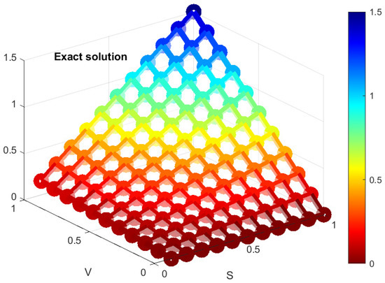
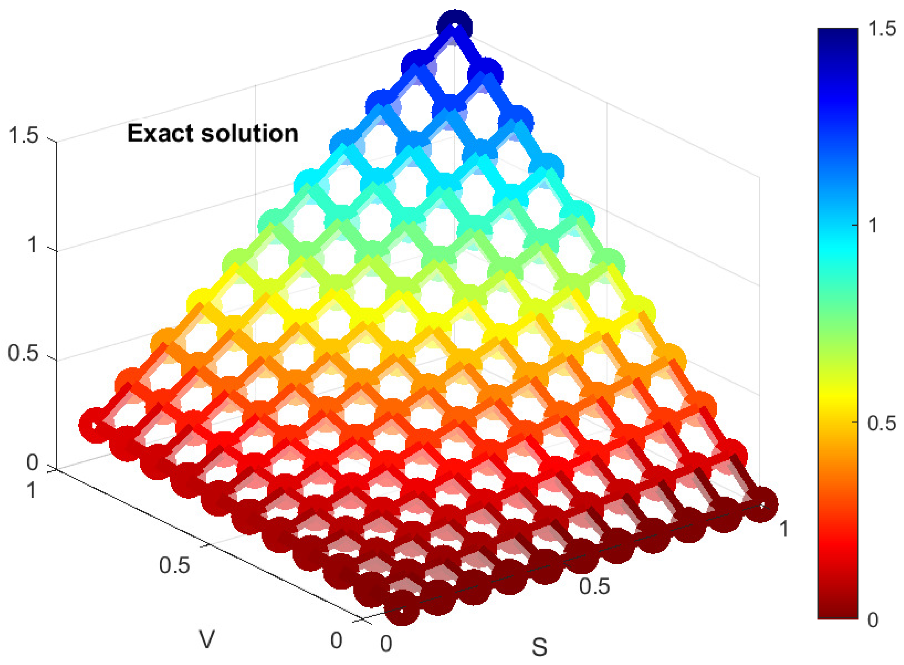
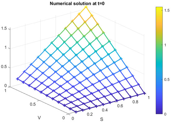
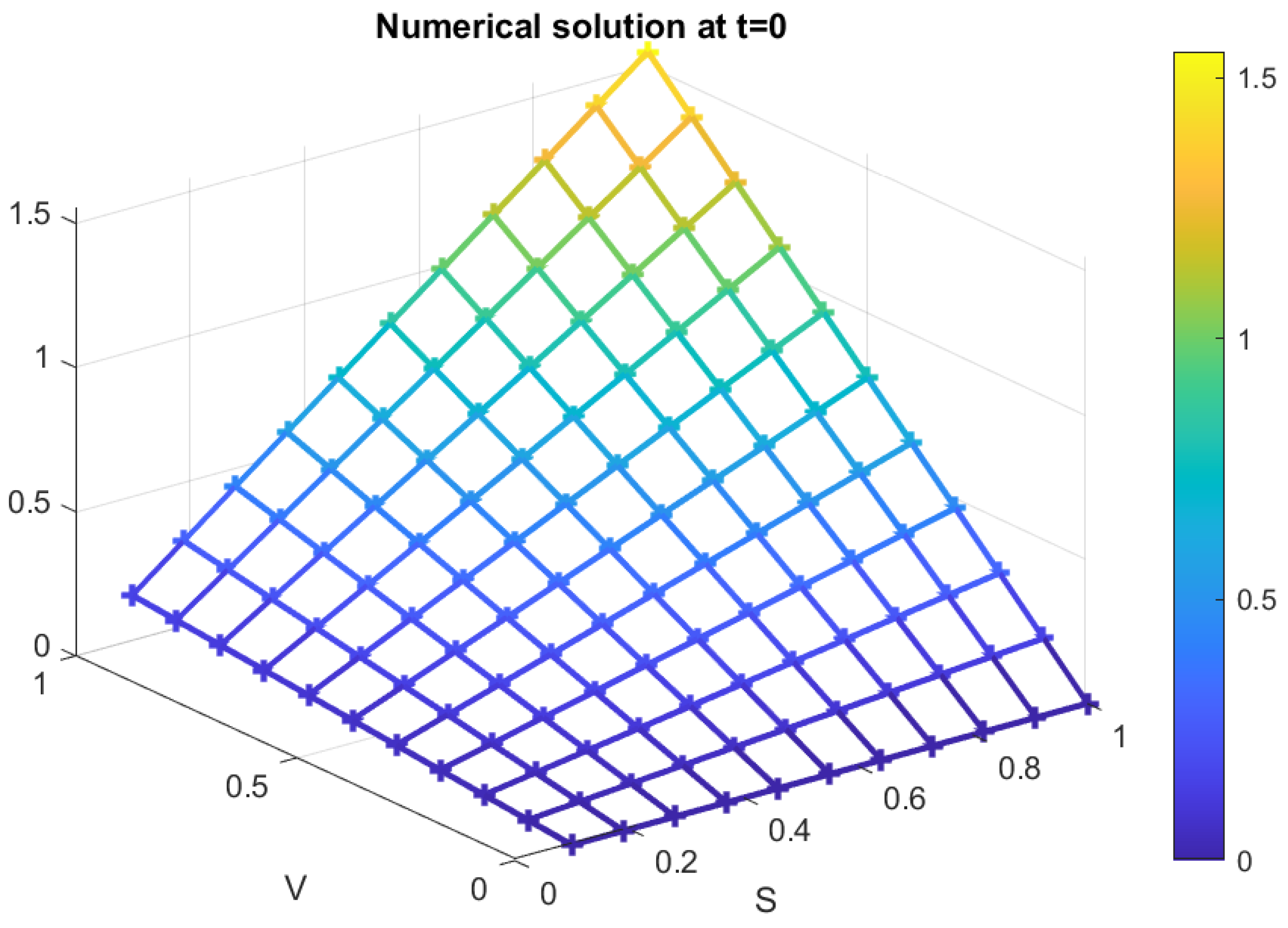
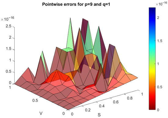
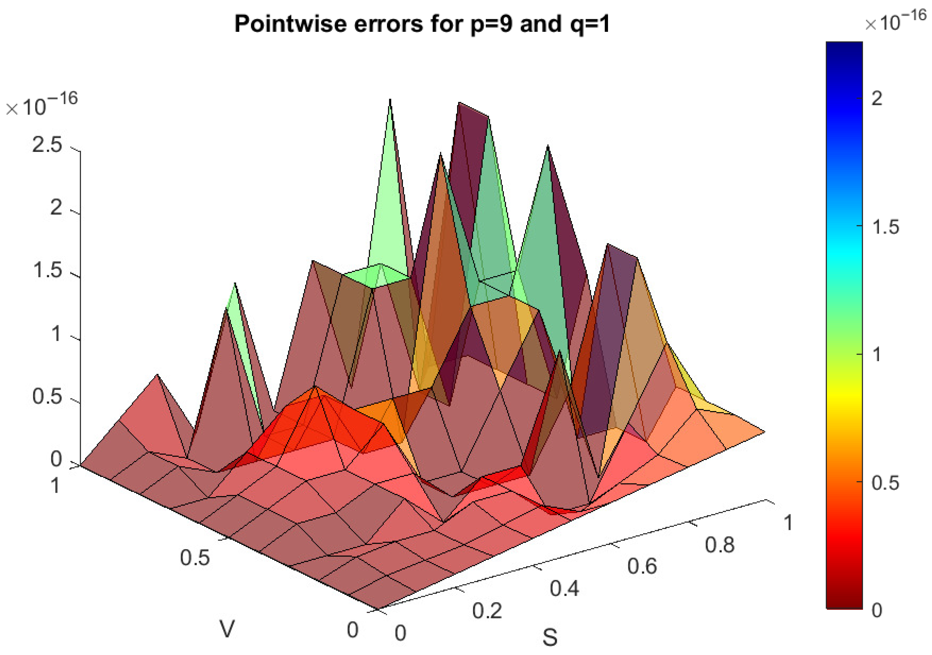
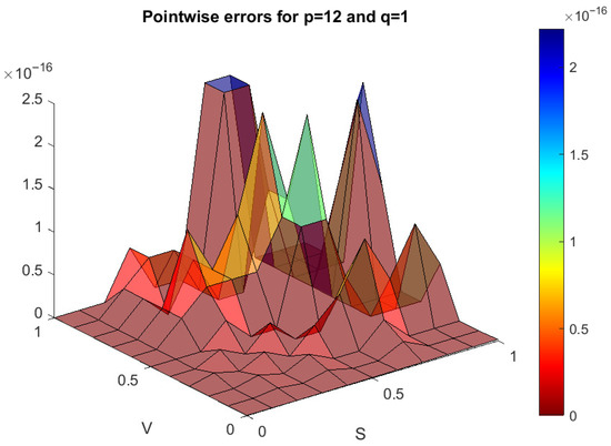
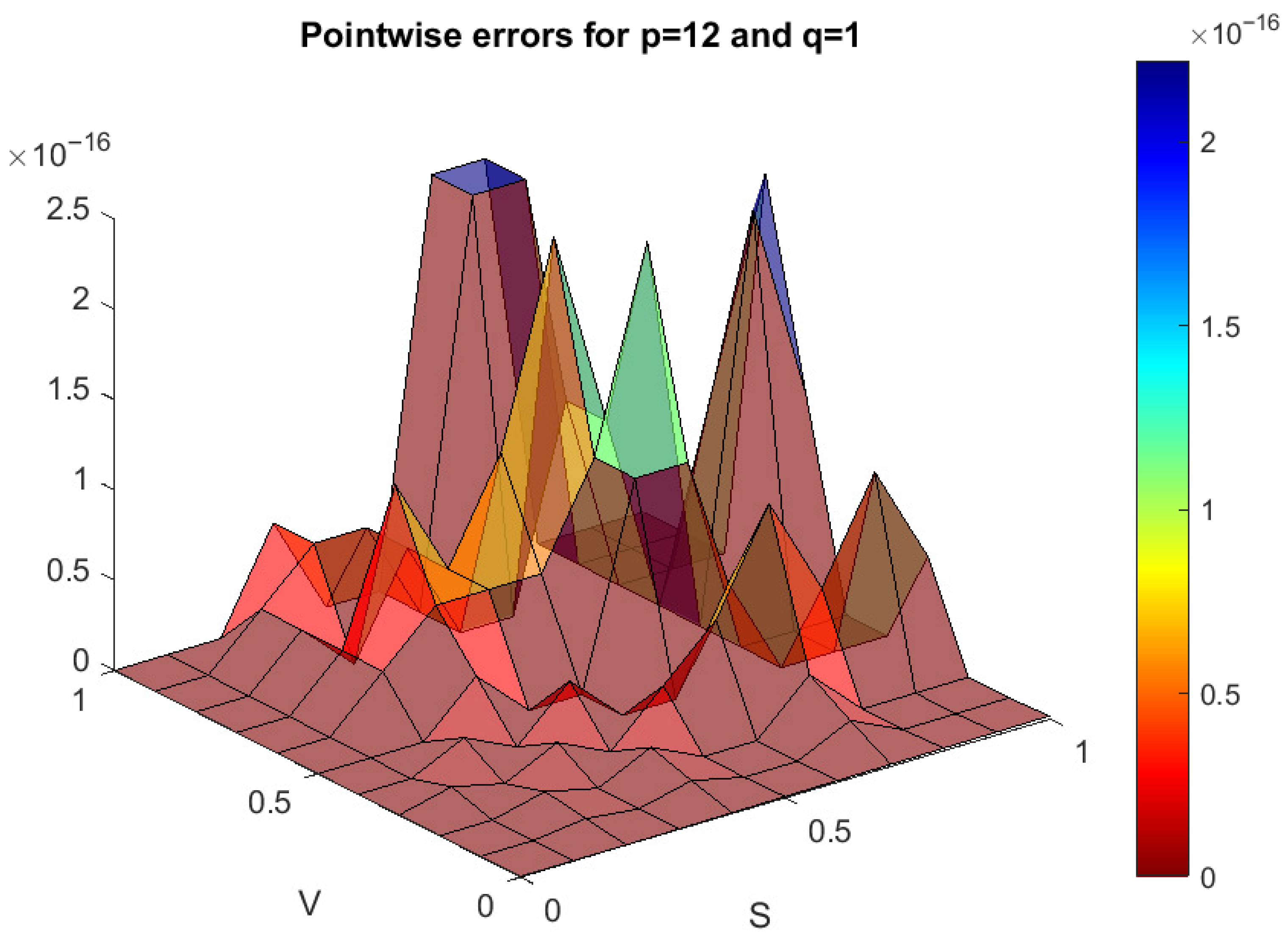
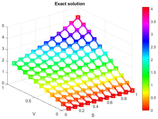
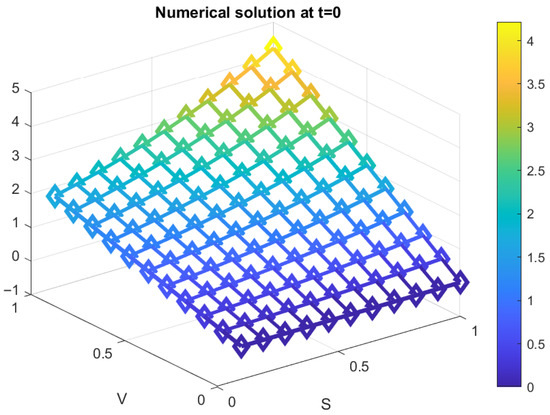
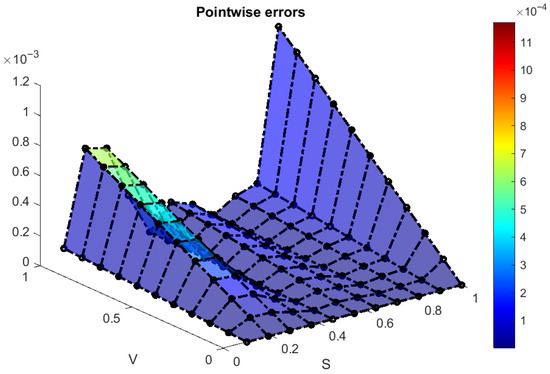
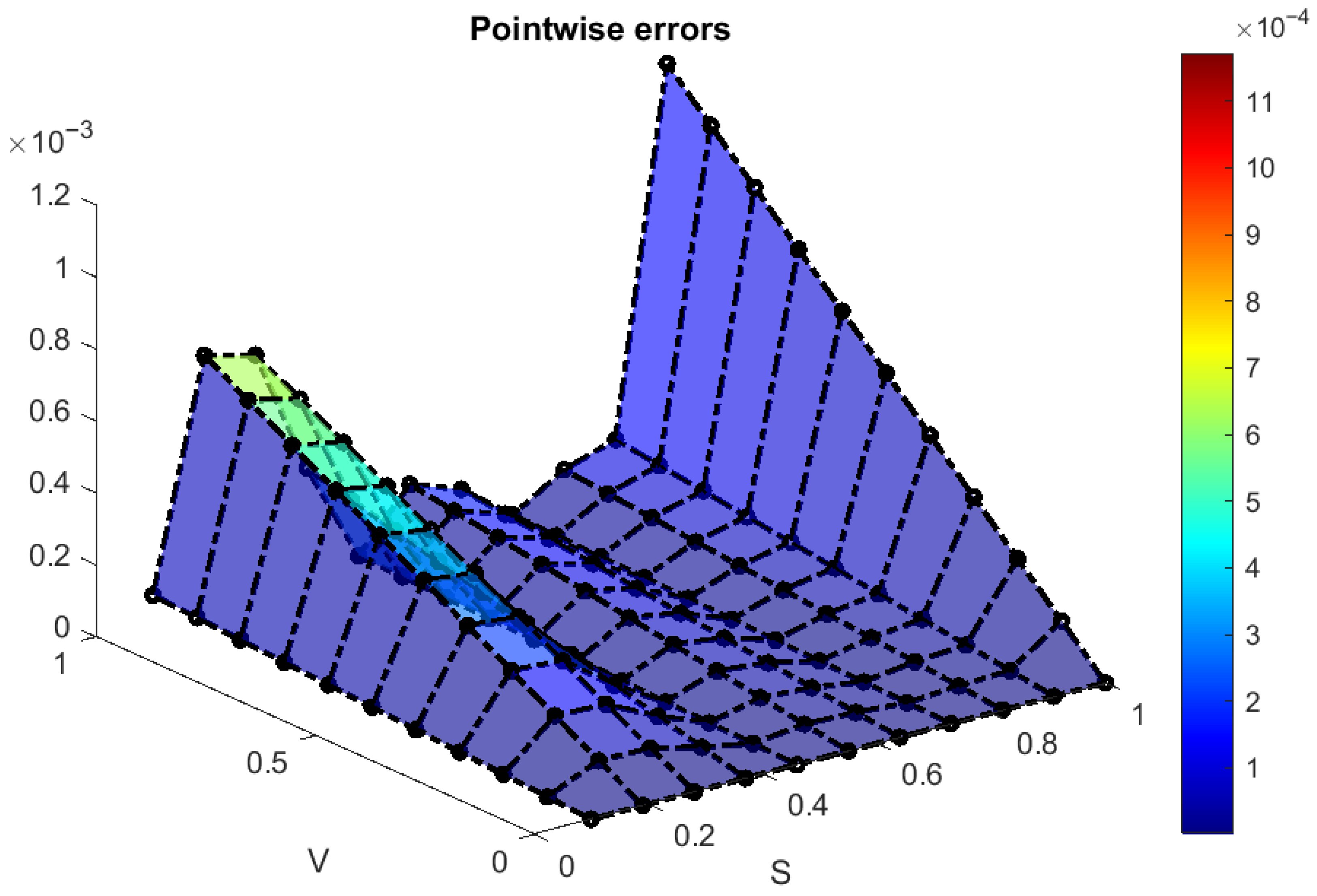
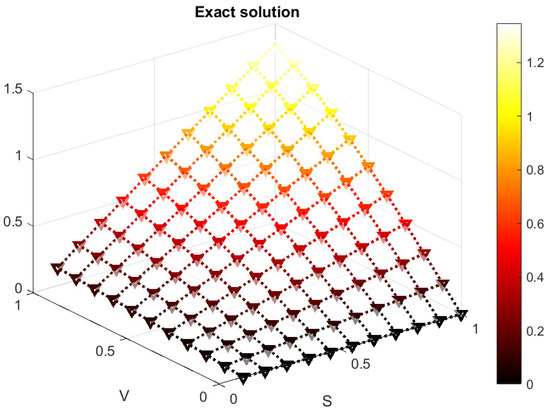
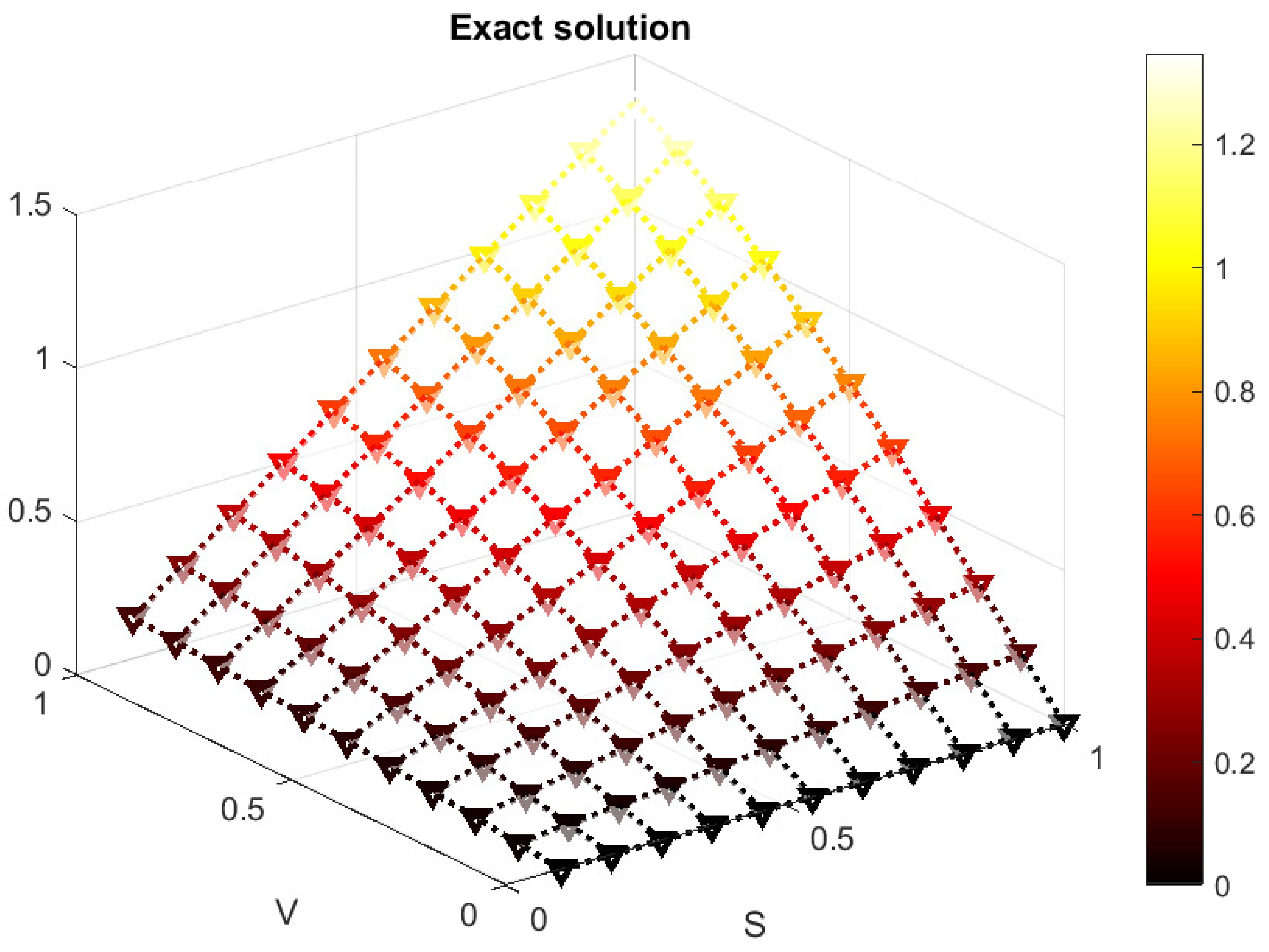
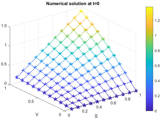
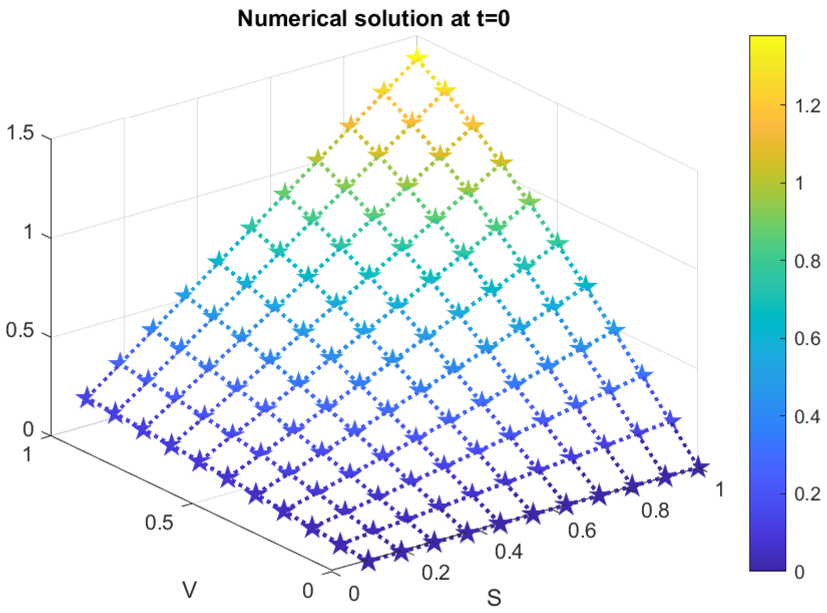
In this test problem, we apply the collocation method to approximate the solution of the problem. By choosing $(M,N,M^{\prime },N^{\prime })=(2,1,1,1)$ and computing the operational matrices, we obtain a system of algebraic equations. The absolute error of the method at sample points $(0,S_i,V_i,0.5)$ for different values of parameters p and q is gathered in Table 1. The parameters p and q in basis polynomials give us the freedom to change their values to obtain more accurate results. We can see that by increasing the value of parameter p, we obtain more accurate results. The graphical representations are illustrated in Figure 1, Figure 2, Figure 3, Figure 4, Figure 5 and Figure 6. It is clear that the numerical solution converges to the analytical solution.

Table 1. Absolute errors at points $(0,S_i,V_i,0.5)$ with $n^{\ast }=3$, $M=2$, $N=M^{\prime }=N^{\prime }=1$ for Example 1.

$(0,{\mathit{S}}_{\mathit{i}},{\mathit{V}}_{\mathit{i}},0.5)$	$\mathit{p}=2,\mathit{q}=1$	$\mathit{p}=4,\mathit{q}=1$	$\mathit{p}=9,\mathit{q}=1$	$\mathit{p}=12,\mathit{q}=1$
$(0,0,0,0.5)$	$1.1305\times {10}^{-16}$	$2.4125\times {10}^{-17}$	$3.1899\times {10}^{-26}$	$5.5030\times {10}^{-26}$
$(0,0.2,0.2,0.5)$	$1.4106\times {10}^{-11}$	$8.4540\times {10}^{-12}$	$1.3878\times {10}^{-17}$	$6.9389\times {10}^{-18}$
$(0,0.4,0.4,0.5)$	$3.5237\times {10}^{-10}$	$6.2182\times {10}^{-11}$	$2.7755\times {10}^{-17}$	$2.7755\times {10}^{-17}$
$(0,0.6,0.6,0.5)$	$1.0148\times {10}^{-9}$	$1.6118\times {10}^{-10}$	$5.5511\times {10}^{-17}$	$1.1102\times {10}^{-16}$
$(0,0.8,0.8,0.5)$	$2.0013\times {10}^{-9}$	$3.0546\times {10}^{-10}$	$0.0$	$0.0$
$(0,1,1,0.5)$	$3.3121\times {10}^{-9}$	$4.9501\times {10}^{-10}$	$0.0$	$0.0$
$CPU$	$1.0683s$	$0.8559s$	$0.6006s$	$0.5103s$

Figure 1. Analytical solution with $(M,N,M^{\prime },N^{\prime })=(2,1,1,1)$, $p=12$, $q=1$ at $t=0$ and $K=0.5$ for Example 1.

Figure 2. Approximate solution with $(M,N,M^{\prime },N^{\prime })=(2,1,1,1)$, $p=12$, $q=1$ at $t=0$ and $K=0.5$ for Example 1.

Figure 3. Error function with $(M,N,M^{\prime },N^{\prime })=(2,1,1,1)$, $p=2$, $q=1$ at $t=0$ and $K=0.5$ for Example 1.

Figure 4. Error function with $(M,N,M^{\prime },N^{\prime })=(2,1,1,1)$, $p=6$, $q=1$ at $t=0$ and $K=0.5$ for Example 1.

Figure 5. Error function with $(M,N,M^{\prime },N^{\prime })=(2,1,1,1)$, $p=9$, $q=1$ at $t=0$ and $K=0.5$ for Example 1.

Figure 6. Error function with $(M,N,M^{\prime },N^{\prime })=(2,1,1,1)$, $p=12$, $q=1$ at $t=0$ and $K=0.5$ for Example 1.

Example 2.

In this problem, the exact solution is $\mathcal{C}(t,S,V,K)=(t+1)e^{S}V(K+1)$ and

$$\begin{array}{cc}\hfill & {\displaystyle \frac{\partial \mathcal{C}(t,S,V,K)}{\partial t}}+rS{\displaystyle \frac{\partial \mathcal{C}(t,S,V,K)}{\partial S}}+rV{\displaystyle \frac{\partial \mathcal{C}(t,S,V,K)}{\partial V}}+{\displaystyle \frac{\partial \mathcal{C}(t,S,V,K)}{\partial K}}{\displaystyle \frac{dK\left(t\right)}{dt}}\hfill \\ & +(1+2H{t}^{2H-1})\left({\displaystyle \frac{1}{2}}V{S}^2{\displaystyle \frac{{\partial }^2\mathcal{C}(t,S,V,K)}{{\partial S}^2}}+{\displaystyle \frac{1}{2}}{\sigma }^{2}V{\displaystyle \frac{{\partial }^2\mathcal{C}(t,S,V,K)}{{\partial V}^2}}+\sigma VS{\displaystyle \frac{{\partial }^2\mathcal{C}(t,S,V,K)}{\partial V\partial S}}\right)\hfill \\ & -r\mathcal{C}(t,S,V,K)=\mathfrak{F}(t,S,V,K),\hfill \end{array}$$

with terminal and boundary conditions

$$\begin{array}{cc}\hfill & \mathcal{C}(1,S,V,K)=2e^{S}V(K+1),S\in [0.1,1],V\in [0,1],K\in [0.1,1],\hfill \\ & \mathcal{C}(t,0.1,V,K)=(t+1)e^{0.1}V(K+1),t\in [0,T],V\in [0,1],K\in [0.1,1],\hfill \\ & \mathcal{C}(t,1,V,K)=(t+1)eV(K+1),t\in [0,1],V\in [0,1],K\in [0.1,1],\hfill \\ & \mathcal{C}(t,S,0,K)=0,t\in [0,1],S\in [0.1,1],K\in [0.1,1],\hfill \\ & \mathcal{C}(t,S,1,K)=(t+1)e^S(K+1),t\in [0,1],S\in [0.1,1],K\in [0.1,1],\hfill \end{array}$$

where

$$\begin{array}{cc}\hfill \mathfrak{F}(t,S,V,K)& =e^{S}V(K+1)+rS(t+1)e^{S}V(K+1)+rV(t+1)e^S(K+1)\hfill \\ & +rKS(t+1)e^{S}V{\displaystyle \frac{n^{\ast }ln\left(S\right)-ln\left(K\right)}{t}}+(1+2H{t}^{2H-1}){\displaystyle \frac{1}{2}}V{S}^2(t+1)e^{S}V(k+1)\hfill \\ & +(1+2H{t}^{2H-1})\sigma (t+1)VS{e}^S(K+1)-r(t+1)e^{S}V(K+1).\hfill \end{array}$$

The parameters are as follows

$$r=0.1,\sigma =0.1,H=0.8.$$

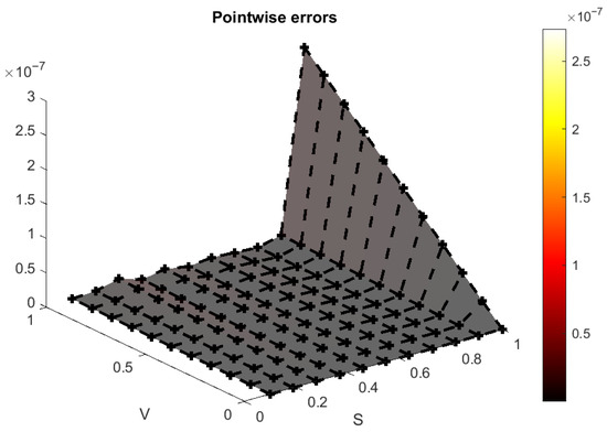
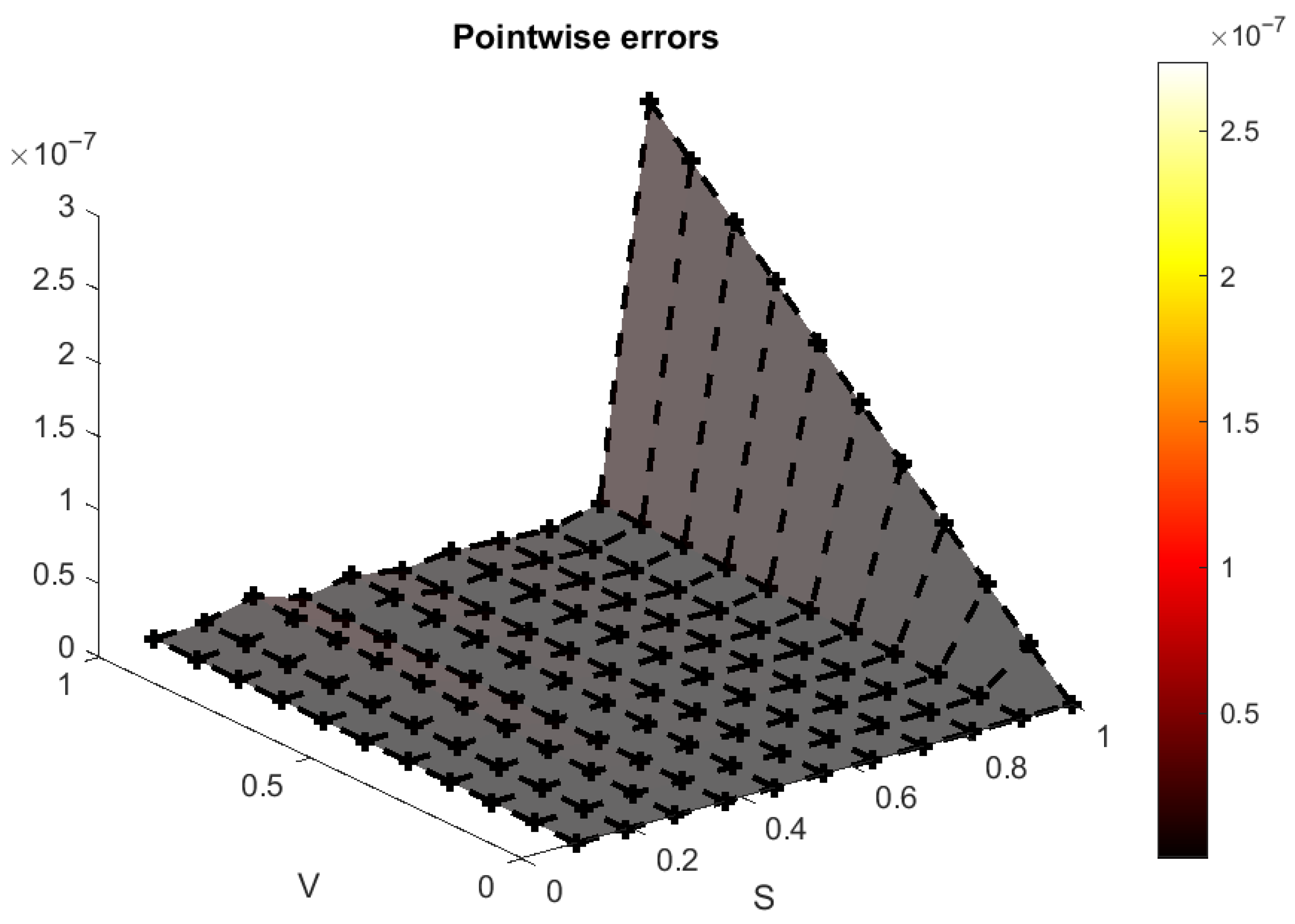
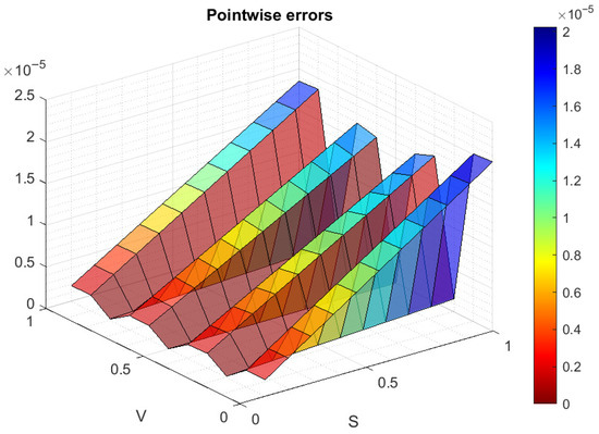
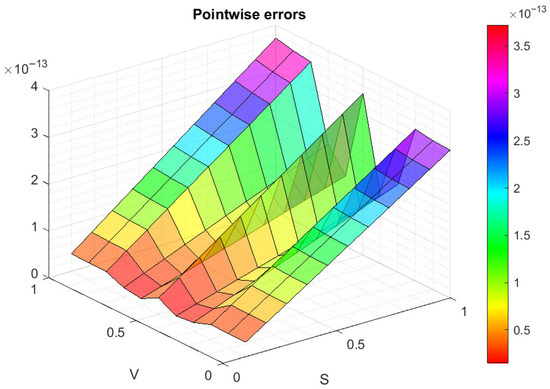
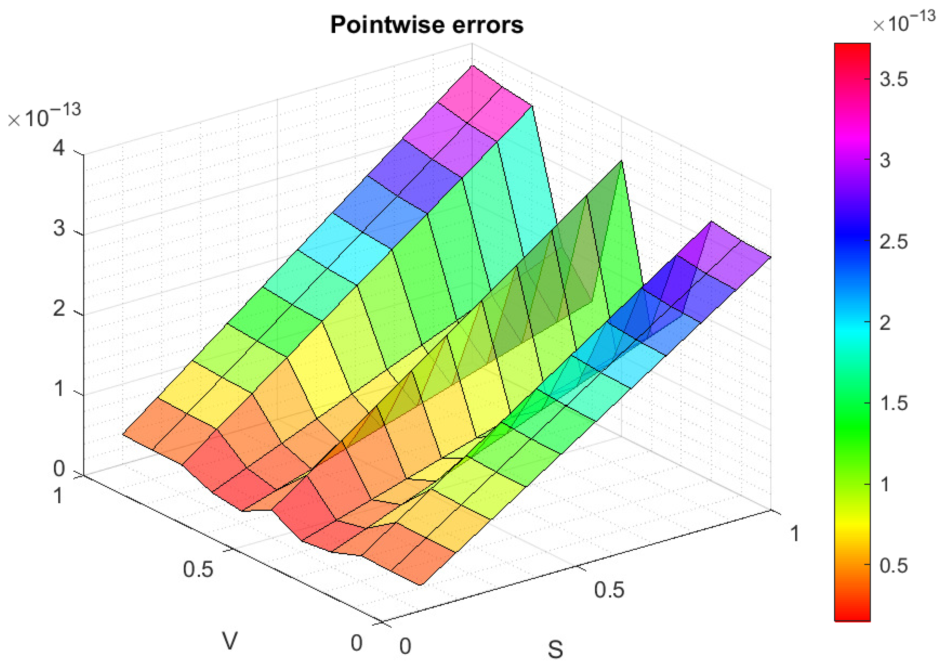
The absolute errors at points $(0,S_i,V_i,0.5)$ with $n^{\ast }=3$, $p=1000$, $q=1$, $N=M^{\prime }=N^{\prime }=1$ and different values of M are provided in Table 2. As can be seen from the table, the absolute amount of error is reduced by increasing the parameter value of the M. The CPU is also collected in Table 2, which indicates the appropriate speed of the method. Figure 7 and Figure 8 show that the numerical solution is very close to the exact one. Also, error functions are depicted in Figure 9, Figure 10, Figure 11 and Figure 12. These shapes indicate that the remainder term converges to zero and this corresponds to the results of the theory.

Table 2. Absolute errors at points $(0,S_i,V_i,0.5)$ with $n^{\ast }=3$, $p=1000$, $q=1$ and $N=M^{\prime }=N^{\prime }=1$ for Example 2.

$(0,{\mathit{S}}_{\mathit{i}},{\mathit{V}}_{\mathit{i}},0.5)$	$\mathit{M}=4$	$\mathit{M}=7$	$\mathit{M}=10$	$\mathit{M}=12$
$(0,0.1,0.1,0.5)$	$8.9754\times {10}^{-16}$	$3.2217\times {10}^{-16}$	$7.4855\times {10}^{-16}$	$2.7617\times {10}^{-16}$
$(0,0.2,0.2,0.5)$	$1.3298\times {10}^{-4}$	$2.3698\times {10}^{-9}$	$2.1150\times {10}^{-14}$	$9.4369\times {10}^{-16}$
$(0,0.4,0.4,0.5)$	$1.2382\times {10}^{-5}$	$2.8417\times {10}^{-9}$	$7.9936\times {10}^{-15}$	$2.2204\times {10}^{-16}$
$(0,0.6,0.6,0.5)$	$8.4010\times {10}^{-5}$	$2.8305\times {10}^{-9}$	$3.3529\times {10}^{-14}$	$1.9984\times {10}^{-15}$
$(0,0.8,0.8,0.5)$	$9.4687\times {10}^{-5}$	$3.9214\times {10}^{-10}$	$3.1086\times {10}^{-14}$	$1.7763\times {10}^{-15}$
$(0,1,1,0.5)$	$1.1716\times {10}^{-3}$	$2.7357\times {10}^{-7}$	$2.2015\times {10}^{-11}$	$4.1922\times {10}^{-13}$
$CPU$	$0.9341s$	$1.2280s$	$1.0651s$	$1.0491s$

Figure 7. Analytical solution with $(M,N,M^{\prime },N^{\prime })=(4,1,1,1)$, $p=1000$, $q=1$ at $t=0$ and $K=0.5$ for Example 2.

Figure 8. Approximate solution with $(M,N,M^{\prime },N^{\prime })=(4,1,1,1)$, $p=1000$, $q=1$ at $t=0$ and $K=0.5$ for Example 2.

Figure 9. Error function with $(M,N,M^{\prime },N^{\prime })=(4,1,1,1)$, $p=1000$, $q=1$ at $t=0$ and $K=0.5$ for Example 2.

Figure 10. Error function with $(M,N,M^{\prime },N^{\prime })=(7,1,1,1)$, $p=1000$, $q=1$ at $t=0$ and $K=0.5$ for Example 2.

Figure 11. Error function with $(M,N,M^{\prime },N^{\prime })=(10,1,1,1)$, $p=1000$, $q=1$ at $t=0$ and $K=0.5$ for Example 2.

Figure 12. Error function with $(M,N,M^{\prime },N^{\prime })=(12,1,1,1)$, $p=1000$, $q=1$ at $t=0$ and $K=0.5$ for Example 2.

Example 3.

In this problem, the exact solution is $\mathcal{C}(t,S,V,K)=(t^2+1)Ssin\left(V\right)(K+1)$ and

$$\begin{array}{cc}\hfill & {\displaystyle \frac{\partial \mathcal{C}(t,S,V,K)}{\partial t}}+rS{\displaystyle \frac{\partial \mathcal{C}(t,S,V,K)}{\partial S}}+rV{\displaystyle \frac{\partial \mathcal{C}(t,S,V,K)}{\partial V}}+{\displaystyle \frac{\partial \mathcal{C}(t,S,V,K)}{\partial K}}{\displaystyle \frac{dK\left(t\right)}{dt}}\hfill \\ & +(1+2H{t}^{2H-1})\left({\displaystyle \frac{1}{2}}V{S}^2{\displaystyle \frac{{\partial }^2\mathcal{C}(t,S,V,K)}{{\partial S}^2}}+{\displaystyle \frac{1}{2}}{\sigma }^{2}V{\displaystyle \frac{{\partial }^2\mathcal{C}(t,S,V,K)}{{\partial V}^2}}+\sigma VS{\displaystyle \frac{{\partial }^2\mathcal{C}(t,S,V,K)}{\partial V\partial S}}\right)\hfill \\ & -r\mathcal{C}(t,S,V,K)=\mathfrak{F}(t,S,V,K),\hfill \end{array}$$

with terminal and boundary conditions

$$\begin{array}{cc}\hfill & \mathcal{C}(1,S,V,K)=2Ssin\left(V\right)(K+1),S\in [0.1,1],V\in [0,1],K\in [0.1,1],\hfill \\ & \mathcal{C}(t,0,V,K)=0.1(t^2+1)sin\left(V\right)(K+1),t\in [0,T],V\in [0,1],K\in [0.1,1],\hfill \\ & \mathcal{C}(t,1,V,K)=(t^2+1)sin\left(V\right)(K+1),t\in [0,1],V\in [0,1],K\in [0.1,1],\hfill \\ & \mathcal{C}(t,S,0,K)=0,t\in [0,1],S\in [0.1,1],K\in [0.1,1],\hfill \\ & \mathcal{C}(t,S,1,K)=(t^2+1)Ssin\left(1\right)(K+1),t\in [0,1],S\in [0.1,1],K\in [0.1,1],\hfill \end{array}$$

where

$$\begin{array}{cc}\hfill \mathfrak{F}(t,S,V,K)& =2tSsin\left(V\right)(K+1)+rS(t^2+1)sin\left(V\right)(K+1)+rV(t^2+1)Scos\left(V\right)(K+1)\hfill \\ & +rKS(t^2+1)Ssin\left(V\right){\displaystyle \frac{n^{\ast }ln\left(S\right)-ln\left(K\right)}{t}}-(1+2H{t}^{2H-1}){\displaystyle \frac{1}{2}}{\sigma }^{2}V(t^2+1)Ssin\left(V\right)(K+1)\hfill \\ & +(1+2H{t}^{2H-1})\sigma (t^2+1)VScos\left(V\right)(K+1)-r(t^2+1)Ssin\left(V\right)(K+1).\hfill \end{array}$$

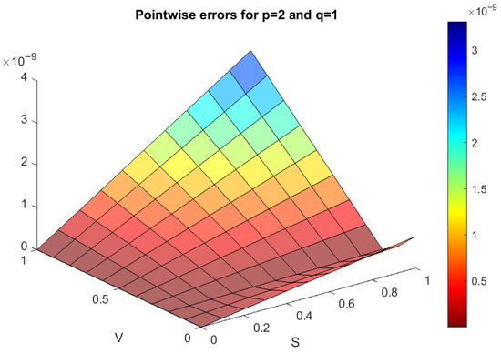
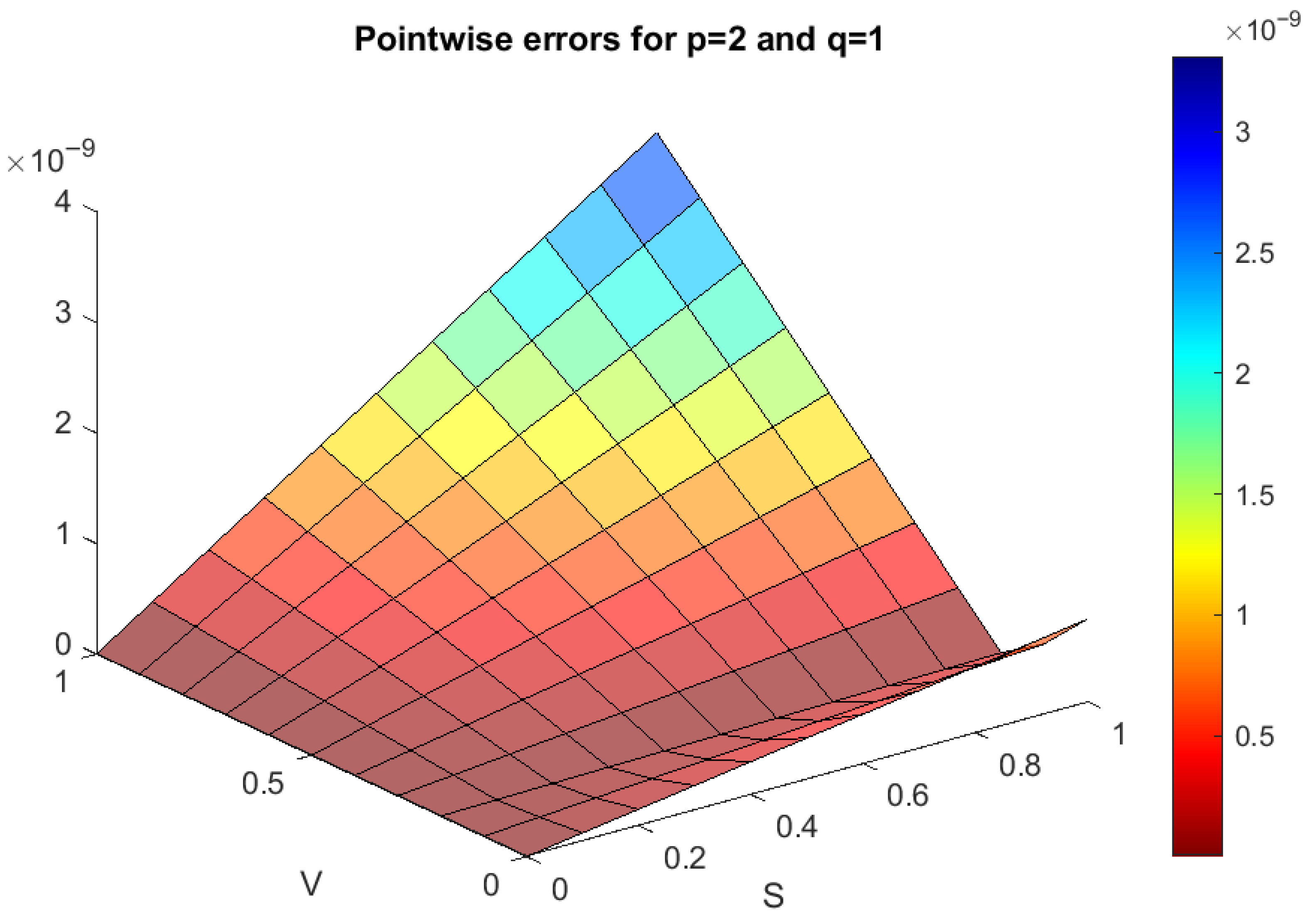
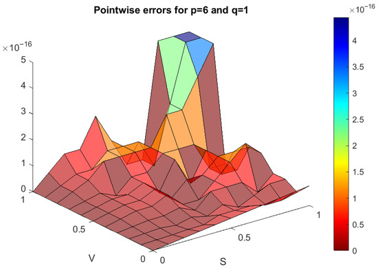
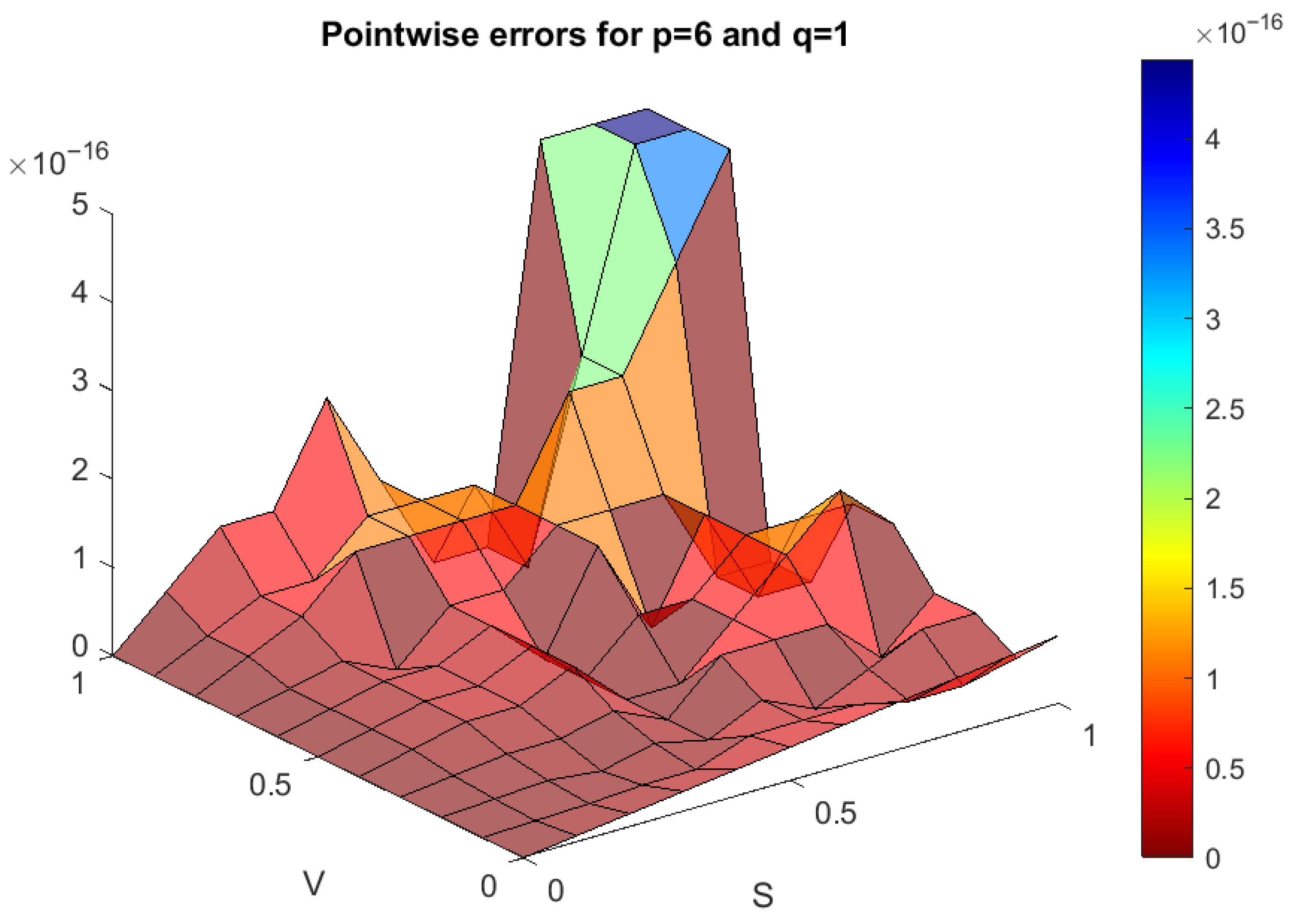
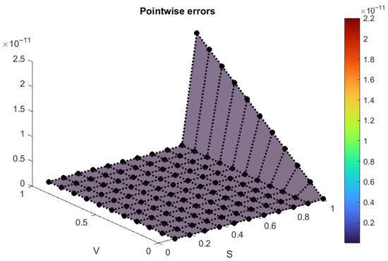
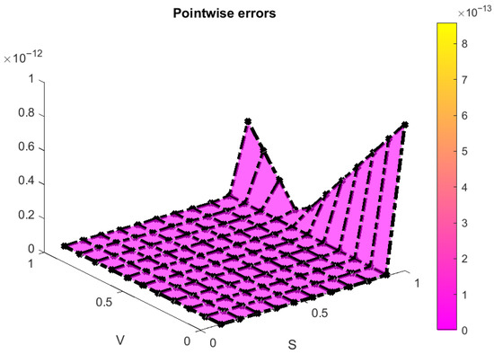
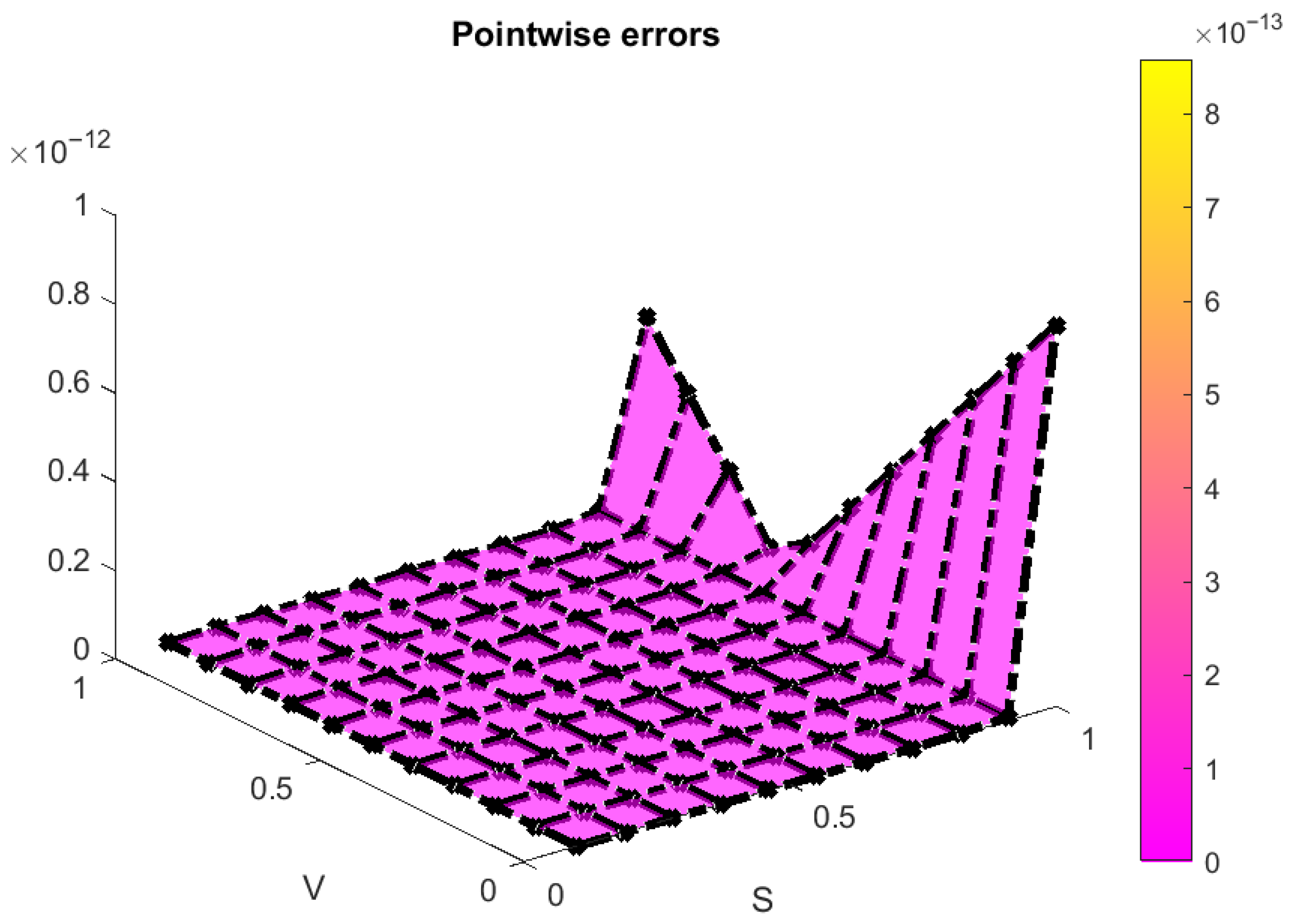
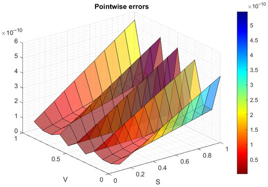
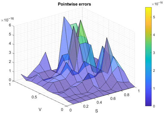
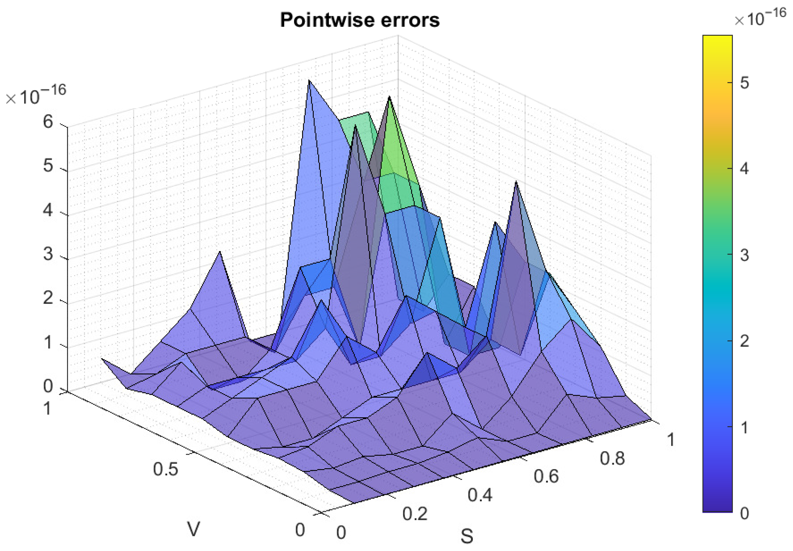
Parameters r, σ, and H are the same as before. The numerical results are reported in Table 3. In $t=0$ and $K=0.6$ for sample points $(0,S_i,K_i,0.6)$, the absolute errors show that our numerical approach works very well. The exact and numerical solutions are depicted in Figure 13 and Figure 14. Also, the surfaces of pointwise errors are illustrated in Figure 15, Figure 16, Figure 17 and Figure 18. We can see that the error function tends to zero. All tables and figures show the applicability and efficiency of the presented numerical scheme.

Table 3. Absolute errors at points $(0,S_i,V_i,0.6)$ with $n^{\ast }=3$, $p=1000$, $q=1$ and $N=N^{\prime }=1$ for Example 3.

$(0,{\mathit{S}}_{\mathit{i}},{\mathit{V}}_{\mathit{i}},0.6)$	$\mathit{M}=2,{\mathit{M}}^{\prime }=4$	$\mathit{M}=2,{\mathit{M}}^{\prime }=7$	$\mathit{M}=2,{\mathit{M}}^{\prime }=9$	$\mathit{M}=2,{\mathit{M}}^{\prime }=13$
$(0,0.1,0.1,0.6)$	$2.2047\times {10}^{-6}$	$4.8352\times {10}^{-11}$	$3.4335\times {10}^{-14}$	$9.7597\times {10}^{-18}$
$(0,0.2,0.2,0.6)$	$4.6173\times {10}^{-7}$	$5.9827\times {10}^{-11}$	$9.8532\times {10}^{-14}$	$2.7755\times {10}^{-17}$
$(0,0.4,0.4,0.6)$	$8.3186\times {10}^{-6}$	$9.7434\times {10}^{-12}$	$7.2664\times {10}^{-14}$	$1.1102\times {10}^{-16}$
$(0,0.6,0.6,0.6)$	$1.1364\times {10}^{-5}$	$1.4120\times {10}^{-11}$	$1.0514\times {10}^{-13}$	$2.2204\times {10}^{-16}$
$(0,0.8,0.8,0.6)$	$1.2801\times {10}^{-6}$	$1.9801\times {10}^{-10}$	$3.1886\times {10}^{-13}$	$1.1102\times {10}^{-15}$
$(0,1,1,0.6)$	$2.0120\times {10}^{-5}$	$5.9317\times {10}^{-10}$	$4.0612\times {10}^{-13}$	$8.8818\times {10}^{-16}$
$CPU$	$0.9035s$	$1.3634s$	$1.3037s$	$1.8678s$

Figure 13. Analytical solution with $(M,N,M^{\prime },N^{\prime })=(2,1,13,1)$, $p=1000$, $q=1$ at $t=0$ and $K=0.6$ for Example 3.

Figure 14. Approximate solution with $(M,N,M^{\prime },N^{\prime })=(2,1,13,1)$, $p=1000$, $q=1$ at $t=0$ and $K=0.6$ for Example 3.

Figure 15. Error function with $(M,N,M^{\prime },N^{\prime })=(2,1,4,1)$, $p=1000$, $q=1$ at $t=0$ and $K=0.6$ for Example 3.

Figure 16. Error function with $(M,N,M^{\prime },N^{\prime })=(2,1,7,1)$, $p=1000$, $q=1$ at $t=0$ and $K=0.6$ for Example 3.

Figure 17. Error function with $(M,N,M^{\prime },N^{\prime })=(2,1,9,1)$, $p=1000$, $q=1$ at $t=0$ and $K=0.6$ for Example 3.

Figure 18. Error function with $(M,N,M^{\prime },N^{\prime })=(2,1,13,1)$, $p=1000$, $q=1$ at $t=0$ and $K=0.6$ for Example 3.

Table 4 presents a comparison between the proposed collocation method and the Monte Carlo simulation approach of [4] for pricing geometric Asian options under the mixed fractional Heston model. The comparison is performed for different strike prices $K=0.6,0.7,0.8,0.9$ and varying numbers of antithetic variables $O=2,4,6,8$ in the Monte Carlo simulation. The results demonstrate that the present method yields consistent option prices ($0.3821$, $0.2684$, $0.1730$, and $0.0844$ for $K=0.6,0.7,0.8,0.9$, respectively) that are independent of the number of antithetic variables, whereas the Monte Carlo estimates exhibit slight variations as O increases. Notably, the values obtained by the proposed collocation method converge to values that are slightly lower than the Monte Carlo estimates for all strike prices, with the difference diminishing as the number of antithetic variables increases. This comparison validates the accuracy and robustness of the proposed spectral collocation approach, which achieves deterministic results without the statistical variability inherent in Monte Carlo methods.

Table 4. Comparison of the present method and the Monte Carlo simulation ([4]) for different numbers of antithetic variables $\left(O\right)$ and strike prices $\left(K\right)$.

	O = 2	O = 4	O = 6	O = 8
Monte-Carlo Method (K = 0.6)	0.3915	0.3869	0.3843	0.3832
Present Method	0.3821	0.3821	0.3821	0.3821
Monte-Carlo Method (K = 0.7)	0.2709	0.2693	0.2689	0.2687
Present Method	0.2684	0.2684	0.2684	0.2684
Monte-Carlo Method (K = 0.8)	0.0.1762	0.1750	0.1741	0.1737
Present Method	0.1730	0.1730	0.1730	0.1730
Monte-Carlo Method (K = 0.9)	0.0907	0.0881	0.0859	0.08503
Present Method	0.0844	0.0844	0.0844	0.0844

6. Conclusions

This paper has successfully developed and validated a novel computational framework for pricing geometric Asian options within the fractional Heston model. By leveraging a collocation method based on diagonal polynomials, we constructed sparse operational matrices that significantly enhance computational efficiency. Our approach transformed the governing PDE into a tractable system of nonlinear algebraic equations, for which we also provided a rigorous convergence analysis. The comprehensive numerical experiments demonstrated the method’s notable applicability, robustness, and performance. The strong synergy between the theoretical underpinnings and the compelling numerical results confirms that this method is not only effective but also holds considerable promise for practical application in financial engineering. Future work could focus on extending this framework to other complex path-dependent derivatives and multi-asset options.

References

- Abdi, N.; Aminikhah, H.; Sheikhani, A.R. High-order compact finite difference schemes for the time-fractional Black-Scholes model governing European options. Chaos Solitons Fractals 2022, 162, 112423. [Google Scholar] [CrossRef] [Scilit]
- Tian, Z.; Zhai, S.; Weng, Z. Compact finite difference schemes of the time fractional Black-Scholes model. J. Appl. Anal. Comput. 2020, 10, 904–919. [Google Scholar] [CrossRef] [Scilit] [PubMed]
- Mehrdoust, F. A new hybrid Monte Carlo simulation for Asian options pricing. J. Stat. Comput. Simul. 2015, 85, 507–516. [Google Scholar] [CrossRef] [Scilit]
- Najafi, A.; Mehrdoust, F. Conditional expectation strategy under the long memory Heston stochastic volatility model. Commun. Stat. Simul. Comput. 2024, 53, 5453–5473. [Google Scholar] [CrossRef] [Scilit]
- Golbabai, A.; Nikan, O.; Nikazad, T. Numerical analysis of time fractional Black–Scholes European option pricing model arising in financial market. Comput. Appl. Math. 2019, 38, 173. [Google Scholar] [CrossRef] [Scilit]
- Sawangtong, P.; Taghipour, M.; Najafi, A. An efficient computational method for solving the fractional form of the European option price PDE with transaction cost under the fractional Heston model. Eng. Anal. Bound. Elem. 2024, 169, 105972. [Google Scholar] [CrossRef] [Scilit]
- Taghipour, M.; Aminikhah, H. A spectral collocation method based on fractional Pell functions for solving time–fractional Black–Scholes option pricing model. Chaos Solitons Fractals 2022, 163, 112571. [Google Scholar] [CrossRef] [Scilit]
- Mesgarani, H.; Beiranvand, A.; Esmaeelzade Aghdam, Y. The impact of the Chebyshev collocation method on solutions of the time-fractional Black–Scholes. Math. Sci. 2021, 15, 137–143. [Google Scholar] [CrossRef] [Scilit]
- Badawi, H.; Arqub, O.A.; Shawagfeh, N. Theoretical study and numerical analysis using step spectral collocation method for stochastic M-fractional differential models of simplified Brownian motion within constant delays process. J. Appl. Math. Comput. 2025, 71, 6773–6805. [Google Scholar] [CrossRef] [Scilit]
- Sawangtong, P.; Najafi, A. Collocation method with Morgan-Voyce polynomials to solve the time fractional long memory Black-Scholes model with jump process. J. Appl. Math. Comput. 2025, 71, 8123–8161. [Google Scholar] [CrossRef] [Scilit]
- Mangal, S.; Gupta, V. Exponential B-spline collocation method with Richardson extrapolation for generalized Black-Scholes equation. J. Appl. Math. Comput. 2025, 71, 3965–3995. [Google Scholar] [CrossRef] [Scilit]
- Ma, P.; Taghipour, M.; Cattani, C. Option pricing in the illiquid markets under the mixed fractional Brownian motion model. Chaos Solitons Fractals 2024, 182, 114806. [Google Scholar] [CrossRef] [Scilit]
- Mehrdoust, F.; Najafi, A.R.; Fallah, S.; Samimi, O. Mixed fractional Heston model and the pricing of American options. J. Comput. Appl. Math. 2018, 330, 141–154. [Google Scholar] [CrossRef] [Scilit]
- Alazemi, F.; Douissi, S.; Es-Sebaiy, K. Berry–Esseen Bounds and ASCLTs for Drift Parameter Estimator of Mixed Fractional Ornstein–Uhlenbeck Process with Discrete Observations. Theory Probab. Its Appl. 2019, 64, 401–420. [Google Scholar] [CrossRef] [Scilit]
- Shi, Q.; Yang, X. Pricing Asian options in a stochastic volatility model with jumps. Appl. Math. Comput. 2014, 228, 411–422. [Google Scholar] [CrossRef] [Scilit]
- Wang, W.; Cai, G.; Tao, X. Pricing geometric asian power options in the sub-fractional brownian motion environment. Chaos Solitons Fractals 2021, 145, 110754. [Google Scholar] [CrossRef] [Scilit]
- Alsenafi, A.; Alazemi, F.; Najafi, A. Geometric Asian power option pricing with transaction cost under the geometric fractional Brownian motion with w sources of risk in fuzzy environment. J. Comput. Appl. Math. 2025, 453, 116165. [Google Scholar] [CrossRef] [Scilit]
- Abdelhakem, M.; Abdelhamied, D.; El-Kady, M.; Youssri, Y.H. Two modified shifted Chebyshev–Galerkin operational matrix methods for even-order partial boundary value problems. Bound. Value Probl. 2025, 2025, 34. [Google Scholar] [CrossRef] [Scilit]
- Abd-Elhameed, W.M.; Youssri, Y.H.; Atta, A.G. Adopted spectral tau approach for the time-fractional diffusion equation via seventh-kind Chebyshev polynomials. Bound. Value Probl. 2024, 2024, 102. [Google Scholar] [CrossRef] [Scilit]
- Horadam, A.F. Extensions of a paper on diagonal functions. Fibonacci Q. 1980, 18, 3–6. [Google Scholar] [CrossRef] [Scilit]
Disclaimer/Publisher’s Note: The statements, opinions and data contained in all publications are solely those of the individual author(s) and contributor(s) and not of MDPI and/or the editor(s). MDPI and/or the editor(s) disclaim responsibility for any injury to people or property resulting from any ideas, methods, instructions or products referred to in the content. |
© 2026 by the authors. Licensee MDPI, Basel, Switzerland. This article is an open access article distributed under the terms and conditions of the Creative Commons Attribution (CC BY) license.