A Novel Inertial-Type Iteration Algorithm: Convergence, Data Dependence, and Applications in Image Deblurring and Fractal Generation

Abstract

This study introduces a novel inertial-type iteration algorithm based on the Normal S iteration for the class of almost contraction mappings in Banach spaces. Traditional fixed point iterations often suffer from slow convergence and high computational cost; to address these limitations, the proposed framework incorporates an adaptive inertial-type parameter. We establish strong convergence of the algorithm and derive explicit a posteriori error estimates under weak contractive conditions. In addition, we demonstrate the asymptotic equivalence of the NS inertial-type trajectories with the classical Normal S iteration, provide a comprehensive weak $w^2$—stability analysis, and obtain sharp upper bounds for the data dependence problem. The practical performance of the algorithm is evaluated in two distinct computational domains: image deblurring via wavelet-based ${\mathrm{\ell }}_1$ regularization and the generation of complex fractal patterns, including Julia and Mandelbrot sets. Numerical results show that the proposed inertial-type iteration algorithm significantly outperforms existing methods—such as Picard, Mann, Ishikawa, and standard Normal S iterations—achieving faster convergence, higher PSNR values in image restoration, and more stable basins of attraction in fractal visualizations. These findings highlight the effectiveness and versatility of the NS inertial-type iteration algorithm approach for both theoretical analysis and real-world applications.

1. Introduction

Throughout this study, we denote the set of natural numbers as $\mathbb{N}$, and $\mathcal{S}$ we represents a nonempty, closed, and convex subset of a Banach space $\mathcal{B}$ equipped with the norm $∥·∥$. Let $\mathbb{T}:\mathcal{S}\to \mathcal{S}$ be a mapping; a point x satisfying the equation $\mathbb{T}x=x$ is called a fixed point of $\mathbb{T}$, and the set of all fixed points within $\mathcal{S}$ is denoted by $Fix\left(\mathbb{T}\right)$.

Fixed point theory plays a fundamental role in solving problems encountered across a broad spectrum—from mathematical analysis to differential equations, from optimization to game theory, and even including data science. By investigating the existence, uniqueness, and numerical approximation of points mapped onto themselves by a mapping, this theory provides a framework for modeling the dynamics of complex systems. The cornerstone of this theory is the Banach Fixed Point Theorem, introduced by Stefan Banach in his groundbreaking 1922 work [1]. This theorem guarantees that for a contraction mapping $\mathbb{T}:\mathcal{S}\to \mathcal{S}$ satisfying the inequality

$$∥\mathbb{T}x-\mathbb{T}y∥\le \lambda ∥x-y∥,$$

(1)

for all $x,y\in \mathcal{S}$ with a constant $\lambda \in \left[0,1\right)$, the set $Fix\left(\mathbb{T}\right)$ consists of exactly one point. The Picard iteration $x_{n+1}=\mathbb{T}{x}_n$, used to approximate this fixed point numerically, forms the basis for numerous numerical methods and algorithms.

However, the classical contraction condition entails two significant limitations: the necessity for the mapping to be continuous and the requirement that $\lambda \in \left[0,1\right)$. These constraints narrow the scope of the theory in practical applications, highlighting the need for generalized frameworks that encompass broader classes of mappings. One important generalization developed in response to this need is the class of weak contractions introduced by Osilike [2]. This class includes mappings that satisfy the condition

$$∥\mathbb{T}x-\mathbb{T}y∥\le \lambda ∥x-y∥+L∥x-\mathbb{T}x∥.$$

(2)

for all $x,y\in \mathcal{S}$, where $\lambda \in \left[0,1\right)$ and $L\ge 0$ are constants. Nevertheless, as demonstrated in the example below, condition (2) does not always guarantee that $Fix\left(\mathbb{T}\right)\ne Ø$.

Example 1.

Let $\mathcal{B}=\mathbb{R}$ and $\mathcal{S}=\left[0,2\right]$ be equipped with the standard absolute value norm. Define the mapping $\mathbb{T}:\mathcal{S}\to \mathcal{S}$ as follows:

$$\mathbb{T}x=\left\{\begin{array}{cc}x+1,& x\in \left[0,1\right],\\ x-1,& x\in \left(1,2\right].\end{array}\right.$$

We now show that this mapping satisfies condition (2).

Case 1: If $x,y\in \left[0,1\right]$, then $\mathbb{T}x=x+1$, and $\mathbb{T}y=y+1$. Consequently,

$$\left|\mathbb{T}x-\mathbb{T}y\right|=\left|x-y\right|,\left|x-\mathbb{T}x\right|=\left|x-\left(x+1\right)\right|=1.$$

Substituting these into (2) yields

$$\left|x-y\right|\le \lambda \left|x-y\right|+L·1,$$

which is equivalent to

$$\left(1-\lambda \right)\left|x-y\right|\le L.$$

For any $x,y\in \left[0,1\right]$, we have $\left|x-y\right|\le 1$, and since $1-\lambda \in \left[0,1\right)$ for any $\lambda \in \left[0,1\right)$, it follows that $\left(1-\lambda \right)\left|x-y\right|\le 1$. Thus, the inequality holds for any $\lambda \in \left[0,1\right)$ and any $L\ge 1$.

Case 2: If $x,y\in \left(1,2\right]$, then $\mathbb{T}x=x-1$ and $\mathbb{T}y=y-1$. Hence,

$$\left|\mathbb{T}x-\mathbb{T}y\right|=\left|x-y\right|,\left|x-\mathbb{T}x\right|=\left|x-\left(x-1\right)\right|=1.$$

Again, substituting into (2) gives

$$\left|x-y\right|\le \lambda \left|x-y\right|+L·1.$$

As in Case 1, this inequality is satisfied for any $\lambda \in \left[0,1\right)$ and any $L\ge 1$.

Case 3: If $x\in \left[0,1\right]$ and $y\in \left(1,2\right]$, then $\mathbb{T}x=x+1$, and $\mathbb{T}y=y-1$. Thus,

$$\left|\mathbb{T}x-\mathbb{T}y\right|=\left|\left(x+1\right)-\left(y-1\right)\right|=2-\left(y-x\right),\left|x-\mathbb{T}x\right|=\left|x-\left(x+1\right)\right|=1.$$

Plugging these into (2), we obtain

$$2-\left(y-x\right)\le \lambda \left(y-x\right)+L·1,$$

which is equivalent to

$$2-\left(1+\lambda \right)\left(y-x\right)\le L.$$

For any $x\in \left[0,1\right]$, $y\in \left(1,2\right]$, and for any $\lambda \in \left[0,1\right)$, we have $-2\lambda <2-\left(1+\lambda \right)\left(y-x\right)<2$. Therefore, the inequality holds for any $\lambda \in \left[0,1\right)$ and any $L\ge 2$.

Case 4: If $y\in \left[0,1\right]$ and $x\in \left(1,2\right]$, then $\mathbb{T}y=y+1$, and $\mathbb{T}x=x-1$. Consequently,

$$\left|\mathbb{T}x-\mathbb{T}y\right|=\left|\left(x-1\right)-\left(y+1\right)\right|=2-\left(x-y\right),\left|x-\mathbb{T}x\right|=\left|x-\left(x-1\right)\right|=1.$$

Substituting into (2) yields

$$2-\left(x-y\right)\le \lambda \left(x-y\right)+L·1,$$

i.e.,

$$2-\left(1+\lambda \right)\left(x-y\right)\le L.$$

For any $y\in \left[0,1\right]$, $x\in \left(1,2\right]$, and for any $\lambda \in \left[0,1\right)$, we have $-2\lambda <2-\left(1+\lambda \right)\left(x-y\right)<2$. Hence the inequality is satisfied for any $\lambda \in \left[0,1\right)$ and any $L\ge 2$.

These case analyses demonstrate that the mapping $\mathbb{T}$ satisfies inequality (2) for any $\lambda \in \left[0,1\right)$ and any $L\ge 2$. On the other hand, if $x\in \left[0,1\right]$ were a fixed point, then $\mathbb{T}x=x$ would imply $x+1=x$, which is impossible; similarly, if $x\in \left(1,2\right]$ were a fixed point, then $x-1=x$ would also be impossible. Thus, $\mathbb{T}$ has no fixed point in $\mathcal{S}$.

On the other hand, it can be easily seen that, when $Fix\left(\mathbb{T}\right)\ne Ø$, condition (2) guarantees the uniqueness of the fixed point.

The problem of not being able to guarantee existence led Berinde [3] to define a new class of mappings, which he called almost contractions. This class consists of mappings satisfying the following two conditions simultaneously for all $x,y\in \mathcal{S}$, with constants $\lambda \in \left[0,1\right)$ and $L\ge 0$:

$$∥\mathbb{T}x-\mathbb{T}y∥\le \lambda ∥x-y∥+L∥y-\mathbb{T}x∥,$$

(3)

$$∥\mathbb{T}x-\mathbb{T}y∥\le \lambda ∥x-y∥+L∥x-\mathbb{T}y∥.$$

(4)

Berinde [3] showed that this symmetric pair of conditions guarantees $Fix\left(\mathbb{T}\right)\ne Ø$. However, as demonstrated in the following example, these conditions fail to guarantee the uniqueness of the fixed point.

Example 2.

Let $\mathcal{B}=\mathbb{R}$ and $\mathcal{S}=\left[0,3\right]$ be equipped with the usual norm $∥x∥=\left|x\right|$. Define the mapping $\mathbb{T}:\mathcal{S}\to \mathcal{S}$ by

$$\mathbb{T}x=\left\{\begin{array}{cc}1,& 0\le x<1,\\ x,& 1\le x\le 2,\\ 2,& 2<x\le 3.\end{array}\right.$$

Equivalently, $\mathbb{T}x=\min \left\{\max \left(x,1\right),2\right\}$.

We now verify that $\mathbb{T}$ satisfies conditions (3) and (4) with $\lambda =0$ and $L=1$.

Take arbitrary x, $y\in \mathcal{S}$. Since $\mathbb{T}x$, $\mathbb{T}y\in \left[1,2\right]$, we have

$$\left(\forall z\in \left[1,2\right]\right)\left(x-\mathbb{T}x\right)\left(z-\mathbb{T}x\right)\le 0.$$

(5)

Indeed, if $x<1$, then $\mathbb{T}x=1$, and $x-\mathbb{T}x<0$; if $x\in \left[1,2\right]$, then $\mathbb{T}x=x$, and $x-\mathbb{T}x=0$; and if $x>2$, then $\mathbb{T}x=2$, and $x-\mathbb{T}x>0$. In each case, $z-\mathbb{T}x$ has the opposite sign or is zero.

Since $\mathbb{T}y$ lies in $\left[1,2\right]$, we may set $z=\mathbb{T}y$ in (5). Then,

$$\left(x-\mathbb{T}x\right)\left(\mathbb{T}y-\mathbb{T}x\right)\le 0,$$

(6)

and similarly, choosing $z=\mathbb{T}x$ in the corresponding relation for y, we get

$$\left(y-\mathbb{T}y\right)\left(\mathbb{T}x-\mathbb{T}y\right)\le 0,$$

which is equivalent to

$$\left(y-\mathbb{T}y\right)\left(\mathbb{T}y-\mathbb{T}x\right)\ge 0.$$

(7)

Now, consider

$${\left|y-\mathbb{T}x\right|}^2={\left|\left(y-\mathbb{T}y\right)+\left(\mathbb{T}y-\mathbb{T}x\right)\right|}^2={\left|y-\mathbb{T}y\right|}^2+2\left(y-\mathbb{T}y\right)\left(\mathbb{T}y-\mathbb{T}x\right)+{\left|\mathbb{T}y-\mathbb{T}x\right|}^2.$$

Applying inequality (7) to the middle term, we obtain

$${\left|y-\mathbb{T}x\right|}^2\ge {\left|y-\mathbb{T}y\right|}^2+{\left|\mathbb{T}y-\mathbb{T}x\right|}^2\ge {\left|\mathbb{T}y-\mathbb{T}x\right|}^2,$$

which implies $\left|y-\mathbb{T}x\right|\ge \left|\mathbb{T}y-\mathbb{T}x\right|$. This proves condition (3) with $\lambda =0$ and $L=1$.

Analogously,

$${\left|x-\mathbb{T}y\right|}^2={\left|\left(x-\mathbb{T}x\right)+\left(\mathbb{T}x-\mathbb{T}y\right)\right|}^2={\left|x-\mathbb{T}x\right|}^2+2\left(x-\mathbb{T}x\right)\left(\mathbb{T}x-\mathbb{T}y\right)+{\left|\mathbb{T}x-\mathbb{T}y\right|}^2.$$

Using (6), we get

$${\left|x-\mathbb{T}y\right|}^2\ge {\left|x-\mathbb{T}x\right|}^2+{\left|\mathbb{T}x-\mathbb{T}y\right|}^2\ge {\left|\mathbb{T}x-\mathbb{T}y\right|}^2,$$

and hence, $\left|x-\mathbb{T}y\right|\ge \left|\mathbb{T}x-\mathbb{T}y\right|$, which is condition (4) with $\lambda =0$ and $L=1$

Therefore, $\mathbb{T}$ satisfies both (3) and (4) with $\lambda =0$ and $L=1$, yet $Fix\left(\mathbb{T}\right)=\left[1,2\right]$ is not a singleton. So conditions (3) and (4) alone do not guarantee uniqueness of the fixed point.

(Berinde [3], Theorem 2) proved that when all three conditions (2), (3), and (4) are satisfied simultaneously, then $Fix\left(\mathbb{T}\right)$ consists of exactly one point. The following example supports this conclusion.

Example 3.

Let $\mathcal{B}=\mathbb{R}$ and $\mathcal{S}=\left[0,2\right]$ be equipped with the standard absolute value norm. Define the mapping $\mathbb{T}:\mathcal{S}\to \mathcal{S}$ by

$$\mathbb{T}x=\left\{\begin{array}{cc}{\displaystyle \frac{x}{4}},& x\in \left[0,1\right],\\ {\displaystyle \frac{3x-2}{8}},& x\in \left(1,2\right].\end{array}\right.$$

We now show that this mapping satisfies conditions (2), (3) and (4), respectively.

Verification of condition (2). We consider the following cases:

Case 1. If x and y lie in the same interval, then we have the following:

• If $x,y\in \left[0,1\right]$, then $\left|\mathbb{T}x-\mathbb{T}y\right|={\displaystyle \frac{1}{4}}\left|x-y\right|\le {\displaystyle \frac{3}{8}}\left|x-y\right|$.
• If $x,y\in \left(1,2\right]$, then $\left|\mathbb{T}x-\mathbb{T}y\right|={\displaystyle \frac{3}{8}}\left|x-y\right|$.

Thus, with $\lambda =3/8$ and any $L\ge 0$, condition (2) is satisfied.

Case 2. If $x\in \left[0,1\right]$ and $y\in \left(1,2\right]$ then we have the following: In this case, we compute

$$\left|\mathbb{T}x-\mathbb{T}y\right|={\displaystyle \frac{\left|2x-3y+2\right|}{8}},\left|x-y\right|=y-x,\left|x-\mathbb{T}x\right|={\displaystyle \frac{3x}{4}}.$$

With $\lambda =3/8$ and for some $L\ge 0$, we obtain

$${\displaystyle \frac{\left|2x-3y+2\right|}{8}}\le {\displaystyle \frac{3}{8}}\left(y-x\right)+L·{\displaystyle \frac{3x}{4}},$$

or equivalently,

$$\left|2x-3y+2\right|\le 3\left(y-x\right)+6Lx.$$

(8)

• If $2x-3y+2\ge 0$, then this requires $y\le 2\left(x+1\right)/3$ and $0.5<x\le 1$. Inequality (8) reduces to

  $$\left(5-6L\right)x\le 6y-2.$$

  (9)
  If $5-6L<0$, (9) holds automatically. If $5-6L\ge 0$, then at the most critical values $x=1$ and $y\to 1^{+}$, we need $5-6L\le 4$, which gives $L\ge 1/6$.
• If $2x-3y+2<0$, then $y>2\left(x+1\right)/3$. This occurs either when $x\in \left[0,0.5\right]$ and any $y\in \left(1,2\right]$, or when $x\in \left(0.5,1\right]$ and $y\in \left[{\displaystyle \frac{2\left(x+1\right)}{3}},2\right]$. Inequality (8) then reduces to

  $$x\left(1-6L\right)\le 2.$$

  (10)
  The left-hand side attains its maximum at $x=1$ and $L=0$, giving a value of 1, so (10) holds for all $x\in \left[0,1\right]$ and any $L\ge 0$.

Case 3. If $y\in \left[0,1\right]$ and $x\in \left(1,2\right]$, then we have the following: By symmetry, a similar analysis to Case 2 again yields the condition $L\ge 1/6$.

Verification of condition (3). Again, we examine the following cases:

Case 1. If x and y are in the same interval, then the same reasoning as in Case 1 of condition (2) applies.

Case 2. If $x\in \left[0,1\right]$ and $y\in \left(1,2\right]$, we have the following: Here, we have

$$\left|\mathbb{T}x-\mathbb{T}y\right|={\displaystyle \frac{\left|2x-3y+2\right|}{8}},\left|x-y\right|=y-x,\left|y-\mathbb{T}x\right|=\left|y-{\displaystyle \frac{x}{4}}\right|=y-{\displaystyle \frac{x}{4}}.$$

With $\lambda =3/8$ and for some $L\ge 0$, we get

$$\left|2x-3y+2\right|\le 3\left(y-x\right)+8L\left(y-{\displaystyle \frac{x}{4}}\right)=y\left(3+8L\right)-x\left(3+2L\right).$$

(11)

• If $2x-3y+2\ge 0$ (i.e., $y\le 2\left(x+1\right)/3$ and $0.5<x\le 1$), then (11) becomes

  $$x\left(5+2L\right)+2\le y\left(6+8L\right).$$

  (12)
  At the critical values $x=1$ and $y\to 1^{+}$, inequality (12) requires $5+2L+2\le 6+8L$, i.e., $L\ge 1/6$.
• If $2x-3y+2<0$, then since $2\left(x+1\right)/3<y$, this holds either when $x\in \left[0,0.5\right]$ and all $y\in \left(1,2\right]$, or when $x\in \left(0.5,1\right]$ and $y\in \left[2\left(x+1\right)/3,2\right]$. Consequently, inequality (11) reduces to

  $$x\left(1+2L\right)-2\le 8Ly.$$

  (13)
  For the most critical values $x=1$ and $y\to 1^{+}$, inequality (13) requires $2L-1\le 8L$, which holds for any $L\ge 0$.

Case 3. If $y\in \left[0,1\right]$ and $x\in \left(1,2\right]$, then we have the following: By symmetry, a similar analysis to Case 2 of condition (3) again gives $L\ge 1/6$.

Verification of condition (4). We consider the following:

Case 1. If x and y are in the same interval, then the same reasoning as before applies.

Case 2. If $x\in \left[0,1\right]$ and $y\in \left(1,2\right]$, then we have the following: We compute

$$\left|\mathbb{T}x-\mathbb{T}y\right|={\displaystyle \frac{\left|2x-3y+2\right|}{8}},\left|x-y\right|=y-x,\left|x-\mathbb{T}y\right|={\displaystyle \frac{\left|8x-3y+2\right|}{8}}.$$

With $\lambda =3/8$ and for some $L\ge 0$, we have

$$\left|2x-3y+2\right|\le 3\left(y-x\right)+L\left|8x-3y+2\right|.$$

(14)

Let $A\left(x,y\right)=2x-3y+2$ and $B\left(x,y\right)=8x-3y+2$. The lines where $A=0$ and $B=0$ are given by $y=2\left(x+1\right)/3$ and $y=\left(8x+2\right)/3$, respectively, and for each x, we have $2\left(x+1\right)/3<\left(8x+2\right)/3$. We analyze three regions:

• Region where $y<2\left(x+1\right)/3$: Then $A>0$, and $B>0$. Inequality (14) becomes

  $$5x-6y+2\le L\left(8x-3y+2\right).$$

  (15)
  If $5x-6y+2<0$, then since $B>0$, (15) holds for any $L\ge 0$.
  If $5x-6y+2\ge 0$, then we must have $y\le {\displaystyle \frac{5x+2}{6}}<{\displaystyle \frac{2\left(x+1\right)}{3}}$. In this subregion, also $y>1$, which implies $x>0.8$. Since $B>0$, we obtain

  $$R\left(x,y\right):={\displaystyle \frac{5x-6y+2}{8x-3y+2}}\le L.$$
  We need the maximum of $R\left(x,y\right)$ for $x\in \left(0.8,1\right]$ and $y\in \left[1,{\displaystyle \frac{5x+2}{6}}\right]$. Examining partial derivatives shows no interior extremum; the maximum occurs on the boundary:

  –

  On the boundary $y=1$: $R\left(x,1\right)={\displaystyle \frac{5x-4}{8x-1}}$, which is increasing in x and attains its maximum at $x=1$ with value $1/7$.

  –

  On the boundary $y={\displaystyle \frac{5x+2}{6}}$: $R\left(x,{\displaystyle \frac{5x+2}{6}}\right)=0$.

  –

  On the boundary $x=1$: $R\left(1,y\right):={\displaystyle \frac{7-6y}{10-3y}}$, which is decreasing in y and attains its maximum at $y=1$ with value $1/7$.

  Hence, the maximum of $R\left(x,y\right)$ in this region is $1/7$. Thus, we require $L\ge 1/7$.
• Region where $2\left(x+1\right)/3<y<\left(8x+2\right)/3$: Here, $A<0$ and $B>0$. Then, (14) reduces to

  $$x-2\le L\left(8x-3y+2\right).$$
  The left-hand side is negative for all $x\in \left[0,1\right]$, while the right-hand side is positive, so the inequality holds for any $L\ge 0$.
• Region where $y>\left(8x+2\right)/3$: Then, $A<0$ and $B<0$. Inequality (14) becomes

  $$x-2\le -L\left(8x-3y+2\right).$$
  Again, the left-hand side is negative and the right-hand side is positive, so it holds for any $L\ge 0$.

A symmetric analysis for the case $y\in \left[0,1\right]$, $x\in \left(1,2\right]$ yields the same condition.

Thus, for condition (4) to be satisfied, it suffices that $L\ge 1/7$. From conditions (2) and (3), we already obtained the requirement $L\ge 1/6$. Therefore, choosing $L\ge 1/6$ ensures that all three conditions are met. Consequently, with $\lambda =3/8$ and any $L\ge 1/6$, the given mapping satisfies (2), (3) and (4) simultaneously. On the other hand, solving the equation $\mathbb{T}x=x$ shows that the unique fixed point of $\mathbb{T}$ is $x=0$.

In the results established by (Berinde [3], Proposition 1-2, Corollary 1), it has been shown that the class of almost contraction mappings encompasses several important classes of mappings in the literature, such as those of Kannan, Chatterjea, and Zamfirescu. Owing to its notable properties and its potential to model complex problems across various disciplines, this class of mappings has been extensively studied under different mathematical frameworks, giving rise to a rich body of literature in terms of both theoretical contributions and applied results [4,5,6,7]. In this context, almost contraction mappings have emerged as a significant tool in fixed point theory; numerous iteration algorithms have been developed that enable the understanding of qualitative properties such as stability and data dependence and allow for the effective approximation of the fixed points of such mappings (for a detailed discussion, see [8,9,10,11]). The issue of data dependence of fixed points, in particular, has attracted considerable attention from researchers due to its broad implications in both theoretical and applied sciences (see [12,13,14,15,16,17,18,19,20,21,22]). Pioneering asymptotic results in this area were obtained by Şoltuz using Mann and Ishikawa iteration algorithms (see [23,24,25]); subsequently, the literature has been further enriched by studies examining the effects of different iteration algorithms on data dependence.

However, a significant portion of these algorithms suffer from practical limitations due to their multi-step structure and the associated high computational cost. On the other hand, inertial methods have achieved remarkable success, particularly in fields such as optimization and variational inequalities; inertial approaches have been shown to enhance the analysis of stability and data dependence in variational inequality problems [26,27]. In contrast, inertial-type iterations for almost contraction mappings have not yet been systematically addressed in the literature.

In this study, we introduce an NS inertial-type iteration algorithm specifically designed for almost contraction mappings satisfying condition (2) and examine its behavior within a comprehensive theoretical framework. The steps of the algorithm are as follows:

Algorithm 1: NS inertial-type iteration algorithm

Here, the sequence $\left\{{\theta }_n\right\}$ is defined as follows:

$$0\le {\theta }_n\le {\overline{\theta }}_n:=\left\{\begin{array}{c}\min \left\{{\displaystyle \frac{n-1}{n+\eta -1}},{\displaystyle \frac{{ϵ}_n}{∥\mathbb{T}{x}_n-\mathbb{T}{x}_{n-1}∥}}\right\},\mathrm{if}\mathbb{T}{x}_n\ne \mathbb{T}{x}_{n-1},\\ {\displaystyle \frac{n-1}{n+\eta -1}},\mathrm{if}\mathbb{T}{x}_n=\mathbb{T}{x}_{n-1},\end{array}\right.$$

(16)

for some $\eta \ge 2$ and $\left\{{ϵ}_n\right\}\subset \left(0,\infty \right)$.

Remark 1.

The definition of the inertial parameter ${\theta }_n$ employed in this work follows the updating strategy introduced by Shehu, Gibali, and Sagratella [28] for solving quasi-variational inequalities. In their Algorithm 3.1, they proposed

$$0\le {\theta }_n\le {\overline{\theta }}_n:=\left\{\begin{array}{c}\min \left\{{\displaystyle \frac{n-1}{n+\eta -1}},{\displaystyle \frac{{ϵ}_n}{∥x_n-x_{n-1}∥}}\right\},\mathit{if}{x}_n\ne x_{n-1},\\ {\displaystyle \frac{n-1}{n+\eta -1}},\mathit{if}{x}_n=x_{n-1},\end{array}\right.$$

with $\eta \ge 3$, and a sequence $\left\{{ϵ}_n\right\}$ satisfying ${\sum }_{n=0}^{\infty }{ϵ}_n<\infty$. This choice combines two fundamental ideas from the literature on accelerated proximal methods. The term ${\displaystyle \frac{n-1}{n+\eta -1}}$ is inspired by the momentum coefficient appearing in the fast-iteration shrinkage-thresholding algorithm (FISTA) of Beck and Teboulle [29], which guarantees an $O\left(1/n^2\right)$ convergence rate for convex composite problems. The refined asymptotic analysis of Attouch and Peypouquet [30] further showed that for $\eta \ge 3$, the rate can be improved to $o\left(1/n^2\right)$. The second factor, ${\displaystyle \frac{{ϵ}_n}{∥x_n-x_{n-1}∥}}$, is designed to enforce the crucial estimate ${\theta }_n∥x_n-x_{n-1}∥\le {ϵ}_n$; this bound is essential for handling data dependence and ensuring stability, as it allows the influence of the inertial step to be controlled by a summable sequence. Subsequently, Çopur et al. [26] adopted the same updating rule in their more general two-step inertial algorithm for quasi-variational inequalities, demonstrating its effectiveness. More recently, Çopur et al. [27] employed this definition in the context of Jungck-type algorithms for coincidence point/value problems, where they observed that the placement of the inertial term on ${\theta }_n\left(\mathbb{T}{x}_n-\mathbb{T}{x}_{n-1}\right)$—following the same structural definition—yields significant acceleration compared to the classical inertial step ${\theta }_n\left(x_n-x_{n-1}\right)$. In their work, they adopted the condition $\eta \ge 2$, which ensures that the term ${\displaystyle \frac{n-1}{n+\eta -1}}$ is well defined for all $n\ge 0$ (in particular at the first iteration) while preserving the essential properties needed for convergence. The separate case $\mathbb{T}{x}_n=\mathbb{T}{x}_{n-1}$ simply avoids division by zero and makes the inequality ${\theta }_n∥\mathbb{T}{x}_n-\mathbb{T}{x}_{n-1}∥\le {ϵ}_n$ hold trivially. Thus, the proposed ${\theta }_n$ seamlessly integrates the deterministic acceleration structure inherited from Nesterov-type methods with an adaptive bound that is key for the rigorous convergence analysis under the weak contraction condition.

Within the scope of this study, we establish the strong convergence of the Algorithm 1, provide a posteriori error estimates, and demonstrate the asymptotic equivalence of its trajectories with the Normal S iteration defined by Sahu [31] as follows:

Algorithm 2: Normal S iteration algorithm

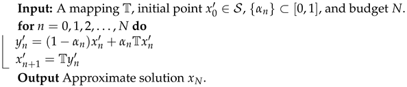We also conduct a weak $w^2$—stability analysis and obtain a sharp upper-bound estimate for the data dependence problem. The versatility of the proposed Algorithm 1 is further illustrated through two distinct applications. In the context of image deblurring modeled via wavelet-based ${\mathrm{\ell }}_1$ regularization, the algorithm was compared with widely used algorithms such as Picard, Mann [32], Ishikawa [33], Agarwal [34], and Normal S (Algorithm 2)  iteration algorithms on test images with different characteristics—namely, Airfield, Harbour, Kodim, and Clowns. The findings reveal that the Algorithm 1 achieves a rapid decrease in the objective function value, particularly within the first 20 iterations; exhibits a stable reduction in the Frobenius norm of successive iteration differences; and attains the highest PSNR values throughout all iterations. Visual results corroborate these quantitative findings, indicating that despite its simpler structure, the NS inertial-type algorithm offers a distinctly superior deblurring quality compared to its counterparts.

Parallel to these findings, in fractal pattern generation on the complex plane, the same set of fixed point iteration algorithms was employed to visualize Julia and Mandelbrot sets for functions of the form $\sin \left(z^n\right)+az+c$ using escape criteria. In this setting, the NS inertial-type iteration algorithm again demonstrated faster convergence, produced more extensive and orderly basins of attraction, and displayed more stable behavior in chaotic boundary regions relative to the other methods. Furthermore, inspired by recent developments, we employed a NS inertial-type iteration algorithm to obtain fractal visualizations, which proved to be even more effective than the Normal S iteration algorithm. These results collectively underscore the robustness and broad applicability of the proposed inertial framework across diverse computational domains.

The subsequent definitions and lemmas form the theoretical foundation for the results established in this work.

Definition 1

(See [35]). Let ${\left\{{\mathrm{\Phi }}_n^i\right\}}_{n=0}^{\infty }\subset \mathcal{S}$, for $i=1,2$, be two sequences. We say that these sequences are asymptotically equivalent if

$${\displaystyle \underset{n\to \infty }{\lim }}∥{\mathrm{\Phi }}_n^1-{\mathrm{\Phi }}_n^2∥=0.$$

Definition 2

(See [36]). Let $\mathbb{T}:\mathcal{S}\to \mathcal{S}$ be an operator with a fixed point $x_{*}\in Fix\left(\mathbb{T}\right)$, and let ${\left\{{\mathrm{\Phi }}_n^1\right\}}_{n=0}^{\infty }$ be an iteration sequence generated by

$$\left\{\begin{array}{c}{\mathrm{\Phi }}_0^1\in \mathcal{S},\\ {\mathrm{\Phi }}_{n+1}^1=\mathfrak{f}\left(\mathbb{T},{\mathrm{\Phi }}_n^1\right),n\in \mathbb{N}\cup \left\{0\right\},\end{array}\right.$$

where $\mathfrak{f}$ is a given function. Suppose that ${\left\{{\mathrm{\Phi }}_n^1\right\}}_{n=0}^{\infty }$ converges to $x_{*}$. The sequence ${\left\{{\mathrm{\Phi }}_n^1\right\}}_{n=0}^{\infty }$ is said to be weak $w^2$—stable w.r.t. $\mathbb{T}$ if, for every sequence ${\left\{{\mathrm{\Phi }}_n^2\right\}}_{n=0}^{\infty }\subset S$ that is asymptotically equivalent to ${\left\{{\mathrm{\Phi }}_n^1\right\}}_{n=0}^{\infty }$, the condition

$${\displaystyle \underset{n\to \infty }{\lim }}∥{\mathrm{\Phi }}_{n+1}^2-\mathfrak{f}\left(\mathbb{T},{\mathrm{\Phi }}_n^2\right)∥=0$$

implies

$${\displaystyle \underset{n\to \infty }{\lim }}{\mathrm{\Phi }}_n^2=x_{*}.$$

Remark 2.

In the literature, several concepts have been introduced to capture the numerical robustness of fixed point iterations. The strongest of these is $\mathbb{T}$—stability (see [37]), which requires that for any sequence ${\left\{{\mathrm{\Phi }}_n^2\right\}}_{n=0}^{\infty }$ (no matter how chosen), the implication ${\lim }_{n\to \infty }∥{\mathrm{\Phi }}_{n+1}^2-\mathfrak{f}\left(\mathbb{T},{\mathrm{\Phi }}_n^2\right)∥=0\Rightarrow {\lim }_{n\to \infty }{\mathrm{\Phi }}_n^2=x_{*}$ holds. A more realistic notion is weak stability (see [12]), where ${\left\{{\mathrm{\Phi }}_n^2\right\}}_{n=0}^{\infty }$ is required to be an approximate sequence of ${\left\{{\mathrm{\Phi }}_n^1\right\}}_{n=0}^{\infty }$; that is, $∥{\mathrm{\Phi }}_n^1-{\mathrm{\Phi }}_n^2∥\le \eta$ for some $\eta >0$ and for all sufficiently large n. An even weaker—and therefore more widely applicable—concept is weak $w^2$—stability, which only demands that ${\left\{{\mathrm{\Phi }}_n^2\right\}}_{n=0}^{\infty }$ be asymptotically equivalent to ${\left\{{\mathrm{\Phi }}_n^1\right\}}_{n=0}^{\infty }$, i.e., $∥{\mathrm{\Phi }}_n^1-{\mathrm{\Phi }}_n^2∥\to 0$ as $n\to \infty$. These notions form a strict hierarchy:

$$\mathbb{T}-\mathit{stable}\subset \mathit{weakly}\mathit{stable}\subset \mathit{weak}{w}^2-\mathit{stable}.$$

The weakest concept is the most natural for numerical computations, because in practice, errors often tend to zero (asymptotic equivalence) but may not be uniformly bounded from the outset. Hence, weak $w^2$—stability offers the mildest and most realistic condition under which an iteration algorithm can be considered numerically stable. This is precisely why we adopt it in the present work.

Lemma 1

(See [38]). Let ${\left\{{\mathrm{\Phi }}_n^i\right\}}_{n=0}^{\infty },i=1,2$ be two sequences such that ${\mathrm{\Phi }}_n^1,{\mathrm{\Phi }}_n^2\ge 0$, $\forall n\in \mathbb{N}$, ${\lim }_{n\to \infty }{\mathrm{\Phi }}_n^2=0$, and

$${\mathrm{\Phi }}_{n+1}^1\le \wp {\mathrm{\Phi }}_n^1+{\mathrm{\Phi }}_n^2,\forall n\in \mathbb{N}\cup \left\{0\right\},$$

in which $\wp \in \left[0,1\right)$ is a constant. It then holds that ${\lim }_{n\to \infty }{\mathrm{\Phi }}_n^1=0$.

2. Convergence Results for NS Inertial-Type Iteration Algorithm

Theorem 1.

Let the sequence $\left\{x_n\right\}$ be generated by the NS inertial-type iteration algorithm. If ${\sum }_{n=0}^{\infty }{ϵ}_n<\infty$, then ${\left\{x_n\right\}}_{n=1}^{\infty }$ converges strongly to the fixed point $x_{*}$ of an almost contraction mapping $\mathbb{T}:\mathcal{S}\to \mathcal{S}$ that satisfies condition (2) with a posteriori error estimate   

$$∥x_{n+1}-x_{*}∥\le {\lambda }^{2\left(n+1\right)}∥x_0-x_{*}∥+\lambda {\displaystyle \sum _{k=0}^n}{\lambda }^{2\left(n-k\right)}{ϵ}_k.$$

Proof. 

Since $\mathbb{T}$ is an almost contraction satisfying conditions (2), (3) and (4), it follows from (Berinde [3], Theorem 2) that $\mathbb{T}$ has a unique fixed point $x_{*}$, i.e., $\mathbb{T}{x}_{*}=x_{*}$. Substituting $x=x_{*}$ into condition (2) yields, for every $y\in \mathcal{S}$,

$$∥\mathbb{T}{x}_{*}-\mathbb{T}y∥\le \lambda ∥x_{*}-y∥+L∥x_{*}-\mathbb{T}{x}_{*}∥,$$

so that

$$∥\mathbb{T}{x}_{*}-\mathbb{T}y∥\le \lambda ∥x_{*}-y∥\left(\forall y\in \mathcal{S}\right).$$

(17)

Using the triangle inequality together with (17) and the definition of ${\theta }_n$, we obtain

$$\begin{array}{ccc}\hfill ∥y_n-x_{*}∥& \le & ∥\mathbb{T}{x}_n-\mathbb{T}{x}_{*}∥+{\theta }_n∥\mathbb{T}{x}_n-\mathbb{T}{x}_{n-1}∥\hfill \\ & \le & \lambda ∥x_n-x_{*}∥+{\theta }_n∥\mathbb{T}{x}_n-\mathbb{T}{x}_{n-1}∥.\hfill \end{array}$$

The construction of ${\theta }_n$ guarantees that ${\theta }_n∥\mathbb{T}{x}_n-\mathbb{T}{x}_{n-1}∥\le {ϵ}_n$ in both cases. Hence,

$$∥y_n-x_{*}∥\le \lambda ∥x_n-x_{*}∥+{ϵ}_n.$$

(18)

Since $x_{n+1}=\mathbb{T}{y}_n$, applying (17) with $y=y_n$ gives

$$∥x_{n+1}-x_{*}∥\le \lambda ∥y_n-x_{*}∥.$$

Combining this with (18) yields

$$∥x_{n+1}-x_{*}∥\le {\lambda }^2∥x_n-x_{*}∥+\lambda {ϵ}_n.$$

(19)

Iterating (19) produces a closed-form estimate. We claim that for every $n\ge 0$,

$$∥x_{n+1}-x_{*}∥\le {\left({\lambda }^2\right)}^{n+1}∥x_0-x_{*}∥+\lambda {\displaystyle \sum _{k=0}^n}{\left({\lambda }^2\right)}^{n-k}{ϵ}_k.$$

(20)

For $n=0$, (20) reduces to $∥x_1-x_{*}∥\le {\lambda }^2∥x_0-x_{*}∥+\lambda {ϵ}_0$, which is exactly (19). Assume that (20) holds for $n-1$. Then, using (19) and the induction hypothesis, we obtain

$$\begin{array}{ccc}\hfill ∥x_{n+1}-x_{*}∥& \le & {\lambda }^2∥x_n-x_{*}∥+\lambda {ϵ}_n\hfill \\ & \le & {\lambda }^2\left({\left({\lambda }^2\right)}^n∥x_0-x_{*}∥+\lambda {\displaystyle \sum _{k=0}^{n-1}}{\left({\lambda }^2\right)}^{n-1-k}{ϵ}_k\right)+\lambda {ϵ}_n\hfill \\ & =& {\left({\lambda }^2\right)}^{n+1}∥x_0-x_{*}∥+\lambda {\displaystyle \sum _{k=0}^{n-1}}{\left({\lambda }^2\right)}^{n-k}{ϵ}_k+\lambda {ϵ}_n\hfill \\ & =& {\left({\lambda }^2\right)}^{n+1}∥x_0-x_{*}∥+\lambda {\displaystyle \sum _{k=0}^n}{\left({\lambda }^2\right)}^{n-k}{ϵ}_k.\hfill \end{array}$$

The first term on the right-hand side of (20) clearly tends to zero because ${\lambda }^2<1$. It remains to prove that the second term,

$$S_n:=\lambda {\displaystyle \sum _{k=0}^n}{\left({\lambda }^2\right)}^{n-k}{ϵ}_k,$$

also converges to zero under the hypothesis ${\sum }_{k=0}^{\infty }{ϵ}_k<\infty$. To see this, fix an arbitrary $\epsilon >0$. Convergence of the series $\sum {ϵ}_k$ implies the existence of an integer N such that

$${\displaystyle \sum _{k=N}^{\infty }}{ϵ}_k<\epsilon .$$

(21)

For any $n>N$, we have

$${\displaystyle \sum _{k=0}^n}{\left({\lambda }^2\right)}^{n-k}{ϵ}_k={\displaystyle \sum _{k=0}^{N-1}}{\left({\lambda }^2\right)}^{n-k}{ϵ}_k+{\displaystyle \sum _{k=N}^n}{\left({\lambda }^2\right)}^{n-k}{ϵ}_k.$$

In the first sum, we have $n-k\ge n-N+1$; since the function $r\mapsto {\left({\lambda }^2\right)}^r$ is decreasing, ${\left({\lambda }^2\right)}^{n-k}\le {\left({\lambda }^2\right)}^{n-N+1}$ for all $k=0,1,\dots ,N-1$. Consequently,

$${\displaystyle \sum _{k=0}^{N-1}}{\left({\lambda }^2\right)}^{n-k}{ϵ}_k\le {\left({\lambda }^2\right)}^{n-N+1}{\displaystyle \sum _{k=0}^{N-1}}{ϵ}_k=:{\left({\lambda }^2\right)}^{n-N+1}M,$$

where M is a finite constant depending only on N. For the second sum, we use the trivial bound ${\left({\lambda }^2\right)}^{n-k}\le 1$ and then apply (21):

$${\displaystyle \sum _{k=N}^n}{\left({\lambda }^2\right)}^{n-k}{ϵ}_k\le {\displaystyle \sum _{k=N}^n}{ϵ}_k\le {\displaystyle \sum _{k=N}^{\infty }}{ϵ}_k<\epsilon .$$

Thus, for every $n>N$, we obtain

$${\displaystyle \sum _{k=0}^n}{\left({\lambda }^2\right)}^{n-k}{ϵ}_k\le {\left({\lambda }^2\right)}^{n-N+1}M+\epsilon .$$

Multiplying by $\lambda$ gives

$$S_n\le \lambda {\left({\lambda }^2\right)}^{n-N+1}M+\lambda \epsilon .$$

Since ${\lambda }^2<1$, it holds that ${\left({\lambda }^2\right)}^{n-N+1}M\to 0$ as $n\to \infty$. Hence, we can choose $N^{\prime }$ so that for all $n>N^{\prime }$, this factor is smaller than $\epsilon$ (since $\lambda$ is a constant, we may absorb it). Taking $n>\max \left\{N,N^{\prime }\right\}$ yields $S_n\le \lambda \epsilon +\lambda \epsilon =2\lambda \epsilon$; because $\epsilon$ was arbitrary, we conclude that ${\lim }_{n\to \infty }{S}_n=0$.

Returning to (20), we now have

$$∥x_{n+1}-x_{*}∥\le {\left({\lambda }^2\right)}^{n+1}∥x_0-x_{*}∥+S_n\to 0\mathrm{as}n\to \infty .$$

Therefore, $\left\{x_n\right\}$ converges strongly to the unique fixed point $x_{*}$, completing the proof.    □

It is important to note that the fulfillment of condition (2) ensures the uniqueness of the fixed point of the almost contraction mapping $\mathbb{T}$. In the subsequent result, we examine in further detail the convergence behaviors of the NS inertial-type iteration algorithm and Normal S iteration algorithm under the almost contraction framework when condition (2) is not met.

Theorem 2.

Let $\mathbb{T}$ be an almost contraction satisfying both inequalities (3) and (4), where $\lambda \in \left[0,1\right)$, $L\ge 0$, and $\lambda +L<1$. Suppose that $x_{*}$ is the unique fixed point of $\mathbb{T}$. Then:

(i) The sequence $\left\{x_n\right\}$ generated by the NS inertial-type iteration algorithm converges strongly to $x_{*}$, with the following a posteriori error estimates:

• Under condition (3):

  $$∥x_{n+1}-x_{*}∥\le {\rho }^{n+1}∥x_0-x_{*}∥+C{\displaystyle \sum _{j=0}^n}{\rho }^{n-j}{ϵ}_j,$$
  where $C=\lambda +L\left(\lambda +L\right)<1$, and $\rho =\lambda C/\left(1-L\right)<1$.
• Under condition (4):

  $$∥x_{n+1}-x_{*}∥\le d^{2\left(n+1\right)}∥x_0-x_{*}∥+d{\displaystyle \sum _{j=0}^n}{d}^{2\left(n-j\right)}{ϵ}_j,$$
  where $d=\lambda +L<1$.

(ii) The sequence $\left\{x_n^{\prime }\right\}$ generated by the Normal S iteration algorithm converges strongly to $x_{*}$, with the following a posteriori error estimates:

• Under condition (3):

  $$∥x_{n+1}^{\prime }-x_{*}∥\le \left({\displaystyle \prod _{j=0}^n}{\delta }_j\right)∥x_0^{\prime }-x_{*}∥,$$
  where ${\delta }_j=r\left[1-{\alpha }_j\left(1-r\right)\right]<1$, and $r=\lambda /\left(1-L\right)<1$.
• Under condition (4):

  $$∥x_{n+1}^{\prime }-x_{*}∥\le \left({\displaystyle \prod _{j=0}^n}{\delta }_j^{\prime }\right)∥x_0^{\prime }-x_{*}∥,$$
  where ${\delta }_j^{\prime }=d\left[1-{\alpha }_j\left(1-d\right)\right]<1$, and $d=\lambda +L<1$.

Proof. 

(i) We first consider the NS inertial-type iteration algorithm under condition (3). Since $x_{*}$ is the unique fixed point of $\mathbb{T}$, we have $\mathbb{T}{x}_{*}=x_{*}$. Using (3) with $x=y_n$ and $y=x_{*}$, we obtain

$$∥x_{n+1}-x_{*}∥=∥\mathbb{T}{y}_n-\mathbb{T}{x}_{*}∥\le \lambda ∥y_n-x_{*}∥+L∥x_{*}-\mathbb{T}{y}_n∥.$$

We now estimate the second term. Using again (3) with $x=x_{*}$, $y=y_n$, and $\mathbb{T}{x}_{*}=x_{*}$, we get

$$\begin{array}{ccc}\hfill ∥x_{*}-\mathbb{T}{y}_n∥& =& ∥\mathbb{T}{x}_{*}-\mathbb{T}{y}_n∥\hfill \\ & \le & \lambda ∥x_{*}-y_n∥+L∥y_n-\mathbb{T}{x}_{*}∥\hfill \\ & =& \left(\lambda +L\right)∥y_n-x_{*}∥.\hfill \end{array}$$

Substituting this into the previous inequality yields

$$∥x_{n+1}-x_{*}∥\le \left[\lambda +L\left(\lambda +L\right)\right]∥y_n-x_{*}∥.$$

Define

$$C:=\lambda +L\left(\lambda +L\right).$$

Next, we estimate $∥y_n-x_{*}∥$. By the definition of $y_n$ and the triangle inequality,

$$∥y_n-x_{*}∥=∥\mathbb{T}{x}_n+{\theta }_n\left(\mathbb{T}{x}_n-\mathbb{T}{x}_{n-1}\right)-x_{*}∥\le ∥\mathbb{T}{x}_n-x_{*}∥+{\theta }_n∥\mathbb{T}{x}_n-\mathbb{T}{x}_{n-1}∥.$$

Using (3) with $x=x_n$, $y=x_{*}$, and $\mathbb{T}{x}_{*}=x_{*}$, we have

$$∥\mathbb{T}{x}_n-x_{*}∥\le \lambda ∥x_n-x_{*}∥+L∥x_{*}-\mathbb{T}{x}_n∥,$$

which gives

$$∥\mathbb{T}{x}_n-x_{*}∥\le {\displaystyle \frac{\lambda }{1-L}}∥x_n-x_{*}∥.$$

Therefore,

$$∥y_n-x_{*}∥\le {\displaystyle \frac{\lambda }{1-L}}∥x_n-x_{*}∥+{\theta }_n∥\mathbb{T}{x}_n-\mathbb{T}{x}_{n-1}∥.$$

Set

$$t:={\displaystyle \frac{\lambda }{1-L}}.$$

Combining the above estimates, we obtain

$$∥x_{n+1}-x_{*}∥\le Ct∥x_n-x_{*}∥+C{\theta }_n∥\mathbb{T}{x}_n-\mathbb{T}{x}_{n-1}∥.$$

Since ${\theta }_n∥\mathbb{T}{x}_n-\mathbb{T}{x}_{n-1}∥\le {ϵ}_n$ for all n, it follows that

$$∥x_{n+1}-x_{*}∥\le \rho ∥x_n-x_{*}∥+C{ϵ}_n,$$

(22)

where

$$\rho :=Ct={\displaystyle \frac{\lambda C}{1-L}}.$$

Because $\lambda +L<1$, we have $C<1$ and $t<1$; hence, $\rho <1$. Iterating (22) by backward substitution gives, for every $n\ge 0$,

$$∥x_{n+1}-x_{*}∥\le {\rho }^{n+1}∥x_0-x_{*}∥+C{\displaystyle \sum _{j=0}^n}{\rho }^{n-j}{ϵ}_j.$$

This is the desired a posteriori error estimate under condition (3).

The remainder of the proof under condition (3) follows exactly the same pattern as the argument presented in the proof of Theorem 1.

The analysis under condition (4) proceeds in a similar fashion. Using (4) with appropriate choices of points yields the recurrence

$$∥x_{n+1}-x_{*}∥\le d^2∥x_n-x_{*}∥+d{\theta }_n∥\mathbb{T}{x}_n-\mathbb{T}{x}_{n-1}∥,\left(\forall n\ge 0\right),$$

where $d:=\lambda +L<1$. Employing again the bound ${\theta }_n∥\mathbb{T}{x}_n-\mathbb{T}{x}_{n-1}∥={ϵ}_n$ and iterating leads to the a posteriori estimate

$$∥x_{n+1}-x_{*}∥\le d^{2\left(n+1\right)}∥x_0-x_{*}∥+d{\displaystyle \sum _{j=0}^n}{d}^{2\left(n-j\right)}{ϵ}_j.$$

The same convergence argument as above (with $\rho$ replaced by $d^2$) shows that the right-hand side tends to zero, so strong convergence holds under condition (4) as well.

(ii) Using the Normal S iteration algorithm and the inequality in (3), we derive the following:

$$\begin{array}{ccc}\hfill ∥y_n^{\prime }-x_{*}∥& \le & \left(1-{\alpha }_n\right)∥x_n^{\prime }-x_{*}∥+{\alpha }_n∥\mathbb{T}{x}_n^{\prime }-x_{*}∥\hfill \\ & \le & \left[1-{\alpha }_n\left(1-{\displaystyle \frac{\lambda }{1-L}}\right)\right]∥x_n^{\prime }-x_{*}∥,\hfill \end{array}$$

(23)

and

$$∥x_{n+1}^{\prime }-x_{*}∥=∥\mathbb{T}{y}_n^{\prime }-\mathbb{T}{x}_{*}∥\le \lambda ∥y_n^{\prime }-x_{*}∥+L∥x_{*}-\mathbb{T}{y}_n^{\prime }∥,$$

which gives

$$∥x_{n+1}^{\prime }-x_{*}∥\le {\displaystyle \frac{\lambda }{1-L}}∥y_n^{\prime }-x_{*}∥.$$

(24)

Inserting (23) into (24) yields

$$∥x_{n+1}^{\prime }-x_{*}∥\le \tau \left[1-{\alpha }_n\left(1-\tau \right)\right]∥x_n^{\prime }-x_{*}∥,$$

where $\tau ={\displaystyle \frac{\lambda }{1-L}}<1$. Define ${\delta }_n:=\tau \left[1-{\alpha }_n\left(1-\tau \right)\right]$ for all $n\ge 0$. Since $\tau <1$ and ${\alpha }_n\in \left[0,1\right]$ for all $n\ge 0$, we have ${\delta }_n\le \tau <1$. Iterating the inequality yields the a posteriori error estimate

$$∥x_{n+1}^{\prime }-x_{*}∥\le \left({\displaystyle \prod _{j=0}^n}{\delta }_j\right)∥x_0^{\prime }-x_{*}∥.$$

Because each factor ${\delta }_j\le \tau <1$, the product tends to zero, so $\left\{x_n^{\prime }\right\}$ converges strongly to $x_{*}$.

Using the Normal S iteration algorithm and the inequality in (4), we derive the following:

$$\begin{array}{ccc}\hfill ∥y_n^{\prime }-x_{*}∥& \le & \left(1-{\alpha }_n\right)∥x_n^{\prime }-x_{*}∥+{\alpha }_n∥\mathbb{T}{x}_n^{\prime }-x_{*}∥\hfill \\ & \le & \left[1-{\alpha }_n\left(1-\left(\lambda +L\right)\right)\right]∥x_n^{\prime }-x_{*}∥,\hfill \end{array}$$

and

$$∥x_{n+1}^{\prime }-x_{*}∥=∥\mathbb{T}{y}_n^{\prime }-\mathbb{T}{x}_{*}∥\le \left(\lambda +L\right)∥y_n^{\prime }-x_{*}∥.$$

Combining these, we obtain

$$∥x_{n+1}^{\prime }-x_{*}∥\le d\left[1-{\alpha }_n\left(1-d\right)\right]∥x_n^{\prime }-x_{*}∥,$$

where $d=\lambda +L$. Set ${\delta }_n^{\prime }:=d\left[1-{\alpha }_n\left(1-d\right)\right]$ for all $n\ge 0$. Since $d<1$ and ${\alpha }_n\in \left[0,1\right]$ for all $n\ge 0$, we have ${\delta }_n\le d<1$. Iterating the inequality yields the a posteriori error estimate

$$∥x_{n+1}^{\prime }-x_{*}∥\le \left({\displaystyle \prod _{j=0}^n}{\delta }_j^{\prime }\right)∥x_0^{\prime }-x_{*}∥,$$

and again, the product converges to zero, proving strong convergence to $x_{*}$.    □

Theorem 3.

The following statements are equivalent:

(i) The sequence ${\left\{x_n^{\prime }-x_n\right\}}_{n=0}^{\infty }$ converges strongly to 0, and ${\left\{x_n^{\prime }\right\}}_{n=0}^{\infty }$ converges strongly to $x_{*}$.

(ii) The sequence ${\left\{x_n-x_n^{\prime }\right\}}_{n=0}^{\infty }$ converges strongly to 0, and ${\left\{x_n\right\}}_{n=0}^{\infty }$ converges strongly to $x_{*}$.

Proof. 

(i) Using condition (2) together with the definitions of the Normal S and NS inertial-type iteration algorithms, we estimate for all $n\in \mathbb{N}\cup \left\{0\right\}$:

$$\begin{array}{ccc}\hfill ∥x_{n+1}-x_{n+1}^{\prime }∥& \le & ∥\mathbb{T}{x}_{*}-\mathbb{T}{y}_n∥+∥\mathbb{T}{x}_{*}-\mathbb{T}{y}_n^{\prime }∥\hfill \\ & \le & \lambda ∥x_{*}-y_n∥+\lambda ∥x_{*}-y_n^{\prime }∥.\hfill \end{array}$$

Since

$$y_n=\mathbb{T}{x}_n+{\theta }_n\left(\mathbb{T}{x}_n-\mathbb{T}{x}_{n-1}\right),$$

we get

$$\begin{array}{ccc}\hfill ∥x_{*}-y_n∥& \le & ∥x_{*}-\mathbb{T}{x}_n∥+{\theta }_n∥\mathbb{T}{x}_n-\mathbb{T}{x}_{n-1}∥\hfill \\ & \le & \lambda ∥x_{*}-x_n∥+{ϵ}_n.\hfill \end{array}$$

On the other hand,

$$y_n^{\prime }=\left(1-{\alpha }_n\right)x_n^{\prime }+{\alpha }_n\mathbb{T}{x}_n^{\prime },$$

so

$$∥x_{*}-y_n^{\prime }∥\le \left(1-{\alpha }_n\right)∥x_{*}-x_n^{\prime }∥+{\alpha }_n∥x_{*}-\mathbb{T}{x}_n^{\prime }∥.$$

Using condition (2) together with $x=x_{*}$ and $y=x_n^{\prime }$, we have

$$∥x_{*}-\mathbb{T}{x}_n^{\prime }∥=∥\mathbb{T}{x}_{*}-\mathbb{T}{x}_n^{\prime }∥\le \lambda ∥x_{*}-x_n^{\prime }∥,$$

and therefore,

$$∥x_{*}-y_n^{\prime }∥\le \left[1-{\alpha }_n\left(1-\lambda \right)\right]∥x_{*}-x_n^{\prime }∥.$$

Combining these estimates yields

$$\begin{array}{ccc}\hfill ∥x_{n+1}-x_{n+1}^{\prime }∥& \le & {\lambda }^2∥x_{*}-x_n∥+\lambda \left[1-{\alpha }_n\left(1-\lambda \right)\right]∥x_{*}-x_n^{\prime }∥+\lambda {ϵ}_n\hfill \\ & \le & \lambda \left[1-{\alpha }_n\left(1-\lambda \right)\right]∥x_n-x_n^{\prime }∥+\lambda \left(1-{\alpha }_n\left(1-\lambda \right)+\lambda \right)∥x_{*}-x_n∥+\lambda {ϵ}_n.\hfill \end{array}$$

Since $1-{\alpha }_n\left(1-\lambda \right)<1$ for all $n\in \mathbb{N}\cup \left\{0\right\}$, we obtain

$${\mathrm{\Phi }}_{n+1}^1\le \wp {\mathrm{\Phi }}_n^1+{\mathrm{\Phi }}_n^2,$$

(25)

where

$${\mathrm{\Phi }}_n^1:=∥x_n-x_n^{\prime }∥\ge 0,\wp :=\lambda \in \left[0,1\right),$$

and

$${\delta }_n:=\lambda \left(1-{\alpha }_n\left(1-\lambda \right)+\lambda \right),{\mathrm{\Phi }}_n^2:={\delta }_n∥x_n-x_{*}∥+\lambda {ϵ}_n\ge 0.$$

Since ${\alpha }_n\in \left[0,1\right]$ for all $n\in \mathbb{N}\cup \left\{0\right\}$ and $\lambda \in \left[0,1\right)$, it follows that $\left\{{\delta }_n\right\}$ is bounded. Moreover, ${\sum }_{n=0}^{\infty }{ϵ}_n<\infty$ implies ${ϵ}_n\to 0$ as $n\to \infty$. Also by Theorem 1, we have ${\lim }_{n\to \infty }∥x_n-x_{*}∥=0$. Hence, ${\lim }_{n\to \infty }{\mathrm{\Phi }}_n^2=0$. An application of Lemma 1 then implies that ${\lim }_{n\to \infty }{\mathrm{\Phi }}_n^1=0$. Finally, by the triangle inequality,

$$∥x_n^{\prime }-x_{*}∥\le ∥x_n^{\prime }-x_n∥+∥x_n-x_{*}∥,$$

and since both terms on the right-hand side tend to zero, we conclude that

$${\displaystyle \underset{n\to \infty }{\lim }}∥x_n^{\prime }-x_{*}∥=0.$$

(ii) By employing an analogous argument using condition (2) in conjunction with the Normal S and NS inertial-type iteration algorithms, we likewise obtain for all $n\in \mathbb{N}\cup \left\{0\right\}$:

$$\begin{array}{ccc}\hfill ∥x_{n+1}^{\prime }-x_{n+1}∥& \le & ∥\mathbb{T}{y}_n^{\prime }-\mathbb{T}{y}_n∥\hfill \\ & \le & \lambda ∥x_{*}-y_n^{\prime }∥+\lambda ∥x_{*}-y_n∥\hfill \\ & \le & \lambda \left(1-{\alpha }_n\right)∥x_{*}-x_n^{\prime }∥+\lambda {\alpha }_n∥x_{*}-\mathbb{T}{x}_n^{\prime }∥\hfill \\ & & +\lambda ∥x_{*}-\mathbb{T}{x}_n∥+\lambda {\theta }_n∥\mathbb{T}{x}_n-\mathbb{T}{x}_{n-1}∥\hfill \\ & \le & \lambda \left[1-{\alpha }_n\left(1-\lambda \right)\right]∥x_{*}-x_n^{\prime }∥+{\lambda }^2∥x_{*}-x_n∥+\lambda {ϵ}_n\hfill \\ & \le & {\lambda }^2∥x_n^{\prime }-x_n∥+\lambda \left(\left[1-{\alpha }_n\left(1-\lambda \right)\right]+\lambda \right)∥x_{*}-x_n^{\prime }∥+\lambda {ϵ}_n.\hfill \end{array}$$

Since the subsequent steps mirror those in part (i), the details are omitted.    □

3. Stability and Data Dependence Results for NS Inertial-Type Iteration Algorithm

Theorem 4.

Let $\mathbb{T}$ and $\mathcal{S}$ be as specified in Theorem 1. Let $\left\{x_n\right\}$ be the sequence generated by the NS inertial-type iteration algorithm and $\left\{u_n\right\}\subset \mathcal{S}$ be a sequence asymptotically equivalent to $\left\{x_n\right\}$. Define a sequence $\left\{{\epsilon }_n\right\}$ in ${\mathbb{R}}^{+}$ by

$$\left\{\begin{array}{c}{\epsilon }_n=∥u_{n+1}-\mathbb{T}{v}_n∥,\hfill \\ v_n=\mathbb{T}{u}_n+{\mu }_n\left(\mathbb{T}{u}_n-\mathbb{T}{u}_{n-1}\right),n\ge 0,\end{array}\right.$$

(26)

where the sequence $\left\{{\mu }_n\right\}$ is defined by

$$0\le {\mu }_n\le \left\{\begin{array}{c}\min \left\{{\displaystyle \frac{n-1}{n+\eta -1}},{\displaystyle \frac{{ϵ}_n^{\prime }}{∥\mathbb{T}{u}_n-\mathbb{T}{u}_{n-1}∥}}\right\},\mathit{if}\mathbb{T}{u}_n\ne \mathbb{T}{u}_{n-1},\\ {\displaystyle \frac{n-1}{n+\eta -1}},\mathit{if}\mathbb{T}{u}_n=\mathbb{T}{u}_{n-1},\end{array}\right.$$

(27)

for some $\eta \ge 2$ and $\left\{{ϵ}_n^{\prime }\right\}\subset \left(0,\infty \right)$, with ${\sum }_{n=0}^{\infty }{ϵ}_n^{\prime }<\infty$. Then, the NS inertial-type iteration algorithm is weak $w^2$—stable with respect to $\mathbb{T}$.

Proof. 

Since $\left\{x_n\right\}$ converges strongly to $x_{*}$ by Theorem 1, it suffices to prove that under the given conditions, the asymptotically equivalent sequence $\left\{u_n\right\}$ also converges to $x_{*}$. From the definition of asymptotic equivalence, we have

$${\displaystyle \underset{n\to \infty }{\lim }}∥x_n-u_n∥=0.$$

Assume further that ${\lim }_{n\to \infty }{\epsilon }_n=0$. Using the NS inertial-type iteration algorithm together with (2), the definitions in (26) and the properties of ${\theta }_n$ and ${\mu }_n$, we obtain the following estimate:

$$\begin{array}{ccc}\hfill ∥u_{n+1}-x_{*}∥& \le & ∥u_{n+1}-x_{n+1}∥+∥x_{n+1}-x_{*}∥\hfill \\ & \le & ∥u_{n+1}-\mathbb{T}{v}_n∥+∥\mathbb{T}{v}_n-x_{n+1}∥+∥x_{n+1}-x_{*}∥\hfill \\ & =& {\epsilon }_n+∥\mathbb{T}{y}_n-\mathbb{T}{v}_n∥+∥x_{n+1}-x_{*}∥\hfill \\ & \le & {\epsilon }_n+\lambda ∥y_n-v_n∥+L∥y_n-\mathbb{T}{y}_n∥+∥x_{n+1}-x_{*}∥\hfill \\ & =& {\epsilon }_n+\lambda ∥\mathbb{T}{x}_n+{\theta }_n\left(\mathbb{T}{x}_n-\mathbb{T}{x}_{n-1}\right)-\mathbb{T}{u}_n-{\mu }_n\left(\mathbb{T}{u}_n-\mathbb{T}{u}_{n-1}\right)∥\hfill \\ & & +L∥y_n-\mathbb{T}{y}_n∥+∥x_{n+1}-x_{*}∥\hfill \\ & \le & {\epsilon }_n+\lambda ∥\mathbb{T}{x}_n-\mathbb{T}{u}_n∥+\lambda {\theta }_n∥\mathbb{T}{x}_n-\mathbb{T}{x}_{n-1}∥+\lambda {\mu }_n∥\mathbb{T}{u}_n-\mathbb{T}{u}_{n-1}∥\hfill \\ & & +L∥y_n-\mathbb{T}{y}_n∥+∥x_{n+1}-x_{*}∥\hfill \\ & \le & {\epsilon }_n+\lambda ∥\mathbb{T}{x}_n-\mathbb{T}{u}_n∥+\lambda {ϵ}_n+\lambda {ϵ}_n^{\prime }+L∥y_n-\mathbb{T}{y}_n∥+∥x_{n+1}-x_{*}∥\hfill \\ & \le & {\epsilon }_n+{\lambda }^2∥x_n-u_n∥+\lambda {ϵ}_n+\lambda {ϵ}_n^{\prime }+\lambda L∥x_n-\mathbb{T}{x}_n∥+L∥y_n-\mathbb{T}{y}_n∥+∥x_{n+1}-x_{*}∥\hfill \end{array}$$

Now, because $\left\{u_n\right\}\subset \mathcal{S}$ is asymptotically equivalent to $\left\{x_n\right\}$, we have ${\lim }_{n\to \infty }{\lambda }^2∥x_n-u_n∥=0$. From Theorem 1, we know that $x_n\to x_{*}$ implies that $∥x_n-\mathbb{T}{x}_n∥\to 0$ and $∥y_n-\mathbb{T}{y}_n∥\to 0$. The summability conditions ${\sum }_{n=0}^{\infty }{ϵ}_n<\infty$ and ${\sum }_{n=0}^{\infty }{ϵ}_n^{\prime }<\infty$ force ${ϵ}_n\to 0$ and ${ϵ}_n^{\prime }\to 0$. Taking the limit as $n\to \infty$ in the above inequality, and using ${\lim }_{n\to \infty }{ϵ}_n=0$, we obtain $u_n\to x_{*}$.    □

Theorem 5.

Let $\mathbb{T}:\mathcal{S}\to \mathcal{S}$ be an almost contraction satisfying (2) and $\tilde{\mathbb{T}}:\mathcal{S}\to \mathcal{S}$ be any mapping such that

$$∥\mathbb{T}x-\tilde{\mathbb{T}}x∥\le \epsilon \left(\forall x\in \mathcal{S}\right)$$

(28)

for some $\epsilon >0$. Suppose that $\left\{x_n\right\}$ is the sequence generated by the NS inertial-type iteration algorithm applied to $\mathbb{T}$ with parameter $\left\{{\theta }_n\right\}$ and a summable sequence $\left\{{ϵ}_n\right\}\subset \left(0,\infty \right)$, as defined in the algorithm. Let $\left\{{\tilde{x}}_n\right\}$ be the sequence generated by

Algorithm 3: NS inertial-type iteration algorithm for $\tilde{\mathbb{T}}$

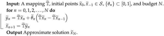Where the sequence $\left\{{\tilde{\theta }}_n\right\}$ is defined by

$$0\le {\tilde{\theta }}_n\le {\overline{\tilde{\theta }}}_n:=\left\{\begin{array}{c}\min \left\{{\displaystyle \frac{n-1}{n+\eta -1}},{\displaystyle \frac{{\widetilde{ϵ}}_n}{∥\tilde{\mathbb{T}}{\tilde{x}}_n-\tilde{\mathbb{T}}{\tilde{x}}_{n-1}∥}}\right\},\mathit{if}\tilde{\mathbb{T}}{\tilde{x}}_n\ne \tilde{\mathbb{T}}{\tilde{x}}_{n-1},\\ {\displaystyle \frac{n-1}{n+\eta -1}},\mathit{if}\tilde{\mathbb{T}}{\tilde{x}}_n=\tilde{\mathbb{T}}{\tilde{x}}_{n-1},\end{array}\right.$$

(29)

for some $\eta \ge 2$ and $\left\{{\widetilde{ϵ}}_n\right\}\subset \left(0,\infty \right)$, with ${\sum }_{n=0}^{\infty }{\widetilde{ϵ}}_n<\infty$. If ${\lim }_{n\to \infty }{\tilde{x}}_n={\tilde{x}}_{*}$ and ${\tilde{x}}_{*}=\tilde{\mathbb{T}}{\tilde{x}}_{*}$, then the following error estimate holds:

$$∥x_{*}-{\tilde{x}}_{*}∥\le {\displaystyle \frac{\epsilon }{1-\lambda }},$$

(30)

where $x_{*}$ denotes the unique fixed point of $\mathbb{T}$.

Proof. 

Using the definitions of the Algorithms 2 and 3 together with condition (2) and the properties of ${\theta }_n$ and ${\tilde{\theta }}_n$, we obtain

$$∥x_{n+1}-{\tilde{x}}_{n+1}∥\le ∥\mathbb{T}{y}_n-\mathbb{T}{\tilde{y}}_n∥+∥\mathbb{T}{\tilde{y}}_n-\tilde{\mathbb{T}}{\tilde{y}}_n∥.$$

Applying conditions (2) and (28), it follows that

$$∥x_{n+1}-{\tilde{x}}_{n+1}∥\le \lambda ∥y_n-{\tilde{y}}_n∥+L∥y_n-\mathbb{T}{y}_n∥+ϵ.$$

From the definition of $y_n$ and ${\tilde{y}}_n$, we have

$$∥y_n-{\tilde{y}}_n∥\le ∥\mathbb{T}{x}_n-\tilde{\mathbb{T}}{\tilde{x}}_n∥+{\theta }_n∥\mathbb{T}{x}_n-\mathbb{T}{x}_{n-1}∥+{\tilde{\theta }}_n∥\tilde{\mathbb{T}}{\tilde{x}}_n-\tilde{\mathbb{T}}{\tilde{x}}_{n-1}∥.$$

Hence,

$$\begin{array}{ccc}\hfill ∥x_{n+1}-{\tilde{x}}_{n+1}∥& \le & \lambda ∥\mathbb{T}{x}_n-\tilde{\mathbb{T}}{\tilde{x}}_n∥+\lambda {\theta }_n∥\mathbb{T}{x}_n-\mathbb{T}{x}_{n-1}∥\hfill \\ & & +\lambda {\tilde{\theta }}_n∥\tilde{\mathbb{T}}{\tilde{x}}_n-\tilde{\mathbb{T}}{\tilde{x}}_{n-1}∥+L∥y_n-\mathbb{T}{y}_n∥+ϵ.\hfill \end{array}$$

Using again conditions (2) and (28), we obtain

$$\begin{array}{ccc}\hfill ∥x_{n+1}-{\tilde{x}}_{n+1}∥& \le & \lambda ∥\mathbb{T}{x}_n-\mathbb{T}{\tilde{x}}_n∥+\lambda \epsilon +\lambda {ϵ}_n+\lambda {\widetilde{ϵ}}_n+L∥y_n-\mathbb{T}{y}_n∥+\epsilon \hfill \\ & \le & {\lambda }^2∥x_n-{\tilde{x}}_n∥+\lambda L∥x_n-\mathbb{T}{x}_n∥+L∥y_n-\mathbb{T}{y}_n∥\hfill \\ & & +\lambda \left({ϵ}_n+{\widetilde{ϵ}}_n\right)+\left(\lambda +1\right)\epsilon .\hfill \end{array}$$

(31)

Define $a_n:=∥x_n-{\tilde{x}}_n∥$ and $c_n:=\lambda L∥x_n-\mathbb{T}{x}_n∥+L∥y_n-\mathbb{T}{y}_n∥+\lambda \left({ϵ}_n+{\widetilde{ϵ}}_n\right)$ for all $n\ge 0$. Then, (31) becomes

$$a_{n+1}\le {\lambda }^2{a}_n+\left(\lambda +1\right)\epsilon +c_n\left(\forall n\ge 0\right).$$

(32)

It follows from Theorem 1 that $x_n\to x_{*}$ and $y_n\to x_{*}$ as $n\to \infty$; therefore, $∥x_n-\mathbb{T}{x}_n∥\to 0$ and $∥y_n-\mathbb{T}{y}_n∥\to 0$ as $n\to \infty$. Since ${\sum }_{n=0}^{\infty }{ϵ}_n<\infty$ and ${\sum }_{n=0}^{\infty }{\widetilde{ϵ}}_n<\infty$, we also have ${ϵ}_n\to 0$ and ${\widetilde{ϵ}}_n\to 0$ as $n\to \infty$. Consequently, $c_n\to 0$ as $n\to \infty$. Taking the limit superior in (32) and using that ${\mathrm{lim\; sup}}_{n\to \infty }{a}_{n+1}={\mathrm{lim\; sup}}_{n\to \infty }{a}_n$, we obtain

$${\displaystyle \underset{n\to \infty }{\mathrm{lim\; sup} }}{a}_{n+1}\le {\lambda }^2{\displaystyle \underset{n\to \infty }{\mathrm{lim\; sup} }}{a}_n+\left(\lambda +1\right)\epsilon ,$$

i.e., $\left(1-{\lambda }^2\right){\mathrm{lim\; sup}}_{n\to \infty }{a}_n\le \left(\lambda +1\right)\epsilon$. Hence,

$${\displaystyle \underset{n\to \infty }{\mathrm{lim\; sup} }}{a}_n\le {\displaystyle \frac{\left(\lambda +1\right)\epsilon }{1-{\lambda }^2}}.$$

Since $x_n\to x_{*}$ and ${\tilde{x}}_n\to {\tilde{x}}_{*}$ as $n\to \infty$, it follows that $a_n\to ∥x_{*}-{\tilde{x}}_{*}∥$; therefore, its limit superior coincides with its limit. Passing to the limit yields

$$∥x_{*}-{\tilde{x}}_{*}∥\le {\displaystyle \frac{\left(\lambda +1\right)\epsilon }{1-{\lambda }^2}}={\displaystyle \frac{\epsilon }{1-\lambda }}.$$

   □

4. A Comparative Study of the Computational Performance of Various Algorithms in Image Restoration Problems

In this section, the effectiveness of the NS inertial-type iteration algorithm, developed and analyzed in the previous sections, is evaluated through a comparative study on the classical image deblurring problem.

Image deblurring is a fundamental task in image processing, with applications in areas such as medical imaging, astronomy, satellite imaging, biometrics, and industrial inspection. The observed images are often degraded by blur and noise due to factors such as camera motion, defocusing, and atmospheric distortions.

Mathematically, image deblurring is formulated as an inverse problem, which is typically ill-posed, meaning that small perturbations in the data can lead to large reconstruction errors. To overcome this issue, regularization techniques are employed. In particular, ${\mathrm{\ell }}_1$-norm regularization is widely used due to its ability to promote sparsity.

Wavelet transforms offer an effective framework for sparsity-based regularization by providing multiresolution representations of images. Since natural images can often be well approximated by a few significant wavelet coefficients, wavelet-based ${\mathrm{\ell }}_1$-regularized models are especially suitable for image deblurring.

To ensure a precise and reproducible formulation, we explicitly define the forward model used in the image deblurring problem. The blur is generated by a spatially invariant convolution operator with a Gaussian point spread function. Specifically, the blur kernel is taken as

$$K=\mathtt{psfGauss}\left(\right[9,9],5),$$

and the convolution is applied with symmetric boundary conditions.

The operator A is modeled as a linear blurring operator corresponding to a spatially invariant convolution process, that is,

$$Ax=K\ast x,$$

where K denotes the blur kernel, and ∗ represents the two-dimensional discrete convolution. In the numerical experiments, the image is processed channel-wise, i.e., the red, green, and blue components are blurred separately.

Moreover, the regularization is imposed in the wavelet domain. Let W denote the discrete wavelet transform (DWT) and $W^{-1}$ its inverse. If x denotes the unknown image, then the ${\mathrm{\ell }}_1$-regularized inverse problem is written as

$${\displaystyle \underset{x}{\min }}{F}_{\mathrm{deb}}\left(x\right)={\parallel Ax-b\parallel }_2^2+\lambda {\parallel Wx\parallel }_1,$$

(33)

where b is the observed blurred and noisy image, and $\lambda >0$ is the regularization parameter.

Here, $f\left(x\right)={\parallel Ax-b\parallel }_2^2$ is differentiable and convex, while $g\left(x\right)={\lambda \parallel Wx\parallel }_1$ is convex but non-smooth. Since W is orthogonal, the proximal operator associated with the ${\mathrm{\ell }}_1$-term reduces to a soft-thresholding step in the wavelet domain. More precisely,

$${\mathrm{prox}}_{{\lambda t\parallel W·\parallel }_1}\left(u\right)=W^{-1}\left(\mathrm{sgn}\left(Wu\right)\max \left\{\right|Wu|-\lambda t,0\}\right),$$

which is applied component-wise.

Using this, the fixed point mapping $\mathbb{T}$ common to all iteration algorithms is defined as

$$\mathbb{T}\left(u\right):=W^{-1}\left(\mathrm{sgn}\left(W\left(v\right)\right)\max \left\{\right|W\left(v\right)|-\lambda t,0\}\right),v=u-t\nabla f\left(u\right),$$

where

$$\nabla f\left(u\right)=2A^{\top }(Au-b).$$

The adjoint operator $A^{\top }$ corresponds to convolution with the flipped kernel under reflexive boundary conditions. The Lipschitz constant of $\nabla f$ is

$$L=2\parallel A^{\top }A\parallel ,$$

and the step size is chosen accordingly.

This formulation establishes a direct connection with the classical ISTA framework and allows all algorithms to be interpreted within a unified fixed point setting.

We now explicitly present all iteration algorithms used in the comparison. All algorithms are implemented using the same operator $\mathbb{T}$, ensuring a fair and consistent comparison.

(i)

Picard-I iteration (ISTA):

$$u_{n+1}=\mathbb{T}\left(u_n\right).$$

(ii)

Mann-I iteration:

$$u_{n+1}=(1-{\alpha }_n)u_n+{\alpha }_n\mathbb{T}\left(u_n\right),{\alpha }_n\in (0,1).$$

(iii)

Ishikawa-I iteration:

$$\begin{array}{cc}\hfill y_n& =(1-{\beta }_n)u_n+{\beta }_n\mathbb{T}\left(u_n\right),\hfill \\ \hfill u_{n+1}& =(1-{\alpha }_n)u_n+{\alpha }_n\mathbb{T}\left(y_n\right),\hfill \end{array}{\alpha }_n,{\beta }_n\in (0,1).$$

(iv)

Agarwal-I iteration:

$$\begin{array}{cc}\hfill y_n& =(1-{\beta }_n)u_n+{\beta }_n\mathbb{T}\left(u_n\right),\hfill \\ \hfill u_{n+1}& =(1-{\alpha }_n)\mathbb{T}\left(u_n\right)+{\alpha }_n\mathbb{T}\left(y_n\right).\hfill \end{array}$$

(v)

NS-I iteration:

$$\begin{array}{cc}\hfill y_n& =(1-{\beta }_n)u_n+{\beta }_n\mathbb{T}\left(u_n\right),\hfill \\ \hfill u_{n+1}& =\mathbb{T}\left(y_n\right).\hfill \end{array}$$

(vi)

NS-inert.-I (proposed method):

$$\begin{array}{cc}\hfill y_n& =T\left(u_n\right)+{\theta }_n(T\left(u_n\right)-T\left(u_{n-1)}\right),\hfill \\ \hfill u_{n+1}& =\mathbb{T}\left(y_n\right),\hfill \end{array}$$

where ${\theta }_n$ is the inertial parameter.

The numerical experiments are carried out using the following parameter choices:

• Blur kernel: A Gaussian point spread function of size $9\times 9$ with standard deviation $\sigma =5$ is used.
• Noise level: Additive Gaussian noise with magnitude ${10}^{-3}$ is added to the blurred image.
• Random seed: The random number generator is initialized with seed 314.
• Boundary conditions: Reflexive (symmetric) boundary conditions are employed.
• Maximum number of iterations: $\mathtt{MAXITER}=100$.
• Step size: The step size is chosen as

  $$t={\displaystyle \frac{1}{L}},$$

  where $L={2\max \left|S\right|}^2$ is the Lipschitz constant computed from the spectral representation of the operator, and S denotes the Fourier representation of the convolution kernel.
• Iteration parameters: The control sequences are selected as

  $${\alpha }_n={\beta }_n={\displaystyle \frac{1}{k^{10}+1}}.$$
• Initialization: The algorithm is initialized with the observed image, i.e.,

  $$u_0=b.$$
• Frobenius norm error:

  $$\parallel u_n-u^{*}{\parallel }_F,$$
• Peak Signal-to-Noise Ratio (PSNR):

  $$\mathrm{PSNR}(u_n,u^{*})=10{\log }_{10}\left({\displaystyle \frac{MA{X}^2}{\mathrm{MSE}}}\right),$$

  where $u^{*}$ denotes the reference image and $MAX=255$ for 8-bit images.

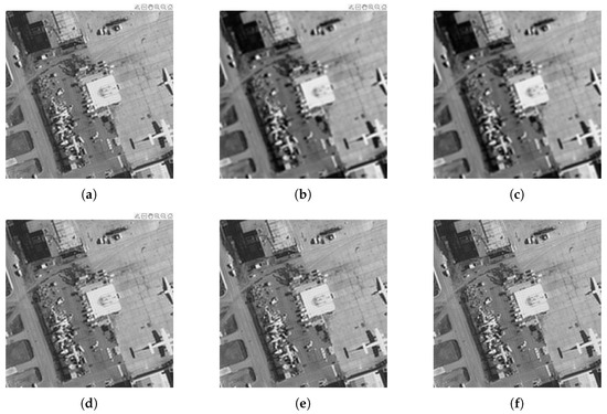
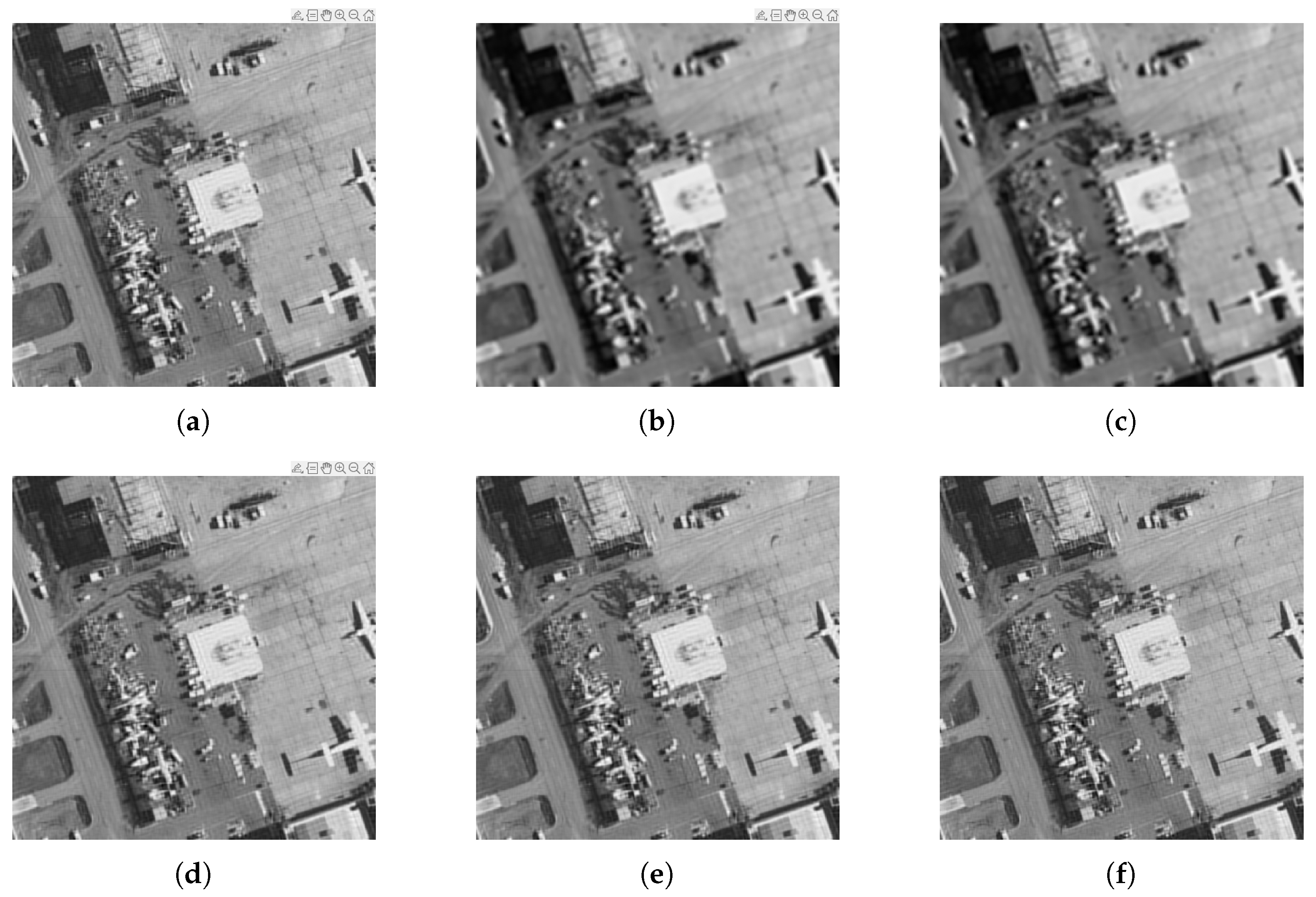
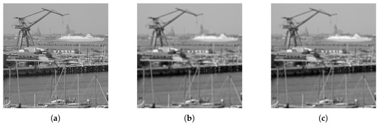
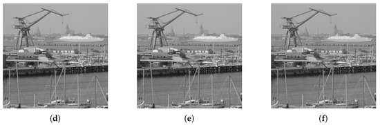
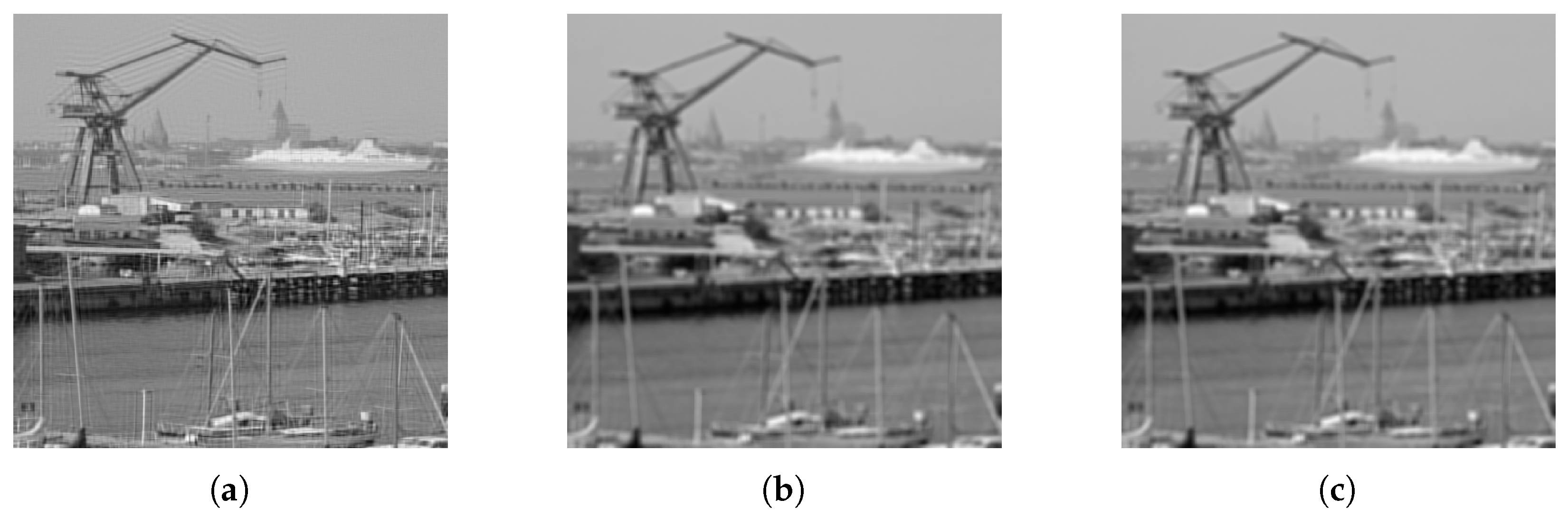
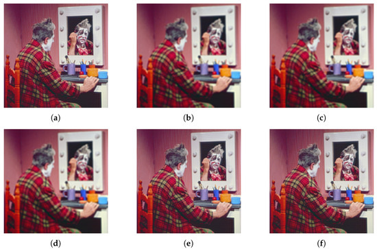
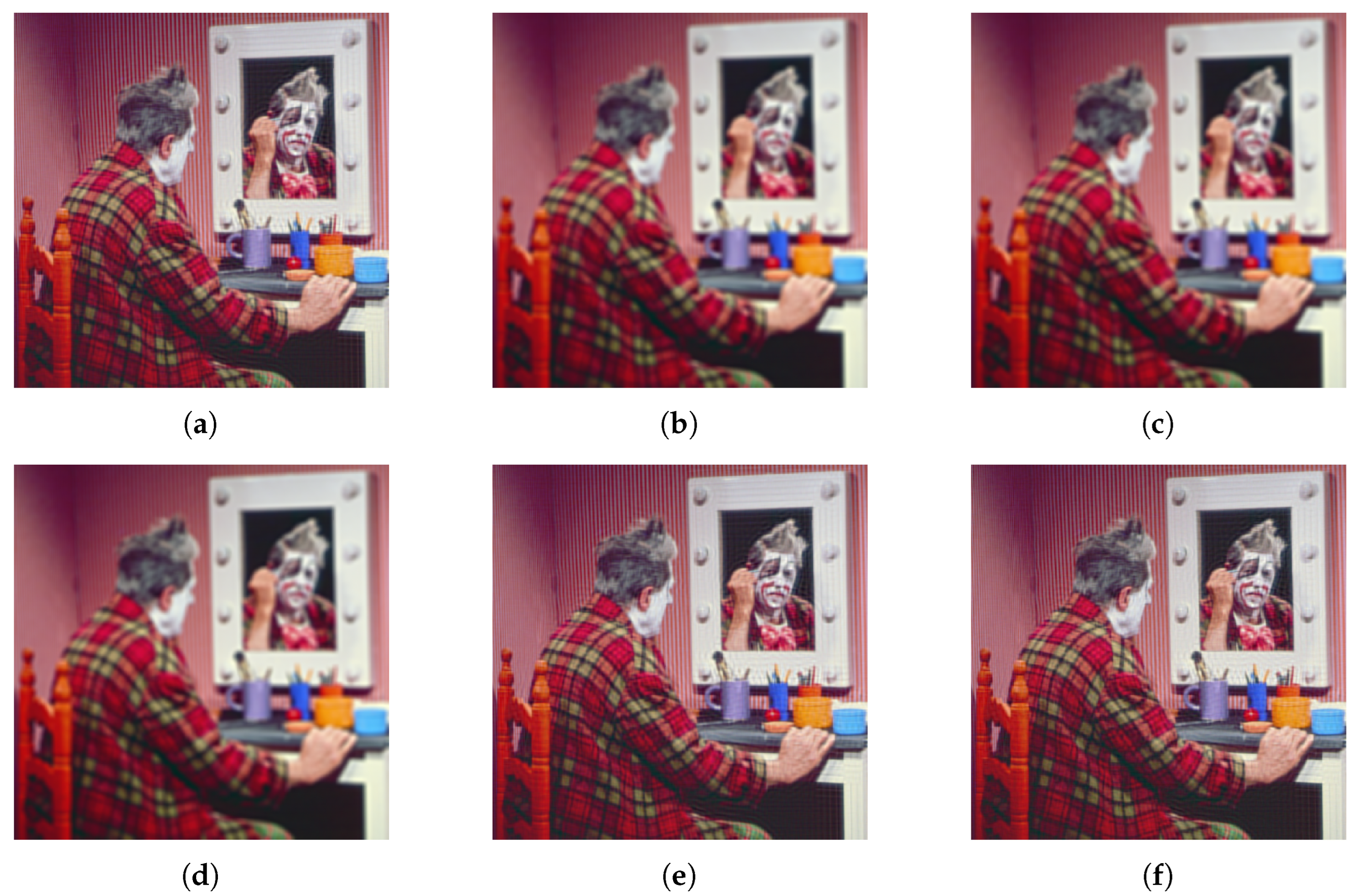
• The original test images and their blurred versions obtained using the same blurring operator are presented in Figure 1 and Figure 2, respectively. Grayscale images Airfield and Harbour and color images Kodim and Clowns are used as benchmark datasets. After applying the same blurring operator to all images, the deblurring is performed using the Picard-I (ISTA), Mann-I, Ishikawa-I, Agarwal-I, NS-I, and NS-Inert.-I algorithms, and their results are compared.

Figure 1. The original test images. (a) Airfield; (b) Harbour; (c) Kodim; (d) Clowns.

Figure 1. The original test images. (a) Airfield; (b) Harbour; (c) Kodim; (d) Clowns.

Figure 2. The blurred versions of all test images obtained by applying the same blurring operator. (a) Airfield; (b) Harbour; (c) Kodim; (d) Clowns.

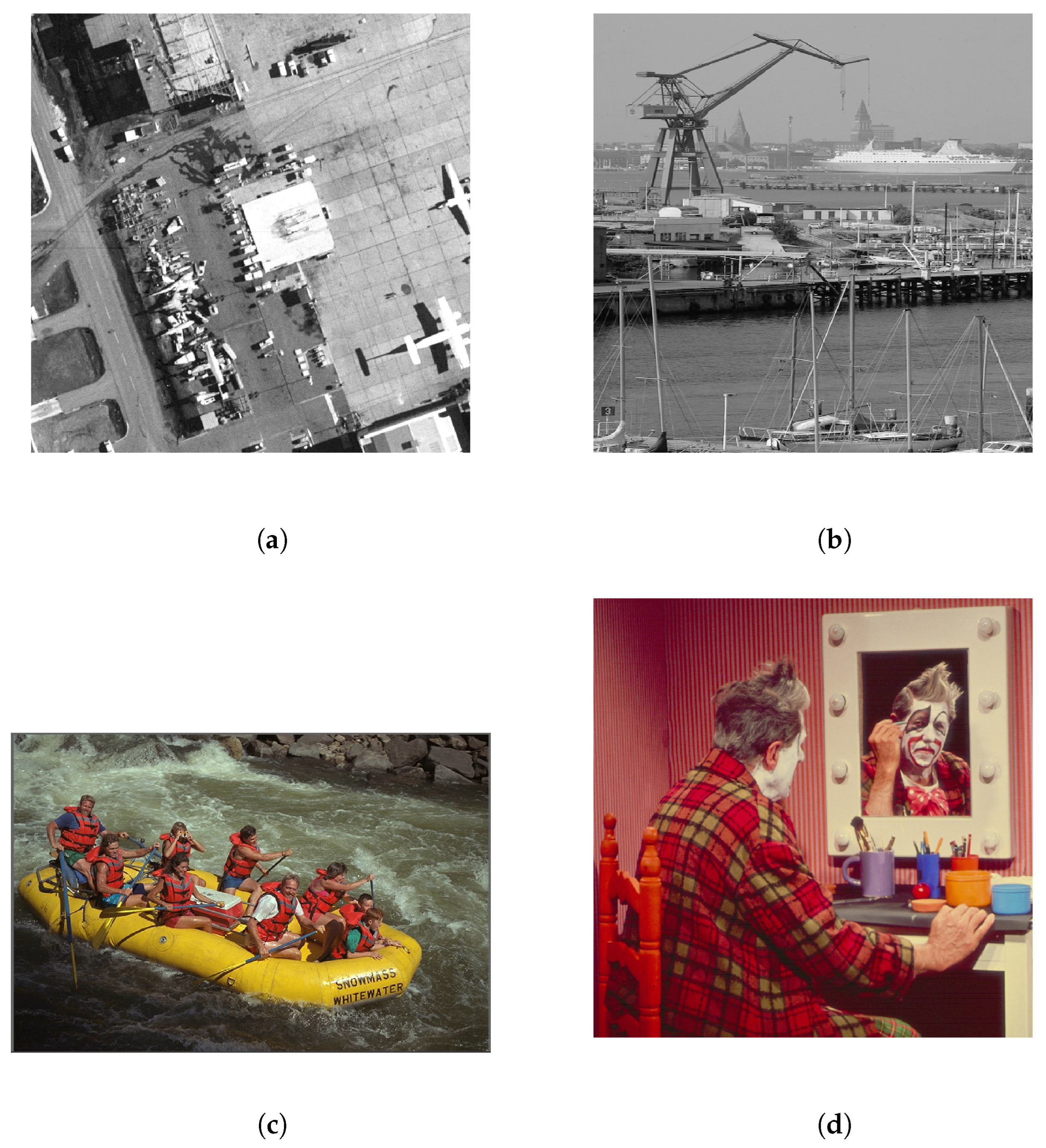
Figure 2. The blurred versions of all test images obtained by applying the same blurring operator. (a) Airfield; (b) Harbour; (c) Kodim; (d) Clowns.

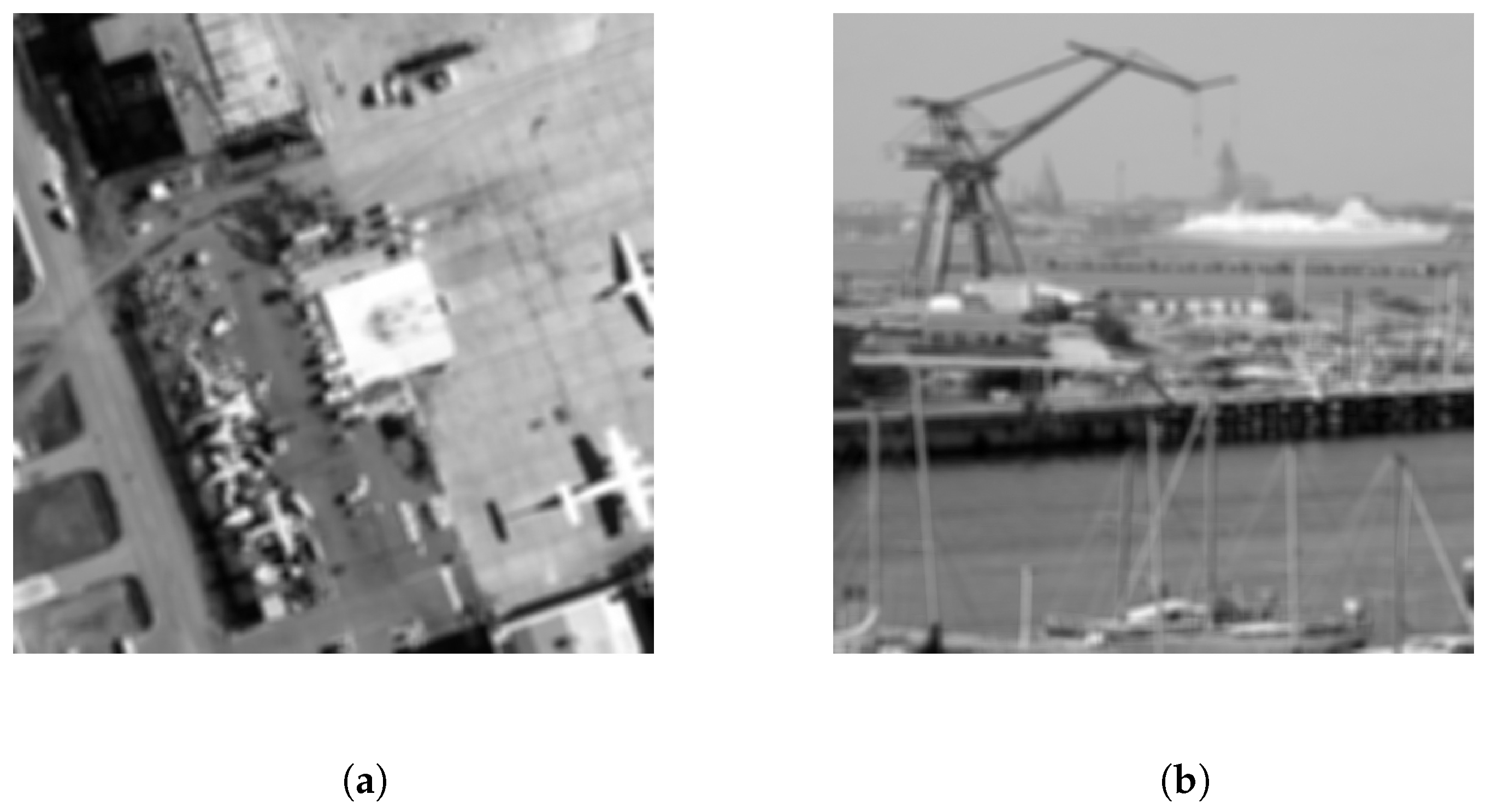
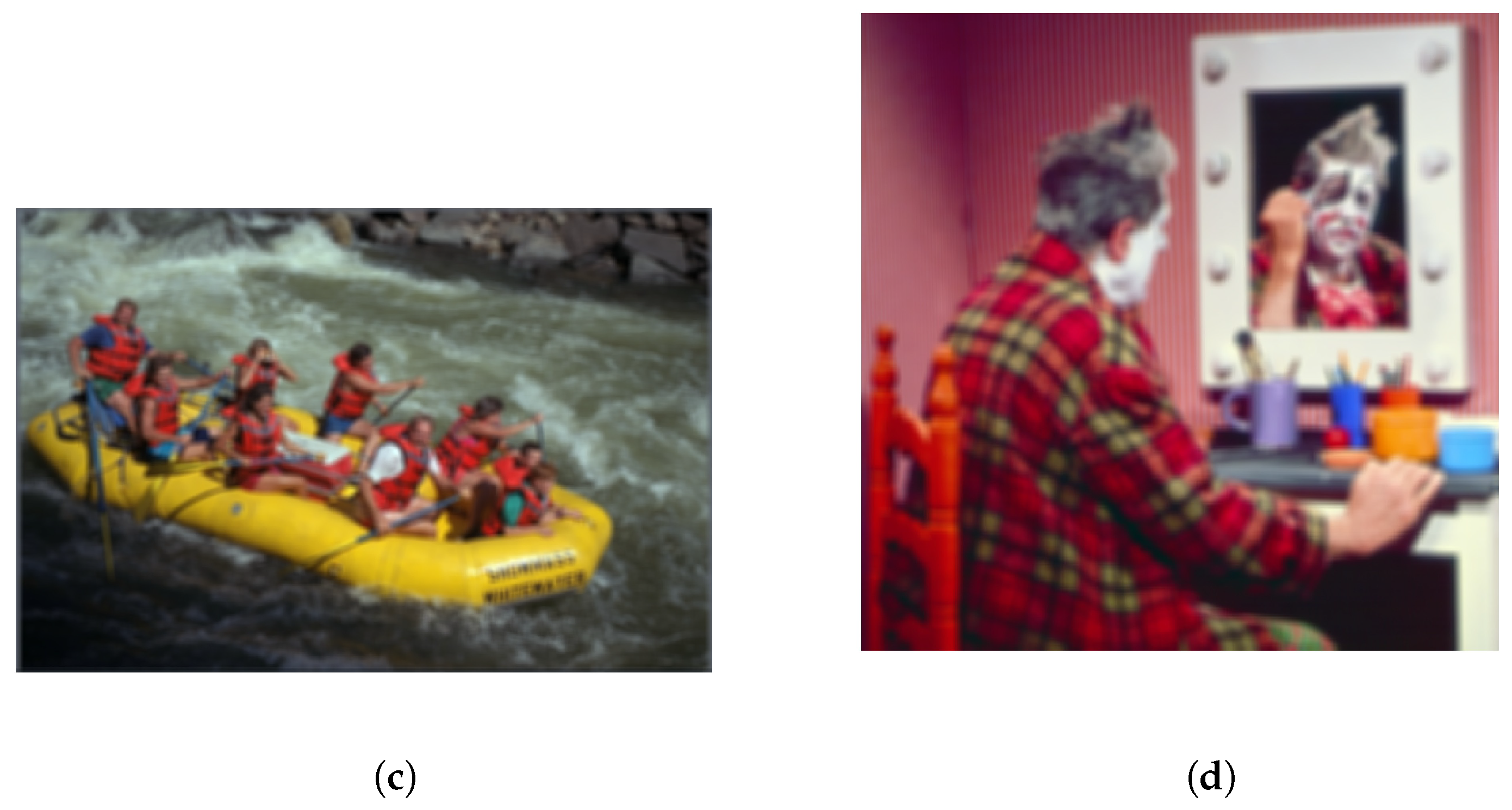
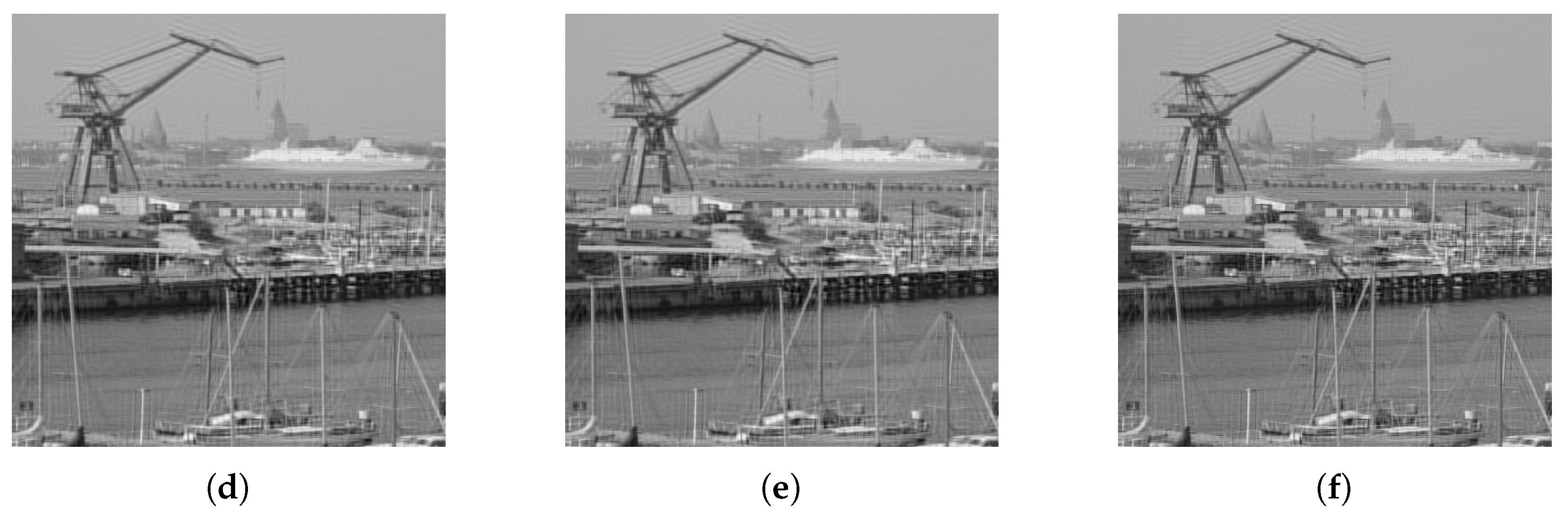
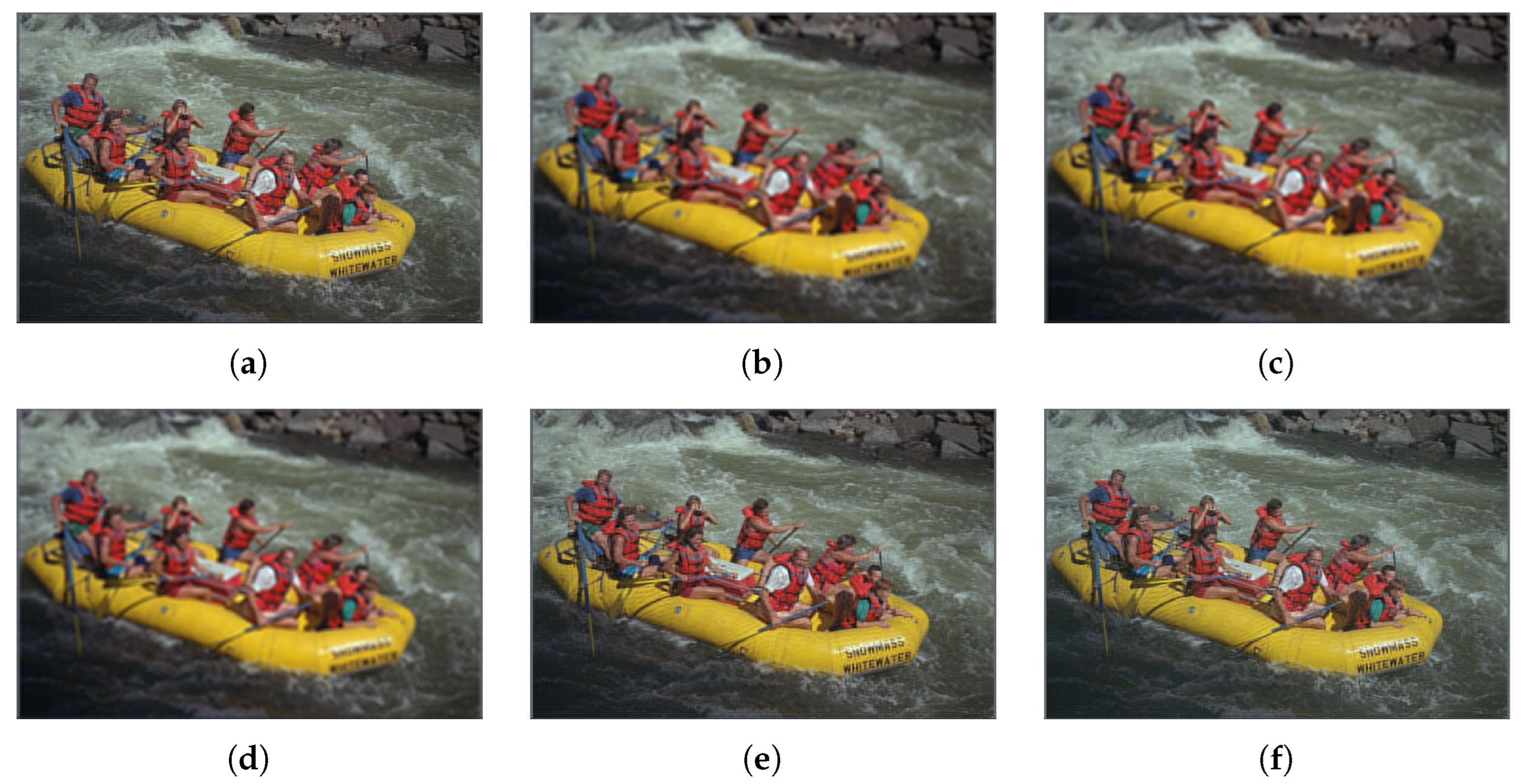
Figure 3, Figure 4, Figure 5 and Figure 6 display the deblurred results of all algorithms in a unified comparative layout. The visual comparisons clearly demonstrate that the NS-Inert.-I algorithm provides the best reconstruction quality for every test image.

Figure 3. Comparison of the deblurred images obtained using (a) Picard-I; (b) Mann-I; (c) Ishikawa-I; (d) Agarwal-I; (e) NS-I; (f) NS-Inert.-I.

Figure 4. Comparison of the deblurred images obtained using (a) Picard-I; (b) Mann-I; (c) Ishikawa-I; (d) Agarwal-I; (e) NS-I; (f) NS-Inert.-I.

Figure 5. Comparison of the deblurred images obtained using (a) Picard-I; (b) Mann-I; (c) Ishikawa-I; (d) Agarwal-I; (e) NS-I; (f) NS-Inert.-I.

Figure 6. Comparison of the deblurred images obtained using (a) Picard-I; (b) Mann-I; (c) Ishikawa-I; (d) Agarwal-I; (e) NS-I; (f) NS-Inert.-I.

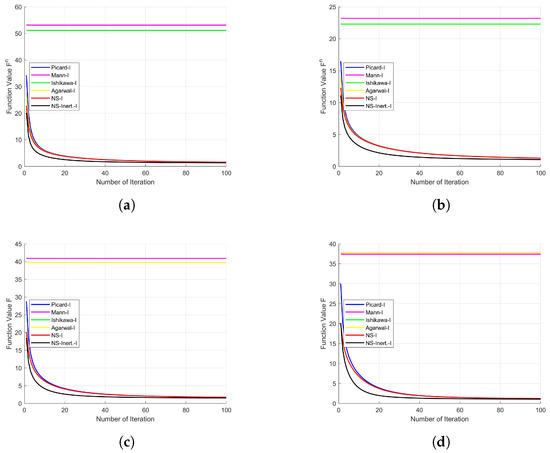
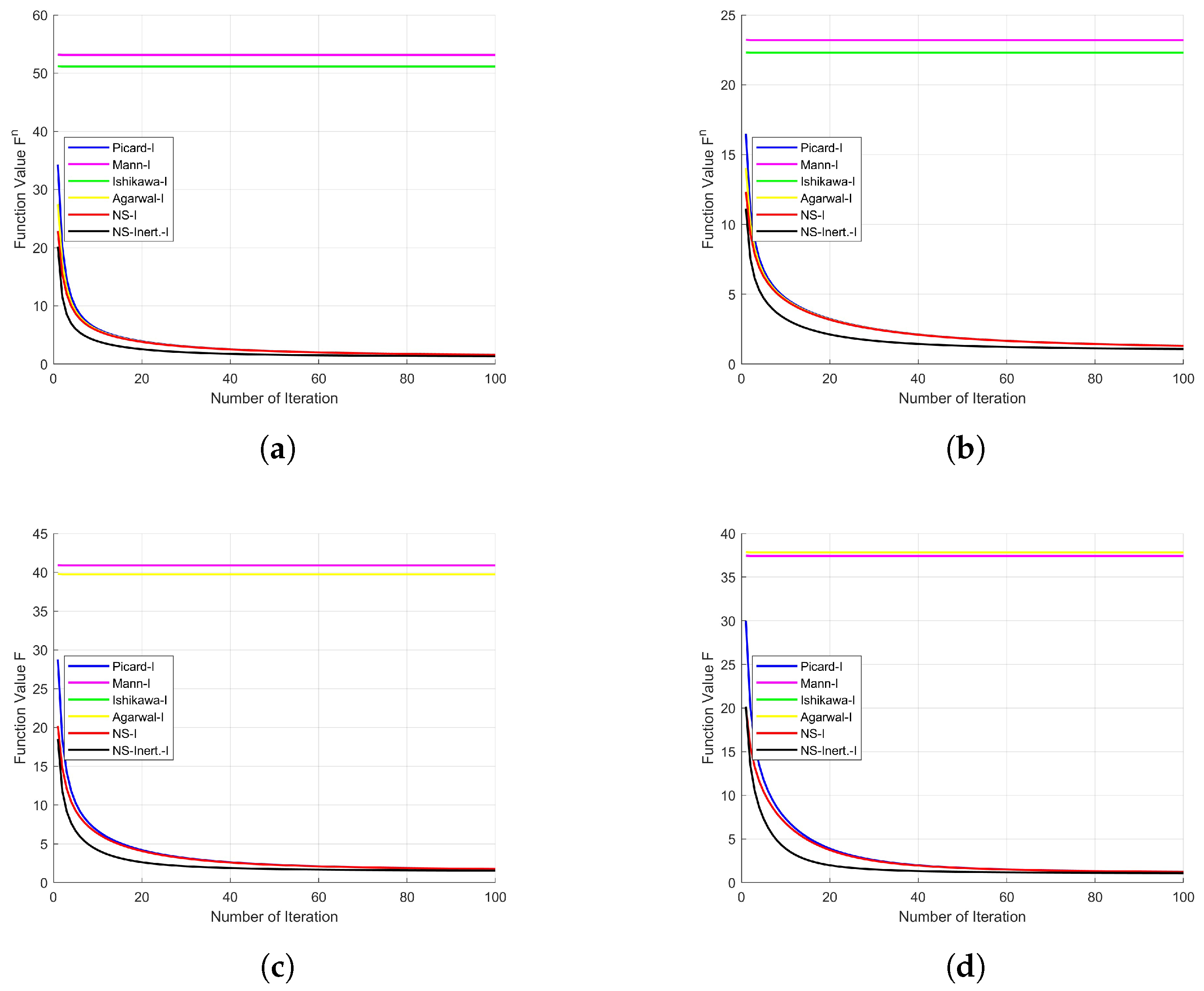
For a detailed analysis of the algorithms’ convergence behavior, the objective function values, the Frobenius norms of successive iteration differences, and the PSNR values were evaluated at each iteration.

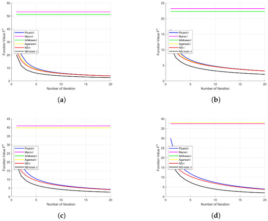
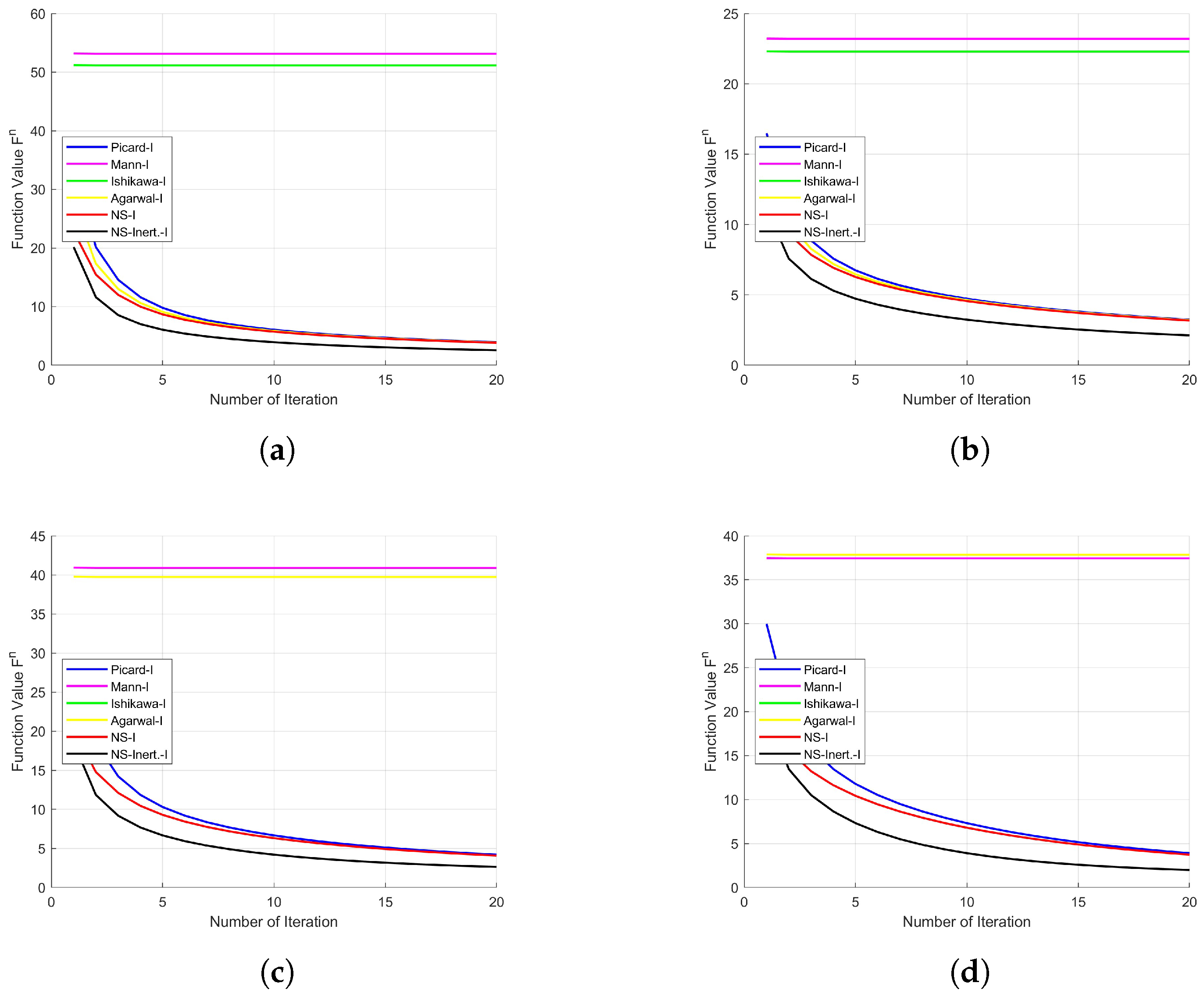
Figure 7 and Figure 8 show that the NS-Inert.-I algorithm achieved a notably rapid reduction in the objective function values during the first 20 iterations and preserved this superior performance across the remaining iterations.

Figure 7. Iteration-wise changes of the objective function $F^n$ during the first 100 steps for the images (a) Airfield; (b) Harbour; (c) Kodim; (d) Clowns.

Figure 8. Changes in the objective function $F^n$ over the first 20 iterations for images (a) Airfield; (b) Harbour; (c) Kodim; (d) Clowns.

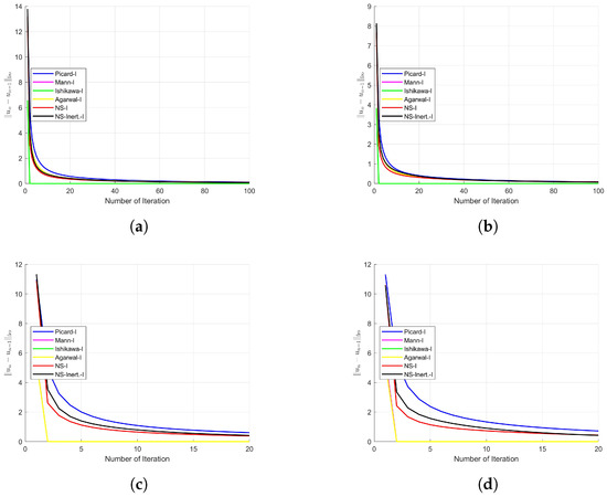
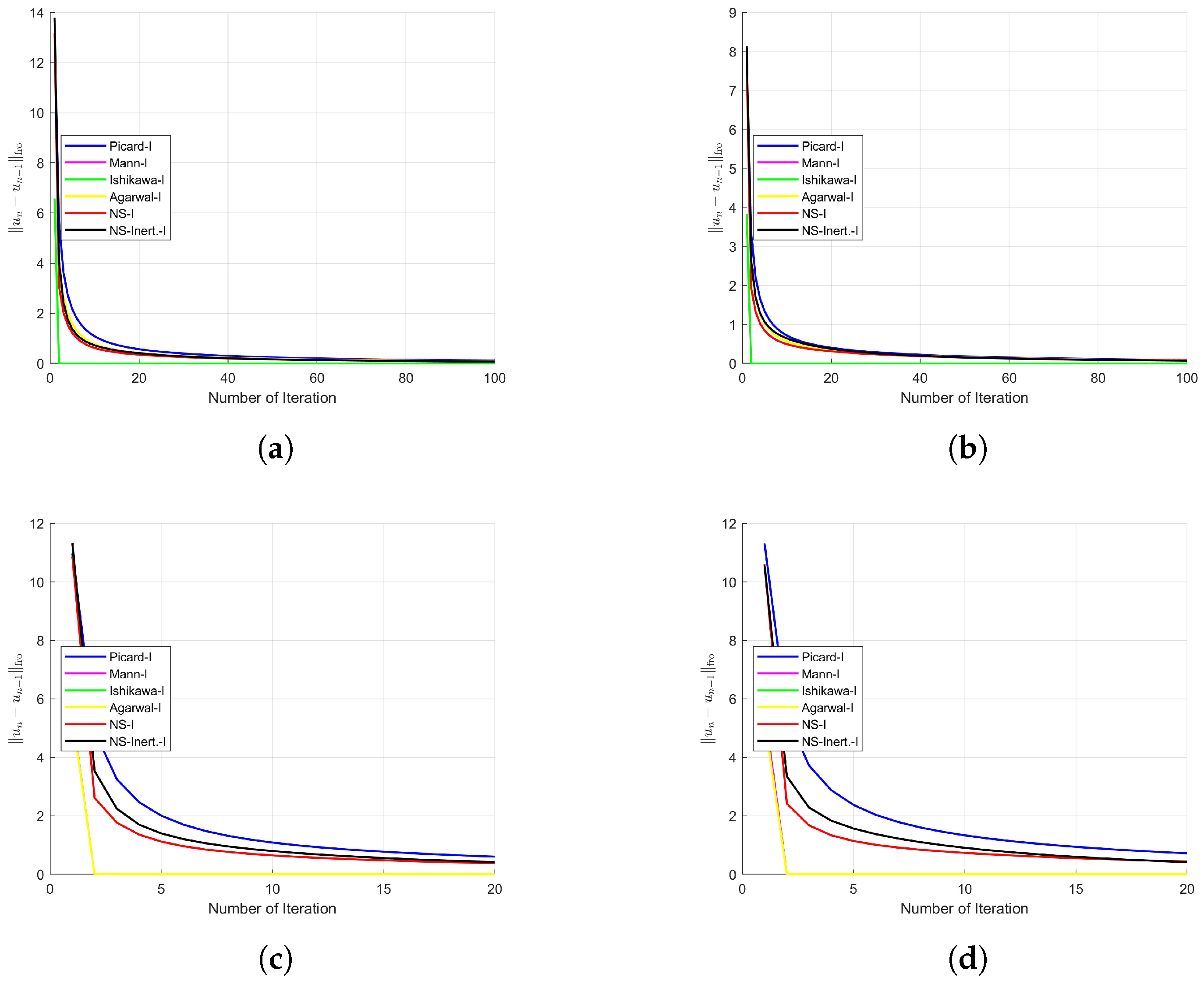
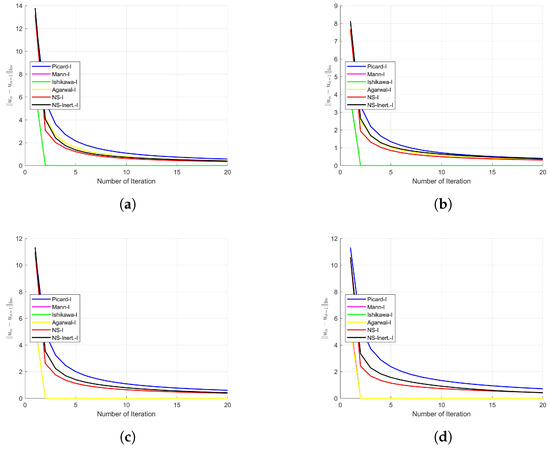
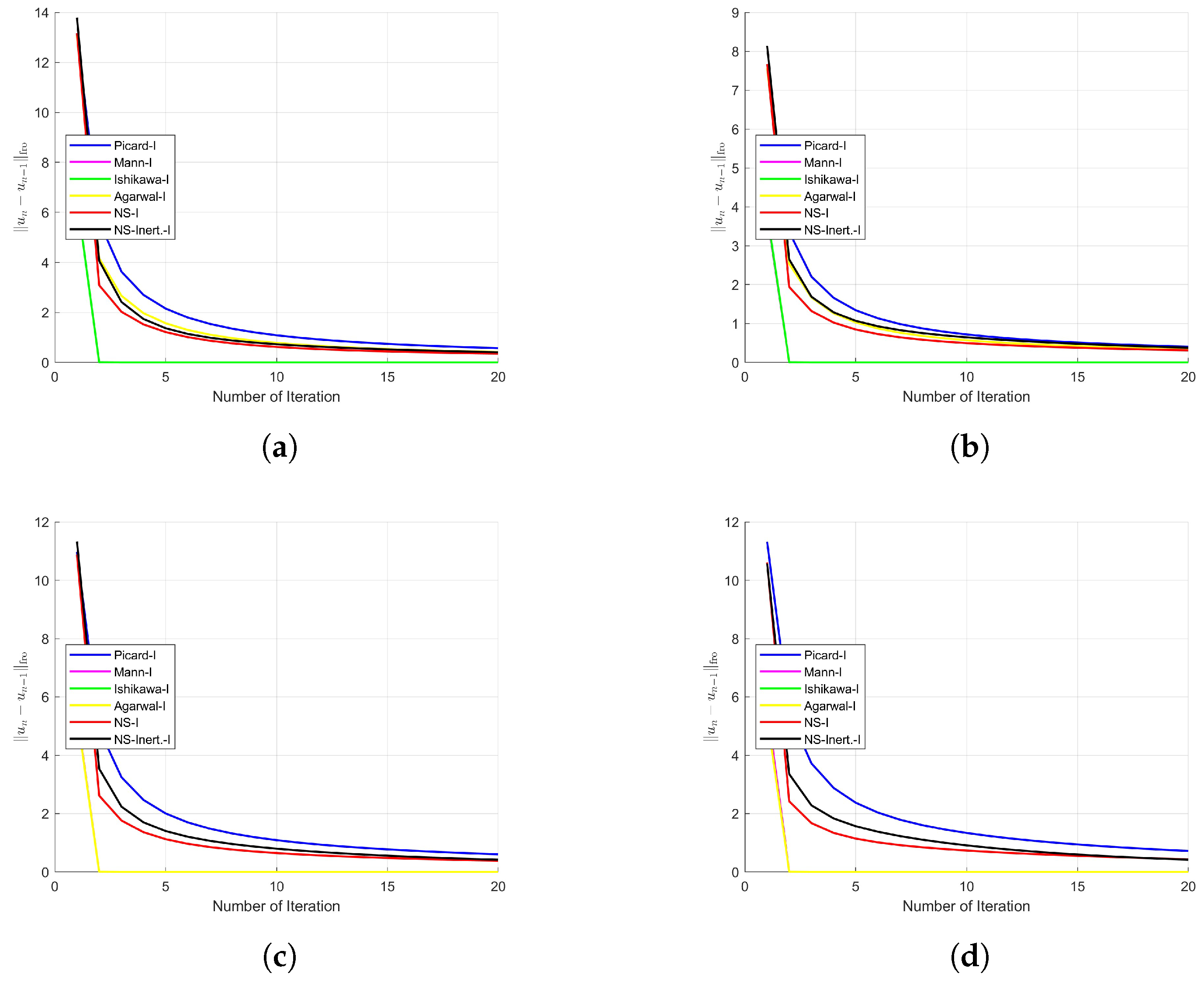
Figure 9 and Figure 10 indicate that the NS-Inert.-I algorithm demonstrates not only fast but also highly stable and consistent convergence. Notably, a significant divergence between algorithms is evident within the first 20 iterations.

Figure 9. Evolution of the Frobenius norm of successive iteration differences, $\parallel u_n-u_{n-1}{\parallel }_{\mathrm{fro}}$, during the first 100 iterations. (a) Airfield; (b) Harbour; (c) Kodim; (d) Clowns.

Figure 10. Evolution of the Frobenius norm of successive iteration differences, $\parallel u_n-u_{n-1}{\parallel }_{\mathrm{fro}}$, during the first 20 iterations. (a) Airfield; (b) Harbour; (c) Kodim; (d) Clowns.

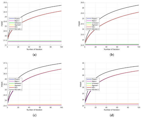
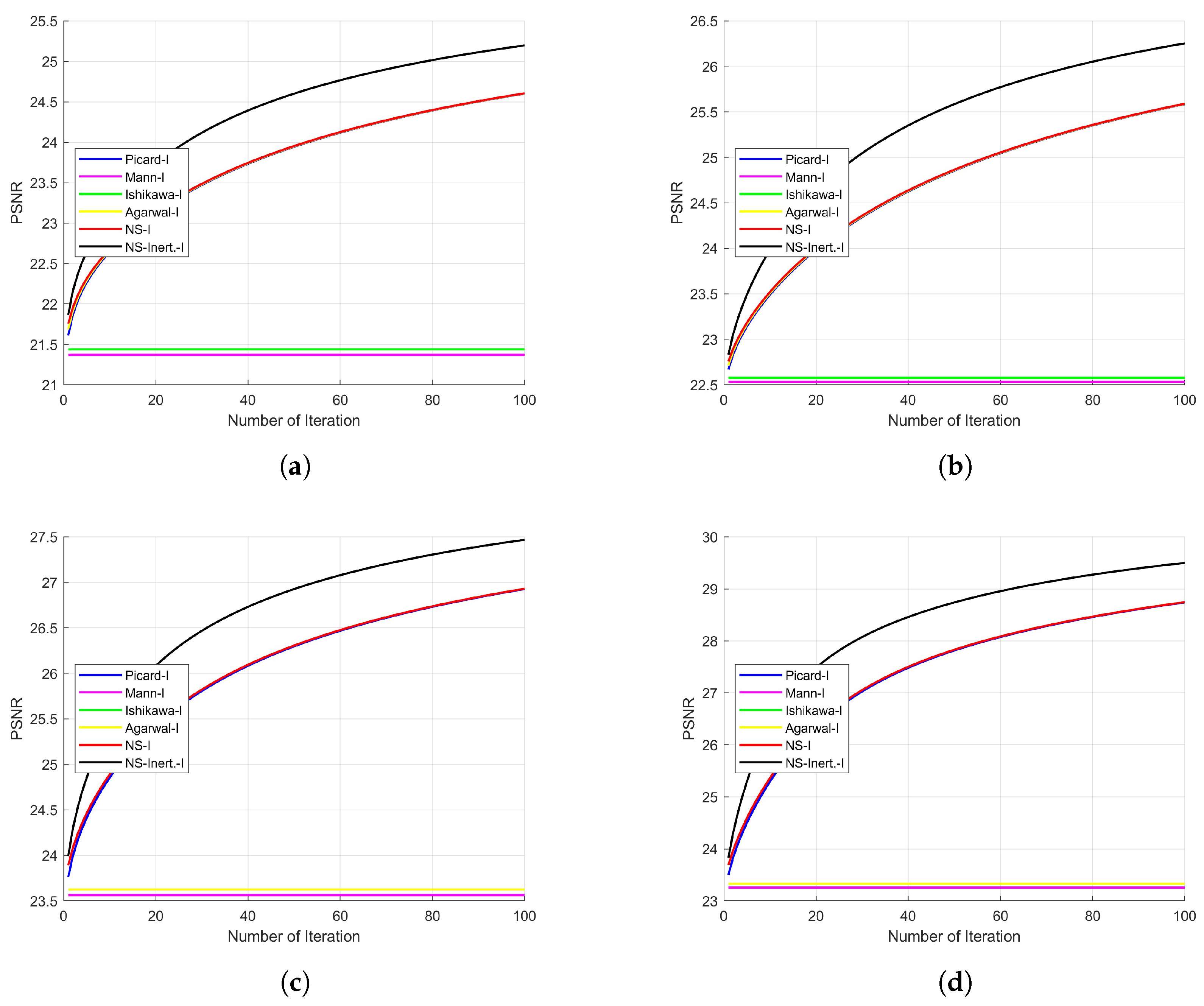
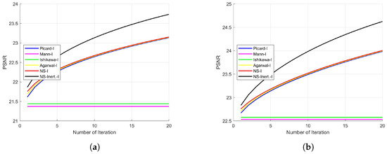
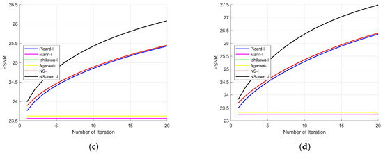
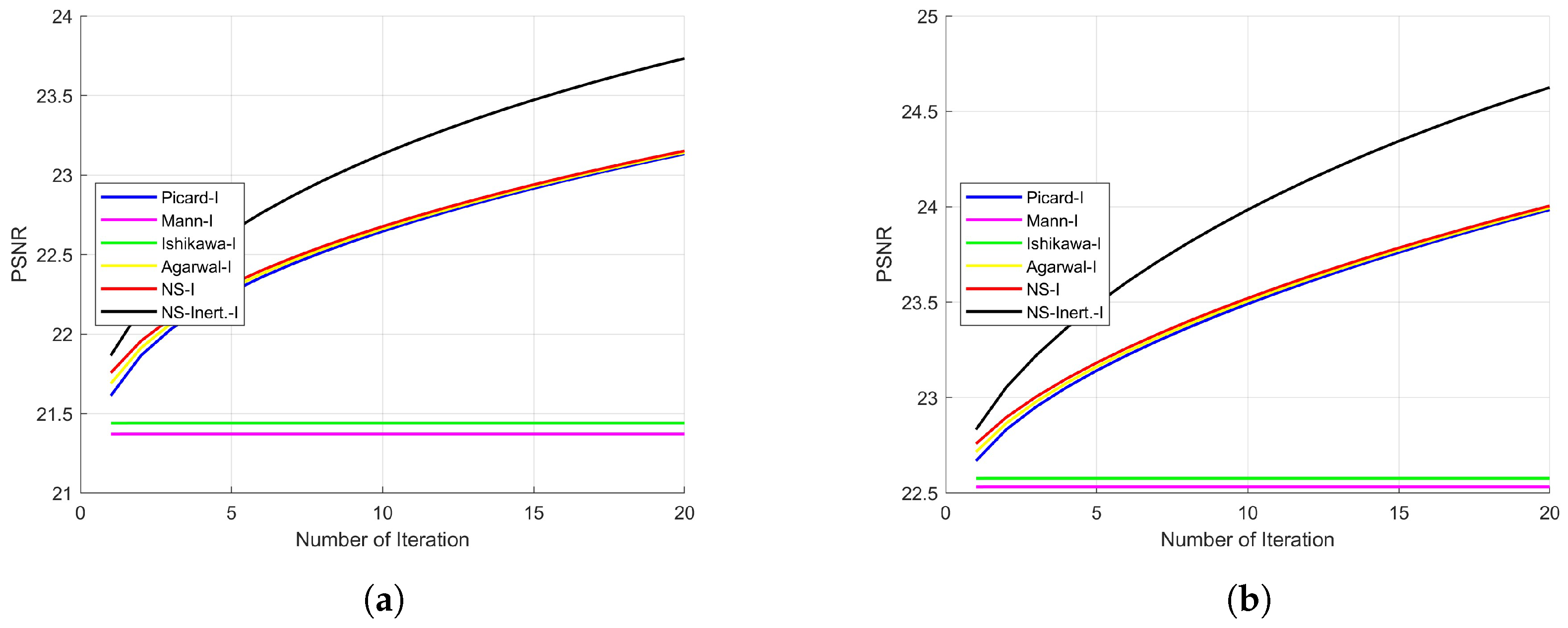
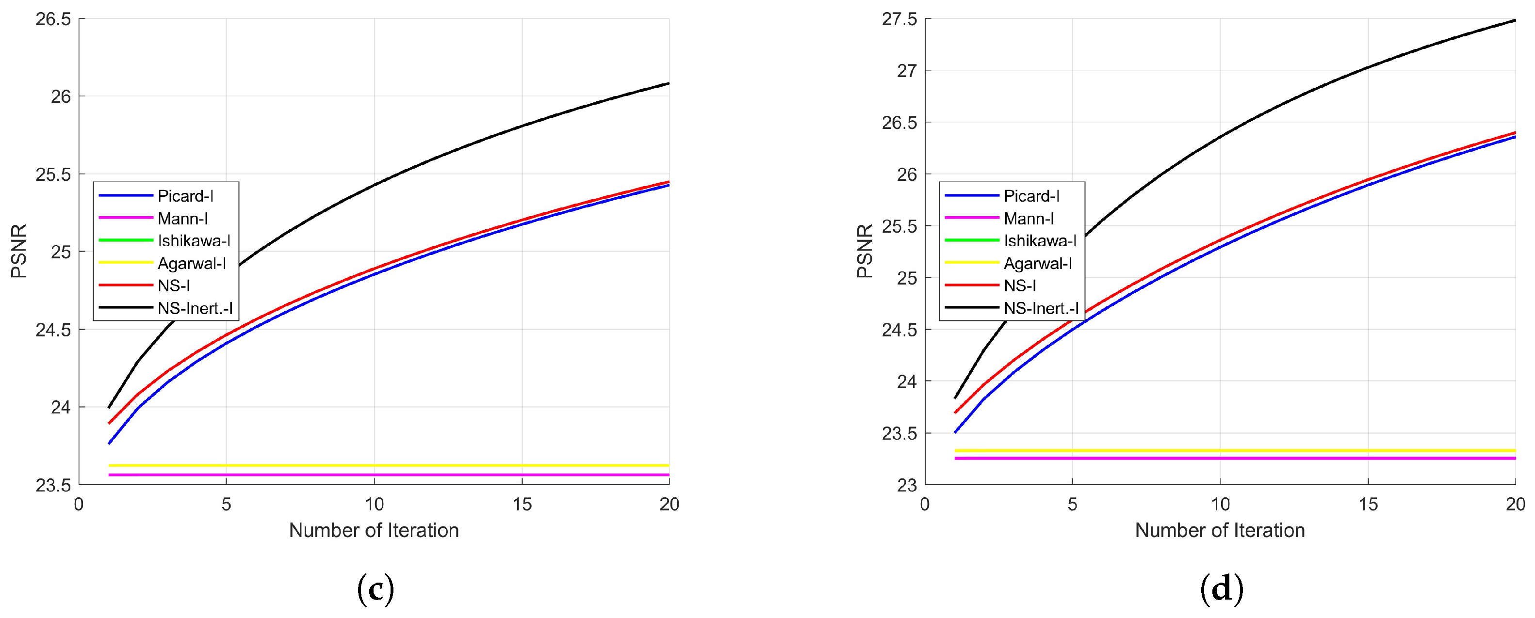
Figure 11 and Figure 12 illustrate that the NS-Inert.-I algorithm consistently attained the highest PSNR values throughout all iterations. Notably, it surpasses all other methods with respect to the final PSNR achieved at the end of the iteration algorithm. Taken together, both the visual and quantitative findings indicate that the T-operator-based NS-Inert.-I algorithms offer a pronounced and reliable advantage over classical ISTA and its variants, demonstrating rapid convergence in the early iterations as well as superior final image quality.

Figure 11. Evolution of PSNR values during the first 100 iterations. (a) Airfield; (b) Harbour; (c) Kodim; (d) Clowns.

Figure 12. Evolution of PSNR values during the first 20 iterations. (a) Airfield; (b) Harbour; (c) Kodim; (d) Clowns.

Figure 3, Figure 4, Figure 5 and Figure 6 provide a visual comparison of the restored images, while the quantitative performance of the algorithms is also assessed through the objective function values, the Frobenius norms of successive iteration differences, and the PSNR values reported in the subsequent figures and tables.

5. A Comparative Study of the Computational Performance of Various Algorithms via Fractal Generation

In fixed point theory, the emergence of fractal structures through iteration algorithms is closely related to the dynamic behavior of the underlying system and the complex geometry of the basins of attraction in the complex plane. During the iteration algorithm, different initial points may exhibit different dynamical behaviors: some points converge to a particular fixed point, some approach other roots, while others diverge toward infinity. Since each root is associated with its own basin of attraction, an initial point that lies within a particular basin will converge to the corresponding root under the selected iteration algorithm.

For example, if a polynomial has several distinct roots, the complex plane is naturally divided into different regions associated with these roots. These regions are known as basins of attraction. The boundaries separating these basins often have extremely complicated structures. When these boundaries are examined more closely, new geometric details continue to appear at different scales. Such behavior reveals a self-similar structure that repeats infinitely, which is one of the fundamental characteristics of fractal geometry. Consequently, the shapes generated by iteration algorithms frequently produce fractal patterns. Small variations in the initial points near the boundaries of attraction basins may cause the iterations to converge to completely different roots, which leads to chaotic behavior in those regions. The Mandelbrot and Julia sets are two of the most well-known and extensively studied examples of fractals generated by the iteration algorithm of a complex function. Benoit Mandelbrot [39] introduced the Mandelbrot set in the 1980s, while Pierre Fatou [40] and Gaston Julia independently created the Julia set in the early 20th century. The Julia set was initially introduced by [41]. Over time, mathematicians have developed several generalizations of these sets, including the use of different iteration algorithms derived from fixed point theory. These techniques have been utilized to generalize Julia and Mandelbrot sets [42,43,44,45,46,47].

Definition 3.

(Julia Set) Let $T_c:\mathbb{C}\to \mathbb{C}$ be a polynomial function that depends on $c\in \mathbb{C}$. The filled Julia set is

$$J_{T_c}=\{z\in \mathbb{C}:\parallel T_c^n\left(z\right)\parallel \nrightarrow \infty \mathit{as}n\to \infty \}$$

where $T_c^n\left(z\right)$ is the $n-th$ iteration of the function $T_c$. The Julia set $J{u}_{T_c}$ of the function $T_c$ is defined as the boundary of $J_{T_c}$, i.e., $J{u}_{T_c}=\partial J_{T_c}$.

Definition 4.

(Mandelbrot Set) Let $T_c:\mathbb{C}\to \mathbb{C}$ be a polynomial function that depends on $c\in \mathbb{C}$. The Maldelbrot set Mis the set of parameters c for which the Julia set filled, ie.,

$$M=\{c\in \mathbb{C}:J_{T_c}\mathit{is}\mathit{connected}.\}$$

Also, it is described as follows:

$$M=\{c\in \mathbb{C}:\parallel T_c^n\left(z^{*}\right)\parallel \nrightarrow \infty \mathit{as}n\to \infty \}$$

where $z^{*}$ is any critical point of $T_c$, i.e., $\partial T_c\left(z^{*}\right)=0$.

Definition 5.

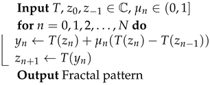
Let $T:\mathbb{C}\to \mathbb{C}$ be a complex mapping. The NS inertial-type orbit is defined as follows for an initial point $z_0,z_{-1}\in \mathbb{C}$:

Algorithm 4: NS inertial-type orbit

It is well known that $\left|\sin \left(z^n\right)\right|\le 1,\forall y,z\in \mathbb{C}$.

$$|\sin \left(z^n\right)|=\left|z^n-{\displaystyle \frac{z^{3n}}{3!}}+{\displaystyle \frac{z^{5n}}{5!}}-\dots \right|=\left|z^n\right|\left|1-{\displaystyle \frac{z^{2n}}{3!}}+{\displaystyle \frac{z^{4n}}{5!}}-\dots \right|$$

$$|\sin \left(y^n\right)|=\left|y^n-{\displaystyle \frac{y^{3n}}{3!}}+{\displaystyle \frac{y^{5n}}{5!}}-\dots \right|=\left|y^n\right|\left|1-{\displaystyle \frac{y^{2n}}{3!}}+{\displaystyle \frac{y^{4n}}{5!}}-\dots \right|$$

We take $T\left(z\right)$ as $T_c\left(z\right)$, with $y_0=y$, and $z_0=z$, and we assume that

$$\begin{array}{cc}\hfill \left(\mathrm{i}\right)& \left|1-{\displaystyle \frac{z^{2n}}{3!}}+{\displaystyle \frac{z^{4n}}{5!}}-\dots \right|\ge \left|{\tau }_1\right|,\hfill \\ \hfill \left(\mathrm{ii}\right)& \left|1-{\displaystyle \frac{y^{2n}}{3!}}+{\displaystyle \frac{y^{4n}}{5!}}-\dots \right|\ge \left|{\tau }_2\right|,\hfill \end{array}$$

where $|{\tau }_1|,|{\tau }_2|\in (0,1]$, except for the values of $y,z$ for which

$$|{\tau }_1|=|{\tau }_2|=0.$$

By utilizing four distinct celebrated iterations, we prove here an escape criterion for the transcendental complex sine function of the type

$$T\left(z\right)=\sin \left(z^n\right)+az+c,a,c\in \mathbb{C},n\ge 2.$$

Theorem 6.

Let $T_c\left(z\right)=\sin \left(z^n\right)+az+c$, $a,c\in \mathbb{C},n\ge 2$, $\left|z\right|\ge \left|c\right|>{\left({\displaystyle \frac{2(1+|a\left|\right)}{|{\tau }_1|}}\right)}^{{\displaystyle \frac{1}{n-1}}}$, and $\left|z\right|\ge \left|c\right|>{\left({\displaystyle \frac{2(1+|a\left|\right)}{|{\tau }_2|}}\right)}^{{\displaystyle \frac{1}{n-1}}}$. Let the sequence ${\left\{z_k\right\}}_{k\in \mathbb{N}}$ be generated by Algorithm 4, that is,

$$z_{k+1}=T\left(y_k\right),y_k=T\left(z_k\right)+\mu \left(T\left(z_k\right)-T\left(z_{k-1}\right)\right),k\ge 1,$$

where $\mu \in [0,1]$.

Assume that, for all $z\in \mathbb{C}$,

$$|\sin \left(z^n\right)|\ge |{\tau }_1{\left|\right|z|}^n,|\sin \left(y^n\right)|\ge |{\tau }_2{\left|\right|y|}^n,$$

where $|{\tau }_1|,|{\tau }_2|\in (0,1]$, for all k, and that for some $\rho \ge 0$,

$$|T\left(z_{k-1}\right)|\le \rho |T\left(z_k\right)|,0\le \rho <1+{\displaystyle \frac{1}{{\mu }_k}},\forall k\ge 0.$$

Define

$${\delta }_k:=1+{\mu }_k-{\mu }_k\rho >0.$$

Then, $|z_k|\to \infty$ as $k\to \infty$.

Proof. 

Let $T\left(z\right)=\sin \left(z^n\right)+az+c$, $z_0=z$ and using the Algorithm 4, we have

$$|y_k|=|T\left(z_k\right)+\mu (T\left(z_k\right)-T\left(z_{k-1}\right))|.$$

If $k=0$,

$$\begin{array}{cc}\hfill |y_0|& =|T\left(z_0\right)+\mu (T\left(z_0\right)-T\left(z_{-1}\right))|\hfill \\ \hfill & =|(1+\mu )T\left(z_0\right)-\mu \left(T\left(z_{-1}\right)\right)|\hfill \\ \hfill & \ge (1+\mu )|T\left(z_0\right)|-\mu |\left(T\left(z_{-1}\right)\right)|,|T\left(z_{k-1}\right)|\le \rho |T\left(z_k\right)|,0\le \rho <1+{\displaystyle \frac{1}{{\mu }_k}},\forall k\ge 0\hfill \\ \hfill & \ge (1+\mu -\mu \rho )\left|T\right(z\left)\right|\hfill \\ \hfill & =\delta \left|T\right(z\left)\right|\hfill \\ \hfill & =\delta \left|\sin \right(z^n)+az+c|\hfill \\ \hfill & \ge \delta |\sin \left(z^n\right)|-\delta |az|-\delta |c|,|\sin \left(z^n\right)|\ge |{\tau }_1{\left|\right|z|}^n\hfill \\ \hfill & \ge \delta |{\tau }_1\left|\right|z^n|-\delta |a\left|\right|z|-\delta |z|,|z|\ge \left|c\right|,\hfill \\ \hfill & \ge \delta \left(\right|{\tau }_1\left|\right|z^n|-|z\left|\right(1+\left|a\right|\left)\right),\mu \in (0,1],\hfill \\ \hfill & =\left|z\right|\delta (1+\left|a\right|)\left({\displaystyle \frac{{\tau }_1\left|\right|z^{n-1}|}{1+\left|a\right|}}-1\right).\hfill \end{array}$$

(34)

Since

$$|\sin \left(z^n\right)|=\left|z^n-{\displaystyle \frac{z^{3n}}{3!}}+{\displaystyle \frac{z^{5n}}{5!}}-\dots \right|\ge |{\tau }_1\left|\right|z^n|,$$

where $z\in \mathbb{C}$, except the values of z for which $|{\tau }_1|=0$, $|{\tau }_1|\in (0,1]$, we get

$$\left|y\right|\ge {\displaystyle \frac{\left|y\right|}{\delta (1+|a\left|\right)}}=\left|z\right|\left({\displaystyle \frac{|{\tau }_1\left|\right|z^{n-1}|}{1+\left|a\right|}}-1\right).$$

Since

$$\left|z\right|>{\left({\displaystyle \frac{2(1+|a\left|\right)}{|{\tau }_1|}}\right)}^{{\displaystyle \frac{1}{n-1}}},$$

this provides that

$$|y^n{|>|z|}^n{\left({\displaystyle \frac{|{\tau }_1\left|\right|z^{n-1}|}{1+\left|a\right|}}-1\right)}^n\ge |{\tau }_1{\left|\right|z|}^n.$$

Now, for the next step of NS inertial-type iteration algorithm, we have

$$|z_{k+1}|=|T\left(y_k\right)|.$$

Again, if $k=0$,

$$\begin{array}{cc}\hfill |z_1|& =\left|T\right(y\left)\right|\hfill \\ \hfill & =\left|\right(\sin \left(y^n\right)+ay+c\left)\right|\hfill \\ \hfill & \ge \left|\sin \right(y^n\left)\right|-ay|-|c|-\hfill \\ \hfill & \ge \left|\sin \right(y^n\left)\right|-\left|a\right|\left|y\right|-\left|z\right|,\left|z\right|\ge \left|c\right|,\hfill \\ \hfill & \ge |{\tau }_2\left|\right|y^n|-|y\left|\right|a|-|z|\hfill \\ \hfill & \ge |{\tau }_1\left|\right|{\tau }_2\left|\right|z^n|-|{\tau }_1\left|\right|z\left|\right|a|-\left|z\right|\hfill \\ \hfill & =|{\tau }_1\left|\right|{\tau }_2\left|\right|z^n|-|z\left|\right|a|-|z|,{\tau }_1\in (0,1],\hfill \\ \hfill & =|{\tau }_1\left|\right|{\tau }_2\left|\right|z^n|-|z\left|\right(1+\left|a\right|)\hfill \\ \hfill & =\left|z\right|(1+\left|a\right|)\left({\displaystyle \frac{|{\tau }_1\left|\right|{\tau }_2\left|\right|z^{n-1}|}{1+\left|a\right|}}-1\right).\hfill \end{array}$$

This is because

$$|\sin \left(y^n\right)|=\left|y^n-{\displaystyle \frac{y^{3n}}{3!}}+{\displaystyle \frac{y^{5n}}{5!}}-\dots \right|\ge |{\tau }_2\left|\right|y^n|,$$

where $z\in \mathbb{C}$, except the values of z for which $|{\tau }_2|=0$, $|{\tau }_2|\in (0,1]$. In addition, $\left|y\right|\ge \beta |{\tau }_1\left|\right|z|$. Thus, we get

$$|z_1|\ge {\displaystyle \frac{|z_1|}{1+\left|a\right|}}=\left|z\right|\left({\displaystyle \frac{|{\tau }_1\left|\right|{\tau }_2\left|\right|z^{n-1}|}{1+\left|a\right|}}-1\right).$$

Now, on iterating up to kth term, we obtain

$$|z_2|\ge |z|{\left({\displaystyle \frac{|{\tau }_1\left|\right|{\tau }_2\left|\right|z^{n-1}|}{1+\left|a\right|}}-1\right)}^2$$

$$|z_3|\ge |z|{\left({\displaystyle \frac{|{\tau }_1\left|\right|{\tau }_2\left|\right|z^{n-1}|}{1+\left|a\right|}}-1\right)}^3$$

$$|z_4|\ge |z|{\left({\displaystyle \frac{|{\tau }_1\left|\right|{\tau }_2\left|\right|z^{n-1}|}{1+\left|a\right|}}-1\right)}^4$$

$$⋮$$

$$|z_k|\ge |z|{\left({\displaystyle \frac{|{\tau }_1\left|\right|{\tau }_2\left|\right|z^{n-1}|}{1+\left|a\right|}}-1\right)}^k.$$

Since $\left|z\right|\ge \left|c\right|>{\left({\displaystyle \frac{2(1+|a\left|\right)}{|{\tau }_1|}}\right)}^{{\displaystyle \frac{1}{n-1}}}$ and $\left|z\right|\ge \left|c\right|>{\left({\displaystyle \frac{2(1+|a\left|\right)}{|{\tau }_2|}}\right)}^{{\displaystyle \frac{1}{n-1}}}$, $|{\tau }_1|,|{\tau }_2|\in (0,1)$, this implies that

$$\left|z\right|\ge \left|c\right|>{\left({\displaystyle \frac{2(1+|a\left|\right)}{|{\tau }_1\left|\right|{\tau }_2|}}\right)}^{{\displaystyle \frac{1}{n-1}}}.$$

Hence,

$${\displaystyle \frac{|{\tau }_1\left|\right|{\tau }_2\left|\right|z^{n-1}|}{(1+|a\left|\right)}}-1>1$$

and the orbit of z tends to infinity, that is, $|z_k|\to \infty$ when $k\to \infty$.    □

Corollary 1.

Let $|z_m|>\max \left\{\left|c\right|,{\left({\displaystyle \frac{2(1+|a\left|\right)}{|{\tau }_1|}}\right)}^{{\displaystyle \frac{1}{n-1}}},{\left({\displaystyle \frac{2(1+|a\left|\right)}{|{\tau }_1\left|\right|{\tau }_2|}}\right)}^{{\displaystyle \frac{1}{n-1}}}\right\},m\ge 0.$

Since

$${\displaystyle \frac{|{\tau }_1\left|\right|{\tau }_2\left|\right|z^{n-1}|}{(1+|a\left|\right)}}-1>1,$$

therefore,

$$|z_{m+k}|>|z|{\left({\displaystyle \frac{|{\tau }_1\left|\right|{\tau }_2\left|\right|z^{n-1}|}{(1+|a\left|\right)}}\right)}^{m+k}.$$

Hence, $|z_k|\to \infty$ when $k\to \infty$.

Remark 3.

For the transcendental complex function

$$T_c\left(z\right)=\sin \left(z^n\right)+az+c,a,c\in \mathbb{C},n\ge 2,$$

the escape criteria established via different fixed point iterations (Picard, Mann, Ishikawa and Noor) ensure that the generated orbit diverges to infinity under suitable initial conditions.

More precisely, as proved in [48], the following hold:

1. 

Under the Picard iteration algorithm, if 

$$\left|z\right|\ge \left|c\right|>{\left({\displaystyle \frac{2(1+|a\left|\right)}{|{\tau }_1|}}\right)}^{{\displaystyle \frac{1}{n-1}}},$$

then $|z_k|\to \infty$.

2. 

Under the Mann iteration algorithm, if 

$$\left|z\right|\ge \left|c\right|>{\left({\displaystyle \frac{2(1+|a\left|\right)}{\alpha |{\tau }_1|}}\right)}^{{\displaystyle \frac{1}{n-1}}},$$

then $|z_k|\to \infty$.

3. 

Under the Ishikawa iteration algorithm, if

$$\left|z\right|\ge \left|c\right|>{\left({\displaystyle \frac{2(1+|a\left|\right)}{\alpha |{\tau }_1|}}\right)}^{{\displaystyle \frac{1}{n-1}}}\mathit{and}\left|z\right|\ge \left|c\right|>{\left({\displaystyle \frac{2(1+|a\left|\right)}{\beta |{\tau }_2|}}\right)}^{{\displaystyle \frac{1}{n-1}}},$$

then $|z_k|\to \infty$.

4. 

Under the Noor iteration algorithm, if 

$$\left|z\right|\ge \left|c\right|>{\left({\displaystyle \frac{2(1+|a\left|\right)}{\alpha |{\tau }_1|}}\right)}^{{\displaystyle \frac{1}{n-1}}},\left|z\right|\ge \left|c\right|>{\left({\displaystyle \frac{2(1+|a\left|\right)}{\beta |{\tau }_2|}}\right)}^{{\displaystyle \frac{1}{n-1}}},$$

$$\mathit{and}\left|z\right|\ge \left|c\right|>{\left({\displaystyle \frac{2(1+|a\left|\right)}{\gamma |{\tau }_3|}}\right)}^{{\displaystyle \frac{1}{n-1}}},$$

then $|z_k|\to \infty$.

These results provide unified escape criteria ensuring divergence of the orbit, which play a fundamental role in the generation of Julia sets for the function $T_c$.

Corollary 2.

Let $T_c\left(z\right)=\sin \left(z^n\right)+az+c$, $a,c\in \mathbb{C},n\ge 2$. Consider the Normal Siteration algorithm obtained from the Ishikawa iteration algorithm by taking $\alpha =1$.

If the initial point $z\in \mathbb{C}$ satisfies

$$\left|z\right|\ge \left|c\right|>{\left({\displaystyle \frac{2(1+|a\left|\right)}{|{\tau }_1|}}\right)}^{{\displaystyle \frac{1}{n-1}}}\mathit{and}\left|z\right|\ge \left|c\right|>{\left({\displaystyle \frac{2(1+|a\left|\right)}{\beta |{\tau }_2|}}\right)}^{{\displaystyle \frac{1}{n-1}}},$$

then the orbit $\left\{z_k\right\}$ generated by the Normal S iteration algorithm diverges to infinity, that is,

$$|z_k|\to \infty \mathit{as}k\to \infty .$$

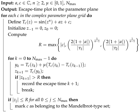
Algorithm 5: Mandelbrot-type set generation via NS inertial-type iteration algorithm

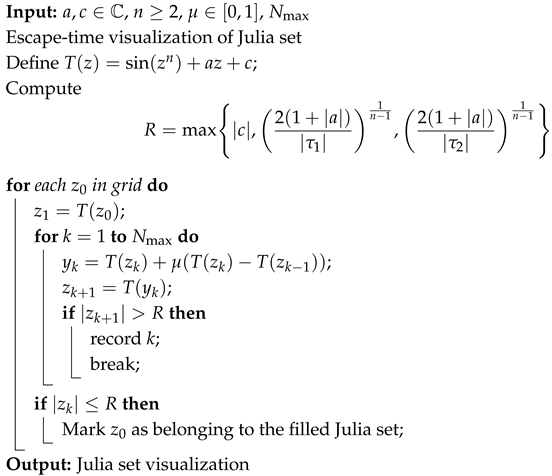
Algorithm 6: Julia set generation via NS inertial-type iteration algorithm

Because iterative dynamical systems often exhibit chaotic boundary behavior when multiple attracting fixed points exist, they naturally provide a mathematical foundation for the formation of fractal structures. As a result, iteration algorithms produce fractal patterns in the complex plane, since the boundaries separating regions that converge to different fixed points typically display chaotic and self-similar structures.

In theoretical studies, iteration algorithms are generally compared in terms of convergence rates or error analyses. However, fractal visualizations provide an effective way to observe the overall dynamical behavior of these algorithms. Different iteration algorithms may generate different basins of attraction, distinct chaotic boundaries, and varying convergence rates. Therefore, comparing fixed point iteration algorithms through fractal patterns is particularly valuable both for numerical analysis and complex dynamics. Such visualizations allow researchers to understand the convergence behavior of iteration algorithm in an intuitive and geometric way. In fractal representations, the convergence speed toward roots and the number of iterations required are usually expressed through color variations. In this way, it becomes possible to visually identify which fixed point iteration algorithm converges more rapidly to a root and which algorithm demonstrates a more stable convergence behavior in the complex plane.

The fixed point iteration algorithm considered in this study include the Picard, Mann, Ishikawa, Agarwal, Normal S, and NS inertial-type iteration algorithms. The fractal visualizations obtained through these iteration algorithms reveal that the NS inertial-type iteration algorithm exhibits a more stable and dynamically efficient behavior compared with the other fixed point iteration algorithms. In particular, the fractal patterns generated by this algorithm indicate stronger convergence characteristics and a more consistent dynamical structure in the complex plane.

Furthermore, motivated by recent studies in the literature, this work also aims to obtain Julia set and Mandelbrot-type fractal visualizations based on the escape criteria for the function $T(z,n)=\sin \left(z^n\right)+az+c$ were generated using the NS inertial-type iteration algorithms described in Algorithms 5 and 6. The resulting fractal images demonstrate that the NS inertial-type iteration algorithm provides a more effective and practical framework compared with the other iteration algorithms considered in this study. The fractal visualizations of the complex function

$$T(z,n)=\sin \left(z^n\right)+az+c$$

are generated using the Picard, Mann, Ishikawa, Agarwal, Normal S, and NS inertial-type iteration algorithms for different parameter values. The computations are performed in the complex plane within the domain $[-3,3]\times [-2,2]$ using the escape time algorithm with an image resolution of 1200 pixels in the x direction and 800 pixels in the y direction. For the escape radius

$$R_1={\left({\displaystyle \frac{2(1+|a\left|\right)}{|{\tau }_1|}}\right)}^{{\displaystyle \frac{1}{n-1}}},R_2={\left({\displaystyle \frac{2(1+|a\left|\right)}{|{\tau }_1\left|\right|{\tau }_2|}}\right)}^{{\displaystyle \frac{1}{n-1}}},$$

$$R=\max \left(\left|c\right|,R_1,R_2\right).$$

a maximum of 500 iterations is applied. Also, the resulting fractal structures are visualized using the colorcube colormap.

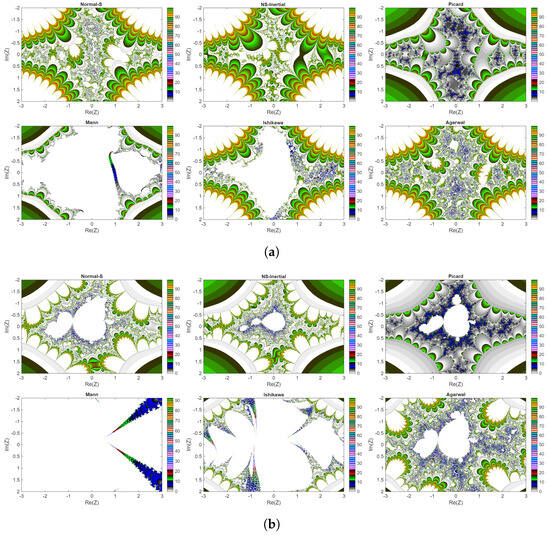
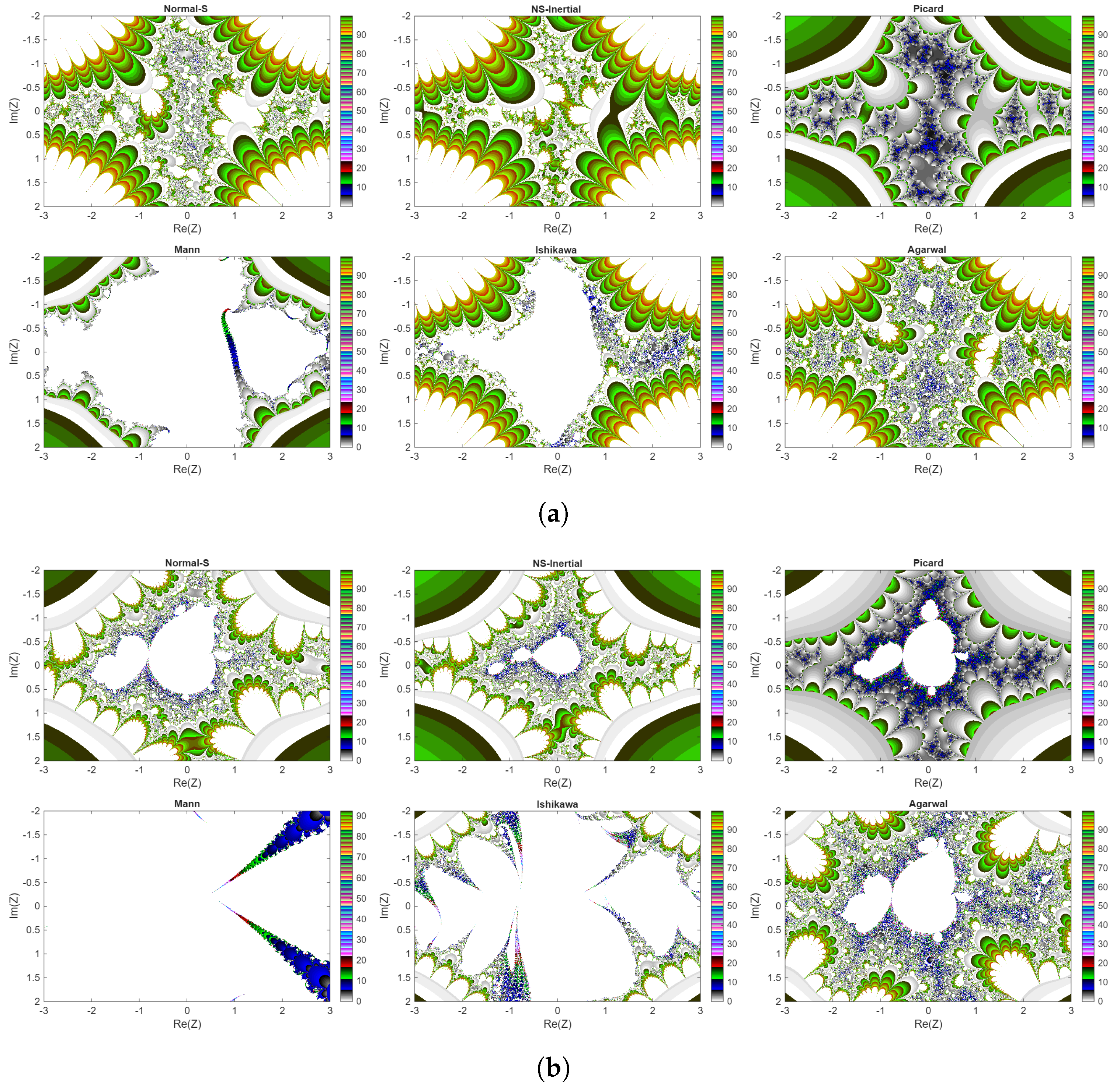
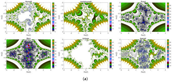
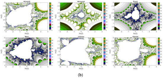
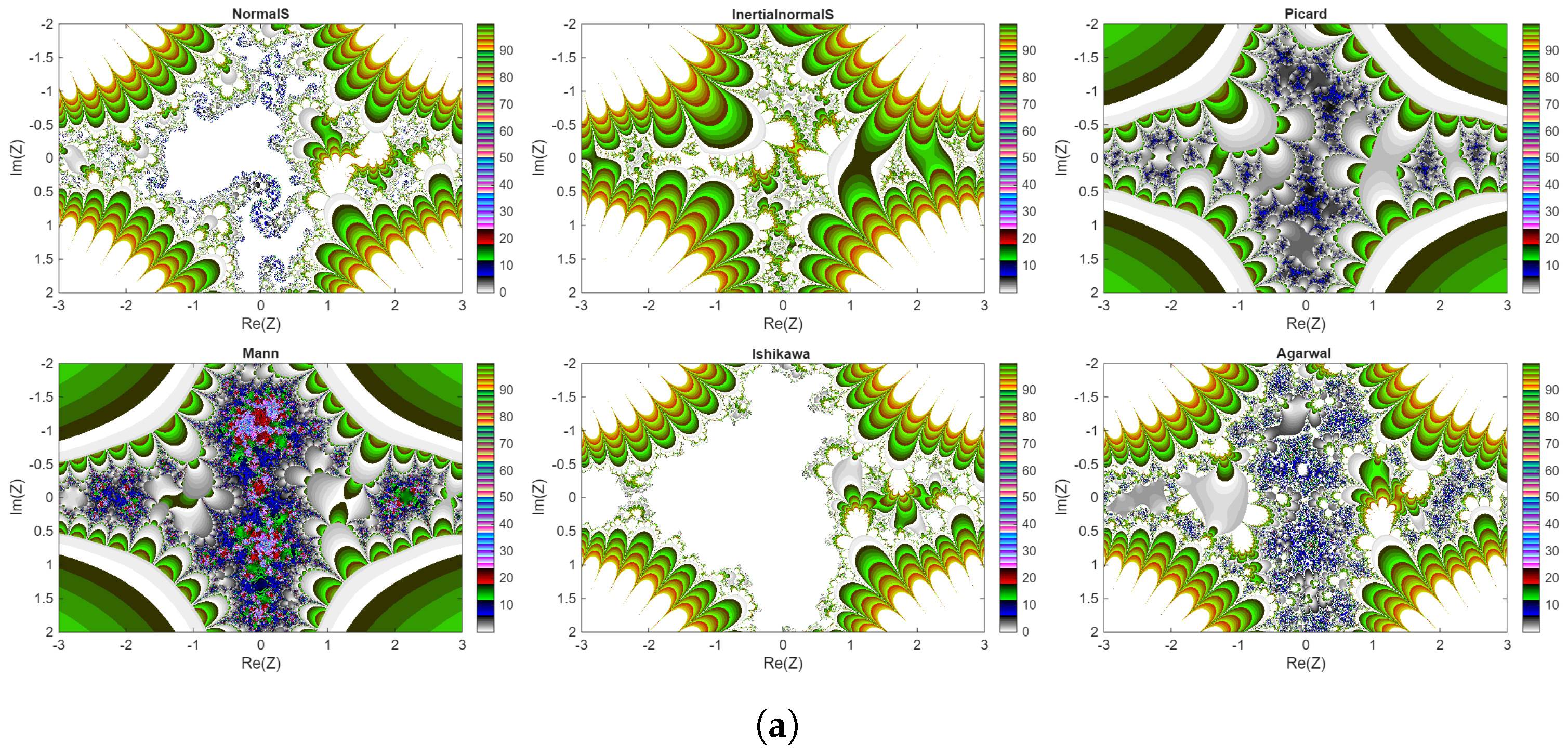
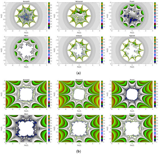
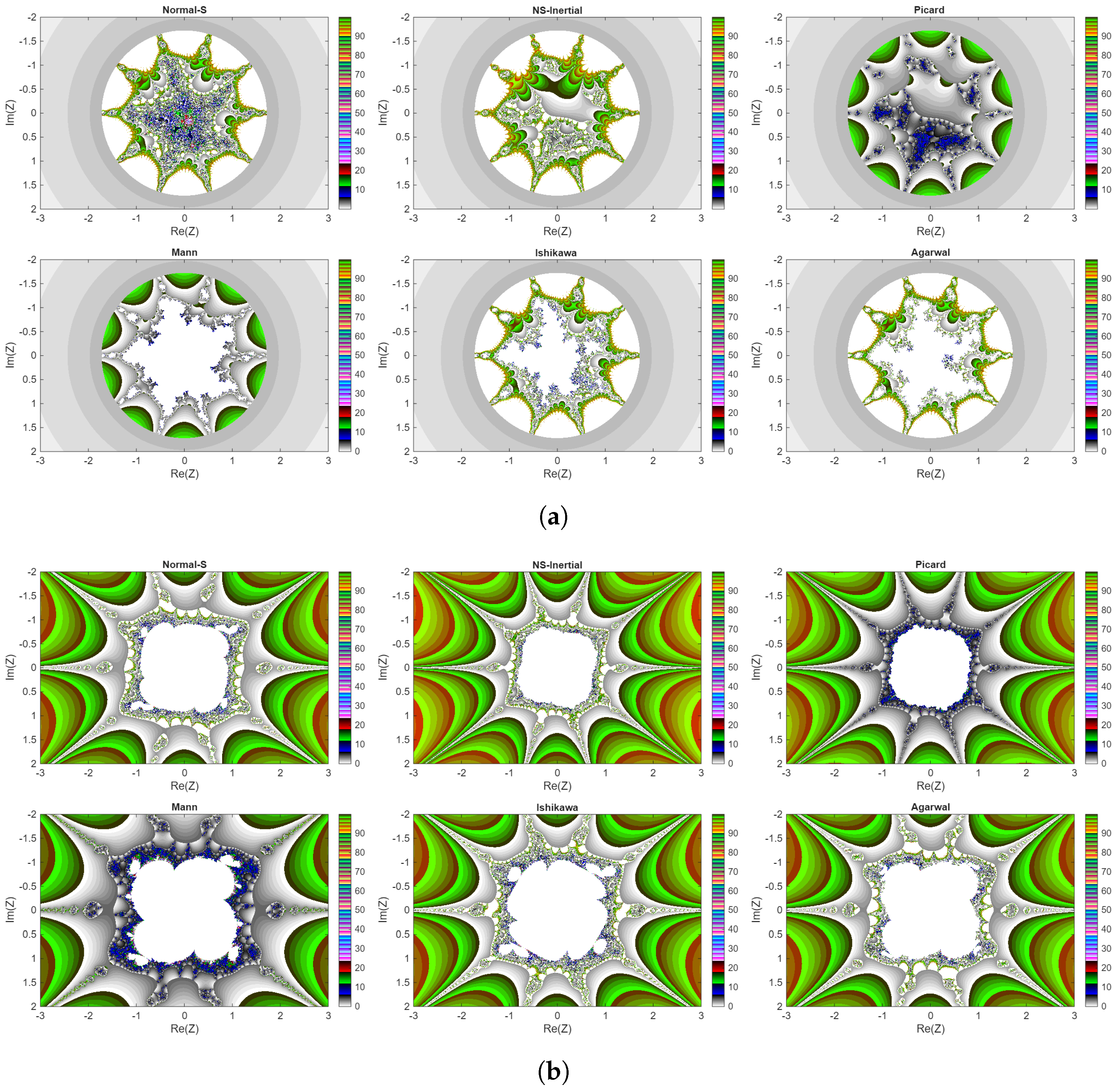
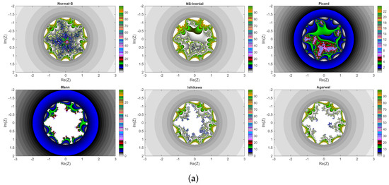
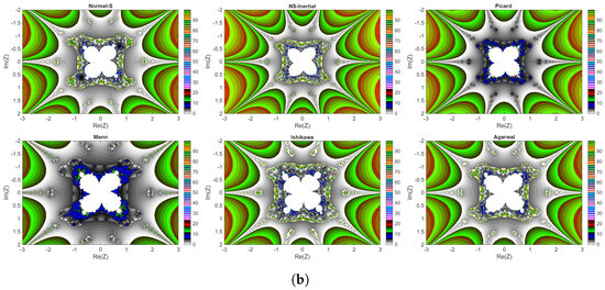
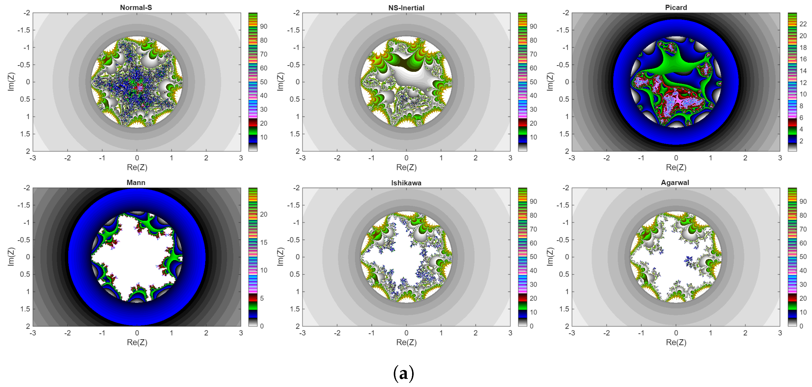
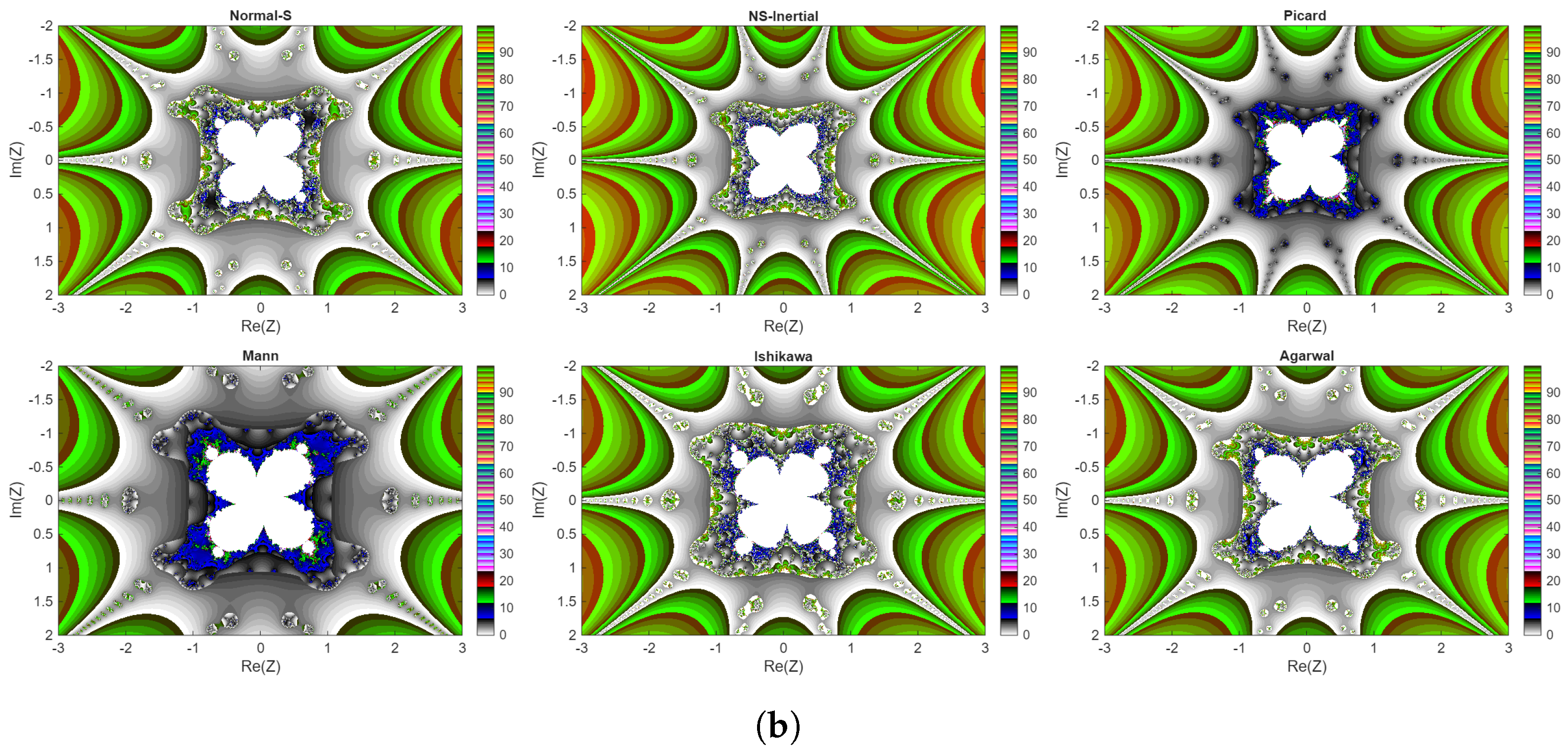
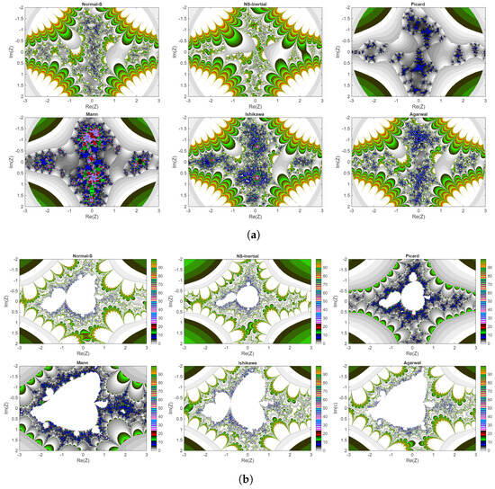
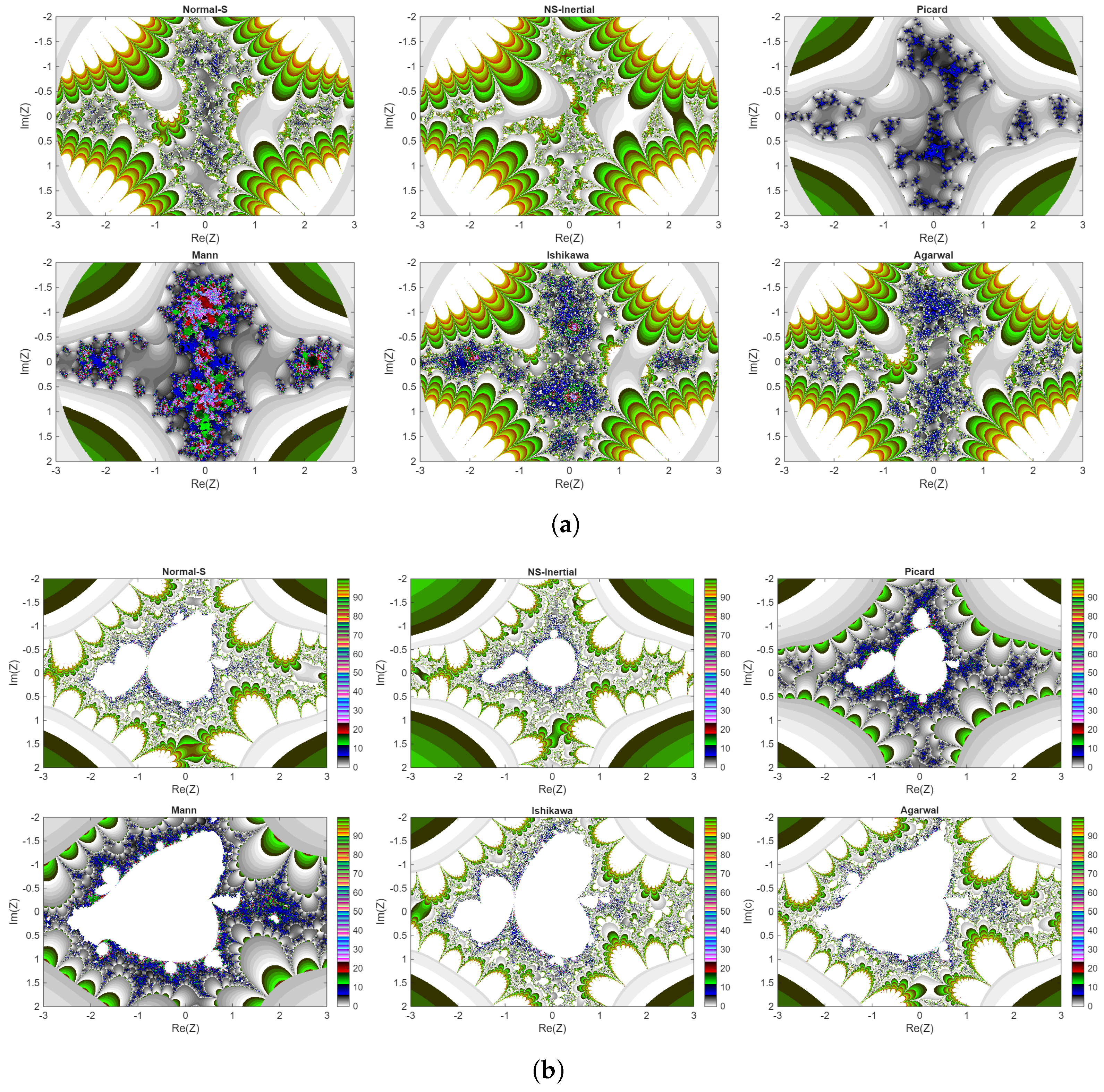
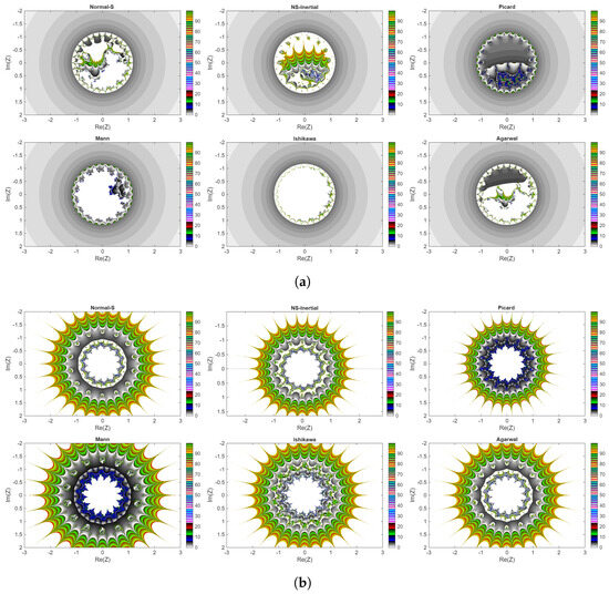
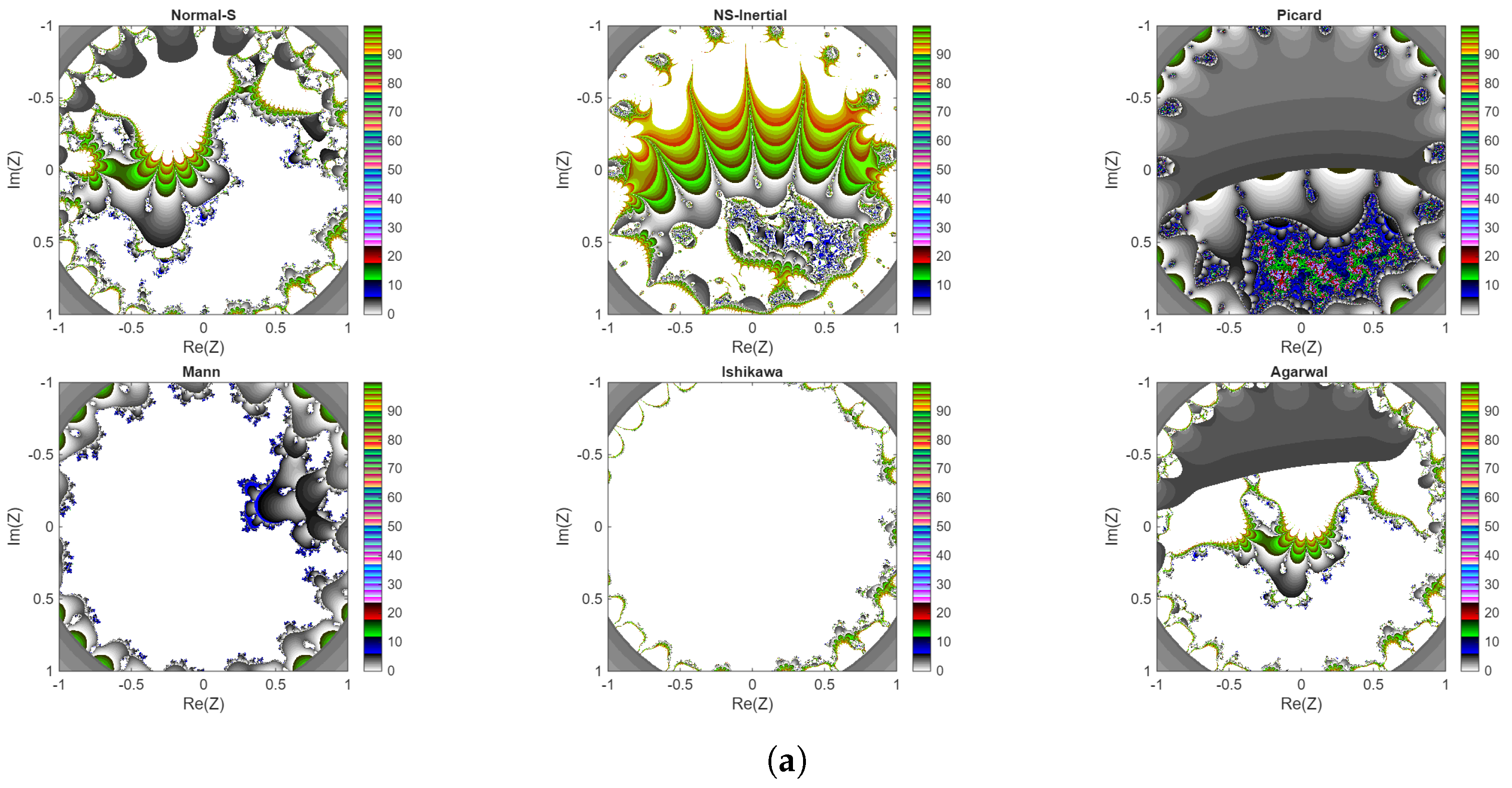
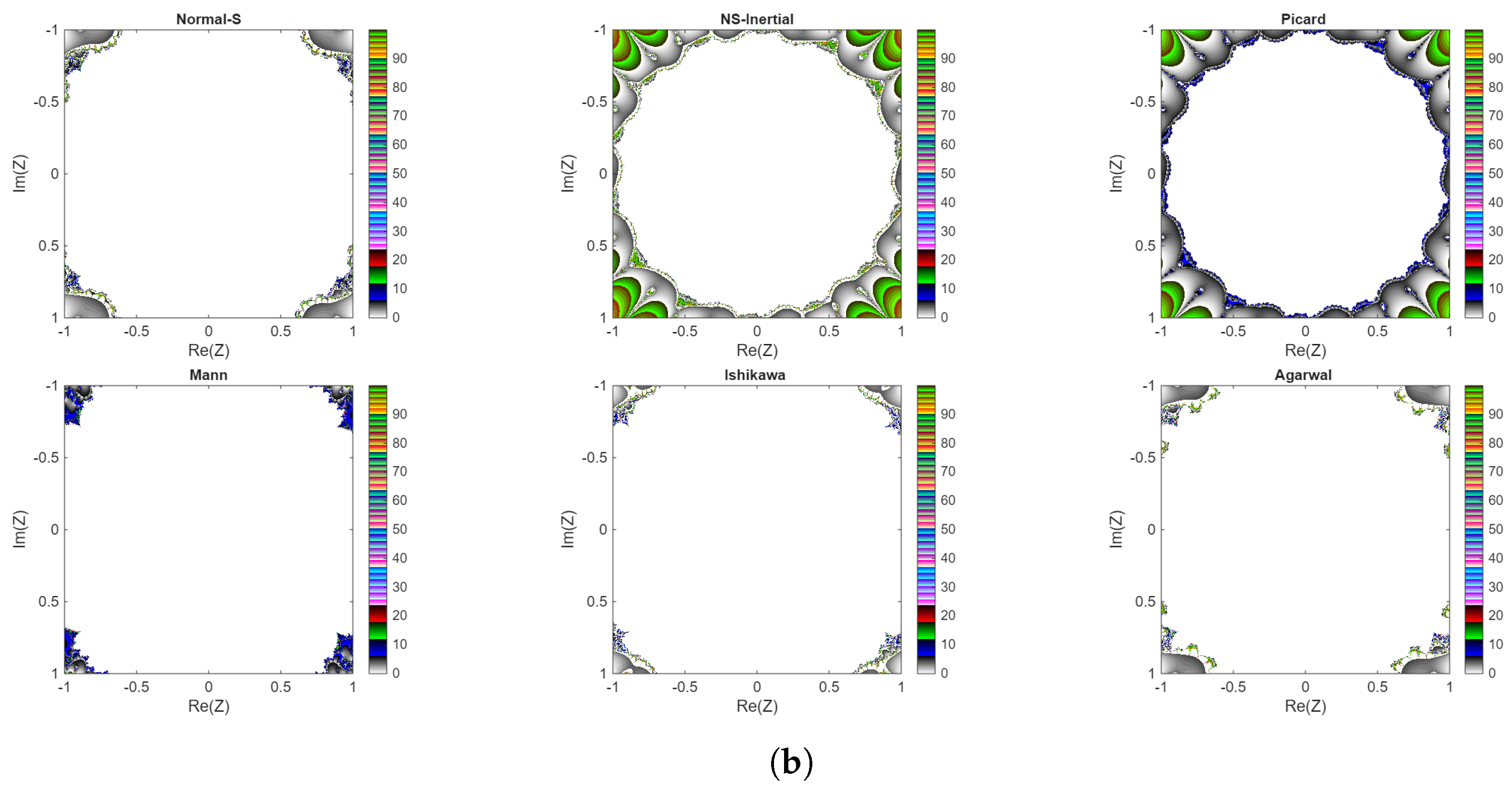
In Figure 13, the Julia set and Mandelbrot-type fractals are generated using the parameter values $c=-0.158+0.86i$, $a=-0.4+0.3i$, $\tau =0.8$, $u_1=0.40$, $\alpha =0.70$, $\beta =0.80$, and $n=2$. For the NS inertial-type iteration algorithm, the inertia parameter is chosen as $\mu =0.30$. The resulting fractal images reveal interesting geometric patterns, demonstrating that different fixed point iteration algorithms applied to the same nonlinear complex function can produce significantly different fractal structures.

Figure 13. Fractal structures generated from the complex function $T\left(z\right)=\sin \left(z^n\right)+az+c$ using different fixed point iteration algorithms in the complex plane for the parameters $\alpha =0.70$, $\beta =0.80$, $\mu =0.30$, and $n=2$. (a) Julia set; (b) Mandelbrot.

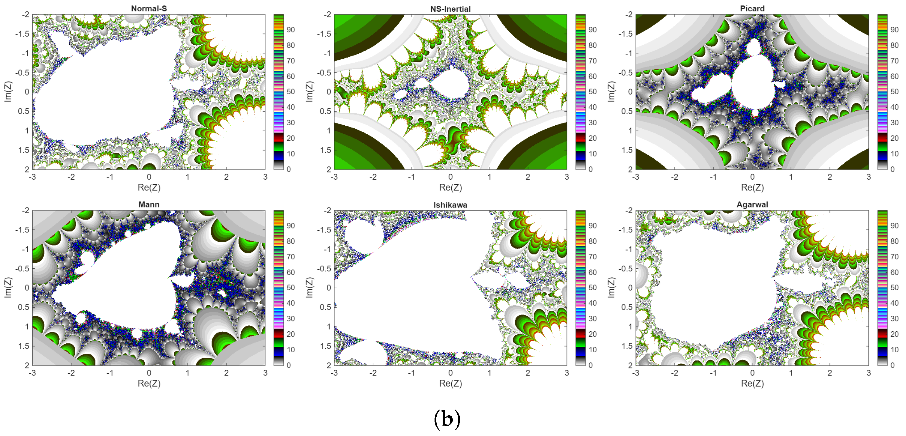
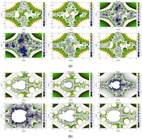
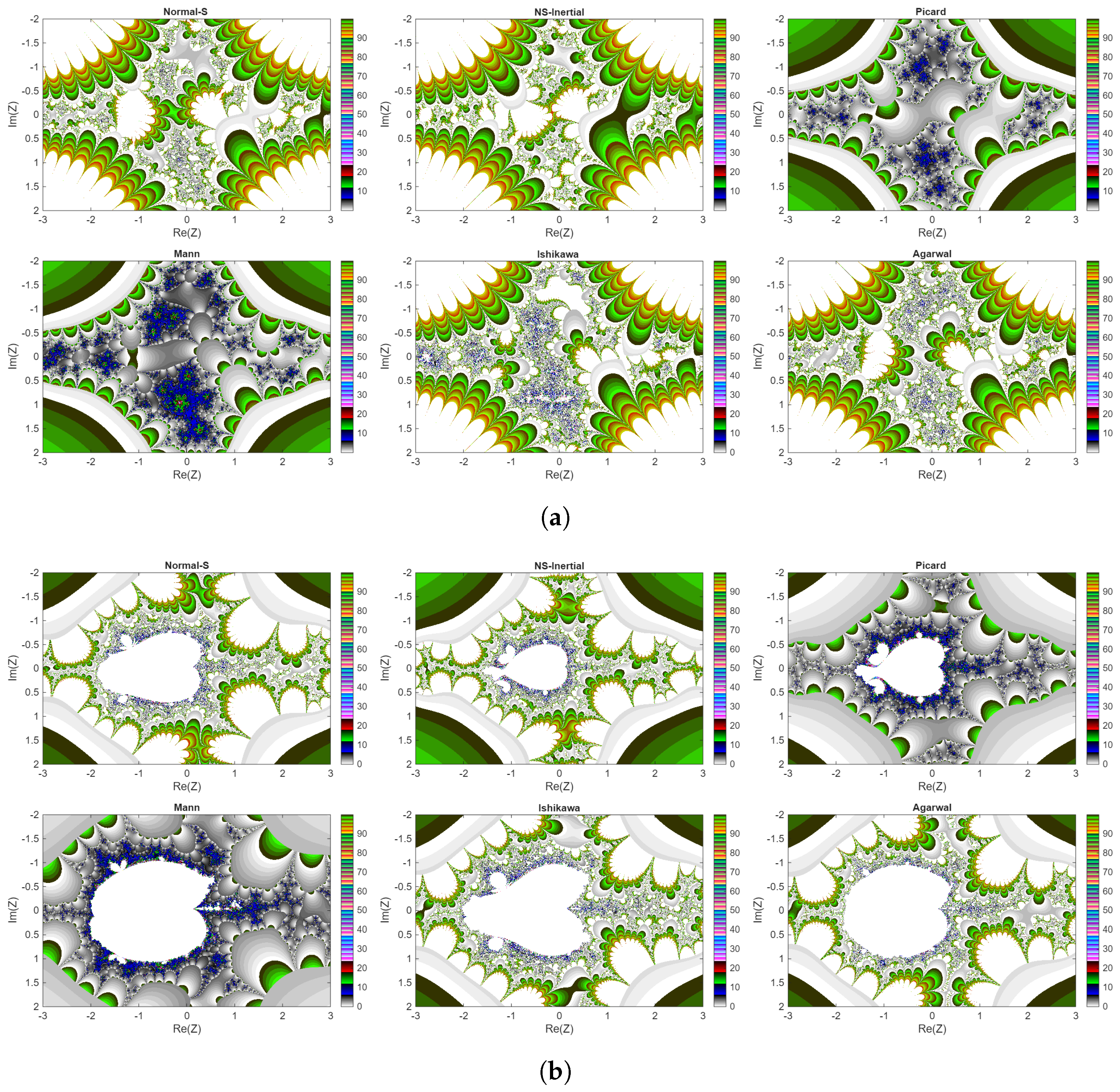
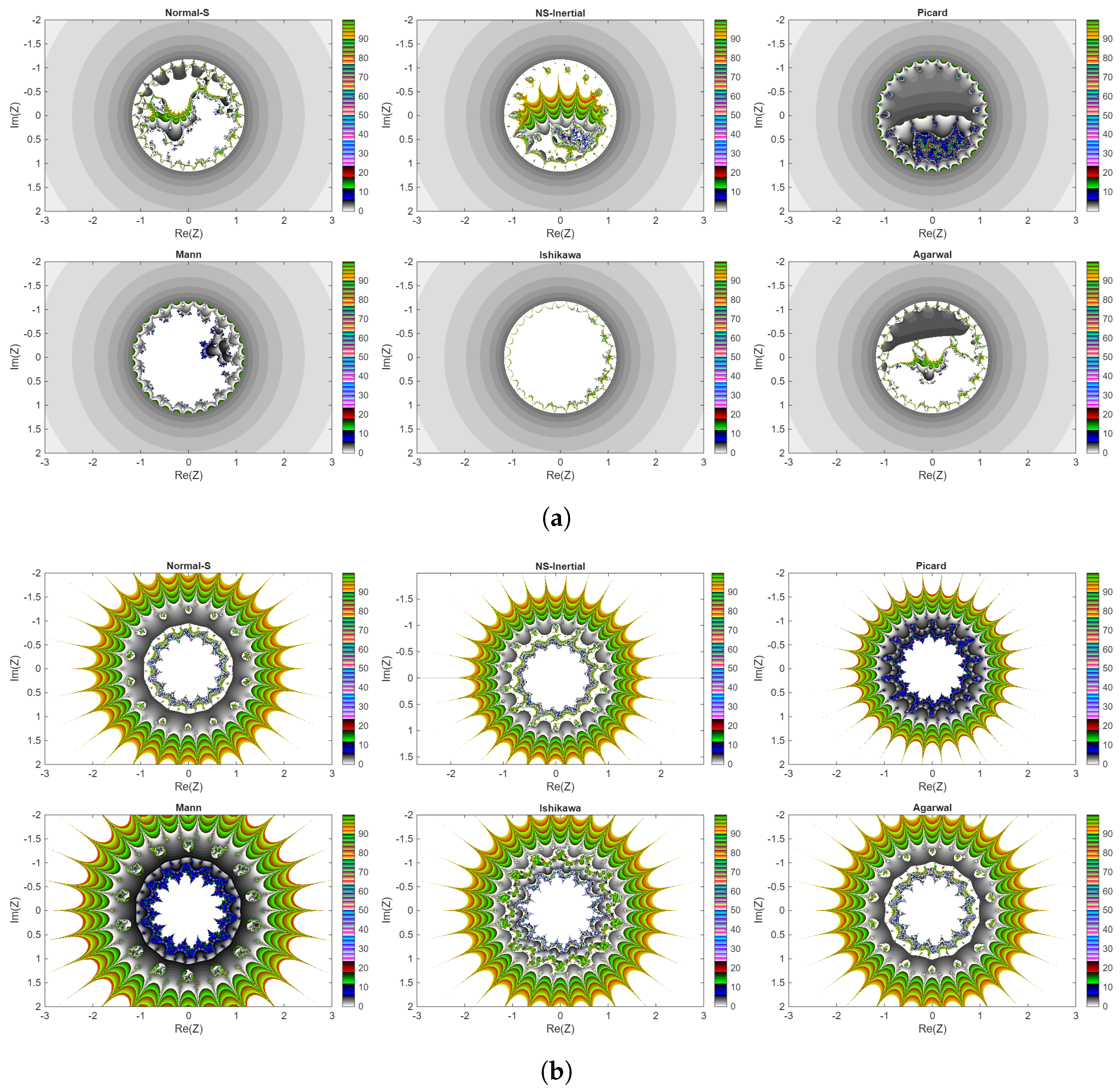
In Figure 14, the Julia set and Mandelbrot-type fractals are generated using the parameter values $c=0.8+0.86i$, $a=-0.4+0.3i$, $\tau =0.8$, $u_1=0.40$, $\alpha =0.70$, $\beta =0.40$, and $n=2$. For the NS inertial-type iteration algorithm, the inertia parameter is chosen as $\mu =0.80$. The resulting fractal images reveal interesting geometric patterns, demonstrating that different fixed point iteration algorithms applied to the same nonlinear complex function can produce significantly different fractal structures.

Figure 14. Fractal structures generated from the complex function $T\left(z\right)=\sin \left(z^n\right)+az+c$ using different fixed point iteration algorithms in the complex plane for the parameters $\alpha =0.70$, $\beta =0.40$, $\mu =0.80$, and $n=2$. (a) Julia set; (b) Mandelbrot.

In Figure 15, the Julia set and Mandelbrot-type fractals are generated using the parameter values $c=0.8+0.86i$, $a=-0.4+0.3i$, $\tau =0.8$, $u_1=0.40$, $\alpha =0.70$, $\beta =0.80$, and $n=3$. For the NS inertial-type iteration algorithm, the inertia parameter is chosen as $\mu =0.30$.

Figure 15. Fractal structures generated from the complex function $T\left(z\right)=\sin \left(z^n\right)+az+c$ using different fixed point iteration algorithms in the complex plane for the parameters $\alpha =0.70$, $\beta =0.80$, $\mu =0.30$, and $n=3$. (a) Julia set; (b) Mandelbrot.

In Figure 16, the Julia set and Mandelbrot-type fractals are generated using the parameter values $c=0.8+0.86i$, $a=-0.4+0.3i$, $\tau =0.8$, $u_1=0.40$, $\alpha =0.70$, $\beta =0.80$, and $n=5$. For the NS inertial-type iteration algorithm, the inertia parameter is chosen as $\mu =0.30$.

Figure 16. Fractal structures generated from the complex function $T\left(z\right)=\sin \left(z^n\right)+az+c$ using different fixed point iteration algorithms in the complex plane for the parameters $\alpha =0.70$, $\beta =0.80$, $\mu =0.30$, and $n=5$. (a) Julia set; (b) Mandelbrot.

In Figure 17, the Julia set and Mandelbrot-type fractals are generated using the parameter values $c=0.8+0.86i$, $a=0.00+0.00i$, $\tau =0.80$, $u_1=0.40$, $\alpha =0.70$, $\beta =0.80$, and $n=5$. For the NS inertial-type iteration algorithm, the inertia parameter is chosen as $\mu =0.30$.

Figure 17. Fractal structures generated from the complex function $T\left(z\right)=\sin \left(z^n\right)+az+c$ using different fixed point iteration algorithms in the complex plane for the parameters $\alpha =0.70$, $\beta =0.80$, $\mu =0.30$, $n=5$, and different values of a. (a) Julia set; (b) Mandelbrot.

In Figure 18, the Julia set and Mandelbrot-type fractals are generated using the parameter values $c=0.8+0.86i$, $a=-0.4+0.3i$, $\tau =0.8$, $u_1=0.40$, $\alpha =0.70$, $\beta =0.80$, and $n=5$. For the NS inertial-type iteration algorithm the inertia parameter is chosen as $\mu =0.30$.

Figure 18. Fractal structures generated from the complex function $T\left(z\right)=\sin \left(z^n\right)+az+c$ using different fixed point iteration algorithms in the complex plane for the parameters $\alpha =0.70$, $\beta =0.80$, $\mu =0.30$, and $n=5$. (a) Julia set; (b) Mandelbrot.

In Figure 19, the Julia set and Mandelbrot-type fractals are generated using the parameter values $c=0.8+0.86i$, $a=-0.4+0.3i$, $\tau =0.8$, $u_1=0.40$, $\alpha =0.70$, $\beta =0.80$, and $n=2$. For the NS inertial-type iteration algorithm, the inertia parameter is chosen as $\mu =0.30$.

Figure 19. Fractal structures generated from the complex function $T\left(z\right)=\sin \left(z^n\right)+az+c$ using different fixed iteration algorithms in the complex plane for the parameters $\alpha =0.70$, $\beta =0.80$, $\mu =0.30$, and $n=2$. (a) Julia set; (b) Mandelbrot.

In Figure 20, the Julia set and Mandelbrot-type fractals are generated using the parameter values $c=0.8+0.86i$, $a=0.30+0.1i$, $\tau =0.8$, $u_1=0.40$, $\alpha =0.70$, $\beta =0.80$, and $n=2$. For the NS inertial-type iteration algorithm, the inertia parameter is chosen as $\mu =0.30$.

Figure 20. Fractal structures generated from the complex function $T\left(z\right)=\sin \left(z^n\right)+az+c$ using different fixed point iteration algorithms in the complex plane for the parameters $\alpha =0.70$, $\beta =0.80$, $\mu =0.30$, $n=2$, and $a=0.3+0.1i$. (a) Julia set; (b) Mandelbrot.

In Figure 21, the Julia set and Mandelbrot-type fractals are generated using the parameter values $c=0.8+0.86i$, $a=0.3+0.1i$, $\tau =0.8$, $u_1=0.40$, $\alpha =0.70$, $\beta =0.80$, and $n=15$. For the NS inertial-type iteration algorithm, the inertia parameter is chosen as $\mu =0.30$.

Figure 21. Fractal structures generated from the complex function $T\left(z\right)=\sin \left(z^n\right)+az+c$ using different fixed point iteration algorithms in the complex plane for the parameters $\alpha =0.70$, $\beta =0.80$, $\mu =0.30$, $n=15$, and $a=0.3+0.1i$. (a) Julia set; (b) Mandelbrot.

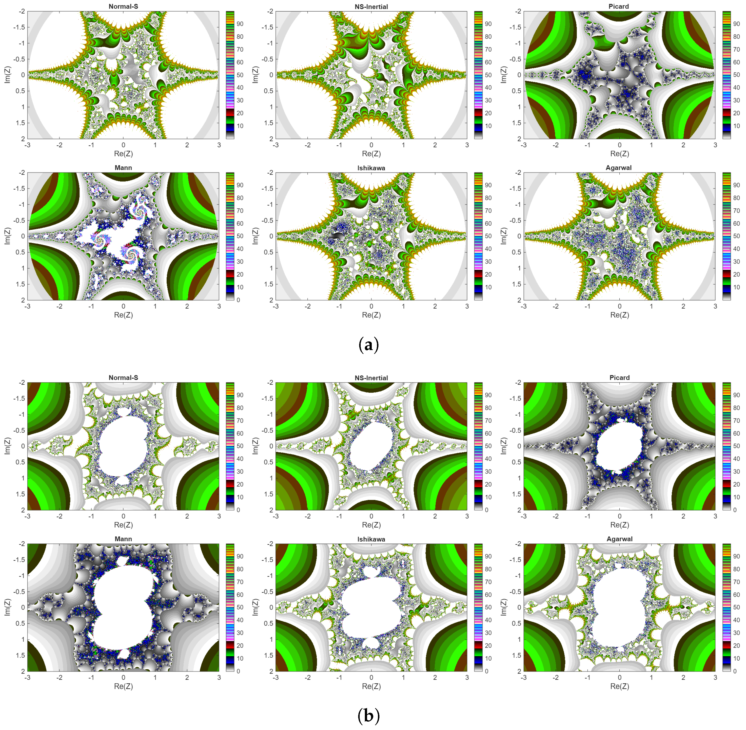
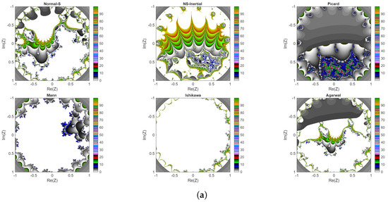
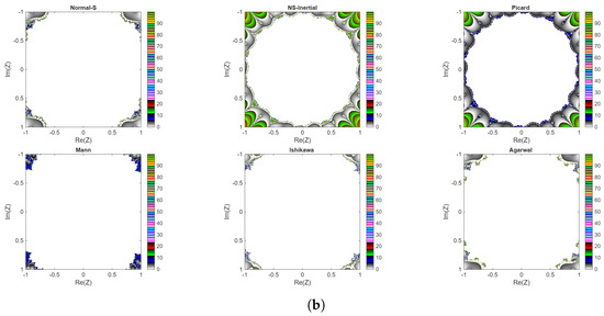
In Figure 22, the Julia set and Mandelbrot-type fractals are generated on the axes $[-2,2]x[-3,3]$ using the parameter values $c=0.8+0.86i$, $a=-0.4+0.3i$, $\tau =0.8$, $u_1=0.40$, $\alpha =0.70$, $\beta =0.80$, and $n=15$. For the NS inertial-type iteration algorithm, the inertia parameter is chosen as $\mu =0.30$.

Figure 22. Fractal structures formed on the $[-2,2]x[-3,3]$ axes for parameters $\alpha =0.70$, $\beta =0.80$, $\mu =0.30$, $n=15$, and $a=0.3+0.1i$ from the complex function $T\left(z\right)=\sin \left(z^n\right)+az+c$ using different fixed point iteration algorithms in the complex plane. (a) Julia set; (b) Mandelbrot.

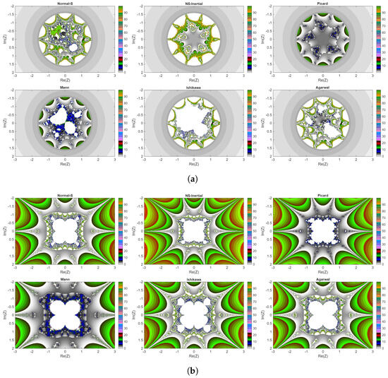
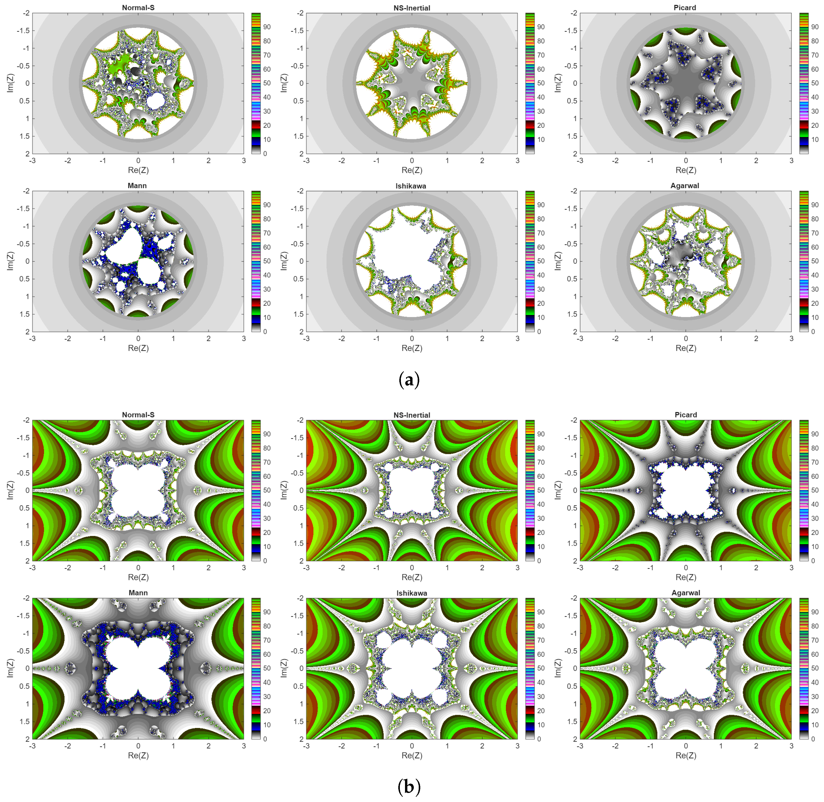
The figures presented in this study provide a comparative visual analysis of fractal structures generated from the complex function

$$T(z,n)=\sin \left(z^n\right)+az+c,$$

under different fixed point iteration algorithm. In the figures, those labeled with “(a)” correspond to Julia set fractals, while those labeled with “(b)” represent Mandelbrot-type fractals. Each image is obtained by varying the parameters a, c, and n, as well as the parameters specific to the iteration algorithms.

When all figures are considered together, it becomes clear that the resulting fractal structures are influenced not only by the parameters of the function but also, quite significantly, by the choice of iteration algorithm. Even when the same function and similar parameter ranges are used, different iteration algorithms can produce noticeably different geometric patterns.

The Picard iteration algorithm serves as a natural reference, reflecting the classical behavior of both Mandelbrot-type and Julia set fractals. The structures obtained with this algorithm exhibit the expected symmetry and highly intricate boundaries. In particular, the boundary regions display strong chaotic behavior. However, this complexity is often accompanied by irregular and abrupt transitions, which can make the overall structure appear less controlled.

The Normal S iteration algorithm produces patterns that are broadly similar to those of the Picard iteration algorithm, but with visible smoothing and expansion effects. In many of the Mandelbrot figures, the outer regions appear more spread out, while in the Julia sets, the boundaries become more fluid and less sharp. This suggests that the weighting mechanism in the iteration introduces a balancing effect on the system dynamics.

Among all the iterative algorithms, the most distinctive and compelling results are obtained with the NS inertial-type iteration algorithm. By incorporating an inertia term into the iteration algorithm, this algorithm allows the system to depend not only on the current state but also on its previous behavior. As clearly observed in both the Julia set and Mandelbrot figures, this leads to structures that are more organized, more symmetric, and visually more coherent. Particularly, boundary regions appear more evenly distributed, abrupt transitions and irregular distortions are reduced, and geometric symmetry becomes more pronounced.

In several cases, star-like or multi-fold symmetric patterns emerge, indicating that the inertial component helps guide the dynamics in a more structured way. These observations suggest that the NS inertial-type iteration algorithm does not merely generate alternative patterns but actually provides a more stable and controlled framework for exploring complex dynamical behavior. This makes it a particularly advantageous approach compared to classical methods.

The Mann iteration algorithm is characterized by smoother and more stable behavior. In the Mandelbrot-type fractal images, the main regions appear thicker and more filled, which aligns with the known property of slower but more stable convergence. In the Julia sets, this results in softer transitions and reduced fine detail.

The Ishikawa iteration, due to its two-step structure, produces more intricate boundary geometries. The figures reveal dense filament-like structures and fine-scale fractal details, indicating that this algorithm enhances the complexity of chaotic behavior, particularly near the boundaries.

The Agarwal iteration shows a behavior similar to the Ishikawa iteration algorithm but introduces more pronounced escape regions and ring-like formations in certain areas. This suggests that the mixing mechanism within the iteration modifies the system dynamics more aggressively.

As the parameters a, c, and especially n vary, the overall character of the fractals changes significantly across all algorithms. Higher values of n tend to increase symmetry and produce sharper, more structured patterns, while different values of c lead to substantial changes in the topology of the Julia sets. Despite these variations, the fractals generated by the NS inertial-type iteration algorithm consistently maintain a higher level of balance and visual coherence.

In conclusion, these figures demonstrate that fixed point iteration algorithms play a crucial role not only in convergence behavior but also in shaping the geometric and visual properties of fractal structures. Among the algorithms considered, the NS inertial-type iteration algorithm stands out due to its ability to produce more stable, symmetric, and well-structured patterns, making it a powerful and promising tool for the study of complex dynamical systems.

6. Conclusions

In this paper, we have developed an NS inertial-type iteration algorithm tailored to almost contraction mappings, a broad class that encompasses many well-known contractive conditions. By carefully designing an adaptive inertial parameter that combines the momentum coefficient from Nesterov-type acceleration with a summability control, we have been able to prove strong convergence of the algorithm under minimal assumptions. The analysis provides explicit a posteriori error estimates, demonstrates asymptotic equivalence with the classical Normal S iteration, and establishes weak $w^2$—stability as well as a sharp data dependence bound. These theoretical contributions fill a gap in the literature, as inertial algorithms had not previously been systematically investigated for almost contractions. The practical value of the proposed algorithm is underscored by two challenging applications. In image deblurring, the NS inertial-type iteration achieves a rapid initial decrease of the objective function, stable reduction in successive differences, and consistently higher PSNR values compared to several classical fixed point algorithms. In fractal generation, it yields more extensive and orderly basins of attraction and improved stability in chaotic regions, while the escape radius is

$$R_1={\left({\displaystyle \frac{2(1+|a\left|\right)}{|{\tau }_1|}}\right)}^{{\displaystyle \frac{1}{n-1}}},R_2={\left({\displaystyle \frac{2(1+|a\left|\right)}{|{\tau }_1\left|\right|{\tau }_2|}}\right)}^{{\displaystyle \frac{1}{n-1}}},$$

$$R=\max \left(\left|c\right|,R_1,R_2\right).$$

This variant further refines the visual quality of Julia and Mandelbrot sets. Collectively, the results demonstrate that the NS inertial-type algorithm is not only theoretically sound but also computationally attractive, offering a robust and versatile tool for solving a wide range of problems in fixed point theory and beyond.

References

- Banach, S. Sur les opérations dans les ensembles abstraits et leur applications aux équations intégrales. Fund. Math. 1922, 3, 133–181. [Google Scholar] [CrossRef] [Scilit]
- Osilike, M.O. Stability results for fixed point iteration procedures. J. Niger. Math. Soc. 1995, 14–15, 17–29. [Google Scholar]
- Berinde, V. Approximating fixed points of weak contractions using the Picard iteration. Nonlinear Anal. Forum 2004, 9, 43–53. [Google Scholar]
- Berinde, V. On the approximation of fixed points of weak contractive mappings. Carpathian J. Math. 2003, 19, 7–22. [Google Scholar]
- Samet, B.; Vetro, C. Berinde mappings in orbitally complete metric spaces. Chaos Solitons Fractals 2011, 44, 1075–1079. [Google Scholar] [CrossRef] [Scilit]
- Abbas, M.; Vetro, P.; Khan, S.H. On fixed points of Berinde’s contractive mappings in cone metric spaces. Carpathian J. Math. 2010, 26, 121–133. [Google Scholar]
- Altun, I.; Acar, Ö. Fixed point theorems for weak contractions in the sense of Berinde on partial metric spaces. Topol. Appl. 2012, 159, 2642–2648. [Google Scholar] [CrossRef] [Scilit]
- Karakaya, V.; Atalan, Y.; Doğan, K.; Bouzara, N.H. Some fixed point results for a new three steps iteration process in Banach spaces. Fixed Point Theory 2017, 18, 625–640. [Google Scholar] [CrossRef] [Scilit]
- Ali, F.; Ali, J. Convergence, stability, and data dependence of a new iterative algorithm with an application. Comput. Appl. Math. 2020, 39, 267. [Google Scholar] [CrossRef] [Scilit]
- Gürsoy, F.; Eksteen, J.J.A.; Khan, A.R.; Karakaya, V. An iterative method and its application to stable inversion. Soft Comput. 2019, 23, 7393–7406. [Google Scholar] [CrossRef] [Scilit]
- Hacıoğlu, E. A comparative study on iterative algorithms of almost contractions in the context of convergence, stability and data dependency. Comput. Appl. Math. 2021, 40, 282. [Google Scholar] [CrossRef] [Scilit]
- Berinde, V. Iterative Approximation of Fixed Points; Springer: Berlin/Heidelberg, Germany, 2007. [Google Scholar] [CrossRef] [Scilit]
- Doğan, K.; Hacıoğlu, E.; Gürsoy, F.; Ertürk, M.; Milovanović, G.V. Convergence-equivalent DF and AR iterations with refined data dependence: Non-asymptotic error bounds and robustness in fixed point computations. Axioms 2025, 14, 738. [Google Scholar] [CrossRef] [Scilit]
- Hacıoğlu, E.; Ertürk, M.; Gürsoy, F.; Milovanović, G.V. Flexible and Efficient Iterative Solutions for General Variational Inequalities in Real Hilbert Spaces. Axioms 2025, 14, 288. [Google Scholar] [CrossRef] [Scilit]
- Hacıoğlu, E.; Gürsoy, F.; Maldar, S.; Atalan, Y.; Milovanović, G.V. Iterative approximation of fixed points and applications to two-point second-order boundary value problems and to machine learning. Appl. Numer. Math. 2021, 167, 143–172. [Google Scholar] [CrossRef] [Scilit]
- Markin, J. Continuous dependence of fixed point sets. Proc. Am. Math. Soc. 1973, 38, 545–547. [Google Scholar] [CrossRef]
- Mureşan, S. Data dependence of the fixed point set of weakly Picard operators. Stud. Univ. Babeş-Bolyai Math. 1998, 43, 79–83. [Google Scholar]
- Rus, I.A.; Petruşel, A.; Sintămărian, A. Data dependence of the fixed point set of some multivalued weakly Picard operators. Nonlinear Anal. 2003, 52, 1947–1959. [Google Scholar] [CrossRef] [Scilit]
- Espínola, R.; Petruşel, A. Existence and data dependence of fixed points for multivalued operators on gauge spaces. J. Math. Anal. Appl. 2005, 309, 420–432. [Google Scholar] [CrossRef] [Scilit]
- Olatinwo, M. Some results on the continuous dependence of the fixed points in normed linear space. Fixed Point Theory 2009, 10, 151–157. Available online: https://www.researchgate.net/publication/267075042_Some_results_on_the_continuous_dependence_of_the_fixed_points_in_normed_linear_space (accessed on 22 March 2026).
- Rus, I.A.; Petruşel, A.; Petruşel, G. Fixed Point Theory 1950–2000: Romanian Contributions; House of the Book of Science: Cluj-Napoca, Romania, 2002. [Google Scholar]
- Abbas, M.; Ali, B.; Rashid Butt, A. Existence and data dependence of the fixed points of generalized contraction mappings with applications. Rev. R. Acad. Cienc. Exactas Fís. Nat. Ser. A Mat. 2015, 109, 603–621. [Google Scholar] [CrossRef] [Scilit]
- Şoltuz, Ş.M. Data dependence for Mann iteration. Octogon Math. Mag. 2001, 9, 825–828. [Google Scholar]
- Şoltuz, Ş.M. Data dependence for Ishikawa iteration. Lect. Math. 2004, 25, 149–155. [Google Scholar]
- Şoltuz, Ş.; Grosan, T. Data dependence for Ishikawa iteration when dealing with contractive-like operators. Fixed Point Theory Appl. 2008, 2008, 242916. [Google Scholar] [CrossRef] [Scilit]
- Çopur, A.K.; Hacıoğlu, E.; Gürsoy, F.; Ertürk, M. An efficient inertial type iterative algorithm to approximate the solutions of quasi variational inequalities in real Hilbert spaces. J. Sci. Comput. 2021, 89, 50. [Google Scholar] [CrossRef] [Scilit]
- Çopur, A.K.; Hacıoğlu, E.; Gürsoy, F.; Milovanović, G.V. Exploring the potential of inertial type algorithms in solving coincidence point/value problems: Theoretical analysis and practical applications. Filomat 2025, 39, 10205–10233. [Google Scholar]
- Shehu, Y.; Gibali, A.; Sagratella, S. Inertial projection-type methods for solving quasi-variational inequalities. J. Optim. Theory Appl. 2020, 184, 877–894. [Google Scholar] [CrossRef] [Scilit]
- Beck, A.; Teboulle, M. A fast iterative shrinkage-thresholding algorithm for linear inverse problems. SIAM J. Imaging Sci. 2009, 2, 183–202. [Google Scholar] [CrossRef] [Scilit]
- Attouch, H.; Peypouquet, J. The rate of convergence of Nesterov’s accelerated forward-backward method. SIAM J. Optim. 2016, 26, 1824–1834. [Google Scholar] [CrossRef] [Scilit]
- Sahu, D.R. Applications of S iteration process to constrained minimization problems and split feasibility problems. Fixed Point Theory 2011, 12, 187–204. [Google Scholar]
- Mann, W.R. Mean value methods in iteration. Proc. Am. Math. Soc. 1953, 4, 506–510. [Google Scholar] [CrossRef]
- Ishikawa, S. Fixed point by a new iteration method. Proc. Am. Math. Soc. 1974, 44, 147–150. [Google Scholar] [CrossRef]
- Agarwal, R.P.; O’Regan, D.; Sahu, D.R. Iterative construction of fixed points of nearly asymptotically nonexpansive mappings. J. Nonlinear Convex Anal. 2007, 8, 61–79. [Google Scholar]
- Cardinali, T.; Rubbioni, P. A generalization of the Caristi fixed point theorem in metric spaces. Fixed Point Theory 2010, 11, 3–10. [Google Scholar]
- Timis, I. On the weak stability of Picard iteration for some contractive type mappings and coincidence theorems. Int. J. Comput. Appl. 2012, 37, 9–13. [Google Scholar] [CrossRef] [Scilit]
- Harder, A.M.; Hicks, T.L. Stability results for fixed point iteration procedures. Math. Jpn. 1988, 33, 693–706. [Google Scholar]
- Liu, Q. A convergence theorem of the sequence of Ishikawa iterates for quasi-contractive mappings. J. Math. Anal. Appl. 1990, 146, 301–305. [Google Scholar] [CrossRef] [Scilit]
- Mandelbrot, B. The Fractal Geometry of Nature; W. H. Freeman: New York, NY, USA, 1983. [Google Scholar]
- Fatou, P. Sur les équations fonctionnelles. Bull. Soc. Math. Fr. 1919, 47, 161–271. [Google Scholar] [CrossRef] [Scilit]
- Julia, G. Mémoire sur l’itération des fonctions rationnelles. J. Math. Pures Appl. 1918, 8, 47–245. [Google Scholar]
- Kalantari, B. Method of Creating Graphical Works Based on Polynomials. U.S. Patent 6,894,705, 17 May 2005. [Google Scholar]
- Kotarski, W.; Gdawiec, K.; Lisowska, A. Polynomiography via Ishikawa and Mann iterations. In Advances in Visual Computing; Bebis, G., Boyle, R., Parvin, B., Koracin, D., Fowlkes, C., Wang, S., Choi, M.-H., Mantler, S., Schulze, J., Acevedo, D., et al., Eds.; Lecture Notes in Computer Science; Springer: Berlin/Heidelberg, Germany, 2012; Volume 7431, pp. 305–313. [Google Scholar] [CrossRef] [Scilit]
- Kwun, Y.C.; Tanveer, M.; Nazeer, W.; Gdawiec, K.; Kang, S.M. Mandelbrot and Julia sets via Jungck-CR iteration with s-convexity. IEEE Access 2019, 7, 12167–12176. [Google Scholar] [CrossRef] [Scilit]
- Gdawiec, K. Fractal patterns from the dynamics of combined polynomial root-finding methods. Nonlinear Dyn. 2017, 90, 2457–2479. [Google Scholar] [CrossRef] [Scilit]
- Tanveer, M.; Nazeer, W.; Gdawiec, K. On the Mandelbrot set of zp+log(ct) via the Mann and Picard–Mann iterations. Math. Comput. Simul. 2023, 209, 184–204. [Google Scholar] [CrossRef] [Scilit]
- Şahan, T.; Atalan, Y. Novel escape criteria for complex-valued hyperbolic functions through a fixed point iteration method. AIMS Math. 2025, 10, 1529–1554. [Google Scholar] [CrossRef] [Scilit]
- Antal, S.; Tomar, A.; Prajapati, D.J.; Sajid, M. Fractals as Julia Sets of Complex Sine Function via Fixed Point Iterations. Fractal Fract. 2021, 5, 272. [Google Scholar] [CrossRef] [Scilit]
Disclaimer/Publisher’s Note: The statements, opinions and data contained in all publications are solely those of the individual author(s) and contributor(s) and not of MDPI and/or the editor(s). MDPI and/or the editor(s) disclaim responsibility for any injury to people or property resulting from any ideas, methods, instructions or products referred to in the content. |
© 2026 by the authors. Licensee MDPI, Basel, Switzerland. This article is an open access article distributed under the terms and conditions of the Creative Commons Attribution (CC BY) license.