


Abstract
We propose a robust method for outlier detection in functional data analysis. This approach uses the robust Minimum Covariance Determinant estimator to compute the Mahalanobis distance applied to functional principal component scores. The main contribution of this research is the detection of outlier curves using the robust covariance matrix of functional principal components, in contrast to existing methods that use principal components on the discrete dataset. The proposed method is practical because it considers the entire functional form of the data, through their functional principal components, providing a comprehensive analysis that can detect anomalies across the entire functional range. A simulation study compares this approach with existing methods to evaluate their performance, followed by applications to El Niño Sea Surface Temperature data and SCImago Journal Rank data. The results show that the proposed method provides greater accuracy, demonstrating its effectiveness in detecting outlier curves.
Keywords:
functional data analysis; outlier detection; functional principal component analysis; minimum covariance determinant estimator; robust Mahalanobis distance MSC:
62R10; 62H25
1. Introduction
The use of information systems involves collecting and analyzing data generated by sensors or transactional systems. Functional data refers to information observed continuously or at several discrete points over a time interval. Functional Data Analysis (FDA) focuses on the statistical analysis of functions as units of analysis, allowing the discovery of complex patterns and characteristics implicit in functional data [1]. Consequently, classic statistical techniques, such as dimension reduction, data classification and regression, are extended to be applied to the study of functional data.
In statistical analysis, an important task is the detection of outlier observations. These could influence the result of an analysis and distort the conclusions. Outliers are values in a dataset that are significantly different from most observations, probably due to errors in the data or unusual events within the domain of study [2]. In FDA, outliers are curves with different characteristics from the functions in the dataset. To detect outlier curves, it is necessary to analyze the discrete values of each observation and consider them as curves. Therefore, while a curve may not be abnormal at a specific point, it may be across its entire functional set [2].
Various approaches exist for detecting outlier curves. One approach is based on functional depth, which evaluates the centrality of curves within a dataset. A higher depth value is assigned to curves closer to the center, while a lower depth value is assigned to curves at the extremes. Curves with depth values below a specific threshold are classified as outliers [2]. Among depth methods are depth based on functional medians [3], depth based on functional modes [4], and functional boxplot [5], which uses depth bands [6]. Other methods focus on identifying outlier observations through Principal Component Analysis (PCA). In the PCA context, some methods include the functional bagplot [7] and functional highest density region (HDR) boxplot [7], which are implemented over the first two robust principal components of functional curves. In addition, the Integrated Squared Error (ISE) method [8] is applied to the k robust principal components, usually two. Practical visual tools for identifying functional outlier observations that are not obvious when applying mathematical models include the functional boxplot, functional bagplot, functional HDR boxplot, and other graphical methods such as the outliergram [9], functional outlier map [10], and magnitude-shape plot [11].
Detecting outlier observations in multivariate datasets is a complex task that requires robust techniques. These outlier observations can be identified using Mahalanobis distance (MD) in a multidimensional space, considering the covariance of the dataset [12,13]. The robustness of the analyses is obtained by the use of a robust covariance matrix through methods that are less susceptible to outliers [14], such as the Minimum Covariance Determinant (MCD) or the Minimum Volume Ellipsoid (MVE) estimators [15,16]. Sawant et al. [17] proposes a Functional Principal Component Analysis (FPCA) method that uses a robust covariance matrix for data dimension reduction and outlier detection. Oguamalam et al. [18] introduce the Minimum Regularized Covariance Trace (MRCT) method for robust covariance estimation. The MRCT uses a subset-based strategy that gives greater weight to observations with higher centrality according to their Mahalanobis distance.
It is important to note that while the above methods utilize robust techniques for functional data, they may not necessarily be applied to continuous data. Therefore, it is necessary to analyze outlier detection methods that consider observations as curves and use robust techniques based on FPCA. This research introduces a technique for identifying functional outliers using the robust MCD estimator. The main contribution of this study is to detect functional outliers using the robust covariance matrix over functional principal components. The proposed method differs from existing methods based on PCA approaches, which focus on the first two principal components or work with discrete datasets. This paper is organized as follows: Section 2 describes existing methods based on PCA and FPCA. The new proposal for functional outlier detection is detailed in Section 3. In Section 4, an extensive simulation study is conducted to compare the performance of the proposed method with existing methods. Finally, Section 5 applies the proposed methodology to two real datasets, El Niño Sea Surface Temperature data and SCImago Journal Rank data.
2. Functional Outlier Detection Methods Based on PCA
In this section, we introduce the mathematical fundamentals of FDA and subsequently describe the existing methods based on PCA and FPCA for the detection of outlier curves in FDA.
2.1. Fundamentals of Functional Data
Functional Data Analysis (FDA) focuses on the statistical treatment of data represented as functions, which can be regarded as random elements taking values in a Hilbert space such as , the space of square-integrable functions over an interval , or equivalently as realizations of a stochastic process. A functional data set consists of curves generated by a functional variable , , taking values in a functional space such as . In practice, each curve is observed only at a finite grid of points , since the underlying mathematical form of the function cannot be directly observed [1].
Let denote the Hilbert space of square-integrable functions,
equipped with the inner product
Given a sample , the functional mean is defined as
and the covariance surface is given by
Discrete observations can be transformed into functional data using basis expansion techniques [1]. A basis is a collection of functions such that any function in the space can be approximated by a linear combination of these K functions. Thus, a functional observation can be expressed as
where are the basis coefficients associated with . When this representation holds for all curves , the sample is considered to lie in the K-dimensional subspace spanned by the basis functions .
To recover the functional form of a curve from its discrete observations , it is typically assumed that the observations are contaminated with measurement error. Consequently, least squares estimation is commonly used to obtain the basis coefficients [1]. Let denote the vector of basis functions. Then Equation (2) can be written as
where . If denotes the matrix with entries , the least squares estimator of the coefficient vector is
which minimizes the mean squared error
Selecting a particular basis or dimensionality does not, by itself, determine whether a curve should be considered an outlier. This classification depends on the curve’s intrinsic characteristics relative to the rest of the sample. When all curves are represented using a common basis and the same number of components, they are embedded in a shared functional space. It is within this common space that one can meaningfully assess whether a given curve deviates substantially from the others and should therefore be regarded as an outlier.
2.2. Functional Principal Component Analysis
In a dataset with n observations, each consisting of p variables, PCA seeks to identify a reduced number of factors q that explain approximately the same amount of information as the original p variables . The first component captures the greatest amount of variation in the data, the second captures the next largest amount, and so on [19]. In the functional setting, FPCA identifies a new basis of functions whose first elements contain the maximum variability.
Let , , be a sample of centered curves, and let denote the covariance operator for functions in , defined as
where is the covariance surface from Equation (1) with , without loss of generality. The j-th functional principal component score is given by the n-dimensional vector with components
where is the j-th solution of the integral equation
The parameter and the function are known as the eigenvalue and eigenfunction of the covariance operator. Due to the properties of the covariance function, and using the basis expansion methodology described in Section 2.1, there exist K solutions to Equation (3), given by the pairs , satisfying
and the eigenfunctions form an orthogonal set in . Moreover, represents the variance of the j-th functional principal component score. Each curve can be approximated using a reduced set of functional principal components as
(see [1]). The proportion of variance explained by the first L functional principal components is given by
Expression (5) enables the curves to be approximated with arbitrary precision through their functional principal components. In this representation, the scores capture the stochastic variability within the sample of curves, whereas the eigenfunctions encode their underlying functional structure. Consequently, any statistical procedure applied to the set of scores can be interpreted as operating on the full functional form of the curves.
2.3. Functional Bagplot
The univariate boxplot for a scalar variable [20] provides information about data distribution, identifying the median , the quartiles ( the value greater than 25% and the value greater than 75% of the ordered data), and the interquartile range of data distribution. The bivariate bagplot [21] extends the concept of the univariate boxplot, it includes a bag that contains 50% of the observations and a fence that separates inliers from outliers. In a univariate boxplot, the central element is the median, and the outliers are those observations outside the interval . On the other hand, in a bivariate bagplot, the central point is the Tukey median and the fence is obtained by inflating the bag by a factor [21]. Observations that fall outside the fence are identified as outliers.
Traditional boxplots represent and summarize unidimensional data, while functional bagplots are applied to sets of functions or curves. The functional bagplot [7] adapts the bivariate bagplot for functional data. This adaptation involves analyzing the first two robust principal component scores of the functional curves. Considering a set of the functional curves of , the principal component scores are obtained from the robust principal component scores of the discretized curves through Projection–Pursuit (PP) robust PCA algorithm [22]. The first two score vectors and are then evaluated using methods of bivariate depth. Obtained scores are ordered based on Tukey’s halfspace location depth [23]. Let be the observation associated with the i-th largest depth value, where is considered as a median curve and the curves progressively extend outward to the outermost curve .
In a functional bagplot, the bag includes 50% of the curves with the deepest values located in the inner region. The outer region is defined by the set of curves associated with points within the bivariate fence region. This fence is created by inflating the bag by a factor of and contains 99% of the curves. Curves outside this fence are identified as outliers.
2.4. Functional HDR Boxplot
The Highest Density Regions (HDR) are regions in probability space where the concentration of observations is particularly high compared to others. These regions are characterized by a relatively small set containing the greater probability in the sample space, focusing on critical regions. A kernel density estimator [24] is employed to determine the number of modes in the observation distribution to determine the areas of probability concentration.
The bivariate HDR boxplot uses the 50% HDR to display IQR, and its bounded region corresponds to the 99% HDR. All observations that exceed the 99% HDR level are considered outliers. Functional HDR [7] is a generalization of the HDR boxplot. This method determines probability concentration regions using a bivariate kernel density estimate. This estimate is applied to the first two vectors of scores and , which are obtained from the robust principal component scores of the discretized curves , using the PP robust PCA algorithm [22]. The bivariate kernel density, denoted as , is calculated as follows:
with that denotes a set of bivariate points. The kernel function is scaled by the bandwidth for the i- dimension and the kernel estimate is defined as . The values are ordered descendingly. Let represent the observation associated with the i- highest value of , where denotes the curve with the highest density, defined as the modal curve. In contrast, the curve corresponds to the most unusual curve.
2.5. Integrated Squared Error
The Integrated Squared Error (ISE) method [8] uses robust PCA based on the weighted principal component method and the reflection-based algorithm for PCA (RAPCA). The RAPCA algorithm, based on PP methods, maximizes a robust measure and searches for the direction in which the projected observations have maximal variance [25].
ISE first uses a nonparametric smoothing method to estimate for . Then, each fitted curve is decomposed by a basis function expansion using
where is a measure of location of , is a set of basis functions and is normally distributed with . Using the RAPCA algorithm, the initial values for and are obtained.
The ISE for each observation is defined as:
which provides a measure of the precision of the principal component approximation for i-th observation, with K denoting the number of components (typically two), represent a set of principal component functions and are their associated scores.
If follows a normal distribution, then has a distribution and . The probability that is approximately , where denotes the distribution function of the standard normal distribution. Here, s represents the median of and is a tuning parameter used to control the level of robustness.
Table 1 summarizes the main characteristics of the existing methods based on PCA and FPCA to be applied in the study for functional outlier detection.
Table 1.
Summary of outlier detection methods for FDA based on PCA and FPCA.
3. Methodology for Functional Outliers Detection
In this section, we first describe the fundamentals of Mahalanobis distance and FPCA. Subsequently, we present the proposed method for outlier detection of curves in FDA based on robust Mahalanobis distance and FPCA.
3.1. Principles of Mahalanobis Distance
Mahalanobis distance (MD) [26] is a measure used to determine the distance between observations in a multivariate space, considering the correlation and covariance of the data matrix. Unlike the Euclidean distance (ED), which considers all distances between observations equally important and uncorrelated with a circular envelope, the MD has distances towards the center point with an elliptic envelope [27].
The MD towards the mean of the data is calculated as
where represents the i-th observation, is the mean of the data, is the transpose operator and ∑ denotes the variance-covariance matrix of the dataset.
A characteristic inherent to the MD is that their distances to the data center follow a distribution with p degrees of freedom, where X is a p-dimensional vector that follows a multivariate normal distribution [28]. Here, represents the critical value, commonly corresponding to the 97.5% quantile of the distribution. The observations with distances above the cutoff point of the distribution are categorized as outliers [29].
3.2. Robust Mahalanobis Distance
The robust MD is a modified version of the standard MD, designed to reduce sensitivity to outliers [14]. Different methods have been developed to estimate the robust Mahalanobis distance, mainly using the robust covariance matrix with the MCD estimator [15,16]. The MCD estimator was proposed by Rousseeuw [15] for detecting multivariate outliers. Its goal is to find h observations (sub-samples of size h), where the most central sub-sample is identified as having the lowest variability among the observations. This is determined by a covariance matrix with the minimum determinant value. A sub-sample is selected, obtaining sub-samples of size h. The parameter h determines the robustness of the MCD estimator and allows the determination of a breakdown value when
where , denotes the integer part of the quotient, n is the number of observations and p is the number of variables. When selecting sub-samples with , it has a breakdown point of 0.5 (MCD 50) and with , it has a breakdown point of 0.25 (MCD 75). MCD 50 and MCD 75 are commonly used, but MCD 75 has better efficiency [16,30,31,32].
The choice of h in the MCD estimator determines its finite sample breakdown point and statistical efficiency [33]. Setting MCD50 achieves the maximal breakdown point of 50%, providing optimal resistance to contamination [33]. In contrast, selecting MCD75 reduces the breakdown point to 25%, but substantially improves efficiency under multivariate normality [14]. Consequently, MCD50 can be viewed as a specification that prioritizes robustness, whereas MCD75 represents a compromise between robustness and efficiency that is particularly suitable when contamination is expected to be moderate [34,35].
Hyndman and Shang [7] apply the robust MD to functional curves, using the MCD estimator for calculating the covariance matrix with a breakdown value of . The method evaluates the discrete matrix of curves , defining outliers as those curves whose distances exceed the cutoff point, with an confidence level.
3.3. Outlier Detection Method Based on Robust Mahalanobis Distance and FPCA
In the context of dimensionality reduction, robust methods can be employed to define the robust covariance matrix. In FDA, several robust FPCA methods exist, which are less sensitive to outlier curves. Sawant et al. [17] extend robust PCA (ROBPCA and BACONPCA methods) to FPCA to identify linear combinations of the original variables that capture the majority of the information while simultaneously detecting functional outliers. These methods are applied to the functional coefficients from Equation (2), integrating concepts of PP and the MCD estimator. In the MCD, the methods choose a value of or greater than with . Outlier observations are classified using MD, with a cutoff defined by the distribution with p degrees of freedom and a significance level of .
Under the assumption of multivariate normality, the squared Mahalanobis distances asymptotically follow a distribution with p degrees of freedom [36]. Therefore, cutoff values based on the 97.5% and 99% quantiles provide statistically controlled thresholds for outlier detection, corresponding to type I error rates of 2.5% and 1%, respectively [12]. These levels represent a principled balance between sensitivity and specificity and are widely adopted in robust multivariate analysis, particularly when robust estimators such as the MCD are employed under certain conditions [37,38].
Since outlier curves are not necessarily anomalous at a specific time point, but over their entire functional space, it is necessary to analyze the curves across their continuous space. Therefore, the analysis of outlier curves should be evaluated on continuous data and not exclusively on a discrete matrix. The proposed method for functional outlier detection based on the robust MD involves dimension reduction through FPCA followed by the calculation of the robust distance. This procedure is detailed below:
- Step 1. Given a discrete set of observations, transform the discrete dataset into functional data using basis functions, such as Fourier or [1], to obtain the functional curves expressed as Equation (2).
- Step 2. From Equation (4), obtain the principal components and the , principal component scores through functional principal component decomposition. The value of L is determined to capture a sufficiently significant amount of variability.
- Step 3. Using Equation (6), calculate the robust MD distance from a reduced set of L functional principal component scores that cumulates a certain percentage of explained variability (95% or 99%). Robust distances are calculated using the MCD estimator.
- Step 4. Since the MD follows a distribution with L degrees of freedom, establish an cutoff point. Curves with a robust MD distance exceeding the values are classified as outliers.
In this study, for step 1, we use third-order basis functions to transform the discrete dataset into functional data. In step 2, L values are determined such that the first L functional principal components accumulate 95% and 99% of variability. In step 3, we use the MCD 50 and MCD 75 estimators. Step 4 employs alpha values with a significance level of 97.5% and 99%.
4. Simulation Studies
This section presents an simulation study comparing the proposed method with existing approaches for functional outlier detection. Six mathematical models are defined, and one hundred simulations are conducted to analyze the behavior of each method and evaluate how each model responds to various conditions.
4.1. Functional Models
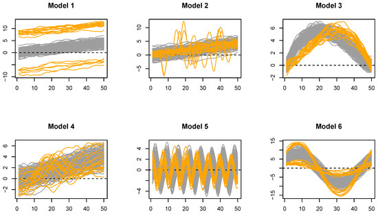
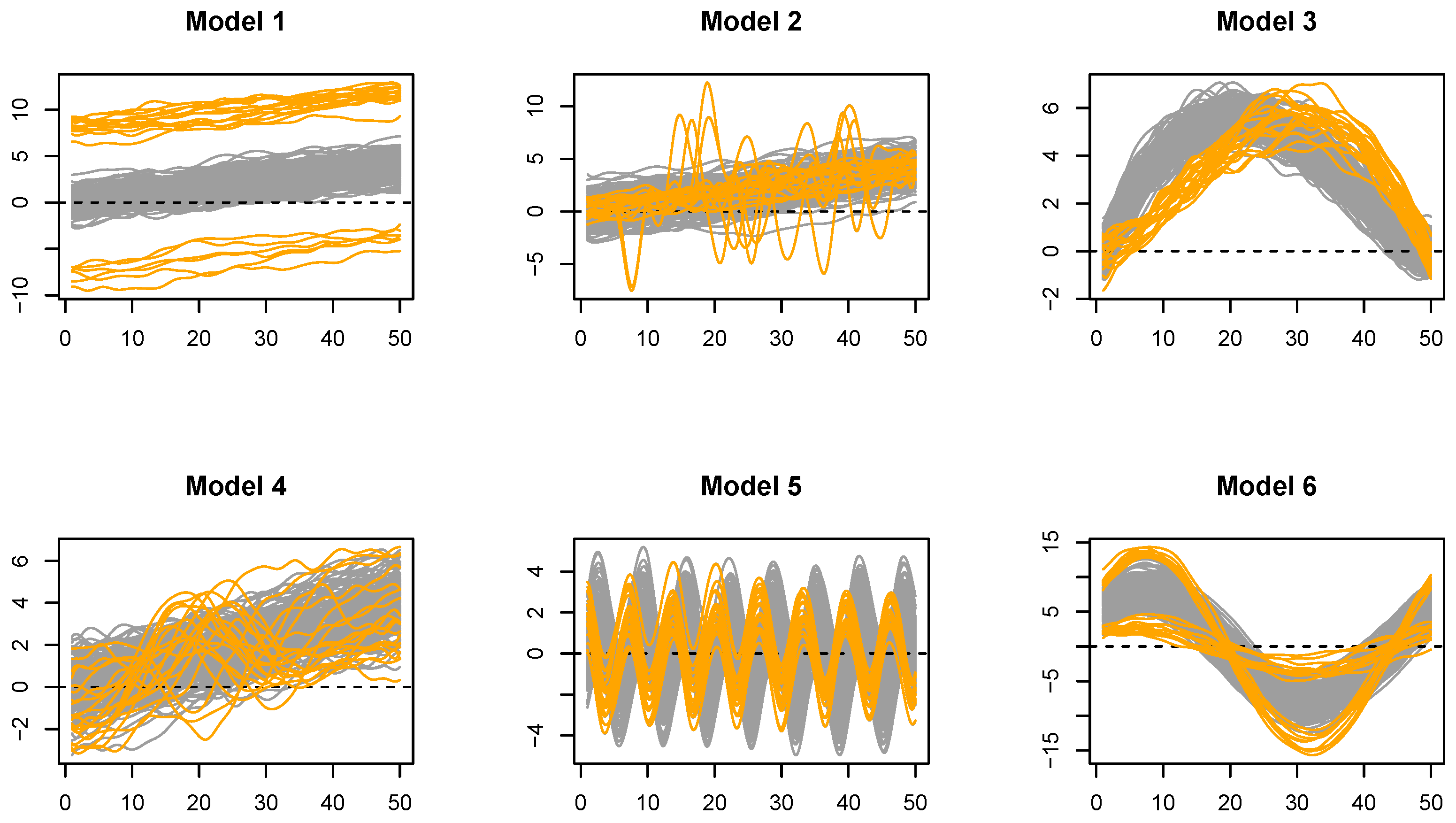
To evaluate the robustness of the proposed method, six mathematical models are considered in the development of this study (see Figure 1). These models are obtained from the library in R, which compiles various existing models from the literature within the FDA.
Figure 1.
Models simulation with observations and contamination rate (10%). Curves generated from the main model (gray) and the contamination model (orange).
- Model 1: Characterized by linearly increasing functions and the outlier observations deviating from the non-outlier curves. The primary model is . The contaminated data follows the model , where , is a Gaussian process with zero mean and covariance function , and with equal probabilities for 1 and −1 ().
- Model 2: It is characterized by linearly increasing functions. The model generates outlier values that are significant only for a portion of the domain of the functional data. The main model is . The contaminated data follows the model , where I represents the indicator function, T is a uniformly distributed random variable in the interval and l is a constant that specifies the extent to which outlier values are displaced from the mean function in the domain.
- Model 3: The model generates displaced outlier values inversely related to the original observations in the domain of the model. The main model is . The contaminated data follows the model .
- Model 4: The model generates linearly increasing functions. The main model is . The contaminated data follows the model , where follows a Bernoulli distribution with probability and v follows a uniform distribution in the interval .
- Model 5: They form a group of periodic functions. The main model is . The contaminated data have the model , where is contamination coefficient.
- Model 6: They constitute a group of periodic functions. The main model is . The contaminated data follow the model . The coefficients follow a uniform distribution in the interval ; follow a uniform distribution in the interval ; and follow a uniform distribution in the interval .
The six simulation models were designed to systematically represent distinct categories of functional anomalies commonly discussed in the literature:
- Model 1 generates shift outliers, where curves preserve the overall shape of the main process but are shifted either vertically (magnitude shift) or horizontally (phase shift).
- Model 2 represents isolated outlier, characterized by abnormal behavior within a restricted subinterval of the domain while remaining consistent with the majority pattern elsewhere. Such deviations are particularly challenging because global structure is largely preserved.
- Models 3 and 6 correspond to amplitude outliers, where curves maintain the same functional form as the bulk of the data but differ in scale or range. These represent magnitude contamination without structural deformation.
- Models 4 and 5 introduce a shape outlier, characterized by structural deformation in a limited region of the domain, affecting curvature or local dynamics without necessarily producing large pointwise deviations.
Collectively, these models cover magnitude, amplitude, localizedness, shape, and displacement-based contamination mechanisms, thus providing a structured evaluation of detection power across typologies [39]. The goal of the simulation design is to cover representative contamination mechanisms rather than exhaustively enumerate all possible deformation types.
4.2. Simulation Design
The simulations compare different outlier detection methods for functional data, including evaluation of the proposed method. We focus on the ISE [8], functional bagplot [7] and functional HDR boxplot [7] from the rainbow library developed in R. Additionally, the evaluation includes robust MD methods based on MCD, such as MCD 50 and MCD 75.
For each model considered in this study, one hundred simulations are conducted to analyze the behavior of each method and evaluate how each model responds to various conditions. A sample size of is defined, with three different values selected for the contamination rate: and . For each method, two evaluation metrics are presented:
- True Positive Rate : The proportion of correctly identified outliers, calculated as the ratio between the number of true outliers correctly detected and the total number of outliers in the sample (sensitivity).
- False Positive Rate : The proportion of non-outliers incorrectly identified as outliers, calculated as the number of outliers incorrectly identified divided by the total number of non-outlier observations in the sample. (false detection rate).
For the standard MD, MCD 50, and MCD 75 methods, we apply a number L of functional components that account for 95% and 99% of variability. We also establish the cutoff point that identifies the outlier curves with a significance level of 0.975 and 0.99.
4.3. Simulation Results
The following subsection describes the results obtained from the simulation, including the mean by model of the proportion of correctly () and falsely () identified outliers. To better understand the results, the analysis is divided into three parts. The first part focuses on the standard MD method, the second on the robust MD (MCD 50 and MCD 75), and the final part covers the ISE, functional HDR boxplot and functional bagplot methods.
Table 2 and Table 3 report the results for observations under a contamination level of (5%). Table 4 and Table 5 correspond to (10%), whereas Table 6 and Table 7 present the results for (20%). For each contamination level, the performance metrics and are analyzed, and the corresponding bootstrap confidence intervals are presented to assess the variability of the estimates.
Table 2.
Mean and bootstrap confidence intervals of the proportion of correctly identified outliers () across models, for and contamination rate (5%).
Table 3.
Mean and bootstrap confidence intervals of the proportion of falsely identified outliers () across models, for and contamination rate (5%).
Table 4.
Mean and bootstrap confidence intervals of the proportion of correctly identified outliers () across models, for and contamination rate (10%).
Table 5.
Mean and 95% confidence intervals of the proportion of falsely identified outliers () across models, for and contamination rate (10%).
Table 6.
Mean and bootstrap confidence intervals of the proportion of correctly identified outliers () across models, for and contamination rate (20%).
Table 7.
Mean and bootstrap confidence intervals of the proportion of falsely identified outliers () across models, for and contamination rate (20%).
For Model 1, the methods that achieve the best performance are the robust ones (MCD 50 and MCD 75), with and metrics near to 1 and 0, respectively, across different contamination rates and combinations of k and values. In Model 2, the results of the methods are very similar for both and metrics, with the best values achieved using the standard Mahalanobis method. Model 3 shows significantly superior results for the robust methods in the metric. For model 4, the metric values are very similar in robust methods and ISE; however, it is evident that the performance of the standard Mahalanobis method deteriorates as the contamination rate c increases. Model 5 has a contamination rate of , and the results are very similar (with for robust methods and near 1 for the ISE method). At the same time, it is evident that the performance of the standard MD method deteriorates as the contamination rate c increases, although maintains stability for robust methods and ISE. Finally, Model 6 shows results that are not very precise for all methods analyzed in the simulation, with performance decreasing as the contamination rate c increases.
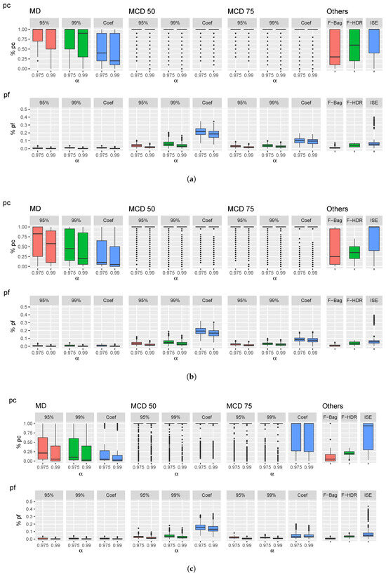
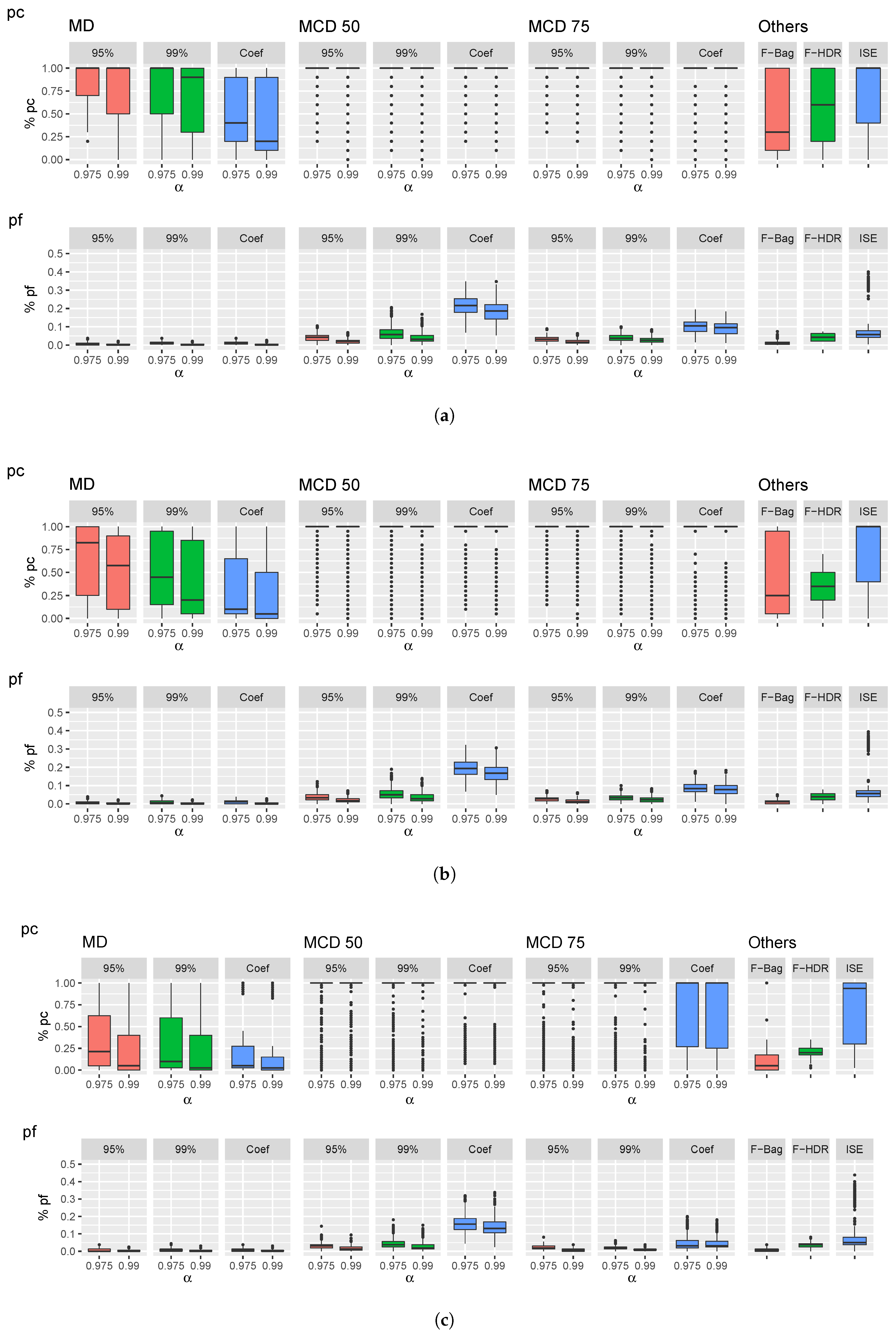
Comparing the different methods, it can be observed that for the metric, the results obtained by the robust MD are superior to the values resulting from the standard MD and significantly superior to the ISE, functional HDR boxplot and functional bagplot methods. Although the metric shows better results with the standard MD than the robust methods, the differences are not very significant. For six models, the results obtained by the ISE, functional HDR boxplot and functional bagplot methods, are significantly inferior compared to the methods based on the robust MD. We present the numerical results using boxplots illustrated in Figure 2, constructed over 300 simulations (100 simulations for each contamination rate, and ). It is evident that as the contamination rate c increases, the performance of the metric of the standard MD method significantly diminishes, with considerable dispersion in its values. In contrast, for the robust methods (MCD 50 and MCD 75), the interquartile range is centered around , with minimal dispersion; however, it exhibits observations distributed in the interval , represented as outliers in the boxplot. The interquartile range of the metric in the boxplot is kept constant across simulations for the ISE method. For the and metrics, the performance of the functional HDR boxplot and functional bagplot methods are similar to the results of the standard MD method. Finally, within the robust methods, the results obtained for the metric, using k values that capture 95% and 99% of variability in the FPCA, are equivalent to the results obtained for the functional coefficients; however, for the metric, these results exhibit the least efficiency.
Figure 2.
Boxplot of correctly and falsely identified outliers on the six models for observations and contamination values (a) , (b) and (c) . Applies to functional coefficients (coef), L functional components that capture 95% and 99% of the variability, along with cutoff of 0.975 and 0.99.
Evaluating the metrics collectively, it can be concluded that the best results are obtained by the MCD 75 estimator, with a k number of functional components that account for 95% of variability and the cutoff point that identifies the outlier curves with an . These results demonstrate consistency across the three simulations with and contamination rates.
To assess whether the number of principal components explaining 95% and 99% of the total variability is adequate for detecting and using the proposed methods, we selected, for each of the six models considered, one of the 100 simulations generated with a 5% contamination of outliers. For each model, we computed and using different numbers of principal components across the various approaches (standard MD, MCD 50 and MCD 75) and for the two values of defining the chi-square quantile threshold (0.975 and 0.99). The results are presented in Table A1–Table A6 and in Figure A1 of Appendix A. As can be observed, selecting the number of components that explain 95% or 99% of the variability yields, in nearly all cases, a of 100%, while the values remain lowest for the MCD 50 and MCD 75 methods. The results also show that moving to higher numbers of components systematically worsens the values.
5. Applications
In this section, we apply the methods analyzed in the study to two real datasets for outlier detection of functional curves. The methods to be evaluated include the ISE [8], functional bagplot [7] and functional HDR boxplot [7]. For the MCD 75 method, we used a k number of functional principal components that capture 95% of the variability. In addition, we used with value of 0.99 as cutoffs to detect outlier curves.
5.1. El Niño Sea Surface Temperature Data
The dataset corresponds to the monthly average of El Niño Sea Surface Temperature (SST), representing Pacific Ocean temperatures in the South American coastal region (coordinates West, 0– South). To replicate the rainbow example [7], the dataset to be used is obtained from the rainbow_1.4.zip library, available at https://cran.r-project.org/src/contrib/Archive/rainbow (accessed on 22 May 2024). The dataset contains values measured in , from January 1951 to December 2007. Each observation represents an annual temperature evaluated monthly. The outlier observations in the SST are the years 1982–1983 and 1997–1998 [40]. In [7], the functional HDR boxplot and functional bagplot methods correctly detect the outlier temperatures. Similarly, the ISE method detects the years 1973, 1982–1983 and 1997–1998 as outlier temperatures, with an incorrect detection for 1973.
The replicated results for functional HDR boxplot, functional bagplot and ISE methods, based on the study of [7], are shown in Table 8. The MCD 75 method correctly detects the years 1982–1983 and 1997–1998 as outlier temperatures, observations with a robust MD above the cutoff point of the are classified as outliers. The MCD 75 method, which utilizes FPCA, operates with four principal components that account for 96.39% of the variability. In contrast, the ISE method, which employs PCA, works with two principal components, accumulating 87.03% of the variability. On the other hand, the functional HDR boxplot and functional bagplot methods operate with two principal components that reach 100% of the variability, due to the inherent nature of the PP robust PCA [22] method used.
Table 8.
A comparison of outlier detection applied to El Niño SST data.
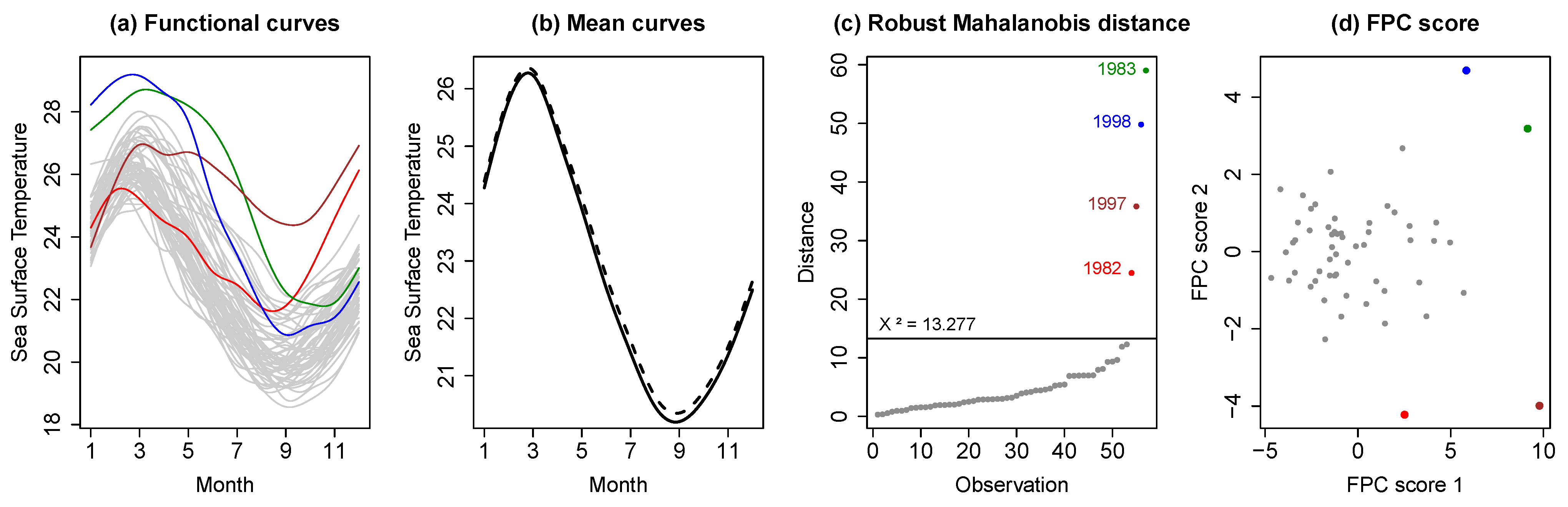
Figure 3a shows the functional curves corresponding to El Niño SST data, with the curves identified as outlier temperatures presented in colors. Mean curves with outliers (dotted line) and without outliers (continuous line) are presented in Figure 3b. The robust MD of each annual temperature with the cutoff is plotted in Figure 3c. Scatterplots of the first two functional principal components, shown in Figure 3d, reveal how the temperature outliers are distant from the non-outliers and easier to detect.
Figure 3.
The visualization of El Niño Sea Surface Temperature data. (a) Functional curves, curves colored other than gray, represent the outlier year temperatures. (b) Mean curves with outliers (dotted line) and without outliers (continuous line). (c) The robust Mahalanobis distances of each annual temperature and the cutoff. (d) Scatterplots of the FPCA scores.
5.2. SCImago Journal Rank Data
As a second example, we utilized data from the SCImago Journal Rank website, available at https://www.scimagojr.com. This platform annually calculates various metrics to evaluate and rank scientific journals in Scopus. A main metric is the SJR index, which ranks journals based on their weighted prestige and the number of citations received over a three-year period. The SCImago system organizes journals into 27 knowledge areas and each thematic area is grouped into specific categories that share common themes, simplifying the search and analysis of scientific publications by thematic field. This study examines the SJR metric values from 1999 to 2022 for the Statistics and Probability category, which is part of the Mathematics knowledge area. We focus on journals with SJR values for each year of the time interval. A total of 95 journals satisfy these criteria and are included in this functional study.
Table 9 presents the outlier journals corresponding to the SJR data. For values of 0.99, with a cutoff of the , the MCD 75 method identifies 16 journals as outliers. The ISE method also identifies 16 journals but differs specifically for the journals Multivariate Behavioral Research and Communications in Analysis and Geometry. Concurrently, the functional HDR boxplot and functional bagplot methods identified 5 and 11 journals, respectively, all included in the list of outliers detected by the robust methods, except for Physical Review E journal, which is only detected by the functional bagplot method. The MCD 75 method operates with four principal components that account for 96.01% of the variability and the ISE method works with two principal components, accumulating 90.76% of the variability. On the other hand, the functional HDR boxplot and functional bagplot methods operate with two principal components that reach 100% of the variability.
Table 9.
A comparison of outlier detection using various methods applied to the SJR data for the Statistics and Probability category. Check mark (✓) indicates that the corresponding curve was detected as an outlier.
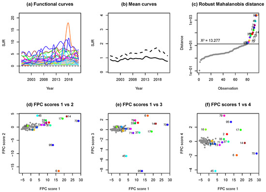
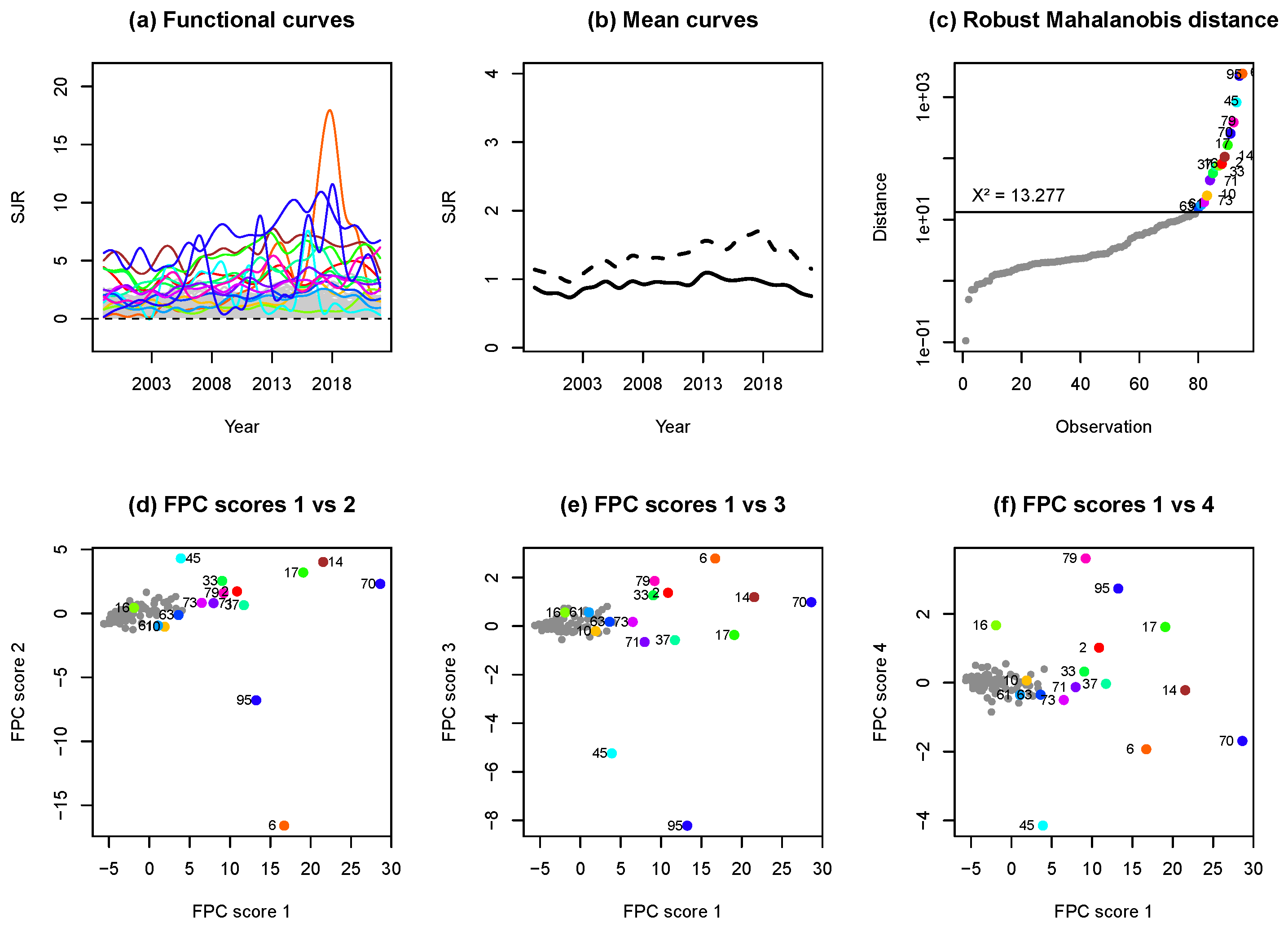
Figure 4a shows the functional curves corresponding to SJR data, the curves identified as outlier journals are presented in colors. Mean curves with outliers (dotted line) and without outliers (continuous line) are presented in Figure 4b. The robust MD for each journal relative to the cutoff is plotted in Figure 4c. Scatterplots of the first functional component versus the second, third and fourth functional components are shown in Figure 4d, Figure 4e, and Figure 4f, respectively.
Figure 4.
The visualization of SJR data for the Statistics and Probability category. (a) SJR functional curves, curves colored other than gray represent the outlier journal. (b) Mean curves with outliers (dotted line) and without outliers (continuous line). (c) The robust Mahalanobis distances of each journal and the cutoff. Biplots of functional principal components analysis: (d) FPC 1 vs. 2, (e) FPC 1 vs. 3 and (f) FPC 1 vs. 4.
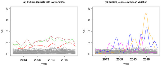
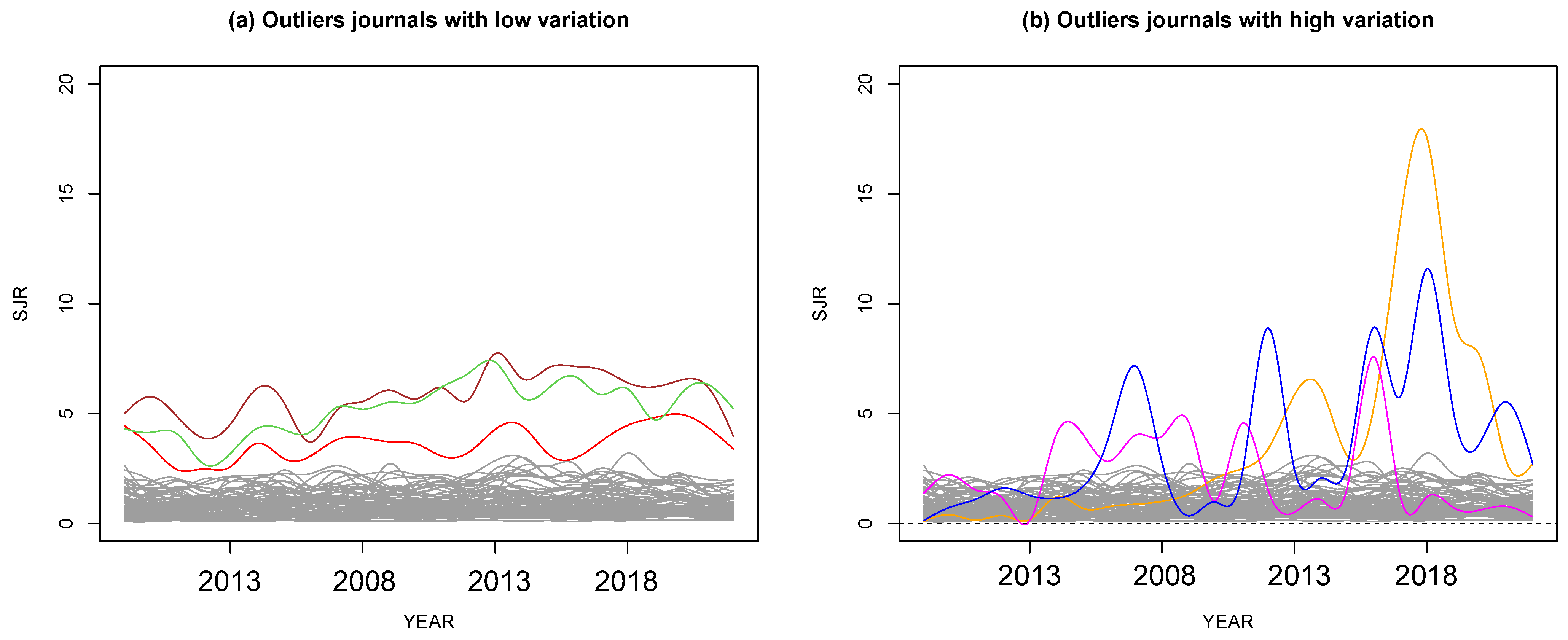
In the analysis of 16 outlier journals, they are categorized into two distinct groups based on their SJR trends over time (see Figure 5). The first group maintains consistently high SJR values above the functional mean across different years. This group includes Journal of the American Statistical Association, Journal of the Royal Statistical Society—Series B: Statistical Methodology, and Annals of Statistics. A second set of curves shows significant variability in their SJR values, characterized by years of pronounced growth and decline. For example, the Journal of Statistical Software has grown considerably since 2008, reaching a peak of 17.57 in 2018. Similarly, the journal Vital and Health Statistics—Series 1: Programs and Collection Procedures fluctuates between 0.12 and 7.59, with a maximum value in 2016. Meanwhile, Vital and Health Statistics—Series 2, Data Evaluation and Methods Research varies between 0.36 and 11.59, with its highest value in 2018. The observed patterns suggest different dynamics influencing their citation metrics; journals in group 1 benefit from established credibility and consistency in their fields, maintaining high SJR values. In contrast, group 2 journals may be more affected by specific trends, resulting in more significant year-to-year variability. In particular, some journals (e.g., Physical Review E) were flagged only by bagplot-based methods. This behavior can be explained by the fact that bagplot approaches emphasize centrality in the two-dimensional FPCA score space, whereas the robust Mahalanobis distance used in our approach evaluates deviations relative to the full covariance structure of the retained score vectors.
Figure 5.
Shift outlier (a) and isolated outlier (b) curves corresponding to journals from SJR data for the Statistics and Probability category. Curves colored other than gray represent the outlier journals.
6. Discussions
In Functional Data Analysis, outliers are defined as curves that exhibit behavior distinct from the dataset functions. This involves analyzing the discrete values as curves to identify anomalous observations that may not be evident at individual time points, but across their entire functional range. The proposed method for detecting functional outliers using the robust MCD estimator calculates robust Mahalanobis distance over the coefficient matrix of functional principal components. Given that the Mahalanobis distance follows a distribution with p degrees of freedom, observations with distances above the cutoff point are classified as outliers. The main contribution of this study is to detect functional outliers using the robust covariance matrix over functional principal components, in contrast to existing methods based on the first two principal components. When the method is applied to the El Niño SST dataset, it produces results identical to those of existing methods ISE [8], functional bagplot [7] and functional HDR boxplot [7]. When working with the SJR dataset, characterized by observations with significant fluctuations or drastic changes over time, the ISE method demonstrates similar results, with notable differences compared to functional HDR boxplot and functional bagplot methods.
For the El Niño SST dataset, from the scatterplots of the first two functional principal components (see Figure 3d), the four outlier temperatures reveal how they deviate from the non-atypical curves. The temperature for the year 1983 significantly deviates from the set of the FPC score 1 and FPC score 2 values, while the temperature for the year 1982 only shows a displacement in FPC score 2. This result is because the curve for the year 1983 significantly diverges from the group of temperatures from January to September (see Figure 3a). Conversely, the curve for the year 1952 only slightly deviates from the group of temperatures from October to December. These results influence the values of the robust MD, where the year 1983 has a distance of 59.03, exceeding the cutoff point of 13.277, while the curve for the year 1982 shows a distance of 24.47, close to the cutoff point (see Figure 3c).
In the analysis of the SJR dataset of a total of 95 journals, 16 are identified as outliers (see Table 9). The SJR curve of the Journal of Statistical Software, detected as an outlier by the four evaluated methods, deviates significantly from the group for the FPC score 1, FPC score 2, FPC score 3 and FPC score 4 values (see Figure 3). On the other hand, the Journal of Computational and Graphical Statistics, identified as an outlier only by the MCD 75 method, is positioned near to the point cloud of journals for the FPC score 2, FPC score 3, and FPC score 4 values, but it shows a deviation in the FPC score 1 values. Similarly, the American Statistician, detected as an outlier by the MCD 75 and ISE methods, approximates to the point cloud of journals for the FPC score 1, FPC score 2, and FPC score 3 values; however, it shows significant deviations in the FPC score 4 value. This is the main difference between our method and ISE, functional bagplot and functional HDR boxplot methods. The American Statistician shows no significant differences from the dataset when considering the first three functional components; however, the incorporation of the variability of the fourth functional component significantly influences the robust MD value. For the Journal of Statistical Software, the distance is 2420.98, significantly higher than the cutoff point of 13.28. In contrast, the curve of the American Statistician journal has a distance of 76.26. The Journal of Computational and Graphical Statistics has a distance of 15.66, which is close to the cutoff point.
In datasets that exhibit a relatively homogeneous structural configuration, the first principal components (usually the first two) tend to capture a substantial proportion of the total variance. However, when the data display drastic changes, multiple sources of variation, or complex structural patterns, the variance is more widely distributed across components. This implies the need to consider a larger number of principal components in order to achieve an adequate level of explained variance. As shown in Table A1–Table A6, it is observed that, on average, it is necessary to retain L principal components to accumulate more than 95% of the total variance. This behavior reflects the greater structural complexity of the dataset under analysis. In this context, the MCD 75 approach is adopted with the aim of working with the number of principal components required to capture the necessary variability under a robust criterion, thereby ensuring an adequate representation even in the presence of potential outliers or non-homogeneous structures.
All computations were conducted on an Apple M4 Pro processor with 12 cores and 25.8 GB of RAM. The computational times reported in Table 10 correspond to average runtimes over 100 simulation replicates per model. In each replicate, the dataset consists of 200 functional curves with a contamination rate of 20 percent. For the standard Mahalanobis approach, the total execution time is computed as the sum of the functional data preprocessing, FPCA decomposition, distance calculation, and outlier identification steps. Under this configuration, the total runtime remains highly stable across models, ranging from 0.065 to 0.070 s. For MCD 75, the total time is calculated analogously as the sum of functional data preprocessing, FPCA, robust distance computation, and outlier detection. Bagplot and ISE exhibit negligible computational cost, with average runtimes around 0.0013 to 0.0018 s and 0.0005 to 0.0006 s, respectively. In contrast, F-HDR presents the largest computational burden, requiring between 4.65 and 5.25 s per replicate.
Table 10.
Average execution times across models.
Author Contributions
Conceptualization, W.P.-R., A.G.L.-H. and M.E.; methodology, W.P.-R., A.G.L.-H. and M.E.; formal analysis, W.P.-R., A.G.L.-H. and M.E.; investigation, W.P.-R., A.G.L.-H. and M.E.; resources, W.P.-R., A.G.L.-H. and M.E.; writing—original draft preparation, W.P.-R., A.G.L.-H. and M.E.; writing—-review and editing, W.P.-R., A.G.L.-H. and M.E. All authors have read and agreed to the published version of the manuscript.
Funding
This research is partially supported by the project PID2023-149087NB-I00 financed by the Spanish Ministry of Science, Innovation and Universities (MICIU/AEI /10.13039/501100011033) also supported by the FEDER programme (FEDER, UE).
Data Availability Statement
The datasets and R code written to evaluate the method are available on GitHub: https://github.com/wilsonperezrc/rFDA (accessed on 22 May 2024).
Acknowledgments
Authors acknowledge the support of the IMAG-María de Maeztu grant CEX2020-001105-M/AEI/10.13039/501100011033, University of Granada.
Conflicts of Interest
The authors declare no conflicts of interest.
Abbreviations
The following abbreviations are used in this manuscript:
| FDA | Functional Data Analysis |
| PCA | Principal Component Analysis |
| FPCA | Functional Principal Component Analysis |
| MCD | Minimum Covariance Determinant |
| MD | Mahalanobis distance |
| HDR | Highest Density Region |
| SJR | SCImago Journal Rank |
| ISE | Integrated Squared Error |
Appendix A
Table A1.
Cumulative explained variance (CEV—second column), and the proportions of correctly () and falsely () detected outliers for each method and with each number of functional principal components in Model 1.
Figure A1.
Proportions of correctly () and falsely () detected outliers for each method and with each number of functional principal components. Red vertical lines indicate the 95% and 99% levels of explained variability. (a) Correctly identified outliers (), (b) falsely identified outliers () over the six models.
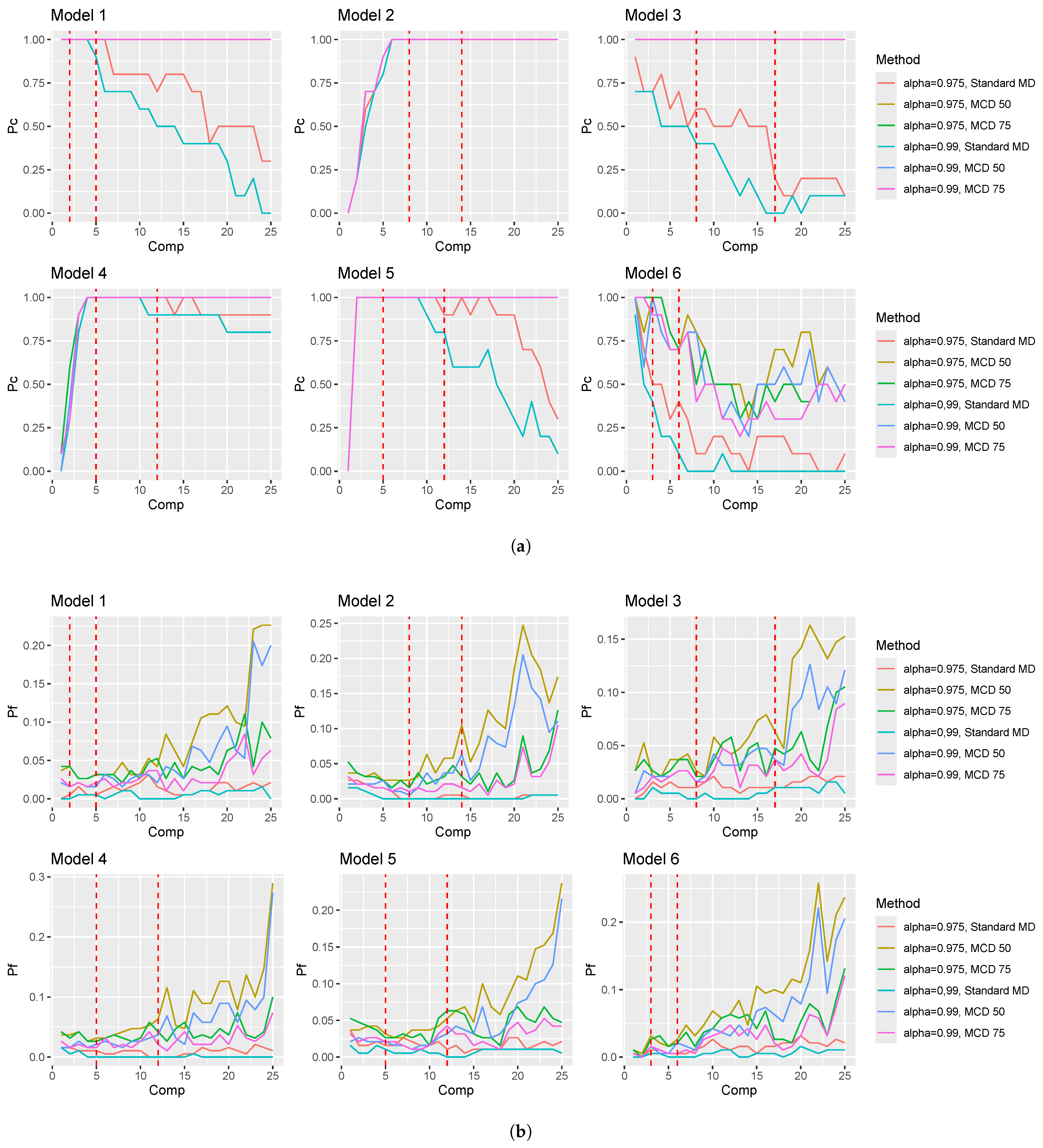
Table A2.
Cumulative explained variance (CEV—second column), and the proportions of correctly () and falsely () detected outliers for each method and with each number of functional principal components in Model 2.
Table A3.
Cumulative explained variance (CEV—second column), and the proportions of correctly () and falsely () detected outliers for each method and with each number of functional principal components in Model 3.
Table A4.
Cumulative explained variance (CEV—second column), and the proportions of correctly () and falsely () detected outliers for each method and with each number of functional principal components in Model 4.
Table A5.
Cumulative explained variance (CEV—second column), and the proportions of correctly () and falsely () detected outliers for each method and with each number of functional principal components in Model 5.
Table A6.
Cumulative explained variance (CEV—second column), and the proportions of correctly () and falsely () detected outliers for each method and with each number of functional principal components in Model 6.
References
- Ramsay, J.O.; Silverman, B.W. Functional Data Analysis; Springer Series in Statistics; Springer: New York, NY, USA, 2005. [Google Scholar]
- Febrero, M.; Galeano, P.; González-Manteiga, W. Outlier detection in functional data by depth measures, with application to identify abnormal NOx levels. Environmetrics 2007, 4, 331–345. [Google Scholar] [CrossRef] [Scilit]
- Fraiman, R.; Muniz, G. Trimmed means for functional data. Test 2001, 2, 419–440. [Google Scholar] [CrossRef] [Scilit]
- Cuevas, A.; Febrero, M.; Fraiman, R. On the use of the bootstrap for estimating functions with functional data. Comput. Stat. Data Anal. 2006, 2, 1063–1074. [Google Scholar] [CrossRef] [Scilit]
- Sun, Y.; Genton, M.G. Functional Boxplots. J. Comput. Graph. Stat. 2011, 2, 316–334. [Google Scholar] [CrossRef] [Scilit]
- López-Pintado, S.; Romo, J. On the Concept of Depth for Functional Data. J. Am. Stat. Assoc. 2009, 104, 718–734. [Google Scholar] [CrossRef] [Scilit]
- Hyndman, R.J.; Shang, H.L. Rainbow Plots, Bagplots, and Boxplots for Functional Data. J. Comput. Graph. Stat. 2010, 1, 29–45. [Google Scholar] [CrossRef] [Scilit]
- Hyndman, R.J.; Ullah, M.S. Robust forecasting of mortality and fertility rates: A functional data approach. Comput. Stat. Data Anal. 2007, 10, 4942–4956. [Google Scholar] [CrossRef] [Scilit]
- Arribas-Gil, A.; Romo, J. Shape outlier detection and visualization for functional data: The outliergram. Biostatistics 2014, 4, 603–619. [Google Scholar] [CrossRef] [Scilit] [PubMed]
- Rousseeuw, P.J.; Raymaekers, J.; Hubert, M. A Measure of Directional Outlyingness with Applications to Image Data and Video. J. Comput. Graph. Stat. 2018, 4, 345–359. [Google Scholar] [CrossRef] [Scilit]
- Dai, W.; Genton, M.G. Multivariate Functional Data Visualization and Outlier Detection. J. Comput. Graph. Stat. 2018, 4, 923–934. [Google Scholar] [CrossRef] [Scilit]
- Rousseeuw, P.J.; van Zomeren, B.C. Unmasking Multivariate Outliers and Leverage Points. J. Am. Stat. Assoc. 1990, 85, 633–639. [Google Scholar] [CrossRef]
- Rocke, D.M.; Woodruff, D.L. Identification of Outliers in Multivariate Data. J. Am. Stat. Assoc. 1996, 91, 1047–1061. [Google Scholar] [CrossRef]
- Rousseeuw, P.J.; van Driessen, K. A Fast Algorithm for the Minimum Covariance Determinant Estimator. Technometrics 1999, 3, 212. [Google Scholar] [CrossRef]
- Rousseeuw, P.J. Multivariate Estimation with High Breakdown Point. In Mathematical Statistics and Applications; Springer: Dordrecht, The Netherlands, 1985. [Google Scholar]
- Leys, C.; Klein, O.; Dominicy, Y.; Ley, C. Detecting multivariate outliers: Use a robust variant of the Mahalanobis distance. J. Exp. Soc. Psychol. 2018, 74, 150–156. [Google Scholar] [CrossRef] [Scilit]
- Sawant, P.; Billor, N.; Shin, H. Functional outlier detection with robust functional principal component analysis. Comput. Stat. 2011, 1, 83–102. [Google Scholar] [CrossRef] [Scilit]
- Oguamalam, J.; Radojičić, U.; Filzmoser, P. Minimum regularized covariance trace estimator and outlier detection for functional data. Technometrics 2024, 66, 588–599. [Google Scholar] [CrossRef] [Scilit]
- Abdi, H.; Williams, L.J. Principal component analysis. Wiley Interdiscip. Rev. Comput. Stat. 2010, 4, 433–459. [Google Scholar] [CrossRef] [Scilit]
- Tukey, J.W. Exploratory Data Analysis; Springer Series in Statistics; Pearson: New York, NY, USA, 1977. [Google Scholar]
- Rousseeuw, P.J.; Ruts, I.; Tukey, J.W. The Bagplot: A Bivariate Boxplot. Am. Stat. 1999, 4, 382–387. [Google Scholar] [CrossRef] [Scilit]
- Croux, C.; Filzmoser, P.; Oliveira, M.R. Algorithms for projection–pursuit robust principal component analysis. Chemom. Intell. Lab. Syst. 2007, 2, 218–225. [Google Scholar] [CrossRef] [Scilit]
- Tukey, J.W. Mathematics and the Picturing of Data; Canadian Mathematical Congress: Vancouver, BC, Canada, 1975. [Google Scholar]
- Rosenblatt, M. Remarks on Some Nonparametric Estimates of a Density Function. Ann. Math. Stat. 1956, 3, 832–837. [Google Scholar] [CrossRef] [Scilit]
- Hubert, M.; Rousseeuw, P.J.; Verboven, S. A fast method for robust principal components with applications to chemometrics. Chemom. Intell. Lab. Syst. 2002, 1, 101–111. [Google Scholar] [CrossRef] [Scilit]
- Mahalanobis, P.C. On the generalized distance in statistics. Proc. Natl. Inst. Sci. India 1936, 2, 49–55. [Google Scholar]
- De Maesschalck, R.; Jouan-Rimbaud, D.; Massart, D.L. The Mahalanobis distance. Chemom. Intell. Lab. Syst. 2000, 1, 1–18. [Google Scholar] [CrossRef] [Scilit]
- Johnson, R.A.; Wichern, D.W. Applied Multivariate Statistical Analysis; Prentice Hall: Upper Saddle River, NJ, USA, 1998. [Google Scholar]
- Rousseeuw, P.J.; van Zomeren, B.C. Robust Distances: Simulations and Cutoff Values. In The IMA Volumes in Mathematics and Its Applications; Springer: New York, NY, USA, 1991. [Google Scholar]
- Croux, C.; Haesbroeck, G. Influence function and efficiency of the minimum covariance determinant scatter matrix estimator. J. Multivar. Anal. 1999, 2, 161–190. [Google Scholar] [CrossRef] [Scilit]
- Pison, G.; Rousseeuw, P.J.; Filzmoser, P.; Croux, C. Robust factor analysis. J. Multivar. Anal. 2003, 1, 145–172. [Google Scholar] [CrossRef] [Scilit]
- Hubert, M.; Rousseeuw, P.J.; Van Aelst, S. High-Breakdown Robust Multivariate Methods. Stat. Sci. 2008, 23, 92–119. [Google Scholar] [CrossRef] [Scilit]
- Rousseeuw, P.J. Least median of squares regression. J. Am. Stat. Assoc. 1984, 79, 871–880. [Google Scholar] [CrossRef]
- Maronna, R.A.; Martin, R.D.; Yohai, V.J. Robust Statistics Theory and Methods; John Wiley & Sons: Hoboken, NJ, USA; Wiley: Chichester, UK, 2006. [Google Scholar]
- Hubert, M.; Rousseeuw, P.J.; Verboven, T. A deterministic algorithm for robust location and scatter. J. Comput. Graph. Stat. 2012, 21, 618–637. [Google Scholar] [CrossRef] [Scilit]
- Anderson, T.W. An Introduction to Multivariate Statistical Analysis; John Wiley & Sons, Inc.: Hoboken, NJ, USA; Wiley-Interscience: New York, NY, USA, 2003. [Google Scholar]
- Hardin, J.; Rocke, D.M. The distribution of robust distances. J. Comput. Graph. Stat. 2005, 14, 928–946. [Google Scholar] [CrossRef] [Scilit]
- Rousseeuw, P.J.; Hubert, M. Anomaly detection by robust statistics. Wiley Interdiscip. Rev. Data Min. Knowl. Discov. 2018, 8, e1236. [Google Scholar] [CrossRef] [Scilit]
- Hubert, M.; Rousseeuw, P.J.; Segaert, P. Multivariate functional outlier detection. Stat. Methods Appl. 2015, 24, 177–202. [Google Scholar] [CrossRef] [Scilit]
- Dioses, T.; Dávalos, R.; Zuzunaga, J. Niño 1982–1983 and 1997–1998: Effects on Peruvian Jack Mackerel and Peruvian Chub Mackere. Investig. Mar. 2002, 1, 103–104. [Google Scholar] [CrossRef] [Scilit]

Disclaimer/Publisher’s Note: The statements, opinions and data contained in all publications are solely those of the individual author(s) and contributor(s) and not of MDPI and/or the editor(s). MDPI and/or the editor(s) disclaim responsibility for any injury to people or property resulting from any ideas, methods, instructions or products referred to in the content. |
© 2026 by the authors. Licensee MDPI, Basel, Switzerland. This article is an open access article distributed under the terms and conditions of the Creative Commons Attribution (CC BY) license.