On Unit J-Shaped Distributions: Properties and Estimation with Applications

Abstract

This study is a detailed study of unit J-shaped distributions which establishes and examines the unit Topp–Leone distribution. The proposed study presents a mathematically tractable model of bounded data with strong skewness and boundary effects. Various basic distributional properties, such as moments, entropy measures, order statistics, and L-moments, are obtained in explicit form, which provides a full analytic description of the model. Type-II censoring is applied to develop some statistical inferential methods. The usefulness of the suggested distribution is illustrated by the application to the normalized water use efficiency indicators and censored survival time data. The findings are useful to the theory of unit distributions, as they introduce new analytics that have been demonstrated to be beneficial in practice and demonstrate that the theory is effective in applications with limited and censored data.

1. Introduction

Probability distributions that take values on the unit interval (0, 1) take centre stage in describing proportions, rates, reliability indices and lifetime data that are limited. Traditional ones are the beta, Kumaraswamy, and unit Weibull distributions, which have been widely applied because of their versatility and analytical ease. Nonetheless, most bounded data sets have a strong J-shaped or reversed J-shaped character, in which the conventional models might fail to give a reasonable fit.

The Topp–Leone distribution that was introduced by Topp and Leone [1] is a significant family of J-shaped distributions with a functional form and a bathtub-shaped hazard rate. Although it has attractive features, initial investigations were aimed at low-order moments and simple reliability features. Nadarajah and Kotz [2] made a significant contribution in this direction, deriving explicit expressions of moments, central moments, and characteristic functions in terms of hypergeometric functions.

Recently, there has been a renewed interest in unit distributions due to their use in economics, actuarial science, and environmental research. When classical lifetime distributions are transformed to the unit interval, it is common to have a model with increased interpretability and a higher likelihood of fitting the data within a limited range. In this context, a natural model (which has restricted support to (0, 1)) is the unit Topp–Leone distribution (UTLD), which produces a one-parameter model that is parsimonious and has strong skewness at the boundaries.

The UTLD provides a mathematically treatable model of dealing with bathtub-shaped data. It offers a lightweight but elastic single-parameter model and explicit closed-form expressions of major distributional properties that are useful for making statistical inferences. The UTLD has practical applicability, which is identified in the paper by the application to normalized water use efficiency indicators (WUIs) and censored survival data, and it works well in reproducing the boundary behavior and skewness of these data sets.

This paper is an attempt at offering a thorough treatment of the statistical properties of the UTLD. In this context, it adds to the growing body of literature on unit distributions that are defined on the interval (0, 1) that are popularly used to model proportions (e.g., Afuecheta et al. [3], Mazucheli et al. [4], and Stojanović et al. [5]). In this framework, the UTLD provides a clean and analytically manageable alternative, especially when they are required to model strongly J-shaped bounded data with a high degree of inferential simplicity and practical applicability. On the basis of the previous findings on J-shaped distributions, we obtain moments, entropy measures, order statistics, and L-moments in closed form. In addition, we find estimation under type-II censoring with maximum likelihood and Bayesian methods, both with the aid of simulation and real-data studies.

The rest of the paper will be structured in the following manner. Section 2 presents the UTLD and comments on its key distributional features. In Section 3, some of the statistical properties of the proposed model are obtained, which incorporate moments, entropy measures, order statistics, and L-moments. Section 4 is devoted to statistical inference in Type-II censoring, in which the classical and Bayesian estimations are developed and evaluated in a simulation study. Section 4 also introduces the applications to real data sets to explain how the model can be applied practically. Lastly, Section 5 sums up the paper and contains a summary of the key findings and future research directions.

2. Unit Topp–Leone Distribution

In Section 2, the development of a distribution, defined by the unit interval (0, 1), and its basic properties are obtained. The developed distribution is the so-called UTLD. The cumulative distribution function, probability density function, and hazard rate function are explicitly expressed, and the key characteristics of these functions are discussed.

The cumulative distribution function (CDF), $F\left(x\right)$ UTLD can be presented as follows:

$$F\left(x\right)=x^{\alpha }{(2-x)}^{\alpha },0\le x\le 1\mathrm{and}0<\alpha <1.$$

(1)

This definition arises by applying the transform $Y=\frac{X}{b};0\le x\le b<\infty$ to the CDF of the Topp–Leone distribution; see Nadarajah and Kotz [2].

Alternatively, the Topp–Leone family of distributions presented by Al-Shomrani et al. [6] offers the mechanism of generators in the following form:

$$F\left(x\right)={\left[G\left(x\right)\right]}^{\alpha }{\left[2-G\left(x\right)\right]}^{\alpha }.$$

(2)

In which G(x) is an arbitrary baseline distribution. Al-Shomrani et al. [6] mainly study the structural properties of the family, series expansions, hazard rate representation and estimation of parameters in cases of complete data, using the Topp–Leone Exponential model. The current work has different scopes and objectives. Instead of analyzing the general Topp–Leone generator, we give a detailed analytic and inferential treatment of the unit-bounded formulation that we get when the baseline distribution is uniform on (0, 1). Specifically, we obtain explicit closed-form results on entropy measures, L-moments, and order statistics, and formulate statistical inference in Type-II censoring in both classical and Bayesian settings. These properties and censoring-based inference procedures have not been elaborated on in the case of the unit formulation of the Topp–Leone construction.

The corresponding probability density function (PDF), $f\left(x\right)$ is given by:

$$f\left(x\right)=2\alpha x^{\alpha -1}{(2-x)}^{\alpha -1}(1-x),0\le x\le 1\mathrm{and}0<\alpha <1.$$

(3)

One can see that $f\left(x\right)>0,$ and ${\int }_0^{1}f\left(x\right)dx=1$ by assuming that $t=x(x-1)$ which leads to

$\frac{dt}{dx}=2(1-x)$ and $0<t<1.$

In case of $\alpha =1;$ the UTLD reduces to the Beta distribution, $B(v,w)$ with the parameters $v=1$ and $w=2.$

The hazard rate function $h\left(x\right)$ can be formulated as follows:

$$h\left(x\right)={\displaystyle \frac{2\alpha x^{\alpha -1}{(2-x)}^{\alpha -1}(1-x)}{1-x^{\alpha }{(2-x)}^{\alpha }}}.$$

(4)

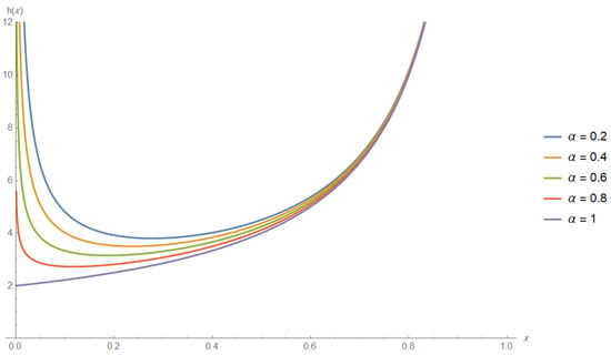
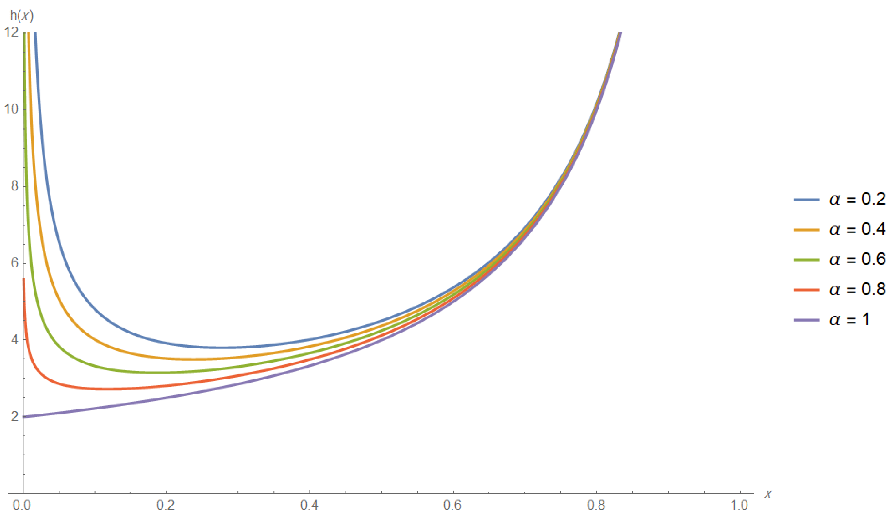
The hazard rate function of the proposed model is plotted in Figure 1 to show the hazard rate of some values of the shape parameter $\alpha$. The curves show the typical behavior of J-shaped ones, where the curvature is greatly altered by the shape parameter. Specifically, the hazard function is J-shaped in its distribution on the unit interval, whereby it declines and rises. The behavior substantiates the classification of this model to the family of J-shaped distributions and the ability of the model to be appropriate in the modelling of reliability data with early- and late-life effects.

Figure 1. Hazard function of the UTLD for different values of $\alpha$.

The UTLD can arise from the Topp–Leone Distribution (TLP) by letting the parameter $b=1$ in Equation (1) defined by Nadarajah and Kotz [2]. Therefore, the following properties, discussed by Nadarajah and Kotz [2], can be derived:

• r-th Moment, $E\left[X^r\right]=r>0.$

  $$E\left[X^r\right]=2^{r+2\alpha }\alpha \left[\begin{array}{c}Be\left(\begin{array}{c}r+\alpha ,\alpha ;{\displaystyle \frac{1}{2}}\end{array}\right)-2Be\left(\begin{array}{c}1+r+\alpha ,\alpha ;{\displaystyle \frac{1}{2}}\end{array}\right)\end{array}\right],$$

  (5)

where $Be(a,b;u)={\int }_0^u{x}^{a-1}{(1-x)}^{b-1}dx,$ is the incomplete beta function.

• Central moments

$$\begin{array}{cc}\hfill {\mu }_2& ={\displaystyle \frac{1}{\alpha +1}}-{16}^{\alpha }{\displaystyle \frac{{\Gamma }^4(\alpha +1)}{{\Gamma }^2(2\alpha +2)}},\hfill \\ \hfill {\mu }_3& =3{\left(2\right)}^{1+2\alpha }(\alpha +2){\displaystyle \frac{{\Gamma }^2(\alpha +1)}{\Gamma (2\alpha +4)}}-4^{2+3\nu }{(\alpha +1)}^3{\displaystyle \frac{{\Gamma }^6(\alpha +1)}{{\Gamma }^3(2\alpha +3)}},\hfill \\ \hfill {\mu }_4& ={\displaystyle \frac{2}{{(\alpha +1)}^2}}+3{\left(2\right)}^{3+4\alpha }(\alpha +1)(2\alpha +3){\displaystyle \frac{{\Gamma }^4(\alpha +1)}{{\Gamma }^2(2\alpha +4)}}-3{\left(16\right)}^{1+2\alpha }{(1+\alpha )}^4{\displaystyle \frac{{\Gamma }^8(\alpha +1)}{{\Gamma }^4(2\alpha +3)}}.\hfill \end{array}$$

The skewness (S) and kurtosis (K) measures can be computed as follows:

$$S={\displaystyle \frac{{\mu }_3}{{\mu }_2^{3/2}}},\mathrm{and}K={\displaystyle \frac{{\mu }_4}{{\mu }_2^2}},$$

(6)

• Characteristic function

  $$\mathbb{E}\left[e^{itX}\right]={\displaystyle \frac{2^{\alpha }}{1+\alpha }}{\Phi }_1\left(\alpha ,1-\alpha ;2;\frac{1}{2},-it\right),$$

  (7)

  where ${\Phi }_1(·)$ denotes the confluent hypergeometric function of two variables, defined by

  $${\Phi }_1(\omega ,\delta ;\gamma ;u,v)=\sum _{k,l=0}^{\infty }{\displaystyle \frac{{\left(\omega \right)}_{k+l}{\left(\delta \right)}_k}{{\left(\gamma \right)}_{k+l}}}{\displaystyle \frac{u^k{v}^l}{k!l!}},$$

  (8)

and ${\left(\omega \right)}_k=\omega (1+\omega )\dots (k-1+\omega ).$ For more details about Equation (8), see Gradshteyn and Ryzhik [7], p. 1005, Equation (9).

3. Statistical Properties of Unit Topp–Leone Distribution

Once the probability density and the distribution functions of the UTLD are defined, this section formulates some important distributional properties, such as order statistics, some entropy measures, and L-moments, that are newly developed in this paper for the UTLD. These properties are necessary to comprehend the shape, variability, and inferential behavior of the model.

3.1. Order Statistics

Order statistics are central to reliability theory and the analysis of censored data because they provide a natural model for analyzing failure times, extremities, and incomplete observations. Order statistic approaches are a popular technique in the fields of survival analysis, models of reliability, and inference under censoring plans; see Balakrishnan and Cramer [8]; Kundu and Raqab [9]. In the case of the unit Topp–Leone distribution, it is possible to explicitly obtain the density and the moments of order statistics by replacing the cumulative distribution and density functions in the general order-statistic expression. Analytically tractable solutions are obtained by taking advantage of binomial expansions and the beta function identities to get closed-form expressions of the expected values of the minimum and maximum order statistics.

Let $X_{\left(k\right)}$ denote the kth order statistic, $k=1,\dots ,n$. The density function of $X_{\left(k\right)}$ is

$$f_{X_{\left(k\right)}}\left(x\right)={\displaystyle \frac{n!}{(k-1)!(n-k)!}}{\left[F\left(x\right)\right]}^{k-1}{[1-F\left(x\right)]}^{n-k}f\left(x\right),0<x<1.$$

Substituting the expressions for $F\left(x\right)$ and $f\left(x\right)$, from (1) and (3), respectively, we obtain,

$$f_{X_{\left(k\right)}}\left(x\right)={\displaystyle \frac{n!}{(k-1)!(n-k)!}}2\alpha (1-x){\left[x(2-x)\right]}^{\alpha k-1}{\left[1-{\left(x(2-x)\right)}^{\alpha }\right]}^{n-k}.$$

The expected value of the kth order statistic is

$$\mathbb{E}\left[X_{\left(k\right)}\right]={\int }_0^{1}x{f}_{X_{\left(k\right)}}\left(x\right)dx.$$

Using the binomial expansion

$${\left[1-{\left(x(2-x)\right)}^{\alpha }\right]}^{n-k}=\sum _{j=0}^{n-k}{(-1)}^j\left({\displaystyle \genfrac{}{}{0pt}{}{n-k}{j}}\right){\left[x(2-x)\right]}^{\alpha j},$$

we obtain

$$\mathbb{E}\left[X_{\left(k\right)}\right]={\displaystyle \frac{n!}{(k-1)!(n-k)!}}2\alpha \sum _{j=0}^{n-k}{(-1)}^j\left({\displaystyle \genfrac{}{}{0pt}{}{n-k}{j}}\right){\int }_0^{1}x(1-x){\left[x(2-x)\right]}^{\alpha (k+j)-1}dx.$$

(9)

For a closed form, $\mathbb{E}\left[X_{\left(k\right)}\right],$ the following lemma needs to be proved.

Lemma 1.

For any $\beta >0$,

$${\int }_0^{1}x(1-x){\left[x(2-x)\right]}^{\beta -1}dx={\displaystyle \frac{1}{2}}\left[{\displaystyle \frac{1}{\beta }}-B\left(\beta ,{\displaystyle \frac{3}{2}}\right)\right],$$

where $B(·,·)$ denotes the Beta function.

Applying Lemma 1, with $\beta =\alpha (k+j)$ in (9), we obtain,

$$\mathbb{E}\left[X_{\left(k\right)}\right]={\displaystyle \frac{n!}{(k-1)!(n-k)!}}\alpha \sum _{j=0}^{n-k}{(-1)}^j\left({\displaystyle \genfrac{}{}{0pt}{}{n-k}{j}}\right)\left[{\displaystyle \frac{1}{\alpha (k+j)}}-B\left(\alpha (k+j),{\displaystyle \frac{3}{2}}\right)\right].$$

(10)

Special Cases

Minimum order statistic, $X_{\left(1\right)}$:

$$\mathbb{E}\left[X_{\left(1\right)}\right]=n\alpha \sum _{j=0}^{n-1}{(-1)}^j\left({\displaystyle \genfrac{}{}{0pt}{}{n-1}{j}}\right)\left[{\displaystyle \frac{1}{\alpha (1+j)}}-B\left(\alpha (1+j),{\displaystyle \frac{3}{2}}\right)\right].$$

Maximum order statistic, $X_{\left(n\right)}$:

$$\mathbb{E}\left[X_{\left(n\right)}\right]=\alpha \left[{\displaystyle \frac{1}{\alpha n}}-B\left(\alpha n,{\displaystyle \frac{3}{2}}\right)\right].$$

Mean, $n=1$:

$$\mathbb{E}\left[X\right]=\alpha \left[{\displaystyle \frac{1}{\alpha }}-B\left(\alpha ,{\displaystyle \frac{3}{2}}\right)\right].$$

3.2. Entropy Measures

Entropy measures quantify the uncertainty and information content related to a random variable. Entropy is an important concept in signal processing, reliability, and information theory of bounded distributions; for more details, see Cover and Thomas [10]. Both Shannon and Rényi entropies are considered for the UTLD, and explicit forms are obtained with respect to both the Beta and Digamma functions. These findings indicate the influence of the shape parameter on the uncertainty structure of the distribution.

3.2.1. Shannon Entropy

The Shannon entropy of a continuous random variable with density f is defined by

$$H\left(X\right)=-{\int }_0^{1}f\left(x\right)logf\left(x\right)dx.$$

Using the decomposition

$$logf\left(x\right)=log\left(2\alpha \right)+log(1-x)+(\alpha -1)log\left[x\right(2-x\left)\right],$$

we obtain

$$\begin{array}{cc}\hfill H\left(X\right)& =-log\left(2\alpha \right){\int }_0^{1}f\left(x\right)dx-{\int }_0^{1}f\left(x\right)log(1-x)dx\hfill \\ & -(\alpha -1){\int }_0^{1}f\left(x\right)log\left[x(2-x)\right]dx.\hfill \end{array}$$

Since ${\int }_0^{1}f\left(x\right)dx=1$, it follows that

$$H\left(X\right)=-log\left(2\alpha \right)-I_1-(\alpha -1)I_2,$$

where

$$I_1={\int }_0^{1}f\left(x\right)log(1-x)dx,I_2={\int }_0^{1}f\left(x\right)log\left[x(2-x)\right]dx.$$

$$I_1=2\alpha {\int }_0^1(1-x){\left[x(2-x)\right]}^{\alpha -1}log(1-x)dx={\displaystyle \frac{\alpha }{2}}{\int }_0^1{t}^{\alpha -1}log(1-t)dt.$$

Using the identity

$${\int }_0^1{t}^{\alpha -1}log(1-t)dt={\displaystyle \frac{1}{\alpha }}\left[\psi \left(1\right)-\psi (\alpha +1)\right],0<\alpha <1,$$

where $\psi (·)$ denotes the Digamma function, we obtain

$$I_1={\displaystyle \frac{1}{2}}\left[\psi \left(1\right)-\psi (\alpha +1)\right]=-{\displaystyle \frac{1}{2}}\left[\gamma +\psi (\alpha +1)\right],$$

with $\gamma$ denoting Euler’s constant, c.f. Andrews et al. [11]. Similarly,

$$I_2=2\alpha {\int }_0^1(1-x){\left[x(2-x)\right]}^{\alpha -1}log\left[x(2-x)\right]dx.$$

Let

$$t=x(2-x)=1-{(1-x)}^2,dt=2(1-x)dx.$$

Then

$$I_2=\alpha {\int }_0^1{t}^{\alpha -1}logtdt=-{\displaystyle \frac{1}{\alpha }}.$$

Substituting $I_1$ and $I_2$, the Shannon entropy reduces to

$$\begin{array}{|c|}\hline H\left(X\right)=-log\left(2\alpha \right)+{\displaystyle \frac{1}{2}}\left[\psi (\alpha +1)+\gamma \right]+1-{\displaystyle \frac{1}{\alpha }}.\\ \hline\end{array}$$

3.2.2. Rényi Entropy

For $q>0$, $q\ne 1$, the Rényi entropy of order q is defined by

$$H_q^{\left(R\right)}\left(X\right)={\displaystyle \frac{1}{1-q}}log\left({\int }_0^{1}f{\left(x\right)}^{q}dx\right).$$

Raising the density to the power q,

$$f{\left(x\right)}^q={\left(2\alpha \right)}^q{(1-x)}^q{\left[x(2-x)\right]}^{q(\alpha -1)}.$$

Using the transformation $t=x(2-x)$, we obtain

$$\begin{array}{cc}\hfill {\int }_0^{1}f{\left(x\right)}^{q}dx& =2^{q-1}{\alpha }^q{\int }_0^1{t}^{q(\alpha -1)}{(1-t)}^{(q-1)/2}dt\hfill \\ & =2^{q-1}{\alpha }^{q}B\left(q(\alpha -1)+1,{\displaystyle \frac{q+1}{2}}\right).\hfill \end{array}$$

Thus, the Rényi entropy is

$$\begin{array}{|c|}\hline H_q^{\left(R\right)}\left(X\right)={\displaystyle \frac{1}{1-q}}log\left[2^{q-1}{\alpha }^{q}B\left(q(\alpha -1)+1,{\displaystyle \frac{q+1}{2}}\right)\right].\\ \hline\end{array}$$

It is noticed that measures of entropy of the UTLD are determined by the shape parameter $\alpha$, which is in control of the extent of uncertainty and dispersion. Both Shannon and Rényi entropies are represented in closed form using beta and digamma functions, giving an analytically tractable form. In addition, the Rényi entropy approaches the Shannon entropy as $q⟶1$, which is an assurance of the internal consistency of the entropy framework.

3.3. L-Moments

Linear combinations of order statistics, also known as L-moments, are known to be strong alternatives to standard moments, particularly when the data are skewed and heavy-tailed. They are of particular interest to probability-weighted moments (PWMs), which offer a useful and efficient derivation and estimation methodology in terms of the distribution function. Researchers like Hosking [12] have pointed out that L-moments obtained using PWMs are less sensitive to outliers and sampling variability, and they provide accurate measurements of location, variability, skewness, and kurtosis. The above properties explain the application of the probability-weighted moments in this paper to obtain the L-moments of the UTLD.

The population L-moments ${\lambda }_r$ may be defined through the quantile representation

$${\lambda }_r={\int }_0^{1}Q\left(u\right)P_{r-1}\left(u\right)du,r\ge 1,$$

where $Q\left(u\right)=F^{-1}\left(u\right)$ denotes the quantile function and $P_{r-1}\left(u\right)$ is the shifted Legendre polynomial of degree $r-1$.

The shifted Legendre polynomials admit the expansion

$$P_{r-1}\left(u\right)=\sum _{j=0}^{r-1}{c}_{r-1,j}{u}^j,$$

where

$$c_{r-1,j}={(-1)}^{r-1-j}\left({\displaystyle \genfrac{}{}{0pt}{}{r-1}{j}}\right)\left({\displaystyle \genfrac{}{}{0pt}{}{r+j-1}{j}}\right),j=0,1,\dots ,r-1.$$

The quantile function of the UTLD is obtained by solving

$$u={\left[x(2-x)\right]}^{\alpha }.$$

The solution in $(0,1)$ is

$$Q\left(u\right)=1-\sqrt{1-u^{1/\alpha }},0<u<1.$$

(11)

Reduction to PWMs and substituting the polynomial expansion of $P_{r-1}\left(u\right)$ into the definition of ${\lambda }_r$ yields

$${\lambda }_r=\sum _{j=0}^{r-1}{c}_{r-1,j}{\int }_0^{1}Q\left(u\right)u^{j}du,$$

where the PWMs are defined as follows:

$${\beta }_j={\int }_0^{1}Q\left(u\right)u^{j}du=\mathbb{E}\left[XF{\left(X\right)}^j\right],j=0,1,2,\dots$$

so that

$${\lambda }_r=\sum _{j=0}^{r-1}{c}_{r-1,j}{\beta }_j.$$

Using the explicit form $Q\left(u\right)$ defined in (11), then

$${\beta }_j={\int }_0^1\left(1-\sqrt{1-u^{1/\alpha }}\right)u^{j}du.$$

Splitting the integral, we obtain

$${\beta }_j={\int }_0^1{u}^{j}du-{\int }_0^1{u}^j\sqrt{1-u^{1/\alpha }}du.$$

The first integral equals ${(j+1)}^{-1}$. For the second, let $w=u^{1/\alpha }$, so that $u=w^{\alpha }$ and $du=\alpha w^{\alpha -1}dw$. Then

$${\int }_0^1{u}^j\sqrt{1-u^{1/\alpha }}du=\alpha {\int }_0^1{w}^{\alpha j+\alpha -1}{(1-w)}^{1/2}dw=\alpha B\left(\alpha (j+1),{\displaystyle \frac{3}{2}}\right),$$

hence,

$${\beta }_j={\displaystyle \frac{1}{j+1}}-\alpha B\left(\alpha (j+1),{\displaystyle \frac{3}{2}}\right),j=0,1,2,\dots$$

Substituting the above expression for ${\beta }_j$ into the expansion of ${\lambda }_r$ yields the general formula

$$\begin{array}{|c|}\hline {\lambda }_r={\displaystyle \sum _{j=0}^{r-1}}{(-1)}^{r-1-j}\left({\displaystyle \genfrac{}{}{0pt}{}{r-1}{j}}\right)\left({\displaystyle \genfrac{}{}{0pt}{}{r+j-1}{j}}\right)\left[{\displaystyle \frac{1}{j+1}}-\alpha B\left(\alpha (j+1),{\displaystyle \frac{3}{2}}\right)\right],r\ge 1.\\ \hline\end{array}$$

(12)

3.3.1. Derivation of the First Four L-Moments

Since the rth L-moment of the UTLD is given by

$${\lambda }_r=\sum _{j=0}^{r-1}{c}_{r-1,j}\left[{\displaystyle \frac{1}{j+1}}-\alpha B\left(\alpha (j+1),{\displaystyle \frac{3}{2}}\right)\right],r\ge 1,$$

for convenience, define

$$A_j={\displaystyle \frac{1}{j+1}}-\alpha B\left(\alpha (j+1),{\displaystyle \frac{3}{2}}\right),j=0,1,2,3.$$

(13)

First L-moment: For $r=1$, we have $c_{0,0}=1$, and therefore

$${\lambda }_1=A_0=1-\alpha B\left(\alpha ,{\displaystyle \frac{3}{2}}\right).$$

Second L-moment: For $r=2$, the coefficients are

$$c_{1,0}=-1,c_{1,1}=2.$$

Hence

$$\begin{array}{cc}\hfill {\lambda }_2& =-A_0+2A_1\hfill \\ & =-\left(1-\alpha B\left(\alpha ,{\displaystyle \frac{3}{2}}\right)\right)+2\left({\displaystyle \frac{1}{2}}-\alpha B\left(2\alpha ,{\displaystyle \frac{3}{2}}\right)\right)\hfill \\ & =\alpha \left[B\left(\alpha ,{\displaystyle \frac{3}{2}}\right)-2B\left(2\alpha ,{\displaystyle \frac{3}{2}}\right)\right].\hfill \end{array}$$

Third L-moment: For $r=3$, the coefficients are

$$c_{2,0}=1,c_{2,1}=-6,c_{2,2}=6.$$

Thus

$$\begin{array}{cc}\hfill {\lambda }_3& =A_0-6A_1+6A_2\hfill \\ & =\left(1-\alpha B\left(\alpha ,{\displaystyle \frac{3}{2}}\right)\right)-6\left({\displaystyle \frac{1}{2}}-\alpha B\left(2\alpha ,{\displaystyle \frac{3}{2}}\right)\right)+6\left({\displaystyle \frac{1}{3}}-\alpha B\left(3\alpha ,{\displaystyle \frac{3}{2}}\right)\right)\hfill \\ & =\alpha \left[6B\left(2\alpha ,{\displaystyle \frac{3}{2}}\right)-6B\left(3\alpha ,{\displaystyle \frac{3}{2}}\right)-B\left(\alpha ,{\displaystyle \frac{3}{2}}\right)\right].\hfill \end{array}$$

Fourth L-moment: For $r=4$, the coefficients are

$$c_{3,0}=-1,c_{3,1}=12,c_{3,2}=-30,c_{3,3}=20.$$

Hence,

$$\begin{array}{cc}\hfill {\lambda }_4& =-A_0+12A_1-30A_2+20A_3\hfill \\ & =-\left(1-\alpha B\left(\alpha ,{\displaystyle \frac{3}{2}}\right)\right)+12\left({\displaystyle \frac{1}{2}}-\alpha B\left(2\alpha ,{\displaystyle \frac{3}{2}}\right)\right)\hfill \\ & -30\left({\displaystyle \frac{1}{3}}-\alpha B\left(3\alpha ,{\displaystyle \frac{3}{2}}\right)\right)+20\left({\displaystyle \frac{1}{4}}-\alpha B\left(4\alpha ,{\displaystyle \frac{3}{2}}\right)\right)\hfill \\ & =\alpha \left[B\left(\alpha ,{\displaystyle \frac{3}{2}}\right)-12B\left(2\alpha ,{\displaystyle \frac{3}{2}}\right)+30B\left(3\alpha ,{\displaystyle \frac{3}{2}}\right)-20B\left(4\alpha ,{\displaystyle \frac{3}{2}}\right)\right].\hfill \end{array}$$

Now, the first four L-moments of the UTLD can be summarized as follows:

$${\lambda }_1=1-\alpha B\left(\alpha ,{\displaystyle \frac{3}{2}}\right),$$

$${\lambda }_2=\alpha \left[B\left(\alpha ,{\displaystyle \frac{3}{2}}\right)-2B\left(2\alpha ,{\displaystyle \frac{3}{2}}\right)\right],$$

$${\lambda }_3=\alpha \left[6B\left(2\alpha ,{\displaystyle \frac{3}{2}}\right)-6B\left(3\alpha ,{\displaystyle \frac{3}{2}}\right)-B\left(\alpha ,{\displaystyle \frac{3}{2}}\right)\right],$$

$${\lambda }_4=\alpha \left[B\left(\alpha ,{\displaystyle \frac{3}{2}}\right)-12B\left(2\alpha ,{\displaystyle \frac{3}{2}}\right)+30B\left(3\alpha ,{\displaystyle \frac{3}{2}}\right)-20B\left(4\alpha ,{\displaystyle \frac{3}{2}}\right)\right].$$

L-Coefficient of Variation

The L-coefficient of variation (L-CV) is defined as:

$$\tau ={\displaystyle \frac{{\lambda }_2}{{\lambda }_1}}.$$

For the UTLD, substituting the expressions for ${\lambda }_1$ and ${\lambda }_2$ yields,

$$\begin{array}{|c|}\hline \tau ={\displaystyle \frac{\alpha \left[B\left(\alpha ,\frac{3}{2}\right)-2B\left(2\alpha ,\frac{3}{2}\right)\right]}{1-\alpha B\left(\alpha ,\frac{3}{2}\right)}}.\\ \hline\end{array}$$

L-Skewness

The L-skewness measure is defined by

$${\tau }_3={\displaystyle \frac{{\lambda }_3}{{\lambda }_2}}.$$

Using the expressions for ${\lambda }_2$ and ${\lambda }_3$, the common factor $\alpha$ cancels, giving

$$\begin{array}{|c|}\hline {\tau }_3={\displaystyle \frac{6B\left(2\alpha ,\frac{3}{2}\right)-6B\left(3\alpha ,\frac{3}{2}\right)-B\left(\alpha ,\frac{3}{2}\right)}{B\left(\alpha ,\frac{3}{2}\right)-2B\left(2\alpha ,\frac{3}{2}\right)}}.\\ \hline\end{array}$$

L-Kurtosis

The L-kurtosis measure is defined by

$${\tau }_4={\displaystyle \frac{{\lambda }_4}{{\lambda }_2}}.$$

Substituting the expressions for ${\lambda }_4$ and ${\lambda }_2$ yields

$$\begin{array}{|c|}\hline {\tau }_4={\displaystyle \frac{B\left(\alpha ,\frac{3}{2}\right)-12B\left(2\alpha ,\frac{3}{2}\right)+30B\left(3\alpha ,\frac{3}{2}\right)-20B\left(4\alpha ,\frac{3}{2}\right)}{B\left(\alpha ,\frac{3}{2}\right)-2B\left(2\alpha ,\frac{3}{2}\right)}}.\\ \hline\end{array}$$

3.3.2. Gamma-Function Representation

Using the identity

$$B\left(a,{\displaystyle \frac{3}{2}}\right)={\displaystyle \frac{\sqrt{\pi }}{2}}{\displaystyle \frac{\Gamma \left(a\right)}{\Gamma \left(a+\frac{3}{2}\right)}},$$

define

$$R_m\left(\alpha \right)={\displaystyle \frac{\Gamma \left(m\alpha \right)}{\Gamma \left(m\alpha +\frac{3}{2}\right)}}.$$

(14)

Then, the L-moment ratios may equivalently be written as:

$$\tau ={\displaystyle \frac{\frac{\alpha \sqrt{\pi }}{2}\left[R_1\left(\alpha \right)-2R_2\left(\alpha \right)\right]}{1-\frac{\alpha \sqrt{\pi }}{2}{R}_1\left(\alpha \right)}},$$

$${\tau }_3={\displaystyle \frac{6R_2\left(\alpha \right)-6R_3\left(\alpha \right)-R_1\left(\alpha \right)}{R_1\left(\alpha \right)-2R_2\left(\alpha \right)}},{\tau }_4={\displaystyle \frac{R_1\left(\alpha \right)-12R_2\left(\alpha \right)+30R_3\left(\alpha \right)-20R_4\left(\alpha \right)}{R_1\left(\alpha \right)-2R_2\left(\alpha \right)}}.$$

The L-moment framework gives a full and strong description of the proposed distribution. All population L-moments and their ratios are clearly defined in terms of the shape parameter, making sure that both interpretation and analysis are easy. Having all L-moments and simplifying them to closed forms for certain values shows that the model is flexible and useful for describing skewed bounded data.

4. Statistical Inference

Statistical inference for the parameter of UTLD is developed under type-II censoring, a common scheme in reliability and life-testing experiments; see Balakrishnan and Aggarwala [13]. The likelihood function is presented by combining contributions from censored observations and the UTLD as follows:

$$L\left(\alpha \right|data)={\displaystyle \frac{{\left(2\alpha \right)}^{r}n!}{\left(n-r\right)!}}\prod _{i=1}^r\left[\begin{array}{c}{x}_i^{\alpha -1}{(2-x_i)}^{\alpha -1}(1-x_i)\end{array}\right]{\left[\begin{array}{c}1-x_r^{\alpha }{(2-x_r)}^{\alpha }\end{array}\right]}^{n-r},$$

(15)

where n denotes the total sample size, and r is the number of observed failures under the Type-II censoring scheme. The log-likelihood function and its partial derivative with respect to the parameter $\alpha$ are presented, respectively, as follows:

$$\begin{array}{ccc}\hfill lnL\left(\alpha \right|data)& =& rln\left(2\alpha \right)+ln(n!)-ln((n-r)!)+(n-r)ln\left[\begin{array}{c}1-x_r^{\alpha }{(2-x_r)}^{\alpha }\end{array}\right]+\hfill \\ & & \sum _{i=1}^r\left[\begin{array}{c}\left(\alpha -1\right)ln{x}_i+\left(\alpha -1\right)ln(2-x_i)+ln(1-x_i)\end{array}\right],\hfill \end{array}$$

(16)

$$\begin{array}{ccc}\hfill {\displaystyle \frac{\partial lnL\left(\alpha \right|data)}{\partial \alpha }}& =& {\displaystyle \frac{r}{\alpha }}+\sum _{i=1}^r\left[\begin{array}{c}ln{x}_i+ln(2-x_i)\end{array}\right]+\hfill \\ & & {\displaystyle \frac{(r-n)\left[\begin{array}{c}{x}_r^{\alpha }{(2-x_r)}^{\alpha }ln(2-x_r)+x_r^{\alpha }{(2-x_r)}^{\alpha }ln{x}_r\end{array}\right]}{\left[\begin{array}{c}1-x_r^{\alpha }{(2-x_r)}^{\alpha }\end{array}\right]}}.\hfill \end{array}$$

(17)

By letting Equation (17) equal zero to get the Maximum Likelihood Estimate (MLE) of $\alpha ,$ it is noted that a numerical algorithm, like Newton–Raphson, should be applied for estimating $\alpha .$ The applied steps of the Newton–Raphson algorithm are described in detail by Al-Moisheer et al. [14]. The $\left(1-\chi \right)100\%$ approximate confidence intervals (ACIs) for the parameter $\alpha$ can be written as

$$({\widehat{\alpha }}_L,{\widehat{\alpha }}_U)=\widehat{\alpha }\pm z_{1-{\displaystyle \frac{\chi }{2}}}\sqrt{var\left(\widehat{\alpha }\right)},$$

where $z_{1-\frac{\zeta }{2}}$ is the percentile of the standard normal distribution with left-tail probability $1-\frac{\chi }{2}$ and $var\left(\widehat{\alpha }\right)$ represent the asymptotic variances of maximum likelihood estimates, which can be calculated using the inverse of the Fisher information matrix. The asymptotic variance–covariance matrix for the maximum likelihood estimates can be formulated as follows:

$$I^{-1}\left(\alpha \right)={\left[-\left({\displaystyle \frac{{\partial }^{2}lnL}{{\partial }^2\alpha }}\right)\right]}_{\downarrow \alpha =\widehat{\alpha }}^{-1},$$

(18)

where

$${\displaystyle \frac{{\partial }^{2}lnL\left(\alpha \right|data)}{\partial {\alpha }^2}}={\displaystyle \frac{{\left[\begin{array}{c}\left(2-x_r\right)x_r\end{array}\right]}^{\alpha }\left(6-{\alpha }^2(n-3){\left(ln(2-x_r)+ln\left(x_r\right)\right)}^2\right)-3\left[\begin{array}{c}{\left[\left(2-x_r\right)x_r\right]}^{2\alpha }+1\end{array}\right]}{{\left[\begin{array}{c}{\left[\left(2-x_r\right)x_r\right]}^{\alpha }-1\end{array}\right]}^2}},$$

for more details see Cohen [15].

Since the parameter space of the UTLD is restricted to $0<\alpha <1$, the numerical maximization of the log-likelihood in Equation (16) may, in some situations (especially under heavy censoring), produce estimates that fall outside the admissible interval. To guarantee the parameter admissibility and improve numerical stability, we consider an inverse logit transformation as follows:

Let

$$\alpha ={\displaystyle \frac{1}{1+e^{-\theta }}},\theta \in \mathbb{R},$$

for more details about the logit transformation, see Seiffert et al. [16]. Maximization of the likelihood with respect to $\theta$ automatically ensures that the resulting estimate satisfies $0<\alpha <1$. By the invariance property of maximum likelihood estimates, if $\widehat{\theta }$ is the MLE of $\theta$, then

$$\widehat{\alpha }={\displaystyle \frac{1}{1+e^{-\widehat{\theta }}}}$$

is the corresponding MLE of $\alpha$.

Since the asymptotic variance of $\widehat{\alpha }$ is obtained from the inverse Fisher information in Equation (18), the delta method, see Casella and Berger [17] may be used to obtain the variance of the transformed estimate. Noting that

$${\displaystyle \frac{d\alpha }{d\theta }}=\alpha (1-\alpha ),$$

we obtain

$$\mathrm{Var}\left(\widehat{\alpha }\right)\approx {\widehat{\alpha }}^2{(1-\widehat{\alpha })}^2{I}^{-1}\left(\widehat{\theta }\right).$$

where $I^{-1}\left(\widehat{\theta }\right)$ denotes the inverse observed Fisher information evaluated at the MLE of the parameter $\theta$.

Consequently, an approximate $(1-\chi )100\%$ confidence interval for $\alpha$ can be written as follows:

$$\widehat{\alpha }\pm z_{1-\chi /2}\sqrt{{\widehat{\alpha }}^2{(1-\widehat{\alpha })}^2{I}^{-1}\left(\widehat{\theta }\right)}.$$

To account for prior information and asymmetric loss structures, Bayesian inference is also considered. Assuming a beta prior distribution for the parameter $\alpha$, as follows:

$$\pi (\alpha ;a,b)={\displaystyle \frac{1}{Beta(a,b)}}{\alpha }^{a-1}{(1-\alpha )}^{b-1}.$$

(19)

Upon using the likelihood function defined in Equation (15) and the beta prior distribution, the posterior distribution ${\pi }^{\ast }\left(\alpha \right|data)$ can be formulated as follows:

$${\pi }^{\ast }\left(\alpha \right|data){\alpha }^{r+a-1}{(1-\alpha )}^{b-1}\prod _{i=1}^r\left[\begin{array}{c}{x}_i^{\alpha -1}{(2-x_i)}^{\alpha -1}\end{array}\right]{\left[\begin{array}{c}1-x_r^{\alpha }{(2-x_r)}^{\alpha }\end{array}\right]}^{n-r}.$$

(20)

Bayesian estimates are obtained under squared error (SEL) and LINEX loss functions, allowing flexibility in penalizing over- or under-estimation. However, obtaining Bayesian estimates for the parameter $\alpha$ under certain loss functions usually requires evaluating the ratio of complicated integrals; see Al-Moisheer et al. [18]. Therefore, evaluating these complicated integrals requires applying the Markov Chain Monte Carlo (MCMC) approach and getting the Bayesian point estimates for $\alpha .$ The credible interval (CR) can be computed upon sorting the replicated point estimates of $\alpha$ at confidence level (CL) $\left(1-\chi \right)100\%.$ The following steps (Algorithm 1) illustrate the MCMC approach based on “Metropolis–Hastings” algorithm:

Algorithm 1 MCMC Approach Based on “Metropolis–Hastings” Algorithm

1. Start with $,{\alpha }^{\left(o\right)}$

2. Put $j=1$

3. Generate ${\alpha }^{\left(j\right)}$ with normal suggested distribution $N({\alpha }^{\left(j-1\right)},Var\left(\alpha \right))$, where $Var\left(\alpha \right)$ can be obtained from the asymptotic variances of the maximum likelihood estimate, which can be calculated using the inverse of the Fisher information matrix.

(i) Generate a proposal ${\alpha }^{\ast }$ from $N({\alpha }^{\left(j-1\right)},Var\left(\alpha \right)),$

(ii) Evaluate the acceptance probabilities $${\rho }_{\alpha }=min\left[1,{\displaystyle \frac{{\pi }^{\ast }\left({\alpha }^{\ast }\right|data)}{{\pi }^{\ast }\left({\alpha }^{\left(j-1\right)}\right|data)}}\right],$$

4. Compute ${\alpha }^{\left(j\right)}.$

5. Put $j=j+1$

6. Repeat Steps (3–5) N times.

7. To guarantee the convergence and to remove the influence of the selection of initial values, the first M simulated varieties are ignored. Then, the selected samples are ${\alpha }^{\left(j\right)},j=M+1,\dots ,N,$ for sufficiently large N, forms an approximate posterior sample that can be used to obtain the Bayes MCMC point estimates ${\alpha }^{\left(j\right)}$ based on the SEL function as follows: $${\widehat{\alpha }}_{MCMC-SEL}={\displaystyle \frac{1}{N-M}}\sum _{j=M+1}^{N-M}{\alpha }^{\left(j\right)},$$ while the Bayesian estimate of $\alpha$ under the LINEX Loss function can be formulated as follows: $${\widehat{\alpha }}_{MCMC-LINEX}={\displaystyle \frac{-1}{C}}ln\left[\begin{array}{c}\frac{1}{N-M}{\displaystyle \sum _{j=M+1}^{N-M}}{e}^{-C{\alpha }^{\left(j\right)}}\end{array}\right],C\ne 0.$$

8. To compute the credible intervals of $\alpha$, sort ${\alpha }^{\left(i\right)},$$i=M+1,...,N$. Then the $100(1-\gamma )\%$ credible intervals of $\alpha$ is given by $$\left[\begin{array}{ccc}{\alpha }_{\left(N\gamma /2\right)}& ,& {\alpha }_{\left(N\left(1-\gamma /2\right)\right)}\end{array}\right].$$

Moreover, the MCMC algorithm was implemented by using Wolfram Mathematica, version 12, via a defined statistical package called “Metropolis–Hastings”; details are available via the following URL: https://resources.wolframcloud.com/FunctionRepository/resources/MetropolisHastingsSequence/, accessed on 3 January 2026.

4.1. Simulation Study

A Monte Carlo simulation study is conducted to assess the finite-sample performance of the proposed estimators. The bias and mean squared error (MSE) are reported for different sample sizes and censoring schemes, where 1000 replicated samples are generated from the UTLD based on the inverse transformation method. For the MCMC approach, the Metropolis–Hastings algorithm was applied based on 10,000 chains with 2000 burned chains at the beginning of the process to improve the obtained results. Regarding the Beta prior, its hyperparameters are chosen to be $B(a,b)=B(0.01,0.01).$ The obtained confidence intervals were compared with Average Length of the Confidence Interval (ALCI) and coverage probability (CP). Trace plots and posterior stability diagnostics were used to assess MCMC convergence. The Metropolis–Hastings algorithm showed approximately a 70 percent acceptance rate (30 percent rejection rate) so that mixing is sufficient and the posterior inferences are sound.

The results in Table 1 indicate that bias and MSE decrease with an increase in the sample size and establish the consistency of all estimators in Type-II censoring.

Table 1. Bias and MSE values of the parameter $\alpha$ at ${\alpha }_0=0.6$.

		$\mathrm{MLE}$		$\mathrm{SEL}$		$\mathrm{LINEX}$
						$\mathit{c}=-\mathbf{2}$		$\mathit{c}=\mathbf{2}$
$\mathit{n}$	$\mathit{r}$	Bias	MSE	Bias	MSE	Bias	MSE	Bias	MSE
30	20	0.0680	0.0047	0.0874	0.0292	0.1030	0.0325	0.0719	0.0261
40	20	0.0611	0.0038	0.0656	0.0211	0.0781	0.0235	0.0533	0.0190
50	30	0.0527	0.0029	0.0466	0.0156	0.0563	0.0172	0.0372	0.0142
60	50	0.0427	0.0019	0.0324	0.0117	0.0401	0.0128	0.0250	0.0108

As observed in Table 2, the confidence interval based on MLE has full coverage but is wider. In comparison, Bayesian credible intervals are shorter and more informative, and the coverage probabilities get better as the size of the sample gets larger.

Table 2. ALCIs and CPs for the parameter $\alpha$ at ${\alpha }_0=0.6$.

		$\mathrm{ACI}$				$\mathrm{CRI}$
		$\mathbf{90}\%$		$\mathbf{95}\%$		$\mathbf{90}\%$		$\mathbf{95}\%$
$\mathit{n}$	$\mathit{r}$	ALCI	CP	ALCI	CP	ALCI	CP	ALCI	CP
30	20	0.3683	1.0000	0.7103	1.0000	0.3851	0.8010	0.4438	0.8600
40	20	0.3339	1.0000	0.6576	1.0000	0.3516	0.8350	0.4076	0.8850
50	30	0.2932	1.0000	0.5952	1.0000	0.3095	0.8400	0.3616	0.8970
60	50	0.2560	1.0000	0.5370	1.0000	0.2766	0.8450	0.3263	0.9010

On the whole, both the classical and Bayesian methods are effective, and Bayesian tools are more accurate in the context of intervals in censored cases.

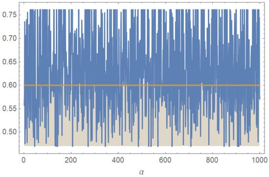
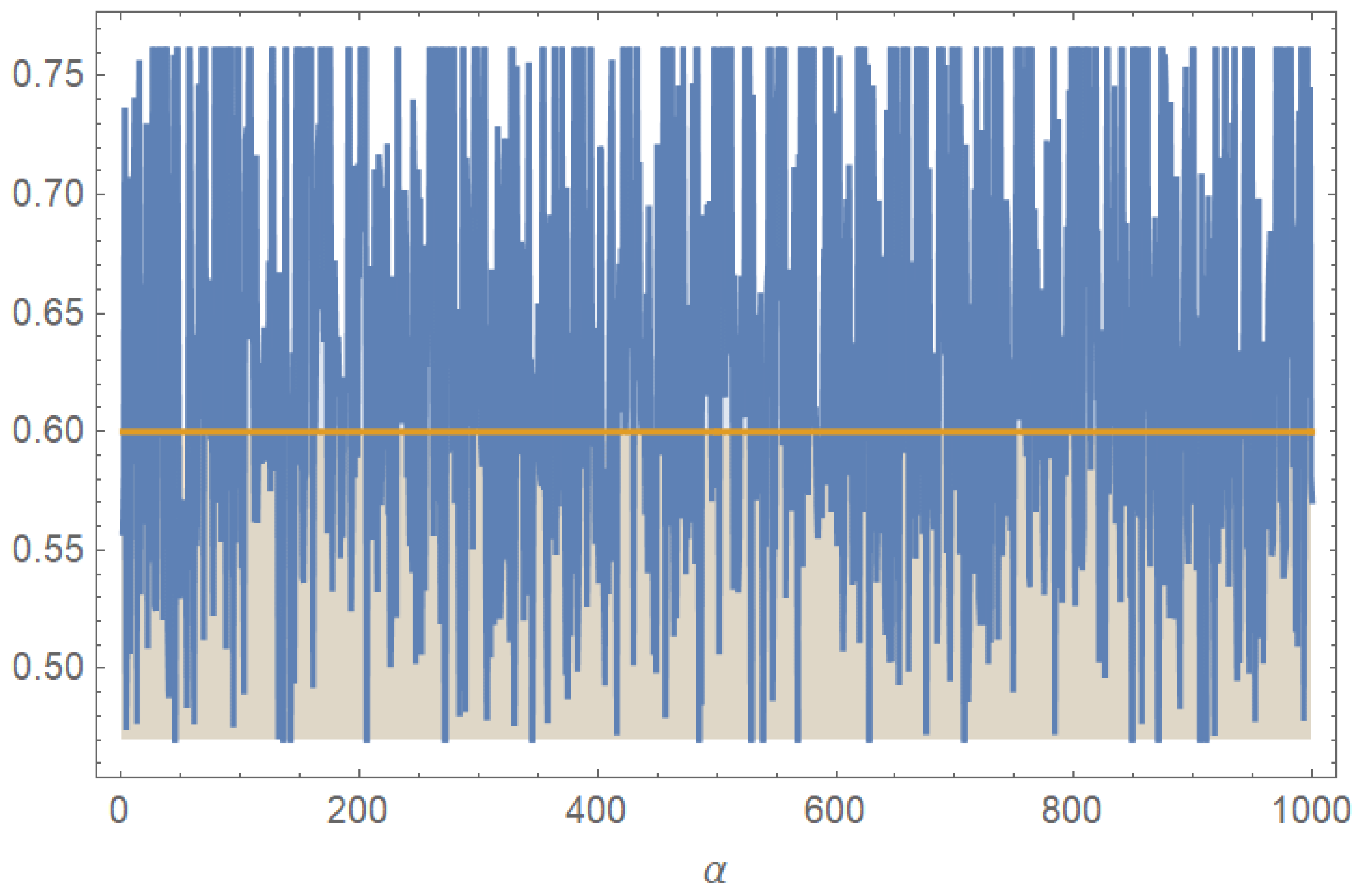
The traces of the Bayesian estimates of the parameter $\alpha$ are shown in Figure 2 as a result of the MCMC procedure, where the yellow line in Figure 2 refers to the true value of the parameter $\alpha$ that was used to generate the simulated samples. The mixing of the plots is good, and the behavior of the plots is quite stable in the course of the iterations, and no clear tendencies or sudden shifts are observed, which indicates that the Markov chains have approached their stationary distribution. This implies that the Bayesian estimation algorithm is sound and the obtained posterior samples are a reasonable source of inference on the parameter of the model.

Figure 2. Tracing plots of the parameter $\alpha$.

4.2. Applications and Data Analysis

It is shown in this subsection that the suggested UTLD is applicable to real data. The analysis mentions the possibility of the model fitting both the limited and the censored data; inference is handled in both the classical and Bayesian models, and the model adequacy is evaluated through some goodness-of-fit measures.

4.2.1. Analysis of Water Use Efficiency Indicator for Services

The analysis uses annual data on the water use efficiency indicator for services (WUIS) for Saudi Arabia, originally compiled for the period 2000–2020 from the Food and Agriculture Organization of the United Nations (FAO) SDG 6.4.1 database and reported as economic value added per cubic meter of water withdrawn (US$/m³). The original data are also available and were recently referred to by Elzaki and Al-Mahish [19]. To ensure comparability and to meet the distributional requirements of the UTLD, the original series was normalized to the unit interval (0, 1). Observations at the boundaries (0 and 1) were excluded, and the empirical analysis focuses on the 2001–2014 sub-period, which is treated as a right-censored Type-II sample. This selected interval represents a relatively stable phase of gradual improvements in service-sector water use efficiency, prior to the pronounced post-2014 increases observed in the full 2000–2020 dataset, which are likely driven by structural reforms, technological progress, and policy shifts in water management.

Normalized Censored Values of WUIS
$0.12219$	$0.11751$	$0.24438$	$0.33621$	$0.18159$	$0.1577$	$0.13488$
$0.01667$	$0.44962$	$0.34538$	$0.22905$	$0.3159$	$0.3562$	$0.44588$

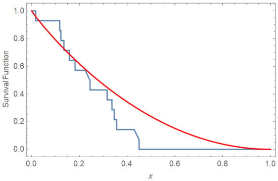
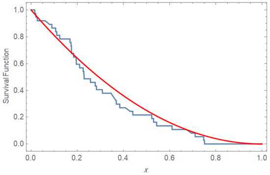
The Kolmogorov–Smirnov (K-S) test is applied to show how the UTLD is a well-fitted model to the normalized censored values of WUIS, as displayed in Figure 3. The computed value of the K-S test is $0.287606$ with a p-value equal to $0.161323$.

Figure 3. K-S test for WUIS censored data.

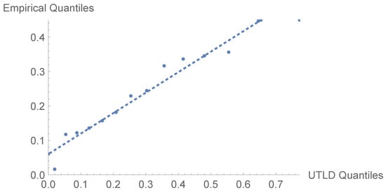
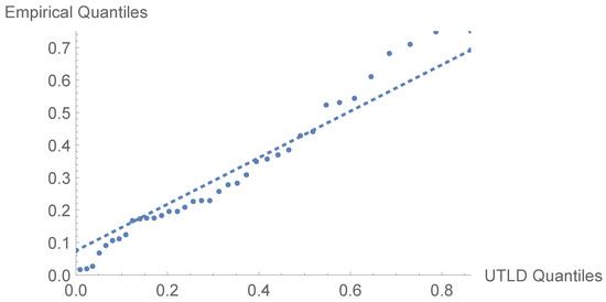
Figure 4 demonstrates the Q-Q plot of the empirical quantiles of the normalized censored UWUIS data and theoretical quantiles of the UTLD. The plot points are not far from the straight line of reference, where the deviations are small at the upper tail. This is an indication of a good fit between the empirical distribution and the fitted Unit Topp–Leone model, which confirms the suitability of the Unit Topp–Leone to model the WUIS bounded and censored data. After sorting the values of WUIS and applying the developed inference approaches presented earlier in Section 4 by setting $n=19$ and $r=14$, we summarize the obtained results in Table 3.

Figure 4. Q-Q plot for WUIS censored data.

Table 3. Extrapolated results from censored data.

Point Estimates of $\alpha$				Interval Estimates of $\alpha$
MLE	Bayesian SEL	Bayesian-LINEX Loss		CL	ACI	CRI
		$c_1=-2$	$c_2=2$	$90\%$	$0.620157,0.919589$	$0.816518,0.993298$
$0.76987$	$0.95787$	$0.96016$	$0.95524$	$95\%$	$0.619059,0.920687$	$0.793581,0.993298$

Table 3 shows that the UTLD is useful in explaining the censored data of water use efficiency. There is some stability in the estimated values of the shape parameter in all the methods, which indicates that the findings are not influenced by the inference method of choice. Bayesian estimates are more consistent, and the associated credible intervals are much smaller than the asymptotic ones, which give more accurate and useful inference. Applied-wise, the findings facilitate the application of the proposed model to analyzing efficiency indicators that are limited and censored.

4.2.2. Analysis of Survival Times

The dataset consists of survival times (in years) for 43 patients diagnosed with a specific type of leukaemia, originally reported by Laha [20]. Each observation represents the length of time a patient survived following diagnosis. The data are positive, continuous, and exhibit a right-skewed pattern, which is typical of survival data in medical studies. Such datasets are commonly analyzed using lifetime and survival analysis models, where censoring mechanisms may arise due to loss to follow-up or study termination. The ordered nature and variability of the survival times make this dataset suitable for illustrating parametric lifetime distributions and inferential methods in reliability and biomedical statistics. The data are sorted and normalized to be in the range (0, 1), and outlier values are omitted. Therefore, n is adjusted to be $41,$ and r is selected to be $37.$

Normalized Censored Values of Survival Times
$0.016$	$0.0204$	$0.0268$	$0.068$	$0.09$	$0.1063$	$0.1112$
$0.124$	$0.1686$	$0.1732$	$0.1751$	$0.1751$	$0.1842$	$0.195$
$0.1959$	$0.2099$	$0.2254$	$0.2286$	$0.2295$	$0.257$	$0.2778$
$0.283$	$0.3085$	$0.3492$	$0.357$	$0.3689$	$0.3841$	$0.4277$
$0.4404$	$0.5224$	$0.5304$	$0.5435$	$0.6104$	$0.6814$	$0.7103$
$0.7475$	$0.751$

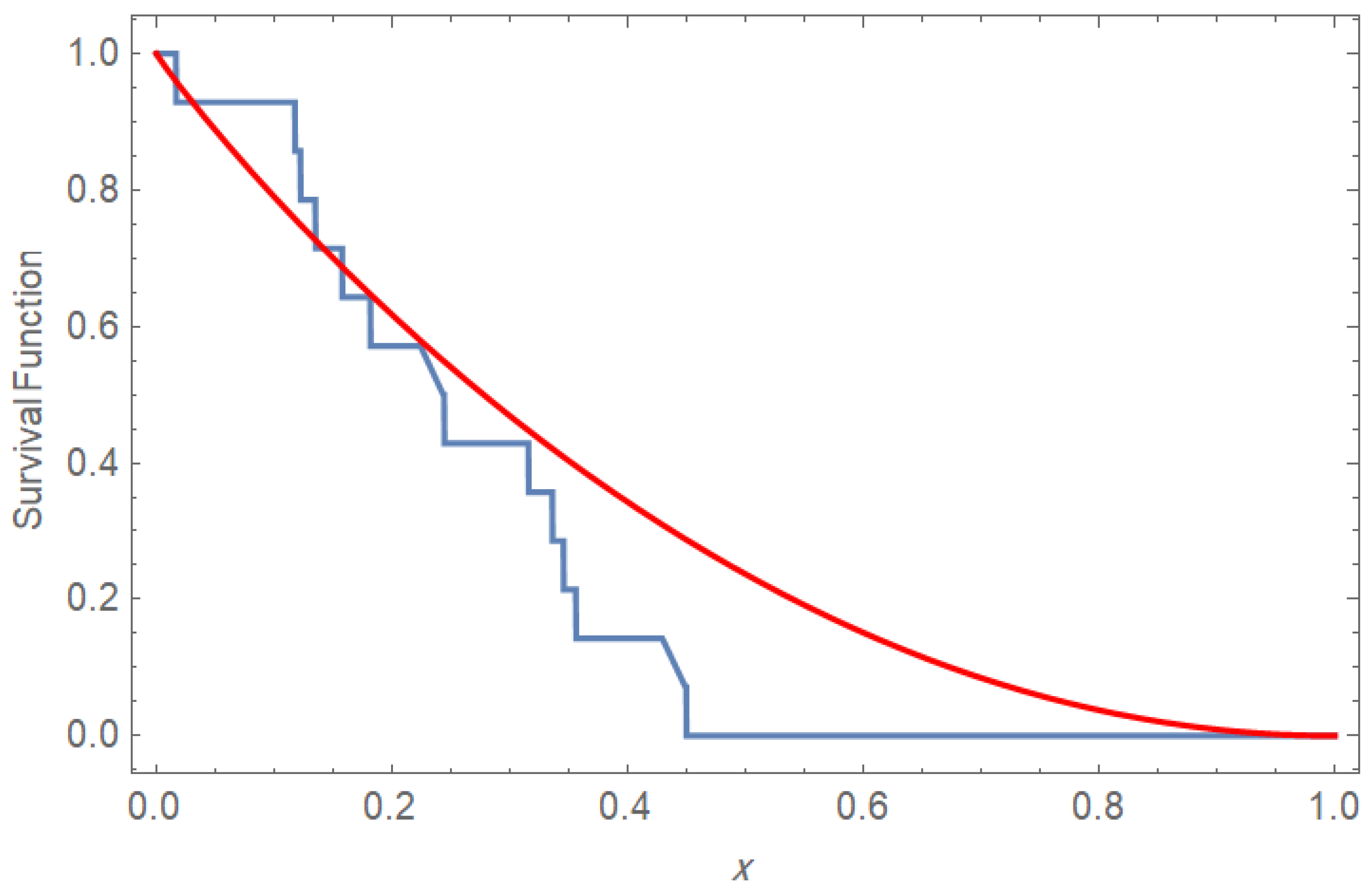
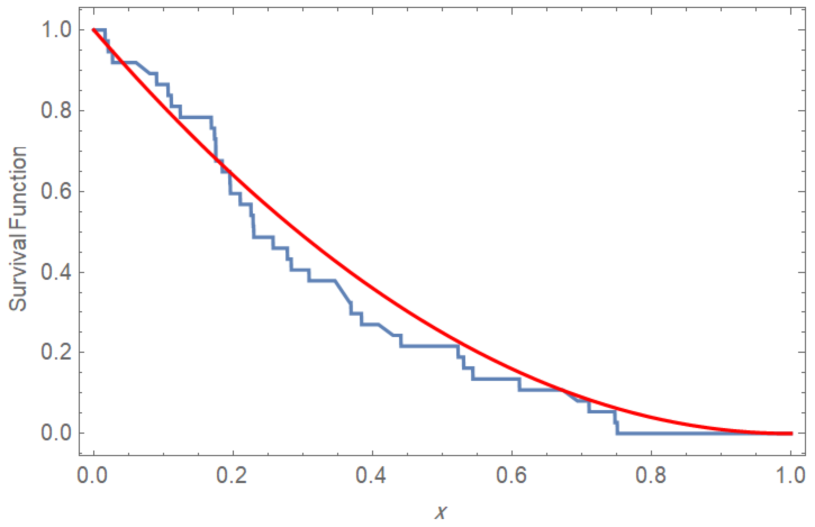
The UTLD was tested by the K-S test against the normalized censored values of survival times, as displayed in Figure 5. The computed value of the K-S test is $0.109063$ with a p-value equal to $0.730228$.

Figure 5. K-S test for censored survival data.

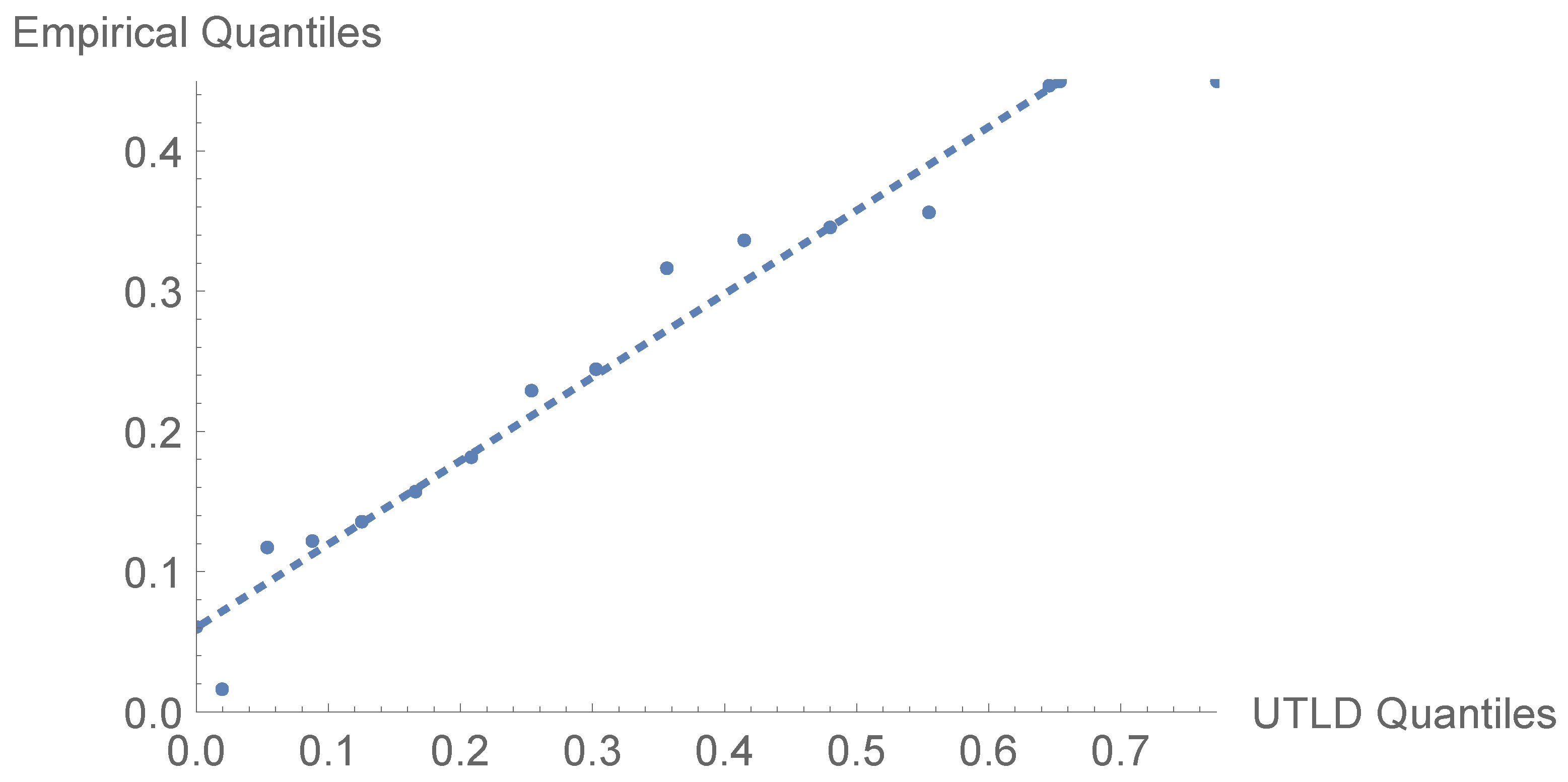
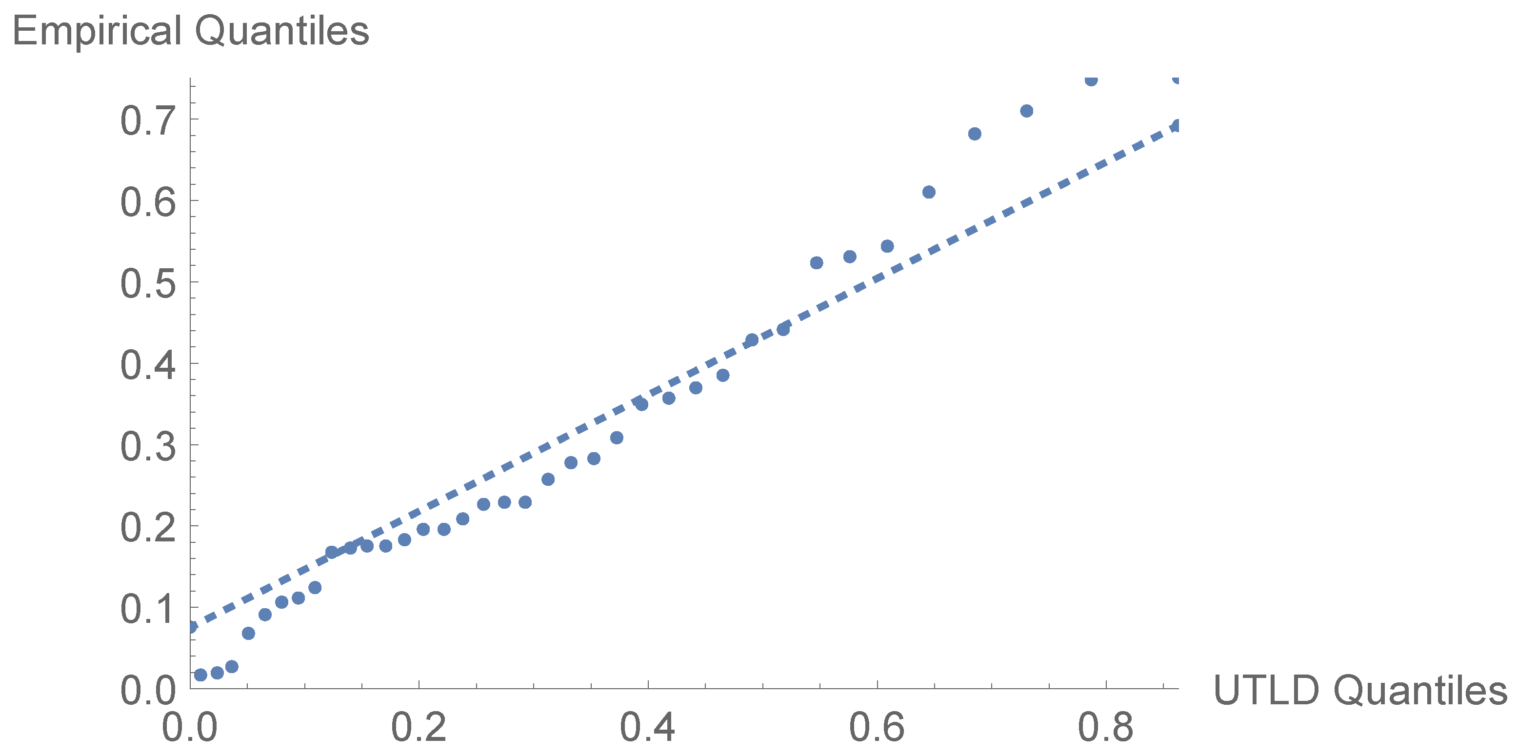
The normative Q-Q plot of censored survival times of UTLD is shown in Figure 6. Most of the range is covered by the points, which are very close to the diagonal line, indicating that the UTLD offers a suitable fit to the data on survival. Extreme quantile deviations are to be anticipated in censored survival samples, but generally, the linear trend indicates the strength and adaptability of the suggested model in dealing with skewed, constrained survival samples.

Figure 6. Q-Q plot for censored survival data.

The outcomes in Table 4 can be used to show that the suggested model is applicable to censored survival data. There are generally similarities in parameter estimates derived using various techniques, meaning that UTLD is robust in this regard. The broad MLE-confidence intervals, however, depict the uncertainty that is usually experienced in the case of a survival study, which is censoring. On the contrary, Bayesian credible intervals provide a tighter estimate, and those are simpler to interpret and more valuable in practical decision-making. In general, the results indicate that the UTLD is an effective and versatile model of modeling normalized censoring data.

Table 4. Extrapolated results from censored data.

Point Estimates of $\alpha$				Interval Estimates of $\alpha$
MLE	Bayesian SEL	Bayesian-LINEX Loss		CL	ACI	CRI
		$c_1=-2$	$c_2=2$	$90\%$	$0.509941,0.998067$	$0.884502,0.99635$
$0.75400$	$0.97868$	$0.97971$	$0.97754$	$95\%$	$0.575824,0.932183$	$0.870628,0.99635$

5. Conclusions

This study has developed a mathematical analysis of a J-shaped unit distribution by introducing and working out the unit Topp–Leone distribution. Analytical expressions have been given explicitly and with clear formulas for the most important distributional properties, such as moments, measures of entropy, order statistics, and L-moments, providing a transparent and reproducible framework for analysis. Under Type-II censoring, the study of statistical inference has been done with both classical and Bayesian methods with the help of simulation results, which explain the theoretical and practical performance of the estimators. The applications of the real data also show the effectiveness of the proposed model in the capture of the effect of boundaries and skewness in the limited data. The suggested framework also provides opportunities for future research, including extensions to regression structures, alternative censoring schemes, and additional theoretical generalizations in the category of unit distributions.

References

- Topp, C.W.; Leone, F.C. A Family of J-Shaped Frequency Functions. J. Am. Stat. Assoc. 1955, 50, 209–219. [Google Scholar] [CrossRef]
- Nadarajah, S.; Kotz, S. Moments of Some J-Shaped Distributions. J. Appl. Stat. 2003, 30, 311–317. [Google Scholar] [CrossRef] [Scilit]
- Afuecheta, E.; Okorie, I.E.; Jallow, H.; Nadarajah, S. A review of unit continuous probability distributions. AIMS Math. 2025, 10, 25939–26057. [Google Scholar] [CrossRef] [Scilit]
- Mazucheli, J.; Menezes, A.F.B.; Dey, S. Unit-Gompertz distribution with applications. Statistica 2019, 79, 25–43. [Google Scholar]
- Stojanović, V.S.; Bakouch, H.S.; Alomair, G.; Daghestani, A.F.; Grujčić, Ž. A Flexible Unit Distribution Based on a Half-Logistic Map with Applications in Stochastic Data Modeling. Symmetry 2025, 17, 278. [Google Scholar] [CrossRef] [Scilit]
- Al-Shomrani, A.; Arif, O.; Shawky, A.; Hanif, S.; Shahbaz, M.Q. Topp–Leone family of distributions: Some properties and application. Pak. J. Stat. Oper. Res. 2016, 12, 443–451. [Google Scholar] [CrossRef] [Scilit]
- Gradshteyn, I.S.; Ryzhik, I.M. Table of Integrals, Series, and Products, 7th ed.; Jeffrey, A., Zwillinger, D., Eds.; Academic Press: New York, NY, USA, 2007. [Google Scholar]
- Balakrishnan, N.; Cramer, E. The Art of Progressive Censoring; Birkhauser: New York, NY, USA, 2014. [Google Scholar] [CrossRef] [Scilit]
- Kundu, D.; Raqab, M.Z. Generalized Rayleigh distribution: Different methods of estimation. Comput. Stat. Data Anal. 2005, 49, 187–200. [Google Scholar] [CrossRef] [Scilit]
- Cover, T.M.; Thomas, J.A. Elements of Information Theory; John Wiley & Sons, Inc.: Hoboken, NJ, USA, 2006. [Google Scholar]
- Andrews, G.E.; Askey, R.; Roy, R. Special Functions; Cambridge University Press: Cambridge, UK, 1999. [Google Scholar] [CrossRef] [Scilit]
- Hosking, J.R.M. L-Moments: Analysis and Estimation of Distributions Using Linear Combinations of Order Statistics. J. R. Stat. Soc. Ser. B 1990, 52, 105–124. [Google Scholar] [CrossRef] [Scilit]
- Balakrishnan, N.; Aggarwala, R. Progressive Censoring: Theory, Methods and Applications; Birkhauser: Boston, MA, USA, 2000. [Google Scholar] [CrossRef] [Scilit]
- Al-Moisheer, A.S.; Sultan, K.S.; Mansour, M.M.M. A Fav-Jerry Distribution Under Joint Type-II Censoring: Quantifying Cross-Cultural Differences in Autism Knowledge. Math. Comput. Appl. 2025, 30, 120. [Google Scholar] [CrossRef] [Scilit]
- Cohen, A.C. Maximum likelihood estimation in the Weibull distribution based on complete and on censored samples. Technometrics 1965, 7, 579–588. [Google Scholar] [CrossRef]
- Seiffert, S.S.; Weber, S.W.S.; Sack, U.S.; Keller, T.K. Use of logit transformation within statistical analyses of experimental results obtained as proportions: Example of method validation experiments and EQA in flow cytometry. Front. Mol. Biosci. 2024, 11, 1335174. [Google Scholar] [CrossRef] [Scilit] [PubMed]
- Casella, G.; Berger, R.L. Statistical Inference, 2nd ed.; Duxbury Press: Pacific Grove, CA, USA, 2002. [Google Scholar]
- Al-Moisheer, A.S.; Sultan, K.S.; Mansour, M.M.M. Bayesian and Classical Inferences of Two-Weighted Exponential Distribution and Its Applications to HIV Survival Data. Symmetry 2026, 18, 96. [Google Scholar] [CrossRef] [Scilit]
- Elzaki, R.M.; Al-Mahish, M. Food insecurity and water management shocks in Saudi Arabia: Bayesian VAR analysis. PLoS ONE 2024, 19, E0296721. [Google Scholar] [CrossRef] [PubMed]
- Laha, R.G. Characteristic functions. In Encyclopedia of Statistical Sciences; Kotz, S., Johnson, N., Eds.; John Wiley & Sons: New York, NY, USA, 1982; Volume 1, pp. 415–422. [Google Scholar]
Disclaimer/Publisher’s Note: The statements, opinions and data contained in all publications are solely those of the individual author(s) and contributor(s) and not of MDPI and/or the editor(s). MDPI and/or the editor(s) disclaim responsibility for any injury to people or property resulting from any ideas, methods, instructions or products referred to in the content. |
© 2026 by the authors. Licensee MDPI, Basel, Switzerland. This article is an open access article distributed under the terms and conditions of the Creative Commons Attribution (CC BY) license.