Solving the Road-Rail Intermodal Network Design Problem: A Novel 0-1 Nonlinear Model to Consider Carbon Emission Policies

Abstract

In recent years, climate change has become increasingly urgent, and governments are intensifying efforts to regulate carbon-intensive industries through policy innovations. The transport sector faces particularly acute decarbonisation challenges due to its reliance on fossil fuels. This study investigates road-rail intermodal transport as a strategic solution that synergises the flexibility of trucking with the superior energy efficiency of rail. A novel arc-path 0-1 nonlinear model is developed, optimising profit maximisation while incorporating hard constraints on transport due dates. The predominant carbon emission policies—command-and-control regulations and carbon pricing mechanisms—are analysed, and the corresponding extended models are constructed. Next, the linearisation techniques are introduced. In the end, a numerical example is built to test the validity of the model and compare the optimisation decisions of the basic model and the extended models. Furthermore, a sensitivity analysis of key parameters is conducted to provide operational recommendations for enterprises to balance carbon emissions and profits.

1. Introduction

The growing urgency of climate change has compelled governments worldwide to implement stringent carbon emission policies, such as carbon tax, Emissions Trading System (ETS), and emission reduction targets. The global transport sector, responsible for 23% of energy-related carbon dioxide (CO₂) emissions, faces immense pressure to decarbonise. According to the International Energy Agency (IEA), CO₂ emissions from the transport sector must decline by over 3% annually through 2030 to align with the Net Zero Emissions (NZE) by 2050 scenario. In China, road freight accounts for 30.73% of total freight volume by tonne–kilometres, according to data published by the National Bureau of Statistics of China in 2023. However, road transport generates over 80% of the transport sector’s emissions, whereas rail, handling 10% of freight volume, contributes a mere 0.7% of emissions. This disparity arises because rail transport emits 75% less CO₂ per tonne–kilometre than road transport. This misalignment between freight volume share and emission contributions underscores the urgency of modal shifts. Governments have been prompted to incentivise modal shifts in transport through carbon emission policies (e.g., EU ETS). Road-rail intermodal transport, which strategically combines the flexibility of first/last-mile trucking with the energy efficiency of long-haul rail, has emerged as a promising solution to decarbonise operations without compromising efficiency. However, designing such networks under evolving carbon emission policies presents complex challenges, including balancing infrastructure costs, freight revenues, carbon costs, and service reliability.

Existing studies on Service Network Design Problems (SNDP) have predominantly focused on cost minimisation or profit maximisation, treating environmental impacts as secondary constraints. Although recent works have incorporated carbon emissions into optimisation models, most of them simply consider the carbon emissions cost in the system of the objective function or impose static emission caps as constraints, and very few studies have addressed the impacts of different carbon emission policies on the road-rail intermodal network design. This paper aims to demonstrate a novel mathematical optimisation model that can be employed by freight carriers to balance profit and carbon emissions, to offer practical insights into the effect of different carbon emission policies on road-rail intermodal network design, and to better meet market and environmental needs.

The remainder of this paper is organised as follows: Section 2 summarises relevant studies about SNDP; Section 3 briefly describes the transport strategy in road-rail intermodal networks; in Section 4, we propose the basic model formulation and extended models based on carbon emission policies, as well as the linearisation techniques; and finally, a numerical example and conclusions are given in Section 5 and Section 6, respectively.

2. Literature Review

The SNDP, a pivotal medium-term tactical planning challenge in freight transport systems [1] (Assad, 1980), has attracted substantial scholarly attention since its conceptualisation. It focuses on how to utilise limited resources to achieve the displacement of cargo flows, primarily involving decisions related to transport service operation and cargo flow distribution [2] (Wang, Qi, Cheng, and Zhang, 2019), usually with the objective of cost minimisation or profit maximisation. As early as the 1980s, intercity freight network models were summarised by Friesz, Tobin, and Harker [3] (1983). Later, Crainic [4] (2000) formalised the SNDP as a comprehensive methodology for addressing carrier-specific tactical decisions. He argued that the SNDP models were classified into frequency and dynamic models, with the latter not only considering the frequency of freight service but also the temporal dimensions, i.e., satisfying the spatiotemporal transport requirements. Subsequent extensions integrated vehicle fleet management and crew scheduling into the SNDP framework [5] (Wieberneit, 2008). Some scholars view the SNDP as a multi-commodity flow problem [6] (Pedersen, Crainic, and Madsen, 2009), which can be categorised into two principal variants: the uncapacitated and capacitated network design problems. Regarding the former, Balakrishnan, Magnanti, and Wong [7] (1989) designed a family of dual-ascent algorithms, while Holmberg and Hellstrand [8] (1998) proposed a Lagrangian heuristic and branch-and-bound to find the exact optimal solution. As for the latter, Lamar, Sheffi, and Powell [9] (1990) introduced the capacity improvement bound and developed an implementation scheme using shortest path and linearised knapsack programmes. Subsequently, Holmberg and Yuan [10] (2000) presented a solution approach combining a Lagrangian heuristic and branch-and-bound. In recent studies, the network design problem has also been examined from the perspective of decision-variable characteristics. Kalantari, Mirzahossein, Najafi, Waller, and Zhang [11] (2023) distinguished between continuous and discrete network design problems according to whether link capacity decisions are modelled as continuous or binary variables and developed an efficient partially linearised subgradient algorithm for the continuous network design problem (CNDP). Addressing the discrete variant of the problem, Mirzahossein, Najafi, Kalantari, and Waller [12] (2025) proposed a deterministic solution framework for the discrete network design problem (DNDP), integrating disjunctive programming with an improved partially linearised subgradient method to enhance computational efficiency while maintaining solution quality. These studies provide a broader methodological context for network design modelling by highlighting how different decision structures influence problem formulation and solution strategies, which is also relevant to the SNDP involving discrete operational decisions.

Several efforts have been directed toward the formulation of models. Among these studies, Crainic and Rousseau [13] (1986) presented a general network optimisation modelling framework to determine the frequency of each selected service, which established a typical frequency service network design formulation for multimodal multicommodity freight transport. For scenarios with fixed resources, Kim and Barnhart [14] (1999) introduced a general modelling framework to optimise the transport services and schedules for the large-scale service network. Crainic, Hewitt, Toulouse, and Vu [15] (2016) argued that resources have a cycle-based nature, i.e., resources are limited in each terminal, and a resource must ultimately return to its assigned terminal. Based on this, they proposed a new SNDP model to simultaneously determine services provided, commodity routes, and resource routes. There are two main types of existing model formulations, namely the arc-based and cycle-based models. Andersen, Crainic, and Christiansen [16] (2009) compared model formulations using arc variables, path flow variables, and novel cycle design variables, analysing the strengths and weaknesses of each. Both Pedersen et al. [6] (2009) and Li, Ding, Pan, Jiang, and Aneja [17] (2020) constructed arc-based and cycle-based formulations incorporating the resource constraints at terminals, with the latter additionally addressing single-path requirements into account. A tabu search metaheuristic framework [6] (Pedersen et al., 2009) and a two-stage mathematical integer programming-based heuristic [17] (Li et al., 2020) were designed for the arc-based model and the cycle-based model, respectively. For less-than-truckload (LTL) carriers, Jiang, Bai, Atkin, and Kendall [18] (2017) transformed the solution network of the arc-based SNDP model into a set of cyclic routes that cover all arcs in the network to assign a cyclic route to each vehicle.

Furthermore, some scholars have focused on the impact of asset management. SNDP with asset management comprises two related subproblems: the service network design problem and the asset assignment problem, and most studies primarily focus on vehicles. Teypaz, Schrenk, and Cung [19] (2010) developed a three-step decomposition heuristic, i.e., network construction, vehicle loading, and vehicle scheduling, to maximise carrier profitability. Li, Wei, Aneja, and Tian [20] (2017) focused on the impact of heterogeneous asset management in the design-balanced capacitated multicommodity network design problem. Wang et al. [2] (2019) proposed arc-based and cycle-path models for the heterogeneous fleet issue to simultaneously optimise transport services, commodity flows, and heterogeneous fleet sizing. Scherr, Saavedra, Hewitt, and Mattfeld [21] (2019) examined tactical planning for parcel delivery using autonomous vehicles (AVs) and manually operated vehicles (MOVs). In their vision, AVs are restricted to predefined operational zones, while they should be guided by MOVs in platoons outside these zones. A time-expanded network was introduced, and an integer linear programme was formulated to decide the fleet size and mix, as well as the routing of cargoes and vehicles.

The SNDP has been widely applied in multiple transport fields and can be categorised into single-mode and intermodal transport systems. Given that this paper focuses on the road-rail intermodal transport networks, we primarily present an overview of rail transport, road transport, and intermodal transport systems.

Barnhart, Jin, and Vance [22] (2000) viewed the blocking problem in rail transport as an SNDP with maximum-degree and flow constraints, proposing a heuristic Lagrangian relaxation approach that decomposed the original mixed integer programming problem into two simple subproblems. Considering the handling cost and the movements of full and empty railcars, Lulli, Pietropaoli, and Ricciardi [23] (2011) formulated a minimum concave-cost function to simultaneously determine: (1) services provided, (2) train quantities per path, and (3) railcar numbers/types. To satisfy the spatiotemporal requirements in freight rail transport, Zhu, Crainic, and Gendreau [24] (2014) integrated service selection/scheduling, car classification/blocking, train make-up, and shipment routing based on a proposed three-layer space-time network. Regarding passenger transport, López-Ramos, Codina, Marín, and Guarnaschelli [25] (2017) combined the transit network design problem and transit frequency setting problem via an optimisation-based approach to balance passenger riding time minimisation against operator cost minimisation.

In road transport, services can be categorised into less-than-truckload [26] (LTL) (Jarrah, Johnson, and Neubert, 2009) and full truckload [27] (FTL) (Grimault, Bostel, and Lehuédé, 2017). Farvolden and Powell [28] (1994) developed local-improvement heuristics for SNDP in the motor carrier industry, considering capacity constraints in the shipment routing subproblem, which was formulated as a multi-commodity network flow problem. Sung and Song [29] (2003) proposed a path-based model to determine direct services and vehicle allocation for given freight demands while incorporating vehicle capacity and service time constraints within a cross-docking supply chain network. In addition, SNDP under uncertain demand is also a popular research direction. Lium, Crainic, and Wallace [30] (2009) demonstrated that the transport plan would be more robust when based on stochastic demand patterns, with consolidation serving as an effective hedge against uncertainty. Bai, Wallace, Li, and Chong [31] (2014) adopted rescheduling to deal with uncertainties and constructed a stochastic freight service network design model in which a set of integer variables for vehicle rerouting was established to improve network flexibility and balance the conflict between low network setup costs and low expected operational costs. Substantial research exists in other transport domains: Van, Gao, Leung, and Wallace [32] (2014) and Yu, Yang, and Yu [33] (2017) investigated flight network optimisation; Lai and Lo [34] (2004) along with Lo, An, and Lin [35] (2013) examined ferry network design, while Yang, Pan, and Wang [36] (2018), Reinhardt, Pisinger, Sigurd, and Ahmt [37] (2020), and Meng and Wang [38] (2011) conducted studies on liner shipping networks.

As intermodal transport plays a critical role in modern transport systems, it has attracted significant research attention in the SNDP. Kim, Barnhart, Ware, and Reinhardt [39] (1999) developed a model for large-scale express package delivery networks that sought to minimise transport costs while accommodating tight service windows, limited sort capacity, and vehicle/aircraft availability constraints. Riessen, Negenborn, Dekker, and Lodewijks [40] (2015) formulated a model for intermodal container networks integrating barge, rail, and truck services, especially incorporating flexibility for overdue delivery and hybrid use of self-operated/subcontracted slots to optimise service timetables. Similarly, Farahani, Noble, McGarvey, and Enayati [41] (2023) established an advanced intermodal service network model that accounted for overdue costs, modal integration, resource constraints, and time windows to determine optimal transport paths for the synchro-modal transport system. Laaziz and Sbihi [42] (2019) investigated the SNDP for intermodal rail-road container freight transport through a capacitated fixed charge path formulation to simultaneously determine service frequency, terminal loading plans, and required capacity of each terminal. Regarding uncertainty management, Demir et al. [43] (2016) and Uddin and Huynh [44] (2019) explored SNDP variants under uncertain scenarios, with the former addressing travel time and demand fluctuations, while the latter focused on capacity uncertainty. With a growing emphasis on sustainability, Bouchery and Fransoo [45] (2015) examined the changing dynamics of intermodal transport solutions from the perspective of cost, carbon emissions, and modal shift. Their findings revealed that maximising modal shifts could paradoxically increase both cost and carbon emissions, highlighting the need for balanced optimisation approaches. Inghels, Dullaert, and Vigo [46] (2016) proposed a dynamic tactical planning model with multimodal truck and inland water transport to achieve a shift from road to water transport, aiming at minimising the sum of transport costs, greenhouse gas emission costs, and societal costs. Lam and Gu [47] (2016) analysed the effect of different carbon emission restrictions and proposed a bi-objective optimisation model to minimise cost and time.

In this study, we investigate the road-rail intermodal network design problem for freight carriers, taking carbon emission policies into account. The concrete contributions of the work can be summarised as follows.

(1) Unlike prior studies that predominantly focused on the carbon emission cost or restricted emission zones, we propose a flexible model capable of adapting to diverse carbon emission policies, e.g., carbon tax and ETS. This innovation enables carriers to quantitatively evaluate trade-offs between emission reduction targets and network operational efficiency.

(2) Recognising that cargo owners have different requirements for the deadline for delivery of cargo, we formulate an arc-path 0-1 nonlinear programming model considering the transport due date constraints to determine the services provided, the service frequency, and the cargo flow assignment plans in the road-rail intermodal network. This formulation addresses the operational complexity faced by carriers in balancing service reliability with cost-effectiveness.

(3) We consider the existence of two types of heterogeneous trains, i.e., express trains and ordinary trains, and the mutual attraction of cargo flows between express trains and ordinary trains, which is ignored in real-world intermodal operations.

3. The Analysis of Road-Rail Intermodal Transport Strategy

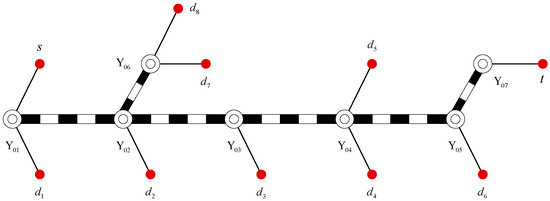
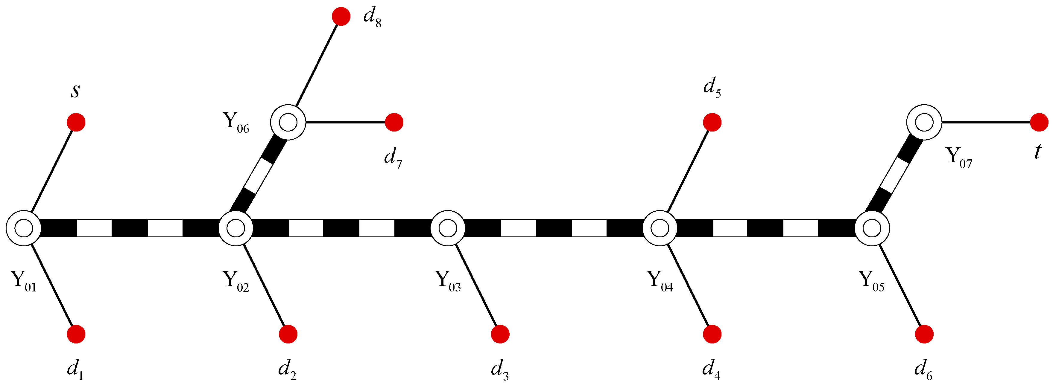
To capture market share in high-value cargo transport, railroad operators have implemented different grades of express train services between marshalling yards (or logistics hubs). These facilities, functioning as network nodes rather than direct demand sources, require integration with road feeder systems. The resultant road-rail intermodal network enables convenient ‘door-to-door’ services through coordinated modal transfers. This section demonstrates the intermodal transport strategies using a network of seven hubs (see Figure 1).

Figure 1. The road-rail intermodal network.

The road-rail intermodal network is a typical hub-and-spoke network structure where the marshalling yards (${\mathrm{Y}}_{01}$–${\mathrm{Y}}_{05}$) and logistics hubs (${\mathrm{Y}}_{06}$, ${\mathrm{Y}}_{07}$) function as consolidation centres, demand nodes ($s$, $t$, $d_1$–$d_8$) are exclusively assigned to a single hub. Connectivity between demand nodes is ensured through direct road transport. In addition, rail freight services are provided, including ordinary trains (Light orange arcs) with a formulation plan of ${\mathrm{Y}}_{01}\to {\mathrm{Y}}_{02}$, of ${\mathrm{Y}}_{02}\to {\mathrm{Y}}_{03}$, of ${\mathrm{Y}}_{03}\to {\mathrm{Y}}_{04}$, and of ${\mathrm{Y}}_{04}\to {\mathrm{Y}}_{05}$, express trains with an operation plan of ${\mathrm{Y}}_{01}\to {\mathrm{Y}}_{02}\to {\mathrm{Y}}_{05}$ (Bright pink arcs), of ${\mathrm{Y}}_{01}\to {\mathrm{Y}}_{03}\to {\mathrm{Y}}_{05}$ (Dusty purple arcs), of ${\mathrm{Y}}_{06}\to {\mathrm{Y}}_{05}$ (Yellow arc), of ${\mathrm{Y}}_{02}\to {\mathrm{Y}}_{04}\to {\mathrm{Y}}_{07}$ (Dark red arcs), of ${\mathrm{Y}}_{05}\to {\mathrm{Y}}_{07}$ (Khaki arc) and of ${\mathrm{Y}}_{01}\to {\mathrm{Y}}_{07}$ (Olive green arc). The road-rail intermodal transport strategy is discussed for the shipment $N_{st}$ (but is not limited to), see Figure 2.

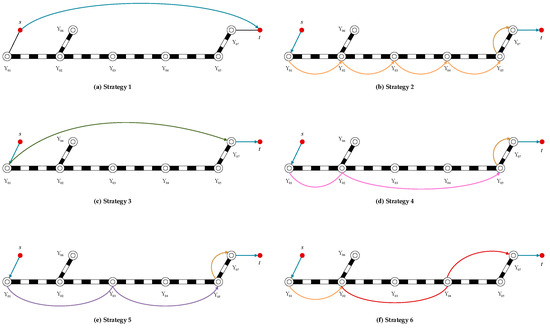
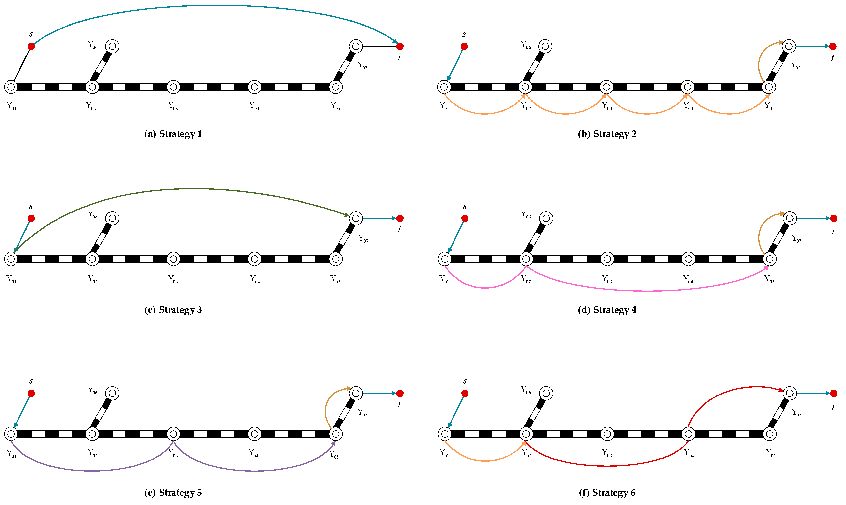
Figure 2. The road-rail intermodal transport strategy for shipment $N_{st}$.

Strategy 1 (see Figure 2a): $N_{st}$ is transported to the destination $t$ by direct road service.

Strategy 2 (see Figure 2b): $N_{st}$ is transported to the hub ${\mathrm{Y}}_{01}$ by road transport, and then arrives at the hub ${\mathrm{Y}}_{07}$ through a series of ordinary train services and express train services, ${\mathrm{Y}}_{01}\to {\mathrm{Y}}_{02}$, ${\mathrm{Y}}_{02}\to {\mathrm{Y}}_{03}$, ${\mathrm{Y}}_{03}\to {\mathrm{Y}}_{04}$, ${\mathrm{Y}}_{04}\to {\mathrm{Y}}_{05}$, and ${\mathrm{Y}}_{05}\to {\mathrm{Y}}_{07}$, respectively. Finally, it is transported to its destination $t$ by road transport.

Strategy 3 (see Figure 2c): $N_{st}$ is transported to the hub ${\mathrm{Y}}_{01}$ by road transport first, then arrives at the hub ${\mathrm{Y}}_{07}$ through express train service ${\mathrm{Y}}_{01}\to {\mathrm{Y}}_{07}$, and finally is transported to the destination $t$ by road transport.

Strategy 4 (see Figure 2d): Similarly, $N_{st}$ is transported to the hub ${\mathrm{Y}}_{01}$ by road transport firstly, and then is transported to the hub ${\mathrm{Y}}_{05}$ through express train service ${\mathrm{Y}}_{01}\to {\mathrm{Y}}_{02}\to {\mathrm{Y}}_{05}$, then reaches the hub ${\mathrm{Y}}_{07}$ by express train service ${\mathrm{Y}}_{05}\to {\mathrm{Y}}_{07}$, and finally, arrives at the destination $t$ by road transport.

Strategy 5 (see Figure 2e): $N_{st}$ is transported to the hub ${\mathrm{Y}}_{01}$ by road transport, then reaches the hub ${\mathrm{Y}}_{05}$ through express train service ${\mathrm{Y}}_{01}\to {\mathrm{Y}}_{03}\to {\mathrm{Y}}_{05}$, then arrives at the hub ${\mathrm{Y}}_{07}$ by express train service ${\mathrm{Y}}_{05}\to {\mathrm{Y}}_{07}$, and finally arrives at the destination $t$ by road transport.

Strategy 6 (see Figure 2f): Firstly, $N_{st}$ is transported to the hub ${\mathrm{Y}}_{01}$ through road transport, and then arrives at the hub ${\mathrm{Y}}_{02}$ and hub ${\mathrm{Y}}_{07}$ successively, through ordinary train service ${\mathrm{Y}}_{01}\to {\mathrm{Y}}_{02}$ and express train service ${\mathrm{Y}}_{02}\to {\mathrm{Y}}_{04}\to {\mathrm{Y}}_{07}$, and finally is transported to the destination $t$ through road transport.

In the proposed strategies, only Strategy 1 adopts single-mode road transport, while the remaining strategies involve road-rail intermodal transport. Specifically, Strategy 2 requires six transshipment operations (the maximum) at intermediate hubs, whereas in Strategy 3, only two transshipments at hubs ${\mathrm{Y}}_{01}$ and ${\mathrm{Y}}_{07}$ are carried out, and Strategies 4–6 all involve four transshipment operations. Increased transshipment operations inherently extend total transport time, a key factor in service selection due to time-sensitive delivery requirements. The excessive transshipment operations significantly elevate the risk of exceeding contractual delivery windows. Consequently, Strategy 2 may prove operationally infeasible for urgent shipments, despite potential cost advantages. While rail transport offers economies of scale, its sequential loading/unloading introduces temporal penalties that road-dominated strategies avoid.

Furthermore, the implementation of carbon emission policies exerts a significant influence on transport modal selection due to varying carbon emission levels across different strategies. Taking Strategy 1 as a representative case, while maintaining its position as the most convenient freight service with optimal transit duration, this road-dominated strategy incurs substantially higher carbon emissions compared to rail-based alternatives. Consequently, its economic viability diminishes under the carbon tax and ETS, as operational costs increase. This study systematically investigates the impact of carbon emission policies on road-rail intermodal network design, developing the corresponding mathematical models that ensure carrier profit maximisation, taking the cargo transport due date into account.

4. Model Formulation for the Road-Rail Intermodal Network Design Problem

In this section, a mathematical optimisation model for road-rail intermodal network design will be developed, with the objective of maximising the freight profit for carriers. The model formulation addresses three critical operational decisions: (1) selection of freight service types to be provided, (2) determination of service frequencies, and (3) assignment of service arcs to cargo flows. Furthermore, carbon emission policies are systematically integrated into the framework to evaluate their operational implications on intermodal network optimisation.

4.1. Model Hypothesis

The model formulation is subject to the following assumptions:

(1) The physical path of each shipment is predetermined;

(2) Shipments with the same origin–destination (OD) pairs must be transported by the same freight services, which means they cannot be split during the transport process;

(3) The number of marshalling railcars is predetermined, and road transport employs homogeneous truck fleets;

(4) The transfer time between rail transport and road transport is constant.

(5) The topological structure of the road-rail intermodal network is predetermined during the planning horizon.

It should be noted that, although carbon emission policies may in practice influence truck demand and route choices, such behavioural adjustments are not considered in this study. The model focuses on the road-rail intermodal service network, specifically on service type selection, service frequencies, and freight profit for carriers. These assumptions define the scope of the current analysis, and the potential impact of truck route or demand adjustments could be explored in future research.

4.2. Notations and Definitions

The notations and definitions involved in the model are as follows.

Sets	Definition
$V^{\mathrm{Hub}}$	Set of hubs in the network, including marshalling yards and logistics hubs, $i,j,u\in V^{\mathrm{Hub}}$
$V^{\mathrm{Rail}}$	Set of marshalling yards in the network, $i^{\prime },j^{\prime }\in V^{\mathrm{Rail}}$, $V^{\mathrm{Rail}}\subset V^{\mathrm{Hub}}$
$V^{\mathrm{Log}}$	Set of logistics hubs in the network, $i^{″},j^{″}\in V^{\mathrm{Log}}$, $V^{\mathrm{Log}}\subset V^{\mathrm{Hub}}$
$V^{\mathrm{Spoke}}$	Set of non-hub nodes in the network, i.e., road terminals, $s,t\in V^{\mathrm{Spoke}}$
$E^{\mathrm{Rail}}$	Set of rail physical arcs in the network, $m\in E^{\mathrm{Rail}}$
$A^{\mathrm{Rail}}$	Set of rail service arcs in the network, $a\in A^{\mathrm{Rail}}$
$G$	Set of grades of express trains, $g\in G$
$E$	The candidate set of express train services, $e\in E$
$A_e^{\mathrm{Rail}}$	Set of rail service arcs corresponding to express train services, $ae\in A_e^{\mathrm{Rail}}$
$K$	The candidate set of ordinary train services, $k\in K$
$A_k^{\mathrm{Rail}}$	Set of rail service arcs corresponding to ordinary train services, $ak\in A_k^{\mathrm{Rail}}$
Parameters	Definition
$s_a$	The tail node of the rail service arc $a$, $s_a\in V^{\mathrm{Hub}}$, $a\in A^{\mathrm{Rail}}$
$t_a$	The head node of the rail service arc $a$, $t_a\in V^{\mathrm{Hub}}$, $a\in A^{\mathrm{Rail}}$
$d_{st}$	Freight transport demand from road terminal $s$ to $t$, $s,t\in V^{\mathrm{Spoke}}$, in tons per day
$T_{st}$	Transport due date of shipment from road terminal $s$ to $t$, $s,t\in V^{\mathrm{Spoke}}$, in hours
$C{R}_{i^{\prime }}$	The maximum operating capacity of the marshalling yard $i^{\prime }$, $i^{\prime }\in V^{\mathrm{Rail}}$, in railcars per day
$C{L}_{i^{″}}$	The maximum operating capacity of the logistics hub $i^{″}$, $i^{″}\in V^{\mathrm{Log}}$, in railcars per day
$\theta$	Conversion coefficient of the original operating capacity of hub
$m_{ij}$	Average number of marshalling railcars, including ordinary trains and express trains, $i,j\in V^{\mathrm{Hub}}$, in railcars
$D^{\mathrm{Truck}}$	The average static load of trucks, in tons per truck
$P$	The average static load of railcars, in tons per railcar
$l_s^i$	Distance between road terminal $s$ and hub $i$, $i\in V^{\mathrm{Hub}},s\in V^{\mathrm{Spoke}}$, in kilometres
$l_s^t$	Distance between the road terminal $s$ and $t$, $s,t\in V^{\mathrm{Spoke}}$, in kilometres
$l_m$	Length of rail physical arc $m$, $m\in E^{\mathrm{Rail}}$, in kilometres
$v^{\mathrm{Truck}}$	The average speed of trucks, in kilometres per hour
$v^{\mathrm{Ord}}$	The average speed of ordinary trains, in kilometres per hour
$v_g$	The average speed of express trains with grade $g$, $g\in G$, in kilometres per hour
${\tau }_i$	Average transfer time at the hub $i$ between road transport and rail transport, $i\in V^{\mathrm{Hub}}$, in hours
$\tau$	Average transfer time between consecutive rail service arcs, in hours
${\tau }_a$	Transport time on rail service arc $a$, $a\in A^{\mathrm{Rail}}$, in hours
${\varpi }^{\mathrm{Truck}}$	Unit freight revenue of trucks, in CNY per tonne–kilometre
${\varpi }_g$	Unit freight revenue of express train services with the grade $g$, $g\in G$, in CNY per tonne–kilometre
${\varpi }^{\mathrm{Ord}}$	Unit freight revenue of ordinary trains, in CNY per tonne–kilometre
$C^{\mathrm{Fix-truck}}$	Fixed operational cost of trucks, in CNY per truck
$C_g^{\mathrm{Fix}}$	Fixed operational cost of express trains with grade $g$, $g\in G$, in CNY per train
$C^{\mathrm{Fix-ord}}$	Fixed operational cost of ordinary trains, in CNY per train
$C^{\mathrm{Km-truck}}$	Travelling cost of trucks, in CNY per truck-kilometre
$C_g^{\mathrm{Km}}$	Travelling cost of express trains with grade $g$, $g\in G$, in CNY per train-kilometre
$C^{\mathrm{Km-ord}}$	Travelling cost of ordinary trains, in CNY per train-kilometre
${\alpha }_e^{ae}$	It takes value 1 if express service arc $ae$ is included in express service $e$, otherwise it is 0, $ae\in A_e^{\mathrm{Rail}}$, $e\in E$
${\beta }_k^{ak}$	It takes value 1 if ordinary service arc $ak$ is included in ordinary service $k$, otherwise it is 0, $ak\in A_k^{\mathrm{Rail}}$, $k\in K$
${\eta }_{ae}^m$	It takes value 1 if rail physical arc $m$ is contained by express service arc $ae$, otherwise it is 0, $ae\in A_e^{\mathrm{Rail}}$, $m\in E^{\mathrm{Rail}}$
${\eta }_{ak}^m$	It takes value 1 if rail physical arc $m$ is contained by ordinary service arc $ak$, otherwise it is 0, $ak\in A_k^{\mathrm{Rail}}$, $m\in E^{\mathrm{Rail}}$
${\delta }_s^i$	It takes value 1 if road terminal $s$ is connected to hub $i$, otherwise it is 0, $s\in V^{\mathrm{Spoke}}$, $i\in V^{\mathrm{Hub}}$
$f⌈·⌉$	The ceiling function
$M$	A sufficiently large positive constant
Decision variables	Definition
$x_k$	Ordinary train variable; it takes value 1 if ordinary service $k$ is provided, otherwise it is 0
$y_g^e$	Express train variable; it takes value 1 if express service $e$ with grade $g$ is provided, otherwise it is 0
$z_{st}^{gae}$	Railcar flow variable; it takes value 1 if shipment from $s$ to $t$ uses express service arc $ae$ with grade $g$, otherwise it is 0
$z_{st}^{ak}$	Railcar flow variable; it takes value 1 if shipment from $s$ to $t$ uses ordinary service arc $ak$, otherwise it is 0
$z_{st}$	Truck flow variable; it takes value 1 if shipment from $s$ to $t$ chooses direct road transport, otherwise it is 0
$z_s^i$	Truck flow variable; it takes value 1 if shipment is transported from road terminal $s$ to hub $i$, otherwise it is 0
$z_j^t$	Truck flow variable; it takes value 1 if shipment is transported from hub $j$ to road terminal $t$, otherwise it is 0

4.3. Basic Model Formulation

Based on the notations described above, the optimisation model for the road-rail intermodal network design (RRIND) is constructed.

(RRIND)

$$\max Z=Z_1+Z_2+Z_3-Z_4-Z_5-Z_6$$

(1)

$\mathrm{s}.\mathrm{t}.$

$${\displaystyle \sum _{g\in G}{y}_g^e}\le 1\hspace{1em}\forall e\in E$$

(2)

$$z_{st}+{\displaystyle \sum _{i,j\in V^{\mathrm{Hub}}}{z}_s^i{\delta }_s^i{z}_j^t{\delta }_t^j}=1\hspace{1em}\forall s,t\in V^{\mathrm{Spoke}}$$

(3)

$${\displaystyle \sum _{i\in V^{\mathrm{Hub}}}{z}_s^i{\delta }_s^i}={\displaystyle \sum _{j\in V^{\mathrm{Hub}}}{z}_j^t{\delta }_t^j}\hspace{1em}\forall s,t\in V^{\mathrm{Spoke}}$$

(4)

$$z_{st}+{\displaystyle \sum _{i\in V^{\mathrm{Hub}}}\left({\displaystyle \sum _{g\in G}{\displaystyle \sum _{e\in E}{\displaystyle \sum _{ae:s_{ae}=i}{\delta }_s^i{y}_g^e{\alpha }_e^{ae}{z}_{st}^{gae}}}}+{\displaystyle \sum _{k\in K}{\displaystyle \sum _{ak:s_{ak}=i}{\delta }_s^i{x}_k{\beta }_k^{ak}{z}_{st}^{ak}}}\right)}=1\hspace{1em}\forall s,t\in V^{\mathrm{Spoke}}$$

(5)

$$z_{st}+{\displaystyle \sum _{j\in V^{\mathrm{Hub}}}\left({\displaystyle \sum _{g\in G}{\displaystyle \sum _{e\in E}{\displaystyle \sum _{ae:t_{ae}=j}{\delta }_t^j{y}_g^e{\alpha }_e^{ae}{z}_{st}^{gae}}}}+{\displaystyle \sum _{k\in K}{\displaystyle \sum _{ak:t_{ak}=j}{\delta }_t^j{x}_k{\beta }_k^{ak}{z}_{st}^{ak}}}\right)=1}\hspace{1em}\forall s,t\in V^{\mathrm{Spoke}}$$

(6)

$$\begin{array}{c}0\le {\displaystyle \sum _{i,j\in V^{\mathrm{Hub}}}{\displaystyle \sum _{g\in G}{\displaystyle \sum _{e\in E}{\displaystyle \sum _{k\in K}{\displaystyle \sum _{ae:t_{ae}=u}{\displaystyle \sum _{ak:t_{ak}=u}{\delta }_s^i{\delta }_t^j\left(x_k{\beta }_k^{ak}{z}_{st}^{ak}+y_g^e{\alpha }_e^{ae}{z}_{st}^{gae}\right)}}}}}}\le 1\\ \forall s,t\in V^{\mathrm{Spoke}},u\in V^{\mathrm{Hub}},u\ne i,j\end{array}$$

(7)

$$\begin{array}{c} {\displaystyle \sum _{i,j\in V^{\mathrm{Hub}}}{\displaystyle \sum _{g\in G}{\displaystyle \sum _{e\in E}{\displaystyle \sum _{k\in K}{\displaystyle \sum _{ae:t_{ae}=u}{\displaystyle \sum _{ak:t_{ak}=u}{\delta }_s^i{\delta }_t^j\left(x_k{\beta }_k^{ak}{z}_{st}^{ak}+y_g^e{\alpha }_e^{ae}{z}_{st}^{gae}\right)}}}}}}\\ ={\displaystyle \sum _{i,j\in V^{\mathrm{Hub}}}{\displaystyle \sum _{g\in G}{\displaystyle \sum _{e\in E}{\displaystyle \sum _{k\in K}{\displaystyle \sum _{ae:s_{ae}=u}{\displaystyle \sum _{ak:s_{ak}=u}{\delta }_s^i{\delta }_t^j\left(x_k{\beta }_k^{ak}{z}_{st}^{ak}+y_g^e{\alpha }_e^{ae}{z}_{st}^{gae}\right)}}}}}}\\ \forall s,t\in V^{\mathrm{Spoke}},u\in V^{\mathrm{Hub}},u\ne i,j\end{array}$$

(8)

$${\displaystyle \sum _{e\in E}{y}_g^e{\alpha }_e^{ae}}\ge z_{st}^{gae}\hspace{1em}\forall s,t\in V^{\mathrm{Spoke}},ae\in A_e^{\mathrm{Rail}},g\in G$$

(9)

$${\displaystyle \sum _{k\in K}{x}_k{\beta }_k^{ak}}\ge z_{st}^{ak}\hspace{1em}\forall s,t\in V^{\mathrm{Spoke}},ak\in A_k^{\mathrm{Rail}}$$

(10)

$$z_{st}=\left\{\begin{array}{l}0{\displaystyle \sum _{g\in G}{\displaystyle \sum _{e\in E}{\displaystyle \sum _{ae\in A_e^{\mathrm{Rail}}}{y}_g^e{\alpha }_e^{ae}}{z}_{st}^{gae}}}+{\displaystyle \sum _{k\in K}{\displaystyle \sum _{ak\in A_k^{\mathrm{Rail}}}{x}_k{\beta }_k^{ak}}{z}_{st}^{ak}}\ge 1\\ 1{\displaystyle \sum _{g\in G}{\displaystyle \sum _{e\in E}{\displaystyle \sum _{ae\in A_e^{\mathrm{Rail}}}{y}_g^e{\alpha }_e^{ae}}{z}_{st}^{gae}}}+{\displaystyle \sum _{k\in K}{\displaystyle \sum _{ak\in A_k^{\mathrm{Rail}}}{x}_k{\beta }_k^{ak}}{z}_{st}^{ak}}=0\end{array}\right.\hspace{1em}\forall s,t\in V^{\mathrm{Spoke}}$$

(11)

$${\displaystyle \sum _{i,j\in V^{\mathrm{Hub}}}{z}_s^i{\delta }_s^i{z}_j^t{\delta }_t^j}=\left\{\begin{array}{l}0{\displaystyle \sum _{g\in G}{\displaystyle \sum _{e\in E}{\displaystyle \sum _{ae\in A_e^{\mathrm{Rail}}}{y}_g^e{\alpha }_e^{ae}}{z}_{st}^{gae}}}+{\displaystyle \sum _{k\in K}{\displaystyle \sum _{ak\in A_k^{\mathrm{Rail}}}{x}_k{\beta }_k^{ak}}{z}_{st}^{ak}}=0\\ 1{\displaystyle \sum _{g\in G}{\displaystyle \sum _{e\in E}{\displaystyle \sum _{ae\in A_e^{\mathrm{Rail}}}{y}_g^e{\alpha }_e^{ae}}{z}_{st}^{gae}}}+{\displaystyle \sum _{k\in K}{\displaystyle \sum _{ak\in A_k^{\mathrm{Rail}}}{x}_k{\beta }_k^{ak}}{z}_{st}^{ak}}\ge 1\end{array}\right.\hspace{1em}\forall s,t\in V^{\mathrm{Spoke}}$$

(12)

$$M{\displaystyle \sum _{s,t\in V^{\mathrm{Spoke}}}{z}_{st}^{gae}{d}_{st}}\ge {\displaystyle \sum _{e\in E}{y}_g^e{\alpha }_e^{ae}}\hspace{1em}\forall ae\in A_e^{\mathrm{Rail}},g\in G$$

(13)

$$M{\displaystyle \sum _{s,t\in V^{\mathrm{Spoke}}}{z}_{st}^{ak}{d}_{st}}\ge {\displaystyle \sum _{k\in K}{x}_k{\beta }_k^{ak}}\hspace{1em}\forall ak\in A_k^{\mathrm{Rail}}$$

(14)

$$\begin{array}{c}{z}_{st}{\displaystyle \frac{l_s^t}{v^{\mathrm{Truck}}}}+{\displaystyle \sum _{i,j\in V^{\mathrm{Hub}}}\left(z_s^i{\delta }_s^i\frac{l_s^i}{v^{\mathrm{Truck}}}+z_j^t{\delta }_t^j\frac{l_t^j}{v^{\mathrm{Truck}}}\right)}+{\displaystyle \sum _{a\in A^{\mathrm{Rail}}}{z}_{st}^a{\tau }_a}+{\displaystyle \sum _{a\in A^{\mathrm{Rail}}}{\displaystyle \sum _{b:s_b=t_a}\tau z_{st}^a{z}_{st}^b}}+\\ {\displaystyle \sum _{i,j\in V^{\mathrm{Hub}}}\left(z_s^i{\delta }_s^i{\tau }_i+z_j^t{\delta }_t^j{\tau }_j\right)}\le T_{st}\hspace{1em}\forall s,t\in V^{\mathrm{Spoke}}\end{array}$$

(15)

$$\begin{array}{c}{\displaystyle \sum _{s,t\in V^{\mathrm{Spoke}}}{\displaystyle \sum _{g\in G}{\displaystyle \sum _{e\in E}{\displaystyle \sum _{k\in K}{\displaystyle \sum _{ae:i^{\prime }\in s_{ae}\cup t_{ae}}{\displaystyle \sum _{ak:i^{\prime }\in s_{ak}\cup t_{ak}}\left(x_k{\beta }_k^{ak}{z}_{st}^{ak}+y_g^e{\alpha }_e^{ae}{z}_{st}^{gae}\right)d_{st}/P}}}}}}\le \theta C{R}_{i^{\prime }}\\ \forall i^{\prime }\in V^{\mathrm{Rail}}\end{array}$$

(16)

$${\displaystyle \sum _{s,t\in V^{\mathrm{Spoke}}}{\displaystyle \sum _{g\in G}{\displaystyle \sum _{e\in E}{\displaystyle \sum _{ae:i^{″}\in s_{ae}\cup t_{ae}}{y}_g^e{\alpha }_e^{ae}{z}_{st}^{gae}{d}_{st}/P}}}}\le \theta C{L}_{i^{″}}\hspace{1em}\forall i^{″}\in V^{\mathrm{Log}}$$

(17)

$$x_k\in \left\{0,1\right\}\hspace{1em}\forall k\in K$$

(18)

$$y_g^e\in \left\{0,1\right\}\hspace{1em}\forall g\in G,e\in E$$

(19)

$$z_{st}^{gae}\in \left\{0,1\right\}\hspace{1em}\forall s,t\in V^{\mathrm{Spoke}},g\in G,ae\in A_e^{\mathrm{Rail}}$$

(20)

$$z_{st}^{ak}\in \left\{0,1\right\}\hspace{1em}\forall s,t\in V^{\mathrm{Spoke}},ak\in A_k^{\mathrm{Rail}}$$

(21)

$$z_{st}\in \left\{0,1\right\}\hspace{1em}\forall s,t\in V^{\mathrm{Spoke}}$$

(22)

$$z_s^i\in \left\{0,1\right\}\hspace{1em}\forall s\in V^{\mathrm{Spoke}},i\in V^{\mathrm{Hub}}$$

(23)

$$z_j^t\in \left\{0,1\right\}\hspace{1em}\forall t\in V^{\mathrm{Spoke}},j\in V^{\mathrm{Hub}}$$

(24)

Equation (1) is the objective function, comprising six terms where $Z_1$–$Z_3$ represent freight revenues, while $Z_4$–$Z_6$ correspond to service costs. The goal is to maximise carriers’ total profit in ‘door-to-door’ freight operations, in which $Z_1$–$Z_6$ are defined as follows

$$Z_1={\displaystyle \sum _{s,t\in V^{\mathrm{Spoke}}}{\varpi }^{\mathrm{Truck}}{d}_{st}{z}_{st}{l}_s^t}$$

(25)

$$Z_2={\displaystyle \sum _{s,t\in V^{\mathrm{Spoke}}}{\displaystyle \sum _{i,j\in V^{\mathrm{Hub}}}{\varpi }^{\mathrm{Truck}}{d}_{st}}}\left({\delta }_s^i{l}_s^i{z}_s^i+{\delta }_t^j{l}_t^j{z}_j^t\right)$$

(26)

$$\begin{array}{c}{Z}_3={\displaystyle \sum _{s,t\in V^{\mathrm{Spoke}}}{\displaystyle \sum _{m\in E^{\mathrm{Rail}}}{\displaystyle \sum _{ak\in A_k^{\mathrm{Rail}}}{\displaystyle \sum _{k\in K}{\varpi }^{\mathrm{Ord}}{x}_k{\beta }_k^{ak}{z}_{st}^{ak}{\eta }_{ak}^m{l}_m{d}_{st}}}}}\\ \hspace{1em}\hspace{1em}+{\displaystyle \sum _{s,t\in V^{\mathrm{Spoke}}}{\displaystyle \sum _{m\in E^{\mathrm{Rail}}}{\displaystyle \sum _{ae\in A_e^{\mathrm{Rail}}}{\displaystyle \sum _{e\in E}{\displaystyle \sum _{g\in G}{\varpi }_g{y}_g^e{\alpha }_e^{ae}{z}_{st}^{gae}{\eta }_{ae}^m{l}_m{d}_{st}}}}}}\end{array}$$

(27)

$$Z_4={\displaystyle \sum _{s,t\in V^{\mathrm{Spoke}}}{f}_{st}^{\mathrm{Truck}}\left(C^{\mathrm{Fix-truck}}+C^{\mathrm{Km-truck}}{l}_s^t\right)}$$

(28)

$$Z_5={\displaystyle \sum _{s,t\in V^{\mathrm{Spoke}}}{\displaystyle \sum _{i,j\in V^{\mathrm{Hub}}}{f}_{si}^{\mathrm{Truck}}\left(C^{\mathrm{Fix-truck}}+C^{\mathrm{Km-truck}}{l}_s^i\right)+f_{jt}^{\mathrm{Truck}}\left(C^{\mathrm{Fix-truck}}+C^{\mathrm{Km-truck}}{l}_t^j\right)}}$$

(29)

$$\begin{array}{c}{Z}_6={\displaystyle \sum _{m\in E^{\mathrm{Rail}}}{\displaystyle \sum _{ak\in A_k^{\mathrm{Rail}}}{\displaystyle \sum _{k\in K}{f}_k\left(C^{\mathrm{Fix-ord}}+C^{\mathrm{Km-ord}}{\beta }_k^{ak}{\eta }_{ak}^m{l}_m\right)}}}\\ +{\displaystyle \sum _{m\in E^{\mathrm{Rail}}}{\displaystyle \sum _{ae\in A_e^{\mathrm{Rail}}}{\displaystyle \sum _{e\in E}{\displaystyle \sum _{g\in G}{f}_g^e\left(C_g^{\mathrm{Fix}}+C_g^{\mathrm{Km}}{\alpha }_e^{ae}{\eta }_{ae}^m{l}_m\right)}}}}\end{array}$$

(30)

In the above formulae, $Z_1$ and $Z_4$ denote the revenue and cost for cargoes delivered directly by road transport, respectively. For those cargoes delivered by road-rail intermodal transport, $Z_2$ and $Z_5$ represent the revenue and cost of road feeder services, while $Z_3$ and $Z_6$ correspond to the revenue and cost of rail services, which consist of express and ordinary train services. The frequencies of different freight services are denoted by $f_{st}^{\mathrm{Truck}}$, $f_{si}^{\mathrm{Truck}}$, $f_{jt}^{\mathrm{Truck}}$, $f_g^e$ and $f_k$, whose values are determined by the following formulae:

$$f_{st}^{\mathrm{Truck}}=f⌈{\displaystyle \frac{z_{st}{d}_{st}}{D^{\mathrm{Truck}}}}⌉\hspace{1em}\forall s,t\in V^{\mathrm{Spoke}}$$

(31)

$$f_{si}^{\mathrm{Truck}}=f⌈{\displaystyle \frac{{\displaystyle \sum _{t\in V^{\mathrm{Spoke}}}{z}_s^i{\delta }_s^i{d}_{st}}}{D^{\mathrm{Truck}}}}⌉\hspace{1em}\forall s\in V^{\mathrm{Spoke}},i\in V^{\mathrm{Hub}}$$

(32)

$$f_{jt}^{\mathrm{Truck}}=f⌈{\displaystyle \frac{{\displaystyle \sum _{s\in V^{\mathrm{Spoke}}}{z}_j^t{\delta }_t^j{d}_{st}}}{D^{\mathrm{Truck}}}}⌉\hspace{1em}\forall t\in V^{\mathrm{Spoke}},j\in V^{\mathrm{Hub}}$$

(33)

$$f_g^e=f⌈\underset{ae\in A_e^{\mathrm{Rail}}}{\max }\left({\displaystyle \frac{{\displaystyle \sum _{s,t\in V^{\mathrm{Spoke}}}{y}_g^e{\alpha }_e^{ae}{z}_{st}^{gae}{d}_{st}}}{P{m}_{ij}}}\right)⌉\hspace{1em}\forall e\in E,g\in G,i,j\in V^{\mathrm{Hub}}$$

(34)

$$f_k=f⌈\underset{ak\in A_k^{\mathrm{Rail}}}{\max }\left({\displaystyle \frac{{\displaystyle \sum _{s,t\in V^{\mathrm{Spoke}}}{x}_k{\beta }_k^{ak}{z}_{st}^{ak}{d}_{st}}}{P{m}_{ij}}}\right)⌉\hspace{1em}\forall k\in K,i,j\in V^{\mathrm{Hub}}$$

(35)

Equations (31)–(35) convert the modelled flow variable into the required number of vehicles per day. The ceiling function $f⌈·⌉$ ensures that all service frequencies are integer values, consistent with real-world operational constraints. In addition, these frequencies determine the associated service costs, as reflected in Equations (28)–(30), linking the operational plan to its economic impact. Together, these equations translate the flow decisions into implementable transport strategies, ensuring that the computed results respect vehicle capacities and service requirements. Specifically, Equation (31) determines the truck frequency in direct road transport, in trucks per day; Equations (32) and (33) define the truck frequencies of $s\to i$ and $j\to t$ in the road-rail intermodal transport, respectively, in trucks per day; the frequencies of trains include the frequency of express train service $e$ with grade $g$ and ordinary train service $k$, which are defined by Equations (34) and (35), in trains per day.

Equation (2) is the grade constraint of express train services. Equations (3) and (4) are the uniqueness constraints of freight services. Equations (5)–(8) specify flow balance constraints of rail hubs. Equations (9)–(12) describe logical constraints. Additionally, to avoid the situation where no shipment passes through the rail service arcs but freight service is still provided, Equations (13) and (14) are considered.

For carriers, it is only necessary to deliver cargoes to the destination before the latest arrival deadline specified by cargo owners. Equation (15) formalises this due date constraint, consisting of five terms. The first term refers to the transport time when direct road service is selected; the second term and the third term are the road transport time and the rail transport time when the road-rail intermodal service is chosen, respectively; the fourth term refers to the transfer time between two rail service arcs; the fifth term is the transfer time between road transport and rail service at rail hubs. $z_{st}^a$ is the variable related to the rail service arc $a$, which has two forms, namely $z_{st}^{ak}$ and $z_{st}^{gae}$, and ${\tau }_a$ is the transport time of rail service arc $a$, as shown by Equations (36) and (37):

$${\tau }_{ak}={\displaystyle \sum _{m\in E^{\mathrm{Rail}}}{\displaystyle \sum _{k\in K}{x}_k{\beta }_k^{ak}{\eta }_{ak}^m\frac{l_m}{v^{\mathrm{Ord}}}}}\hspace{1em}\forall ak\in A_k^{\mathrm{Rail}}$$

(36)

$${\tau }_{ae}^g={\displaystyle \sum _{m\in E^{\mathrm{Rail}}}{\displaystyle \sum _{e\in E}{y}_g^e{\alpha }_e^{ae}{\eta }_{ae}^m\frac{l_m}{v_g}}}\hspace{1em}\forall g\in G,ae\in A_e^{\mathrm{Rail}}$$

(37)

Thus, Equation (15) can be converted to Equation (38):

$$\begin{array}{c}{z}_{st}{\displaystyle \frac{l_s^t}{v^{\mathrm{Truck}}}}+{\displaystyle \sum _{i,j\in V^{\mathrm{Hub}}}\left(z_s^i{\delta }_s^i\frac{l_s^i}{v^{\mathrm{Truck}}}+z_j^t{\delta }_t^j\frac{l_t^j}{v^{\mathrm{Truck}}}\right)}+{\displaystyle \sum _{m\in E^{\mathrm{Rail}}}{\displaystyle \sum _{ak\in A_k^{\mathrm{Rail}}}{\displaystyle \sum _{k\in K}{x}_k{\beta }_k^{ak}{\eta }_{ak}^m\frac{l_m}{v^{\mathrm{Ord}}}}}{z}_{st}^{ak}}\\ +{\displaystyle \sum _{m\in E^{\mathrm{Rail}}}{\displaystyle \sum _{ae\in A_e^{\mathrm{Rail}}}{\displaystyle \sum _{e\in E}{\displaystyle \sum _{g\in G}{y}_g^e{\alpha }_e^{ae}{\eta }_{ae}^m\frac{l_m}{v_g}}}}{z}_{st}^{gae}}+{\displaystyle \sum _{ak\in A_k^{\mathrm{Rail}}}{\displaystyle \sum _{bk:s_{bk}=t_{ak}}\tau z_{st}^{ak}{z}_{st}^{bk}}}\\ +{\displaystyle \sum _{ae\in A_e^{\mathrm{Rail}}}{\displaystyle \sum _{be:s_{be}=t_{ae}}{\displaystyle \sum _{g\in G}\tau z_{st}^{gae}{z}_{st}^{gbe}}}}+{\displaystyle \sum _{ae\in A_e^{\mathrm{Rail}}}{\displaystyle \sum _{bk:s_{bk}=t_{ae}}{\displaystyle \sum _{g\in G}\tau z_{st}^{gae}{z}_{st}^{bk}}}}+{\displaystyle \sum _{ak\in A_k^{\mathrm{Rail}}}{\displaystyle \sum _{be:s_{be}=t_{ak}}{\displaystyle \sum _{g\in G}\tau z_{st}^{ak}{z}_{st}^{gbe}}}}\\ +{\displaystyle \sum _{i,j\in V^{\mathrm{Hub}}}\left(z_s^i{\delta }_s^i{\tau }_i+z_j^t{\delta }_t^j{\tau }_j\right)}\le T_{st}\hspace{1em}\forall s,t\in V^{\mathrm{Spoke}}\end{array}$$

(38)

Equations (16) and (17) are the capacity constraints of rail hubs. Equation (16) specifies that both ordinary and express trains can be classified and loaded (unloaded) at marshalling yards, and Equation (17) indicates that only express trains can be loaded (unloaded) at logistics hubs. Finally, decision variable domains are determined by Equations (18)–(24).

Thus, model RRIND can be written by:

$$\max Z=Z_1+Z_2+Z_3-Z_4-Z_5-Z_6$$

$\mathrm{s}.\mathrm{t}.$

(2)–(14), (16)–(35), (38)

4.4. Model Formulation Based on Carbon Emission Policies

In China, carbon emissions in the transport sector account for about 10% of total carbon emissions, of which the proportion of road transport is the largest, 87%, the proportions of water and air transport are about 6% each, and the carbon emission of rail transport is the least, at fewer than 1%. Compared with road and air transport, rail transport has the advantages of large capacity, low energy consumption, and low emissions; thus, it is important to increase the proportion of rail transport, promote the development of intermodal transport with railway as the mainline transport, and further build a low-carbon and green logistics network. Currently, there are two prevalent carbon emission policies: command-and-control regulations (CAC) and carbon pricing mechanisms. The former enforces emission reduction through mandatory administrative measures, such as governments allocating annual carbon emission quotas to transport enterprises, imposing fines, or suspending operating permits on enterprises that exceed their allocated quotas. The latter includes carbon tax and ETS; the carbon tax imposes tiered tax rates on carbon-intensive transport modes to internalise environmental costs. ETS operates through cap-and-trade mechanisms, where governments set an aggregate emissions cap and allocate tradable allowances.

Based on this background, this section integrates the three aforementioned carbon emission policies into the model RRIND to investigate the influence of carbon emission policies on the road-rail intermodal network design. The carbon emissions are quantified by introducing these new parameters: ${\zeta }^{\mathrm{Rail}}$ is the carbon emissions per tonne–kilometre on the railway, in tons of carbon dioxide equivalent (CO₂e) per tonne–kilometre; and ${\zeta }^{\mathrm{Road}}$ is the carbon emissions per tonne–kilometre on the highway, in tons of CO₂e per tonne–kilometre. Therefore, the total carbon emissions $E^{\mathrm{GHG}}$ can be derived from the following formulae:

$$\begin{array}{c}{E}_{\mathrm{Rail}}^{\mathrm{GHG}}={\displaystyle \sum _{s,t\in V^{\mathrm{Spoke}}}{\displaystyle \sum _{m\in E^{\mathrm{Rail}}}{\displaystyle \sum _{ak\in A_k^{\mathrm{Rail}}}{\displaystyle \sum _{k\in K}{\zeta }^{\mathrm{Rail}}{x}_k{\beta }_k^{ak}{z}_{st}^{ak}{\eta }_{ak}^m{l}_m{d}_{st}}}}}\\ \hspace{1em}\hspace{1em}\hspace{1em}\hspace{1em}+{\displaystyle \sum _{s,t\in V^{\mathrm{Spoke}}}{\displaystyle \sum _{m\in E^{\mathrm{Rail}}}{\displaystyle \sum _{ae\in A_e^{\mathrm{Rail}}}{\displaystyle \sum _{e\in E}{\displaystyle \sum _{g\in G}{\zeta }^{\mathrm{Rail}}{y}_g^e{\alpha }_e^{ae}{z}_{st}^{gae}{\eta }_{ae}^m{l}_m{d}_{st}}}}}}\end{array}$$

(39)

$$E_{\mathrm{Road}}^{\mathrm{GHG}}={\displaystyle \sum _{s,t\in V^{\mathrm{Spoke}}}{\zeta }^{\mathrm{Road}}{d}_{st}{z}_{st}{l}_s^t}+{\displaystyle \sum _{s,t\in V^{\mathrm{Spoke}}}{\displaystyle \sum _{i,j\in V^{\mathrm{Hub}}}{\zeta }^{\mathrm{Road}}{d}_{st}}}\left({\delta }_s^i{l}_s^i{z}_s^i+{\delta }_t^j{l}_t^j{z}_j^t\right)$$

(40)

$$E^{\mathrm{GHG}}=E_{\mathrm{Rail}}^{\mathrm{GHG}}+E_{\mathrm{Road}}^{\mathrm{GHG}}$$

(41)

where $E_{\mathrm{Rail}}^{\mathrm{GHG}}$ and $E_{\mathrm{Road}}^{\mathrm{GHG}}$ are the carbon emissions from rail and road transport, respectively.

4.4.1. Model RRIND_C1 Based on CAC

In this subsection, a new parameter $E^{\mathrm{Carbon}}$ is introduced to represent the carbon emission allowance allocated to the transport enterprise during the planning period, in tons of CO₂e. Under the CAC, the carbon emissions of the transport enterprise cannot exceed the carbon emission allowance $E^{\mathrm{Carbon}}$:

$$E^{\mathrm{GHG}}\le E^{\mathrm{Carbon}}$$

(42)

That is, Equations (39)–(42) are added to the model RRIND to obtain the new model RRIND_C1 based on CAC.

4.4.2. Model RRIND_C2 Based on ETS

If the total amount of carbon emissions in the road-rail intermodal network exceeds the allocated allowance, the transport enterprise needs to purchase additional carbon allowances in the carbon trading market. Conversely, if the total amount of carbon emissions remains below the cap, the surplus allowances can be sold for profit. Thus, this subsection introduces a new parameter $\psi$, representing the unit trading value of carbon allowances in the market, in CNY per tonne of CO₂e. The following new term $Z_7$ is added to the objective function Equation (1):

$$Z_7=\psi \left(E^{\mathrm{Carbon}}-E^{\mathrm{GHG}}\right)$$

(43)

Therefore, Equation (1) can be rewritten as

$$\max Z=Z_1+Z_2+Z_3-Z_4-Z_5-Z_6+Z_7$$

(44)

Furthermore, by integrating Equations (39)–(41) and (43) into the basic RRIND model, we develop an extended model RRIND_C2 to investigate the effect of ETS in the road-rail intermodal network.

4.4.3. Model RRIND_C2 Based on Carbon Tax

A new parameter $\varsigma$ is introduced in this subsection, defined as the unit economic penalty imposed on carbon emissions, in CNY per tonne of CO₂e. This leads to the inclusion of a carbon tax cost component in the objective function Equation (1):

$$Z_8=\varsigma E^{\mathrm{GHG}}$$

(45)

Thus, Equation (1) can be rewritten as

$$\max Z=Z_1+Z_2+Z_3-Z_4-Z_5-Z_6-Z_8$$

(46)

Similarly, by incorporating Equations (39)–(41) and Equation (45) into the basic model RRIND, we derive an extended model designated as RRIND_C3, which explicitly captures carbon tax impacts on intermodal network design.

4.5. Linearisation Technique

There are many nonlinear expressions in the model RRIND; it needs to be linearised to reduce the complexity of the problem. Equations (3), (5)–(8), (11), (12), (16), (17), (27), (34), (35) and (38) involve the multiplication of two 0-1 decision variables, which are typical nonlinear expressions. Here, the new variables $q_{st}^{ij}$, $h_{st}^{gae}$, $r_{st}^{ak}$, $z_{st}^{gabe}$, $z_{st}^{abk}$ and $z_{st}^{gaebk}$ are introduced, which are defined as follows:

$$q_{st}^{ij}=z_s^i{z}_j^t\hspace{1em}\forall s,t\in V^{\mathrm{Spoke}},i,j\in V^{\mathrm{Hub}}$$

(47)

$$h_{st}^{gae}=y_g^e{z}_{st}^{gae}\hspace{1em}\forall s,t\in V^{\mathrm{Spoke}},g\in G,e\in E,ae\in A_e^{\mathrm{Rail}}$$

(48)

$$r_{st}^{ak}=x_k{z}_{st}^{ak}\hspace{1em}\forall s,t\in V^{\mathrm{Spoke}},k\in K,ak\in A_k^{\mathrm{Rail}}$$

(49)

$$z_{st}^{gabe}=z_{st}^{gae}{z}_{st}^{gbe}\hspace{1em}\forall s,t\in V^{\mathrm{Spoke}},g\in G,ae,be\in A_e^{\mathrm{Rail}}$$

(50)

$$z_{st}^{abk}=z_{st}^{ak}{z}_{st}^{bk}\hspace{1em}\forall s,t\in V^{\mathrm{Spoke}},ak,bk\in A_k^{\mathrm{Rail}}$$

(51)

$$z_{st}^{gaebk}=z_{st}^{gae}{z}_{st}^{bk}\hspace{1em}\forall s,t\in V^{\mathrm{Spoke}},g\in G,ae\in A_e^{\mathrm{Rail}},bk\in A_k^{\mathrm{Rail}}$$

(52)

The following logical constraints need to be satisfied:

$$z_s^i+z_j^t-1\le q_{st}^{ij}\le {\displaystyle \frac{z_s^i+z_j^t}{2}}\hspace{1em}\forall s,t\in V^{\mathrm{Spoke}},i,j\in V^{\mathrm{Hub}}$$

(53)

$$y_g^e+z_{st}^{gae}-1\le h_{st}^{gae}\le {\displaystyle \frac{y_g^e+z_{st}^{gae}}{2}}\hspace{1em}\forall s,t\in V^{\mathrm{Spoke}},g\in G,e\in E,ae\in A_e^{\mathrm{Rail}}$$

(54)

$$x_k+z_{st}^{ak}-1\le r_{st}^{ak}\le {\displaystyle \frac{x_k+z_{st}^{ak}}{2}}\hspace{1em}\forall s,t\in V^{\mathrm{Spoke}},k\in K,ak\in A_k^{\mathrm{Rail}}$$

(55)

$$z_{st}^{gae}+z_{st}^{gbe}-1\le z_{st}^{gabe}\le {\displaystyle \frac{z_{st}^{gae}+z_{st}^{gbe}}{2}}\hspace{1em}\forall s,t\in V^{\mathrm{Spoke}},g\in G,ae,be\in A_e^{\mathrm{Rail}}$$

(56)

$$z_{st}^{ak}+z_{st}^{bk}-1\le z_{st}^{abk}\le {\displaystyle \frac{z_{st}^{ak}+z_{st}^{bk}}{2}}\hspace{1em}\forall s,t\in V^{\mathrm{Spoke}},ak,bk\in A_k^{\mathrm{Rail}}$$

(57)

$$z_{st}^{gae}+z_{st}^{bk}-1\le z_{st}^{gaebk}\le {\displaystyle \frac{z_{st}^{gae}+z_{st}^{bk}}{2}}\hspace{1em}\forall s,t\in V^{\mathrm{Spoke}},g\in G,ae\in A_e^{\mathrm{Rail}},bk\in A_k^{\mathrm{Rail}}$$

(58)

$$q_{st}^{ij}\in \left\{0,1\right\}\hspace{1em}\forall s,t\in V^{\mathrm{Spoke}},i,j\in V^{\mathrm{Hub}}$$

(59)

$$h_{st}^{gae}\in \left\{0,1\right\}\hspace{1em}\forall s,t\in V^{\mathrm{Spoke}},g\in G,e\in E,ae\in A_e^{\mathrm{Rail}}$$

(60)

$$r_{st}^{ak}\in \left\{0,1\right\}\hspace{1em}\forall s,t\in V^{\mathrm{Spoke}},k\in K,ak\in A_k^{\mathrm{Rail}}$$

(61)

$$z_{st}^{gabe}\in \left\{0,1\right\}\hspace{1em}\forall s,t\in V^{\mathrm{Spoke}},g\in G,ae,be\in A_e^{\mathrm{Rail}}$$

(62)

$$z_{st}^{abk}\in \left\{0,1\right\}\hspace{1em}\forall s,t\in V^{\mathrm{Spoke}},ak,bk\in A_k^{\mathrm{Rail}}$$

(63)

$$z_{st}^{gaebk}\in \left\{0,1\right\}\hspace{1em}\forall s,t\in V^{\mathrm{Spoke}},g\in G,ae\in A_e^{\mathrm{Rail}},bk\in A_k^{\mathrm{Rail}}$$

(64)

Therefore, these formulae can be converted into the following linear expressions, respectively:

$$z_{st}+{\displaystyle \sum _{i,j\in V^{\mathrm{Hub}}}{q}_{st}^{ij}{\delta }_s^i{\delta }_t^j}=1\hspace{1em}\forall s,t\in V^{\mathrm{Spoke}}$$

(65)

$$z_{st}+{\displaystyle \sum _{i\in V^{\mathrm{Hub}}}\left({\displaystyle \sum _{g\in G}{\displaystyle \sum _{e\in E}{\displaystyle \sum _{ae:s_{ae}=i}{\delta }_s^i{h}_{st}^{gae}{\alpha }_e^{ae}}}}+{\displaystyle \sum _{k\in K}{\displaystyle \sum _{ak:s_{ak}=i}{\delta }_s^i{r}_{st}^{ak}{\beta }_k^{ak}}}\right)}=1\hspace{1em}\forall s,t\in V^{\mathrm{Spoke}}$$

(66)

$$z_{st}+{\displaystyle \sum _{j\in V^{\mathrm{Hub}}}\left({\displaystyle \sum _{g\in G}{\displaystyle \sum _{e\in E}{\displaystyle \sum _{ae:t_{ae}=j}{\delta }_t^j{h}_{st}^{gae}{\alpha }_e^{ae}}}}+{\displaystyle \sum _{k\in K}{\displaystyle \sum _{ak:t_{ak}=j}{\delta }_t^j{r}_{st}^{ak}{\beta }_k^{ak}}}\right)=1}\hspace{1em}\forall s,t\in V^{\mathrm{Spoke}}$$

(67)

$$\begin{array}{c}0\le {\displaystyle \sum _{i,j\in V^{\mathrm{Hub}}}{\displaystyle \sum _{g\in G}{\displaystyle \sum _{e\in E}{\displaystyle \sum _{k\in K}{\displaystyle \sum _{ae:t_{ae}=u}{\displaystyle \sum _{ak:t_{ak}=u}{\delta }_s^i{\delta }_t^j\left(r_{st}^{ak}{\beta }_k^{ak}+h_{st}^{gae}{\alpha }_e^{ae}\right)}}}}}}\le 1\\ \hspace{1em}\forall s,t\in V^{\mathrm{Spoke}},u\in V^{\mathrm{Hub}},u\ne i,j\end{array}$$

(68)

$$\begin{array}{c}{\displaystyle \sum _{i,j\in V^{\mathrm{Hub}}}{\displaystyle \sum _{g\in G}{\displaystyle \sum _{e\in E}{\displaystyle \sum _{k\in K}{\displaystyle \sum _{ae:t_{ae}=u}{\displaystyle \sum _{ak:t_{ak}=u}{\delta }_s^i{\delta }_t^j\left(r_{st}^{ak}{\beta }_k^{ak}+h_{st}^{gae}{\alpha }_e^{ae}\right)}}}}}}\\ ={\displaystyle \sum _{i,j\in V^{\mathrm{Hub}}}{\displaystyle \sum _{g\in G}{\displaystyle \sum _{e\in E}{\displaystyle \sum _{k\in K}{\displaystyle \sum _{ae:s_{ae}=u}{\displaystyle \sum _{ak:s_{ak}=u}{\delta }_s^i{\delta }_t^j\left(r_{st}^{ak}{\beta }_k^{ak}+h_{st}^{gae}{\alpha }_e^{ae}\right)}}}}}}\\ \hspace{1em}\forall s,t\in V^{\mathrm{Spoke}},u\in V^{\mathrm{Hub}},u\ne i,j\end{array}$$

(69)

$$z_{st}=\left\{\begin{array}{l}0 {\displaystyle \sum _{g\in G}{\displaystyle \sum _{e\in E}{\displaystyle \sum _{ae\in A_e^{\mathrm{Rail}}}{h}_{st}^{gae}{\alpha }_e^{ae}}}}+{\displaystyle \sum _{k\in K}{\displaystyle \sum _{ak\in A_k^{\mathrm{Rail}}}{r}_{st}^{ak}{\beta }_k^{ak}}}\ge 1\\ 1 {\displaystyle \sum _{g\in G}{\displaystyle \sum _{e\in E}{\displaystyle \sum _{ae\in A_e^{\mathrm{Rail}}}{h}_{st}^{gae}{\alpha }_e^{ae}}}}+{\displaystyle \sum _{k\in K}{\displaystyle \sum _{ak\in A_k^{\mathrm{Rail}}}{r}_{st}^{ak}{\beta }_k^{ak}}}=0\end{array}\right.\hspace{1em}\forall s,t\in V^{\mathrm{Spoke}}$$

(70)

$${\displaystyle \sum _{i,j\in V^{\mathrm{Hub}}}{q}_{st}^{ij}{\delta }_s^i{\delta }_t^j}=\left\{\begin{array}{l}0 {\displaystyle \sum _{g\in G}{\displaystyle \sum _{e\in E}{\displaystyle \sum _{ae\in A_e^{\mathrm{Rail}}}{h}_{st}^{gae}{\alpha }_e^{ae}}}}+{\displaystyle \sum _{k\in K}{\displaystyle \sum _{ak\in A_k^{\mathrm{Rail}}}{r}_{st}^{ak}{\beta }_k^{ak}}}=0\\ 1 {\displaystyle \sum _{g\in G}{\displaystyle \sum _{e\in E}{\displaystyle \sum _{ae\in A_e^{\mathrm{Rail}}}{h}_{st}^{gae}{\alpha }_e^{ae}}}}+{\displaystyle \sum _{k\in K}{\displaystyle \sum _{ak\in A_k^{\mathrm{Rail}}}{r}_{st}^{ak}{\beta }_k^{ak}}}\ge 1\end{array}\right.\hspace{1em}\forall s,t\in V^{\mathrm{Spoke}}$$

(71)

$$\begin{array}{c}{\displaystyle \sum _{s,t\in V^{\mathrm{Spoke}}}{\displaystyle \sum _{g\in G}{\displaystyle \sum _{e\in E}{\displaystyle \sum _{k\in K}{\displaystyle \sum _{ae:i^{\prime }\in s_{ae}\cup t_{ae}}{\displaystyle \sum _{ak:i^{\prime }\in s_{ak}\cup t_{ak}}\left(r_{st}^{ak}{\beta }_k^{ak}+h_{st}^{gae}{\alpha }_e^{ae}\right)d_{st}/P}}}}}}\le \theta C{R}_{i^{\prime }}\\ \hspace{1em}\forall i^{\prime }\in V^{\mathrm{Rail}}\end{array}$$

(72)

$${\displaystyle \sum _{s,t\in V^{\mathrm{Spoke}}}{\displaystyle \sum _{g\in G}{\displaystyle \sum _{e\in E}{\displaystyle \sum _{ae:i^{″}\in s_{ae}\cup t_{ae}}{h}_{st}^{gae}{\alpha }_e^{ae}{d}_{st}/P}}}}\le \theta C{L}_{i^{″}}\hspace{1em}\forall i^{″}\in V^{\mathrm{Log}}$$

(73)

$$Z_3={\displaystyle \sum _{s,t\in V^{\mathrm{Spoke}}}{\displaystyle \sum _{m\in E^{\mathrm{Rail}}}{\displaystyle \sum _{ak\in A_k^{\mathrm{Rail}}}{\displaystyle \sum _{k\in K}{\displaystyle \sum _{ae\in A_e^{\mathrm{Rail}}}{\displaystyle \sum _{e\in E}{\displaystyle \sum _{g\in G}\left({\varpi }^{\mathrm{Ord}}{r}_{st}^{ak}{\beta }_k^{ak}{\eta }_{ak}^m+{\varpi }_g{h}_{st}^{gae}{\alpha }_e^{ae}{\eta }_{ae}^m\right)l_m{d}_{st}}}}}}}}$$

(74)

$$f_g^e=f⌈\underset{ae\in A_e^{\mathrm{Rail}}}{\max }\left({\displaystyle \frac{{\displaystyle \sum _{s,t\in V^{\mathrm{Spoke}}}{h}_{st}^{gae}{\alpha }_e^{ae}{d}_{st}}}{P{m}_{ij}}}\right)⌉\hspace{1em}\forall e\in E,g\in G,i,j\in V^{\mathrm{Hub}}$$

(75)

$$f_k=f⌈\underset{ak\in A_k^{\mathrm{Rail}}}{\max }\left({\displaystyle \frac{{\displaystyle \sum _{s,t\in V^{\mathrm{Spoke}}}{r}_{st}^{ak}{\beta }_k^{ak}{d}_{st}}}{P{m}_{ij}}}\right)⌉\hspace{1em}\forall k\in K,i,j\in V^{\mathrm{Hub}}$$

(76)

$$\begin{array}{c}{z}_{st}{\displaystyle \frac{l_s^t}{v^{\mathrm{Truck}}}}+{\displaystyle \sum _{i,j\in V^{\mathrm{Hub}}}\left(z_s^i{\delta }_s^i\frac{l_s^i}{v^{\mathrm{Truck}}}+z_j^t{\delta }_t^j\frac{l_t^j}{v^{\mathrm{Truck}}}\right)}+{\displaystyle \sum _{m\in E^{\mathrm{Rail}}}{\displaystyle \sum _{ak\in A_k^{\mathrm{Rail}}}{\displaystyle \sum _{k\in K}{r}_{st}^{ak}{\beta }_k^{ak}{\eta }_{ak}^m\frac{l_m}{v^{\mathrm{Ord}}}}}}\\ +{\displaystyle \sum _{m\in E^{\mathrm{Rail}}}{\displaystyle \sum _{ae\in A_e^{\mathrm{Rail}}}{\displaystyle \sum _{e\in E}{\displaystyle \sum _{g\in G}{h}_{st}^{gae}{\alpha }_e^{ae}{\eta }_{ae}^m\frac{l_m}{v_g}}}}}+{\displaystyle \sum _{ae\in A_e^{\mathrm{Rail}}}{\displaystyle \sum _{be:s_{be}=t_{ae}}{\displaystyle \sum _{g\in G}\tau z_{st}^{gabe}}}}+{\displaystyle \sum _{ak\in A_k^{\mathrm{Rail}}}{\displaystyle \sum _{bk:s_{bk}=t_{ak}}\tau z_{st}^{abk}}}\\ +{\displaystyle \sum _{ae\in A_e^{\mathrm{Rail}}}{\displaystyle \sum _{bk:s_{bk}=t_{ae}}{\displaystyle \sum _{g\in G}\tau z_{st}^{gaebk}}}}+{\displaystyle \sum _{ae\in A_e^{\mathrm{Rail}}}{\displaystyle \sum _{bk:s_{ae}=t_{bk}}{\displaystyle \sum _{g\in G}\tau z_{st}^{gaebk}}}}+{\displaystyle \sum _{i,j\in V^{\mathrm{Hub}}}\left(z_s^i{\delta }_s^i{\tau }_i+z_j^t{\delta }_t^j{\tau }_j\right)}\\ \le T_{st}\hspace{1em}\forall s,t\in V^{\mathrm{Spoke}}\end{array}$$

(77)

Moreover, Equations (70) and (71), formulated as piecewise functions, inherently represent nonlinear expressions. To address this nonlinearity, we introduce a sufficiently large positive constant $M$; thus, Equations (70) and (71) can be converted to Equations (78) and (79):

$$1\le z_{st}+{\displaystyle \sum _{g\in G}{\displaystyle \sum _{e\in E}{\displaystyle \sum _{ae\in A_e^{\mathrm{Rail}}}{h}_{st}^{gae}{\alpha }_e^{ae}}}}+{\displaystyle \sum _{k\in K}{\displaystyle \sum _{ak\in A_k^{\mathrm{Rail}}}{r}_{st}^{ak}{\beta }_k^{ak}}}\le M\left(1-z_{st}\right)+1\hspace{1em}\forall s,t\in V^{\mathrm{Spoke}}$$

(78)

$${\displaystyle \sum _{i,j\in V^{\mathrm{Hub}}}{q}_{st}^{ij}{\delta }_s^i{\delta }_t^j}\le {\displaystyle \sum _{g\in G}{\displaystyle \sum _{e\in E}{\displaystyle \sum _{ae\in A_e^{\mathrm{Rail}}}{h}_{st}^{gae}{\alpha }_e^{ae}}}}+{\displaystyle \sum _{k\in K}{\displaystyle \sum _{ak\in A_k^{\mathrm{Rail}}}{r}_{st}^{ak}{\beta }_k^{ak}}}\le M{\displaystyle \sum _{i,j\in V^{\mathrm{Hub}}}{q}_{st}^{ij}{\delta }_s^i{\delta }_t^j}\hspace{1em}\forall s,t\in V^{\mathrm{Spoke}}$$

(79)

Furthermore, the ceiling function structures in Equations (31)–(33), (75) and (76) are linearised through the addition of auxiliary integer decision variables:

$$w_{st}=f⌈{\displaystyle \frac{z_{st}{d}_{st}}{D^{\mathrm{Truck}}}}⌉\hspace{1em}\forall s,t\in V^{\mathrm{Spoke}}$$

(80)

$$w_{si}=f⌈{\displaystyle \frac{{\displaystyle \sum _{t\in V^{\mathrm{Spoke}}}{z}_s^i{\delta }_s^i{d}_{st}}}{D^{\mathrm{Truck}}}}⌉\hspace{1em}\forall s\in V^{\mathrm{Spoke}},i\in V^{\mathrm{Hub}}$$

(81)

$$w_{jt}=f⌈{\displaystyle \frac{{\displaystyle \sum _{s\in V^{\mathrm{Spoke}}}{z}_j^t{\delta }_t^j{d}_{st}}}{D^{\mathrm{Truck}}}}⌉\hspace{1em}\forall t\in V^{\mathrm{Spoke}},j\in V^{\mathrm{Hub}}$$

(82)

$$w_{ij}^{ge}=f⌈\underset{ae\in A_e^{\mathrm{Rail}}}{\max }\left({\displaystyle \frac{{\displaystyle \sum _{s,t\in V^{\mathrm{Spoke}}}{h}_{st}^{gae}{\alpha }_e^{ae}{d}_{st}}}{P{m}_{ij}}}\right)⌉\hspace{1em}\forall e\in E,g\in G,i,j\in V^{\mathrm{Hub}}$$

(83)

$$w_{ij}^k=f⌈\underset{ak\in A_k^{\mathrm{Rail}}}{\max }\left({\displaystyle \frac{{\displaystyle \sum _{s,t\in V^{\mathrm{Spoke}}}{r}_{st}^{ak}{\beta }_k^{ak}{d}_{st}}}{P{m}_{ij}}}\right)⌉\hspace{1em}\forall k\in K,i,j\in V^{\mathrm{Hub}}$$

(84)

$$w_{st}\in \mathbb{Z}\hspace{1em}\forall s,t\in V^{\mathrm{Spoke}}$$

(85)

$$w_{si}\in \mathbb{Z}\hspace{1em}\forall s\in V^{\mathrm{Spoke}},i\in V^{\mathrm{Hub}}$$

(86)

$$w_{jt}\in \mathbb{Z}\hspace{1em}\forall t\in V^{\mathrm{Spoke}},j\in V^{\mathrm{Hub}}$$

(87)

$$w_{ij}^{ge}\in \mathbb{Z}\hspace{1em}\forall e\in E,g\in G,i,j\in V^{\mathrm{Hub}}$$

(88)

$$w_{ij}^k\in \mathbb{Z}\hspace{1em}\forall k\in K,i,j\in V^{\mathrm{Hub}}$$

(89)

These variables are restricted by the following constraints:

$${\displaystyle \frac{z_{st}{d}_{st}}{D^{\mathrm{Truck}}}}\le w_{st}\le {\displaystyle \frac{z_{st}{d}_{st}}{D^{\mathrm{Truck}}}}+1-\epsilon \hspace{1em}\forall s,t\in V^{\mathrm{Spoke}}$$

(90)

$${\displaystyle \frac{{\displaystyle \sum _{t\in V^{\mathrm{Spoke}}}{z}_s^i{\delta }_s^i{d}_{st}}}{D^{\mathrm{Truck}}}}\le w_{si}\le {\displaystyle \frac{{\displaystyle \sum _{t\in V^{\mathrm{Spoke}}}{z}_s^i{\delta }_s^i{d}_{st}}}{D^{\mathrm{Truck}}}}+1-\epsilon \hspace{1em}\forall s\in V^{\mathrm{Spoke}},i\in V^{\mathrm{Hub}}$$

(91)

$${\displaystyle \frac{{\displaystyle \sum _{s\in V^{\mathrm{Spoke}}}{z}_j^t{\delta }_t^j{d}_{st}}}{D^{\mathrm{Truck}}}}\le w_{jt}\le {\displaystyle \frac{{\displaystyle \sum _{s\in V^{\mathrm{Spoke}}}{z}_j^t{\delta }_t^j{d}_{st}}}{D^{\mathrm{Truck}}}}+1-\epsilon \hspace{1em}\forall t\in V^{\mathrm{Spoke}},j\in V^{\mathrm{Hub}}$$

(92)

$$\begin{array}{c}\underset{ae\in A_e^{\mathrm{Rail}}}{\max }\left({\displaystyle \frac{{\displaystyle \sum _{s,t\in V^{\mathrm{Spoke}}}{h}_{st}^{gae}{\alpha }_e^{ae}{d}_{st}}}{P{m}_{ij}}}\right)\le w_{ij}^{ge}\le \underset{ae\in A_e^{\mathrm{Rail}}}{\max }\left({\displaystyle \frac{{\displaystyle \sum _{s,t\in V^{\mathrm{Spoke}}}{h}_{st}^{gae}{\alpha }_e^{ae}{d}_{st}}}{P{m}_{ij}}}\right)+1-\epsilon \\ \hspace{1em}\forall e\in E,g\in G,i,j\in V^{\mathrm{Hub}}\end{array}$$

(93)

$$\begin{array}{c}\underset{ak\in A_k^{\mathrm{Rail}}}{\max }\left({\displaystyle \frac{{\displaystyle \sum _{s,t\in V^{\mathrm{Spoke}}}{r}_{st}^{ak}{\beta }_k^{ak}{d}_{st}}}{P{m}_{ij}}}\right)\le w_{ij}^k\le \underset{ak\in A_k^{\mathrm{Rail}}}{{\displaystyle \max }}\left({\displaystyle \frac{{\displaystyle \sum _{s,t\in V^{\mathrm{Spoke}}}{r}_{st}^{ak}{\beta }_k^{ak}{d}_{st}}}{P{m}_{ij}}}\right)+1-\epsilon \\ \hspace{1em}\forall k\in K,i,j\in V^{\mathrm{Hub}}\end{array}$$

(94)

where $\epsilon$ denotes a very small positive number. Through this mathematical transformation, the original ceiling function constraints are replaced by Equations (80)–(94).

Thus, the linearised model can be written as

(L_RRIND)

$$\max Z=Z_1+Z_2+Z_3-Z_4-Z_5-Z_6$$

$\mathrm{s}.\mathrm{t}.$

(2), (4), (9)–(10), (13)–(14), (18)-(26), (28)–(30), (47)–(69), (72)–(74), (77)–(94)

It should be noted that the above linearisation procedures constitute exact reformulations of the original nonlinear expressions. The introduced auxiliary variables and constraints ensure equivalence between the nonlinear and linearised formulations, thereby preserving the feasible solution space of the original model.

5. Numerical Example

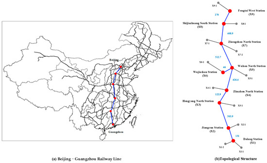
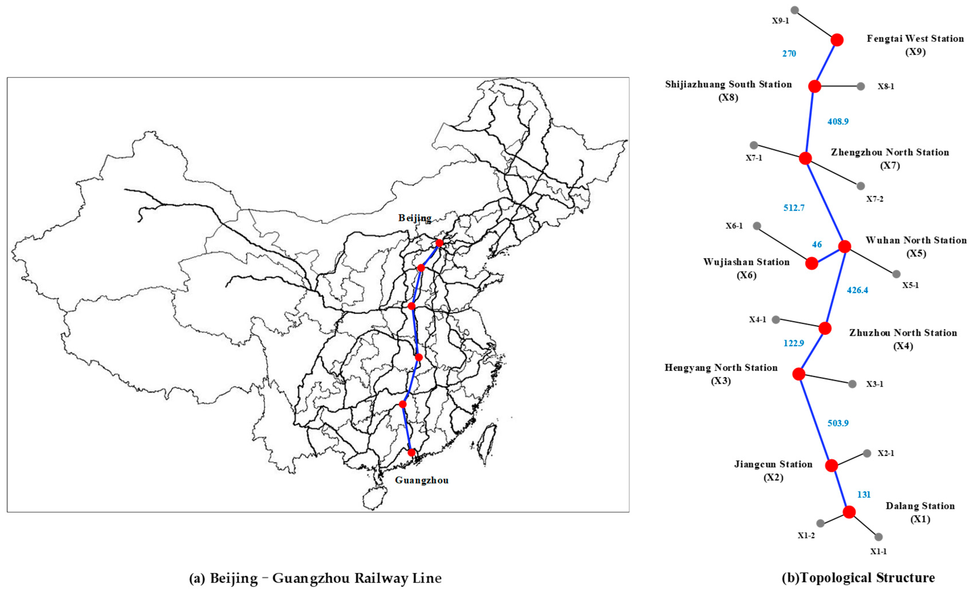
As one of the main north–south railroad lines and the major cargo transport corridors in China’s railroad network, “Beijing–Guangzhou Railway Line” starts from Beijing and reaches Guangzhou, spanning six provincial capitals or municipalities, with a total length of 2324 km. It has great significance in easing transport tension and strengthening economic and cultural exchanges, as shown in Figure 3a. This section selects seven important marshalling yards on the corridor, namely, Jiangcun Station, Hengyang North Station, Zhuzhou North Station, Wuhan North Station, Zhengzhou North Station, Shijiazhuang South Station, and Fengtai West Station, as well as two logistics hubs related to this corridor, Wujiashan Station and Dalang Station, as the hub nodes; the topological structure is shown in Figure 3b.

Figure 3. The topology of the road-rail intermodal network.

In this freight corridor, most of the cargo transported in the southward direction is bulk goods that are low-value, such as steel, coal, timber, cotton, cereals, etc., while among the cargo transported in the northward direction, the proportion of high-value goods is higher. Thus, this paper selects the northward shipments as the research object. The road terminals are directly connected to the rail hubs through road transport, as shown in Figure 3b. In addition, any road terminals can be connected by road transport. The blue numbers denote the length of rail physical arcs, in kilometres.

5.1. The Input Data

At present, there are three different grades of express train services in China, namely the normal express train, the fast express train, and the special express train, whose organisation mode is similar to that of passenger trains, having fixed departure and arrival stations, stopping stations, fixed train paths, and explicit frequency. While the ordinary trains are provided only between the two technical stations. As for road transport, it is carried out by trucks. The information on vehicles is shown in Table 1. The value of $\varpi$ is based on the data published on the website of China Railway 95306, and the value of $C^{\mathrm{Fix}}$ and $C^{\mathrm{Km}}$ are taken from 48.

Table 1. The information on vehicles.

Type of Vehicles	$\mathit{v}$	$\mathit{\varpi }$	${\mathit{C}}^{\mathbf{F}\mathbf{i}\mathbf{x}}$	${\mathit{C}}^{\mathbf{K}\mathbf{m}}$
Truck	25	0.3	1000	10
Ordinary train	60	0.086	9500	55
Normal express train	80	0.098	13000	85
Fast express train	120	0.103	17500	110
Special express train	160	0.140	25000	160

According to the generation rules of the train candidate set [48] and the actual transport situation, the ordinary train service is provided only between neighbouring marshalling yards, while the express train candidate set consists of eight trains. The information about the shipments is shown in Table 2. ‘$o_d$’ and ‘$d_d$’ represent the origin and destination of the shipment, respectively.

Table 2. The information on shipments.

Shipment	${\mathit{o}}_{\mathit{d}}$	${\mathit{d}}_{\mathit{d}}$	${\mathit{d}}_{\mathit{s}\mathit{t}}$	${\mathit{T}}_{\mathit{s}\mathit{t}}$	Shipment	${\mathit{o}}_{\mathit{d}}$	${\mathit{d}}_{\mathit{d}}$	${\mathit{d}}_{\mathit{s}\mathit{t}}$	${\mathit{T}}_{\mathit{s}\mathit{t}}$
Flow-01	X1-1	X2-1	365	24	Flow-28	X3-1	X5-1	320	32
Flow-02	X1-1	X3-1	480	34	Flow-29	X3-1	X6-1	300	36
Flow-03	X1-1	X4-1	440	46	Flow-30	X3-1	X7-1	360	58
Flow-04	X1-1	X5-1	500	60	Flow-31	X3-1	X7-2	340	56
Flow-05	X1-1	X6-1	540	64	Flow-32	X3-1	X8-1	290	70
Flow-06	X1-1	X7-1	460	46	Flow-33	X3-1	X9-1	310	70
Flow-07	X1-1	X7-2	620	54	Flow-34	X4-1	X5-1	290	40
Flow-08	X1-1	X8-1	580	58	Flow-35	X4-1	X6-1	300	34
Flow-09	X1-1	X9-1	650	92	Flow-36	X4-1	X7-1	320	52
Flow-10	X1-2	X2-1	290	20	Flow-37	X4-1	X7-2	310	46
Flow-11	X1-2	X3-1	370	36	Flow-38	X4-1	X8-1	290	64
Flow-12	X1-2	X4-1	420	42	Flow-39	X4-1	X9-1	330	64
Flow-13	X1-2	X5-1	510	52	Flow-40	X5-1	X6-1	470	36
Flow-14	X1-2	X6-1	490	64	Flow-41	X5-1	X7-1	510	40
Flow-15	X1-2	X7-1	480	54	Flow-42	X5-1	X7-2	460	40
Flow-16	X1-2	X7-2	570	52	Flow-43	X5-1	X8-1	420	50
Flow-17	X1-2	X8-1	600	66	Flow-44	X5-1	X9-1	500	66
Flow-18	X1-2	X9-1	590	72	Flow-45	X6-1	X7-1	440	32
Flow-19	X2-1	X3-1	430	36	Flow-46	X6-1	X7-2	380	46
Flow-20	X2-1	X4-1	540	44	Flow-47	X6-1	X8-1	360	50
Flow-21	X2-1	X5-1	490	56	Flow-48	X6-1	X9-1	400	60
Flow-22	X2-1	X6-1	470	54	Flow-49	X7-1	X8-1	330	32
Flow-23	X2-1	X7-1	500	56	Flow-50	X7-1	X9-1	290	40
Flow-24	X2-1	X7-2	600	56	Flow-51	X7-2	X8-1	310	32
Flow-25	X2-1	X8-1	470	76	Flow-52	X7-2	X9-1	270	40
Flow-26	X2-1	X9-1	630	94	Flow-53	X8-1	X9-1	280	32
Flow-27	X3-1	X4-1	280	24

The distance information between nodes is given in Table 3 and Table 4; the data is obtained from Gao De Map.

Table 3. The information on the distance $l_s^i$.

	X1-1	X1-2	X2-1	X3-1	X4-1	X5-1	X6-1	X7-1	X7-2	X8-1	X9-1
X1	80	65	–	–	–	–	–	–	–	–	–
X2	–	–	70	–	–	–	–	–	–	–	–
X3	–	–	–	90	–	–	–	–	–	–	–
X4	–	–	–	–	85	–	–	–	–	–	–
X5	–	–	–	–	–	100	–	–	–	–	–
X6	–	–	–	–	–	–	120	–	–	–	–
X7	–	–	–	–	–	–	–	90	105	–	–
X8	–	–	–	–	–	–	–	–	–	85	–
X9	–	–	–	–	–	–	–	–	–	–	90

Table 4. The information on the distance $l_s^t$.

	X1-1	X1-2	X2-1	X3-1	X4-1	X5-1	X6-1	X7-1	X7-2	X8-1	X9-1
X1-1	–	–	236	647	802	1114	1202	1618	1638	1958	2285
X1-2	–	–	171	582	737	1049	1137	1553	1574	1888	2215
X2-1	–	–	–	683	643	1190	1028	1594	1634	1924	2123
X3-1	–	–	–	–	299	531	589	955	996	1365	1765
X4-1	–	–	–	–	–	580	418	1020	1050	1375	1499
X5-1	–	–	–	–	–	–	242	520	540	914	1284
X6-1	–	–	–	–	–	–	–	668	708	1035	1163
X7-1	–	–	–	–	–	–	–	–	–	447	857
X7-2	–	–	–	–	–	–	–	–	–	397	842
X8-1	–	–	–	–	–	–	–	–	–	–	460
X9-1	–	–	–	–	–	–	–	–	–	–	–

As for the value of other parameters, the conversion coefficient of the original operating capacity $\theta$ is set to 0.85, and the average static load for $D^{\mathrm{Truck}}$ and $P$ are set to 37.5 tons per car and 50 tons per railcar, respectively. Additionally, the average number of marshalling railcars, denoted as $m_{ij}$, is 50 railcars, as well as the average transfer time for $\tau$ and ${\tau }_i$ are both established at 8 h [49].

5.2. Freight Strategy Analysis Based on Model RRIND

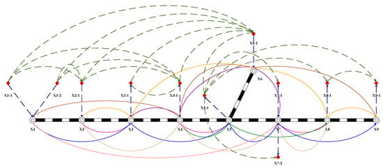
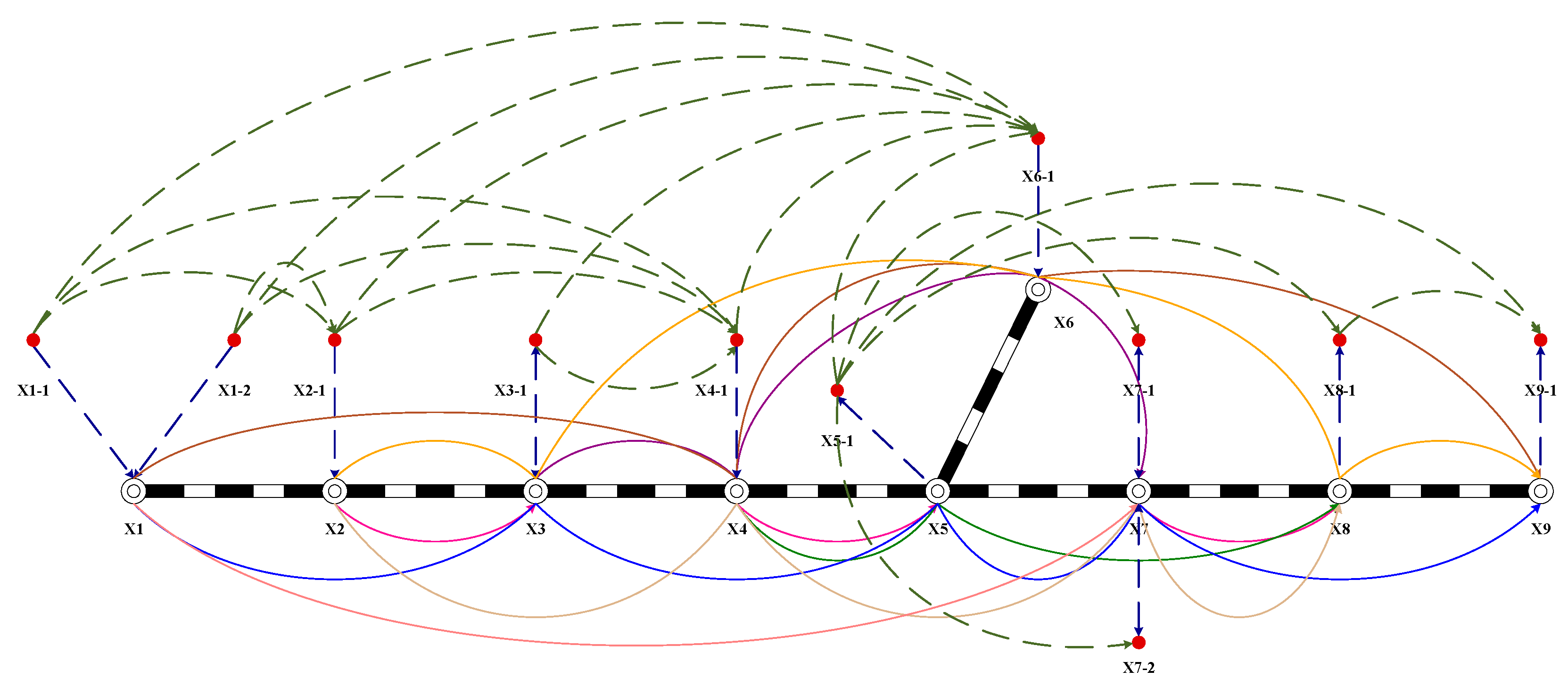
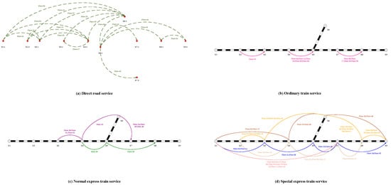
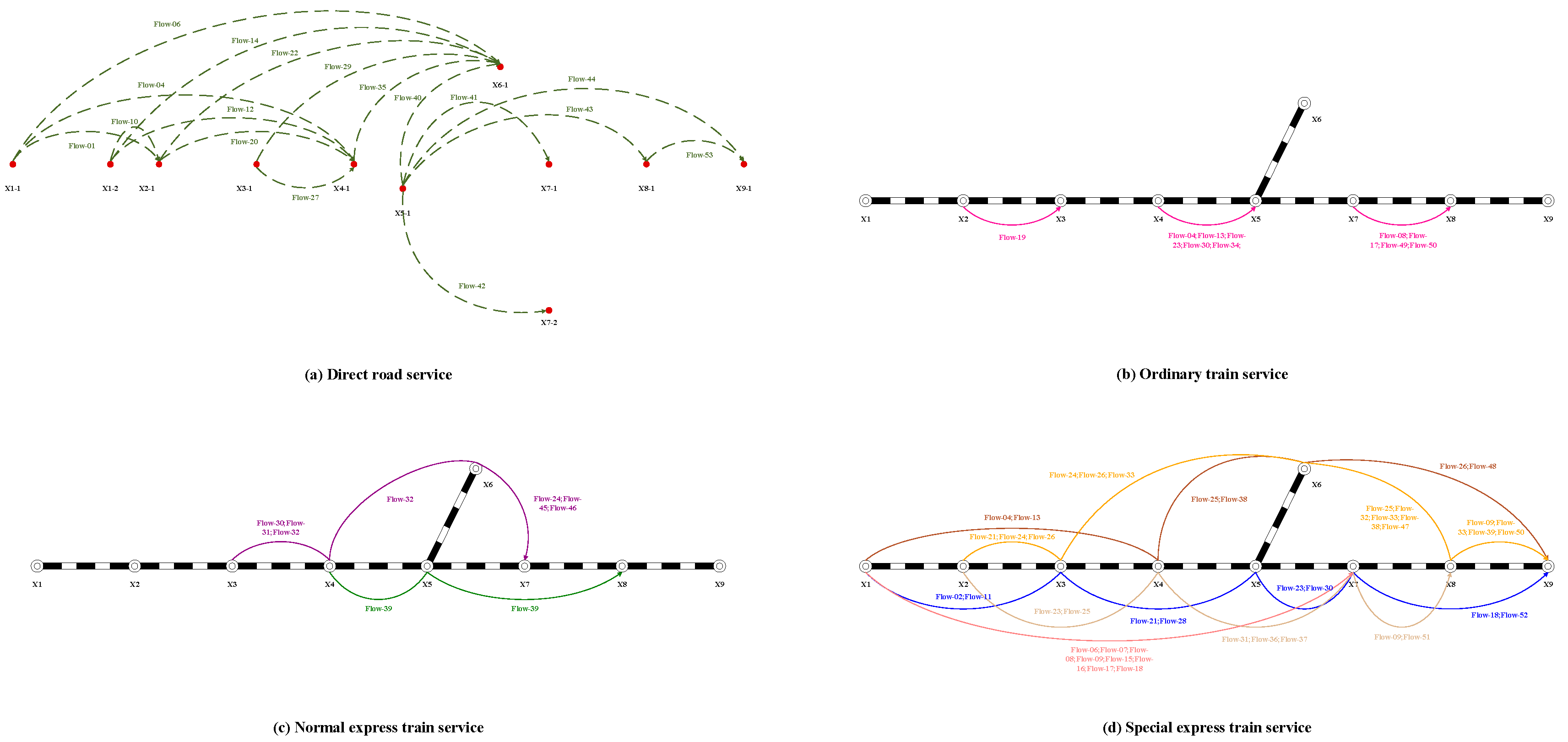
The current numerical experiments are conducted on a small-scale network due to the limited availability of reliable large-scale data. The model RRIND is solved by the commercial solver GUROBI 10.00 implemented in Python 3.7.7, and the optimal solution is obtained after running for 204.11 s when the Gap with the optimal objective value is 0.00%. The result shows that the maximum freight profit is 800,415.96 CNY, and freight services are provided as shown in Figure 4. The solid arcs of different colours in Figure 4 represent different rail freight services, while the olive drab dashed arcs represent direct road services, and the dark blue dashed arcs represent road feeder services. The deep pink solid arcs denote the ordinary train services, with the formulation plan of X2 → X3 (A), X4 → X5 (B), and X7 → X8 (C). Similarly, the purple solid arcs and the green solid arcs mean the normal express train services, with the operation plan of X3 → X4 → X6 → X7 (D) and X4 → X5 → X8 (E). Also, the blue solid arcs, the tan solid arcs, the sienna solid arcs, the orange solid arcs, and the light coral solid arc mean the special express train services, with the operation plan of X1 → X3 → X5 → X7 → X9 (F), X2 → X4 → X7 → X8 (G), X1 → X4 → X6 → X9 (H), X2 → X3 → X6 → X8 → X9 (I), and X1 → X7 (J). The values of service frequencies are detailed in Table 5.

Figure 4. The freight services.

Table 5. The frequency of each service.

Type of Services	Specific Service	Frequency
Ordinary train service	X2 → X3	1
	X4 → X5	1
	X7 → X8	1
Normal express train service	X3 → X4 → X6 → X7	1
	X4 → X5 → X8	1
Special express train service	X1 → X3 → X5 → X7 → X9	1
	X2 → X4 → X7 → X8	1
	X1 → X4 → X6 → X9	1
	X2 → X3 → X6 → X8 → X9	1
	X1 → X7	2
Direct road service	X1-1 → X2-1	10
	X1-1 → X4-1	12
	X1-1 → X6-1	15
	X1-2 → X2-1	8
	X1-2 → X4-1	12
	X1-2 → X6-1	14
	X2-1 → X4-1	15
	X2-1 → X6-1	13
	X3-1 → X4-1	8
	X3-1 → X6-1	8
	X4-1 → X6-1	8
	X5-1 → X6-1	13
	X5-1 → X7-1	14
	X5-1 → X7-2	13
	X5-1 → X8-1	12
	X5-1 → X9-1	14
	X8-1 → X9-1	8

The assignment plan of shipments is shown in Table 6.

Table 6. The assignment plan of shipments.

Shipment	${\mathit{T}}_{\mathit{s}\mathit{t}}$	${{\mathit{T}}_{\mathit{s}\mathit{t}}}^{\prime }$	Assignment Plan	Transport Mode
Flow-01	24	9.44	X1-1 → X2-1	Road service
Flow-02	34	26.77	X1-1 → X1 → X3 → X3-1	Road-rail service
Flow-03	46	32.08	X1-1 → X4-1	Road service
Flow-04	60	43.05	X1-1 → X1 → X4 → X5 → X5-1	Road-rail service
Flow-05	64	48.08	X1-1 → X6-1	Road service
Flow-06	46	35.12	X1-1 → X1 → X7 → X7-1	Road-rail service
Flow-07	54	35.72	X1-1 → X1 → X7 → X7-2	Road-rail service
Flow-08	58	49.73	X1-1 → X1 → X7 → X8 → X8-1	Road-rail service
Flow-09	92	55.36	X1-1 → X1 → X7 → X8 → X9 → X9-1	Road-rail service
Flow-10	20	6.84	X1-2 → X2-1	Road service
Flow-11	36	26.17	X1-2 → X1 → X3 → X3-1	Road-rail service
Flow-12	42	29.48	X1-2 → X4-1	Road service
Flow-13	52	42.45	X1-2 → X1 → X4 → X5 → X5-1	Road-rail service
Flow-14	64	45.48	X1-2 → X6-1	Road service
Flow-15	54	34.52	X1-2 → X1 → X7 → X7-1	Road-rail service
Flow-16	52	35.12	X1-2 → X1 → X7 → X7-2	Road-rail service
Flow-17	66	49.13	X1-2 → X1 → X7 → X8 → X8-1	Road-rail service
Flow-18	72	46.76	X1-2 → X1 → X7 → X9 → X9-1	Road-rail service
Flow-19	36	30.78	X2-1 → X2 → X3 → X3-1	Road-rail service
Flow-20	44	25.72	X2-1 → X4-1	Road service
Flow-21	56	37.39	X2-1 → X2 → X3 → X5 → X5-1	Road-rail service
Flow-22	54	41.12	X2-1 → X6-1	Road service
Flow-23	56	52.63	X2-1 → X2 → X4 → X5 → X7 → X7-1	Road-rail service
Flow-24	56	52.86	X2-1 → X2 → X3 → X6 → X7 → X7-2	Road-rail service
Flow-25	76	51.12	X2-1 → X2 → X4 → X6 → X8 → X8-1	Road-rail service
Flow-26	94	53.01	X2-1 → X2 → X3 → X6 → X9 → X9-1	Road-rail service
Flow-27	24	11.96	X3-1 → X4-1	Road service
Flow-28	32	27.04	X3-1 → X3 → X5 → X5-1	Road-rail service
Flow-29	36	23.56	X3-1 → X6-1	Road service
Flow-30	58	51.05	X3-1 → X3 → X4 → X5 → X7 → X7-1	Road-rail service
Flow-31	56	39.21	X3-1 → X3 → X4 → X7 → X7-2	Road-rail service
Flow-32	70	52.49	X3-1 → X3 → X4 → X6 → X8 → X8-1	Road-rail service
Flow-33	70	50.66	X3-1 → X3 → X6 → X8 → X9 → X9-1	Road-rail service
Flow-34	40	30.51	X4-1 → X4 → X5 → X5-1	Road-rail service
Flow-35	34	16.72	X4-1 → X6-1	Road service
Flow-36	52	28.87	X4-1 → X4 → X7 → X7-1	Road-rail service
Flow-37	46	29.47	X4-1 → X4 → X7 → X7-2	Road-rail service
Flow-38	64	39.80	X4-1 → X4 → X6 → X8 → X8-1	Road-rail service
Flow-39	64	50.80	X4-1 → X4 → X5 → X8 → X9 → X9-1	Road-rail service
Flow-40	36	9.68	X5-1 → X6-1	Road service
Flow-41	40	20.80	X5-1 → X7-1	Road service
Flow-42	40	21.60	X5-1 → X7-2	Road service
Flow-43	50	36.56	X5-1 → X8-1	Road service
Flow-44	66	51.36	X5-1 → X9-1	Road service
Flow-45	32	31.39	X6-1 → X6 → X7 → X7-1	Road-rail service
Flow-46	46	31.99	X6-1 → X6 → X7 → X7-2	Road-rail service
Flow-47	50	30.25	X6-1 → X6 → X8 → X8-1	Road-rail service
Flow-48	60	32.14	X6-1 → X6 → X9 → X9-1	Road-rail service
Flow-49	32	29.82	X7-1 → X7 → X8 → X8-1	Road-rail service
Flow-50	40	39.71	X7-1 → X7 → X8 → X9 → X9-1	Road-rail service
Flow-51	32	26.16	X7-2 → X7 → X8 → X8-1	Road-rail service
Flow-52	40	28.05	X7-2 → X7 → X9 → X9-1	Road-rail service
Flow-53	32	18.40	X8-1 → X9-1	Road service

${T_{st}}^{\prime }$ represents the actual transport time, and it can be found that all cargoes can be delivered to the destination before the transport due date $T_{st}$. Among these, 17 shipments are transported via direct road transport, as highlighted in bold in Table 6; the remaining shipments select the road-rail intermodal transport to complete their itinerary.

Figure 5a–d illustrate the shipments carried by direct road service and each of the freight train service arcs, respectively. As shown in Figure 5, the special express train service arc $\mathrm{X}1\to \mathrm{X}7$ (J1) carries the most shipments, eight in total, Flow-06-Flow-09 and Flow-15-Flow-18.

Figure 5. The shipments carried by the service arc.

The information on hubs is listed in Table 7. ${ℝ}_i$ means the actual workload of the rail hub, and ${\rho }_i$ refers to the utilisation of operating capacity. As can be seen in Table 7, X7 has the highest capacity utilisation, 85.84%, whereas X9 has the least capacity utilisation, 54.44%. The logistics hub X6 is handling an excessively saturated workload compared to the marshalling yard X5; therefore, it may be advisable to transfer some of the express train services currently routed through X6 to X5.

Table 7. The workload of hubs.

$\mathit{i}$	$\mathit{C}{\mathit{R}}_{{\mathit{i}}^{\prime }}$	$\mathit{C}{\mathit{L}}_{{\mathit{i}}^{″}}$	$\mathit{\theta }$	${\mathsf{ℝ}}_{\mathit{i}}$	${\mathit{\rho }}_{\mathit{i}}$
X1	–	200	0.85	6410	75.42%
X2	100	–	0.85	3120	73.42%
X3	180	–	0.85	4620	60.40%
X4	150	–	0.85	4510	70.75%
X5	120	–	0.85	2940	57.65%
X6	–	120	0.85	4170	81.77%
X7	250	–	0.85	9120	85.84%
X8	150	–	0.85	4810	75.46%
X9	150	–	0.85	3470	54.44%

5.3. Freight Strategy Analysis Based on Model RRIND_C1

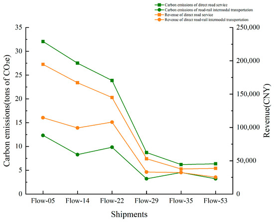
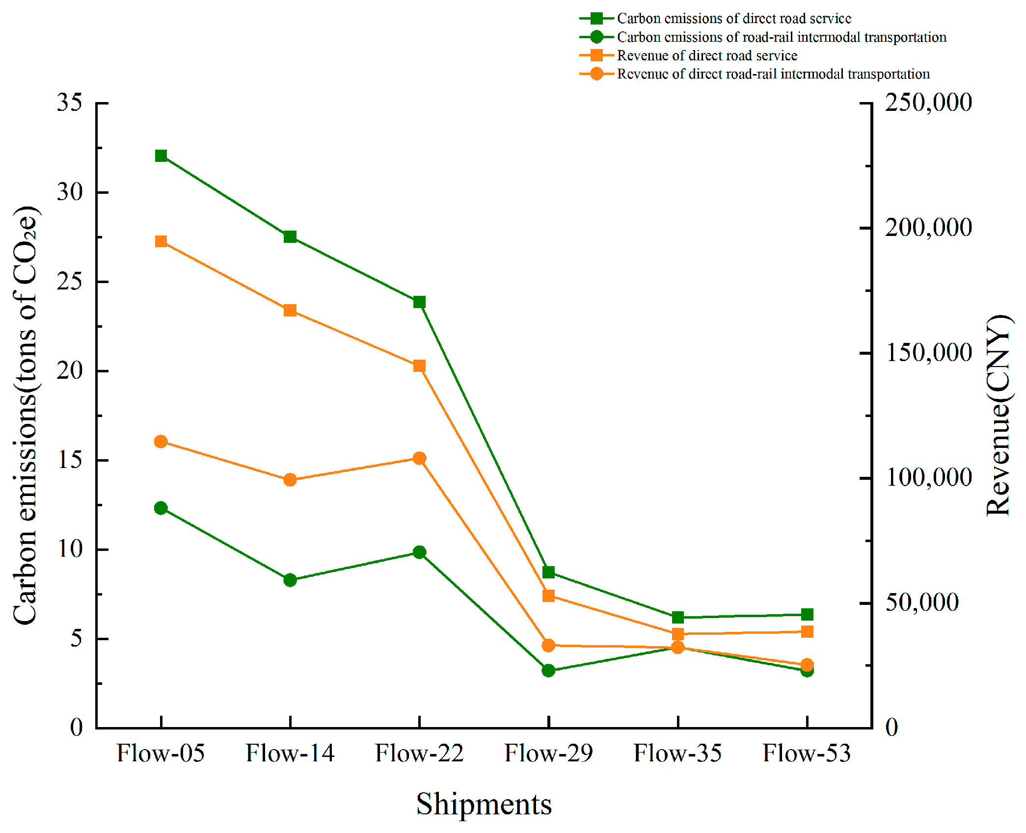
The parameters ${\zeta }^{\mathrm{Rail}}$ and ${\zeta }^{\mathrm{Road}}$ are set to 0.1053 × 10⁻⁴ and 0.494 × 10⁻⁴ tons of CO₂e per tonne–kilometre, respectively [50]. The carbon emission allowance $E^{\mathrm{Carbon}}$ is equal to 600 tons of CO₂e. The model RRIND_C1 yields an optimal objective value of 798,360.82 CNY, which is slightly lower than the optimal result of the model RRIND. The result demonstrates that Flow-05, Flow-14, Flow-22, Flow-29, Flow-35, and Flow-53 are all changed from direct road service to road-rail intermodal transport under CAC. The changes in carbon emissions and revenue for the six shipments mentioned above are quantitatively demonstrated in Figure 6, revealing emission intensity differentials before and after CAC.

Figure 6. Carbon emissions of shipments.

When $E^{\mathrm{Carbon}}$ is 550 tons of CO₂e, the optimal result shows that the objective value is 765,472.01 CNY, and Flow-03, Flow-05, Flow-12, Flow-14, Flow-20, Flow-22, Flow-27, Flow-29 and Flow-35 are all converted to road-rail intermodal transport. When $E^{\mathrm{Carbon}}$ is 500 tons of CO₂e, the model is infeasible, and there is no optimal solution, which may be due to the conflict between the carbon emission allowance constraint and the transport due date constraint.

5.4. Freight Strategy Analysis Based on Model RRIND_C2

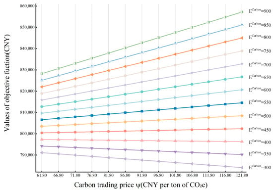
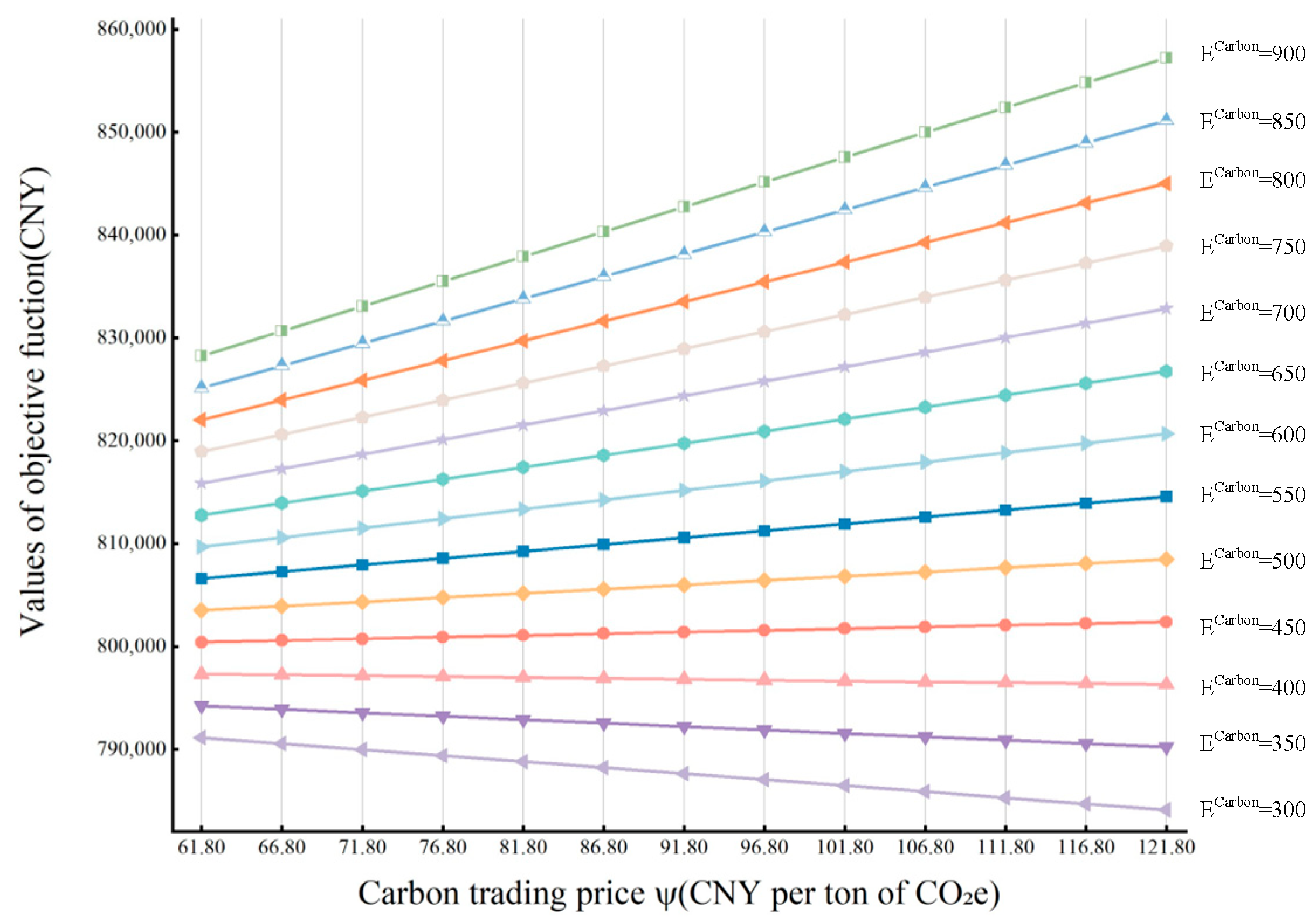
The parameter $\psi$ is set to 91.80 CNY per tonne of CO₂e [51], and the optimal objective value of model RRIND_C2 is 815,173.30 CNY, which is slightly higher than that of model RRIND. This profit variation may be attributed to two principal factors: One is the modal shift in partial shipments (i.e., Flow-05, Flow-14, Flow-22, Flow-29, Flow-35, and Flow-53) from direct road transport to road-rail intermodal transport, which reduces freight rates while simultaneously decreasing associated operational costs. Additionally, the allocated carbon emission allowance $E^{\mathrm{Carbon}}$ has a potential surplus, which can generate additional revenue through carbon trading markets. Figure 7 demonstrates the objective function values under different combinations of $E^{\mathrm{Carbon}}$ and $\psi$.

Figure 7. Objective function values with different $E^{\mathrm{Carbon}}$ and $\psi$.

The effect of the value of $E^{\mathrm{Carbon}}$ and $\psi$ on the objective function can be visualised from Figure 7. When the value of $E^{\mathrm{Carbon}}$ is equal to 300, 350, and 400 tons of CO₂e, the objective function decreases gradually with the increase of $\psi$, whereas when $E^{\mathrm{Carbon}}$ is greater than 400 tons of CO₂e, the objective function increases as $\psi$ increases. These observations confirm that both carbon emission allowance and carbon trading price significantly influence the optimisation of road-rail intermodal networks. This linear trend is theoretically expected because the carbon trading price enters the objective function linearly, while the emission level remains constant within each optimal solution regime, leading to a piecewise linear response. In actual production, enterprises should comprehensively consider the dynamic interactions between carbon emission allowance and market-driven carbon price during the planning period to achieve optimal economic-environmental coordination.

5.5. Freight Strategy Analysis Based on Model RRIND_C3

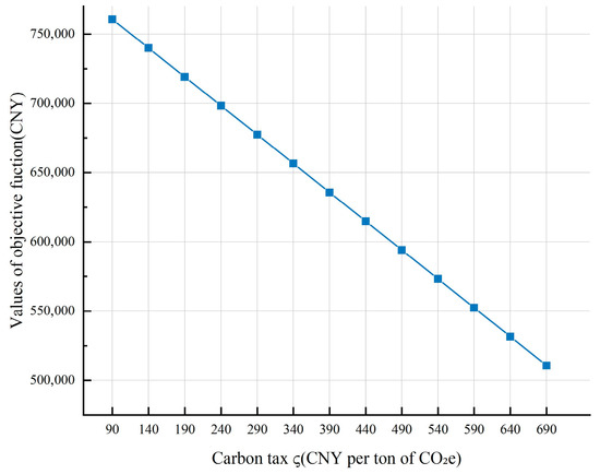
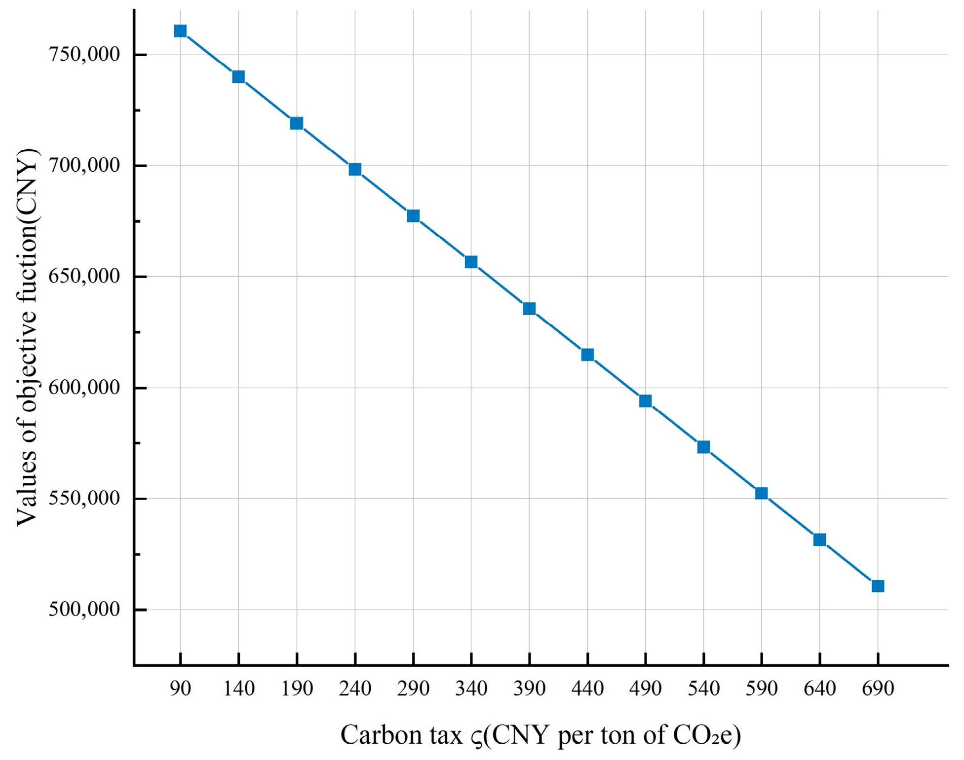
Since China has not yet implemented the carbon tax policy, the value of $\varsigma$ is established to be 90 CNY per tonne of CO₂e [52] by referencing the tax rates of China’s Environmental Protection Tax (EPT) and international carbon tax practices. The RRIND_C3 yields an optimal objective value of 760,843.65 CNY, which is lower than the optimal result of the model RRIND. The result shows that Flow-05, Flow-14, Flow-22, Flow-29, Flow-35, and Flow-53 are converted to road-rail intermodal transport. We calculate the values of the objective function with different $\varsigma$; the result is shown in Figure 8.

Figure 8. Objective function values with different $\varsigma$.

Figure 8 demonstrates a significant negative correlation between the objective function value and the carbon tax, which may be due to the transport due date constraint that restricts transport mode selection. Some shipments can only choose direct road transport with higher carbon emissions under the arrival period constraints, even though the carbon tax is increasing. This trend is theoretically consistent with the structure of the objective function. Since the carbon tax term enters the model as a linear penalty proportional to total carbon emissions, the objective value varies linearly with the carbon tax rate when the optimal transport plan remains unchanged. Furthermore, excessively high carbon tax rates may lead to suboptimal corporate profitability margins, potentially resulting in operational deficits. Consequently, policymakers should holistically consider both corporate financial viability and emission reduction targets when formulating carbon taxation frameworks. It is imperative to implement dynamic adjustment mechanisms coupled with phased tax incentives, thereby establishing a balanced policy architecture that reconciles environmental objectives with economic sustainability.

6. Conclusions

In this paper, we investigated the road-rail intermodal network design problem under carbon emission policies. First, we introduced three common carbon emission policies, i.e., CAC, ETS, and carbon tax. Then, a novel 0-1 nonlinear model was presented with profit maximisation as the objective function, which can satisfy transport due date restrictions. In addition, the linearisation techniques were introduced to reduce the complexity of the model. And, the extended models under three carbon emission policies were developed. Finally, a numerical example was constructed to test the model, and the sensitivity analysis of carbon emission-related parameters was conducted.

The result indicates that the final decision is heavily influenced by carbon emission policies, specifically, different allocated carbon emission allowances, carbon trading prices, and carbon tax rates lead to significant differences in optimisation results. These pivotal parameters work together to determine the final operational schemes. The findings demonstrate that incorporating carbon emission policies into intermodal service network design is essential for achieving coordinated economic and environmental performance under increasingly stringent emission reduction targets.

It should be noted that the applicability of the proposed model is subject to specific operational conditions. The framework is primarily designed for short-term planning scenarios in which transport demand, infrastructure configuration, and carbon price levels can be treated as deterministic within the planning horizon. The decision-making perspective corresponds to a profit-oriented carrier operating on an existing road-rail network. Under such settings, the model provides a structured tool for evaluating operational adjustments under alternative carbon emission policies.

Several limitations should also be acknowledged. First, carbon price uncertainty and market dynamics are not considered, as the model assumes a stable carbon price within the planning horizon. Second, potential behavioural adjustments, such as demand elasticity or route choices beyond the predefined service set, are not incorporated. Third, although the exact linearisation preserves the optimal solution of the original formulation, large-scale national applications may require advanced decomposition or heuristic solution approaches to enhance computational efficiency.

Note that with the introduction of carbon peak and carbon neutrality targets, and given the limitations of single-policy instruments in reducing emissions, transport enterprises are unlikely to face a single carbon regulation environment in the future. Instead, operational decisions may be affected by synergistic interactions among diverse carbon emission policies. Accordingly, future research should further explore the interaction mechanisms among multiple carbon policy instruments within the road-rail intermodal network design framework, as well as investigate dynamic and stochastic extensions to enhance the model’s practical applicability.

References

- Assad, A.A. Models for rail transportation. Transp. Res. Part A Gen. 1980, 14, 205–220. [Google Scholar] [CrossRef] [Scilit]
- Wang, Z.; Qi, M.; Cheng, C.; Zhang, C. A hybrid algorithm for large-scale service network design considering a heterogeneous fleet. Eur. J. Oper. Res. 2019, 276, 483–494. [Google Scholar] [CrossRef] [Scilit]
- Friesz, T.L.; Tobin, R.L.; Harker, P.T. Predictive intercity freight network models: The state of the art. Transp. Res. Part A Gen. 1983, 17, 409–417. [Google Scholar] [CrossRef] [Scilit]
- Crainic, T.G. Service network design in freight transportation. Eur. J. Oper. Res. 2000, 122, 272–288. [Google Scholar] [CrossRef] [Scilit]
- Wieberneit, N. Service network design for freight transportation: A review. OR Spectr. 2008, 30, 77–112. [Google Scholar] [CrossRef] [Scilit]
- Pedersen, M.B.; Crainic, T.G.; Madsen, O.B. Models and tabu search metaheuristics for service network design with asset-balance requirements. Transp. Sci. 2009, 43, 158–177. [Google Scholar] [CrossRef] [Scilit]
- Balakrishnan, A.; Magnanti, T.L.; Wong, R.T. A dual-ascent procedure for large-scale uncapacitated network design. Oper. Res. 1989, 37, 716–740. [Google Scholar] [CrossRef] [Scilit]
- Holmberg, K.; Hellstrand, J. Solving the uncapacitated network design problem by a Lagrangean heuristic and branch-and-bound. Oper. Res. 1998, 46, 247–259. [Google Scholar] [CrossRef] [Scilit]
- Lamar, B.W.; Sheffi, Y.; Powell, W.B. A capacity improvement lower bound for fixed charge network design problems. Oper. Res. 1990, 38, 704–710. [Google Scholar] [CrossRef] [Scilit]
- Holmberg, K.; Yuan, D. A Lagrangian heuristic based branch-and-bound approach for the capacitated network design problem. Oper. Res. 2000, 48, 461–481. [Google Scholar] [CrossRef] [Scilit]
- Kalantari, N.; Mirzahossein, H.; Najafi, P.; Waller, T.; Zhang, X. Continuous network design using partial linearized subgradient methods. Transp. Res. Rec. 2023, 2677, 633–643. [Google Scholar] [CrossRef] [Scilit]
- Mirzahossein, H.; Najafi, P.; Kalantari, N.; Waller, T. Solving discrete network design problem using disjunctive constraints. Comput. Aided Civ. Infrastruct. Eng. 2025, 40, 1028–1042. [Google Scholar] [CrossRef] [Scilit]
- Crainic, T.G.; Rousseau, J.M. Multicommodity, multimode freight transportation: A general modeling and algorithmic framework for the service network design problem. Transp. Res. Part B Methodol. 1986, 20, 225–242. [Google Scholar] [CrossRef] [Scilit]
- Kim, D.; Barnhart, C. Transportation service network design: Models and algorithms. In Computer-Aided Transit Scheduling: Proceedings, Cambridge, MA, USA, August 1997; Springer: Berlin/Heidelberg, Germany, 1999; pp. 259–283. [Google Scholar] [CrossRef] [Scilit]
- Crainic, T.G.; Hewitt, M.; Toulouse, M.; Vu, D.M. Service network design with resource constraints. Transp. Sci. 2016, 50, 1380–1393. [Google Scholar] [CrossRef] [Scilit]
- Andersen, J.; Crainic, T.G.; Christiansen, M. Service network design with asset management: Formulations and comparative analyses. Transp. Res. Part C Emerg. Technol. 2009, 17, 197–207. [Google Scholar] [CrossRef] [Scilit]
- Li, X.; Ding, Y.; Pan, K.; Jiang, D.; Aneja, Y.P. Single-path service network design problem with resource constraints. Transp. Res. Part E Logist. Transp. Rev. 2020, 140, 101945. [Google Scholar] [CrossRef] [Scilit]
- Jiang, X.; Bai, R.; Atkin, J.; Kendall, G. A scheme for determining vehicle routes based on Arc-based service network design. INFOR Inf. Syst. Oper. Res. 2017, 55, 16–37. [Google Scholar] [CrossRef] [Scilit]
- Teypaz, N.; Schrenk, S.; Cung, V.D. A decomposition scheme for large-scale service network design with asset management. Transp. Res. Part E Logist. Transp. Rev. 2010, 46, 156–170. [Google Scholar] [CrossRef] [Scilit]
- Li, X.; Wei, K.; Aneja, Y.P.; Tian, P. Design-balanced capacitated multicommodity network design with heterogeneous assets. Omega 2017, 67, 145–159. [Google Scholar] [CrossRef] [Scilit]
- Scherr, Y.O.; Saavedra, B.A.N.; Hewitt, M.; Mattfeld, D.C. Service network design with mixed autonomous fleets. Transp. Res. Part E Logist. Transp. Rev. 2019, 124, 40–55. [Google Scholar] [CrossRef] [Scilit]
- Barnhart, C.; Jin, H.; Vance, P.H. Railroad blocking: A network design application. Oper. Res. 2000, 48, 603–614. [Google Scholar] [CrossRef] [Scilit]
- Lulli, G.; Pietropaoli, U.; Ricciardi, N. Service network design for freight railway transportation: The Italian case. J. Oper. Res. Soc. 2011, 62, 2107–2119. [Google Scholar] [CrossRef] [Scilit]
- Zhu, E.; Crainic, T.G.; Gendreau, M. Scheduled service network design for freight rail transportation. Oper. Res. 2014, 62, 383–400. [Google Scholar] [CrossRef] [Scilit]
- López-Ramos, F.; Codina, E.; Marín, Á.; Guarnaschelli, A. Integrated approach to network design and frequency setting problem in railway rapid transit systems. Comput. Oper. Res. 2017, 80, 128–146. [Google Scholar] [CrossRef] [Scilit]
- Jarrah, A.I.; Johnson, E.; Neubert, L.C. Large-scale, less-than-truckload service network design. Oper. Res. 2009, 57, 609–625. [Google Scholar] [CrossRef] [Scilit]
- Grimault, A.; Bostel, N.; Lehuédé, F. An adaptive large neighborhood search for the full truckload pickup and delivery problem with resource synchronization. Comput. Oper. Res. 2017, 88, 1–14. [Google Scholar] [CrossRef] [Scilit]
- Farvolden, J.M.; Powell, W.B. Subgradient methods for the service network design problem. Transp. Sci. 1994, 28, 256–272. [Google Scholar] [CrossRef] [Scilit]
- Sung, C.S.; Song, S.H. Integrated service network design for a cross-docking supply chain network. J. Oper. Res. Soc. 2003, 54, 1283–1295. [Google Scholar] [CrossRef] [Scilit]
- Lium, A.G.; Crainic, T.G.; Wallace, S.W. A study of demand stochasticity in service network design. Transp. Sci. 2009, 43, 144–157. [Google Scholar] [CrossRef] [Scilit]
- Bai, R.; Wallace, S.W.; Li, J.; Chong, A.Y.L. Stochastic service network design with rerouting. Transp. Res. Part B Methodol. 2014, 60, 50–65. [Google Scholar] [CrossRef] [Scilit]
- Van Hui, Y.; Gao, J.; Leung, L.; Wallace, S. Airfreight forwarder’s shipment planning under uncertainty: A two-stage stochastic programming approach. Transp. Res. Part E Logist. Transp. Rev. 2014, 66, 83–102. [Google Scholar] [CrossRef] [Scilit]
- Yu, S.; Yang, Z.; Yu, B. Air express network design based on express path choices–Chinese case study. J. Air Transp. Manag. 2017, 61, 73–80. [Google Scholar] [CrossRef] [Scilit]
- Lai, M.F.; Lo, H.K. Ferry service network design: Optimal fleet size, routing, and scheduling. Transp. Res. Part A Policy Pract. 2004, 38, 305–328. [Google Scholar] [CrossRef] [Scilit]
- Lo, H.K.; An, K.; Lin, W.H. Ferry service network design under demand uncertainty. Transp. Res. Part E Logist. Transp. Rev. 2013, 59, 48–70. [Google Scholar] [CrossRef] [Scilit]
- Yang, D.; Pan, K.; Wang, S. On service network improvement for shipping lines under the one belt one road initiative of China. Transp. Res. Part E Logist. Transp. Rev. 2018, 117, 82–95. [Google Scholar] [CrossRef] [Scilit]
- Reinhardt, L.B.; Pisinger, D.; Sigurd, M.M.; Ahmt, J. Speed optimisations for liner networks with business constraints. Eur. J. Oper. Res. 2020, 285, 1127–1140. [Google Scholar] [CrossRef] [Scilit]
- Meng, Q.; Wang, S. Liner shipping service network design with empty container repositioning. Transp. Res. Part E Logist. Transp. Rev. 2011, 47, 695–708. [Google Scholar] [CrossRef] [Scilit]
- Kim, D.; Barnhart, C.; Ware, K.; Reinhardt, G. Multimodal express package delivery: A service network design application. Transp. Sci. 1999, 33, 391–407. [Google Scholar] [CrossRef] [Scilit]
- Riessen, B.V.; Negenborn, R.R.; Dekker, R.; Lodewijks, G. Service network design for an intermodal container network with flexible transit times and the possibility of using subcontracted transport. Int. J. Shipp. Transp. Logist. 2015, 7, 457–478. [Google Scholar] [CrossRef] [Scilit]
- Farahani, N.Z.; Noble, J.S.; McGarvey, R.G.; Enayati, M. An advanced intermodal service network model for a practical transition to synchromodal transport in the US Freight System: A case study. Multimodal Transp. 2023, 2, 100051. [Google Scholar] [CrossRef] [Scilit]
- Laaziz, E.H.; Sbihi, N. A service network design model for an intermodal rail-road freight forwarder. Int. J. Logist. Syst. Manag. 2019, 32, 465–482. [Google Scholar] [CrossRef] [Scilit]
- Demir, E.; Burgholzer, W.; Hrušovský, M.; Arıkan, E.; Jammernegg, W.; Van Woensel, T. A green intermodal service network design problem with travel time uncertainty. Transp. Res. Part B Methodol. 2016, 93, 789–807. [Google Scholar] [CrossRef] [Scilit]
- Uddin, M.; Huynh, N. Reliable routing of road-rail intermodal freight under uncertainty. Netw. Spat. Econ. 2019, 19, 929–952. [Google Scholar] [CrossRef] [Scilit]
- Bouchery, Y.; Fransoo, J. Cost, carbon emissions and modal shift in intermodal network design decisions. Int. J. Prod. Econ. 2015, 164, 388–399. [Google Scholar] [CrossRef] [Scilit]
- Inghels, D.; Dullaert, W.; Vigo, D. A service network design model for multimodal municipal solid waste transport. Eur. J. Oper. Res. 2016, 254, 68–79. [Google Scholar] [CrossRef] [Scilit]
- Lam, J.S.L.; Gu, Y. A market-oriented approach for intermodal network optimisation meeting cost, time and environmental requirements. Int. J. Prod. Econ. 2016, 171, 266–274. [Google Scholar] [CrossRef] [Scilit]
- Meng, Y.; Lin, B. Integrated optimisation of railway freight service: Express trains and ordinary trains. Int. J. Syst. Sci. Oper. Logist. 2025, 12, 2436654. [Google Scholar] [CrossRef] [Scilit]
- Lin, B.; Duan, J.; Wang, J.; Sun, M.; Peng, W.; Liu, C.; Xiao, J.; Liu, S.; Wu, J. A study of the car-to-train assignment problem for rail express cargos in the scheduled and unscheduled train services network. PLoS ONE 2018, 13, e0204598. [Google Scholar] [CrossRef] [Scilit] [PubMed]
- Lin, B.; Liu, C.; Wang, H.; Lin, R. Modeling the railway network design problem: A novel approach to considering carbon emissions reduction. Transp. Res. Part D Transp. Environ. 2017, 56, 95–109. [Google Scholar] [CrossRef] [Scilit]
- Wang, K.; Lyu, C. Review and outlook of global and China carbon markets. J. Beijing Inst. Technol. 2025, 27, 19–36. [Google Scholar] [CrossRef]
- Cui, Z.; Wang, S.; Zu, Q. On the design of the Chinese carbon tax system in the context of implementation of EU carbon tariffs. Tax. Res. 2024, 11, 50–54. [Google Scholar] [CrossRef]
Disclaimer/Publisher’s Note: The statements, opinions and data contained in all publications are solely those of the individual author(s) and contributor(s) and not of MDPI and/or the editor(s). MDPI and/or the editor(s) disclaim responsibility for any injury to people or property resulting from any ideas, methods, instructions or products referred to in the content. |
© 2026 by the authors. Licensee MDPI, Basel, Switzerland. This article is an open access article distributed under the terms and conditions of the Creative Commons Attribution (CC BY) license.