Construction of a New Discrete Chaotic Mapping Based on the Robust Chaos Theorem

Abstract

Chaotic systems serve as fundamental pseudo-random sequence generators in encryption algorithms and play a vital role in communication security. However, most current research still focus on the classical Logistic chaotic map, making it vulnerable to targeted attacks. To address this issue, this paper proposes a general construction method for a class of cubic chaotic maps over the real number field and proves the existence of chaos based on the robust chaos criterion for S-unimodal maps. Furthermore, by integrating the proposed cubic chaotic map with the infinite folding map, a new one-dimensional discrete chaotic map is developed. Dynamical analysis demonstrates that, compared with the infinite folding map and the Logistic map, the newly constructed map exhibits stronger chaotic behavior and more stable complexity, showing superior potential for practical applications in secure communications.

1. Introduction

Discrete chaotic mappings constitute a class of mathematical models that have been extensively studied in dynamical systems and chaos theory, and they are capable of effectively characterizing the nonlinear dynamical behavior of a wide range of natural and social systems. Among them, the Logistic map has been widely adopted in various chaotic cryptosystems due to its high computational efficiency and simple, easily controllable parameter structure. In 1976, the famous biologist May proposed the Logistic mathematical model [1]. The proposal of logistic mappings can be said to be the beginning of the study of discrete chaotic systems, which is important for the development of discrete chaotic systems. After that, many discrete chaotic systems were proposed, such as the familiar Tent mapping [2] and Cubic mapping [3]. The study of discrete chaotic mappings is not only important for theoretical science, but also has a wide range of applications. For example, it has important applications in communication encryption [4], image encryption [5,6,7,8,9], chaotic cryptanalysis [10,11], and communication security [12,13]. Therefore, the in-depth study of discrete chaotic mappings has important theoretical and practical significance.

Kocarev et al. [14] pointed out that, in the design of chaotic ciphers, the selected chaotic map should at least possess three essential properties: strong mixing property, robustness, and a large parameter space. The mixing property requires that any slight variation in the plaintext be sufficiently diffused to affect as many ciphertext components as possible. Robustness refers to the ability of a chaotic system to preserve its chaotic behavior under small parameter perturbations, thereby ensuring its inherent space-diffusion characteristics. Therefore, when constructing a chaos-based cryptographic algorithm, it is highly desirable to select chaotic systems that exhibit both strong mixing and robustness over a wide range of parameter values. Song et al. [15] proposed a composite chaotic system (S-L-F) with cascaded sinusoidal mapping, generalized third-order Fibonacci, and logistic chaos. Alawida et al. [16] enhanced the dynamical structure of the classical logistic map, significantly enlarging its chaotic parameter range and improving randomness and robustness for cryptographic applications. Subsequently, Hosny et al. [17] proposed a multi-image encryption framework integrating multiple chaotic maps, which effectively strengthens diffusion, key sensitivity, and resistance to cryptanalytic attacks. In addition, Fedoseev et al. [18] introduced a discrete chaotic map with adaptive symmetry for encryption design, further improving dynamical complexity and overall security performance. These studies indicate that chaotic maps exhibiting strong mixing and robustness over wide parameter ranges remain crucial for the design of secure chaos-based cryptographic algorithms.

In recent years, with the advancement of chaotic control and reinforcement learning technologies, robustness analysis of chaotic systems has attracted considerable research interest. Several studies have focused on modeling and dynamical analysis of chaotic systems, including detailed investigations of high-dimensional and hyperchaotic dynamics and adaptive synchronization behaviors [19,20,21,22]. Concurrently, efforts have been made in the control and optimization of chaotic systems, where novel control strategies such as reinforcement learning-based control and adaptive active set methods are introduced to enhance stability and robustness under perturbations [23,24,25,26]. These approaches, including complex nonlinear feedback and adaptive reliability optimization, systematically improve the stability, performance, and robustness of chaotic behavior under varying parameter and information conditions. For example, based on previous results, Xu et al. [27] proposed a general method for a class of quadratic chaotic mappings and justified its existence based on a robust chaos determination theorem for S single-peaked mappings. In addition, several studies have leveraged the intrinsic properties of chaotic systems to develop optimization algorithms, such as particle swarm optimization and ant colony optimization [28]. Consequently, enhancing the intrinsic characteristics of chaotic systems—particularly improving their robustness from a theoretical perspective—remains of critical importance. Chaotic robustness is a complex and fundamental issue, with broad applications in chaotic control, system optimization, and secure information processing. This paper proposes a general method for constructing cubic chaotic mappings based on the robust chaos theorem, which further improves the robustness of chaotic systems and provides better methods and ideas for solving practical problems. Finally, based on the proposed construction method, a cubic chaotic map was generated and then combined with the infinite folding map to yield a novel discrete chaotic map. Dynamical analysis confirms that this new map exhibits stronger chaotic properties than both the infinite folding map and the Logistic map.

The rest of the paper is organized as follows: in Section 2, the parameter settings of a general class of cubic chaotic mappings are given based on the S-peak mapping theorem, and the results are verified by data simulation experiments. In Section 3, a more complex discrete chaotic mapping is constructed based on the robust chaos theorem given in Section 2, combined with an infinite folding mapping, and its dynamics is analyzed.

2. Robust Chaos for General Cubic Mapping

Based on Li-York’s “period three implies chaos” theorem, Andrecut and Ali proposed a judgment theorem [29] for robust chaos of S single-peaked mappings.

Definition 1.

Mapping $\phi \left(x\right)$: $J=\left[p,q\right]\to J$ is called $S$ single-peaked mapping if the following conditions are satisfied.

(1)

The mapping $\phi \left(x\right)$ has a continuous third-order derivative function;

(2)

$p$ is an immovable point, and there exists an original image $q$, i.e., $\phi \left(p\right)=\phi \left(q\right)=p$;

(3)

The existence of a unique maximal point $m$ on the interval $\left[p,q\right]$ for the mapping $\phi \left(x\right)$ such that the mapping $\phi \left(x\right)$ strictly increases on the interval $\left[p,m\right)$ and strictly decreases on the interval $\left(m,q\right]$;

(4)

Mapping $\phi \left(x\right)$ has a negative Schwarzian derivatives, i.e.,

$$S\left(\phi ,x\right)={\displaystyle \frac{{\phi }^{‴}\left(x\right)}{{\phi }_{\prime }\left(x\right)}}-{\displaystyle \frac{3{({\phi }^{″}\left(x\right))}^2}{2{({\phi }^{\prime }\left(x\right))}^2}}<0.$$

(1)

The chaos theorem based on the S single-peaked mapping is as follows.

Theorem 1.

If the mapping ${\phi }_v\left(x\right)$: $J=\left[p,q\right]\to J$ is a $S$ single-peaked mapping containing the parameters $v$ and there exists a maximum at the point $m\in \left(p,q\right)$ such that for any parameter$v\in \left(v_{min},v_{max}\right)$, ${\phi }_v\left(m\right)=q$, then the mapping ${\phi }_v\left(x\right)$ for any parameter $v\in \left(v_{min},v_{max}\right)$ is chaotic.

Here, the cubic formula and its proof are given below.

Theorem 2.

Given a general cubic equation with real coefficients $a{x}^3+b{x}^2+cx+d=0$, let $D=b^2-3ac$ ($\lambda \in R$); if $D>0$, $\left|\lambda \right|<1$, set $\lambda =\cos \theta$ $(0<\theta <\pi )$, then the equation has three unequal real roots

$$\left\{\begin{array}{l}{x}_1={\displaystyle \frac{-b+\sqrt{D}\cdot 2\cos (\frac{\theta }{3})}{3a}},\hfill \\ x_2={\displaystyle \frac{-b+\sqrt{D}\cdot 2\cos (\frac{\theta }{3}+\frac{2}{3}\pi )}{3a}},\hfill \\ x_3={\displaystyle \frac{-b+\sqrt{D}\cdot 2\cos (\frac{\theta }{3}-\frac{2}{3}\pi )}{3a}}.\hfill \end{array}\right.$$

(2)

where $\theta ={\cos }^{-1}\lambda$.

Corollary 1.

The general cubic equation with real coefficients $a{x}^3+b{x}^2+cx+d=0$ has three unequal real roots, then

(a)

If $a>0$, then $x_2<x_3<x_1$;

(b)

If $a<0$, then $x_1<x_3<x_2$.

The judgment theorem for robust chaos of general cubic polynomial mapping is constructed below.

Let the cubic function be

$$\phi \left(x\right)=a{x}^3+b{x}^2+cx+d,\left(a\ne 0\right)$$

(3)

where let $D=b^2-3ac$, $\lambda ={\displaystyle \frac{9abc-2b^3-27a^{2}d}{2{(\sqrt{D})}^3}}$. Let the parameters $v\in \left(-\infty ,0\right)\cup (4,$$+\infty )$, such that $b^2=vac$; to construct the chaotic mapping, it is first obvious that there exists a continuous third-order derivative of $\phi \left(x\right)$:

$${\phi }^{\prime }\left(x\right)=3a{x}^2+2bx+c,$$

(4)

$${\phi }^{″}\left(x\right)=6ax+2b,$$

(5)

$${\phi }^{‴}\left(x\right)=6a.$$

(6)

Let ${\phi }^{\prime }\left(x\right)=0$, we can solve for $m={\displaystyle \frac{-b-\sqrt{D}}{3a}}$ and $m^{\ast }={\displaystyle \frac{-b+\sqrt{D}}{3a}}$, where $m$ and $m^{\ast }$ are the extreme value points of $\phi \left(x\right)$. Substituting $m$ and $m^{\ast }$ into Equation (5), we obtain

$${\phi }^{″}\left(m\right)=6a{\displaystyle \frac{-b-\sqrt{D}}{3a}}+2b=-2b-2\sqrt{D}+2b=-2\sqrt{D}<0$$

(7)

$${\phi }^{″}\left(m^{\ast }\right)=6a{\displaystyle \frac{-b+\sqrt{D}}{3a}}+2b=-2b+2\sqrt{D}+2b=2\sqrt{D}>0$$

(8)

So $m$ is the local maximum point of $\phi \left(x\right)$, and $m^{\ast }$ is the local minimum point of $\phi \left(x\right)$.

For $\forall a,b,c,d\in R$, all have

$$\begin{array}{ll}S(\phi ,x)& ={\displaystyle \frac{{\phi }^{‴}(x)}{{\phi }^{\prime }(x)}}-{\displaystyle \frac{3{({\phi }^{″}(x))}^2}{2{({\phi }^{\prime }(x))}^2}}\\ & ={\displaystyle \frac{6a}{3a{x}^2+2bx+c}}-{\displaystyle \frac{3{(6ax+2b)}^2}{2{(3a{x}^2+2bx+c)}^2}}\\ & ={\displaystyle \frac{12a(3a{x}^2+2bx+c)-3{(6ax+2b)}^2}{2{(3a{x}^2+2bx+c)}^2}}\\ & =-6{\displaystyle \frac{6a^2{x}^2+4abx-ac+b^2}{2{(3a{x}^2+2bx+c)}^2}}\\ & =-6{\displaystyle \frac{6{(ax+\frac{b}{3})}^2+\frac{(b^2-3ac)}{3}}{2{(3a{x}^2+2bx+c)}^2}}<0.\end{array}$$

(9)

Therefore, $\phi \left(x\right)$ has a negative Schwarzian derivative.

To consider all cases of the coefficient sign, a discussion of the case is needed.

1. When $a>0$,

(1)

If $b>0$, assume that in $\phi \left(x\right)$ there exists three unequal real roots, and by Theorem 2, there must be $D>0,$$\left|\lambda \right|<1$, and $\forall v\in \left(-\infty ,0\right)\cup \left(4,+\infty \right)$. There must be $\sqrt{b^2-4ac}>\sqrt{D}=$$\sqrt{b^2-3ac}>0$ and therefore $D>0$.

Let $\left|\lambda \right|<1$, that is, $-1<{\displaystyle \frac{9abc-2b^3-27a^{2}d}{2{(\sqrt{D})}^3}}<1$. Because $2{(\sqrt{D})}^3>0$, $-2{(\sqrt{D})}^3<$$9abc-2b^3-27a^{2}d<2{(\sqrt{D})}^3,$ $9abc-2b^3-2{(\sqrt{D})}^3<27a^{2}d.$

Set $27a^{2}d=u(9abc-2b^3+2(\sqrt{D}{)}^3),$ and have ${\displaystyle \frac{9abc-2b^3-2{(\sqrt{D})}^3}{9abc-2b^3+2{(\sqrt{D})}^3}}<u<1.$ Because $v={\displaystyle \frac{b^2}{ac}}$, $\sqrt{D}=\sqrt{b^2-3ac}$; there are ${\displaystyle \frac{\frac{9}{v} -2-2{(\sqrt{1-\frac{3}{v}})}^3}{\frac{9}{v} -2+2{(\sqrt{1-\frac{3}{v}})}^3}}<u<1$, that is,

$$1-{\displaystyle \frac{4{(1-\frac{3}{v})}^{\frac{3}{2}}}{\frac{9}{v}-2+2{(1-\frac{3}{v})}^{\frac{3}{2}}}}<u<1$$

(10)

and by assumption that $27a^{2}d=u(9abc-2b^3+2(\sqrt{D}{)}^3)$, there are

$$\begin{array}{ll}\lambda & ={\displaystyle \frac{9abc-2b^3-27a^{2}d}{2{(\sqrt{D})}^3}}\\ & ={\displaystyle \frac{9abc-2b^3-u(9abc-2b^3+2{(\sqrt{D})}^3)}{2{(\sqrt{D})}^3}}\\ & ={\displaystyle \frac{9-2v-9u+2uv}{2v{(1-\frac{3}{v})}^{\frac{3}{2}}}}-u.\end{array}$$

(11)

From $\lambda =\cos \theta (0<\theta <\pi )$, we have

$$\theta ={\cos }^{-1}\lambda ={\cos }^{-1}({\displaystyle \frac{9-2v-9u+2uv}{2v{(1-\frac{3}{v})}^{\frac{3}{2}}}}-u)$$

(12)

From Theorem 2, we can solve for $\phi \left(x\right)=0$ with three unequal real roots:

$$\left\{\begin{array}{l}{x}_1={\displaystyle \frac{-b+\sqrt{D}\cdot 2\cos (\frac{\theta }{3})}{3a}},\hfill \\ x_2={\displaystyle \frac{-b+\sqrt{D}\cdot 2\cos (\frac{\theta }{3}+\frac{2}{3}\pi )}{3a}},\hfill \\ x_3={\displaystyle \frac{-b+\sqrt{D}\cdot 2\cos (\frac{\theta }{3}-\frac{2}{3}\pi )}{3a}}.\hfill \end{array}\right.$$

(13)

By Corollary 1, when $a>0$, the roots of $\phi \left(x\right)=0$ are $x_1>x_3>x_2$, and because $m<m^{\ast }$, let $p=x_2,q=x_3,r=x_1$, so the function $\phi \left(x\right)$ is increasing on $\left(p,m\right)$ and decreasing on $\left(m,q\right)$ and $\phi \left(p\right)=\phi \left(q\right)=0$.

Let there be another cubic function:

$${\phi }^{\ast }\left(x\right)=a{x}^3+b{x}^2+cx+d^{\ast }. \left(a\ne 0\right)$$

(14)

where $d^{\ast }=d+p={\displaystyle \frac{u\left(9abc-2b^3+2{(\sqrt{D})}^3\right)-9ab+2\sqrt{D}\cos (\frac{\theta }{3}+\frac{2}{3}\pi )}{27a^2}}$, then there must be $\phi \left(p\right)=\phi \left(q\right)=p$. Then, at this time, the function ${\phi }^{\ast }\left(x\right)$ is $S$ single-peaked mapping.

To make ${\phi }^{\ast }\left(x\right)$ a chaotic mapping,

$$\begin{array}{ll}{{\phi }^{\ast }}_{u,v}(m)& =a{({\displaystyle \frac{-b-\sqrt{D}}{3a}})}^3+b{({\displaystyle \frac{-b-\sqrt{D}}{3a}})}^2+c({\displaystyle \frac{-b-\sqrt{D}}{3a}})+d^{\ast }\\ & ={\displaystyle \frac{-b^3-3b^2\sqrt{D}-3bD-{(\sqrt{D})}^3}{27a^2}}+{\displaystyle \frac{b^3+2b^2\sqrt{D}+D}{9a^2}}+{\displaystyle \frac{-bc-c\sqrt{D}}{3a}}+d^{\ast }.\end{array}$$

(15)

Substituting $D=b^2-3ac$, let ${{\phi }^{\ast }}_{u,v}\left(m\right)=q$; then we have

$$\begin{array}{ll}{{\phi }^{\ast }}_{u,v}(m)& ={\displaystyle \frac{2b^3+3b^2\sqrt{b^2-3ac}-9abc-{(\sqrt{b^2-3ac})}^3-9ac\sqrt{b^2-3ac}+27a^2{d}^{\ast }}{27a^2}}\\ & ={\displaystyle \frac{(2-2u)b^3+(3b^2-9ac)\sqrt{b^2-3ac}-(9u-9)abc-{(\sqrt{b^2-3ac})}^3+2u{(\sqrt{b^2-3ac})}^3}{27a^2}}\\ & -{\displaystyle \frac{9ab-18a\sqrt{b^2-3ac}\cos (\frac{\theta }{3}+\frac{2}{3}\pi )}{27a^2}}\\ & ={\displaystyle \frac{-9ab+18a\sqrt{b^2-3ac}\cos (\frac{\theta }{3}-\frac{2}{3}\pi )}{27a^2}},\end{array}$$

(16)

$$\begin{array}{l}{\displaystyle \frac{\left(2-2u\right)b^3+\left(3b^2-9ac\right)\sqrt{b^2-3ac}-\left(9u-9\right)abc-{(\sqrt{b^2-3ac})}^3+2u{(\sqrt{b^2-3ac})}^3}{27a^2}}\\ ={\displaystyle \frac{18a\sqrt{b^2-3ac}\cos (\frac{\theta }{3}-\frac{2}{3}\pi )-18a\sqrt{b^2-3ac}\cos (\frac{\theta }{3}+\frac{2}{3}\pi )}{27a^2}}\end{array}$$

(17)

Then, from $b^2=vac$, we obtain

$$\begin{array}{c}\left(2-2u\right)b^3+b^3\left(3-{\displaystyle \frac{9}{v}}\right)\sqrt{b^2-3ac}-{\displaystyle \frac{\left(9u-9\right)}{v}}{b}^3-b^3{(1-{\displaystyle \frac{3}{v}})}^{\frac{3}{2}}+2u{b}^3{(1-{\displaystyle \frac{3}{v}})}^{\frac{3}{2}}\\ =18ab\sqrt{1-{\displaystyle \frac{3}{v}}}\left(\cos ({\displaystyle \frac{\theta }{3}}-{\displaystyle \frac{2}{3}}\pi )-\cos ({\displaystyle \frac{\theta }{3}}+{\displaystyle \frac{2}{3}}\pi )\right)\end{array}$$

(18)

Since $b>0$, it follows that

$$b=\sqrt{{\displaystyle \frac{18a\sqrt{1-\frac{3}{v}}\left(\cos (\frac{\theta }{3}-\frac{2}{3}\pi )-\cos (\frac{\theta }{3}+\frac{2}{3}\pi )\right)}{2-2u+\left(3-\frac{9}{v}\right)\sqrt{1-\frac{3}{v}}+\frac{\left(9u-9\right)}{v}+\left(2u-1\right){(1-\frac{3}{v})}^{\frac{3}{2}}}}},$$

(19)

$$d^{\ast }={\displaystyle \frac{9ab\left(uc-1\right)+18a\sqrt{b^2-3ac}\cos (\frac{\theta }{3}+\frac{2}{3}\pi )+2u{(b^2-3ac)}^{\frac{3}{2}}-2u{b}^3}{27a^2}}.$$

(20)

Then, if ${\phi }^{\ast }\left(m\right)$ parameters satisfy Equations (10), (12), (19) and (20), then ${\phi }^{\ast }\left(m\right)$ on the interval $\left[p,q\right]$ is chaotic.

To discuss other cases in the same way.

(2)

If $b<0$, assume that in $\phi \left(x\right)$ there exist three unequal real roots, and by Theorem 2, there must be $D>0$ and $\left|\lambda \right|<1$, and that $\forall v\in \left(-\infty ,0\right)\cup \left(4,+\infty \right)$. There must be $\sqrt{b^2-4ac}>$$D=\sqrt{b^2-3ac}>0$. Thus, $D>0$

By $b<0$, $\left|\lambda \right|<1$, it is observed that ${\displaystyle \frac{9abc-2b^3-2{(\sqrt{D})}^3}{9abc-2b^3+2{(\sqrt{D})}^3}}<u<1$, and because $v={\displaystyle \frac{b^2}{ac}}$, $\sqrt{D}=\sqrt{b^2-3ac}$, there are ${\displaystyle \frac{\frac{9}{v} -2+2{(\sqrt{1-\frac{3}{v}})}^3}{\frac{9}{v} -2-2{(\sqrt{1-\frac{3}{v}})}^3}}<u<1$, that is,

$$1+{\displaystyle \frac{4{(1-\frac{3}{v})}^{\frac{3}{2}}}{\frac{9}{v}-2-2{(1-\frac{3}{v})}^{\frac{3}{2}}}}<u<1.$$

(21)

Similarly, we can obtain

$$\begin{array}{ll}\theta & ={\cos }^{-1}({\displaystyle \frac{9abc-2b^3-u(9abc-2b^3+2{(\sqrt{D})}^3)}{2{(\sqrt{D})}^3}})\\ & ={\cos }^{-1}({\displaystyle \frac{9-2v-9u+2uv}{-2v{(1-\frac{3}{v})}^{\frac{3}{2}}}}-u)\end{array}$$

(22)

From (1), we still have $p={\displaystyle \frac{-b+\sqrt{D}\cdot 2\cos (\frac{\theta }{3}+\frac{2}{3}\pi )}{3a}},q={\displaystyle \frac{-b+\sqrt{D}\cdot 2\cos (\frac{\theta }{3}-\frac{2}{3}\pi )}{3a}}$. The function increases on $\left(p,m\right)$ and decreases on $\left(m,q\right)$ and $\phi \left(p\right)=\phi \left(q\right)=0$.

Therefore, from Equation (14), we have $\phi \left(p\right)=\phi \left(q\right)=p$. Then, the function ${\phi }^{\ast }\left(x\right)$ is $S$ single-peaked mapping at this time.

In order to make ${\phi }^{\ast }\left(x\right)$ a chaotic mapping, substitute $D=b^2-3ac$ into Equation (15), and let ${{\phi }^{\ast }}_{u,v}\left(m\right)=q$ to obtain

$$\begin{array}{ll}{{\phi }^{\ast }}_{u,v}(m)& ={\displaystyle \frac{2b^3+3b^2\sqrt{b^2-3ac}-9abc-{(\sqrt{b^2-3ac})}^3-9ac\sqrt{b^2-3ac}+27a^2{d}^{\ast }}{27a^2}}\\ & ={\displaystyle \frac{(2-2u)b^3+(3b^2-9ac)\sqrt{b^2-3ac}-(9u-9)abc-{(\sqrt{b^2-3ac})}^3+2u{(\sqrt{b^2-3ac})}^3}{27a^2}}\\ & -{\displaystyle \frac{9ab-18a\sqrt{b^2-3ac}\cos (\frac{\theta }{3}+\frac{2}{3}\pi )}{27a^2}}\\ & ={\displaystyle \frac{-9ab+18a\sqrt{b^2-3ac}\cos (\frac{\theta }{3}-\frac{2}{3}\pi )}{27a^2}},\end{array}$$

(23)

$$\begin{array}{l}{\displaystyle \frac{(2-2u)b^3}{27a^2}}+{\displaystyle \frac{(3b^2-9ac)\sqrt{b^2-3ac}}{27a^2}}-{\displaystyle \frac{(9u-9)abc}{27a^2}}-{\displaystyle \frac{{(\sqrt{b^2-3ac})}^3}{27a^2}}+{\displaystyle \frac{2u{(\sqrt{b^2-3ac})}^3}{27a^2}}\\ ={\displaystyle \frac{18a\sqrt{b^2-3ac}\cos (\frac{\theta }{3}-\frac{2}{3}\pi )}{27a^2}}-{\displaystyle \frac{18a\sqrt{b^2-3ac}\cos (\frac{\theta }{3}+\frac{2}{3}\pi )}{27a^2}}.\end{array}$$

(24)

Then, by $b^2=vac$, it follows that

$$\begin{array}{c}\left(2-2u\right)b^3+b^3\left(3-{\displaystyle \frac{9}{v}}\right)\sqrt{b^2-3ac}-{\displaystyle \frac{\left(9u-9\right)}{v}}{b}^3-b^3{(1-{\displaystyle \frac{3}{v}})}^{{\displaystyle \frac{3}{2}}}+2u{b}^3{(1-{\displaystyle \frac{3}{v}})}^{{\displaystyle \frac{3}{2}}}\\ =18ab\sqrt{1-{\displaystyle \frac{3}{v}}}\left(\cos ({\displaystyle \frac{\theta }{3}}-{\displaystyle \frac{2}{3}}\pi )-\cos ({\displaystyle \frac{\theta }{3}}+{\displaystyle \frac{2}{3}}\pi )\right).\end{array}$$

(25)

Since $b<0$, it follows that

$$b=-\sqrt{{\displaystyle \frac{18a\sqrt{1-\frac{3}{v}}\left(\cos (\frac{\theta }{3}+\frac{2}{3}\pi )-\cos (\frac{\theta }{3}-\frac{2}{3}\pi )\right)}{2-2u-\left(3-\frac{9}{v}\right)\sqrt{1-\frac{3}{v}}+\frac{\left(9u-9\right)}{v}+\left(2u-1\right){(1-\frac{3}{v})}^{\frac{3}{2}}}}}$$

(26)

$$d^{\ast }={\displaystyle \frac{9ab\left(uc-1\right)+18a\sqrt{b^2-3ac}\cos (\frac{\theta }{3}+\frac{2}{3}\pi )+2u{(b^2-3ac)}^{\frac{3}{2}}-2u{b}^3}{27a^2}}.$$

(27)

Then, if ${\phi }^{\ast }\left(m\right)$ parameters satisfy Equations (14)–(17), then ${\phi }^{\ast }\left(m\right)$ on the interval $\left[p,q\right]$ is chaotic.

2. When $a<0$,

(1)

If $b>0$, using the same method, at this time, the range of $u$ satisfies Equation (10) and $\theta$ satisfies Equation (12), i.e., $\theta ={\cos }^{-1}\lambda ={\cos }^{-1}({\displaystyle \frac{9-2v-9u+2uv}{2v{(1-\frac{3}{v})}^{\frac{3}{2}}}}-u)$.

Since $a<0$, it follows from the corollary that $x_1<x_3<x_2$ and $m>m^{\ast }$; let $p=x_3={\displaystyle \frac{-b+\sqrt{D}\cdot 2\cos (\frac{\theta }{3}-\frac{2}{3}\pi )}{3a}},q=x_2={\displaystyle \frac{-b+\sqrt{D}\cdot 2\cos (\frac{\theta }{3}+\frac{2}{3}\pi )}{3a}}$, so the function $\phi \left(x\right)$ is increasing on $\left(p,m\right)$ and decreasing on $\left(m,q\right)$, and $\phi \left(p\right)=\phi \left(q\right)=0$.

Let the cubic function

$${\phi }^{\ast }\left(x\right)=a{x}^3+b{x}^2+cx+d^{\ast }.\left(a\ne 0\right)$$

(28)

Among them, $d^{\ast }=d+p={\displaystyle \frac{u\left(9abc-2b^3+2{(\sqrt{D})}^3\right)-9ab+2\sqrt{D}\cos (\frac{\theta }{3}-\frac{2}{3}\pi )}{27a^2}}$. Then, there clearly is $\phi \left(p\right)=\phi \left(q\right)=p$. Then, at this point, the function ${\phi }^{\ast }\left(x\right)$ is $S$ single-peaked mapping.

In order to make ${\phi }^{\ast }\left(x\right)$ a chaotic mapping, we substitute $D=b^2-3ac$ into Equation (15) and let ${{\phi }^{\ast }}_{u,v}\left(m\right)=q$ to obtain

$$\begin{array}{ll}{{\phi }^{\ast }}_{u,v}(m)& ={\displaystyle \frac{2b^3+3b^2\sqrt{b^2-3ac}-9abc-{(\sqrt{b^2-3ac})}^3-9ac\sqrt{b^2-3ac}+27a^2{d}^{\ast }}{27a^2}}\\ & ={\displaystyle \frac{(2-2u)b^3+(3b^2-9ac)\sqrt{b^2-3ac}-(9u-9)abc-{(\sqrt{b^2-3ac})}^3}{27a^2}}\\ & +{\displaystyle \frac{2u{(\sqrt{b^2-3ac})}^3-9ab+18a\sqrt{b^2-3ac}\cos (\frac{\theta }{3}-\frac{2}{3}\pi )}{27a^2}}\\ & ={\displaystyle \frac{-9ab+18a\sqrt{b^2-3ac}\cos (\frac{\theta }{3}+\frac{2}{3}\pi )}{27a^2}},\end{array}$$

(29)

$$\begin{array}{l}{\displaystyle \frac{\left(2-2u\right)b^3+\left(3b^2-9ac\right)\sqrt{b^2-3ac}-\left(9u-9\right)abc-{(\sqrt{b^2-3ac})}^3+2u{(\sqrt{b^2-3ac})}^3}{27a^2}}\\ ={\displaystyle \frac{18a\sqrt{b^2-3ac}\cos (\frac{\theta }{3}+\frac{2}{3}\pi )}{27a^2}}-{\displaystyle \frac{18a\sqrt{b^2-3ac}\cos (\frac{\theta }{3}-\frac{2}{3}\pi )}{27a^2}}\end{array}$$

(30)

Then, by $b^2=vac$, it follows that

$$\begin{array}{l}\left(2-2u\right)b^3+b^3\left(3-{\displaystyle \frac{9}{v}}\right)\sqrt{b^2-3ac}-{\displaystyle \frac{\left(9u-9\right)}{v}}{b}^3-b^3{\left(1-{\displaystyle \frac{3}{v}}\right)}^{\frac{3}{2}}+2u{b}^3{\left(1-{\displaystyle \frac{3}{v}}\right)}^{\frac{3}{2}}\\ =18ab\sqrt{1-{\displaystyle \frac{3}{v}}}(\cos ({\displaystyle \frac{\theta }{3}}+{\displaystyle \frac{2}{3}}\pi )-\cos ({\displaystyle \frac{\theta }{3}}-{\displaystyle \frac{2}{3}}\pi )).\end{array}$$

(31)

Since $b>0$, it follows that

$$b=\sqrt{{\displaystyle \frac{18a\sqrt{1-\frac{3}{v}}\left(\cos (\frac{\theta }{3}+\frac{2}{3}\pi )-\cos (\frac{\theta }{3}-\frac{2}{3}\pi )\right)}{2-2u+\left(3-\frac{9}{v}\right)\sqrt{1-\frac{3}{v}}+\frac{\left(9u-9\right)}{v}+\left(2u-1\right){(1-\frac{3}{v})}^{\frac{3}{2}}}}},$$

(32)

$$d^{\ast }={\displaystyle \frac{9ab\left(uc-1\right)+18a\sqrt{b^2-3ac}\cos (\frac{\theta }{3}-\frac{2}{3}\pi )+2u{(b^2-3ac)}^{\frac{3}{2}}-2u{b}^3}{27a^2}}.$$

(33)

If the parameters of ${\phi }^{\ast }\left(m\right)$ satisfy Equations (10), (12), (32) and (33), then ${\phi }^{\ast }\left(m\right)$ is chaotic on the interval $\left[p,q\right]$.

(2)

If $b<0$, then the range of $u$ satisfies Equation (21), $\theta$ satisfies Equation (22), and ${\phi }^{\ast }\left(x\right)$ is $S$ single-peaked mapping.

In order to make ${\phi }^{\ast }\left(x\right)$ a chaotic mapping, we substitute $D=b^2-3ac$ into Equation (15) and let ${{\phi }^{\ast }}_{u,v}\left(m\right)=q$ to obtain

$$\begin{array}{ll}{{\phi }^{\ast }}_{u,v}(m)& ={\displaystyle \frac{2b^3+3b^2\sqrt{b^2-3ac}-9abc-{(\sqrt{b^2-3ac})}^3-9ac\sqrt{b^2-3ac}+27a^2{d}^{\ast }}{27a^2}}\\ & ={\displaystyle \frac{(2-2u)b^3+(3b^2-9ac)\sqrt{b^2-3ac}-(9u-9)abc-{(\sqrt{b^2-3ac})}^3}{27a^2}}\\ & +{\displaystyle \frac{2u{(\sqrt{b^2-3ac})}^3-9ab+18a\sqrt{b^2-3ac}\cos (\frac{\theta }{3}-\frac{2}{3}\pi )}{27a^2}}\\ & ={\displaystyle \frac{-9ab+18a\sqrt{b^2-3ac}\cos (\frac{\theta }{3}+\frac{2}{3}\pi )}{27a^2}},\end{array}$$

(34)

$$\begin{array}{l}{\displaystyle \frac{\left(2-2u\right)b^3+\left(3b^2-9ac\right)\sqrt{b^2-3ac}-\left(9u-9\right)abc-{(\sqrt{b^2-3ac})}^3+2u{(\sqrt{b^2-3ac})}^3}{27a^2}}\\ ={\displaystyle \frac{18a\sqrt{b^2-3ac}\cos (\frac{\theta }{3}+\frac{2}{3}\pi )-18a\sqrt{b^2-3ac}\cos (\frac{\theta }{3}-\frac{2}{3}\pi )}{27a^2}}\end{array}$$

(35)

Then, by $b^2=vac$, it follows that

$$\begin{array}{c}\left(2-2u\right)b^3+b^3\left(3-{\displaystyle \frac{9}{v}}\right)\sqrt{b^2-3ac}-{\displaystyle \frac{\left(9u-9\right)}{v}}{b}^3-b^3{(1-{\displaystyle \frac{3}{v}})}^{\frac{3}{2}}+2u{b}^3{(1-{\displaystyle \frac{3}{v}})}^{\frac{3}{2}}\\ =18ab\sqrt{1-{\displaystyle \frac{3}{v}}}\left(\cos ({\displaystyle \frac{\theta }{3}}+{\displaystyle \frac{2}{3}}\pi )-\cos ({\displaystyle \frac{\theta }{3}}-{\displaystyle \frac{2}{3}}\pi )\right).\end{array}$$

(36)

Since $b<0$, it follows that

$$b=-\sqrt{{\displaystyle \frac{18a\sqrt{1-\frac{3}{v}}\left(\cos (\frac{\theta }{3}-\frac{2}{3}\pi )-\cos (\frac{\theta }{3}+\frac{2}{3}\pi )\right)}{2-2u-\left(3-\frac{9}{v}\right)\sqrt{1-\frac{3}{v}}+\frac{\left(9u-9\right)}{v}-\left(2u-1\right){(1-\frac{3}{v})}^{\frac{3}{2}}}}},$$

(37)

$$d^{\ast }={\displaystyle \frac{9ab\left(uc-1\right)+18a\sqrt{b^2-3ac}\cos (\frac{\theta }{3}-\frac{2}{3}\pi )+2u{(b^2-3ac)}^{\frac{3}{2}}-2u{b}^3}{27a^2}}$$

(38)

If the parameters of ${\phi }^{\ast }\left(m\right)$ satisfy Equations (21), (22), (37) and (38), then ${\phi }^{\ast }\left(m\right)$ on the interval $\left[p,q\right]$ is chaotic.

As above, all sign cases of the parameters are considered, so that the cubic polynomial discrete chaos determination theorem can be given.

Theorem 3.

Let the cubic function be

$$\phi \left(x\right)=a{x}^3+b{x}^2+cx+d\left(a\ne 0\right).$$

(39)

Let  $b^2=vac$,  $v\in \left(-\infty ,0\right)\cup \left(3,+\infty \right)$, then  $\phi \left(x\right)$  is a chaotic mapping if the set of parameters  $S=\left\{a,u,v,d,\theta \right\}$  satisfies any of the following cases.

Condition (1): If  $a>0$,

Case (i)

$$\left\{\begin{array}{l}1-{\displaystyle \frac{4{(1-\frac{3}{v})}^{\frac{3}{2}}}{\frac{9}{v}-2+2{(1-\frac{3}{v})}^{\frac{3}{2}}}}\le u\le 1,\hfill \\ b=\sqrt{{\displaystyle \frac{18a\sqrt{1-\frac{3}{v}}\left(\cos (\frac{\theta }{3}-\frac{2}{3}\pi )-\cos (\frac{\theta }{3}+\frac{2}{3}\pi )\right)}{2-2u+\left(3-\frac{9}{v}\right)\sqrt{1-\frac{3}{v}}+\frac{\left(9u-9\right)}{v}+\left(2u-1\right){(1-\frac{3}{v})}^{\frac{3}{2}}}}},\hfill \\ d={\displaystyle \frac{9ab\left(uc-1\right)+18a\sqrt{b^2-3ac}\cos (\frac{\theta }{3}+\frac{2}{3}\pi )+2u{(b^2-3ac)}^{\frac{3}{2}}-2u{b}^3}{27a^2}},\hfill \\ \theta ={\cos }^{-1}({\displaystyle \frac{9-2v-9u+2uv}{2v{(1-\frac{3}{v })}^{\frac{3}{2}}}}-u).\hfill \end{array}\right.$$

(40)

Case (ii)

$$\left\{\begin{array}{l}1+{\displaystyle \frac{4{(1-\frac{3}{v})}^{\frac{3}{2}}}{\frac{9}{v}-2-2{(1-\frac{3}{v})}^{\frac{3}{2}}}}\le u\le 1,\hfill \\ b=-\sqrt{{\displaystyle \frac{18a\sqrt{1-\frac{3}{v}}\left(\cos (\frac{\theta }{3}+\frac{2}{3}\pi )-\cos (\frac{\theta }{3}-\frac{2}{3}\pi )\right)}{2-2u-\left(3-\frac{9}{v}\right)\sqrt{1-\frac{3}{v}}+\frac{\left(9u-9\right)}{v}-\left(2u-1\right){(1-\frac{3}{v})}^{\frac{3}{2}}}}},\hfill \\ d={\displaystyle \frac{9ab\left(uc-1\right)+18a\sqrt{b^2-3ac}\cos (\frac{\theta }{3}+\frac{2}{3}\pi )+2u{(b^2-3ac)}^{\frac{3}{2}}-2u{b}^3}{27a^2}},\hfill \\ \theta ={\cos }^{-1}({\displaystyle \frac{9-2v-9u+2uv}{-2v{(1-\frac{3}{v})}^{\frac{3}{2}}}}-u).\hfill \end{array}\right.$$

(41)

Then, $\phi \left(x\right):$ $J=\left[p,q\right]\to J$ is a single-peaked mapping, where $p=-{\displaystyle \frac{b}{3a}}+$${\displaystyle \frac{2\sqrt{b^2-3ac}\cos (\frac{\theta }{3}+\frac{2}{3}\pi )}{3a}}$, $q={\displaystyle \frac{-b+2\sqrt{b^2-3ac}\cos (\frac{\theta }{3}-\frac{2}{3}\pi )}{3a}}$, and there exists a point $m={\displaystyle \frac{-b-\sqrt{b^2-3ac}}{3a}}\in \left[p,q\right]$ such that $\phi \left(m\right)=q$.

Condition (2): If $a<0$,

Case (i)

$$\left\{\begin{array}{l}1-{\displaystyle \frac{4{(1-\frac{3}{v})}^{\frac{3}{2}}}{\frac{9}{v}-2+2{(1-\frac{3}{v})}^{\frac{3}{2}}}}\le u\le 1,\hfill \\ b=\sqrt{{\displaystyle \frac{18a\sqrt{1-\frac{3}{v}}\left[\cos (\frac{\theta }{3}+\frac{2}{3}\pi )-\cos (\frac{\theta }{3}-\frac{2}{3}\pi )\right]}{2-2u+\left(3-\frac{9}{v}\right)\sqrt{1-\frac{3}{v}}+\frac{\left(9u-9\right)}{v}+\left(2u-1\right){(1-\frac{3}{v})}^{\frac{3}{2}}}}},\hfill \\ d={\displaystyle \frac{9ab\left(uc-1\right)+18a\sqrt{b^2-3ac}\cos (\frac{\theta }{3}-\frac{2}{3}\pi )+2u{(b^2-3ac)}^{\frac{3}{2}}-2u{b}^3}{27a^2}},\hfill \\ \theta ={\cos }^{-1}({\displaystyle \frac{9-2v-9u+2uv}{2v{(1-\frac{3}{v})}^{\frac{3}{2}}}}-u).\hfill \end{array}\right.$$

(42)

Case (ii)

$$\left\{\begin{array}{l}1+{\displaystyle \frac{4{(1-\frac{3}{v})}^{\frac{3}{2}}}{\frac{9}{v}-2-2{(1-\frac{3}{v})}^{\frac{3}{2}}}}\le u\le 1,\hfill \\ b=-\sqrt{{\displaystyle \frac{18a\sqrt{1-\frac{3}{v}}\left[\cos (\frac{\theta }{3}-\frac{2}{3}\pi )-\cos (\frac{\theta }{3}+\frac{2}{3}\pi )\right]}{2-2u-\left(3-\frac{9}{v}\right)\sqrt{1-\frac{3}{v}}+\frac{\left(9u-9\right)}{v}-\left(2u-1\right){(1-\frac{3}{v})}^{\frac{3}{2}}}}},\hfill \\ d={\displaystyle \frac{9ab\left(uc-1\right)+18a\sqrt{b^2-3ac}\cos (\frac{\theta }{3}-\frac{2}{3}\pi )+2u{(b^2-3ac)}^{\frac{3}{2}}-2u{b}^3}{27a^2}},\hfill \\ \theta ={\cos }^{-1}({\displaystyle \frac{9-2v-9u+2uv}{-2v{(1-\frac{3}{v})}^{\frac{3}{2}}}}-u).\hfill \end{array}\right.$$

(43)

Then, $\phi \left(x\right)$: $J=\left[p,q\right]\to J$ is a single-peaked mapping, where $p=-{\displaystyle \frac{b}{3a}}+$${\displaystyle \frac{2\sqrt{b^2-3ac}\cos (\frac{\theta }{3}-\frac{2}{3}\pi )}{3a}}$, $q={\displaystyle \frac{-b+2\sqrt{b^2-3ac}\cos (\frac{\theta }{3}+\frac{2}{3}\pi )}{3a}}$, and there exists a point $m={\displaystyle \frac{-b-\sqrt{b^2-3ac}}{3a}}\in \left[p,q\right]$ such that $\phi \left(m\right)=q$.

Based on the general form of the cubic chaotic mapping given above (Theorem 3), Matlab R2024b is used to verify whether the iterative sequence has chaotic properties if the parameters satisfy any of the cases in the theorem. Since the simulation case of $v>0$ and $v<0$ are similar, only the case of whether chaos can be generated when $v>0$ is verified here.

Construct the cubic chaotic mapping as

$$x_{n+1}={a{x}_n}^3+b{x_n}^2+c{x}_n+d.$$

(44)

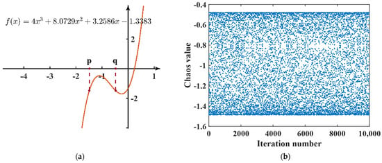
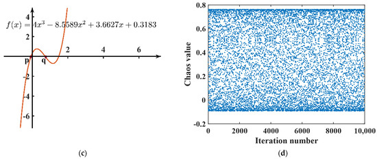
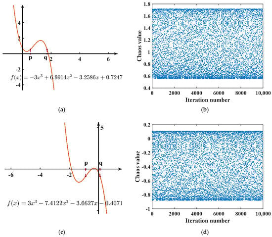
Take the parameters $a=4$ and $v=5$, respectively, and substitute them into the two cases of condition (1) of Theorem 3. The calculation can be obtained in case (i) $-2.3073\le u\le 1$; in case (ii), $-0.4334\le u\le 1$. Here, we take $u=0.4$, and the results of substituting the three parameters into condition (1) are shown in Table 1, and the function graph and the chaotic scatter plot of $x_n$ obtained from $n=10,000$ iterations are shown in Figure 1.

Table 1. Calculated results of the parameters of the three mappings under condition (1).

Parameters and Function Equations	Condition (1)
	Case (i)	Case (ii)
$\theta$	2.2616	1.7344
$b$	8.0729	−8.5589
$c$	3.2586	3.6627
$d$	−1.3383	0.3183
$p$	−1.4874	−0.0915
$q$	−0.4785	0.7624
$\phi \left(x\right)=a{x}^3+b{x}^2+cx+d$	$\phi \left(x\right)=4x^3+8.0729x^2$ $+3.2586x-1.3383$	$\phi \left(x\right)=4x^3-8.5589x^2$ $+3.6627x+0.3183$
Lyapunov exponent values	1.2117	1.3932

Figure 1. The cubic chaos mapping under condition (1): (a) Case (i) function graph; (b) scatter plot of the case (i) at $x_0=-1$; (c) case (ii) function graph; (d) scatter plot of case (ii) at $x_0=0$.

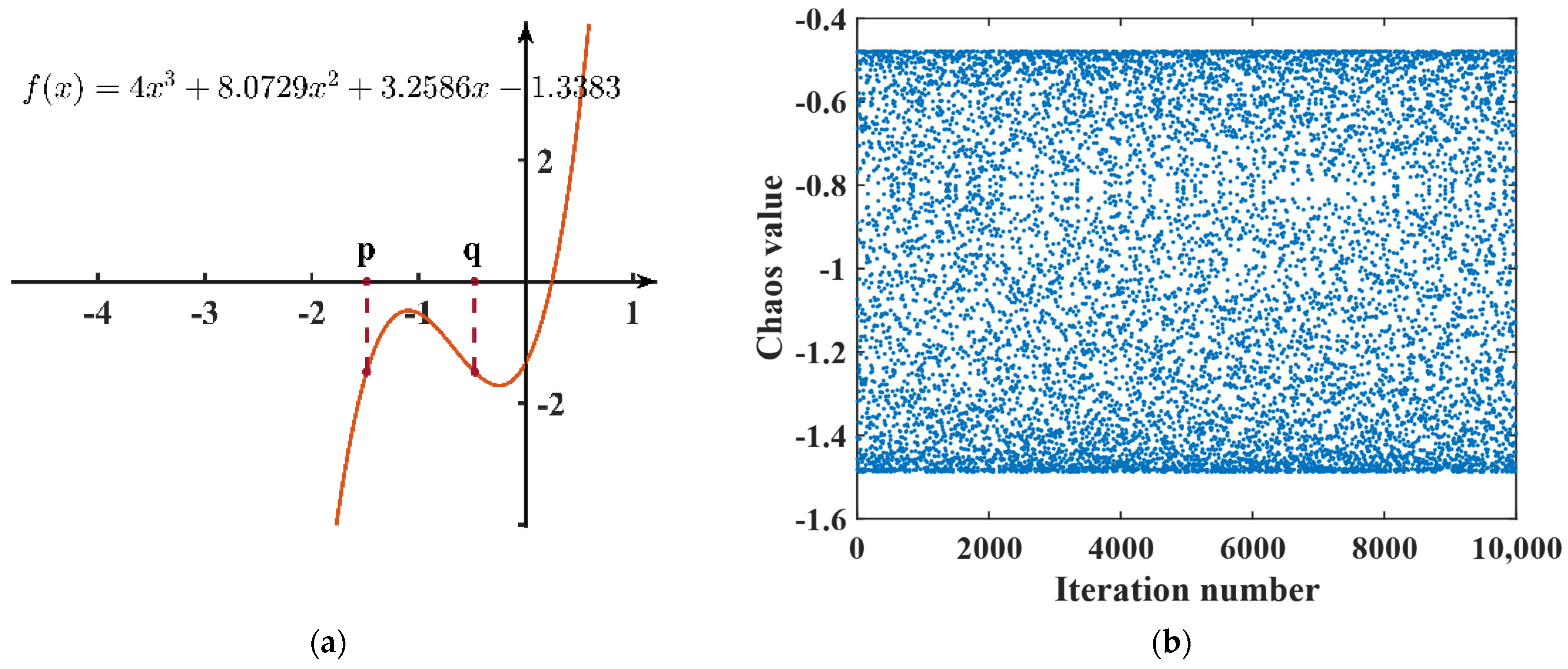
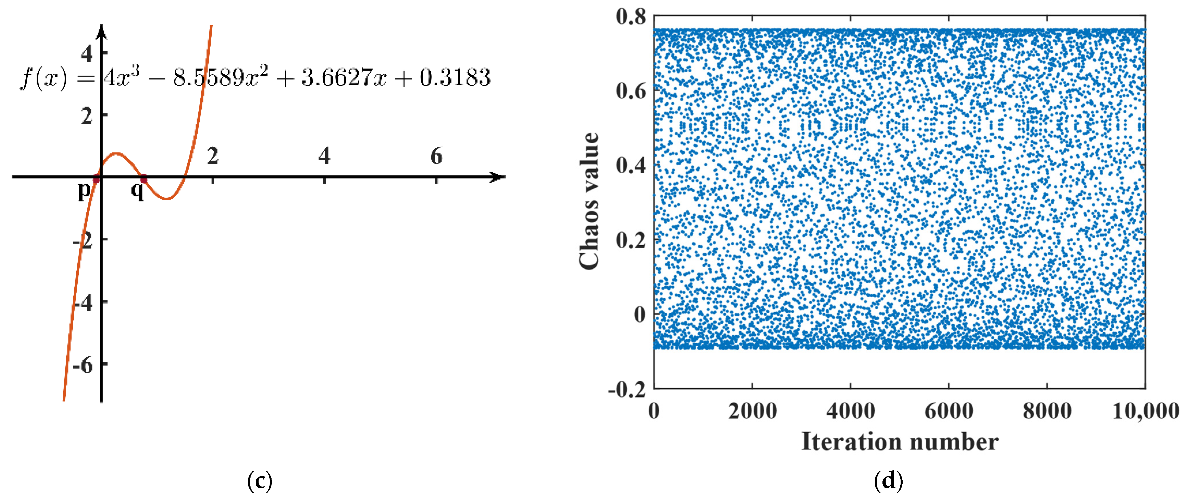
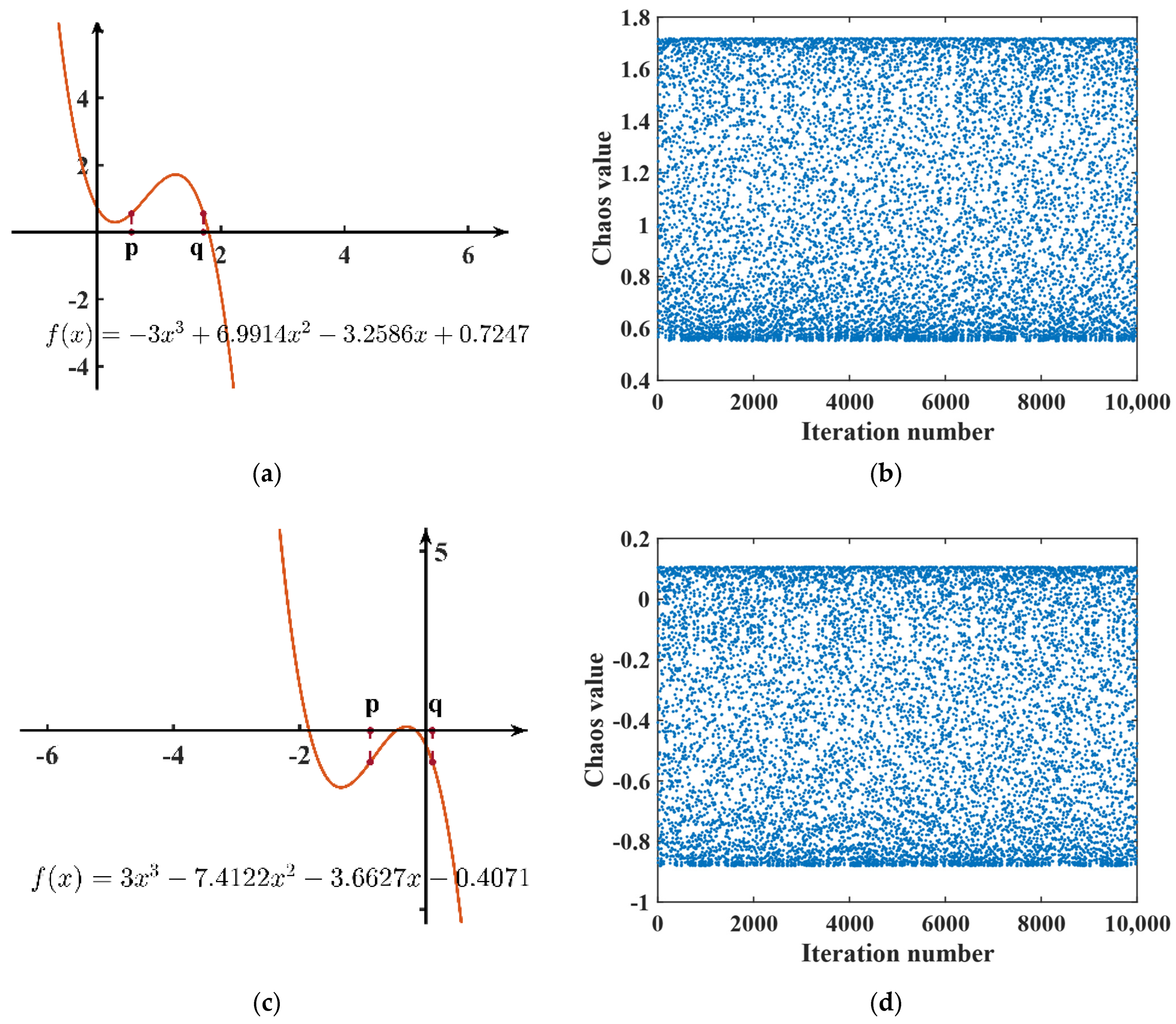
Take the parameters $a=-3$ and $v=5$, respectively, and substitute them into the two cases of condition (2) of Theorem 3. The calculation can be obtained in case (i) $-2.3073\le u\le 1$; in case (ii), $-0.4334\le u\le 1$. So here, we still take $u=0.4$, the calculation results by substituting the three parameters into condition (2) are shown in Table 2, and the function graph and the chaotic scatter plot of $x_n$ obtained by $n=10,000$ iterations are shown in Figure 2.

Table 2. Calculation results of three mapping parameters under condition (2).

Parameters and Function Equations	Condition (2)
	Case (i)	Case (ii)
$\theta$	2.2616	1.7344
$b$	6.9914	−7.4122
$c$	−3.2586	−3.6627
$d$	0.7247	−0.4071
$p$	0.5525	−0.8803
$q$	1.7175	0.1057
$\phi \left(x\right)=a{x}^3+b{x}^2+cx+d$	$\phi \left(x\right)=-3x^3+6.9914x^2$ $-3.2586x+0.7247$	$\phi \left(x\right)=-3x^3-7.4122x^2$ $-3.6627x-0.4071$
Lyapunov exponent value	1.7143	1.6480

Figure 2. The cubic chaos mapping under condition (2): (a) Case (i) function plot; (b) scatter plot of the case (i) at $x_0=1$; (c) case (ii) function plot; (d) scatter plot of the case (ii) at $x_0=0$.

From Figure 1 and Figure 2, it can be seen that $v>3$. If the parameters satisfy any of the conditions of Theorem 3, the chaotic phenomenon is generated in the interval $\left[p,q\right]$, so the chaotic system has good ergodicity, as well as unpredictability.

3. An Improved Chaotic Mapping

Here, we introduce a one-dimensional iterative chaotic folding mapping (ICMIC) [30].

$$x_{n+1}=f\left(m,x_n\right)=\sin \left({\displaystyle \frac{m}{x_n}}\right)$$

$$-1\le x_n\le 1x_0\ne 0$$

$$m\in \left(0,+\infty \right)n=0,1,2,\dots$$

(45)

where $m$ is an adjustable parameter. Since the simple chaotic mapping still has nonlinear dynamic behavior after the multiplication operation, we propose an improved chaotic mapping with the expression

$$x_n=\sin \left({\displaystyle \frac{m}{\left(af{(x_{n-1})}^3+bf{(x_{n-1})}^2+cf\left(x_{n-1}\right)+d\right)}}\right)$$

(46)

where $m\in \left(0,+\infty \right)$, the $f$ is a segmented function, and the chaotic intervals are $\left[p_1,q_1\right]$.

$$f\left(x\right)=\left\{\begin{array}{ll}p+\left|{\displaystyle \frac{x-p}{x-q}}\right|\left(q-p\right),\hfill & x<p,\hfill \\ x,\hfill & p\le x\le q,\hfill \\ p+\left|{\displaystyle \frac{x-q}{x-p}}\right|\left(q-p\right),\hfill & x>q;\hfill \end{array}\right.$$

(47)

where $a,b,c,d\in R$ satisfies Theorem 3.

The dynamics analysis of chaotic systems is of great application. In this section, scatter diagrams, histograms, bifurcation diagrams, complexity analysis, and Lyapunov exponent are chosen to measure the properties of chaotic systems.

In this section, take each parameter as $a=14$, $b=11.3923$, $c=0.9270$, $d=-0.7153$, $v=10$, and $u=0.4$. The calculation gives $p=-0.7233$ and $q=-0.0807$, taking the initial value $x=-1$ and substituting them into Equation (46) for 20,000 iterations.

3.1. Lyapunov Exponent and Bifurcation

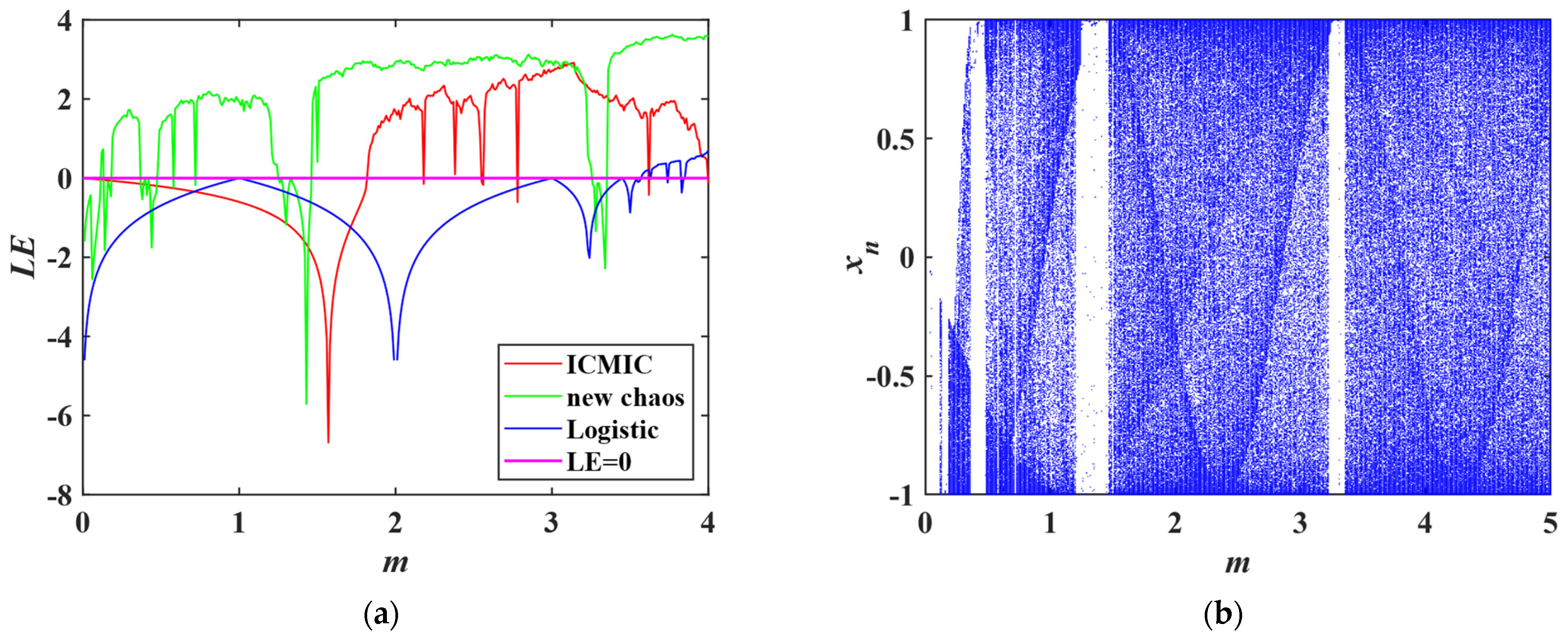
The Lyapunov exponent is an index that describes the stability of a dynamical system. The Lyapunov exponent can be used to measure the exponential growth rate between two adjacent trajectories in a dynamical system. The larger it is, the stronger and more unstable the chaotic nature of the system. Figure 3a shows the Lyapunov exponent plots of system (46), the ICMIC system, and Logistic map with respect to the state variable $m$. When the Lyapunov exponent is greater than 0, it indicates that the system is chaotic. From the graph, it can be seen that system (46) enters the chaotic state from $m=0.12$. However, the ICMIC system enters the chaotic state only after $m=1.82$. Thus, system (46) exhibits a larger chaotic range and a larger Lyapunov exponent. A bifurcation diagram is a graph used to describe the stability and chaotic nature of a dynamical system. In the bifurcation diagram, we can observe the different stability and periodicity of the system states, as well as the bifurcation phenomena that occur as the parameter values change. Figure 3b shows the bifurcation diagram with respect to the state variable $m$. From the figure, it can be seen that system (46) has a relatively uniform chaotic region and a small period window, reflecting its better chaotic characteristics. Combining Figure 3a,b, it can be concluded that, compared with ICMIC mapping, the newly constructed chaotic mapping has a wider range of parameters and stronger chaotic properties.

Figure 3. (a) Lyapunov exponent diagram. (b) Bifurcation diagram.

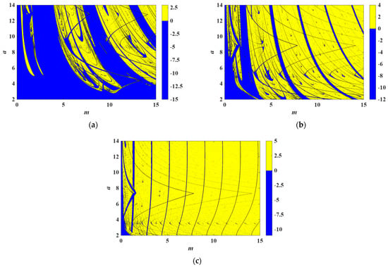
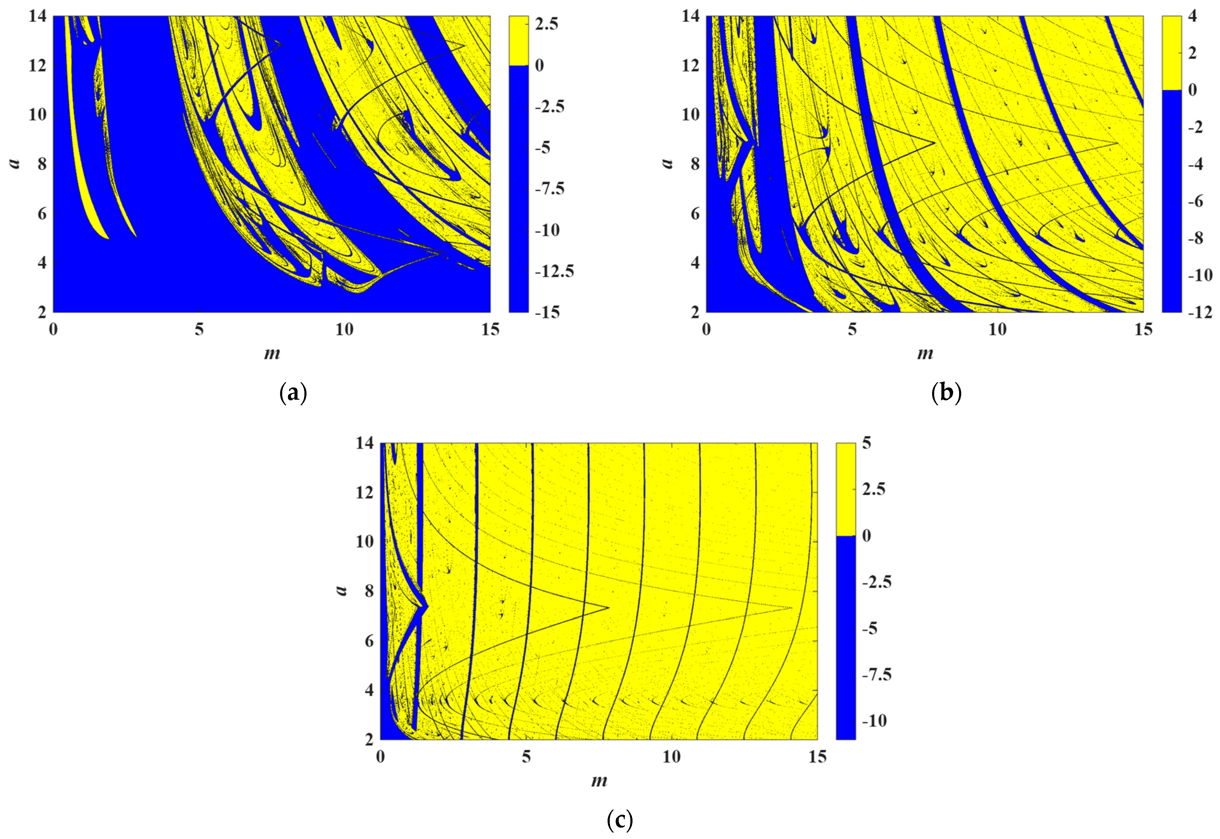
Figure 4 shows the two-parameter Lyapunov exponential diagram of system (46) with respect to the parameters $m$ and $a_1$. The system has more non-chaotic regions in Figure 4a and fewer non-chaotic regions in Figure 4b. In Figure 4c, almost all of them are chaotic regions. This indicates that the chaotic characteristics of the chaotic mapping under the control of parameters $m$ and $a$ are stronger with the increase in $v$.

Figure 4. Two-parameter Lyapunov exponent diagram about $a$ and $m$ (a) when $v=4$; (b) when $v=5$; (c) when $v=10$.

3.2. Trajectory and Scatter Plots

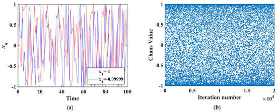
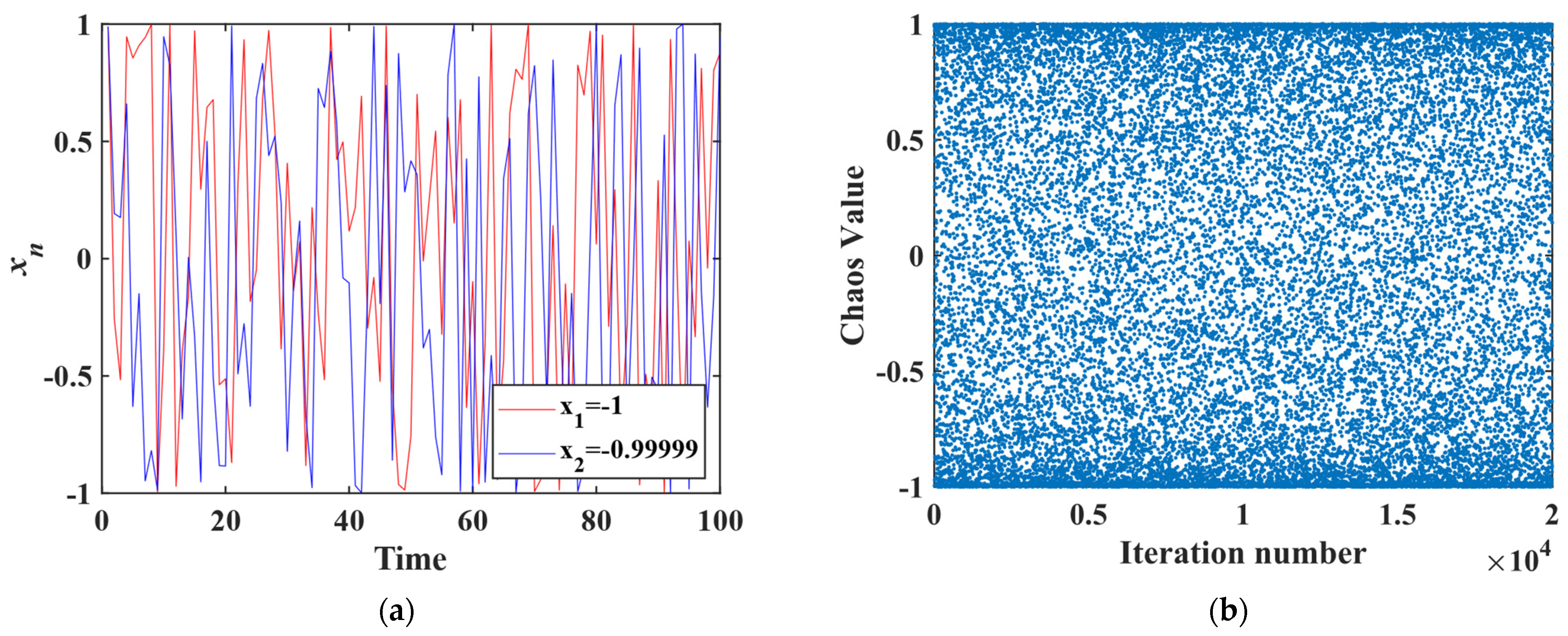
The initial value sensitivity of chaotic systems refers to the fact that small changes in the initial conditions may lead to significant differences in the evolution of the system. To analyze the initial value sensitivity of the chaotic system, we plotted the initial value sensitivity trajectory. Figure 5a shows a plot of the initial value sensitivity trajectory of system (46) for an initial value deviation of 0.00001 and $m=50$. Even if the initial value changes by only 0.00001, the trajectory of the system still varies significantly. Chaotic scatter diagrams demonstrate the nonlinear and unpredictable nature of chaotic systems by presenting their states as scatter diagrams. Figure 5b shows the scatter plot of system (46) at $m=50$, from which the ergodic and random nature of this chaotic system can be seen.

Figure 5. (a) Trajectory plot. (b) Scatter plot.

3.3. Spectral Entropy (SE) Analysis

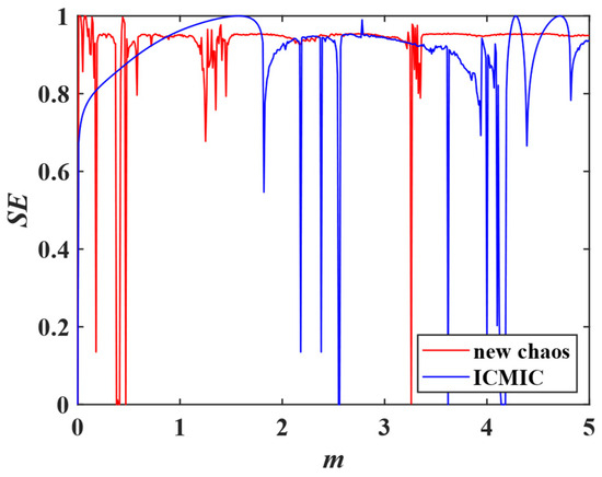
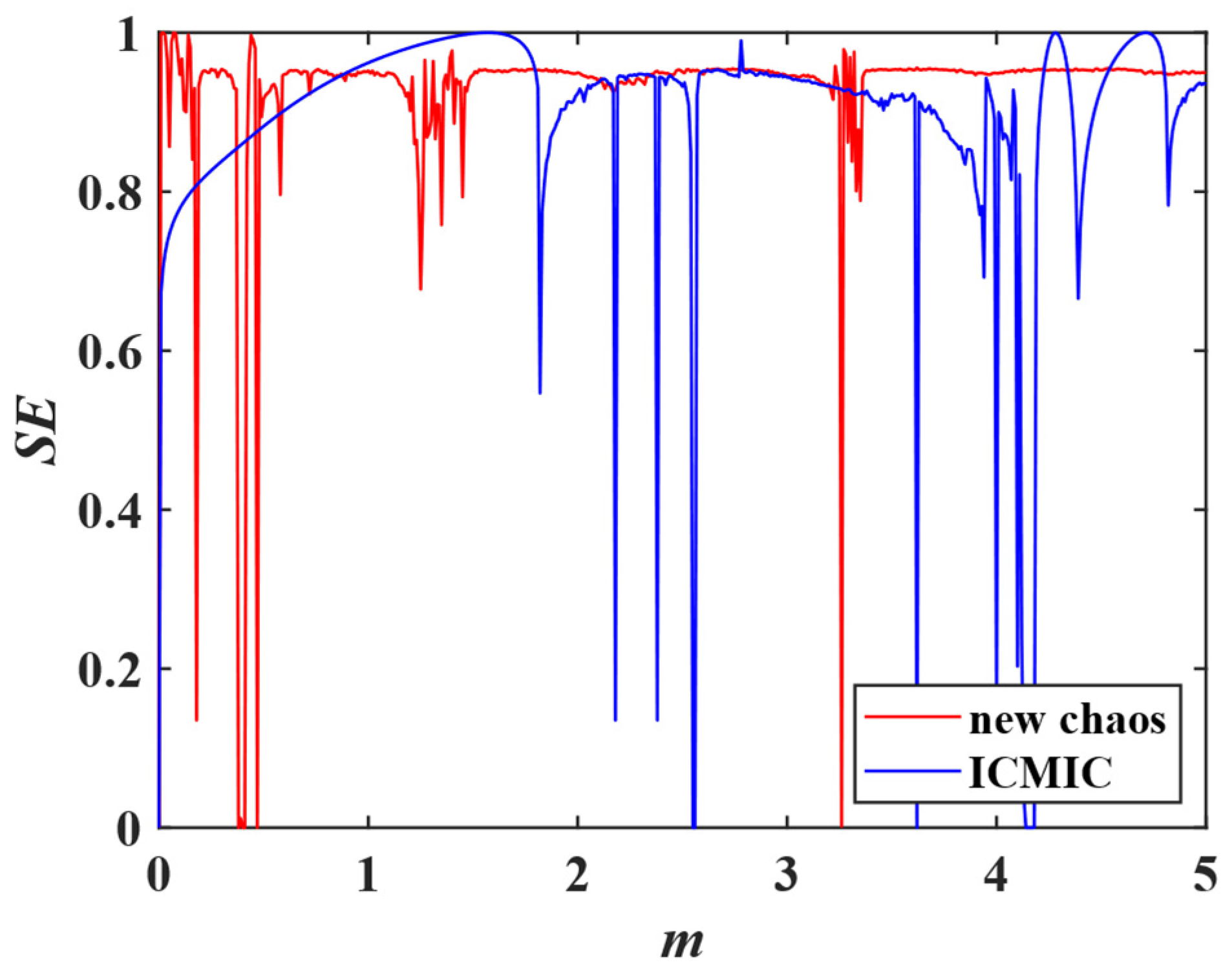
SE is an algorithm used to evaluate the complexity of chaotic systems, and its results reflect the randomness and complexity of the dynamical behavior of chaotic systems. The SE algorithm is based on the method of spectral analysis, where the power spectrum of a signal is obtained in a certain frequency band and its SE is calculated. Figure 6 shows the SE plots of system (46) and the ICMIC system with respect to the state variable $m$. As shown in the figure, the spectral entropy (SE) complexity curve of the ICMIC system exhibits significant fluctuations, with limited stable intervals. The SE of system (46) fluctuates in a relatively stable manner in the interval $\left[1.48,3.18\right]$ and $\left[3.36,5\right]$ in small increments. On the interval $\left[0,5\right]$, the SE value of system (46) is similar in size to that of the ICMIC system, but the SE value of system (46) is less volatile. Therefore, system (46) has a better stability in SE complexity. In cryptography, larger SE complexity can provide higher randomness and unpredictability and increase the resistance of cryptographic algorithms. However, in control systems or communication systems, larger SE complexity may lead to instability or uncontrollability of the system. In this case, stability and controllability are more important, so chaotic mapping with moderate SE complexity needs to be selected. It is important to note that a stable SE complexity does not mean that the system lacks complexity or randomness. Stable SE complexity simply means that the system is moderately sensitive to changes in initial conditions and parameters, and it is able to maintain a certain degree of complexity as well as the stability and controllability of the system. It can be seen that system (46) is more suitable for application in control systems or communication systems.

Figure 6. SE complexity diagram.

3.4. 0–1 Test

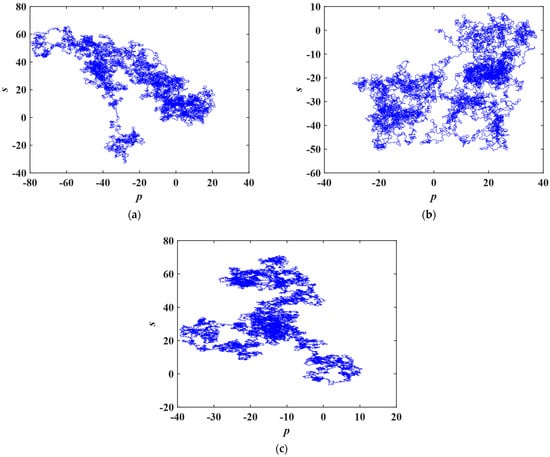
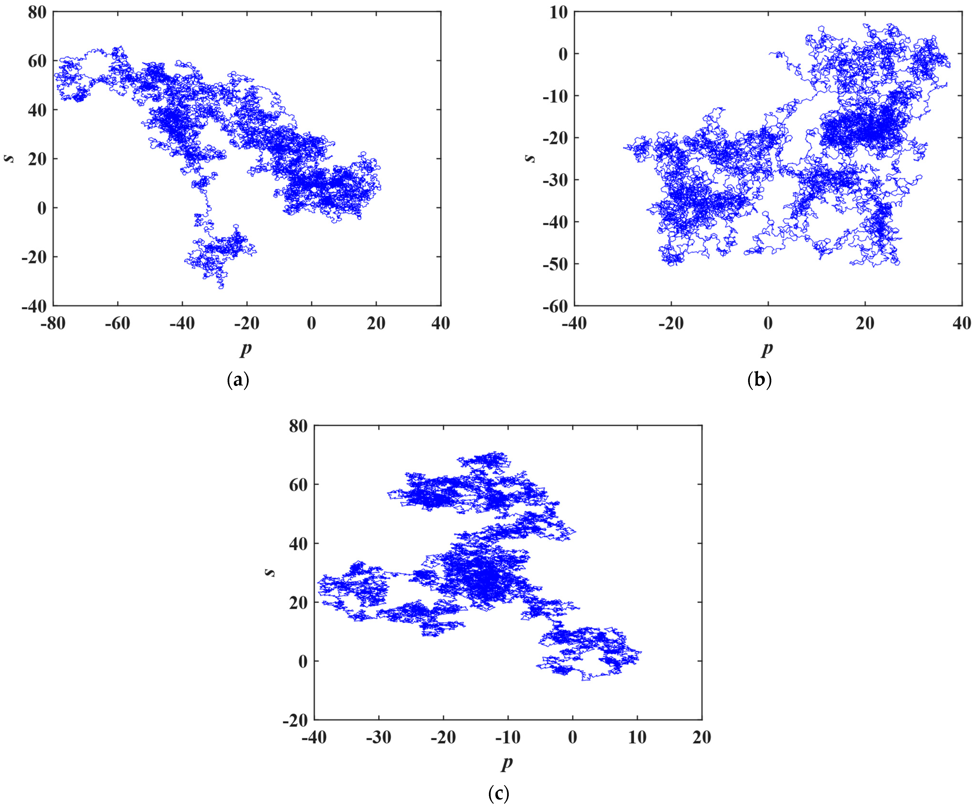
For system (46) with fixed parameters and initial values, we conduct the 0–1 test for chaos, with comparative analysis against ICMIC and the standard Logistic map. Figure 6 presents the phase diagrams for both systems.

Figure 7 reveals that the phase diagrams for system (46) exhibit Brownian-like motion with significantly greater complexity than those of ICMIC and the Logistic map. Table 3 presents the results of spectral entropy (SE) and 0–1 test for system (46), ICMIC, and the Logistic map. The data further confirm the superior chaotic performance of system (46) over ICMIC and the Logistic map.

Figure 7. The $\left(p,s\right)$ phase diagrams. (a). New Chaos. (b). ICMIC. (c). Logistic map.

Table 3. The results of SE and 0–1 test for system (46), ICMIC, and the Logistic map.

Indexes	System (46)	ICMIC	Logistic Map
SE	0.9459	0.9437	0.9351
Kc	0.8832	0.7947	0.7526
Kcreg	0.8833	0.7948	0.7525
KcCorr	0.9956	0.9606	0.9991

4. Conclusions

This paper first establishes and rigorously proves a robust chaos criterion for a class of cubic chaotic maps in the real number field. Theoretical analysis and numerical simulations confirm that the constructed maps can generate highly complex chaotic sequences with good pseudo-randomness. Secondly, by combining the structure of the infinite folding map, a novel one-dimensional discrete chaotic map is proposed. Through systematic evaluation using various dynamical analysis tools—including Lyapunov exponents, bifurcation diagrams, and spectral entropy complexity—the new map is shown to outperform traditional maps in terms of chaotic range, sensitivity to initial conditions, and sequence randomness. This study provides a clearly structured and dynamically superior mapping model for designing high-security chaotic cryptosystems, contributing positively to the application of chaos-based encryption in practical communication and information security. Future work will further explore the performance and implementation optimization of this map in scenarios such as image encryption and lightweight cryptographic protocols.

References

- May, R.M. Simple mathematical models with very complicated dynamics. Nature 1976, 261, 459–467. [Google Scholar] [CrossRef] [Scilit]
- Liao, G.; Wang, L. Almost periodicity, chain recurrence and chaos. Isr. J. Math. 1996, 93, 145–156. [Google Scholar] [CrossRef] [Scilit]
- Hoppe, V. Specification of geometrical parameters for elements with cubic mapping functions. Int. J. Numer. Methods Eng. 1973, 7, 94–98. [Google Scholar] [CrossRef] [Scilit]
- Zhao, H.; Xie, S.; Zhang, J.; Wu, T. A Dynamic Block Image Encryption Using Variable-Length Secret Key and Modified Henon. Map. Opt. 2021, 230, 166307. [Google Scholar] [CrossRef] [Scilit]
- Feng, W.; Tang, Z.; Zhao, X.; Qin, Z.; Chen, Y.; Cai, B.; Zhu, Z.; Qian, K.; Wen, H. Two-Dimensional Coupling-Enhanced Cubic Hyperchaotic Map with Exponential Parameters: Construction, Analysis, and Application in Hierarchical Significance-Aware Multi-Image Encryption. Axioms 2025, 14, 901. [Google Scholar] [CrossRef] [Scilit]
- Sun, J. 2D-SCMCI Hyperchaotic Map for Image Encryption Algorithm. IEEE Access 2021, 9, 59313–59327. [Google Scholar] [CrossRef] [Scilit]
- Elrefai, H.M.; Sayed, W.S.; Said, L.A. Hardware-based audio encryption system using two-dimensional chaotic maps. Electronics 2024, 13, 4254. [Google Scholar] [CrossRef] [Scilit]
- Alexan, W.; El Shabasy, N.H.; Ehab, N.; Mohamed, A. A chaos-based augmented image encryption scheme for satellite images using Fredkin logic. Sci. Rep. 2025, 15, 22008. [Google Scholar] [CrossRef] [Scilit] [PubMed]
- Mansoor, S.; Sarosh, P.; Ali, R.; Khan, M.A. Adaptive color image encryption using multiple distinct chaotic maps and DNA computing. Mathematics 2022, 10, 2004. [Google Scholar] [CrossRef] [Scilit]
- Kwok, H.S.; Tang, W.K. A fast image encryption system based on chaotic maps with an improved diffusion mechanism. Chaos Solitons Fractals 2007, 32, 1518–1529. [Google Scholar] [CrossRef] [Scilit]
- Li, C.; Xie, T.; Liu, Q. Cryptanalyzing image encryption using chaotic logistic map. arXiv 2013, arXiv:1301.4089. [Google Scholar] [CrossRef] [Scilit]
- Feng, W.; Tang, Z.; Zhao, X.; Qin, Z.; Chen, Y.; Cai, B.; Zhu, Z.; Wen, H.; Ye, C. State-Dependent Variable Fractional-Order Hyperchaotic Dynamics in a Coupled Quadratic Map: A Novel System for High-Performance Image Protection. Fractal Fract. 2025, 9, 792. [Google Scholar] [CrossRef] [Scilit]
- Machicao, J.; Alves, M.; Brunnet, L.G. Exploiting ergodicity of logistic map using deep-zoom to improve chaos-based cryptosystems. arXiv 2018, arXiv:1808.02949. [Google Scholar] [CrossRef] [Scilit]
- Kocarev, L.; Jakimoski, G. Logistic map as a block encryption algorithm. Phys. Lett. A 2001, 289, 199–206. [Google Scholar] [CrossRef] [Scilit]
- Song, X.; Xu, D.; Li, G.; Xu, W. Multi-image reorganization encryption based on SLF cascade chaos and bit scrambling. J. Web Eng. 2021, 20, 1177–1192. [Google Scholar] [CrossRef] [Scilit]
- Alawida, M. Enhancing logistic chaotic map for improved cryptographic security in random number generation. J. Inf. Secur. Appl. 2024, 80, 103685. [Google Scholar] [CrossRef] [Scilit]
- Hosny, K.M.; Elnabawy, Y.M.; Salama, R.A.; Elshewey, A.M. Multiple image encryption algorithm using channel randomization and multiple chaotic maps. Sci. Rep. 2024, 14, 30597. [Google Scholar] [CrossRef] [Scilit] [PubMed]
- Fedoseev, P.; Pesterev, D.; Rozhkov, V.; Rybin, V.; Butusov, D. Chaotic encryption algorithm based on Gingerbreadman map with adaptive symmetry. Chaos Theory Appl. 2025, 7, 31–41. [Google Scholar] [CrossRef] [Scilit]
- Kopp, M.; Samuilik, I. Dynamical analysis and adaptive synchronization of a new 6D hyperchaotic system with the cosine function. Math. Model. Anal. 2025, 30, 626–644. [Google Scholar] [CrossRef] [Scilit]
- Huang, G.C. Efficient parameter search for chaotic dynamical systems using reinforcement learning. Symmetry 2025, 17, 1832. [Google Scholar] [CrossRef] [Scilit]
- Xu, J.; Li, C.; Cen, X.; Zhang, X.; Chai, L. Chaos regulation via complex nonlinear feedback and its implementation based on FPAA. Symmetry 2025, 17, 212. [Google Scholar] [CrossRef] [Scilit]
- Yu, F.; Kong, X.; Yao, W.; Zhang, J.; Cai, S.; Lin, H.; Jin, J. Dynamics analysis, synchronization and FPGA implementation of multiscroll Hopfield neural networks with non-polynomial memristor. Chaos Solitons Fractals 2024, 179, 114440. [Google Scholar] [CrossRef] [Scilit]
- Weissenbacher, M.; Borovykh, A.; Rigas, G. Reinforcement learning of chaotic systems control in partially observable environments. Flow Turbul. Combust. 2025, 115, 1357–1378. [Google Scholar] [CrossRef] [Scilit]
- An, X.; Li, D.; Li, J. An improved chaos control with adaptive active set approach combined in reliability-based design optimization. Sci. Rep. 2025, 15, 42790. [Google Scholar] [CrossRef] [Scilit]
- Rojas-Galván, R.; Mercado-Gutiérrez, E.; Tlelo-Cuautle, E. Optimizing chaotic systems by orbit counting and Fourier spectrum: FPGA implementation and image encryption application. Math. Model. Anal. 2025, 30, 322–341. [Google Scholar] [CrossRef] [Scilit]
- Al-Barakati, A.A.; Mesdoui, F.; Bekiros, S.; Kaçar, S.; Jahanshahi, H. A variable-order fractional memristor neural network: Secure image encryption and synchronization via a smooth and robust control approach. Chaos Solitons Fractals 2024, 186, 115135. [Google Scholar] [CrossRef] [Scilit]
- Xu, W.; Chen, X.; Zhou, Z.; Li, G.; Song, X. General construction method and proof for a class of quadratic chaotic mappings. Mathematics 2025, 13, 2409. [Google Scholar] [CrossRef] [Scilit]
- Qi, C.; Bi, Y.; Han, H.; Li, Y. A hybrid particle swarm optimization algorithm. In Proceedings of the 2017 3rd IEEE International Conference on Computer and Communications (ICCC); IEEE: Piscataway, NJ, USA, 2017; pp. 2187–2190. [Google Scholar] [CrossRef] [Scilit]
- Andrecut, M.; Ali, M.K. Robust chaos in smooth unimodal maps. Phys. Rev. E 2001, 64, 025203. [Google Scholar] [CrossRef] [Scilit] [PubMed]
- He, D.; He, C.; Jiang, L.G.; Zhu, H.W.; Hu, G.R. Chaotic characteristics of a one-dimensional iterative map with infinite collapses. IEEE Trans. Circuits Syst. I Fundam. Theory Appl. 2001, 48, 900–906. [Google Scholar] [CrossRef] [Scilit]
Disclaimer/Publisher’s Note: The statements, opinions and data contained in all publications are solely those of the individual author(s) and contributor(s) and not of MDPI and/or the editor(s). MDPI and/or the editor(s) disclaim responsibility for any injury to people or property resulting from any ideas, methods, instructions or products referred to in the content. |
© 2026 by the authors. Licensee MDPI, Basel, Switzerland. This article is an open access article distributed under the terms and conditions of the Creative Commons Attribution (CC BY) license.