On Equiresistant Graphs

Abstract

We say a finite simple connected undirected graph is equiresistant if all its edges have the same effective resistance when the graph is considered as an electric circuit where the edges are unit resistors. Using simple properties of electric circuits, we identify some new families of graphs that are equiresistant and then apply this knowledge to find upper bounds for some molecular indices that improve; in the case of equiresistant graphs, similar upper bounds are found in the literature.

1. Introduction

In this article, a graph $G=(V,E)$ is meant to be a finite simple connected undirected graph with vertex set $V=\{1,2,\dots ,n\}$, edge set E, and vertex degrees $d_1,d_2,\dots ,d_n$. Reference [1] contains everything that is needed from graph theory in what follows below.

In mathematical chemistry, molecules are modeled using these graphs, where the atoms are represented by the vertices and the atomic bonds are represented by the edges. Many topological indices, or descriptors, i.e., real-valued functions on the domain of all graphs, have been introduced with the goal of capturing physico-chemical properties of the molecules and classifying them according to the values of their indices. One such index is the Kirchhoff index defined in [2] as follows:

$$K\left(G\right)=\sum _{i<j}{R}_{ij},$$

(1)

where $R_{ij}$ is the effective resistance between vertices i and j when the graph is thought of as an electrical network and all the edges have a resistance of 1 Ohm. In order to study this index, it is essential to study properties of effective resistances, and we point to references [3,4,5,6] and their bibliography that do precisely that. The Kirchhoff index may be thought of as an extension of the classical Wiener index (see [7]), given by the sum of the distances between all vertices. More formally, the distance $d(i,j)$ between vertices i and j is the length of a shortest walk between i and j, and the Wiener index is defined as follows:

$$W\left(G\right)=\sum _{i<j}d(i,j).$$

It is not difficult to show that $K\left(T\right)=W\left(T\right)$ for any tree T.

On the graph G, one can define the simple random walk as the Markov chain $\{X_n,n\ge 0\}$ with state space V and uniform transition probabilities from a given vertex i to one of its $d_i$ neighboring vertices. The hitting time $T_j$ of the vertex j is defined as the infimum of the number of transitions needed by the random walk to get to the vertex j:

$$T_j=inf\{n\ge 0:X_n=j\},$$

and its expectation when the process starts at state i is denoted by $E_i{T}_j$. Reference [8] contains a good introduction to hitting times of Markov chains.

There is a close relationship between hitting times and the Kirchhoff index that we studied in [9], summarized in the following equation:

$$K\left(G\right)={\displaystyle \frac{1}{2\left|E\right|}}\sum _{i<j}(E_i{T}_j+E_j{T}_i),$$

(2)

thus providing probabilistic intuitions and tools to study this index. Reference [10] is a good introduction to the connection between electric networks and random walks on graphs.

We defined in [11] the hitting time index of a graph G, $HT\left(G\right)$, as follows:

$$HT\left(G\right)=\sum _{i<j}D(i,j),$$

where $D(i,j)=max\{E_i{T}_j,E_j{T}_i\}$. Among other things, we showed that the $HT$ index is related to the other indices in this introduction through the following inequalities, valid for any graph G:

$$K\left(G\right)\le W\left(G\right)\le HT\left(G\right)\le 2\left|E\right|K\left(G\right).$$

(3)

We say that a graph is equiresistant if all its edges have the same effective resistance, i.e., if the effective resistance between the endpoints of any edge is the same. In what follows, we will identify a large family of such graphs and will see how the leftmost inequality in (3) is improved in the context of these equiresistant graphs and how we get a set of inequalities linking $W\left(G\right)$ and $HT\left(G\right)$ similar to the two rightmost inequalities in (3), again in the context of equiresistant graphs. The main tools of electric circuits that we will be using are the facts that the effective resistance of two resistors connected in series is the sum of the individual resistances, whereas the effective resistance between the endpoints of two resistors set in parallel is the inverse of the sum of the inverses of the individual resistances. We will also use the fact that vertices with the same voltage can be shorted, that is, fused into a single vertex, while deleting all edges between the vertices being shorted.

2. The Results

The basic hypothesis in our graphs is that all the edges are resistors with unit resistance. In order to find the effective resistance of an edge $(a,b)\in E$, denoted by $R_{ab}$, we must find the inverse of the current $i_a$ established between the endpoints a and b of said edge when a battery is installed so that the voltage at one end is $v_a=1$ and the voltage at the other end is $v_b=0$. If the edge $(a,b)$ belongs to a tree, since the tree has no cycles, the total current $i_a$ entering a can only go directly from a to b through the edge $(a,b)$, and using Ohm’s law, we get $i_a={\displaystyle \frac{v_a-v_b}{1}}=1$. Therefore, the effective resistance of the edge $(a,b)$ is $R_{ab}={\displaystyle \frac{1}{i_a}}=1$, and this being valid for any edge in any tree means that all trees are equiresistant, and the common value of all effective resistances is 1.

Foster’s first formula (see [12]), says that for any graph $G=(V,E)$, the sum of the effective resistances over all edges is a constant, independent of the graph chosen. Indeed:

$$\sum _{(a,b)\in E}{R}_{ab}=n-1.$$

If G is equiresistant then Foster’s formula implies the following:

$$R_{ab}={\displaystyle \frac{n-1}{\left|E\right|}},$$

(4)

for all $(a,b)\in E$. We will call this number Foster’s resistance, and since it does not depend on the edge chosen, we will denote it by $R_F\left(G\right)$. If G is a tree T, (4) says $R_F\left(T\right)=1$, which coincides with the result obtained with electric principles above. For any other equiresistant graphs, $R_F\left(G\right)<1$.

In addition to the trees, one may ask which other graphs are equiresistant. The following result is known rather well (see [3,12,13]). Informally, it says that if the electric circuit looks the same when seen from any two edges, then the effective resistances of those edges are the same.

Proposition 1.

If G is an edge transitive graph then it is equiresistant.

For the next results, given the graphs $G_1=(V_1,E_1)$ and $G_2=(V_2,E_2)$, we define the new graph $G_1$ conjoined to $G_2$ through the vertices $v_1,v_2,\dots ,v_k$ as the graph $G=(V,E)$, where $V=V_1\cup V_2$, $E=E_1\cup E_2$ and $V_1\cap V_2=\{v_1,v_2,\dots ,v_k\}$.

Proposition 2.

If G is the result of conjoining at a single vertex two equiresistant graphs $G_1=(V_1,E_1)$ and $G_2=(V_2,E_2)$, with $R_F\left(G_1\right)=R_F\left(G_2\right)$, then G is equiresistant, and $R_F\left(G\right)=R_F\left(G_1\right)=R_F\left(G_2\right)$.

Proof. 

Let us consider $(i,j)\in E$ and suppose first that $(i,j)\in E_1$. When we compute $R_{ij}$, we set up a battery between vertices i and j so that the voltage at i is 1 and the voltage at j is 0. Then we find the total current $I_i$ flowing out of i and $R_{ij}=I_i^{-1}$. But by the form in which G is built, we can short all the vertices of $G_2$ into the single vertex where $G_2$ is conjoined to $G_1$, because all the vertices in $G_2$ have the same voltage as that of the vertex where the graphs are conjoined, and therefore the computation of $R_{ij}$ over the circuit defined by G is the same as the computation over the circuit defined by $G_1$, and thus $R_{ij}={\displaystyle \frac{n_1-1}{|E_1|}}$. Now, if $(s,t)\in E$ and in fact $(s,t)\in E_2$, by a similar argument $R_{st}={\displaystyle \frac{n_2-1}{|E_2|}}$.

But the hypothesis is the following:

$${\displaystyle \frac{n_1-1}{|E_1|}}={\displaystyle \frac{n_2-1}{|E_2|}},$$

(5)

so regardless of where the edge is, either in $E_1$ or in $E_2$, we get the same value for the effective resistance of the edge, and this common value is therefore equal to $R_F\left(G\right)$.

Also, we can double-check that, since $G=(V,E)$ satisfies $\left|V\right|=n_1+n_2-1$ and $\left|E\right|=|E_1|+|E_2|$, we have the following:

$$R_F\left(G\right)={\displaystyle \frac{\left|V\right|-1}{\left|E\right|}}={\displaystyle \frac{n_1+n_2-2}{|E_1|+|E_2|}}={\displaystyle \frac{n_1-1+n_2-1}{|E_1|+|E_2|}}.$$

Solving for $n_1-1$ in (5), we get the following:

$$R_F\left(G\right)={\displaystyle \frac{1}{|E_1|+|E_2|}}\left({\displaystyle \frac{(n_2-1)\left|E_1\right|}{|E_2|}}+n_2-1\right)={\displaystyle \frac{n_2-1}{|E_2|}},$$

as expected. □

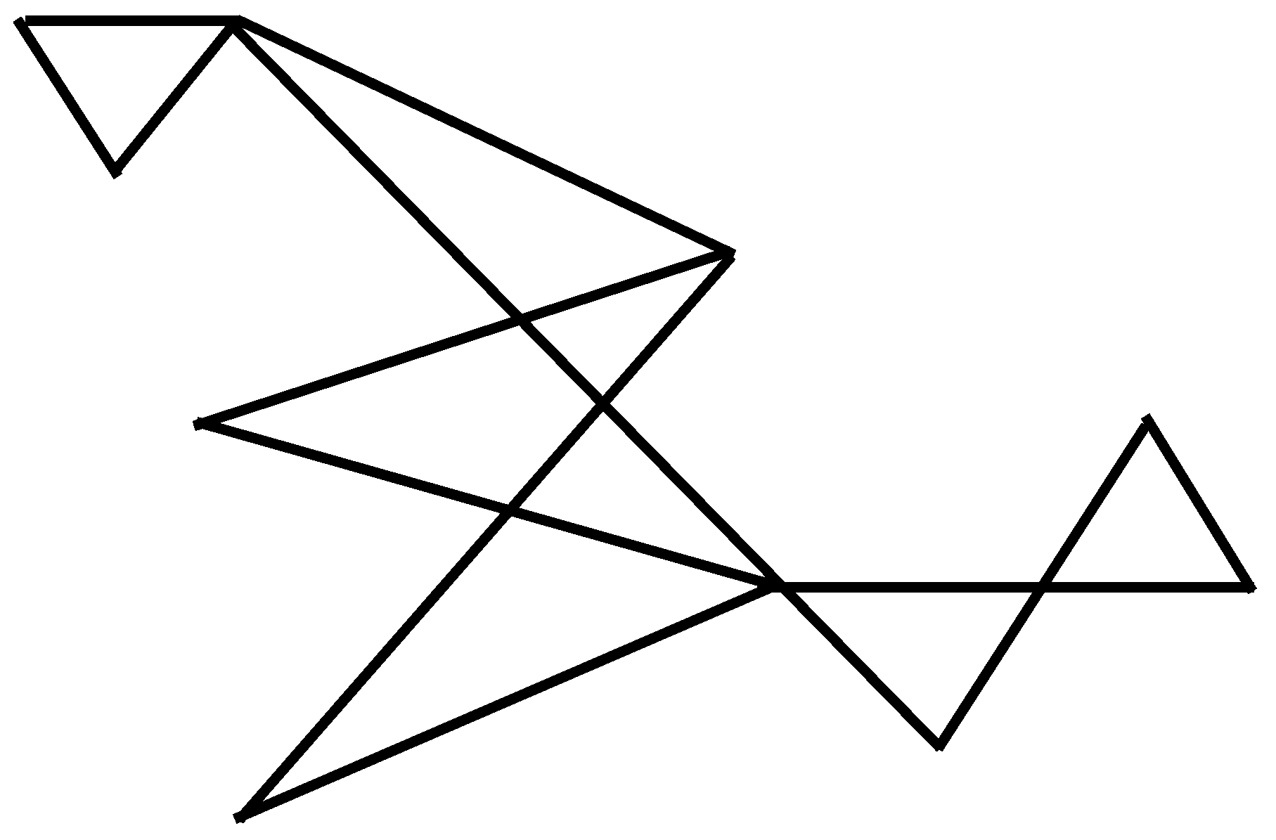
It is clear that we can iterate the procedure given in the previous proposition. For example, in Figure 1, we conjoin one complete graph $K_3$ to a complete bipartite graph $K_{2,3}$ at a vertex of degree 2, then another $K_3$ at a vertex of degree 3, and then a final $K_3$ is conjoined to the previous $K_3$ at either of its vertices of degree 2. All of these graphs have Foster’s resistance equal to ${\displaystyle \frac{2}{3}}$, so that the resulting graph also has Foster’s resistance equal to ${\displaystyle \frac{2}{3}}$. An equiresistant graph does not need to have any kind of symmetry, as this example shows: it is not edge transitive, not vertex transitive, not even regular.

So far, our catalog of equiresistant graphs consists of trees, edge-transitive graphs, and the result of conjoining several of these. One could conjecture that there are no more equiresistant graphs. To support that conjecture, we prove the following three results.

Proposition 3.

If G is a graph with $\left|V\right|=n$ and $\left|E\right|\ge n$, then it cannot have a pendant vertex or a cut edge.

Proof. 

Suppose the graph has either a cut edge or an edge one of whose vertices is a pendant vertex. Either of these edges has effective resistance equal to 1. But this value must be the value of the Foster’s resistance, which is also equal to the following:

$${\displaystyle \frac{n-1}{\left|E\right|}}<1,$$

and so we get a contradiction. □

This proposition implies the following:

Corollary 1.

The only unicyclic equiresistant graph with n vertices, for $n\ge 3$, is the n-cycle $C_n$.

Proof. 

The only n-vertex unicyclic graph without pendant vertices or cut edges is $C_n$. □

In a similar way we can prove the following:

Proposition 4.

The only n-vertex bicyclic equiresistant graph is the result of conjoining, at a single vertex, two identical cycles $C_{\lceil {\displaystyle \frac{n}{2}}\rceil }$, for $n=5,7,9,\dots$.

Proof. 

Bicyclic graphs come in essentially two basic types: ∞-type, which is obtained from connecting one vertex of one cycle to one vertex of a different disjoint cycle with a path, and $\mathsf{\Theta }$-type, where three internally disconnected paths are connected at their endpoints in such a way that at most only one path can have length 1. In addition to these two basic types of bicyclic graphs, one can attach trees to some of their vertices in order to obtain all possible bicyclic graphs.

Since an equiresistant graph cannot have pendant vertices or cut edges, the only bicyclic graphs left from the listing in the previous paragraph are the result of conjoining two cycles (of possibly different sizes) through some vertices $\{v_1,v_2,\dots v_k\}$. Let us assume first that the conjoining is done through only two vertices, $v_1,v_2$. It is obvious that unless the two cycles are of the same size, their edges other than $(v_1,v_2)$ will not have all the same effective resistance. So we can assume that we have two equal $C_n$ cycles conjoined at the vertices $v_1$ and $v_2$. Now we compute the effective resistance of the edge $(v_1,v_2)$. If we put a battery between $v_1$ and $v_2$ so that the voltage at $v_1$ is equal to 1 and the voltage at $v_2$ is equal to 0, by the symmetry of the setup, we can short pairs of vertices on both $C_n$’s, which are symmetric with respect to the edge $(v_1,v_2)$. Then, using simple transformations of resistors in series and in parallel, it is easy to see that the effective resistance we are looking for is as follows:

$$R_{v_1{v}_2}={\displaystyle \frac{n-1}{n+1}}.$$

But this is not the value of Foster’s resistance for this graph with $2n-2$ vertices and $2n-1$ edges, which should be ${\displaystyle \frac{2n-3}{2n-1}.}$ Therefore, this graph is not equiresistant. The case where the conjoining is done through more than two vertices is treated in a similar way. For example, if the two $C_n$ cycles are conjoined at the vertices $v_1,v_2$ and $v_3$, as before, we put a battery between $v_1$ and $v_2$ so that the voltage at $v_1$ is equal to 1 and the voltage at $v_2$ is equal to 0, and by the symmetry of the setup, we can short pairs of vertices on both $C_n$’s, which are symmetric with respect to the path with edges $(v_1,v_2)$ and $(v_2,v_3)$. Then, using simple transformations of resistors in series and in parallel, it is easy to see that the effective resistance we are looking for is as follows:

$$R_{v_1{v}_2}={\displaystyle \frac{n}{n+2}},$$

which is not the value of Foster’s resistance for this graph with $2n-3$ vertices and $2n-2$ edges, which should be ${\displaystyle \frac{2n-4}{2n-2}=\frac{n-2}{n-1}.}$ Therefore, this graph is not equiresistant. □

In spite of the results above for unicyclic and bicyclic graphs, the conjecture that the only equiresistant graphs are trees and edge-transitive graphs and the result of conjoining several of these at a single point is not true. The Cayley graph of the group ${\mathbb{Z}}_4\times {\mathbb{Z}}_4$ with respect to the connecting set $S=\left\{\right(i,0),(0,i),(i,i):1\le i\le 3\}$ is a distance regular graph; in fact, a strongly regular graph with parameters $(16,9,4,6)$, which is not edge transitive (see Theorem 3.1 in [14]), and it is not the conjoining of two or more graphs because it does not contain cut points, but it is equiresistant, with all edges having resistance ${\displaystyle \frac{5}{24}}$. (For completeness, the effective resistance between any pair of non-adjacent vertices is ${\displaystyle \frac{11}{48}}$).

Thus, the problem of characterizing all equiresistant graphs is far from solved, and it remains an interesting, open problem.

We should point out that there is a recent new concept, that of resistance regular graphs (see [15]), which is somewhat related to our equiresistant graphs. A graph is resistance regular when the sums of all effective resistances from one vertex to all other vertices in the graph, that is, when the following:

$$\sum _{b\in V}{R}_{ab},$$

(6)

is the same regardless of the choice of a.

These two notions are, however, different: the 3-path is an equiresistant graph, but it is not resistance regular, because the sums in (6) can be 2 or 3 depending on whether a is the midpoint or one of the endpoints. A more involved example is the 3-dimensional cube together with all the midpoints of its edges: this is a 20-vertex graph with 24 edges, which is edge transitive, and therefore equiresistant, but not resistance regular, as the sums in (6) are either 26.6667 or 29.8333, depending on whether the vertex a is chosen to have degree 3 or 2, respectively.

Conversely, the example shown in Figure 2 in [15] shows a resistance regular graph, which is not equiresistant.

Now we will apply the results found above in the next two propositions, in order to find two new upper bounds for molecular descriptors that improve those given in the introduction, when applied to equiresistant graphs. Examples of real molecules that are modeled as equiresistant graphs are the tetrahedral methane and many polyhedral boranes (see [16]).

Proposition 5.

For every equiresistant G with Foster’s resistance $R_F\left(G\right)$ we have the following:

$$K\left(G\right)\le R_F\left(G\right)W\left(G\right).$$

(7)

Proof. 

Let $i=i_1,i_2,\dots ,i_k=j$ be a shortest path between vertices i and j. By the triangular inequality for resistances (see [2]), we have the following:

$$R_{ij}\le R_{i_1{i}_2}+R_{i_2{i}_3}+\dots +R_{i_{k-1}{i}_k}=R_F\left(G\right)d(i,j).$$

(8)

Adding over all $(i,j)\in E$, we get the following:

$$K\left(G\right)\le R_F\left(G\right)W\left(G\right).$$

(9)

 □

The inequality in (7) becomes the leftmost inequality in (3) when G is a tree. In any other case, since $R_F\left(G\right)<1$, (7) is a real improvement over (3).

We conclude with another pair of inequalities linking the indices $W\left(G\right)$ and $HT\left(G\right)$. A graph is walk-regular if the number of k-long walks, $k\ge 2$, starting and ending at a vertex v is the same for all $v\in V$. This family contains, among others, all regular edge-transitive graphs. For walk-regular graphs, the following was shown in [11]:

$$HT\left(G\right)=\left|E\right|K\left(G\right).$$

This fact, and the fact that regular edge-transitive graphs are walk-regular and equiresistant, together with Equations (3) and (9), give us a proof of the following:

Proposition 6.

For any regular edge-transitive graph G we have the following:

$$W\left(G\right)\le HT\left(G\right)\le \left|E\right|R_F\left(G\right)W\left(G\right).$$

Since $R_F\left(G\right)<1$ for all graphs in this proposition, it improves what we could obtain in [11] in terms of “sandwiching” the index $HT$ in terms of the index W, which would be $W\left(G\right)\le HT\left(G\right)\le \left|E\right|W\left(G\right)$.

3. Final Remarks

In this article we introduced the notion of equiresistant graphs, exhibited some new families of equiresistant graphs, and showed how this new definition differs from the concept of resistant regular graphs. Then we showed how some inequalities for molecular descriptors are improved in the context of equiresistant graphs by the factor of Foster’s resistance. The counterexample provided to the initial conjecture that all equiresistant graphs were either trees or edge-transitive graphs or their conjoining shows us a way for future work: the complete identification of equiresistant graphs, which may include a subset of the family of distant-regular graphs and their conjoining.

References

- Buckley, F.; Harary, F. Distance in Graphs; Addison-Wesley Publishing Company: Redwood City, CA, USA, 1990. [Google Scholar]
- Klein, D.J.; Randić, M. Resistance distance. J. Math Chem. 1993, 12, 81–95. [Google Scholar] [CrossRef]
- Klein, D.J. Resistance-distance sum rules. Croat. Chem. Acta 2002, 75, 633–649. [Google Scholar]
- Palacios, J.L. Foster’s formulas via probability and the Kirchhoff index. Methodol. Comput. Appl. Probab. 2004, 4, 381–387. [Google Scholar] [CrossRef]
- Chen, H. Random walks and the effective resistance sum rules. Discret. Appl. Math. 2010, 158, 1691–1700. [Google Scholar] [CrossRef]
- Ge, J. Effective resistances and spanning trees in the complete bipartite graph plus a matching. Discret. Appl. Math. 2021, 305, 145–153. [Google Scholar] [CrossRef]
- Wiener, H. Structural determination of paraffin boiling points. J. Am. Chem. Soc. 1947, 69, 17–20. [Google Scholar] [CrossRef] [PubMed]
- Grinstead, M.; Snell, J.L. Introduction to Probability, 2nd ed.; American Mathematical Society: Providence, RI, USA, 1997. [Google Scholar]
- Palacios, J.L. Resistance distance in graphs and random walks. Int. J. Quantum Chem. 2001, 81, 29–33. [Google Scholar] [CrossRef]
- Doyle, P.G.; Snell, J.L. Random Walks and Electrical Networks; The Mathematical Association of America: Washington, DC, USA, 1984. [Google Scholar]
- Palacios, J.L. A new probabilistic molecular index. MATCH Commun. Math. Comput. Chem. 2025, 93, 499–507. [Google Scholar] [CrossRef]
- Foster, R.M. The average impedance of an electrical network. In Contributions to Applied Mechanics (Reissner Anniversary Volume); Edwards Brothers: Ann Arbor, MI, USA, 1949; pp. 333–340. [Google Scholar]
- Palacios, J.L. Upper bounds for the global cyclicity index. Open Math. 2024, 22, 20240016. [Google Scholar] [CrossRef]
- Mirafzal, S.M.; Das, A. Automorphism group of a family of distance-regular graphs which are not distance-transitive. Trans. Comb. 2026, 15, 37–46. [Google Scholar]
- Haritha, T.; Chithra, A.V. On the resistance regular graphs. arXiv 2025, arXiv:2405.18177. [Google Scholar] [CrossRef]
- Jemmis, E.D.; Pavankumar, P.N.V. Stability of polyhedral borane anions and carboranes. Proc. Indian Acad. Sci. (Chem. Sci.) 1984, 93, 479–489. [Google Scholar] [CrossRef]
Figure 1.
Equiresistant graphs conjoined at a single vertex.
Disclaimer/Publisher’s Note: The statements, opinions and data contained in all publications are solely those of the individual author(s) and contributor(s) and not of MDPI and/or the editor(s). MDPI and/or the editor(s) disclaim responsibility for any injury to people or property resulting from any ideas, methods, instructions or products referred to in the content. |
© 2026 by the author. Licensee MDPI, Basel, Switzerland. This article is an open access article distributed under the terms and conditions of the Creative Commons Attribution (CC BY) license.
Share and Cite
MDPI and ACS Style
Palacios, J.L. On Equiresistant Graphs. Mathematics 2026, 14, 798. https://doi.org/10.3390/math14050798
AMA Style
Palacios JL. On Equiresistant Graphs. Mathematics. 2026; 14(5):798. https://doi.org/10.3390/math14050798
Chicago/Turabian StylePalacios, José Luis. 2026. "On Equiresistant Graphs" Mathematics 14, no. 5: 798. https://doi.org/10.3390/math14050798
APA StylePalacios, J. L. (2026). On Equiresistant Graphs. Mathematics, 14(5), 798. https://doi.org/10.3390/math14050798
Note that from the first issue of 2016, this journal uses article numbers instead of page numbers. See further details here.