Active-Learning-Driven Deep Neural Network Meta Model for Scalable Reliability Analysis of Complex Structural and High-Dimensional Systems

Abstract

Reliability is a fundamental aspect of modern structural engineering due to the inherent randomness of materials, loads, and environmental conditions. However, as system complexity increases, a substantial computational cost is typically required to evaluate the failure probability, often involving 10⁵–10⁶ limit state function evaluations in a conventional Monte Carlo simulation. To address this challenge, this study presents an active-learning-driven deep neural network (ALDNN) meta model algorithm to improve both efficiency and accuracy in reliability analysis. To substantially reduce the computational costs, a multi-phase active learning framework incorporating weighted sampling and adaptive threshold-based candidate filtering is implemented by iteratively selecting more important points and adaptively training deep neural networks. Thresholds for candidate sample points and training datasets are gradually adjusted based on feedback from estimated responses. The proposed method reduces the number of true limit state evaluations to the order of 10² in the benchmark problems considered, while maintaining high accuracy. Its performance is assessed using widely referenced benchmark problems, and finite-element-method-based implicit examples for frame structures are further employed to verify applicability. The results demonstrate the high efficiency, accuracy, and scalability of the ALDNN meta model as system complexity increases.

1. Introduction

The reliability analysis, which serves as the theoretical foundation for reliable designs, considers the probabilistic uncertainties of parameters and evaluates the failure probability of a system. The theory of reliability analysis has been extensively discussed in the literature [1,2,3,4]. To facilitate practical applications, reliability assessment methods can generally be classified into three major categories: integration methods, analytical approximation methods, and simulation-based methods.

The integration method calculates the failure probability by directly solving a mathematical integral. Unfortunately, a closed-form solution for the integral cannot be obtained due to the complexity of the formulation [4,5]. To address this drawback, the famous analytical methods, such as first-order reliability method (FORM) [6,7] and second-order reliability method (SORM) [8,9], have been proposed. However, these approximation methods suffered from significant accuracy issues in highly nonlinear systems [10,11]. Moreover, as the system becomes more complex and high-dimensional, a significant amount of computation is required to evaluate the failure probability.

The simulation-based methods provide a more general framework capable of handling strong nonlinearity and high dimensionality. The most universally used simulation method is Monte Carlo Simulation (MCS) [12,13], which estimates failure probability through repeated random sampling. Despite its robustness and general applicability, MCS typically requires an extremely large number of limit state function evaluations, resulting in substantial computational cost for complex systems. To improve efficiency, the simulation-based approaches have evolved along two primary directions: variance-reduction techniques and meta model methods.

The variance-reduction technique improves the accuracy and efficiency of the simulation-based reliability analysis by adjusting the sampling scheme to reduce the variance of estimated failure probabilities [14,15]. This technique involves the well-known importance sampling (IS) [16,17], which generates random samples based on a modified probability distribution that is more effective in the vicinity of the failure region [18]. To further improve the concept of IS, McKay et al. [19] introduced Latin hypercube sampling [20], and Bucher [21] presented adaptive sampling to iteratively adjust the importance sampling density. The variance-reduction techniques also include subset simulation [22,23], directional simulation [24,25], and line sampling [26,27,28]. While these techniques significantly improve sampling efficiency, their performance may still deteriorate for extremely rare events or highly nonlinear structural systems, where a large number of evaluations of the limit state function remains unavoidable [29,30].

The meta model, also referred to as a surrogate model, provides an alternative strategy by replacing the original limit state function with a computationally inexpensive approximation [31,32,33] because the computation of the meta model is negligible compared to obtaining the response of a highly complex system [30,34,35]. In earlier stages, Faravelli [36] and Bucher and Bourgund [37] presented the response surface method (RSM) by utilizing a polynomial approximation and expansion. Additionally, Romero et al. [38] and Kaymaz [39] adopted the Kriging method, which is a spatial interpolation technique that uses weights determined by the covariance between neighboring samples [40,41,42]. However, traditional meta models often struggle to capture highly nonlinear response behavior in high-dimensional spaces and may require careful design of training samples to maintain accuracy near the limit state surface.

With advances in machine learning, artificial neural networks (ANNs) have been increasingly applied in reliability engineering due to their universal approximation capability [43,44,45,46]. Papadrakakis et al. [47] succeeded in applying ANN to the reliability assessment of elasto-plastic structures. In addition, Cardoso et al. [48] have proved that ANN can accurately approximate the nonlinear functions of structural systems [49]. Furthermore, support vector machine (SVM), which separates the data into distinct classes by finding the best hyperplane, have been utilized in several studies [50,51]. Meanwhile, Bucher and Most [52] applied an ANN method to nonlinear structural examples. Nevertheless, the predictive performance of shallow ANN models is often sensitive to training data distribution and problem-specific configurations, which limits their robustness across diverse structural systems.

Deep neural networks (DNNs), characterized by multiple hidden layers and hierarchical feature representations, offer enhanced expressive power compared to conventional ANNs [53,54,55]. Consequently, the application of deep learning in reliability engineering has also rapidly emerged [56,57,58,59,60]. In the early stages, Liu et al. [61] employed DNN with back propagation to estimate the failure probabilities, and Li and Wang [62] proposed a deep feedforward network for high-dimensional reliability problems by training two different DNNs. Additionally, Xiang et al. [63] proposed a reinforcement learning-based sampling method for deep learning, which aims to learn a policy to maximize the specific reward [64]. Although DNNs provide strong approximation capabilities, they generally require large training datasets and may lack structured mechanisms to efficiently concentrate samples near the limit state surface, which is particularly critical in rare-event reliability analysis [65].

To address data efficiency, active learning strategies have been incorporated into surrogate-based reliability frameworks. Active learning iteratively refines the surrogate by selecting informative samples, often near the predicted failure boundary. The well-known AK-MCS method [66] combined Kriging with active learning and demonstrated significant improvements in efficiency. Subsequent extensions integrated adaptive sampling and hybrid learning schemes with DNNs. Xiang et al. [67] presented a hybrid deep-learning-based meta model that is updated by active learning along with an iterative weighted sampling method. Additionally, Bao et al. [68] suggested an adaptive subset searching-based DNN, and Lieu et al. [69] developed a DNN-based adaptive meta model that is composed of two different phases. Despite these advancements, several limitations remain: many active-learning-based methods rely on uncertainty estimation mechanisms that are specific to certain surrogate types (e.g., Kriging variance), the transition between global exploration and local refinement is often not explicitly controlled in a multi-phase manner, and applications to complex implicit structural systems are relatively limited. Furthermore, scalability and robustness for high-dimensional problems remain ongoing challenges.

Motivated by these observations, this study develops a structured, multi-phase active-learning-driven deep neural network (ALDNN) meta model for reliability analysis. The proposed framework integrates weighted sampling for global exploration, adaptive threshold-based candidate filtering for progressive boundary refinement, and phase-wise training control to balance exploration and exploitation. By explicitly managing the evolution of the candidate region near the limit state surface, the method aims to reduce the number of true limit state function evaluations while maintaining high prediction accuracy and scalability for complex structural systems.

2. Materials and Methods

2.1. Theoretical Background and Formulation

2.1.1. Configurations of Deep Neural Network

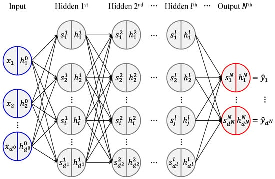
A DNN is a type of machine learning model that consists of multiple layers of interconnected nodes or neurons, each of which performs a specific function. The layers are arranged in a hierarchy, with each successive layer learning more complex features from the input data [53,54,55]. As illustrated in Figure 1, the general architecture of DNN consists of input, hidden, and output layers.

Figure 1. Architecture of deep neural network with $l$ hidden layers. $x$ and $y$ are the input and output of the deep neural network, and $s$ and $h$ are the input and output of each node, respectively.

An input column vector $\mathbf{x}={[x_1,x_2,\cdots ,x_{d^0}]}^{\mathrm{T}}$ and an output column vector $\mathbf{y}={[y_1,y_2,\cdots ,y_{d^N}]}^{\mathrm{T}}$ are given a dataset, where $d^{\left(0\right)}$ and $d^{\left(N\right)}$ are the length of the input and output, respectively. At this point, the output of the input neuron, $h_j^{\left(0\right)}$, is same as the $\mathbf{x}$. Accordingly, the input of $l$th layer, $s_j^{\left(l\right)}$, is obtained using $h_i^{(l-1)}$, combined with a column vector of weights, $w_{ji}^{\left(l\right)}$, and a bias, $b_j^{\left(l\right)}$ as follows:

$$s_j^{\left(l\right)}=w_{ji}^{\left(l\right),\mathrm{T}}{h}_i^{(l-1)}+b_j^{\left(l\right)}$$

(1)

where $w_{ji}^{\left(l\right)}={\left[w_{j1}^{\left(l\right)},w_{j2}^{\left(l\right)},\cdots ,w_{j{d}^{\left(l-1\right)}}^{\left(l\right)}\right]}^{\mathrm{T}}$ represents the weights affecting the $j$th neuron in the $l$th layer and all of the neurons in the $\left(l-1\right)$th layer and $b_j^{\left(l\right)}$ is the bias in the $l$th layer. Hereafter, the output of each neuron in the $l$th layer is obtained introducing an activation function, $h\left(·\right)$, as follows:

$$h_j^{\left(l\right)}=h\left(s_j^{\left(l\right)}\right)$$

(2)

where $h_j^{\left(l\right)}={\left[h_1^{\left(l\right)},h_2^{\left(l\right)},\cdots ,h_{d^{\left(l\right)}}^{\left(l\right)}\right]}^{\mathrm{T}}$ is the column vector of the output of the $j$th neuron in the $l$th layer with the length of $d^{\left(l\right)}$. In the hidden layers, the length of output vector, $d^{\left(l\right)}$, denotes the width or depth of the $l$th layer.

After a forward propagation by initializing the weights and calculating the predicted output $\widehat{\mathbf{y}}$ using Equations (1) and (2), the loss is calculated to perform backpropagation and optimize the weights. The most referenced loss function of mean square error (MSE) is employed in this study, The backpropagation is performed on the weights in the direction of minimizing the corresponding loss.

Meanwhile, the gradient-based optimization has been improved in several algorithms, including the adaptive gradient (AdaGrad) [70], the root mean square propagation (RMSprop) [71], and the adaptive moment estimation (Adam) [72]. To address the high-dimensionality and complexity inherent in reliability analysis problems, the Adam optimizer is used in this study due to its effectiveness and robustness against such challenges. The activation function presented in Equation (2) encodes the input into output of each neuron to determine whether the neuron should be activated or not based on the input, and to what extent it should be activated. In this study, two activation functions are utilized to deal with the nonlinearity of target reliability system, after investigations on the accuracy and stability. The Leaky ReLU which can address the vanishing gradient phenomenon is employed for the hidden layers [73]. In the last hidden layer, the output is activated using the hyperbolic tangent (tanh) function, which is nonlinearly defined and returns value ranging from −1 to 1. The combination of Leaky ReLU and tanh was adopted to balance gradient stability and bounded internal representation. Leaky ReLU mitigates vanishing gradient effects in deeper networks, while the tanh activation constrains the feature scale before the linear output layer, which was found to improve numerical stability near the limit state surface.

Before training the DNN model using aforementioned configuration, the input column vector is standardized using the mean and standard deviation of random variables. Those statistical properties are modeled and predefined in a reliability analysis problem. The number and width of hidden layers are experimentally adjusted through investigations on the accuracy and stability. To further improve the efficiency of training, mini-batch is employed with a size of 32 [74]. To address the problem of overfitting, early stopping of the training is adopted, and 90% and 10% of the dataset are set as the training set and validation set, respectively [75,76,77].

2.1.2. Weighted Sampling Method

Because the simple random sampling method selects experimental points without any predetermined criteria, there is a risk of bias in inference, which occurs when the selected samples are not representative of the population. Weighted sampling, on the other hand, is a technique where the probability of selecting a point is proportional to a weight assigned to that point [78]. Randomly selecting experimental points from the biased population can considerably degrade the performance of estimating a failure probability. To address this, in this study, the weighted sampling method proposed by Efraimidis and Spirakis [79] is utilized.

The weight coefficient of each sample point is determined in the following steps. Consider a population of $N$ points ${\mathbf{X}}^{\left(j\right)},(j=1,2,\cdots ,N)$, generated with respect to $n$ random variables. Then an $n$-dimensional hypercube can be defined with a side length of $X_l^n$ in the population space. The probability that a point is in the hypercube ($P_h^{\left(j\right)}$) can be obtained using the joint probability density function as follows:

$$P_h^{\left(j\right)}=f_{\mathbf{X}}\left({\mathbf{X}}^{\left(j\right)}\right)X_l^n$$

(3)

Assuming that the population points are subjected to a uniform distribution, the corresponding probability can be expressed using the range of the uniform distribution as follows:

$$P_h={\displaystyle \frac{1}{D^n}}{X}_l^n$$

(4)

where $D^n$ is the range of the uniform distribution. When the probabilities in Equations (3) and (4) are equal, a weight coefficient $w^{\left(j\right)}$ can be introduced as shown in Equation (5). This allows the probability of the experimental point selection to be subjected to the uniform distribution [79].

$$f_{\mathbf{X}}\left({\mathbf{X}}^{\left(j\right)}\right)X_l^n{w}^{\left(j\right)}={\displaystyle \frac{1}{D^n}}·X_l^n$$

(5)

With the weight coefficient generated, the weighted sampling is conducted as follows. First, generate a new random variable $u^{\left(j\right)},(j=1,2,\cdots ,N)$ subjected to uniform distribution with the lower and upper bounds of 0 and 1, respectively, where $N$ is the number of population points. Second, calculate the indexing value as shown in Equation (6).

$$I_v^{\left(j\right)}={\displaystyle \frac{\log \left(u^{\left(j\right)}\right)}{w^j}}$$

(6)

where $I_v^{\left(j\right)}$ is the indexing value of $j$th population point. Third, sort the population points according to the indexing value, and select the experimental points with the largest indexing value.

2.2. Proposed Active-Learning-Driven Deep Neural Network Meta Model

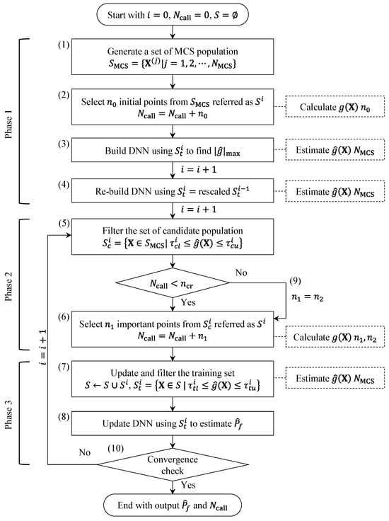
The proposed ALDNN meta model consists of three major phases: The first phase is about initial weighted sampling and rescaling of DNN. The second phase is about filtering candidate population and selecting of important experimental points; and the third phase is about removing noise and precise prediction by adding more important points. The algorithm of the proposed method is shown in Figure 2.

Figure 2. Flowchart of the proposed active-learning-driven DNN meta model algorithm comprising three phases.

2.2.1. Phase 1: Initial Sampling and Rescaling

Phase 1 steps include the following:

(1)

Start with $i=$ 0, where $i$ is the iteration number, and generate a set of MCS population ($S_{\mathrm{M}\mathrm{C}\mathrm{S}}$).

$$S_{\mathrm{M}\mathrm{C}\mathrm{S}}=\left\{{\mathbf{X}}^{\left(j\right)}|j=1,2,\cdots ,N_{\mathrm{M}\mathrm{C}\mathrm{S}}\right\}$$

(7)

(2)

Select $n_0$ initial points from $S_{\mathrm{M}\mathrm{C}\mathrm{S}}$ to build a set of selected experimental points ($S^i$). Here, $n_0$ is the number of initial samplings in phase 1, which is predetermined experimentally according to the complexity of the target system. The selected $n_0$ points are used to calculate the real value of limit state function. $n_0$ primarily determines the stability of early stage training by ensuring sufficient global coverage of the input space. The training set ($S_t^i$) is constructed using $S^i$, and calculate the corresponding real values of limit state function as follows:

$$S_t^i=\left\{\left({\mathbf{X}}^{\left(j\right)},{\mathbf{Y}}^{\left(j\right)}\right)|j=1,2,\cdots ,n_t\right\}$$

(8)

where ${\mathbf{X}}^{\left(j\right)}$ is the input matrix of the experimental points, ${\mathbf{Y}}^{\left(j\right)}$ is the output (i.e., real value of limit state function) vector of the experimental points, and $n_t$ is the number of training experimental points.

(3)

Build an initial DNN using the training set $S_t^i$. Based on the trained DNN, the value of $\widehat{g}\left(\mathbf{X}\right)$ is estimated for all population points, and ${\widehat{P}}_f$ in this initial iteration can be roughly obtained.

(4)

Re-build the DNN without updating using the rescaled $S_t^i$. The ${\mathbf{Y}}^{\left(j\right)}$ is normalized using ${\left|\widehat{g}\right|}_{\mathrm{m}\mathrm{a}\mathrm{x}}$ for rescaling and the estimation on $\widehat{g}\left(\mathbf{X}\right)$ is repeated.

$${\left|\widehat{g}\right|}_{\mathrm{m}\mathrm{a}\mathrm{x}}=\max \left[\begin{array}{c}\left\{\left|\widehat{g}\left(\mathit{X}\right)\right||\mathit{X}\in S_{\mathrm{M}\mathrm{C}\mathrm{S}}\right\}, \\ \left\{\left|g\left({\mathit{X}}^{\left(j\right)}\right)\right| | j=1,2,\cdots ,n_t\right\}\end{array}\right]$$

(9)

2.2.2. Phase 2: Filtering Candidate Population

Phase 2 steps include the following:

(5)

Filter the set of candidate population based on the feedback from the previous iteration. This process enables the meta model to actively select the important experimental points for the next training iteration.

$$S_c^i=\left\{\mathbf{X}\in S_{\mathrm{M}\mathrm{C}\mathrm{S}}|{\tau }_{cl}^i\le \widehat{g}(\mathbf{X})\le {\tau }_{cu}^i\right\}$$

(10)

where $S_c^i$ is the set of candidate population in $i$th iteration and ${\tau }_{cl}^i$ and ${\tau }_{cu}^i$ are the lower and upper thresholds for candidate population points in $i$th iteration that are defined as follows:

$${\tau }_{cl}^i=\left\{\begin{array}{c}-\infty , \hspace{0.17em}i<2\\ {\mu }_i\min \left[{\widehat{g}}^{i-1}\left(\mathbf{X}\right)\right], \hspace{0.17em}\hspace{0.17em}i=2\\ {\mu }_i{\tau }_{cl}^{i-1}, \hspace{0.17em}\hspace{0.17em}i>2\end{array}\right.$$

(11)

$${\tau }_{cu}^i=\left\{\begin{array}{c}\infty , \hspace{0.17em} i<2\\ {\mu }_i\max \left[{\widehat{g}}^{i-1}\left(\mathbf{X}\right)\right], \hspace{0.17em}\hspace{0.17em}\hspace{0.17em}\hspace{0.17em}\hspace{0.17em}i=2\\ {\mu }_i{\tau }_{cu}^{i-1}, \hspace{0.17em} i>2\end{array}\right.$$

(12)

where ${\mu }_i$ is the decreasing factor for candidate population threshold, which is determined through examinations. ${\mu }_i$ can be set as ${\mu }_i=$ 0.5 for $i\le$2 and ${\mu }_i=$0.8 for $i>$2, for example.

(6)

Select $n_1$ experimental points ($n_1<n_0$) from $S_c^i$ to build the set of selected experimental points ($S^i$). $n_1$ governs the refinement of the meta model near the limit state surface.

2.2.3. Phase 3: Removing Noise and Precise Prediction

Phase 3 includes the following:

(7)

The selected experimental points in $i$th iteration are added to the cumulative set of selected experimental points ($S$) as follows:

$$S=S\cup S^i$$

(13)

Meanwhile, the experimental points that are distant from the limit state surface are considered noise because they potentially weaken the performance of the meta model. Therefore, removing noise is conducted by filtering the cumulative set of experimental points as follows:

$$S_t^i=\left\{\mathbf{X}\in S|{\tau }_{tl}^i\le \widehat{g}(\mathbf{X})\le {\tau }_{tu}^i\right\}$$

(14)

$${\tau }_{tl}^i=\left\{\begin{array}{c}{\gamma }_i\min \left[{\widehat{g}}^{i-1}\left(\mathbf{X}\right)\right], i=2\\ {\gamma }_i{\tau }_{tl}^{i-1}, i>2\end{array}\right.$$

(15)

$${\tau }_{tu}^i=\left\{\begin{array}{c}{\gamma }_i\max \left[{\widehat{g}}^{i-1}\left(\mathbf{X}\right)\right], i=2\\ {\gamma }_i{\tau }_{tu}^{i-1}, i>2\end{array}\right.$$

(16)

where ${\tau }_{tl}^i$ and ${\tau }_{tu}^i$ are the lower and upper thresholds for training set in $i$th iteration and ${\gamma }_i$ is the decreasing factor for removing noise. In this study, ${\gamma }_i$ is set as 0.9.

(8)

Update the DNN using the filtered training set $S_t^i$ to estimate $\widehat{g}\left(\mathbf{X}\right)$ and ${\widehat{P}}_f$.

(9)

If the cumulative $N_{\mathrm{c}\mathrm{a}\mathrm{l}\mathrm{l}}$ exceeds a specific criterion ($n_{\mathrm{c}\mathrm{r}}$), select $n_2$ experimental points ($n_2<n_1$) instead of $n_1$. In this study, $n_{\mathrm{c}\mathrm{r}}=2n_0$ is considered through examinations.

(10)

The relative error of estimated failure probability, denoted as ${\epsilon }_{{\widehat{P}}_f}$, is monitored to assess convergence. The stopping criterion is defined based on the relative change in the estimated failure probability between successive iterations, which indicates stabilization of the meta model near the limit state surface. In this study, the relative error tolerance is set to 0.005, and the maximum number of iterations is set to 30.

3. Results

3.1. Benchmark Problems

To evaluate the performance of the ALDNN meta model, the most frequently referenced benchmark problems were employed. These problems serve as verification procedures to ensure improved efficiency while maintaining accuracy. Reliability analysis results include the failure probability ($P_f$), the reliability index ($\beta$), and the number of limit state function calls ($N_{\mathrm{c}\mathrm{a}\mathrm{l}\mathrm{l}}$), compared with previous studies. For fair comparison, identical random seeds were used in each benchmark case to eliminate stochastic bias in sampling. It should be noted that, because the computer specification and programming code used in each of the literature are different, a direct comparison of solution time was not feasible [69]. Therefore, the solution time was compared for the proposed meta model and the MCS performed in this study.

3.1.1. Series System with Four Branches

The first benchmark problem is a series system consisting of two-dimensional random variables with multiple failure modes [43,66,80,81,82,83]. This problem illustrates how the proposed method works in a two-variable case, which can be easily visualized and understood. The limit state function is defined as Equation (17).

$$g\left(X_1,X_2\right)=\mathrm{m}\mathrm{i}\mathrm{n}\left\{\begin{array}{c}\begin{array}{c}3+0.1{(X_1-X_2)}^2-{\displaystyle \frac{X_1-X_2}{\sqrt{2}}},\\ 3+0.1{(X_1-X_2)}^2+{\displaystyle \frac{X_1-X_2}{\sqrt{2}}},\end{array}\\ \begin{array}{c}\left(X_1-X_2\right)+{\displaystyle \frac{k}{\sqrt{2}}},\\ \left(X_2-X_1\right)+{\displaystyle \frac{k}{\sqrt{2}}}\end{array}\end{array}\right.$$

(17)

where $X_1$ and $X_2$ are the random variables subjected to standard normal distribution and $k$ is a constant that is set to six and seven according to the literature [66]. The meta model configuration settings for this problem are as follows: The number and width of hidden layers are set to 4 and 200, respectively. $n_0$, $n_1$ and $n_2$ are set to 30, 10 and 2, respectively; and $n_{\mathrm{c}\mathrm{r}}$ is set to $2n_0$. The size of MCS population is set to 1 $\times$ 10⁶ in accordance with the literature.

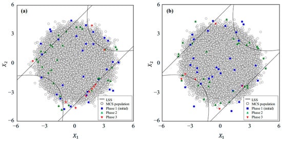
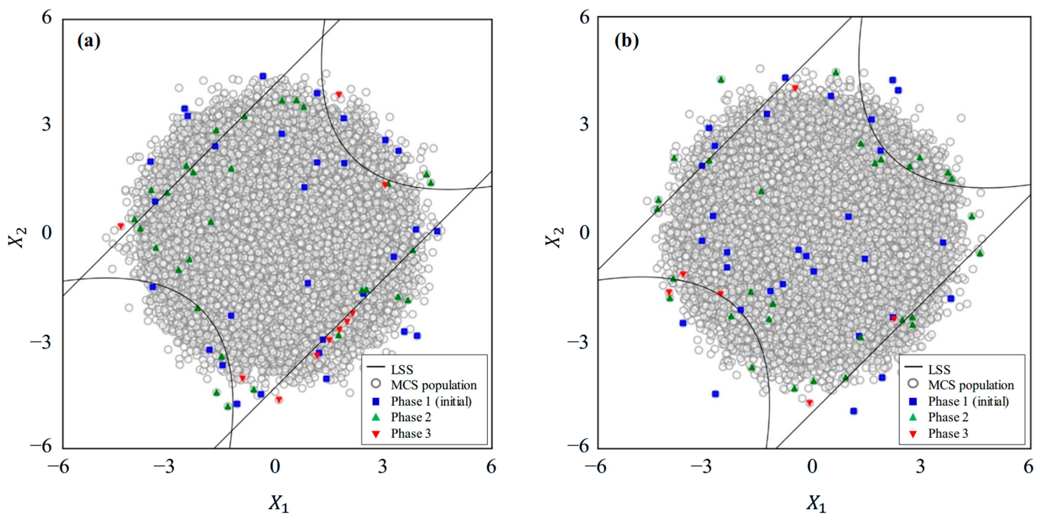
Figure 3 presents the selected experimental points for the problem with $k =$ 6 and 7. The 30 initial points selected in phase 1 were uniformly distributed in the MCS population space, marked in blue in Figure 3. In the second phase, a total of 30 experimental points was selected, marked in red, getting closer to the limit state surface. In the third phase, the iteration converged after adding a total of 10 and 6 points for $k =$ 6 and 7 cases, respectively.

Figure 3. Selected experimental points using an active-learning-driven DNN meta model for the series system with four branches. (a) $k =$ 6 and (b) $k =$7.

The reliability analysis results of MCS and different methods are presented in Table 1 and Table 2. The estimation of $P_f$ and $\beta$ using the proposed method was in great agreement with those using the MCS. However, while the MCS required 1 $\times$ 10⁶ calls of limit state function, only 70 calls were required in the proposed method. For the problem with $k =$ 7, the ${\epsilon }_{\beta }$ of the proposed method was 0.141% with only 66 calls of limit state function. Compared to other methods, a smaller relative error was calculated overall while requiring fewer $N_{\mathrm{c}\mathrm{a}\mathrm{l}\mathrm{l}}$. For the $k =$ 6 case, the methods requiring the least $N_{\mathrm{c}\mathrm{a}\mathrm{l}\mathrm{l}}$ were the directional sampling (DS) and the importance sampling (IS) combined with neural network proposed by [43]. However, the DS method showed poor estimation when the limit state surface had a radial shape, i.e., $k =$ 7, as in Table 2 [43,67].

Table 1. Reliability analysis results for the series system with four branches ($k =$ 6) compared by methods [43,66,67,69].

Method	Number of g Calls, Ncall	Failure Probability, Pf	Reliability Index, β	Relative Error of β, εβ (%)
MCS	$1 \times$ 106	$4.425 \times$ 10−3	2.617	-
Proposed ALDNN Meta Model	70	$4.467 \times$ 10−3	2.614	0.115
Directional Sampling (DS)	52	$4.500 \times$ 10−3	2.612	0.191
DS + Response Surface	1745	$5.000 \times$ 10−3	2.578	1.490
DS + Spline	145	$2.400 \times$ 10−3	2.820	7.757
DS + Neural Network	165	$4.100 \times$ 10−3	2.644	1.032
Importance Sampling (IS)	1469	$4.900 \times$ 10−3	2.583	1.299
IS + Response Surface	1375	$4.500 \times$ 10−3	2.612	0.191
IS + Spline	428	$4.500 \times$ 10−3	2.612	0.191
IS + Neural Network	52	$5.700 \times$ 10−3	2.530	3.324
AK-MCS + U	126	$4.416 \times$ 10−3	2.618	0.038
AK-MCS + EFF	124	$4.412 \times$ 10−3	2.618	0.038
DNN by [67]	80	$4.414 \times$ 10−3	2.619	0.076
DNN by [69]	133	$4.409 \times$ 10−3	2.619	0.076

Table 2. Reliability analysis results for the series system with four branches ($k =$ 7) compared by methods [66,67,84].

Method	Number of g Calls, Ncall	Failure Probability, Pf	Reliability Index, β	Relative Error of β, εβ (%)
MCS	$1 \times$ 106	$2.231 \times$ 10−3	2.844	-
Proposed ALDNN Meta Model	66	$2.253 \times$ 10−3	2.840	0.141
Directional Sampling (DS)	9192	$2.600 \times$ 10−3	2.794	1.758
DS + Response Surface	830	$1.000 \times$ 10−3	3.090	8.650
DS + Spline	107	$1.000 \times$ 10−3	3.090	8.650
DS + Neural Network	67	$1.000 \times$ 10−3	3.090	8.650
DS + Ordinary Kriging	107	$1.500 \times$ 10−3	2.978	4.712
Importance Sampling (IS)	4750	$2.200 \times$ 10−3	2.848	0.141
IS + Response Surface	3877	$2.000 \times$ 10−3	2.878	1.195
IS + Spline	724	$2.000 \times$ 10−3	2.878	1.195
IS + Neural Network	125	$2.900 \times$ 10−3	2.759	2.989
IS + Ordinary Kriging	146	$2.000 \times$ 10−3	2.878	1.195
AK-MCS + U	96	$2.233 \times$ 10−3	2.843	0.035
AK-MCS + EFF	101	$2.232 \times$ 10−3	2.843	0.035
DNN by [67]	70	$2.188 \times$ 10−3	2.850	0.211

Meanwhile, the active learning reliability method combining Kriging and MCS (AK-MCS) with two different learning functions (U and EFF) by [66] showed the highest accuracy (0.038% of ${\epsilon }_{\beta }$) for the $k =$ 6 case. Additionally, the methods by [67,69] that utilized deep neural network also showed high accuracy. However, the $N_{\mathrm{c}\mathrm{a}\mathrm{l}\mathrm{l}}$ of these methods were greater than that of the proposed method, showing that the performance of the proposed method has been further improved in terms of efficiency.

For the $k =$ 7 case (Table 2), the method from the literature requiring the least $N_{\mathrm{c}\mathrm{a}\mathrm{l}\mathrm{l}}$ was the DS combined with neural network by [84]; however, it showed the worst accuracy (67 $N_{\mathrm{c}\mathrm{a}\mathrm{l}\mathrm{l}}$ and 8.650% of ${\epsilon }_{\beta }$). The IS method in this case could demonstrate great accuracy; however, it required a large size of $N_{\mathrm{c}\mathrm{a}\mathrm{l}\mathrm{l}}$ (4750 $N_{\mathrm{c}\mathrm{a}\mathrm{l}\mathrm{l}}$ and 0.141% of ${\epsilon }_{\beta }$). The aforementioned AK-MCS methods by [66] and the deep learning method by [69] also showed a satisfactory performance. However, in this case as well, the proposed meta model method was evaluated to be more effective when considering both accuracy and efficiency.

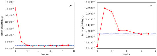
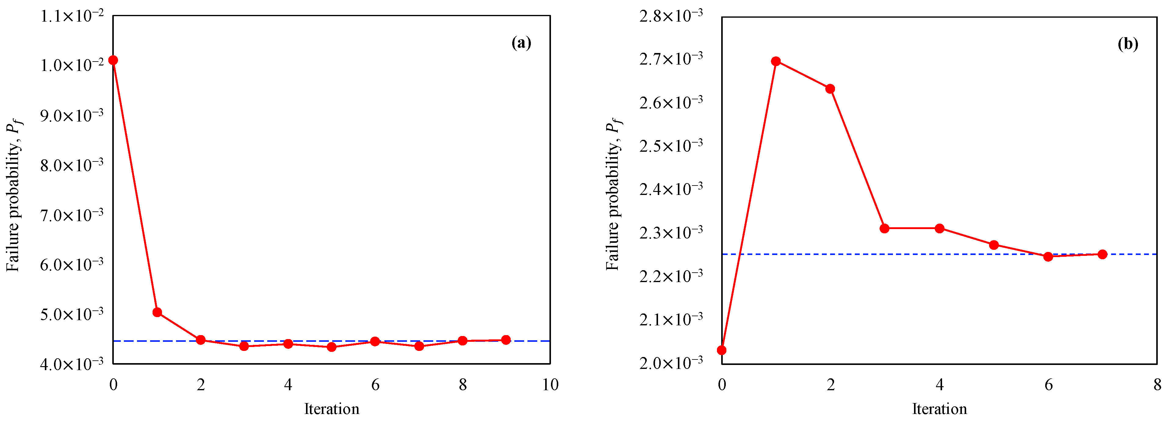
The solution time for MCS and the proposed method was 4.859 and 430.790 s, respectively, in the $k =$ 6 case and 4.843 and 416.431 s, respectively, in the $k =$ 7 case. Because the limit state function of this problem was mathematically explicit, the computational cost to directly calculate the value of the function was insignificant. Therefore, the proposed method, which trains the DNN through a multi-phase, threshold-based active learning framework, required more solution time for this simple system. The convergence history of the estimated $P_f$ using the ALDNN meta model is shown in Figure 4.

Figure 4. Failure probability convergence according to iteration in the series system with four branches problem. (a) k = 6 and (b) k = 7. The blue dotted line represents the converged failure probability.

3.1.2. Dynamic Response of a Nonlinear Oscillator

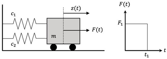
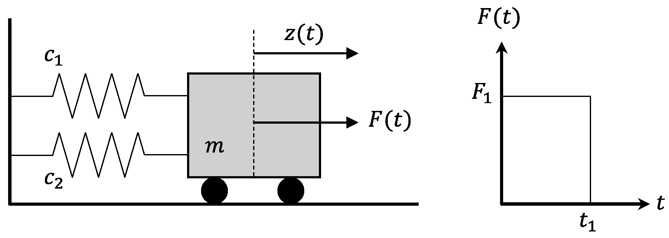
To test the performance of the proposed method in solving a nonlinear problem, a dynamic response of nonlinear oscillator problem is employed [37,43,66,81,83,85]. The graphical system definition of the problem is shown in Figure 5, and the limit state function is defined as Equation (18).

$$g\left(m,c_1,c_2,r,F_1,t_1\right)=3r-\left|z_{\mathrm{m}\mathrm{a}\mathrm{x}}\right|=3r-\left|{\displaystyle \frac{2F_1}{m{{\omega }_0}^2}}\mathrm{s}\mathrm{i}\mathrm{n}\left({\displaystyle \frac{{\omega }_0{t}_1}{2}}\right)\right|$$

(18)

where $m$ is the mass of the system, $c_1$ and $c_2$ are the stiffness of the springs, $r$ is the displacement, and $F_1$ and $t_1$ represent the rectangular load pulse. $z_{max}$ is the maximum displacement response of the oscillator, and ${\omega }_0=\sqrt{(c_1+c_2)/m }$. The statistical properties of the random variables are listed in Table 3.

Figure 5. System definition of nonlinear oscillator.

Table 3. Statistical properties of random variables for the nonlinear oscillator.

Random Variable	Mean	Standard Deviation	Distribution
m	1.0	0.05	Normal
c1	1.0	0.10	Normal
c2	0.1	0.01	Normal
r	0.5	0.05	Normal
F1	1.0	0.20	Normal
t1	1.0	0.20	Normal

The meta model configuration settings for this problem are as follows: The number and width of hidden layers are set to 2 and 150, respectively. $n_0$, $n_1$ and $n_2$ are set to 25, 2 and 1, respectively; and $n_{\mathrm{c}\mathrm{r}}$ is set to $2n_0$. Because the target $P_f$ is greater than that of the previous series system problem, the number of selected points in each phase and the width of hidden layers are adjusted through experiments. The size of MCS population is set to 7 $\times$ 10⁴ according to the literature.

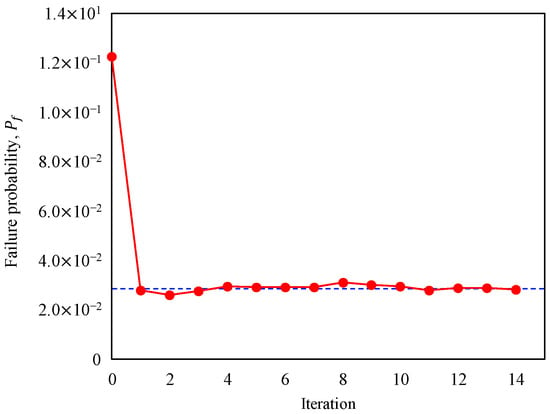
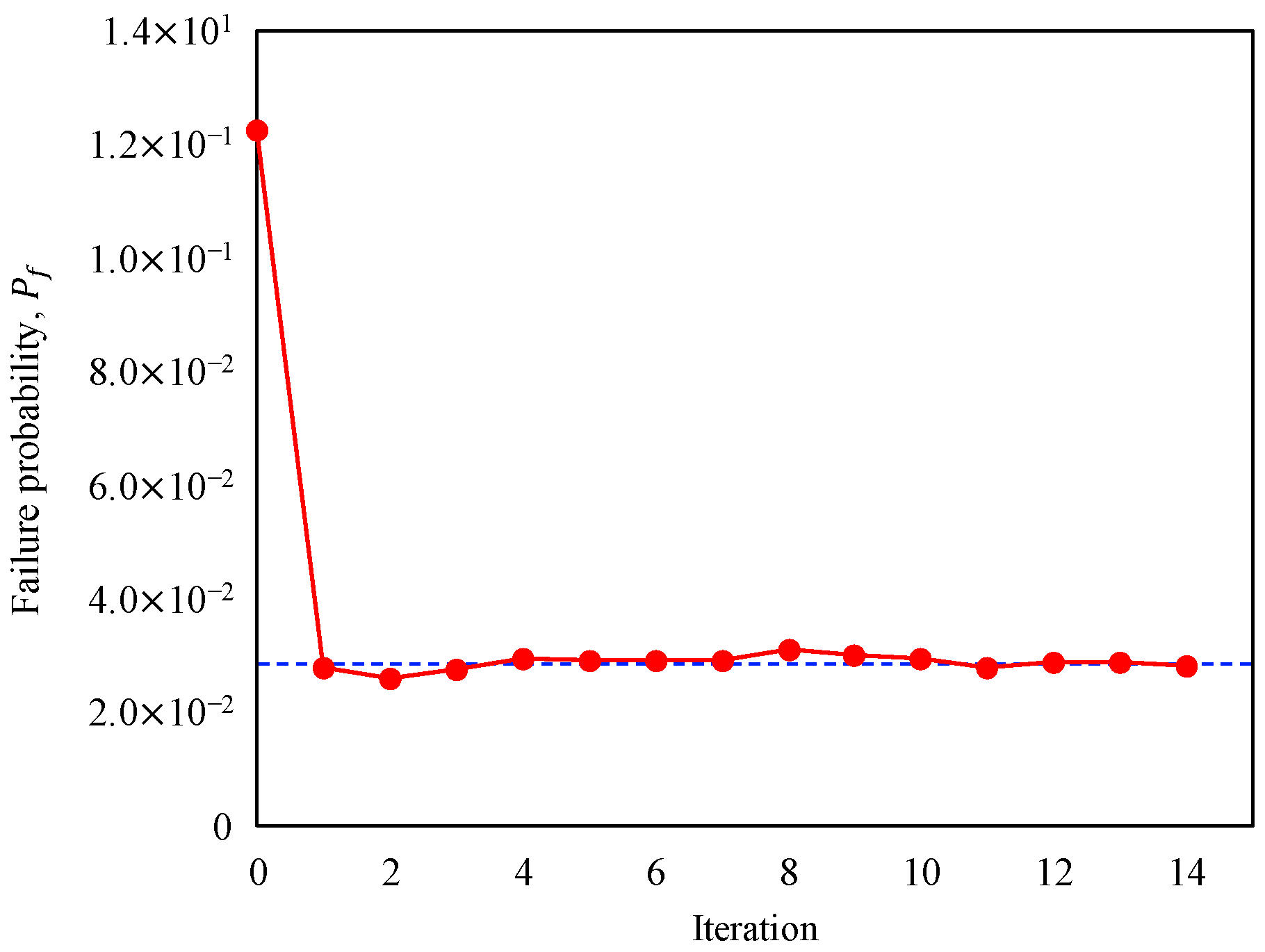
Table 4 shows the results of the reliability analysis for this nonlinear problem. The estimated $P_f$ by the proposed meta model was in great agreement with those by the MCS, requiring a substantially small size of $N_{\mathrm{c}\mathrm{a}\mathrm{l}\mathrm{l}}$. The proposed method achieved an ${\epsilon }_{\beta }$ of 0.000% with only 52 of $N_{\mathrm{c}\mathrm{a}\mathrm{l}\mathrm{l}}$. The computational solution time for MCS and the proposed method was 0.281 and 168.827 s, respectively. The overall time consumed was reduced compared to the first problem due to the lower complexity of the system. However, the time of the proposed method was still much longer than that of MCS. The convergence history of the estimated $P_f$ is shown in Figure 6.

Table 4. Reliability analysis results for the dynamic response of nonlinear oscillator compared by methods [43,66,67,69].

Method	Number of g Calls, Ncall	Failure Probability, Pf	Reliability Index, β	Relative Error of β, εβ (%)
MCS	7 × 104	2.820 × 10−2	1.908	-
Proposed ALDNN Meta Model	52	2.820 × 10−2	1.908	0.000
Directional Sampling (DS)	1281	3.500 × 10−2	1.812	5.031
DS + Response Surface	62	3.400 × 10−2	1.825	4.350
DS + Spline	76	3.400 × 10−2	1.825	4.350
DS + Neural Network	86	2.800 × 10−2	1.911	0.157
Importance Sampling (IS)	6144	2.700 × 10−2	1.927	0.996
IS + Response Surface	109	2.500 × 10−2	1.960	2.725
IS + Spline	67	2.700 × 10−2	1.927	0.996
IS + Neural Network	68	3.100 × 10−2	1.866	2.201
AK-MCS + U	58	2.834 × 10−2	1.906	0.105
AK-MCS + EFF	45	2.851 × 10−2	1.903	0.262
DNN by [67]	35	2.836 × 10−2	1.905	0.157
DNN by [69]	77	2.829 × 10−2	1.907	0.052

Figure 6. Failure probability convergence according to iteration in the nonlinear oscillator problem. The blue dotted line represents the converged failure probability.

3.1.3. High-Dimensional Problem

The problem designed by Rackwitz [3], which involves a large number of random variables [11] is employed to test the performance in solving a high-dimensional problem. The limit state function is shown as Equation (19).

$$g\left(X_1,\cdots ,X_n\right)=\left(n+3\sigma \sqrt{n}\right)-\sum _{i=1}^n{X}_i$$

(19)

where $X_i$ is the random variables and $n$ is the number of random variables. The number of random variables is set to 40 and 100 in accordance with the literature. The random variables are subjected to a lognormal distribution with unit mean and standard deviation of $\sigma =$0.2. The model configuration settings for this problem are as follows: For the $n =$ 40 case, one hidden layer with a width of 40 is set. $n_0$, $n_1$ and $n_2$ are set to 50, 2 and 1, respectively, considering the linearity and the number of random variables of the target system. For the $n =$ 100 case, one hidden layer with a width of 100 is set; $n_0$, $n_1$ and $n_2$ are set to 115, 2 and 1, respectively. Because of its apparent linearity, the architecture of hidden layer and the number of selecting points in each phase are adjusted through experiments. The size of MCS population is set to 3 $\times$ 10⁵ according to the literature and the target $P_f$.

Table 5 presents the results of reliability analysis for the high-dimensional problem conducted through various methods. As a result, the $P_f$ estimated by the proposed meta model agreed with those by the MCS, requiring substantially small size of $N_{\mathrm{c}\mathrm{a}\mathrm{l}\mathrm{l}}$. When compared to other methods, the proposed meta model method showed the smallest relative error while requiring the least $N_{\mathrm{c}\mathrm{a}\mathrm{l}\mathrm{l}}$. In this high-dimensional problem, the iteration of ALDNN meta model converged at the start of the second phase. In the initial iteration, the first estimation of the $P_f$ was fairly accurate. The computational solution time for MCS and the proposed method is presented in Table 6. The solution time of the proposed method was still longer than that of MCS. At this time, it was observed that the time increased as the complexity of the system increased.

Table 5. Reliability analysis results for the high-dimensional problem compared by methods [66,67].

Method	Number of g Calls, Ncall	Failure Probability, Pf	Reliability Index, β	Relative Error of β, εβ (%)
$n =$ 40
MCS	$3 \times$ 105	$1.863 \times$ 10−3	2.900	-
Proposed ALDNN meta model	52	$1.867 \times$ 10−3	2.900	0.000
AK-MCS + U	112	$1.813 \times$ 10−3	2.909	0.310
AK-MCS + EFF	124	$1.813 \times$ 10−3	2.909	0.310
DNN by [67]	62	$1.810 \times$ 10−3	2.910	0.345
$n =$ 100
MCS	$3 \times$ 105	$1.623 \times$ 10−3	2.943	-
Proposed ALDNN meta model	117	$1.623 \times$ 10−3	2.943	0.000
AK-MCS + U	153	$1.647 \times$ 10−3	2.939	0.136
AK-MCS + EFF	167	$1.647 \times$ 10−3	2.939	0.136
DNN by [67]	122	$1.630 \times$ 10−3	2.942	0.034

Table 6. Comparison of solution times for high-dimensional problem with increasing complexity.

Method	Complexity of System		Increasing Rate
	$\mathit{n} =$ 40	$\mathit{n} =$ 100	150.00%
MCS	3.016 s	7.720 s	156.97%
Proposed ALDNN meta model	179.547 s	204.735 s	14.02%

3.1.4. Speed Reducer Shaft

The last benchmark problem is employed to consider various distributions of random variables [11,81]. The limit state function is presented as follows:

$$g\left(D,L,S,F,T\right)=S-{\displaystyle \frac{32}{\pi D^3}}\sqrt{{\displaystyle \frac{L^2{F}^2}{16}}}+T^2$$

(20)

where $D$ is the diameter of the shaft, $L$ is the length of the shaft, $S$ represents the material strength, $F$ represents the external force, and $T$ represents the external torque. The statistical properties of the random variables are listed in Table 7, with various types of distribution including normal, uniform, and Gumbel.

Table 7. Statistical properties of random variables for the speed reducer shaft.

Random Variable	Unit	Mean	Standard Deviation	Distribution
$D$	mm	39	0.1	Normal
$L$	mm	400	0.1	Normal
$S$	MPa	70 *	80 **	Uniform
$F$	N	1500	350	Gumbel
$T$	$\mathrm{N}·$mm	250,000	35,000	Normal

* The lower bound of the uniform distribution. ** The upper bound of the uniform distribution.

The meta model configuration settings for this problem are as follows: The number and width of hidden layers are set to 2 and 200, respectively. $n_0$, $n_1$ and $n_2$ are set to 60, 10 and 2, respectively; and $n_{\mathrm{c}\mathrm{r}}$ is set to $2n_0$ as presented previously. The size of MCS population is set to 1 $\times$ 10⁶ according to the literature and the target $P_f$.

Table 8 presents the results of the reliability analysis for the speed reducer shaft by various methods. The $P_f$ estimated by the proposed meta model agreed with those by the MCS, requiring a small size of $N_{\mathrm{c}\mathrm{a}\mathrm{l}\mathrm{l}}$. In the analytical methods such as the FORM and the SORM, the accuracy of the estimation was considerably poor. The first-order saddlepoint approximation (FOSPA) by [11] and the sequential surrogate reliability method (SSRM) by [81] showed the least $N_{\mathrm{c}\mathrm{a}\mathrm{l}\mathrm{l}}$. However, they failed to estimate the $P_f$ accurately with large relative errors. Meanwhile, the DNN model by [67] could conduct a fairly accurate reliability analysis; however, the efficiency was slightly lower than the proposed method in this study.

Table 8. Reliability analysis results for the speed reducer shaft compared by methods [11,69,81].

Method	Number of g Calls, Ncall	Failure Probability, Pf	Reliability Index, β	Relative Error of β, εβ (%)
MCS	$1 \times$ 106	$7.620 \times$ 10−4	3.170	-
Proposed ALDNN meta model	126	$7.590 \times$ 10−4	3.171	0.032
FORM	1472	$7.007 \times$ 10−7	4.825	52.208
SORM	1514	$4.358 \times$ 10−7	4.919	55.174
FOSPA	102	$6.175 \times$ 10−4	3.231	1.924
SSRM	44	$7.520 \times$ 10−3	2.431	23.312
DNN by [69]	137	$7.831 \times$ 10−4	3.162	0.252

The solution time for the MCS and the proposed method was 3.781 and 534.289 s, respectively, showing the longest time consumed among the benchmark problems due to its rare probability. Figure 7 shows the convergence history of the estimated $P_f$ using the ALDNN meta model.

Figure 7. Failure probability convergence according to iteration in the speed reducer shaft problem. The blue dotted line represents the converged failure probability.

3.2. Finite-Element-Method-Based Implicit Problems

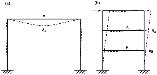
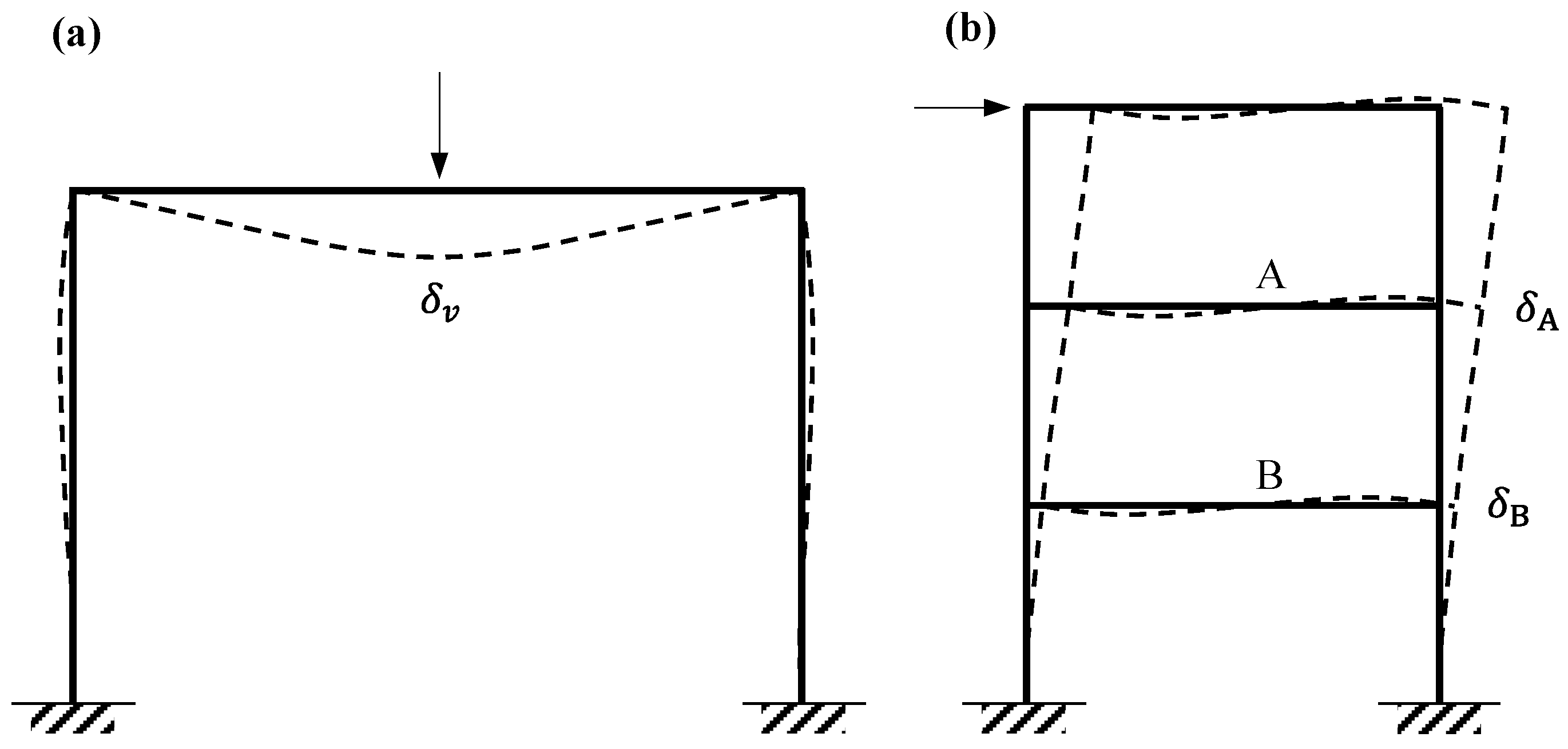
The applicability of the proposed ALDNN meta model is verified using structural reliability problems in which the limit states are implicitly defined. The limit state function $g\left(\mathbf{X}\right)$ cannot be expressed mathematically in terms of the random variables ($\mathbf{X}$) due to its implicitness and high complexity of its structural system. Therefore, the finite element method (FEM) analysis is utilized to calculate the structural response of limit state function. In strict terms, it is difficult to specify the limit state of a structure because the behavior and characteristics of structure are diverse. Therefore, instead of explicitly specifying the limit state of structure, a serviceability limit state presented in the design code is applied. The Korean steel structure design code [86] presents the limit of vertical deflection and story drift for frame structure as follows:

$${\delta }_v\le {\displaystyle \frac{l}{300}} (\mathrm{m})$$

(21)

$${\delta }_h^{\prime }\le 0.01 \left(\mathrm{m}\right)$$

(22)

where ${\delta }_v$ is the vertical deflection, $l$ is the span of the beam, and ${\delta }_h^{\prime }$ is the horizontal story drift. Figure 8 depicts the deformation of a frame structure showing the vertical deflection and the horizontal story drift. As shown in Figure 8b, the story drift of floor A is calculated as the difference between the horizontal displacements of the adjacent floors, as presented in Equation (23).

$${\delta }_h^{\prime }={\delta }_{\mathrm{A}}-{\delta }_{\mathrm{B}}$$

(23)

where ${\delta }_{\mathrm{A}}$ and ${\delta }_{\mathrm{B}}$ are the horizontal displacements of floors A and B, respectively. Utilizing the predefined limit state about the deformation, the limit state function can be constructed as follows:

$$g\left(\mathbf{X}\right)={\delta }_{\mathrm{l}\mathrm{i}\mathrm{m}\mathrm{i}\mathrm{t}}-FEM\left(\mathbf{X}\right)$$

(24)

where ${\delta }_{\mathrm{l}\mathrm{i}\mathrm{m}\mathrm{i}\mathrm{t}}$ is the limit (or allowable) deflection or story drift, which is defined according to the structural system. $FEM(·)$ denotes the response of the linear FEM analysis with $\mathbf{X}$ as input, which returns deflection or story drift depending on the configuration of the problem.

Figure 8. Deformation of frame. (a) Vertical deflection and (b) horizontal displacement of floor.

3.2.1. 2-Bay Planar Frame Under Vertical Load

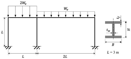
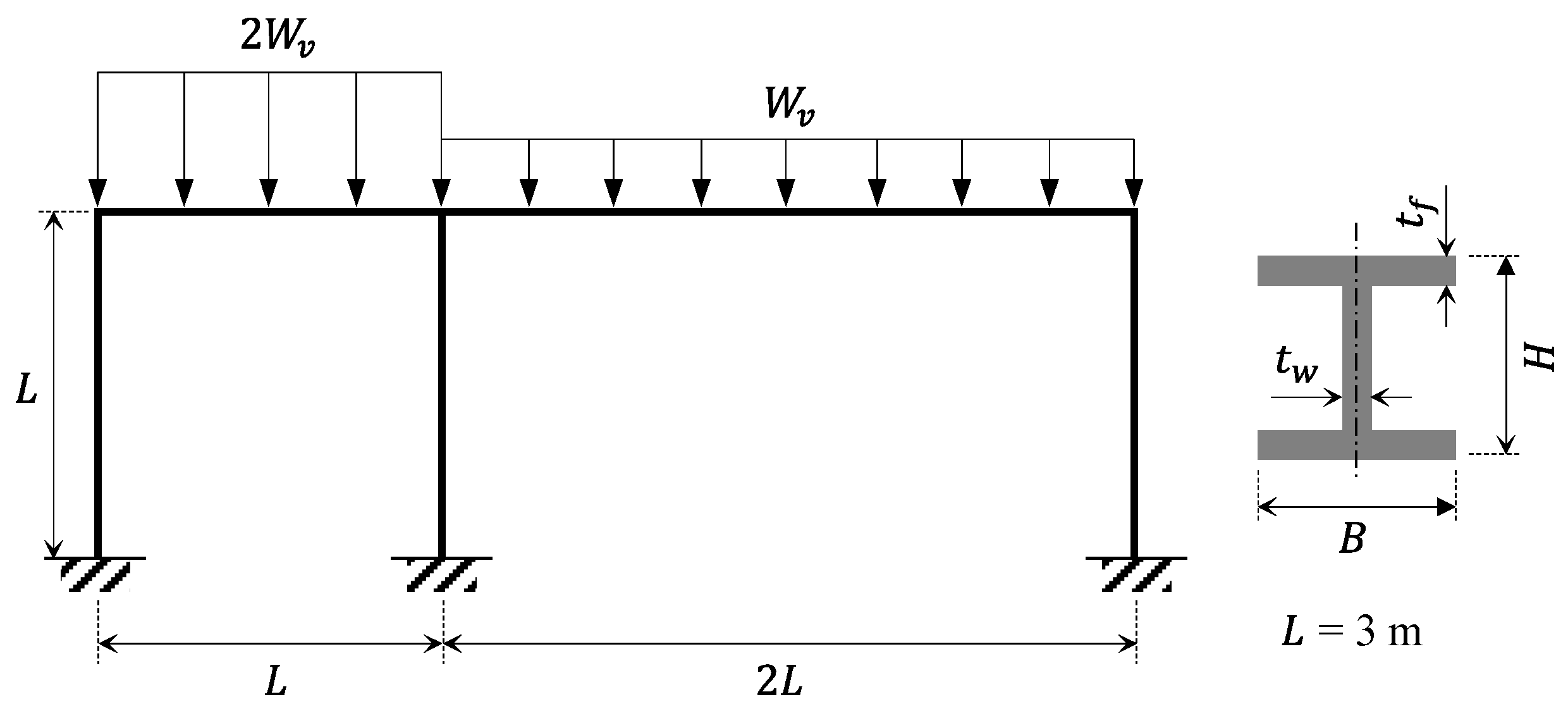
In the first FEM-based problem, a planar frame with 2-bay is employed as shown in Figure 9. To quantify the uncertainty in structural design, six parameters are modeled as input random variables. Firstly, the cross-sectional specification of H-beam is set as design random variables: the height of H-beam ($H$), the width of H-beam ($B$), and the thickness of web ($t_w$) and flange ($t_f$). Secondly, to consider the uncertainty of material property, the elastic modulus ($E$) is set as a random variable. In addition, to consider the uncertainty in external load, the distributed vertical load ($W_v$) is modeled as a random variable.

Figure 9. Configuration of 2-bay planar frame and the cross-sectional specifications of H-beam.

Based on previous investigations, the statistical properties of random variables are determined. Especially, the coefficient of variation (CoV) of the variables, which is the most frequently used tool for quantifying variability [87,88,89,90], is set according to the literature. The CoV, also known as the normalized standard deviation, is calculated by dividing the standard deviation ($\sigma$) by the mean ($\mu$) of random variable:

$$\mathrm{C}\mathrm{o}\mathrm{V}={\displaystyle \frac{\sigma }{\mu }}$$

(25)

For the cross-sectional definition, the lognormal or normal distribution and the CoV ranging from 0.013 to 0.036 [88,91,92] and from 0.012 to 0.029 [93,94,95,96] have been reported. For the elastic modulus, the CoV ranging from 0.042 to 0.058 and the normal distribution has been reported in previous studies [89,97,98]. The dead load variable is set to be subjected to a normal distribution with CoV of 0.1, as presented in Eurocode and US standard [98,99]. Based on the literature, the detailed statistical properties of the random variables are listed in Table 9.

Table 9. Statistical properties of random variables for the 2-bay planar frame.

Random Variable	Unit	Mean	Standard Deviation	Distribution
$H$	m	0.1	0.02	Lognormal
$B$	m	0.1	0.02	Lognormal
$t_w$	m	0.006	0.02	Lognormal
$t_f$	m	0.008	0.02	Lognormal
$E$	N/m2	$210 \times$ 109	0.05	Normal
$W_v$	N/m	2500	0.10	Normal

In this problem, the limit state function in Equation (24) can be modified considering the vertical deflection as follows:

$$g\left(\mathbf{X}\right)={\delta }_{v,\mathrm{l}\mathrm{i}\mathrm{m}\mathrm{i}\mathrm{t}}-FEM\left(\mathbf{X}\right)\left(\mathrm{m}\right)$$

(26)

where ${\delta }_{v, \mathrm{l}\mathrm{i}\mathrm{m}\mathrm{i}\mathrm{t}}=$ 6/300 (m) is the limit deflection according to Equation (21) and $FEM\left(\mathbf{X}\right)$ denotes the maximum deflection according to the results of FEM analysis. The meta model configuration settings for this problem are as follows: The number and width of hidden layers are set to 4 and 200, respectively. $n_0$, $n_1$ and $n_2$ are set to 80, 10 and 2, respectively; and $n_{\mathrm{c}\mathrm{r}}$ is set to $2n_0$, considering the complexity of the target system. The size of MCS population is set to 1 $\times$ 10⁵ considering the expected $P_f$.

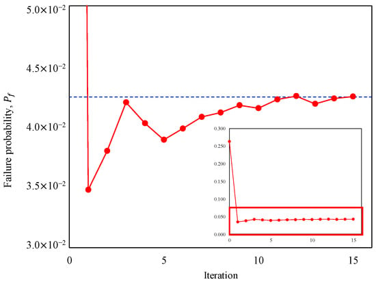
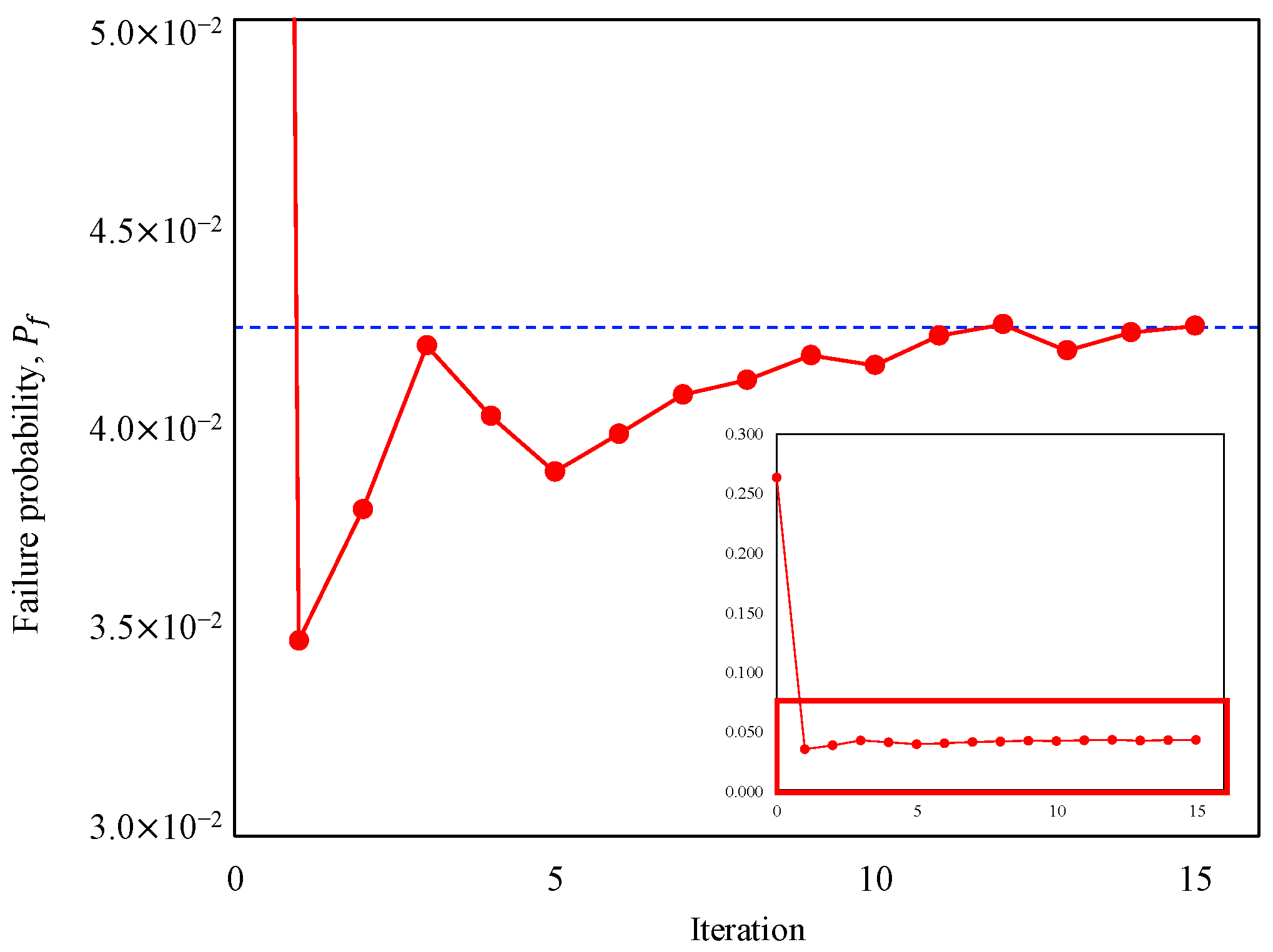
Table 10 shows the reliability analysis results for the 2-bay planar frame. It should be noted that the analytical methods such as FORM or SORM were completely not applicable to this problem because the limit state is implicitly defined. The ALDNN meta model calculated the $P_f$ as 4.248 $\times$ 10⁻², which was in great agreement with the solution by MCS. However, the $N_{\mathrm{c}\mathrm{a}\mathrm{l}\mathrm{l}}$ of the proposed method was only 172, while that of MCS was 1 × 10⁵, meaning that 172 and 1 × 10⁵ of FEM analyses were conducted in both methods, respectively.

Table 10. Results of reliability analysis for the 2-bay planar frame.

Method	Number of g Calls, Ncall	Failure Probability, Pf	Reliability Index, β	Relative Error of β, εβ (%)	Solution Time (s)
MCS	$1 \times$ 105	$4.208 \times$ 10−2	1.727	-	413.484
ALDNN meta model	172	$4.248 \times$ 10−2	1.723	0.231	423.156

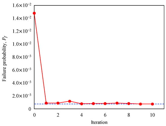
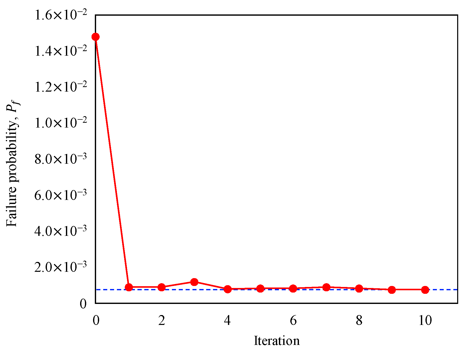
In this problem, the computational cost for a single call of $g\left(\mathbf{X}\right)$ was higher than those of the previous benchmark problems due to the increased complexity. Accordingly, the solution time in the proposed method exhibited no significant difference in comparison with that in the MCS. The solution time was still longer in the deep learning method, as the computational cost for $g\left(\mathbf{X}\right)$ calculation was not that substantial in this problem. The history of iteration convergence is plotted in Figure 10.

Figure 10. Failure probability convergence according to iteration in the 2-bay planar frame problem. The blue dotted line represents the converged failure probability.

3.2.2. 6-Story Space Frame with Lateral Load

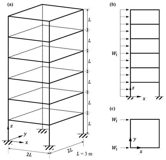
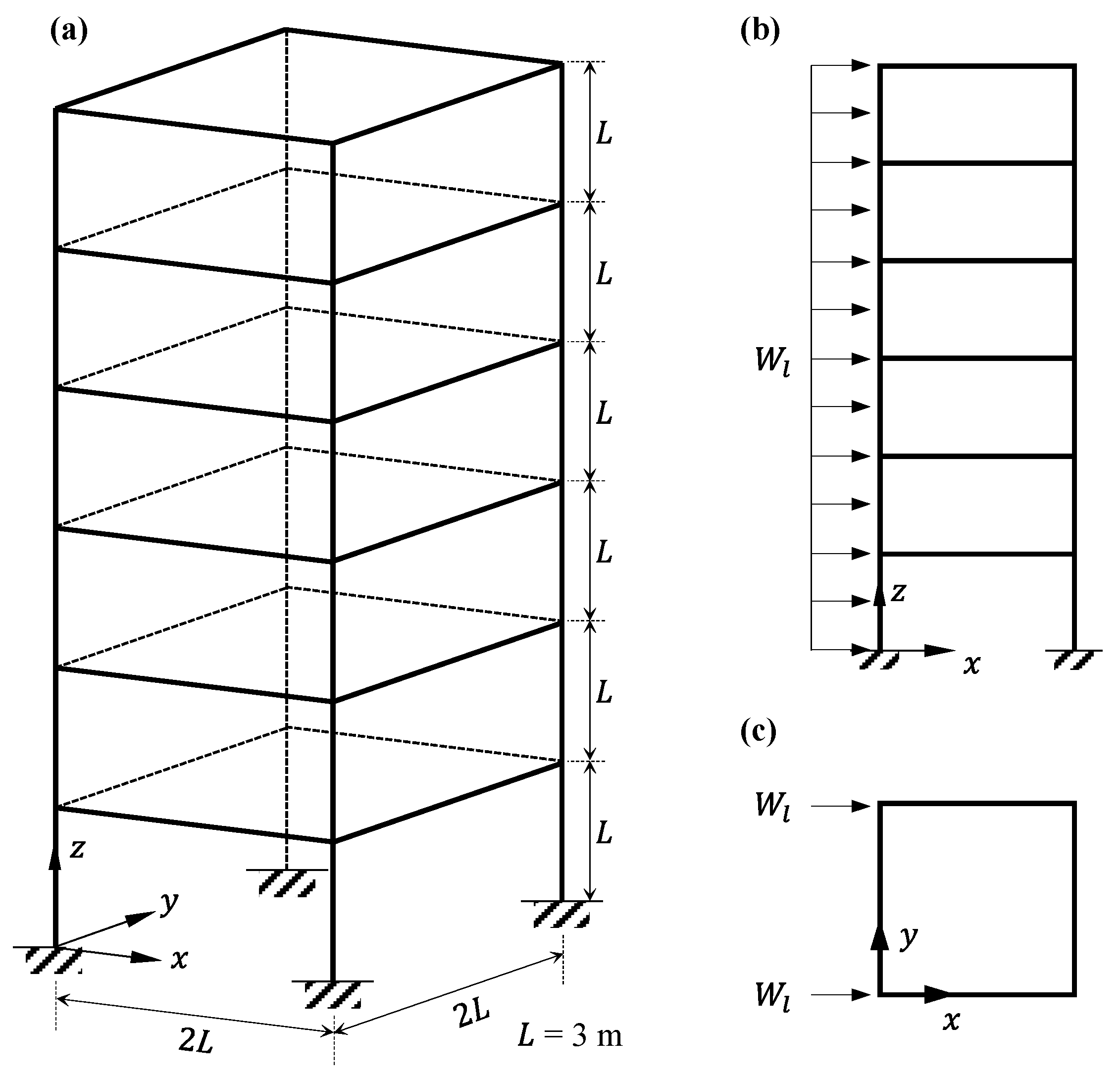
In the second FEM-based problem, a 3D space frame structure with 6-story is employed as shown in Figure 11. The configurations of input random variables are set the same as in the first FEM-based problem above. However, the load condition is modified to a live load acting in the horizontal direction, depicted as the lateral load ($W_l$) in Figure 11b,c. The mean of the live load is set to 75 N/m, and the CoV is set to 0.25 in accordance with the Eurocode and US standard [98,99].

Figure 11. Configuration of 6-story space frame. (a) 3D schematic view, (b) lateral load in x–z plane, and (c) lateral load in x–y plane.

The limit state function in Equation (24) can be modified considering the horizontal drift as follows:

$$g\left(\mathbf{X}\right)={\delta }_{h,\mathrm{l}\mathrm{i}\mathrm{m}\mathrm{i}\mathrm{t}}^{\prime }-FEM\left(\mathbf{X}\right)\left(\mathrm{m}\right)$$

(27)

where ${\delta }_{h,\mathrm{l}\mathrm{i}\mathrm{m}\mathrm{i}\mathrm{t}}^{\prime }=$ 0.01 (m) is the limit story drift according to Equation (22) and $FEM\left(\mathbf{X}\right)$ denotes the maximum story drift according to the results of FEM analysis. The meta model settings for this problem are set as follows: the number and width of hidden layers are set to 4 and 200, respectively. $n_0$, $n_1$ and $n_2$ are set to 100, 10 and 2, respectively; and $n_{\mathrm{c}\mathrm{r}}$ is set to $2n_0$, considering the complexity of the target system. The size of MCS population is set to 1 $\times$ 10⁵ considering the expected $P_f$.

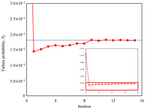
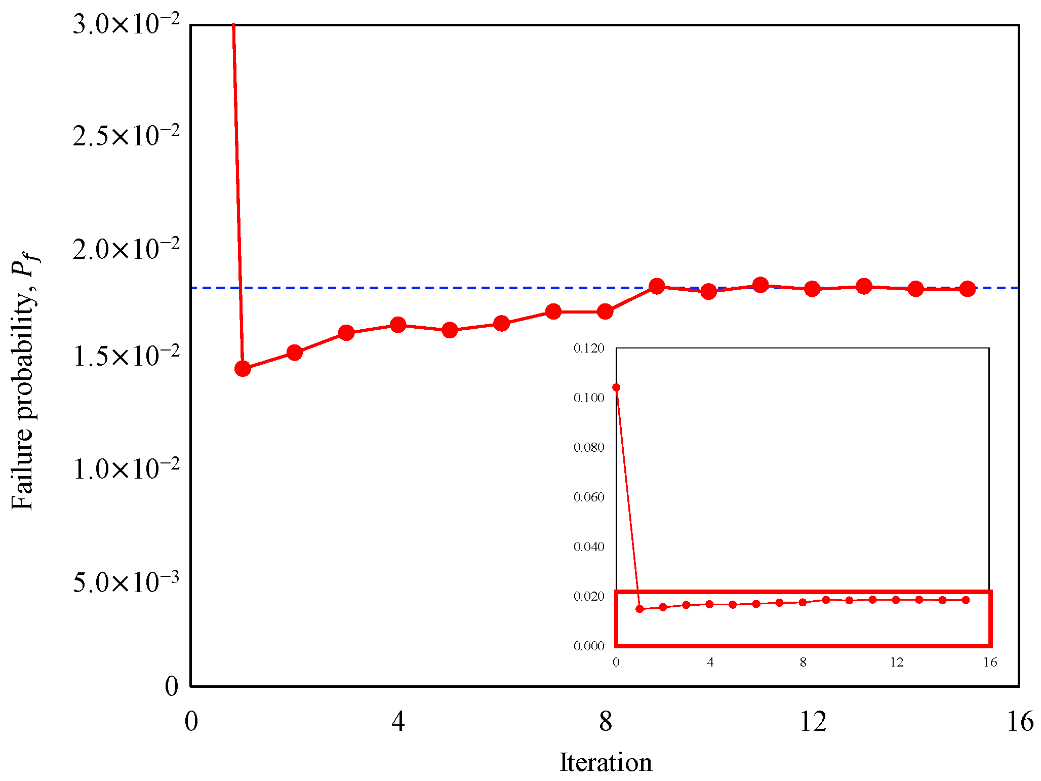
Table 11 shows the reliability analysis results for the 6-story space frame. The proposed ALDNN meta model calculated the $P_f$ as 1.800 × 10⁻², which was in great agreement with the solution by MCS. However, the $N_{\mathrm{c}\mathrm{a}\mathrm{l}\mathrm{l}}$ of the proposed method was only 208, while that of MCS was 1 × 10⁵. Consequently, the solution time in the proposed method was shorter than that of the MCS. Figure 12 shows the convergence history of the $P_f$.

Table 11. Results of reliability analysis for the 6-story space frame.

Method	Number of g Calls, Ncall	Failure Probability, Pf	Reliability Index, β	Relative Error of β, εβ (%)	Solution Time (s)
MCS	$1 \times$ 105	$1.829 \times$ 10−2	2.090	-	5423.775
ALDNN meta model	208	$1.800 \times$ 10−2	2.096	0.287	488.839

Figure 12. Failure probability convergence according to iteration in the 6-story space frame problem. The blue dotted line represents the converged failure probability.

3.2.3. Multi-Bay and Multi-Story Space Frame with Lateral Load

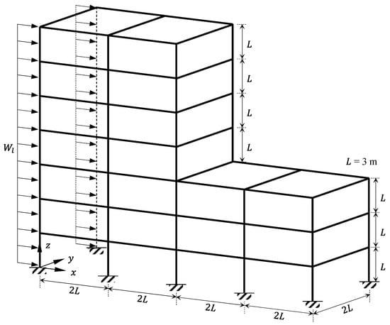
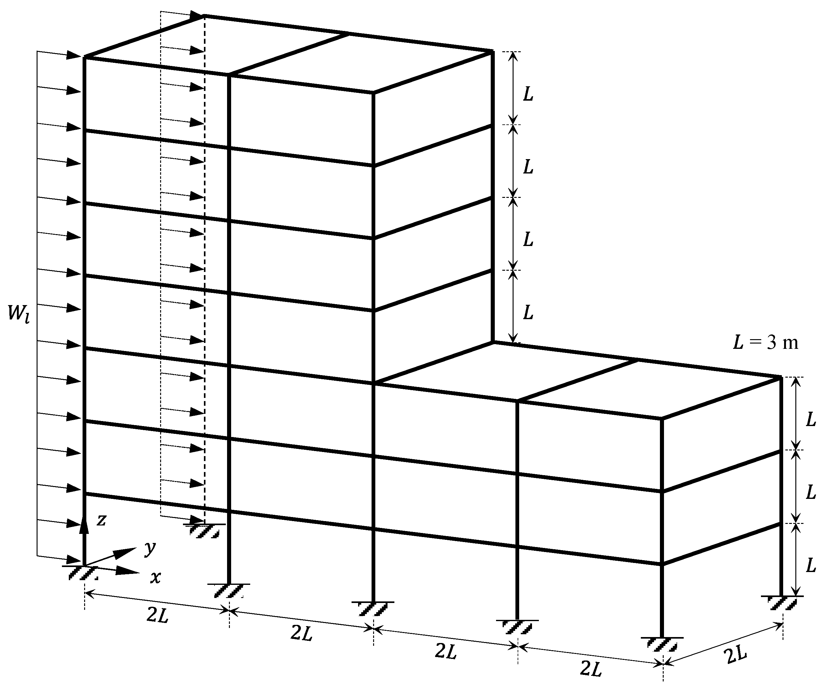
In the last FEM-based problem, a multi-bay and multi-story 3D space frame is employed (Figure 13). The configurations of input random variables are set the same as in the previous FEM-based problems. In this case, the lateral load setting is modified considering the overall strength of the structure. The mean of the lateral load is set to 180 N/m, and the CoV is set to 0.25 in accordance with the Eurocode and US standard [98,99].

Figure 13. Configuration of multi-bay and multi-story space frame with lateral load.

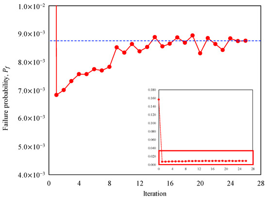
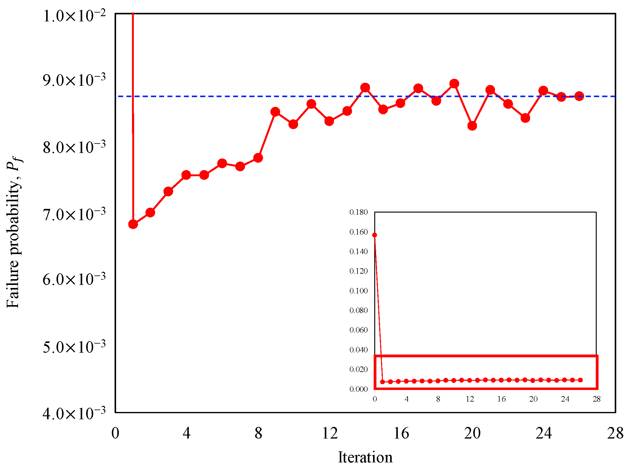
The limit state function and the ALDNN meta model configuration are set the same as in the second FEM-based problem. As a result, the proposed method estimated the $P_f$ as 8.750 $\times$ 10⁻³, while the corresponding MCS result was 8.760 × 10⁻³ (Table 12). The $N_{\mathrm{c}\mathrm{a}\mathrm{l}\mathrm{l}}$ of the proposed method was 230, whereas that of the MCS was significantly larger. It is noteworthy that the difference in solution time between the two methods became more pronounced compared to the second problem. The $P_f$ convergence of this problem is depicted in Figure 14.

Table 12. Results of reliability analysis for the multi-bay and multi-story space frame.

Method	Number of g Calls, Ncall	Failure Probability, Pf	Reliability Index, β	Relative Error of β, εβ (%)	Solution Time (s)
MCS	$1 \times$ 105	$1.829 \times$ 10−2	2.090	-	5423.775
ALDNN meta model	208	$1.800 \times$ 10−2	2.096	0.287	488.839

Figure 14. Failure probability convergence according to iteration in the multi-bay and multi-story space frame problem. The blue dotted line represents the converged failure probability.

4. Discussion

4.1. Benchmark-Based Performance and Comparative Insights

The benchmark studies demonstrated that the proposed ALDNN meta model achieves a favorable balance between accuracy and efficiency across a wide range of reliability problems. In all benchmark cases, the estimated failure probabilities and reliability indices were in close agreement with those obtained using MCS, while the number of limit state function calls was significantly reduced. This indicates that the proposed approach effectively addresses the classical trade-off between estimation accuracy and computational cost.

For the series system with four branches, which involves multiple failure modes and non-smooth limit state surfaces, the ALDNN meta model showed stable performance for both values of the parameter $k$ (Table 1 and Table 2). In contrast, some sampling-based methods, such as directional sampling, exhibited sensitivity to the geometric characteristics of the limit state surface, leading to notable accuracy degradation in the radially shaped case (Table 2). The proposed method maintained consistent accuracy with substantially fewer model evaluations, highlighting its robustness against changes in failure surface topology.

In the nonlinear oscillator problem, the ALDNN meta model achieved near-zero relative error in the reliability index with only a small number of limit state evaluations (Table 4). This result suggests that the proposed active learning strategy is particularly effective in capturing nonlinear response behavior when the failure probability is not extremely small. For the high-dimensional problem, the proposed method converged rapidly, often during the early stages of the active learning process (Table 5). This behavior can be attributed to the combined effect of weighted sampling and the relatively simple structure of the limit state function, which allowed the meta model to identify the failure boundary efficiently even in high-dimensional spaces. The 100-dimensional benchmark does not represent a strict upper limit of the proposed framework; extension to higher-dimensional topology optimization problems is feasible.

For the speed reducer shaft problem (Table 8), which involves heterogeneous probability distributions and rare failure events, the limitations of traditional analytical approximations such as FORM, SORM, and FOSPA became evident. While some surrogate-based methods required fewer model evaluations, their accuracy was insufficient. In contrast, the proposed ALDNN meta model achieved accurate estimates of both failure probability and reliability index with a small number of limit state evaluations, outperforming existing methods in terms of the overall accuracy–efficiency trade-off (Table 8).

Overall, the benchmark comparisons confirm that the proposed method achieves competitive or superior performance compared to existing reliability analysis techniques. It should be noted that MCS itself is subject to statistical variability due to random sampling. Therefore, minor discrepancies between MCS results and surrogate-based estimates should be interpreted within this inherent uncertainty. In this context, the total estimation error of the failure probability can be understood as the combination of surrogate classification error and finite Monte Carlo sampling error. To further quantify the estimation error more rigorously, future research should distinguish these two error components explicitly. One possible approach is to evaluate the true limit state function on a sufficiently large reference dataset and compare surrogate-based classifications with the true classifications to independently assess misclassification error. Further investigation into strategies for separately characterizing and controlling these error sources would enhance the statistical robustness of active-learning-based reliability methods.

4.2. Mechanistic Interpretation of the Three-Phase Active Learning Strategy

The effectiveness of the proposed ALDNN meta model can be understood by examining the role of each phase in the active learning framework. In Phase 1, the initial weighted sampling ensures that the training data are representative of the underlying probability distribution of the input variables (Figure 2). Accordingly, the initial convergence of the failure probability estimation was significantly improved. Although the initial predictions of failure probability are often unstable due to the limited number of training samples, the rescaling procedure mitigates numerical instability by normalizing the response magnitude. By constraining the scale of the surrogate output, excessive gradient magnitudes and oscillatory updates are reduced, leading to improved optimization conditioning and more stable convergence (Figure 4, Figure 6 and Figure 7).

Phase 2 focuses on identifying candidate samples located near the estimated limit state surface (Figure 2). By introducing adaptive thresholds on the predicted response values, the algorithm progressively narrows the candidate population toward regions that are most informative for reliability estimation. The decreasing threshold factor promotes a transition from global exploration to local exploitation, enabling the meta model to concentrate computational resources on the vicinity of the failure boundary.

In Phase 3, the algorithm further refines the surrogate model by removing training samples that are distant from the limit state surface (Figure 2). Such samples contribute limited information for boundary learning and may act as noise during training. The gradual tightening of the training thresholds, together with the reduction in the number of newly added samples after a predefined criterion is reached, enhances the precision of the failure boundary representation. As observed in the convergence histories (Figure 10, Figure 12 and Figure 14), this three-phase strategy explains the typical behavior in which early iterations exhibit oscillatory estimates of failure probability, followed by stable and monotonic convergence as the active learning process progresses. In addition, weighted sampling was applied not only in Phase 1 but also in Phases 2 and 3, thereby enabling more efficient and accurate prediction of the failure probability in the later stages of the algorithm.

To clarify the robustness of the candidate filtering mechanism, the possibility of false-negative pruning is briefly discussed. The filtering is performed based on the surrogate prediction rather than the true limit state function. Therefore, a true failure sample can be excluded only when the surrogate approximation error is sufficiently large relative to the threshold width. In early iterations, the candidate window is intentionally kept wide to preserve global exploration and reduce the risk of premature exclusion. As training progresses, the surrogate error becomes increasingly concentrated, further lowering this risk. Thus, the filtering mechanism controls the exploration–exploitation trade-off without arbitrarily eliminating the failure domain.

4.3. Computational Cost and Scalability

The computational efficiency of the proposed method depends on the relative cost of limit state evaluations and surrogate training. Although the MCS population is pre-generated, only the input samples are stored, and the dominant computational burden arises from evaluating the true limit state function rather than from memory usage. For problems with explicitly defined and inexpensive limit state functions, the training overhead of the deep neural network may outweigh the benefits of reducing the number of model evaluations. However, for problems with implicitly defined limit states, particularly FEM-based structural systems, the substantial reduction in limit state evaluations leads to significant savings in computational time.

The time efficiency of ALDNN depends on the relative cost of evaluating the true limit state function and training the surrogate model. When the evaluation cost of $g\left(X\right)$ is sufficiently high, the reduction in the number of true function calls outweighs the training overhead; however, for inexpensive analytical functions, direct MCS may remain more time-efficient.

The FEM-based problems varied in complexity, with an increase in the number of degrees of freedom (DoFs) for each FEM analysis. The number of DoFs for FEM in the 2-bay, 6-story, and multi-bay with multi-story frame examples were 78, 744, and 1914, respectively. When comparing the computational cost with the increasing number of DoFs, the solution time of MCS increased linearly. However, the proposed meta model method exhibited scalability, meaning that the required computational cost did not increase substantially even as the complexity of the target system increased (Table 10, Table 11 and Table 12). This scalability arises from the active learning strategy, which concentrates evaluations near the failure boundary rather than uniformly sampling the entire input space (Figure 3).

4.4. Practical Implications, Limitations, and Future Work

From a practical engineering perspective, the proposed ALDNN meta model enables efficient reliability analysis in scenarios where direct MCS is infeasible due to excessive computational cost. The method is particularly well suited for applications such as design optimization, comparative evaluation of structural alternatives, and reliability-based maintenance planning.

For practical implementation, the selection of initial and incremental sample sizes should be adjusted according to the complexity of the target system. Larger initial sample sizes may be required for highly nonlinear or high-dimensional problems, while smaller incremental updates are sufficient during later refinement stages. The convergence criterion for the relative error of failure probability provides a flexible mechanism for balancing accuracy and computational cost, allowing users to tailor the analysis to specific engineering requirements.

Nevertheless, the present study focused on serviceability limit states, which may not fully represent ultimate structural safety. Future work should extend the proposed framework to ultimate limit states and damage-based performance criteria. Furthermore, although practical guidelines for hyperparameter selection were discussed, a more systematic and theoretically grounded optimization of parameters such as $n_0$, $n_1$, $n_2$ remains an open challenge, similar to many deep learning and optimization-based methods. Moreover, future work should explore adaptive strategies for dynamically adjusting the candidate window based on surrogate uncertainty rather than fixed attenuation factors. Further research is therefore required to enhance hyperparameter robustness, address extremely rare failure events, and integrate uncertainty-aware or multi-fidelity learning strategies.

5. Conclusions

This study presented the development of an ALDNN meta model algorithm that improves the efficiency and accuracy of reliability analysis. The proposed algorithm was composed of three major phases: Phase 1 conducted the initial sampling and rescaling. Phase 2 conducted the filtering of the candidate population; and phase 3 performed the removing noise and precise prediction. To demonstrate the performance of the proposed meta model, the benchmark problems and the FEM-based problems were employed.

The benchmark problems included four different limit states with distinct features, such as multiple failure modes, nonlinearity, high-dimensionality, and various types of distribution. In these benchmark cases, the proposed method demonstrated competitive or improved performance in terms of accuracy and reduction in limit state function evaluations compared to conventional simulation approaches. Although the proposed method initially exhibited unstable estimates of $P_f$, the predictions gradually stabilized as the multi-phase active learning strategy was implemented. In the FEM-based problems, where the limit states were implicitly defined, the applicability of the proposed meta model was verified. Three different frame structures were employed to conduct structural reliability analysis, and the results of $P_f$ and $\beta$ were in excellent agreement with those obtained using MCS. In terms of computation time, the proposed meta model showed efficiency advantages in problems where the limit state function evaluation is computationally demanding.

It should be noted that the FEM-based structural reliability analysis in this study considered serviceability limit states defined by displacement criteria within a linear analysis framework. Such assumptions do not fully represent ultimate structural safety. Therefore, future research should extend the proposed framework to ultimate limit states and nonlinear structural behavior to further assess its applicability to safety-critical design scenarios.

References

- Ang, A.H.; Tang, W.H. Probability Concepts in Engineering Planning and Design; John Wiley & Sons: New York, NY, USA, 1975; Volume 1. [Google Scholar]
- Haldar, A.; Mahadevan, S. Reliability Assessment Using Stochastic Finite Element Analysis; John Wiley & Sons: New York, NY, USA, 2000. [Google Scholar]
- Rackwitz, R. Reliability analysis—A review and some perspectives. Struct. Saf. 2001, 23, 365–395. [Google Scholar] [CrossRef] [Scilit]
- Melchers, R.E.; Beck, A.T. Structural Reliability Analysis and Prediction; John Wiley & Sons: Hoboken, NJ, USA, 2018. [Google Scholar]
- Zhou, T.; Peng, Y.; Li, J. An efficient reliability method combining adaptive global metamodel and probability density evolution method. Mech. Syst. Signal Process. 2019, 131, 592–616. [Google Scholar] [CrossRef] [Scilit]
- Hasofer, A.M.; Lind, N.C. Exact and invariant second-moment code format. J. Eng. Mech. Div. 1974, 100, 111–121. [Google Scholar] [CrossRef] [Scilit]
- Rackwitz, R.; Flessler, B. Structural reliability under combined random load sequences. Comput. Struct. 1978, 9, 489–494. [Google Scholar] [CrossRef] [Scilit]
- Breitung, K. Asymptotic approximations for multinormal integrals. J. Eng. Mech. 1984, 110, 357–366. [Google Scholar] [CrossRef] [Scilit]
- Der Kiureghian, A.; Lin, H.-Z.; Hwang, S.-J. Second-order reliability approximations. J. Eng. Mech. 1987, 113, 1208–1225. [Google Scholar] [CrossRef] [Scilit]
- Mitteau, J.-C. Error evaluations for the computation of failure probability in static structural reliability problems. Probabilistic Eng. Mech. 1999, 14, 119–136. [Google Scholar] [CrossRef] [Scilit]
- Du, X.; Sudjianto, A. First order saddlepoint approximation for reliability analysis. AIAA J. 2004, 42, 1199–1207. [Google Scholar] [CrossRef] [Scilit]
- Metropolis, N.; Ulam, S. The monte carlo method. J. Am. Stat. Assoc. 1949, 44, 335–341. [Google Scholar] [CrossRef] [PubMed]
- Kahn, H. Use of Different Monte Carlo Sampling Techniques; Rand Corporation: Santa Monica, CA, USA, 1955. [Google Scholar]
- Glasserman, P.; Heidelberger, P.; Shahabuddin, P. Variance reduction techniques for estimating value-at-risk. Manag. Sci. 2000, 46, 1349–1364. [Google Scholar] [CrossRef] [Scilit]
- Grabaskas, D.; Nakayama, M.K.; Denning, R.; Aldemir, T. Advantages of variance reduction techniques in establishing confidence intervals for quantiles. Reliab. Eng. Syst. Saf. 2016, 149, 187–203. [Google Scholar] [CrossRef] [Scilit]
- Hohenbichler, M.; Rackwitz, R. Improvement of second-order reliability estimates by importance sampling. J. Eng. Mech. 1988, 114, 2195–2199. [Google Scholar] [CrossRef] [Scilit]
- Ang, G.L.; Ang, A.H.; Tang, W.H. Optimal importance-sampling density estimator. J. Eng. Mech. 1992, 118, 1146–1163. [Google Scholar] [CrossRef] [Scilit]
- Tokdar, S.T.; Kass, R.E. Importance sampling: A review. Wiley Interdiscip. Rev. Comput. Stat. 2010, 2, 54–60. [Google Scholar] [CrossRef] [Scilit]
- McKay, M.D.; Beckman, R.J.; Conover, W.J. A comparison of three methods for selecting values of input variables in the analysis of output from a computer code. Technometrics 1979, 42, 55–61. [Google Scholar] [CrossRef]
- Helton, J.C.; Davis, F.J. Latin hypercube sampling and the propagation of uncertainty in analyses of complex systems. Reliab. Eng. Syst. Saf. 2003, 81, 23–69. [Google Scholar] [CrossRef] [Scilit]
- Bucher, C.G. Adaptive sampling—An iterative fast Monte Carlo procedure. Struct. Saf. 1988, 5, 119–126. [Google Scholar] [CrossRef] [Scilit]
- Au, S.-K.; Beck, J.L. Estimation of small failure probabilities in high dimensions by subset simulation. Probabilistic Eng. Mech. 2001, 16, 263–277. [Google Scholar] [CrossRef] [Scilit]
- Papadopoulos, V.; Giovanis, D.G.; Lagaros, N.D.; Papadrakakis, M. Accelerated subset simulation with neural networks for reliability analysis. Comput. Methods Appl. Mech. Eng. 2012, 223, 70–80. [Google Scholar] [CrossRef] [Scilit]
- Bjerager, P. Probability integration by directional simulation. J. Eng. Mech. 1988, 114, 1285–1302. [Google Scholar] [CrossRef] [Scilit]
- Nie, J.; Ellingwood, B.R. Directional methods for structural reliability analysis. Struct. Saf. 2000, 22, 233–249. [Google Scholar] [CrossRef] [Scilit]
- Pradlwarter, H.; Schueller, G.I.; Koutsourelakis, P.-S.; Charmpis, D.C. Application of line sampling simulation method to reliability benchmark problems. Struct. Saf. 2007, 29, 208–221. [Google Scholar] [CrossRef] [Scilit]
- Lu, Z.; Song, S.; Yue, Z.; Wang, J. Reliability sensitivity method by line sampling. Struct. Saf. 2008, 30, 517–532. [Google Scholar] [CrossRef] [Scilit]
- Song, J.; Wei, P.; Valdebenito, M.; Beer, M. Active learning line sampling for rare event analysis. Mech. Syst. Signal Process. 2021, 147, 107113. [Google Scholar] [CrossRef] [Scilit]
- Cavazzuti, M. Optimization Methods: From Theory to Design Scientific and Technological Aspects in Mechanics; Springer Science & Business Media: Modena, Italy, 2012. [Google Scholar]
- Dubourg, V.; Sudret, B.; Deheeger, F. Metamodel-based importance sampling for structural reliability analysis. Probabilistic Eng. Mech. 2013, 33, 47–57. [Google Scholar] [CrossRef] [Scilit]
- Bichon, B.J.; McFarland, J.M.; Mahadevan, S. Efficient surrogate models for reliability analysis of systems with multiple failure modes. Reliab. Eng. Syst. Saf. 2011, 96, 1386–1395. [Google Scholar] [CrossRef] [Scilit]
- Teixeira, R.; Nogal, M.; O’Connor, A. Adaptive approaches in metamodel-based reliability analysis: A review. Struct. Saf. 2021, 89, 102019. [Google Scholar] [CrossRef] [Scilit]
- Li, W.; Geng, R.; Chen, S. CSP-free adaptive Kriging surrogate model method for reliability analysis with small failure probability. Reliab. Eng. Syst. Saf. 2024, 243, 109898. [Google Scholar] [CrossRef] [Scilit]
- Marrel, A.; Iooss, B.; Laurent, B.; Roustant, O. Calculations of Sobol indices for the Gaussian process metamodel. Reliab. Eng. Syst. Saf. 2009, 94, 742–751. [Google Scholar] [CrossRef] [Scilit]
- Ge, Q.; Ciuffo, B.; Menendez, M. Combining screening and metamodel-based methods: An efficient sequential approach for the sensitivity analysis of model outputs. Reliab. Eng. Syst. Saf. 2015, 134, 334–344. [Google Scholar] [CrossRef] [Scilit]
- Faravelli, L. Response-surface approach for reliability analysis. J. Eng. Mech. 1989, 115, 2763–2781. [Google Scholar] [CrossRef] [Scilit]
- Bucher, C.G.; Bourgund, U. A fast and efficient response surface approach for structural reliability problems. Struct. Saf. 1990, 7, 57–66. [Google Scholar] [CrossRef] [Scilit]
- Romero, V.; Swiler, L.; Giunta, A. Construction of response surfaces based on progressive-lattice-sampling experimental designs with application to uncertainty propagation. Struct. Saf. 2004, 26, 201–219. [Google Scholar] [CrossRef] [Scilit]
- Kaymaz, I. Application of kriging method to structural reliability problems. Struct. Saf. 2005, 27, 133–151. [Google Scholar] [CrossRef] [Scilit]
- Cressie, N. Statistics for Spatial Data; John Wiley & Sons: Hoboken, NJ, USA, 2015. [Google Scholar]
- Zhang, X.; Lu, Z.; Cheng, K. Reliability index function approximation based on adaptive double-loop Kriging for reliability-based design optimization. Reliab. Eng. Syst. Saf. 2021, 216, 108020. [Google Scholar] [CrossRef] [Scilit]
- Shi, Y.; Lin, C.; Ma, Y.; Shen, J. Active Learning Kriging-based Multi-objective Modeling and Optimization for System Reliability-based Robust Design. Reliab. Eng. Syst. Saf. 2024, 245, 110007. [Google Scholar] [CrossRef] [Scilit]
- Schueremans, L.; Van Gemert, D. Benefit of splines and neural networks in simulation based structural reliability analysis. Struct. Saf. 2005, 27, 246–261. [Google Scholar] [CrossRef] [Scilit]
- Cheraghi, N.; Miri, M.; Rashki, M. An adaptive artificial neural network for reliability analyses of complex engineering systems. Appl. Soft Comput. 2023, 132, 109866. [Google Scholar] [CrossRef] [Scilit]
- Zhang, W.; Gu, X.; Hong, L.; Han, L.; Wang, L. Comprehensive review of machine learning in geotechnical reliability analysis: Algorithms, applications and further challenges. Appl. Soft Comput. 2023, 136, 110066. [Google Scholar] [CrossRef] [Scilit]
- Liu, D.; Duan, X.; Wang, S.; Cui, X.; Wu, X.; Niu, Y.; Shi, J. A reliability estimation method based on signal feature extraction and artificial neural network supported Wiener process with random effects. Appl. Soft Comput. 2023, 136, 110044. [Google Scholar] [CrossRef] [Scilit]
- Papadrakakis, M.; Papadopoulos, V.; Lagaros, N.D. Structural reliability analyis of elastic-plastic structures using neural networks and Monte Carlo simulation. Comput. Methods Appl. Mech. Eng. 1996, 136, 145–163. [Google Scholar] [CrossRef] [Scilit]
- Cardoso, J.B.; de Almeida, J.R.; Dias, J.M.; Coelho, P.G. Structural reliability analysis using Monte Carlo simulation and neural networks. Adv. Eng. Softw. 2008, 39, 505–513. [Google Scholar] [CrossRef] [Scilit]
- Chojaczyk, A.A.; Teixeira, A.P.; Neves, L.C.; Cardoso, J.B.; Soares, C.G. Review and application of Artificial Neural Networks models in reliability analysis of steel structures. Struct. Saf. 2015, 52, 78–89. [Google Scholar] [CrossRef] [Scilit]
- Rocco, C.M.; Moreno, J.A. Fast Monte Carlo reliability evaluation using support vector machine. Reliab. Eng. Syst. Saf. 2002, 76, 237–243. [Google Scholar] [CrossRef] [Scilit]
- Song, H.; Choi, K.K.; Lee, I.; Zhao, L.; Lamb, D. Adaptive virtual support vector machine for reliability analysis of high-dimensional problems. Struct. Multidiscip. Optim. 2013, 47, 479–491. [Google Scholar] [CrossRef] [Scilit]
- Bucher, C.; Most, T. A comparison of approximate response functions in structural reliability analysis. Probabilistic Eng. Mech. 2008, 23, 154–163. [Google Scholar] [CrossRef] [Scilit]
- LeCun, Y.; Bengio, Y.; Hinton, G. Deep learning. Nature 2015, 521, 436–444. [Google Scholar] [CrossRef] [Scilit]
- Schmidhuber, J. Deep learning in neural networks: An overview. Neural Netw. 2015, 61, 85–117. [Google Scholar] [CrossRef] [Scilit] [PubMed]
- Silver, D.; Huang, A.; Maddison, C.J.; Guez, A.; Sifre, L.; Van Den Driessche, G.; Schrittwieser, J.; Antonoglou, I.; Panneershelvam, V.; Lanctot, M. Mastering the game of Go with deep neural networks and tree search. Nature 2016, 529, 484–489. [Google Scholar] [CrossRef] [Scilit]
- Afshari, S.S.; Enayatollahi, F.; Xu, X.; Liang, X. Machine learning-based methods in structural reliability analysis: A review. Reliab. Eng. Syst. Saf. 2022, 219, 108223. [Google Scholar] [CrossRef] [Scilit]
- Kim, T.; Song, J.; Kwon, O.-S. Probabilistic evaluation of seismic responses using deep learning method. Struct. Saf. 2020, 84, 101913. [Google Scholar] [CrossRef] [Scilit]
- Xie, H.; Tang, L.; Zhu, H.; Cheng, X.; Bie, Z. Robustness assessment and enhancement of deep reinforcement learning-enabled load restoration for distribution systems. Reliab. Eng. Syst. Saf. 2023, 237, 109340. [Google Scholar] [CrossRef] [Scilit]
- Li, J.; Long, X.; Deng, X.; Jiang, W.; Zhou, K.; Jiang, C.; Zhang, X. A principled distance-aware uncertainty quantification approach for enhancing the reliability of physics-informed neural network. Reliab. Eng. Syst. Saf. 2024, 245, 109963. [Google Scholar] [CrossRef] [Scilit]
- Zhou, T.; Droguett, E.L.; Mosleh, A. Physics-informed deep learning: A promising technique for system reliability assessment. Appl. Soft Comput. 2022, 126, 109217. [Google Scholar] [CrossRef] [Scilit]
- Liu, J.; Liu, L.; Li, S.; Tang, Z.; Wang, C. Study of structural reliability evaluation method based on deep BP neural network. In Proceedings of the 2018 Prognostics and System Health Management Conference (PHM-Chongqing), Chongqing, China, 26–28 October 2018; pp. 500–505. [Google Scholar]
- Li, M.; Wang, Z. Deep learning for high-dimensional reliability analysis. Mech. Syst. Signal Process. 2020, 139, 106399. [Google Scholar] [CrossRef] [Scilit]
- Xiang, Z.; Bao, Y.; Tang, Z.; Li, H. Deep reinforcement learning-based sampling method for structural reliability assessment. Reliab. Eng. Syst. Saf. 2020, 199, 106901. [Google Scholar] [CrossRef] [Scilit]
- Sutton, R.S.; Barto, A.G. Reinforcement Learning: An Introduction; MIT Press: Mountain View, CA, USA, 2018. [Google Scholar]
- Tvedt, L. Distribution of quadratic forms in normal space—Application to structural reliability. J. Eng. Mech. 1990, 116, 1183–1197. [Google Scholar] [CrossRef] [Scilit]
- Echard, B.; Gayton, N.; Lemaire, M. AK-MCS: An active learning reliability method combining Kriging and Monte Carlo simulation. Struct. Saf. 2011, 33, 145–154. [Google Scholar] [CrossRef] [Scilit]
- Xiang, Z.; Chen, J.; Bao, Y.; Li, H. An active learning method combining deep neural network and weighted sampling for structural reliability analysis. Mech. Syst. Signal Process. 2020, 140, 106684. [Google Scholar] [CrossRef] [Scilit]
- Bao, Y.; Xiang, Z.; Li, H. Adaptive subset searching-based deep neural network method for structural reliability analysis. Reliab. Eng. Syst. Saf. 2021, 213, 107778. [Google Scholar] [CrossRef] [Scilit]
- Lieu, Q.X.; Nguyen, K.T.; Dang, K.D.; Lee, S.; Kang, J.; Lee, J. An adaptive surrogate model to structural reliability analysis using deep neural network. Expert Syst. Appl. 2022, 189, 116104. [Google Scholar] [CrossRef] [Scilit]
- Duchi, J.; Hazan, E.; Singer, Y. Adaptive subgradient methods for online learning and stochastic optimization. J. Mach. Learn. Res. 2011, 12, 2121–2159. [Google Scholar]
- Tieleman, T.; Hinton, G. Lecture 6.5-rmsprop: Divide the gradient by a running average of its recent magnitude. Coursera Neural Netw. Mach. Learn. 2012, 4, 26–31. [Google Scholar]
- Kingma, D.P.; Ba, J. Adam: A method for stochastic optimization. arXiv 2014, arXiv:1412.6980. [Google Scholar] [CrossRef] [Scilit]
- Maas, A.L.; Hannun, A.Y.; Ng, A.Y. Rectifier nonlinearities improve neural network acoustic models. In Proceedings of the 30th International Conference on Machine Learning, Atlanta, GA, USA, 17–19 June 2013; p. 3. [Google Scholar]
- Li, M.; Zhang, T.; Chen, Y.; Smola, A.J. Efficient mini-batch training for stochastic optimization. In Proceedings of the 20th ACM SIGKDD International Conference on Knowledge Discovery and Data Mining, New York, NY, USA, 24–27 August 2014; pp. 661–670. [Google Scholar]
- Prechelt, L. Automatic early stopping using cross validation: Quantifying the criteria. Neural Netw. 1998, 11, 761–767. [Google Scholar] [CrossRef] [Scilit]
- Yao, Y.; Rosasco, L.; Caponnetto, A. On early stopping in gradient descent learning. Constr. Approx. 2007, 26, 289–315. [Google Scholar] [CrossRef] [Scilit]
- Goodfellow, I.; Bengio, Y.; Courville, A. Deep Learning; MIT Press: Cambridge, MA, USA, 2016. [Google Scholar]
- Braverman, V.; Ostrovsky, R.; Vorsanger, G. Weighted sampling without replacement from data streams. Inf. Process. Lett. 2015, 115, 923–926. [Google Scholar] [CrossRef] [Scilit]
- Efraimidis, P.S.; Spirakis, P.G. Weighted random sampling with a reservoir. Inf. Process. Lett. 2006, 97, 181–185. [Google Scholar] [CrossRef] [Scilit]
- Sun, Z.; Wang, J.; Li, R.; Tong, C. LIF: A new Kriging based learning function and its application to structural reliability analysis. Reliab. Eng. Syst. Saf. 2017, 157, 152–165. [Google Scholar] [CrossRef] [Scilit]
- Li, X.; Gong, C.; Gu, L.; Gao, W.; Jing, Z.; Su, H. A sequential surrogate method for reliability analysis based on radial basis function. Struct. Saf. 2018, 73, 42–53. [Google Scholar] [CrossRef] [Scilit]
- Marelli, S.; Sudret, B. An active-learning algorithm that combines sparse polynomial chaos expansions and bootstrap for structural reliability analysis. Struct. Saf. 2018, 75, 67–74. [Google Scholar] [CrossRef] [Scilit]
- Vahedi, J.; Ghasemi, M.R.; Miri, M. An adaptive divergence-based method for structural reliability analysis via multiple Kriging models. Appl. Math. Model. 2018, 62, 542–561. [Google Scholar] [CrossRef] [Scilit]
- Schueremans, L.; Van Gemert, D. Use of Kriging as meta-model in simulation procedures for structural reliability. In Proceedings of the International Conference on Structural Safety and Reliability, Rome, Italy, 19–23 June 2005; pp. 2483–2490. [Google Scholar]
- Rajashekhar, M.R.; Ellingwood, B.R. A new look at the response surface approach for reliability analysis. Struct. Saf. 1993, 12, 205–220. [Google Scholar] [CrossRef] [Scilit]
- Korean Society of Steel Construction. KSSC-21-02 Steel Structure Design; Gumi Publishing: Seoul, Republic of Korea, 2021. [Google Scholar]
- Bartlett, F.; Hong, H.P.; Zhou, W. Load factor calibration for the proposed 2005 edition of the National Building Code of Canada: Companion-action load combinations. Can. J. Civ. Eng. 2003, 30, 440–448. [Google Scholar] [CrossRef] [Scilit]
- Afshan, S.; Francis, P.; Baddoo, N.; Gardner, L. Reliability analysis of structural stainless steel design provisions. J. Constr. Steel Res. 2015, 114, 293–304. [Google Scholar] [CrossRef] [Scilit]
- Arrayago, I.; Rasmussen, K.J.; Real, E. Statistical analysis of the material, geometrical and imperfection characteristics of structural stainless steels and members. J. Constr. Steel Res. 2020, 175, 106378. [Google Scholar] [CrossRef] [Scilit]
- Piliounis, G.; Lagaros, N.D. Reliability analysis of geostructures based on metaheuristic optimization. Appl. Soft Comput. 2014, 22, 544–565. [Google Scholar] [CrossRef] [Scilit]
- Leffler, B. A statistical study of the mechanical properties of hot rolled stainless plate. In Proceedings of the Nordic Symposium on Mechanical Properties of Stainless Steels, Sigtuna, Sweden, 16–17 October 1990; pp. 32–42. [Google Scholar]
- Gunn, R. Duplex Stainless Steels: Microstructure, Properties and Applications; Woodhead Publishing: Milton Keynes, UK, 1997. [Google Scholar]
- Huang, Y.; Young, B. Material properties of cold-formed lean duplex stainless steel sections. Thin-Walled Struct. 2012, 54, 72–81. [Google Scholar] [CrossRef] [Scilit]
- Afshan, S.; Gardner, L. Experimental study of cold-formed ferritic stainless steel hollow sections. J. Struct. Eng. 2013, 139, 717–728. [Google Scholar] [CrossRef] [Scilit]
- Theofanous, M.; Saliba, N.; Zhao, O.; Gardner, L. Ultimate response of stainless steel continuous beams. Thin-Walled Struct. 2014, 83, 115–127. [Google Scholar] [CrossRef] [Scilit]
- Arrayago, I.; Rasmussen, K.J. System-based reliability analysis of stainless steel frames under gravity loads. Eng. Struct. 2021, 231, 111775. [Google Scholar] [CrossRef] [Scilit]
- EN 10088-1:2014; Stainless Steels—Part 1: List of Stainless Steels. European Committee for Standardization: Brussels, Belgium, 2005.
- EN 1993-1-4:2006&A1:2015; Eurocode 3: Design of Steel Structures—Part 1–4: General Rules—Supplementary Rules for Stainless Steels. European Committee for Standardization: Brussels, Belgium, 2015.
- ASCE/SEI 7-10; Minimum Design Loads for Buildings and Other Structures. American Society of Civil Engineers: Reston, VA, USA, 2010. [CrossRef] [Scilit]
Disclaimer/Publisher’s Note: The statements, opinions and data contained in all publications are solely those of the individual author(s) and contributor(s) and not of MDPI and/or the editor(s). MDPI and/or the editor(s) disclaim responsibility for any injury to people or property resulting from any ideas, methods, instructions or products referred to in the content. |
© 2026 by the author. Licensee MDPI, Basel, Switzerland. This article is an open access article distributed under the terms and conditions of the Creative Commons Attribution (CC BY) license.