


Abstract
Microlevel loss reserving can use claim-level information that aggregate methods such as chain ladder cannot exploit. This paper predicts individual ultimate claim amounts with a hybrid neural network that combines a feedforward network for static claim characteristics with a long short-term memory network for the payment history of each claim. The framework is evaluated on a simulated motor-insurance portfolio of claims closed at the final valuation date, so that predictions can be compared with known ultimates; the estimation of RBNS and IBNR reserves is outside the scope of the study. Severity strata are formed by k-means clustering of the ultimate amount, and covariates are selected with the Boruta algorithm, both fitted to the training claims only. With complete payment histories, the hybrid models produce much smaller aggregate deviations than chain ladder for recent accident years, while chain ladder remains competitive for mature ones. Boruta retains one or two covariates; the reduced set helps only the untuned full-portfolio model, whereas in the tuned severity-stratum models the full covariate set lowers the test MAE by one third to one half. In a backtest with payment histories truncated at December 2019, the hybrid models keep an accident-year MAPE of 2.1–3.0%, against 16.5% for chain ladder, but improve on the amount paid to date by only 10–15% for claims still open at that date. The results indicate that feature selection, segmentation, and model tuning should be evaluated jointly.
Keywords:
chain ladder; feature selection; feedforward neural networks; LSTM; hybrid neural networks; individual-claim reserving; k-means clustering; loss reserving; risk modelling MSC:
62P05; 62M45; 68T07; 62-08
1. Introduction
Accurate estimation of outstanding claim liabilities is central to the financial stability of nonlife-insurance undertakings and to compliance with regulatory frameworks such as Solvency II. In particular, the valuation of reported but not settled (RBNS) and incurred but not reported (IBNR) claims remains a core actuarial task. Traditional reserving techniques, including the chain ladder, the Bornhuetter–Ferguson method [1], and frequency–severity approaches, rely on aggregated historical data and impose simplifying structural assumptions. While these methods remain widely used in practice, their aggregated nature limits their ability to capture heterogeneity, nonlinear effects, and time-dependent dynamics at the individual-claim level.
The increasing availability of granular claims data, together with advances in machine learning, has motivated a growing literature on microlevel reserving models. Early contributions explored neural-network-based extensions of classical reserving techniques. For instance, Harej et al. [2] applied cascades of multilayer perceptrons to simulated claim portfolios and found that they outperformed chain ladder when development patterns changed over time, but not when patterns were stable. Gabrielli and Wüthrich [3] introduced a stochastic simulation framework based on multiple neural networks to generate realistic claim-development paths, while Wüthrich [4] used regression trees to predict the development of individual claims from claim-level covariates. Although these approaches increase granularity, they either rely heavily on simulation, entail substantial computational complexity, or do not explicitly model temporal claim development.
Subsequent studies have further highlighted the limitations of aggregated reserving methods when applied to small or heterogeneous portfolios. Gabrielli and Wüthrich [5] backtested the chain-ladder method on simulated triangles for companies of different sizes, showing that it performs well on average but that, for smaller portfolios, the outcomes deviate much more from its reserves and Mack’s formula underestimates the prediction uncertainty, and Gabrielli et al. [6] embedded the overdispersed Poisson reserving model into a neural-network architecture, demonstrating that learned features can improve on the classical model. At the microlevel, Bücher and Rosenstock [7] proposed mixture models for individual reporting delays, with parameters linked to claim features through neural networks, and showed improved predictions of outstanding claim counts in nonhomogeneous portfolios. Other contributions have focused on sequential models: Somaratne [8] applied bidirectional LSTM architectures to forecast ultimate losses, and Feng and Li [9] generalised the sequence-to-sequence DeepTriangle framework, reporting gains over chain ladder and the original DeepTriangle. These approaches illustrate the potential of deep learning for reserving, but often require large datasets, strong modelling assumptions, or carefully calibrated prior inputs.
More recently, Chaoubi et al. [10] proposed a discrete-time LSTM framework for microlevel reserving that jointly classifies the occurrence of a payment and predicts its size, treating static claim characteristics as time-varying inputs, and that adjusts the reserve prediction for extreme payments through a generalised Pareto model. Their results, obtained on both simulated and real insurance portfolios, demonstrate that LSTM-based architectures can outperform traditional benchmarks in certain settings, particularly for large claims, while also highlighting the sensitivity of such models to data quality, portfolio heterogeneity, and model specification. Schneider and Schwab [11] extended this line of research by introducing a hybrid neural-network framework that explicitly separates static and dynamic features and combines classification and regression tasks for RBNS claims, demonstrating improved performance on proprietary industrial-insurance data.
Recent work has continued to widen the methodological toolkit. Avanzi et al. [12] showed that combining several reserving models in an ensemble improves distributional forecasts of outstanding claims relative to any single model. Richman and Wüthrich [13] reformulated the chain-ladder method in terms of projection-to-ultimate factors estimated from the latest observations, which provides a direct route from aggregate reserving to individual-claims models, and Avanzi et al. [14] cast microlevel reserving as a reinforcement-learning problem in which liability estimates are updated as claims develop, so that open as well as settled claims contribute to learning. These studies point towards ensembles of networks, explicit links with classical reserving, and the use of open claims, three directions that bear directly on the limitations of the present study set out in Section 4.3.
Against this background, the present paper investigates the empirical performance of a hybrid feedforward–LSTM framework for individual-claim-level reserving under controlled and reproducible conditions. Building on recent microlevel reserving studies, the proposed approach combines feedforward neural networks for static policyholder and claim characteristics with LSTM networks for dynamic payment development. In contrast to existing work, the analysis is conducted on a publicly available simulated motor-insurance dataset generated following Avanzi et al. [15], enabling transparent benchmarking and replication. Random-forest-based variable importance is used to assess the impact of feature selection, and a k-means stratification by ultimate claim amount, fitted to the training claims, is used to compare the hybrid model with chain ladder within known severity regimes. The empirical study is restricted to claims closed at the valuation date, so that the modelling population contains no censored development histories. The estimation of ongoing RBNS and unobserved IBNR components, which together constitute the reserve an insurer holds, is set aside by this design. The paper is therefore positioned as a predictive benchmark for the hybrid architecture and for its segmentation and feature-selection steps rather than as an end-to-end operational reserving pipeline, and the consequences of this boundary are set out in Section 4.3. Predicting the ultimate amount of an individual claim is a fundamental component of microlevel loss reserving, as the RBNS reserve is calculated as the predicted ultimate amount less payments made up to the valuation date. The present study evaluates the hybrid model retrospectively using settled claims, for which ultimate amounts are known, allowing accuracy to be assessed against observed outcomes. Since the main analysis also uses complete payment histories, the results represent a controlled methodological benchmark rather than operational forecasting performance. A backtest with payment histories truncated at an intermediate valuation date (Section 3.5) shows how much of the advantage of the hybrid model remains when only the payments made up to that date are used.
The contribution of this paper is empirical and methodological rather than theoretical. The study is designed as a controlled and reproducible assessment of how feature selection and claim segmentation interact within a hybrid deep-learning architecture in a microlevel reserving context. Two design choices define its scope. First, as stated above, the analysis is restricted to claims that are closed at the valuation date, which removes censoring from the evaluation at the cost of abstracting from the RBNS and IBNR components of an operational reserving exercise. Second, the experiment varies two factors simultaneously, the modelling population and the set of static covariates, so that the interaction between them rather than the performance of any single configuration is the object of study. The empirical benchmarking focuses on the chain-ladder method as a single classical benchmark, selected because it is widely used in actuarial practice and is based directly on aggregate accident-year and development-year triangles. The purpose of this comparison is not to provide an exhaustive evaluation of all classical reserving methods, but to assess whether an individual-claim-level hybrid neural-network framework offers predictive gains relative to a standard aggregate reserving approach under the conditions described above, and to clarify where those gains arise and where aggregate methods remain competitive.
2. Materials and Methods
The proposed framework combines actuarial reserving notation with supervised machine-learning methods. We first define the claim-level information available at the valuation date and then describe how this information is processed by the different modelling components. Static covariates refer to policyholder, contract, and claim characteristics that are observed at or before the valuation date and are treated as time-invariant during the development period. Dynamic covariates refer to claim-development variables that evolve over time, such as cumulative paid losses, incurred losses, claim status, and development-period indicators.
Consider a portfolio of reported nonlife-insurance claims indexed by Claims are observed over discrete development periods where denotes the reporting period and the maximum settlement horizon.
Let denote the cumulative paid amount of claim at development time , and let denote the ultimate claim amount.
At valuation time , the reserving problem consists of estimating where is the information available for claim up to time . It is defined as the σ-algebra generated by two classes of covariates:
- Static covariates , which are time-invariant and include policyholder, contract, and claim characteristics.
- Dynamic covariates which evolve over claim development and summarise the observed payment and claim status.
Formally, the available information at time is given by
where denotes the σ-algebra generated by the enclosed random variables.
Throughout the paper, σ is reserved for this σ-algebra; the logistic activation used in the LSTM gates is denoted by ψ (Section 2.4).
The individual-claim reserving problem is to approximate the conditional expectation
The supervised-learning dataset is therefore written as
2.1. Feature Importance and Model Interpretability
Through feature-importance analysis using random forests, this paper determines the variables significantly impacting model prediction. Random forests is an ensemble-learning method first developed by Breiman [16] that uses feature-importance estimates based on:
- Mean decrease in impurity (MDI), i.e., the average decrease in node impurity (e.g., Gini impurity or variance) resulting from splits on a given feature. Mathematically, the importance for a given feature iswhere is the proportion of data passing through node , is the impurity reduction due to split using feature , and is the number of trees in the forest.
- Permutation importance (MDA), which estimates the amount by which prediction performance drops when values for a feature are randomly permuted.
Importance measures of this kind rank covariates but do not by themselves provide a rule for deciding which of them to retain. The empirical analysis therefore applies the Boruta procedure of Kursa and Rudnicki [17], a wrapper built on random-forest importance. At each iteration Boruta augments the design matrix with randomly permuted copies of every covariate, known as shadow features, fits a random forest to the augmented data, and records whether the importance of each original covariate exceeds the highest importance attained by any shadow feature. Repeating this comparison over many iterations yields, for each covariate, a count of successes that is assessed against a binomial reference distribution, so that a covariate is confirmed as relevant only when its importance is significantly higher than that of its randomised counterparts. This supplies the decision rule that the raw importance measures above do not, and it is the criterion used to form the reduced covariate sets reported in Section 3.2. In the empirical study, Boruta is applied to the training claims of each modelling population (the full portfolio and each severity stratum) only, so that validation and test claims play no role in the selection (Section 3.2).
2.2. Claim Segmentation and Heterogeneity
To study heterogeneity in claim sizes, claims are stratified by k-means clustering of the ultimate claim amount; the clustering is fitted to the training claims only, and validation and test claims are then assigned to the nearest cluster centre. Because the ultimate amount is unknown at the valuation date for claims that are still open, this stratification is retrospective: the stratum-specific analyses are conditional on a known severity regime and serve to compare the hybrid model with chain ladder within each regime; they do not constitute a segmentation rule that could be applied at the valuation date.
Let denote claim-size-related clustering variables for claim . The clustering problem is defined as
where denotes the centroid of cluster .
Models are estimated both globally and within clusters to assess how predictive accuracy varies across claim-size segments. In the empirical study the clustering variable is the standardised ultimate claim amount, so that q = 1. An operational segmentation would require cluster membership to be predicted from information available at the valuation date; this extension is discussed in Section 4.3.
2.3. Static Feature Encoding via Feedforward Neural Networks
Static covariates are mapped into a latent representation using a feedforward neural network
At layer , the network computes
where φ(·) denotes the activation function used in the hidden layers, and the weight matrix and bias vector at layer ℓ in Equation (6) are trainable parameters estimated during model training.
The activation function φ is selected during hyperparameter tuning (Appendix A); the rectified linear unit, selected for the full-portfolio model, is defined as and introduces nonlinearity into the model.
The final static embedding is denoted by
The vector is therefore a lower-dimensional representation of the static information available for claim k.
2.4. Dynamic Claim Development via LSTM
Dynamic covariates are modelled using a long short-term memory (LSTM) network, originally introduced by Hochreiter and Schmidhuber [18], which employs a gated recurrent architecture to capture long-range temporal dependencies in sequential data. The LSTM defines a mapping from the observed sequence of dynamic covariates for claim k up to valuation time to a hidden state summarising its development history.
For claim and : 0–9
where denotes the logistic (sigmoid) gate activation, written ψ rather than σ to avoid confusion with the σ-algebra in Equation (1), tanh denotes the hyperbolic-tangent activation, and the symbol denotes element-wise multiplication.
The quantities are the input, forget, and output gates of the LSTM, respectively. The cell state stores the claim-development memory, while the hidden state provides the dynamic embedding used by the final prediction model.
The recursion is initialised with zero hidden and cell states before the first observed development period.
The final hidden state at valuation time defines the dynamic claim embedding,
which summarises the observed claim-development history and is subsequently combined with the static embedding in the hybrid model.
The mapping from the observed sequence of dynamic covariates to this embedding is denoted , in parallel with the static encoder introduced in Section 2.3. In the implementation, the dynamic input of each claim is its sequence of payment events in chronological order, so that the index t counts payment events rather than calendar development periods; the sequences are zero-padded (or truncated) to a common length of 19 events, and a masking layer ensures that padded steps do not enter the recursion.
2.5. Hybrid Conditional Expectation Model
The hybrid architecture is designed to preserve the different information structures of static and sequential claim variables. The FNN branch transforms the selected static covariates into a nonlinear latent representation, while the LSTM branch summarises the observed dynamic claim-development sequence. The two embeddings are then concatenated and passed to a fully connected output network that predicts the ultimate claim amount.
Two indices are used throughout. The index p denotes the modelling population, that is, the full portfolio or one of the two severity strata defined in Section 3.1, and the index r denotes the feature specification, either the full set of static covariates or the Boruta-selected subset. In the equations below the static covariate vector carries these two additional subscripts to indicate the population and the feature specification under which it is formed, and the set of training observations for population p is denoted accordingly.
2.5.1. Hybrid Representation and Ultimate-Loss Prediction
Static and dynamic embeddings are not used to produce separate predictions. Instead, they are concatenated to form a single claim-level representation,
Equivalently,
Let denote the input to the final fully connected prediction network. For output-network hidden layer ,
In the implementation the output network has a single hidden layer (Lo = 1), whose width is tuned (Appendix A). Its activation is ReLU in the full-portfolio model, as in Equation (12), and is selected between ReLU and tanh for the severity-stratum models (Table A1). Because the target is a continuous claim amount, the final layer is linear,
The complete hybrid predictor may therefore be written compactly as
where
contains all trainable parameters of the FNN, LSTM, and output layers. The network is therefore a nonlinear estimator of the actuarial conditional expectation defined in Section 2.
2.5.2. Joint Model Estimation
The FNN, LSTM, and output layers form a single end-to-end architecture. They are estimated jointly by backpropagation rather than as independent prediction models. For modelling population and feature specification , let denote the corresponding training observations and . The parameter estimate is
When the mean squared error is used,
whereas the mean absolute error objective is
Gradients produced by the ultimate-loss prediction error are propagated backwards through the fully connected output layers and then simultaneously through the FNN and LSTM branches. Consequently, the static and dynamic embeddings are optimised specifically for the ultimate-loss prediction task. Hyperparameters are selected on the validation sample, which is also used for early stopping (Section 3.1 and Appendix A); the final reported predictive accuracy is computed on the test sample, which plays no role in training, tuning, or feature selection.
The two objectives are not interchangeable. The minimiser of the expected squared loss is the conditional mean, whereas the minimiser of the expected absolute loss is the conditional median [19]. Because the target in Equation (2) is a conditional expectation, all models reported in this paper are trained with the MSE objective; MAE is monitored during training and reported as an evaluation metric, but it is not used as a training loss. Equation (18) is given for completeness, as the natural choice when a median-type prediction is preferred, for instance for robustness to extreme claims. MAE is nevertheless reported because it is less dominated by a few very large claims; for right-skewed claim amounts a mean-targeting model is not MAE-optimal, so MAE should be read as a robust accuracy measure rather than as the training objective. For the severity-stratum models, the network is fitted to the transformed target log(1 + ultimate claim amount) (Table A1), and its predictions are transformed back with exp(·) − 1 without a retransformation correction; these predictions are therefore median-type rather than mean-type and tend to understate the conditional mean of the ultimate claim amount.
2.5.3. Model-Construction Algorithm
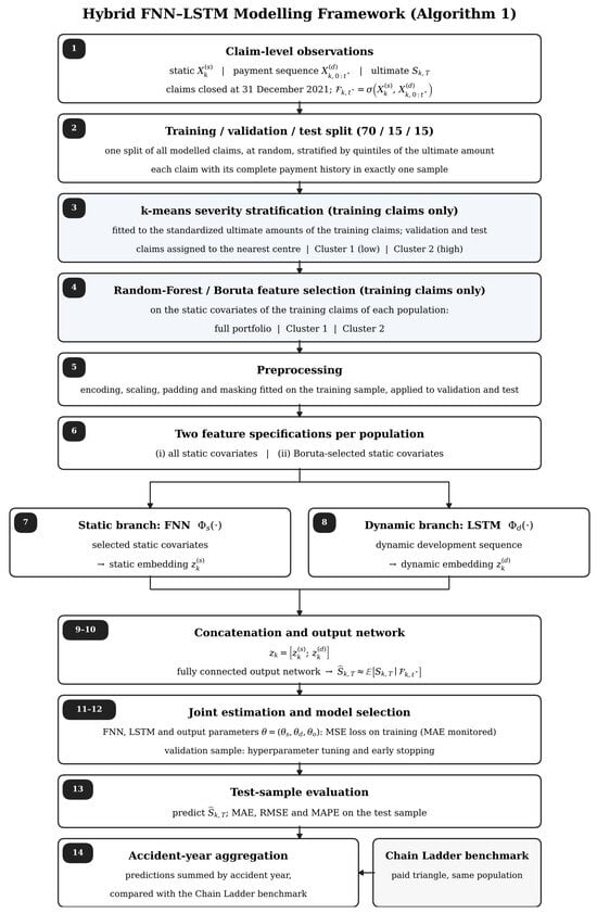
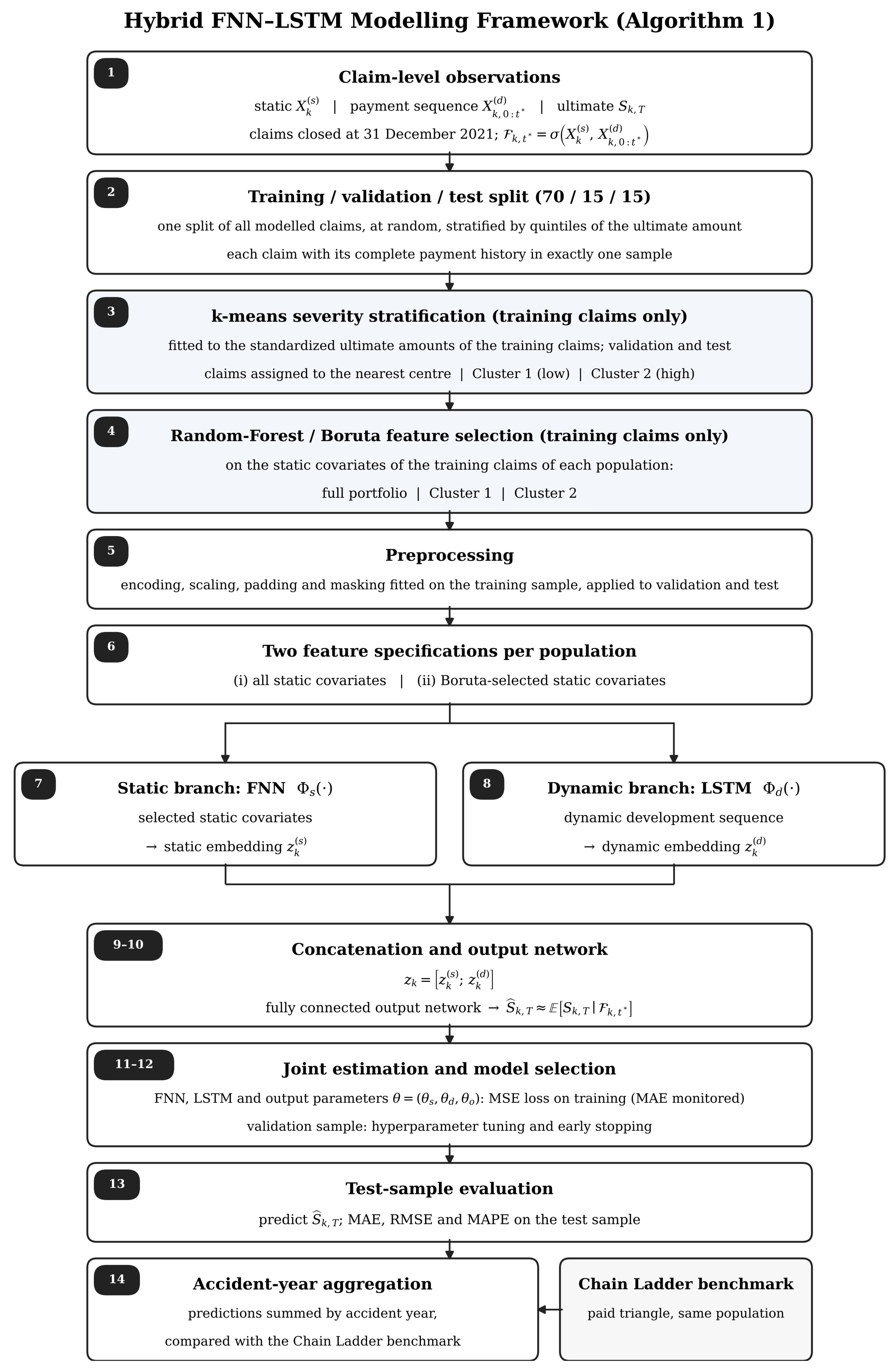
The overall information structure, the hybrid model architecture, and the modelling workflow are summarised in Figure 1, and the individual steps of the procedure are listed in Algorithm 1.
| Algorithm 1. Integrated hybrid FNN–LSTM reserving procedure |
|
Figure 1.
Modelling framework for individual-claim-level loss reserving, from the claim-level information set to the out-of-sample evaluation, showing the severity stratification and feature-selection steps and the hybrid FNN–LSTM architecture, together with the chain-ladder benchmark. The numbers in the boxes refer to the steps of Algorithm 1, and the arrows show the order in which the steps are carried out.
2.6. Evaluation Criteria
Model performance is evaluated at the individual-claim level and after aggregation by accident year. For a test sample of size , the mean absolute error is
The root mean squared error is
The mean absolute percentage error is
At the accident-year level, let denote the set of claims belonging to accident year . The observed and predicted aggregate ultimate losses are
These aggregated predictions are compared with the chain-ladder benchmark to assess whether claim-level modelling provides predictive gains at the portfolio-reserving level.
2.7. Data Simulation
To develop and evaluate the proposed claim-level reserving framework under controlled and reproducible conditions, this study relies on simulated data generated using the R-based model introduced by Wang and Wüthrich [20]. This framework constitutes a pedagogical implementation of the SynthETIC simulator originally proposed by Avanzi et al. [15] and is specifically designed for methodological investigations in microlevel loss reserving.
The simulator generates granular longitudinal claim data by explicitly modelling the key components of the claim process, including claim occurrence, claim severity, reporting and settlement delays, payment schedules, and the possibility of claim reopenings. Its modular structure allows full control over the data-generating mechanisms, including distributional assumptions, dependence structures, and temporal dynamics. This transparency is particularly important in the present context, as it ensures that model behaviour can be analysed independently of portfolio-specific idiosyncrasies and confidentiality constraints associated with proprietary insurance data.
The simulation is conducted relative to a fixed valuation cut-off date of 31 December 2021. At this cut-off, claims are classified as closed, reported but not settled (RBNS), or incurred but not reported (IBNR). To focus on the prediction of ultimate losses under complete development histories and to allow an unambiguous evaluation of predictive accuracy, the empirical analysis is restricted to closed claims. After applying this filtering step, the resulting dataset comprises 51,708 fully developed claims, of which 48,942 have at least one recorded payment and therefore enter the models when static and dynamic records are matched; these claims are partitioned into training, validation, and test samples as described in Section 3.1.
In addition to the core claim-development variables generated by the simulator, a set of contextual and demographic covariates is incorporated to reflect heterogeneity commonly observed in nonlife-insurance portfolios. These include policyholder characteristics (such as age, gender, education level, and occupation), vehicle-related attributes (including brand, vehicle type, engine power, and vehicle age), as well as geographical and environmental factors (such as region and weather conditions). Covariates are generated using a combination of uniform distributions and empirical proportions derived from publicly available data sources, ensuring plausible variability while maintaining full control over the underlying data-generating process.
Overall, the simulated dataset provides a transparent and flexible testing environment for assessing the interaction between feature selection, claim segmentation, and hybrid deep-learning architectures in a microlevel reserving setting. It also enables a clear and reproducible evaluation of model performance that would be difficult to achieve using proprietary data. However, the results should be interpreted as a controlled methodological assessment rather than definitive evidence of performance on real insurance portfolios.
3. Results
3.1. Model Implementation and Experimental Design
The empirical evaluation of the proposed hybrid neural-network framework is conducted at both the individual-claim and portfolio levels using using Python 3.13 (Python Software Foundation, Wilmington, DE, USA) with TensorFlow 2.21 and Keras 3.15 (Google LLC, Mountain View, CA, USA), Keras Tuner 1.4.8, scikit-learn 1.9.1, and BorutaPy 0.4.3.. The experiment is organised as a two-factor design. The first factor is the modelling population, taken as the full portfolio or one of the two severity strata defined below; the second is the feature specification, taken as the full set of static covariates or the Boruta-selected subset. All six combinations are estimated, and the object of interest is the interaction between the two factors, that is, whether the value of covariate reduction depends on the severity regime to which it is applied.
To examine heterogeneity in claim severity, claims are stratified using the k-means algorithm applied to the standardised ultimate claim amounts of the training claims only. The number of clusters is chosen by the average silhouette width over C = 2, …, 10 on a random subsample of 5000 training claims (0.896 for C = 2, against at most 0.886 for C = 3, …, 10), and the final solution is fitted to the ultimate amounts of the 34,259 training claims, with the number of random starts and the iteration limit chosen to minimise the within-cluster sum of squares. The procedure yields two distinct claim-size regimes with centres 6159 and 92,327, separated by a threshold ultimate claim amount of 49,243; validation and test claims are then assigned to the nearest centre, so that they have no influence on the threshold. Of the 48,942 modelled claims, 47,539 fall into Cluster 1 and 1403 into Cluster 2. Cluster 1 contains low-severity, relatively homogeneous claims, while Cluster 2 captures high-severity claims characterised by greater volatility. All subsequent analyses are performed both on the full portfolio and separately within each cluster. Because cluster membership is determined from the ultimate claim amount, the stratum-specific results are conditional on a known severity regime: they compare the hybrid model with chain ladder within each regime, which is the purpose of the heterogeneity analysis, but they are not an estimate of the accuracy of a segmented reserving procedure applied at the valuation date, when cluster membership would itself have to be predicted. Fitting k-means to all 48,942 modelled claims instead would give a threshold of 50,323 and move only five of the 7342 test claims (0.07%) to the other stratum; over 20 random training–validation–test splits, the training-based threshold ranges from 48,408 to 53,246.
The partition is made once, before the stratification and the feature selection: the 48,942 modelled claims are shuffled and partitioned at random into training (70%; 34,259 claims), validation (15%; 7341), and test (15%; 7342) samples with a fixed random seed (42), stratified by quintiles of the ultimate claim amount so that the three samples have comparable severity distributions (two-sample Kolmogorov–Smirnov tests against the training sample give p > 0.3 in every population). Each severity stratum inherits this partition, with 33,281, 7120, and 7138 claims in Cluster 1 and 978, 221, and 204 claims in Cluster 2. The unit of the split is the claim: each claim is assigned, together with its static covariates and its complete payment history over all development periods, to exactly one sample, so that no part of a validation or test claim is seen during training.
The network architectures, training settings, and hyperparameter search spaces are detailed in Appendix A (Table A1), while the hyperparameters of the full-portfolio models and those selected for the severity-stratum models are reported in Table A2 and Table A4. Each configuration consists of a fully connected static branch, a single-layer LSTM dynamic branch, and an output network with one hidden layer followed by a linear output unit. All models are trained using MSE loss with the Keras default weight initialisation, and all scalers are fitted to the training claims only.
The full-portfolio model with all covariates uses 48 static units, 48 LSTM units, and 32 output-network hidden units, with ReLU activation and the Adam optimiser (learning rate 0.001), trained for 15 epochs with a batch size of 32; the same architecture is used for both feature specifications, without tuning. For the severity-stratum models, hyperparameters are selected through a random search of 20 configurations using validation MSE and a fixed seed (42). Each configuration is trained for up to 100 epochs with a batch size of 32 and early stopping after 10 epochs without improvement, restoring the best weights.
Each of the six configurations was estimated once owing to computational constraints, as hyperparameter tuning required training 20 networks per stratum configuration. The main findings rest on differences in test MAE between the two feature specifications within the same population: with all covariates, test MAE is about 49% lower than with the Boruta-selected covariates in the low-severity stratum (285.1 against 559.3) and about 33% lower in the high-severity stratum (4401 against 6555), but about 39% higher in the full portfolio (363.4 against 261.7), while at the accident-year level the errors of chain ladder are about two to 20 times those of the hybrid models ((Section 3.4)). However, single-run estimation does not allow variability due to random initialisation to be quantified. Smaller differences, such as the gap of about 14% between the accident-year MAEs of the two high-severity models (156,625 against 181,654), are therefore interpreted cautiously. Repeated initialisations and prediction averaging, as suggested by Richman and Wüthrich [21], are identified as future work.
3.2. Feature Relevance and Variable Selection
Feature relevance is assessed using the Boruta algorithm [17], applied to the training claims of the full portfolio and, separately, to the training claims of each severity stratum, so that validation and test claims play no role in the selection. The implementation uses a random-forest regressor on the ultimate claim amount with 100 trees and a maximum depth of 7, at most 100 iterations, and a fixed seed (42); a variable is retained when at least one of its encoded columns is confirmed.
The results are reported in Table 1, which summarises the static covariates identified as important for ultimate-loss prediction.
Table 1.
Static variables selected by the Boruta algorithm on the training claims.
The selected sets are small and differ across populations. The reporting delay is confirmed in the full portfolio and in the low-severity stratum, where policyholder age is also retained, whereas in the high-severity stratum, with only 978 training claims, the inflation rate is the only confirmed covariate. None of the accident- and reporting-date variables is confirmed in any population. These results motivate the comparison in Section 3.3 of models estimated with the full set of static covariates and with the reduced Boruta-selected sets.
Under these settings, restricting the Boruta selection to the training claims produces only minor differences. In the full portfolio, the reporting delay remains the only confirmed covariate. In the low-severity stratum, the reporting delay and policyholder age are selected in both cases, while the reporting year is confirmed only when all claims are included. In the high-severity stratum, Boruta confirms no covariate when all claims are used, whereas the training-only selection retains the inflation rate. The reporting delay is therefore the most robust predictor, confirmed under both selections in the full portfolio and in the low-severity stratum. By contrast, the date-related variables show limited stability, with no accident- or reporting-date variable confirmed on the training claims alone. Finally, given the small high-severity training sample (fewer than 1000 claims), the selection for this stratum should be interpreted cautiously and should not be taken as evidence of substantive predictor importance.
3.3. Individual-Claim-Level Predictive Performance
Individual-claim-level predictive accuracy is evaluated using MAE, RMSE, and MAPE, computed on the training, validation, and test samples.
Results are reported in Table 2, which is organised into three panels corresponding to the full portfolio and the two claim-size clusters.
Table 2.
Individual-claim prediction accuracy of the hybrid neural network.
The three panels of Table 2 reveal distinct patterns across modelling populations. Training and test errors are generally comparable across all six models, suggesting no clear evidence of overfitting. Higher validation errors, particularly in the high-severity stratum and in the full-portfolio RMSE, are largely attributable to a few exceptionally large claims (up to 635,116) in the validation sample: excluding the three largest validation claims brings the validation errors close to the training and test errors. Test errors therefore provide the primary basis for model comparison.
In the full portfolio (Panel A), the model using only the Boruta-selected reporting delay achieves a lower test MAE than the model using all covariates (261.7 against 363.4), with comparable MAPE values (23.9% against 23.2%). However, because the network architecture is fixed rather than independently tuned, this improvement may partly reflect easier estimation with fewer inputs rather than the absence of predictive information in the excluded variables. In contrast, the full covariate set performs substantially better in both severity strata (Panels B and C), where hyperparameters are tuned separately. Test MAE is lower with all covariates by approximately 49% in the low-severity stratum (285.1 against 559.3) and 33% in the high-severity stratum (4401 against 6555).
These differences suggest that Boruta selection, when restricted to training claims, may exclude relevant predictive information. In the underlying simulator, claim severity depends on policyholder age, accident date, and weekend occurrence, with the latter two effects applying only to specific claim types [20]. Yet, except for policyholder age in the low-severity stratum, Boruta does not confirm these variables using training claims alone. The main finding is therefore that the effectiveness of feature selection depends on both portfolio segmentation and network configuration. Consequently, dimensionality reduction and severity-based segmentation should be evaluated jointly rather than treated as independent preprocessing steps.
3.4. Accident-Year Aggregation and Benchmarking
To evaluate reserving performance at the portfolio level, individual-claim predictions are aggregated by accident year and compared with the traditional chain-ladder method. In every modelling population, the accident-year totals are formed from the model predictions for all claims, including those in the training and validation samples. Aggregated performance metrics are reported in Table 3.
Table 3.
Accident-year aggregated prediction accuracy.
Across the full portfolio and the two clusters, the hybrid neural-network models achieve lower aggregate prediction errors than the chain-ladder benchmark in this simulated portfolio. The differences are especially visible for recent accident years and high-severity claims, where aggregate development factors are more sensitive to heterogeneity and incomplete development. Chain ladder is fitted here to the run-off triangle formed by aggregating, by accident year and development year, the same claims used to estimate the neural-network models; because the analysis is restricted to fully developed claims, this triangle is not identical to the one an insurer would observe at the valuation date, and the reported chain-ladder errors should be read accordingly. These results should be interpreted within the scope of the present empirical design and not as evidence of universal dominance over all classical reserving methods.
Directional accuracy is further examined by comparing actual and predicted aggregate ultimate losses by accident-year group. Results are summarised in Table 4.
Table 4.
Difference between actual and predicted aggregate ultimate claims by accident-year group (actual minus predicted; negative values indicate that the predicted aggregate ultimate exceeds the actual value, i.e., overestimation).
3.5. Backtest at an Intermediate Valuation Date
The comparisons in Section 3.2, Section 3.3 and Section 3.4 use the complete payment history of each claim. To assess how much of the advantage of the hybrid model depends on this information, the evaluation was repeated at an intermediate valuation date, 31 December 2019 (development month 96), with the model inputs restricted to the payment information available at that date. The backtest includes the 43,350 claims reported by December 2019 and keeps their allocation to the training, validation, and test samples of Section 3.1 (30,384, 6471, and 6495 claims). The payment sequences end in December 2019, and the static inputs, either the training-only Boruta covariate of the full-portfolio model or all covariates, are complemented by five quantities observed at the valuation date: the number of development months, the months since reporting, an indicator of settlement by the valuation date, the logarithm of the amount paid to date, and the number of payments to date. The target remains the ultimate amount. At the valuation date, 86.3% of the claims are settled, but only 58.6% of those of accident year 2018 and 23.4% of those of accident year 2019 (Table A5). Two versions of the network are estimated for each feature set: the fixed architecture of Table A1, trained for up to 100 epochs with early stopping (patience 10), and a version tuned by the random search used for the severity strata (20 trials; Table A6). Chain ladder is fitted to the paid triangle of the same claims observed at December 2019 (accident years 2012–2019, volume-weighted development factors), so that both approaches use the same payment information. A naive benchmark that sets the ultimate equal to the amount paid to date is also reported.
The backtest is constructed in five steps. (i) Claim set: of the 48,942 closed claims with at least one payment, those reported by month 96 are retained; claims reported later are unknown at the valuation date and are excluded, so the backtest covers reported claims only. (ii) Truncation: for each retained claim, only the payment events dated up to month 96 are kept. As in Section 2.4, the dynamic input is the sequence of these events, each described by the amount paid and an open-claim indicator, zero-padded to 19 steps and passed through a masking layer; both channels are standardised with the mean and standard deviation of the observed steps of the training claims. (iii) Valuation-date quantities: the number of development months, the months since reporting, the settlement indicator (settlement month up to 96), the logarithm of one plus the amount paid to date, and the number of payments to date are computed from the truncated data and added to the static covariates, which are standardised with training-claim statistics. (iv) Estimation: the target is the ultimate amount, standardised with the training mean and standard deviation, and the predictions are transformed back to the original scale. The fixed network is trained with Adam (learning rate 0.001, batch size 32) for up to 100 epochs, with early stopping on the validation loss (patience 10) and restoration of the best weights; the tuned network uses the same early stopping within a random search of 20 trials, and the trial with the lowest validation loss is retained. (v) Benchmarks: the chain-ladder triangle is built from the payments of the same retained claims, with accident years 2012–2019 in rows and calendar years of payment up to 2019 in columns; volume-weighted development factors are applied to the latest diagonal without a tail factor. Claim-level errors are computed on the test claims, and accident-year totals are formed over all retained claims, as in Section 3.4.
Table 5 reports the claim-level errors. For a claim settled by December 2019, the ultimate equals the amount paid to date, which is one of the inputs; the networks are not constrained to return it, and they are therefore also reported with their predictions for settled claims replaced by the amount paid. The informative comparison concerns the 932 test claims still open at the valuation date. For these claims the errors are much larger than for the test sample as a whole (MAE between 7731 and 8189), and the gain over the paid-to-date benchmark (MAE 9120) is modest, between 10% and 15%. The MAPE of the networks on open claims is about 200% or more because some of these claims are strongly overpredicted relative to their ultimate, whereas the paid-to-date benchmark never exceeds the ultimate, so its MAPE stays below 100%. On the full test sample, the paid-to-date benchmark has a lower MAE than every network used for all claims (1309 against 1481–1835), but a higher MAE than every network once settled claims are set at their paid amount (1109–1175).
Table 5.
Claim-level prediction errors in the backtest at December 2019.
Table 6 aggregates the predictions by accident year. Chain ladder overestimates the aggregate ultimate of accident years 2018–2019 by 40.53M, mostly in accident year 2019 (by 95% of the actual value; Table A5), while the paid-to-date benchmark falls short by 45.28M. The networks used for all claims deviate by 0.81M to 6.75M for these two years, but some of them deviate by more than 10M for the mature accident years 2012–2015, where the amounts paid are already close to the ultimate. Setting settled claims at their paid amount removes most of this error: the deviations for 2012–2015 fall to 0.33M or less, the accident-year MAPE of the four networks lies between 2.09% and 3.01%, against 16.49% for chain ladder, and the 2018–2019 deviations lie between 1.16M and 6.08M. The overestimation by chain ladder has in part the same origin as in Section 3.4: the evaluated claims are still those settled by the final valuation date, so recent accident years contain proportionally more quickly settled claims than the older years from which the development factors are estimated. Claims of accident years 2018–2019 reported after December 2019, which the development factors implicitly project but which are not in the evaluated set, amount to 9.0M of ultimate and explain only a small part of the difference.
Table 6.
Accident-year accuracy in the backtest at December 2019: MAPE across accident years and difference between actual and predicted aggregate ultimate claims by accident-year group (actual minus predicted).
The ranking of the two feature sets is not stable. When the networks predict all claims, all covariates give lower errors than the Boruta covariate with the fixed architecture (test MAE 1481.2 against 1835.1; accident-year MAPE 3.39% against 7.95%), whereas, after tuning, the Boruta covariate does (test MAE 1528.1 against 1703.9; accident-year MAPE 3.12% against 6.71%). Once settled claims are set at their paid amount, the accident-year ranking reverses in both cases (fixed architecture: 2.09% for the Boruta covariate against 2.51% for all covariates; tuned: 3.01% against 2.79%), and the four networks differ by less than one percentage point. Because each configuration was estimated once (Section 3.1), these differences between network versions are not interpreted further. What the backtest does show is that the accident-year advantage of the hybrid models over chain ladder does not depend on access to the complete payment history, whereas their claim-level gain over the amount paid to date is modest for claims that are still open.
4. Discussion
4.1. Interpretation of the Aggregate Results
Table 4 shows that, for early accident years, where claim development is largely complete, the chain-ladder method yields reasonable aggregate estimates, particularly within stable claim-size segments. However, for more recent accident years characterised by incomplete development, chain ladder exhibits systematic overestimation (negative entries in Table 4; for accident years 2019–2021 in the full portfolio, the chain-ladder ultimates exceed the actual values by 62.79M), with the effect being most pronounced in the low-severity stratum in absolute terms and in the high-severity stratum relative to its size. The direction of this error is a consequence of the design: because only claims closed by the valuation date are retained, the triangle for recent accident years contains only quickly settled claims, whereas the development factors are estimated from older accident years whose slowly settling claims have also closed; applying these factors to recent accident years therefore projects development that the retained claims will not have. In contrast, the hybrid neural network produces substantially smaller aggregate deviations that vary little across accident-year cohorts. In the full portfolio, both hybrid models underestimate the total of every accident year, by about 1% in most years with the single Boruta-selected covariate and by 3–6% with all covariates (Table A3); in the two strata, the models with all covariates deviate by less than 2M in every accident-year group. Part of this advantage reflects the design: the hybrid model observes the complete payment history of each closed claim, whereas chain ladder projects further development onto accident years whose claims are already complete. The backtest of Section 3.5 indicates how large this part is: when both approaches use only the payments made up to December 2019, the hybrid models still deviate much less than chain ladder for the two most recent accident years (by at most 6.75M, against 40.53M), but on the claims still open at that date their MAE (7731 to 8189) is about five times their MAE on the whole test sample (1481 to 1835; Table 5), and their gain over the amount paid to date on these claims is between 10% and 15%. The difference arises because most test claims are already settled at the valuation date, so their ultimate is largely determined by the payments observed, whereas the open claims are still developing and their remaining payments must be predicted; the open claims are therefore much harder to predict, and the overall test MAE understates the error on them. These findings are consistent with well-documented practical reserving challenges for immature accident years and long-tailed business lines, as discussed by Hindley [22].
The improved performance of the hybrid FNN–LSTM framework can be understood from an actuarial perspective. Chain ladder is based on aggregated accident-year and development-year information and therefore summarises claim development through average portfolio-level patterns. This structure is effective when the portfolio is homogeneous and development patterns are stable, but it may be less reliable for heterogeneous portfolios or immature accident years. In contrast, the proposed model uses individual-claim-level information. The feedforward component captures nonlinear effects of static covariates, which in the full covariate set include accident and reporting timing as well as policyholder and claim characteristics, and in the Boruta-selected sets are reduced to the reporting delay, policyholder age, or the inflation rate, while the LSTM component summarises the observed sequential development of each claim. The severity stratification further separates low-severity claims from more volatile high-severity claims, reducing the risk that a single aggregate development pattern is imposed on claims with different behaviour. Therefore, the observed improvement is not simply due to the use of a more complex algorithm, but to the model’s ability to combine claim-level covariates, development history, and severity heterogeneity within a unified reserving framework.
4.2. Synthesis
Taken together, the results reported in Table 1, Table 2, Table 3 and Table 4 support a narrower conclusion than a general claim of superiority of deep learning in reserving. Within the design considered here, the hybrid FNN–LSTM framework predicts ultimate amounts for fully developed claims more accurately than the aggregate benchmark, and it does so by combining temporal claim development with static contextual information. More informative than the overall gain, however, is its distribution across the portfolio. The covariate sets selected in Table 1 are small and differ across populations, the effect of feature selection in Table 2 depends on the population and on whether the network is tuned, and the aggregate differences in Table 3 and Table 4 are concentrated in recent accident years. The consistent element across the three tables is that the value of each modelling component, including feature selection, depends on the modelling population and on how the network is estimated, which argues for evaluating segmentation, feature selection, and model tuning jointly, and against reporting a single portfolio-level performance figure for methods of this kind.
4.3. Limitations and Scope
The conclusions of this study are subject to three main limitations. First, the analysis is restricted to claims closed at the final valuation date, so the RBNS and IBNR components that make up the reserve in practice are excluded, and the study is a predictive benchmark rather than an operational reserving exercise. The evaluation is also not a forward-looking forecast. In the main analysis the hybrid model sees the complete payment history of each claim, and the partition into training, validation, and test samples is random at the claim level, so every accident year appears in all three samples and extrapolation to unseen accident years is not tested. The backtest in Section 3.5 restricts the model inputs to the payments made up to December 2019, but it still relies on the final ultimate amounts of the claims for training, so it is not a fully operational forecast, and it examines the development stage at which a prediction is made only at a single valuation date (Table 5 and Table A5).
Second, the results are obtained on simulated data and compared with a single benchmark, chain ladder. Real portfolios include features the simulation abstracts from, such as reporting irregularities, inflation, and case-reserve revisions, and other methods such as Bornhuetter–Ferguson or claim-level generalised linear models are not compared.
Third, each configuration is estimated once, so small differences between configurations should not be overinterpreted (Section 3.1). In addition, the severity strata are assigned using the ultimate amount, so the stratum results are conditional on a known severity regime; the full-portfolio results are not affected.
5. Conclusions
This paper develops a hybrid neural-network framework for individual-claim reserving in nonlife insurance that integrates static claim characteristics and dynamic development information within a unified conditional-expectation formulation and evaluates it under controlled conditions on fully developed claims. The proposed architecture combines feedforward neural networks (FNNs) for time-invariant covariates with long short-term memory (LSTM) networks for sequential claim development, thereby providing a flexible nonlinear estimator of ultimate claim amounts at the microlevel. The study is framed as a structured assessment of how the components of such a framework interact, rather than as a proposal for a new modelling paradigm.
The empirical analysis is conducted on a synthetic portfolio of 51,708 individual claims generated under a transparent simulation framework designed to replicate realistic accident, reporting, and payment dynamics. To address claim heterogeneity and improve model interpretability, the hybrid architecture is complemented by random-forest-based feature selection and a k-means stratification by claim severity, both fitted to the training claims only. The results show that feature relevance and predictive performance differ across claim-size regimes, and that the small covariate sets obtained by training-only feature selection do not improve the tuned stratum models.
At the individual-claim level, training and test errors are close in every modelling population, so that none of the models shows signs of overfitting; the full covariate set gives the lowest test MAE in both severity strata, whereas the single Boruta-selected covariate gives the lowest test MAE in the untuned full-portfolio model. Because accuracy was not evaluated by development age, the study does not establish stability across development horizons. At the aggregate level, benchmarking against the chain-ladder method highlights limitations of aggregation-based reserving approaches in heterogeneous and partially developed portfolios. While chain ladder performs adequately for early accident years and stable claim segments, it overestimates the ultimates of recent accident years in the simulated portfolio, particularly, in relative terms, in high-severity regimes. In contrast, the hybrid framework yields smaller aggregate deviations across accident-year cohorts under the empirical setting considered in this study.
Taken together, the results suggest that hybrid deep-learning models structured around the actuarial information set can predict ultimate claim amounts more accurately than chain ladder in this retrospective setting, and that the value of feature selection cannot be judged independently of the modelling population and of how the model is estimated. Restricted to the training claims, Boruta retains only one or two covariates; these reduced sets are beneficial only for the untuned full-portfolio model, whereas in both severity strata, where the networks are tuned, the full covariate set yields a clearly lower test MAE. This is the study’s main methodological message: feature selection, segmentation, and model tuning should be evaluated jointly, because evaluating any one of them in isolation can give a misleading picture of its value. A backtest at December 2019, in which the networks and chain ladder use only the payments made up to that date, confirms the accident-year advantage of the hybrid models, while showing that their claim-level gain over the amount paid to date is modest for claims still open at that date. The scope of these conclusions is limited by the design described in Section 4.3, and in particular by the restriction to fully developed claims. The proposed framework is not intended to replace traditional reserving methods, but to complement them by providing a flexible data-driven alternative and an additional source of actuarial insight.
Addressing the limitations set out in Section 4.3 defines the natural continuation of this work: repeating the backtest of Section 3.5 at several valuation dates and including claims that remain open; extending the framework to censored RBNS claims and IBNR estimation; predicting severity-cluster membership using information available at the valuation date; conducting out-of-time validation and assessing accuracy by development age; expanding classical benchmarks; evaluating robustness across multiple initialisations and quantifying predictive uncertainty; and validating the framework on real insurance portfolios. Within its stated scope, the present study shows that a hybrid neural architecture can be embedded coherently within the actuarial reserving framework, and that the interaction between segmentation, feature selection, and model tuning is a material design consideration for microlevel loss reserving.
Author Contributions
Conceptualisation, R.-M.H. and R.B.; methodology, R.-M.H., R.B. and S.A.; software, R.-M.H., R.B. and S.A.; validation, R.-M.H., R.B. and S.A.; formal analysis, R.-M.H. and R.B.; investigation, R.-M.H. and R.B.; data curation, R.-M.H. and S.A.; writing—original draft preparation, R.-M.H. and R.B.; writing—review and editing, R.-M.H. and R.B.; visualisation, R.-M.H., R.B. and S.A.; supervision, R.-M.H. and R.B. All authors have read and agreed to the published version of the manuscript.
Funding
This research received no external funding.
Data Availability Statement
The study uses synthetic data produced with the publicly available claim-simulation frameworks described in [15,20]. The simulation scripts and the generated datasets that support the reported results are available from the corresponding author upon request. No new empirical data were collected.
Acknowledgments
During the preparation of this manuscript, the authors used ChatGPT (GPT-5, OpenAI), Claude (Claude Opus 5.5, Anthropic), and Scopus AI (https://www.elsevier.com/products/scopus/scopus-ai (accessed on 12 November 2026), Elsevier) for the purposes of language refinement, structural organisation, and preliminary literature exploration. The authors have reviewed and edited the output and take full responsibility for the content of this publication.
Conflicts of Interest
The authors declare no conflicts of interest.
Appendix A
Table A1 summarises the network architectures, preprocessing, and training settings; Table A2 reports the hyperparameters of the full-portfolio models; Table A3 disaggregates the aggregate deviations of the full-portfolio model by single accident year; Table A4 reports the hyperparameters selected by the random search for the severity-stratum models; Table A5 disaggregates the backtest of Section 3.5 by accident year; and Table A6 reports the hyperparameters selected for the tuned backtest models.
Table A1.
Network architecture, preprocessing, and training settings.
Table A2.
Hyperparameters of the full-portfolio models (both feature specifications).
Table A3.
Actual and predicted aggregate ultimate claims of the full-portfolio hybrid model (all features) by accident year.
Table A4.
Hyperparameters selected by the random search for the severity-stratum models.
Table A5.
Backtest at December 2019 by accident year: development at the valuation date and relative deviation of the predicted aggregate ultimates.
Table A6.
Hyperparameters selected by the random search for the tuned backtest models.
References
- Bornhuetter, R.L.; Ferguson, R.E. The actuary and IBNR. Proc. Casualty Actuar. Soc. 1972, 59, 181–195. [Google Scholar] [CrossRef] [Scilit]
- Harej, B.; Gächter, R.; Jamal, S. Individual Claim Development with Machine Learning; Report of the ASTIN Working Party; International Actuarial Association: Ottawa, ON, Canada, 2017. [Google Scholar]
- Gabrielli, A.; Wüthrich, M.V. An individual claims history simulation machine. Risks 2018, 6, 29. [Google Scholar] [CrossRef] [Scilit]
- Wüthrich, M.V. Machine learning in individual claims reserving. Scand. Actuar. J. 2018, 465–480. [Google Scholar] [CrossRef] [Scilit]
- Gabrielli, A.; Wüthrich, M.V. Back-testing the chain-ladder method. Ann. Actuar. Sci. 2019, 13, 334–359. [Google Scholar] [CrossRef] [Scilit]
- Gabrielli, A.; Richman, R.; Wüthrich, M.V. Neural network embedding of the over-dispersed Poisson reserving model. Scand. Actuar. J. 2020, 1–29. [Google Scholar] [CrossRef] [Scilit]
- Bücher, A.; Rosenstock, A. Micro-level prediction of outstanding claim counts based on novel mixture models and neural networks. Eur. Actuar. J. 2023, 13, 55–90. [Google Scholar] [CrossRef] [Scilit] [PubMed]
- Somaratne, L.H. Ultimate loss reserve forecasting using bidirectional LSTMs. Casualty Actuar. Soc. E-Forum 2022, Summer. Available online: https://forum.casact.org/article/37953-ultimate-loss-reserve-forecasting-using-bidirectional-lstms (accessed on 12 November 2026).
- Feng, Y.; Li, S. Advancing the use of deep learning in loss reserving: A generalized DeepTriangle approach. Risks 2024, 12, 4. [Google Scholar] [CrossRef] [Scilit]
- Chaoubi, I.; Besse, C.; Cossette, H.; Côté, M.-P. Micro-level reserving for general insurance claims using a long short-term memory network. Appl. Stoch. Models Bus. Ind. 2023, 39, 382–407. [Google Scholar] [CrossRef] [Scilit]
- Schneider, J.C.; Schwab, B. Advancing loss reserving: A hybrid neural network approach for individual claim development prediction. J. Risk Insur. 2025, 92, 389–423. [Google Scholar] [CrossRef] [Scilit]
- Avanzi, B.; Li, Y.; Wong, B.; Xian, A. Ensemble distributional forecasting for insurance loss reserving. Scand. Actuar. J. 2024, 971–1012. [Google Scholar] [CrossRef] [Scilit]
- Richman, R.; Wüthrich, M.V. From chain-ladder to individual claims reserving. arXiv 2026, arXiv:2602.15385. [Google Scholar]
- Avanzi, B.; Richman, R.; Wong, B.; Wüthrich, M.V.; Xie, Y. Reinforcement learning for micro-level claims reserving. arXiv 2026, arXiv:2601.07637. [Google Scholar]
- Avanzi, B.; Taylor, G.; Wang, M.; Wong, B. SynthETIC: An individual insurance claim simulator with feature control. Insur. Math. Econ. 2021, 100, 296–308. [Google Scholar] [CrossRef] [Scilit]
- Breiman, L. Random forests. Mach. Learn. 2001, 45, 5–32. [Google Scholar] [CrossRef] [Scilit]
- Kursa, M.B.; Rudnicki, W.R. Feature selection with the Boruta package. J. Stat. Softw. 2010, 36, 1–13. [Google Scholar] [CrossRef] [Scilit]
- Hochreiter, S.; Schmidhuber, J. Long short-term memory. Neural Comput. 1997, 9, 1735–1780. [Google Scholar] [CrossRef] [Scilit] [PubMed]
- Gneiting, T. Making and evaluating point forecasts. J. Am. Stat. Assoc. 2011, 106, 746–762. [Google Scholar] [CrossRef] [Scilit]
- Wang, M.; Wüthrich, M.V. Individual Claims Generator for Claims Reserving Studies: Data Simulation.R; SSRN Working Paper, 2022. Available online: https://ssrn.com/abstract=4127073 (accessed on 12 November 2026).
- Richman, R.; Wüthrich, M.V. Nagging predictors. Risks 2020, 8, 83. [Google Scholar] [CrossRef] [Scilit]
- Hindley, D. Claims Reserving in General Insurance; Cambridge University Press: Cambridge, UK, 2017. [Google Scholar] [CrossRef] [Scilit]

Disclaimer/Publisher’s Note: The statements, opinions and data contained in all publications are solely those of the individual author(s) and contributor(s) and not of MDPI and/or the editor(s). MDPI and/or the editor(s) disclaim responsibility for any injury to people or property resulting from any ideas, methods, instructions or products referred to in the content. |
© 2026 by the authors. Licensee MDPI, Basel, Switzerland. This article is an open access article distributed under the terms and conditions of the Creative Commons Attribution (CC BY) license.