


Abstract
Actuator placement based on the degree of disturbance rejection (DoDR) typically assumes a prescribed disturbance covariance, although the actual disturbance statistics may be uncertain. This paper develops a controller-independent robust DoDR-based actuator-placement framework for asymptotically stable and controllable linear time-invariant systems under disturbance covariance uncertainty. By introducing an auxiliary Lyapunov equation, the steady-state DoDR is expressed as a linear function of the disturbance covariance, allowing its worst-case value to be characterized through the support function of a prescribed uncertainty set. Closed-form expressions are derived for two representative uncertainty models: total additional disturbance-power uncertainty and spatial disturbance-power uncertainty. Numerical examples using a five-mass spring–damper system demonstrate that the optimal actuator placement can change when disturbance covariance uncertainty is taken into account. Furthermore, closed-loop evaluations using LQR controllers show that the actuator configuration selected by the robust DoDR can provide favorable worst-case disturbance-rejection performance under uncertain disturbance locations. These results demonstrate the usefulness of the proposed framework for evaluating disturbance-rejection capabilities and selecting actuator configurations without requiring prior feedback-controller design.
Keywords:
degree of disturbance rejection (DoDR); robust actuator placement; disturbance covariance uncertainty; controllability Gramian; robust optimization MSC:
93B05
1. Introduction
The degree of controllability (DoC) provides a quantitative characterization of how easily a controllable system can be driven by control inputs. Representative approaches include the controllability norm [1], PBH/eigenvector-based measures [2], modal controllability measures [3], and bounded-input-based definitions [4]. Among these approaches, Gramian-based measures are particularly useful because of their direct relationship with the minimum control energy [5]. Quantitative controllability concepts have subsequently been extended to various system classes and design problems, including descriptor systems [6], nonlinear systems [7], and dynamical networks [8,9]. These developments have established DoC-related measures as useful tools not only for evaluating controllability but also for system configuration and design.
One of the important applications of quantitative controllability is actuator placement or allocation. Controllability- and Gramian-based criteria have been widely used to determine effective actuator locations in flexible structures [10,11], unstable systems [12], and structural topology optimization [13]. Related formulations have also been developed for actuator placement in rotating flexible structures under varying operating conditions [14,15]. From the perspective of extending the underlying controllability metric, a steady-state DoC measure applicable to linear unstable systems was developed in [16], and a recent formulation for linear systems with semi-stable modes enables actuator allocation while accounting for marginally stable dynamics [17]. These studies demonstrate the usefulness of quantitative controllability as a controller-independent criterion for comparing candidate actuator configurations.
External disturbances provide another important consideration in control configuration and actuator placement. Early studies addressed input selection and actuator placement for disturbance rejection using frequency-domain or closed-loop performance measures [18,19]. A disturbance sensitivity Gramian was introduced for actuator placement in active vibration control with known disturbances [20], and related robust actuator-placement formulations were subsequently investigated under uncertainty in the spatial distribution of disturbances [21]. These approaches include both Gramian-based placement measures and criteria that depend on a prescribed or jointly optimized feedback controller. In contrast, a controllability measure based on an idealized minimum-energy criterion for disturbance rejection was proposed in [22]. This measure, subsequently referred to as the degree of disturbance rejection (DoDR), provides a controller-independent characterization of the inherent disturbance-rejection capability of a system. Related disturbance-aware controllability measures have also been applied to wind-turbine design and output-regulation problems [23,24,25].
The applicability of DoDR has recently been extended beyond conventional asymptotically stable systems. Steady-state disturbance-rejection controllability has been investigated for linear unstable systems [26], undamped flexible structures [27], and systems containing rigid-body modes [28]. However, existing DoDR-based formulations generally evaluate disturbance-rejection controllability for prescribed disturbance statistics. Consequently, an actuator configuration selected using a nominal disturbance covariance may become unfavorable when the actual disturbance intensity, spatial distribution, or correlation differs from the assumed covariance.
In practical applications, disturbance covariance information may be incomplete or uncertain. For example, a nominal covariance may be available together with a bound on additional disturbance power, or only the total disturbance power and possible disturbance locations may be known. This leaves open how covariance uncertainty should be incorporated directly into the DoDR criterion for actuator placement while preserving its controller-independent interpretation. Unlike earlier DoDR extensions that address different stability classes, the present study focuses on covariance uncertainty itself. Restricting the analysis to asymptotically stable systems permits the use of standard steady-state Lyapunov equations without the additional complications of divergent Gramians. Accordingly, this study considers asymptotically stable LTI systems, for which the conventional steady-state DoDR is well defined, and develops a robust DoDR framework in which actuator configurations are evaluated according to the worst-case disturbance-rejection controllability over a prescribed covariance uncertainty set.
Table 1 compares representative actuator-placement approaches in terms of their strengths and limitations. In particular, Demetriou and Moghani [21] consider spatial disturbance uncertainty and present both a controller-independent controllability-Gramian screening criterion and feedback-dependent placement criteria. In contrast, the present study extends the original DoDR [22] to disturbance covariance uncertainty while retaining a controller-independent placement criterion.
Table 1.
Strengths and limitations of representative actuator-placement approaches.
The main contributions of this study are summarized as follows:
- A controller-independent robust DoDR-based actuator-placement problem is formulated under disturbance covariance uncertainty.
- A covariance-linear representation of the steady-state DoDR is derived, leading to a general support-function representation of the robust DoDR.
- Closed-form robust DoDR expressions are obtained for total additional disturbance-power and spatial disturbance-power uncertainty.
- Numerical examples demonstrate the actuator-placement characteristics of the proposed robust DoDR framework.
Gramian-based actuator placement has been investigated in flexible structures [10,20,21], and disturbance-aware controllability measures have been explored in wind-turbine applications [23]. These studies suggest potential engineering applications of the proposed framework, provided that suitable asymptotically stable LTI models and disturbance covariance uncertainty descriptions are available. Since application-specific modeling and experimental validation are beyond the scope of this study, the proposed framework is illustrated using a simplified five-mass spring–damper system.
The remainder of this paper is organized as follows. Section 2 reviews the steady-state DoDR and formulates the nominal and robust actuator-placement problems. Section 3 derives the covariance-linear representation and develops the robust DoDR formulation, including closed-form solutions for representative covariance uncertainty sets. Section 4 presents numerical examples using a five-mass spring–damper system and illustrates the closed-loop characteristics of representative actuator configurations through LQR simulations. Finally, Section 5 concludes the paper.
2. Preliminaries and Problem Formulation
This section presents the preliminaries and problem formulation required to develop the proposed actuator-placement framework under disturbance covariance uncertainty. First, the steady-state disturbance-rejection controllability metric is briefly reviewed as the basis for evaluating the inherent disturbance-rejection capability of a given actuator configuration. Then, the conventional nominal actuator-placement problem with a known disturbance covariance is introduced, followed by the formulation of the robust actuator-placement problem in which the disturbance covariance belongs to a prescribed uncertainty set.
2.1. Steady-State Disturbance-Rejection Controllability
Consider a controllable linear time-invariant (LTI) system described by
where , , and denote the state, control input, and disturbance vectors, respectively. The matrices A, B, and D are constant matrices of appropriate dimensions. The disturbance is assumed to be a zero-mean Gaussian white-noise process satisfying
where S is the covariance intensity matrix of the idealized white-noise process, rather than a pointwise covariance matrix. Throughout this paper, the term “disturbance covariance” is used as shorthand for this covariance intensity.
The disturbance-rejection controllability metric proposed in [22], subsequently referred to as the degree of disturbance rejection (DoDR) in related studies [26,27,28], is defined through an idealized disturbance-preview minimum-energy problem:
subject to , , and the dynamics in (1). The terminal constraint is imposed almost surely, and the minimization is over square-integrable control inputs that may depend on the complete disturbance realization over . For each realization, let denote the disturbance-induced terminal state under . The minimum-energy input satisfying the terminal constraint is
where denotes the finite-horizon controllability Gramian, defined by
The input in (4) depends on , which is generally unknown before , and is, therefore, noncausal. For each disturbance realization, its control energy equals . Taking the expectation yields the closed-form DoDR [22]:
where the covariance of the disturbance-induced terminal state and the disturbance Gramian satisfy
Consequently, the DoDR is a theoretical preview-based minimum-energy benchmark rather than the energy consumed by an implementable causal feedback controller. A smaller value of indicates a lower idealized minimum energy and, in this sense, corresponds to better disturbance-rejection controllability.
In this study, A is assumed to be Hurwitz, and is assumed to be controllable for every admissible actuator configuration considered. Under these assumptions, the finite-horizon Gramians in (5) and (7) converge to unique steady-state limits, denoted by and , respectively. These steady-state Gramians satisfy the algebraic Lyapunov equations [29]
These equations follow directly from the integral definitions of the Gramians. Since A is Hurwitz, as , and
The same calculation with replaced by yields the corresponding relation for . Consequently, the steady-state DoDR is expressed as
The metric in (11) provides a time-independent measure of the disturbance-rejection capability associated with a given actuator configuration without specifying a particular feedback controller. In the following subsection, this metric is used to formulate nominal and robust actuator-placement problems according to whether the disturbance covariance is known exactly or belongs to an uncertainty set.
2.2. Nominal and Robust Actuator-Placement Problems
Let the set of admissible actuator configurations be defined as
where each represents a candidate actuator configuration. As assumed in the previous subsection, is controllable for every . Throughout this study, the system matrix A and disturbance distribution matrix D are fixed, whereas the actuator configuration B is selected from .
When a nominal disturbance covariance intensity is prescribed, the conventional DoDR-based actuator-placement problem can be formulated as
This formulation determines the actuator configuration that minimizes the idealized minimum-energy criterion for disturbances characterized by the prescribed nominal covariance . Its performance, however, depends on how accurately represents the actual disturbance statistics.
To account for uncertainty in the disturbance statistics, suppose that the actual disturbance covariance intensity S is unknown but belongs to a prescribed uncertainty set
where
and is assumed to be a nonempty compact convex set. Thus, is the nominal intensity, S denotes a possible actual intensity, and collects all admissible covariance intensities. The robust DoDR associated with an actuator configuration B and the corresponding robust actuator-placement problem are then defined as
Accordingly, minimizes the worst-case value of the preview-based minimum-energy criterion over all covariance matrices contained in . Unlike the nominal formulation in (13), this formulation does not rely on a single prescribed covariance matrix and, therefore, explicitly accounts for uncertainty in the disturbance statistics.
The robust formulation in (17) requires characterizing the worst-case DoDR over all disturbance covariances consistent with the available uncertainty information. However, the dependence of the DoDR on the covariance matrix S is implicit in (11), since S enters through the disturbance Gramian defined by the Lyapunov equation (9). In the next section, this dependence is characterized explicitly, allowing the worst-case DoDR to be analyzed directly over the covariance uncertainty set and enabling exact robust characterizations for representative forms of covariance uncertainty.
3. Robust Disturbance-Rejection Controllability Under Covariance Uncertainty
This section develops a robust characterization of disturbance-rejection controllability when the disturbance covariance is not known exactly but is only known to belong to the uncertainty set . To this end, the dependence of the steady-state DoDR on the covariance matrix is first expressed explicitly, leading to a general support-function representation of the robust DoDR. Closed-form solutions are then derived for representative covariance uncertainty sets, followed by a general characterization of the covariance structures at which the worst-case DoDR can be attained.
3.1. Covariance-Linear Representation of the DoDR
The steady-state DoDR in (11) depends on the disturbance covariance S through the disturbance Gramian , which is implicitly determined by the Lyapunov Equation (9). To expose this dependence explicitly, for a fixed actuator configuration , define an auxiliary matrix as the unique solution of
Since A is Hurwitz and , the solution exists uniquely and satisfies . Define
where depends on the system and actuator configuration but is independent of the disturbance covariance S. Because , is positive semidefinite and is positive definite if D has full column rank; in particular, is singular when D is rank deficient. The following theorem provides an explicit representation of the steady-state DoDR in terms of S.
Theorem 1.
Proof.
Theorem 1 shows that, for a fixed actuator configuration, the steady-state DoDR is a linear function of the disturbance covariance matrix. In particular, if and , then
Thus, the diagonal element characterizes the sensitivity of the DoDR to the disturbance variance in the ith channel, whereas the off-diagonal elements characterize the influence of correlations between disturbance channels. Since , the resulting DoDR is nonnegative for every admissible covariance matrix . This explicit linear dependence on S provides the basis for characterizing the worst-case DoDR directly over the covariance uncertainty set in the following subsection.
3.2. General Robust DoDR Formulation
Using the covariance-linear representation established in Theorem 1, the robust DoDR defined in (16) can be expressed directly in terms of the covariance uncertainty set. For symmetric matrices X and Y of the same dimension, define the inner product
Since both and S are symmetric, . The support function of the covariance uncertainty set [30] is defined as
Because is nonempty and compact, the maximum in (23) is attained and is finite.
Corollary 1.
For a fixed actuator configuration , the robust DoDR over the covariance uncertainty set is given by
Consequently, the robust actuator-placement problem in (17) can be equivalently expressed as
Proof.
Corollary 1 separates the effects of the system and actuator configuration from the description of the disturbance uncertainty. Specifically, characterizes how a given actuator configuration responds to variations in the disturbance covariance, whereas describes the available information regarding the possible disturbance statistics. Therefore, once is determined for a given actuator configuration, its worst-case disturbance-rejection controllability is completely characterized by the support function of evaluated at .
A useful translated representation arises when a nominal covariance is included in the covariance uncertainty set. In this case, the uncertainty set can be written as
where is a nonempty compact convex set of symmetric perturbation matrices containing , and for every . Here, denotes the deviation of an admissible covariance intensity S from the nominal intensity , whereas is the set of admissible perturbations. Combining Theorem 1 with Corollary 1, the robust DoDR is expressed as
Equation (28) separates the nominal DoDR from the worst-case deviation associated with the admissible covariance perturbations. Because , the nominal covariance itself is admissible and . Therefore, .
The general representation in (24) does not require a specific form of the covariance uncertainty set. Once the available information on the disturbance covariance is represented by a particular set , the corresponding robust DoDR is obtained by evaluating the support function of at . In the following subsection, closed-form expressions are derived for representative covariance uncertainty sets relevant to robust actuator placement.
3.3. Closed-Form Solutions for Representative Covariance Uncertainty Sets
The general robust formulation in (24) expresses the robust DoDR as the support function of the covariance uncertainty set evaluated at . Therefore, a closed-form robust DoDR can be obtained whenever the corresponding support function admits an explicit expression. This subsection considers two representative forms of covariance uncertainty describing different levels of available disturbance information. The first case assumes that a nominal covariance is available while only the total amount of additional disturbance power is bounded. The second case assumes that the total disturbance power is known, but its distribution among the disturbance channels is uncertain.
3.3.1. Total Additional Disturbance-Power Uncertainty
Suppose that the disturbance covariance is represented as
where the covariance perturbation belongs to the uncertainty set
Here, specifies an upper bound on the total additional disturbance power beyond that represented by the nominal covariance . Unlike the general perturbation model in (27), this uncertainty model imposes , so that the covariance uncertainty represents only additional disturbance power relative to . This model is appropriate when uncertainty adds covariance power to the nominal baseline, but excludes changes that cannot be represented by a positive-semidefinite addition, such as variations in inter-channel correlations at fixed channel variances or redistributions of existing disturbance power. From (28), the robust DoDR is determined by the support function .
Proposition 1.
For the uncertainty set in (30), the robust DoDR is
where denotes the largest eigenvalue of . For , a worst-case covariance perturbation can be chosen as
where is a unit eigenvector of associated with . If has multiplicity greater than one, the choice of is not unique, and the worst-case covariance perturbation need not be unique.
Proof.
Accordingly, the robust actuator-placement problem for this uncertainty model becomes
The first term in (33) represents the disturbance-rejection performance under the nominal covariance, whereas the second term represents the worst-case contribution associated with the admissible additional covariance power. The worst-case perturbation in (32) concentrates the additional disturbance power along the disturbance-space direction to which the DoDR is most sensitive. Since the disturbance enters the state equation through , this direction corresponds to the state-space disturbance direction .
3.3.2. Spatial Disturbance-Power Uncertainty
Consider the disturbance distribution matrix
where represents the ith disturbance channel. Suppose that the disturbance channels are uncorrelated and that the total disturbance power is known, whereas its distribution among the individual channels is uncertain. The corresponding covariance uncertainty set is defined as
where denotes the prescribed total disturbance power. No upper bounds are imposed on individual channel intensities, so the model permits all disturbance power to be concentrated in a single channel. Correlations between channels and channel-specific power bounds are not represented by this uncertainty set. According to Corollary 1, the robust DoDR for this uncertainty model is determined by the support function .
Proposition 2.
Let . For the spatial disturbance-power uncertainty set in (35), the robust DoDR is
A worst-case covariance matrix is
where denotes the ith standard basis vector in . If several diagonal entries attain the same maximum, the worst-case covariance is not unique; any nonnegative allocation of the total power γ among those maximizing channels is also optimal.
Proof.
By the definition of the support function in (23),
For every admissible allocation of the disturbance power,
The upper bound is attained by assigning the entire disturbance power to any channel satisfying
which corresponds to the covariance matrix in (37). Therefore, . Equation (36) then follows directly from (24). □
Since is common to all actuator configurations, the corresponding robust actuator-placement problem reduces to
Furthermore, from (19) and (34),
For a unit-power disturbance acting exclusively through the ith disturbance channel, the covariance matrix is , and Theorem 1 gives
Thus, directly represents the DoDR associated with a unit-power disturbance acting through the ith disturbance channel. Consequently, (38) selects the actuator configuration that minimizes the largest disturbance-rejection energy requirement among all admissible disturbance channels.
To clarify the distinction between the proposed robust DoDR and existing approaches to spatially robust actuator placement, consider the method of Demetriou and Moghani [21]. Their study considers uncertainty in the spatial distribution of disturbances and evaluates its influence on actuator placement through controllability-Gramian screening and closed-loop performance criteria. The integrated closed-loop approaches involve feedback-controller design for each candidate actuator location, and representative spatial disturbance distributions are examined numerically. In contrast, the proposed robust DoDR explicitly characterizes covariance uncertainty through a prescribed uncertainty set and provides a controller-independent worst-case placement criterion. In particular, the support-function representation in (24) yields closed-form solutions for the two covariance uncertainty models considered here, without requiring feedback-controller design.
The two uncertainty models considered above correspond to different types of incomplete disturbance information. The trace-bounded perturbation model allows the additional covariance power to be distributed along arbitrary directions in the disturbance space, including correlated combinations of disturbance channels, whereas the spatial uncertainty model assumes uncorrelated disturbance channels and considers uncertainty only in the allocation of a prescribed total disturbance power. Both models admit exact closed-form robust DoDR expressions through (24), whereas other nonempty compact convex covariance uncertainty sets can be treated by the same support-function formulation but may require numerical optimization. Moreover, the worst-case covariance in each case is attained at an extreme point of the corresponding uncertainty set. The following subsection shows that this common property is a general consequence of the covariance-linear representation of the DoDR.
3.4. Extreme-Point Interpretation of Worst-Case Covariance
The two closed-form results in the previous subsection exhibit a common structural property: the worst-case covariance can be chosen at an extreme point of the corresponding covariance uncertainty set. This property follows directly from the covariance-linear representation of the DoDR and a standard result in convex analysis.
Corollary 2.
Let be a nonempty compact convex covariance uncertainty set. For any fixed actuator configuration , there exists a worst-case covariance such that
where denotes the set of extreme points of .
Since is linear in S, the result follows from the standard extreme-point property of linear optimization over a nonempty compact convex set [31]. In the trace-bounded uncertainty model, this property is reflected by the rank-one worst-case perturbation . In the spatial uncertainty model, it is reflected by , which concentrates the total disturbance power in a single disturbance channel. Thus, the extreme covariance structures obtained in the two closed-form cases are manifestations of the covariance-linear dependence of the DoDR rather than isolated properties of the particular uncertainty models.
3.5. Computational Procedure and Numerical Considerations
The proposed procedure is applied to the admissible set , for which each pair is assumed to be controllable. An uncontrollable configuration is, therefore, excluded from , since its steady-state controllability Gramian is singular and the DoDR in (11) is undefined. The computational procedure for evaluating the robust DoDR and selecting an actuator configuration is summarized in Algorithm 1 and illustrated in Figure 1.
Figure 1.
Block diagram of the proposed robust DoDR-based actuator-placement procedure.
For a controllable but nearly uncontrollable configuration, may be ill-conditioned, making the evaluation of sensitive to numerical errors. Rather than excluding such configurations or assigning an arbitrary DoDR penalty, their numerical reliability should be assessed using the smallest eigenvalue and condition number of , together with checks of positive definiteness and the relative residuals of the two Lyapunov equations. Motivated by residual-based assessments of numerical matrix-equation solutions [32], we define the following normalized Frobenius residuals:
where denotes the Frobenius norm. Values close to zero indicate that the computed matrices satisfy their respective Lyapunov equations with small residuals relative to the individual equation terms, while larger values indicate greater equation inconsistency. However, small residuals alone do not guarantee small solution errors in ill-conditioned problems [33]. If numerical sensitivity is detected, the computed robust DoDR and actuator ranking should be reassessed using more accurate procedures or higher precision. Candidates whose scores cannot be evaluated reliably should be flagged rather than ranked using potentially inaccurate values.
Standard Schur-based methods can be used for the Lyapunov equations, and inverse-related operations can be implemented through linear system solves, although such procedures do not eliminate the effects of poor conditioning. The formulation also applies directly to multiple actuators through multicolumn input matrices B. For large-scale systems, specialized Lyapunov solvers are available, but the inverse-related computation and the evaluation of potentially many actuator configurations remain practical limitations [32].
4. Numerical Examples
This section presents numerical examples to demonstrate the actuator-placement characteristics of the proposed robust DoDR framework under disturbance covariance uncertainty. A five-mass spring–damper system is considered with multiple candidate actuator and disturbance locations, providing an interpretable benchmark for evaluating the proposed method before considering more complex engineering systems. First, the total additional disturbance-power uncertainty model is examined to illustrate how the optimal actuator placement can change as the uncertainty bound increases from the nominal case. Next, the spatial disturbance-power uncertainty model is considered to determine a robust actuator location when only the total disturbance power and the set of possible disturbance locations are known. Finally, the stationary LQR performance of all five configurations is evaluated, followed by time-domain simulations of representative configurations to illustrate their closed-loop disturbance responses.
4.1. Five-Mass Spring–Damper System
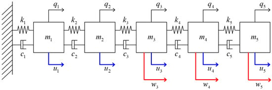
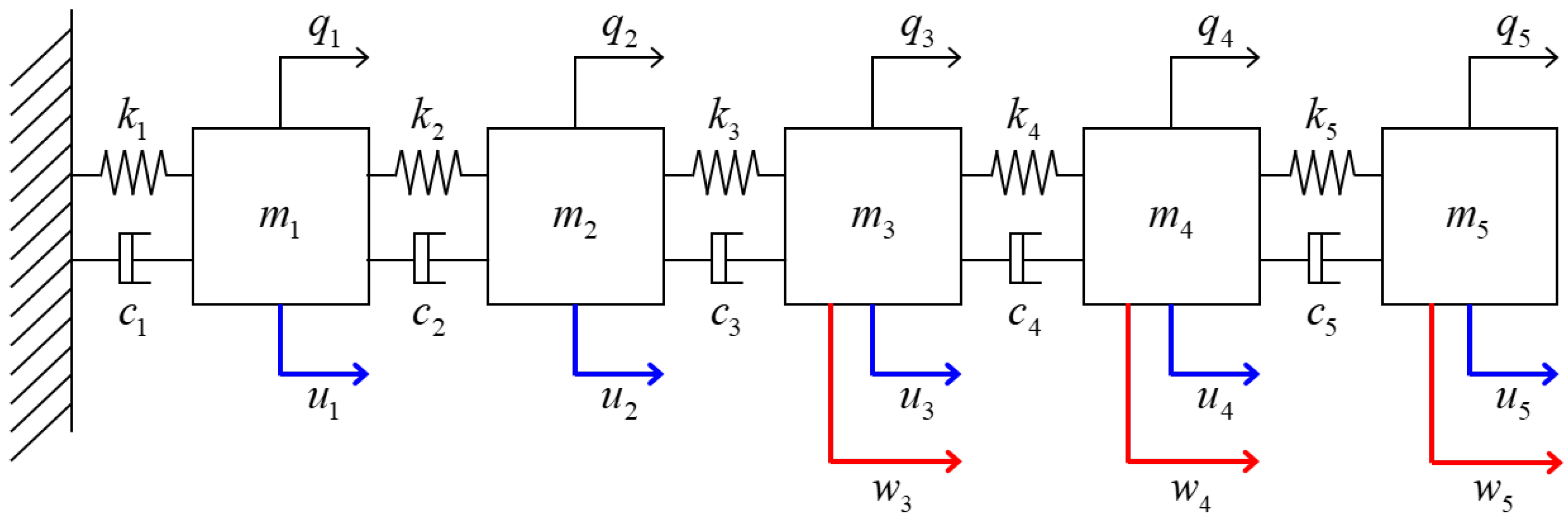
Consider the five-mass spring–damper system illustrated in Figure 2. The system consists of five identical masses connected in series by linear springs and viscous dampers, where the left end is fixed and the right end is free. Let
denote the displacement vector. The second-order dynamics are described by
where denotes the ith standard basis vector and represents an actuator acting on the ith mass. The disturbance distribution matrix in the second-order model is defined as
so that disturbances may act on the third, fourth, and fifth masses.
Figure 2.
Five-mass spring–damper system with candidate actuator locations and disturbance inputs , , and acting on the third, fourth, and fifth masses, respectively. The blue arrows indicate the candidate control inputs, whereas the red arrows indicate the disturbance inputs.
The normalized model parameters are selected as , , and the damping matrix is chosen to be proportional to the stiffness matrix with a proportionality coefficient of . Accordingly,
By defining the state vector as
the system can be written in the state-space form of (1), where
Thus, five candidate actuator configurations are considered as
corresponding to an actuator located at each of the five masses. The resulting state matrix A is Hurwitz, and the pair is controllable for all five candidate actuator locations.
The disturbance vector is given by
and its covariance matrix characterizes the disturbance intensities and correlations associated with the three admissible disturbance locations. The disturbance matrix can equivalently be written as
where denotes the state-space disturbance direction corresponding to a force acting on the jth mass. In the following subsections, the same system and actuator candidates are used to investigate actuator placement under two different forms of covariance uncertainty: total additional disturbance-power uncertainty and spatial disturbance-power uncertainty.
To assess the numerical conditioning of the five candidate configurations, the minimum eigenvalue and the 2-norm condition number of each steady-state controllability Gramian were computed, together with the relative Lyapunov residuals defined in (42). The results are reported in Table 2.
Table 2.
Numerical conditioning of the controllability Gramians and relative Lyapunov residuals.
All five Gramians are numerically positive definite, with minimum eigenvalues between and . Their condition numbers range from to , with having the smallest eigenvalue and the largest condition number. Thus, is relatively more sensitive to numerical perturbations in inverse-related computations, although its condition number alone does not establish that the calculation is unreliable. For every configuration, both normalized Lyapunov residuals are below , indicating that the computed Gramians and auxiliary matrices satisfy their respective equations with small relative residuals despite differences in conditioning. Furthermore, replacing explicit inversion with linear system solves did not alter the robust DoDR rankings for either uncertainty model. These results support the numerical consistency of the present example.
The Gramian and robust DoDR calculations were performed in MATLAB R2025a using double-precision arithmetic. For each actuator configuration, the Lyapunov equations in (8) and (18) were solved using the built-in lyap function, and inverse-related computations were performed through linear system solves. The robust DoDR values were then evaluated using (31) and (36) for the corresponding uncertainty models, following Algorithm 1.
4.2. Actuator Placement Under Total Additional Disturbance-Power Uncertainty
We first consider the total additional disturbance-power uncertainty model introduced in (29). The nominal disturbance is assumed to act exclusively on the fifth mass with unit intensity. Accordingly, the nominal covariance matrix is chosen as
For this nominal covariance, the actuator located at the fifth mass provides the smallest nominal DoDR among the five candidate configurations, i.e., .
As defined in (30), the additional covariance uncertainty is described by
where specifies the upper bound on the total additional disturbance power. Using the closed-form expression derived in (31), the robust DoDR for each candidate actuator configuration is evaluated as
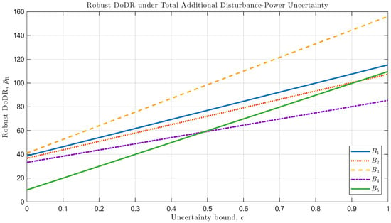
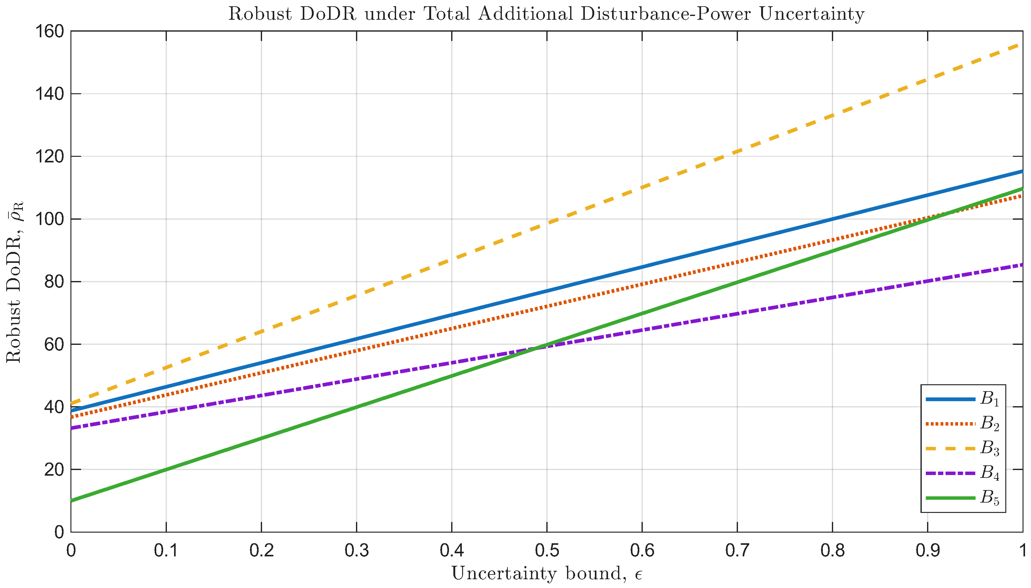
Figure 3 shows the robust DoDR of the five candidate actuator configurations as the uncertainty bound varies from 0 to 1. At , the robust DoDR reduces to the nominal DoDR, and is the optimal actuator configuration. However, the robust DoDR associated with increases more rapidly with than that associated with . According to (31), the slope of each curve is determined by . Thus, although provides the best disturbance-rejection controllability under the nominal covariance, it exhibits greater sensitivity to additional disturbance-power uncertainty than .
Figure 3.
Robust DoDR of the five candidate actuator configurations as a function of the total additional disturbance-power uncertainty bound .
Table 3 summarizes the robust DoDR values at two representative uncertainty levels. For , remains the optimal actuator configuration, with . In contrast, for , the minimum robust DoDR is obtained with , for which . Hence, the actuator configuration that is optimal for the nominal disturbance statistics does not necessarily remain optimal when additional covariance uncertainty is taken into account.
Table 3.
Robust DoDR values for representative levels of total additional disturbance-power uncertainty. Bold values indicate the minimum robust DoDR at each uncertainty level.
From the closed-form expression in (31), the uncertainty level at which the robust DoDR values of and become equal is obtained as
Consequently, is the optimal actuator configuration for , whereas becomes optimal for . At , both and attain the same minimum robust DoDR and are, therefore, equally optimal. This result illustrates the trade-off between nominal disturbance-rejection performance and sensitivity to covariance uncertainty and demonstrates that consideration of disturbance covariance uncertainty can change the preferred actuator placement.
4.3. Actuator Placement Under Spatial Disturbance-Power Uncertainty
We next consider the spatial disturbance-power uncertainty model in which the total disturbance power is known, whereas its spatial distribution among the admissible disturbance locations is unknown. As defined in (35), the corresponding covariance uncertainty set is described by
For the five-mass system considered here, the three disturbance channels correspond to the third, fourth, and fifth masses. The total disturbance power is normalized to , and thus (60) becomes
According to the closed-form result in (36), the robust DoDR for each candidate actuator configuration is evaluated as
where the factor is omitted because . Here, the indices 1, 2, and 3 of correspond to the disturbance directions , , and , respectively. The resulting robust DoDR values for the five candidate actuator configurations are summarized in Table 4.
Table 4.
Robust DoDR values under spatial disturbance-power uncertainty. The minimum robust DoDR is highlighted in bold.
Applying the controller-independent Gramian-screening criterion used in [21] to the present five-mass model selects , which has the largest in Table 2. In contrast, the robust DoDR criterion selects , as shown in Table 4. This same-model comparison illustrates the difference between generic controllability enhancement and covariance-aware disturbance-rejection placement.
To examine the effect of considering uncertainty in disturbance location, the stationary LQR performance of all five configurations is first evaluated, followed by time-domain simulations of representative configurations. This LQR evaluation does not aim to establish a general equivalence between robust DoDR and LQR-optimal placement. The DoDR is a controller-independent, preview-based criterion, and its actuator ranking need not coincide with that based on a specific closed-loop performance objective. When a particular controller and its performance objective are specified in advance, directly evaluating that objective may be more appropriate for actuator placement. Nevertheless, DoDR can guide actuator placement before a controller is selected. The LQR evaluation, therefore, serves to examine whether the relative disturbance-rejection characteristics indicated by DoDR are reflected in closed-loop responses under a comparable control-power constraint.
For each of the five candidate actuator configurations, a continuous-time LQR controller is designed as
where is obtained by minimizing the standard quadratic performance index
The cost in (64) defines the nominal infinite-horizon LQR regulator design problem; it is not interpreted as a finite expected accumulated cost under persistent stochastic disturbances. The stochastic closed-loop performance is instead characterized by the stationary mean-square measures introduced below. The state weighting matrix is fixed as , whereas the scalar input weighting is adjusted separately for each actuator configuration as described below.
For a stable closed-loop system and a unit-power white-noise disturbance acting through , the stationary state covariance is obtained from the continuous-time algebraic Lyapunov equation [29]
Here, , , and denote the disturbance directions associated with disturbances acting on masses 3, 4, and 5, respectively. The corresponding steady-state mean-square state response and control input are evaluated as
To compare all five actuator configurations under the same design rule, is numerically adjusted so that the maximum steady-state mean-square control input over the three admissible disturbance locations is identical:
The weights may differ among actuator configurations because they are adjusted to satisfy the same control-power constraint in (68), rather than assigned a common numerical value. Numerically, each is determined using 60 bisection iterations over , with the LQR gain and stationary state covariance recomputed at each iteration.
It is useful to note that disturbances concentrated individually at masses 3, 4, and 5 are sufficient to determine the worst-case steady-state mean-square performance over the entire spatial uncertainty set. For a covariance matrix , the stationary closed-loop covariance satisfies
Since the Lyapunov equation in (69) is linear with respect to the covariance matrix S, and
the corresponding state covariance can be written as
Consequently, the state and control performance measures satisfy
Because and , the quantities in (72) and (73) are convex combinations of the corresponding performances for disturbances concentrated individually at masses 3, 4, and 5. Therefore, their maximum values over are attained for at least one of these three individual disturbance cases. This allows the worst-case steady-state mean-square performance over the spatial uncertainty set to be evaluated by considering the three disturbance locations separately.
Table 5 compares the stationary LQR performance of all five configurations with the robust DoDR rankings from Table 4. The configuration-dependent values of result from enforcing the same worst-case mean-square control-input constraint in (68), so the state responses are evaluated under a common control-power budget.
Table 5.
Robust DoDR ranking and stationary LQR performance under equal worst-case mean-square control input. The minimum worst-case LQR state response is highlighted in bold.
Although the robust DoDR ranking differs from the ordering of the stationary LQR state responses, both criteria identify as the best candidate. In contrast, applying the original DoDR proposed by Kang et al. [22] with a disturbance assumed to act individually at mass 3, 4, or 5 would select , , or , respectively. Thus, when the disturbance location is uncertain, the conventional DoDR may select a configuration such as or , whose worst-case LQR responses are larger than those of . In particular, the worst-case LQR state response of is approximately lower than that of , the next-best LQR configuration. These results illustrate the potential benefit of accounting for disturbance-location uncertainty in actuator placement, although the robust DoDR does not necessarily reproduce the complete LQR performance ranking.
The closed-loop simulations are performed from to with the initial condition and a fixed integration step of . The continuous-time dynamics are numerically integrated using the fourth-order Runge–Kutta method. Unit-intensity Gaussian white noise is approximated by piecewise-constant independent Gaussian samples with variance , where is the integration step. To reduce the influence of the initial transient, the time-averaged squared state norm and squared control input used in the simulation results are evaluated over . For reproducibility, the MATLAB random number generator is initialized with seed 1 for the representative realization and with seed r for the rth Monte Carlo realization, where . Within each realization, the same disturbance sequences are used for all actuator configurations.
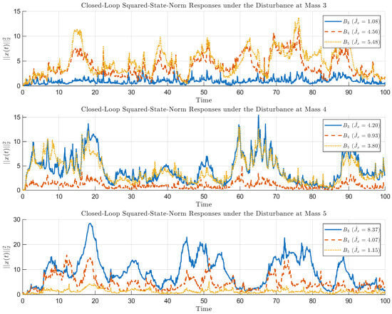
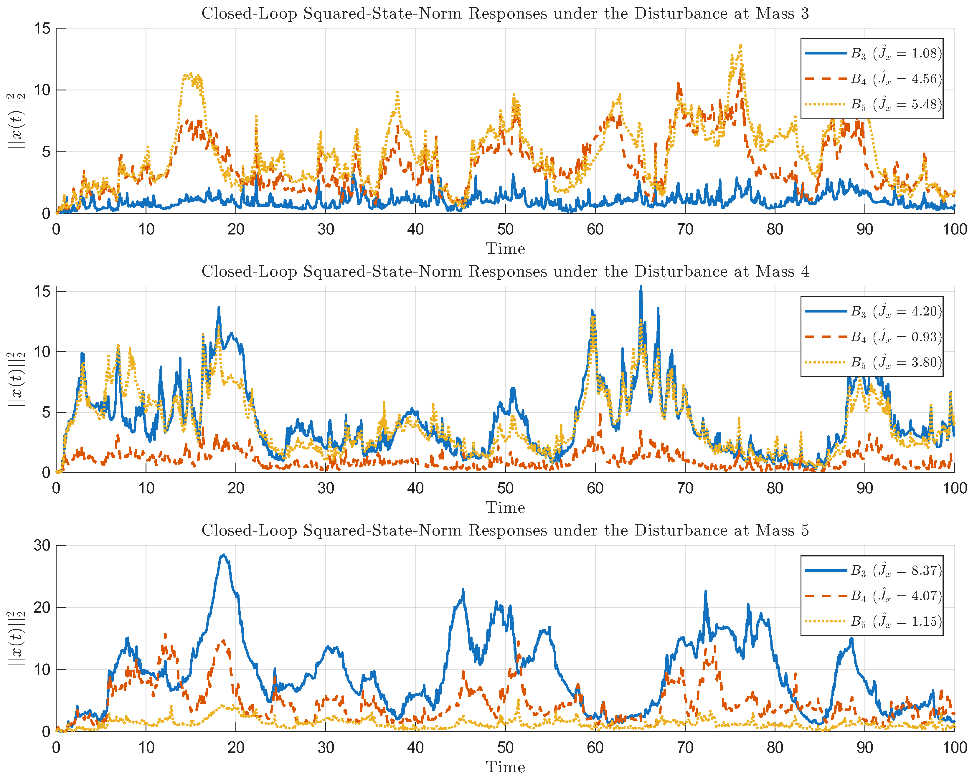
Figure 4 shows the squared-state-norm responses of , , and for unit-power disturbances acting individually at masses 3, 4, and 5. For each disturbance location, the same disturbance realization is applied to all three actuator configurations. To distinguish the finite-time simulation averages from the stationary mean-square quantities defined in (66) and (67), the time-averaged squared state norm and squared control input are denoted by and , respectively. Configurations and exhibit smaller responses for disturbances at their respective actuator locations, whereas provides a more balanced response across the three disturbance locations.
Figure 4.
Closed-loop squared-state-norm responses of actuator configurations , , and under unit-power disturbances acting individually at masses 3, 4, and 5. The same disturbance realization is applied to all three configurations for each disturbance location. The legends indicate the time-averaged squared state norms, .
The corresponding time-averaged performance values for the representative disturbance realization in Figure 4 are summarized in Table 6. Although (68) equalizes the worst-case stationary mean-square control input of all three configurations, the finite-time sample averages differ from their stationary values because they are obtained from one stochastic realization. The responses of and are smallest for disturbances at masses 3 and 5, respectively, whereas shows relatively moderate responses across the three locations. The corresponding stationary worst-case comparison is given in Table 5.
Table 6.
Time-averaged LQR performance for the representative disturbance realization shown in Figure 4.
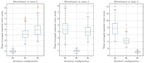
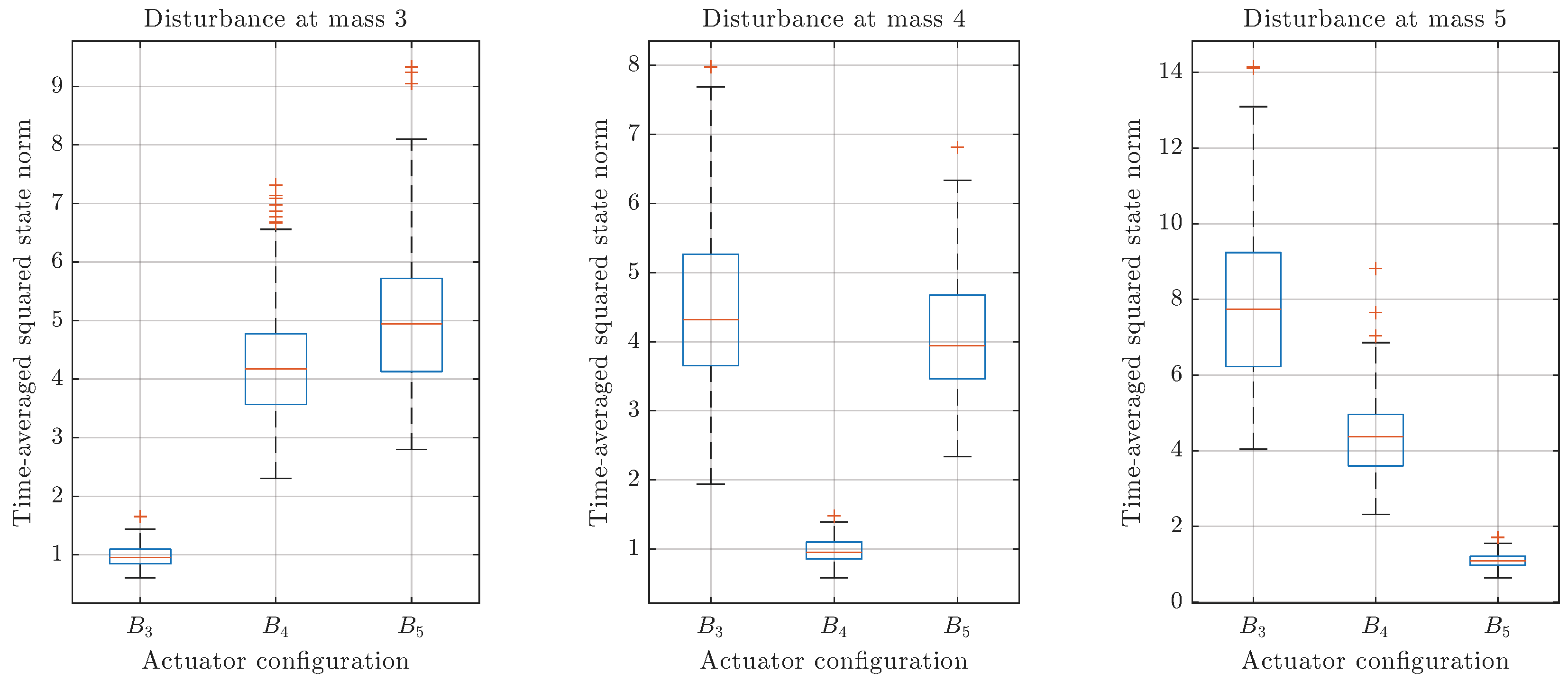
To reduce the dependence of the time-domain comparison on a particular stochastic disturbance realization, the LQR simulations are repeated for 100 independent disturbance realizations. For each realization and disturbance location, the same disturbance sequence is applied to all three configurations. Figure 5 compares the resulting distributions of the time-averaged squared state norm for , , and .
Figure 5.
Distributions of the time-averaged squared state norm over 100 independent disturbance realizations for actuator configurations , , and under disturbances acting individually at masses 3, 4, and 5. Blue boxes represent the interquartile range (25th–75th percentiles), with orange lines indicating the medians. Whiskers extend to the most extreme data points within 1.5 times the interquartile range, and orange plus signs indicate outliers.
As shown in Figure 5, the distributions of the time-averaged squared state norm vary with the actuator and disturbance locations. Configurations and exhibit smaller responses for disturbances at masses 3 and 5, respectively, whereas shows relatively moderate responses across the three disturbance locations. The boxplots also illustrate the variability of the responses over different disturbance realizations, which is not apparent from the single realization in Figure 4.
To evaluate the agreement between the simulations and stationary predictions, Table 7 reports the sample mean, standard deviation, and 95% confidence interval of the time-averaged squared state norm from the 100 independent disturbance realizations. The confidence intervals for the Monte Carlo means are computed using Student’s t-distribution with 99 degrees of freedom. The stationary values are obtained independently from (66).
Table 7.
Stationary mean-square state responses and Monte Carlo statistics from 100 disturbance realizations.
Since identical disturbance realizations are used for different actuator configurations, paired differences can be evaluated for each disturbance location. Table 8 reports the mean paired differences in between and , for , together with the 95% confidence-interval half-widths. Positive values indicate a smaller time-averaged squared state norm for .
Table 8.
Paired differences in time-averaged squared state norms (mean ± 95% confidence-interval half-width) for the same disturbance realizations.
As shown in Table 7, the Monte Carlo means are close to the stationary covariance predictions, with all nine stationary values falling within the corresponding 95% confidence intervals. The paired comparisons in Table 8 further confirm that the relative performance of the actuator configurations depends on the disturbance location. In particular, and provide smaller responses than for disturbances at masses 3 and 5, respectively, whereas performs better under the other disturbance locations. Nevertheless, achieves the smallest worst-case state response when evaluated across all three disturbance locations, consistent with the stationary results in Table 5.
5. Conclusions and Future Work
This study developed a controller-independent robust DoDR-based actuator-placement framework under disturbance covariance uncertainty. For asymptotically stable and controllable LTI systems, an auxiliary Lyapunov equation yields a covariance-linear representation of the steady-state DoDR, , allowing the worst-case criterion to be characterized by the support function of the covariance uncertainty set. Based on this representation, closed-form robust DoDR expressions were derived for total additional disturbance-power uncertainty and spatial disturbance-power uncertainty, involving the largest eigenvalue and the largest diagonal entry of , respectively. These results extend the original DoDR-based placement criterion beyond prescribed disturbance statistics without requiring feedback-controller design.
Numerical results for a five-mass spring–damper system demonstrated the effect of covariance uncertainty on actuator selection. Under total additional disturbance-power uncertainty, the optimal configuration changed from to when the uncertainty bound exceeded , with both configurations equally optimal at the threshold. Under spatial disturbance-power uncertainty, the robust DoDR selected among five candidates. With the same worst-case mean-square control-input constraint, also achieved the smallest worst-case stationary LQR mean-square state response (, versus for ), corresponding to a reduction of approximately . The 100-realization Monte Carlo results were consistent with the stationary covariance predictions, providing an additional closed-loop illustration of the proposed actuator-placement criterion.
The framework assumes asymptotically stable and controllable LTI systems with predefined actuator configurations. The support-function characterization applies to nonempty compact convex covariance uncertainty sets, although its evaluation may require numerical optimization beyond the two uncertainty models with closed-form solutions considered here. Future work will examine more general covariance uncertainty, unstable or marginally stable dynamics, and broader actuator-allocation problems. Engineering applications, including building vibration control under seismic excitation [34], will require suitable dynamical and disturbance covariance models and further validation through higher-fidelity simulations and experiments.
Author Contributions
Conceptualization, H.L.; methodology, H.L.; software, H.L.; validation, H.L. and D.L.; formal analysis, H.L.; writing—original draft preparation, H.L.; writing—review and editing, H.L. and D.L.; visualization, H.L.; funding acquisition, H.L. All authors have read and agreed to the published version of the manuscript.
Funding
This research was supported by the ANCHOR program through the Chungcheongnam-do ANCHOR Center, funded by the Ministry of Education (MOE) and Chungcheongnam-do, Republic of Korea (2026-ANCHOR-12-003). This research was also supported by the Glocal University 30 Project funded by the Ministry of Education (Republic of Korea). In addition, this work was supported by a National Research Foundation of Korea (NRF) grant funded by the Korean government (Ministry of Science and ICT, MSIT) (RS-2026-25600375). Furthermore, this research was supported by the Basic Science Research Program through the NRF, funded by the Ministry of Education (RS-2026-25576586).
Data Availability Statement
The original contributions presented in this study are included in the article. Further inquiries can be directed to the corresponding author.
Conflicts of Interest
The authors declare no conflicts of interest.
References
- Hughes, P.; Skelton, R. Controllability and observability of linear matrix-second-order systems. J. Appl. Mech. 1980, 47, 415–420. [Google Scholar] [CrossRef] [Scilit]
- Hamdan, A.; Nayfeh, A. Measures of modal controllability and observability for first- and second-order linear systems. J. Guid. Control Dyn. 1989, 12, 421–428. [Google Scholar] [CrossRef] [Scilit] [PubMed]
- Tarokh, M. Measures for controllability, observability and fixed modes. IEEE Trans. Autom. Control 1992, 37, 1268–1273. [Google Scholar] [CrossRef] [Scilit]
- Viswanathan, C.; Longman, R.; Likins, P. A degree of controllability definition: Fundamental concepts and application to modal systems. J. Guid. Control Dyn. 1984, 7, 222–230. [Google Scholar] [CrossRef] [Scilit] [PubMed]
- Müller, P.; Weber, H. Analysis and optimization of certain qualities of controllability and observability for linear dynamical systems. Automatica 1972, 8, 237–246. [Google Scholar] [CrossRef] [Scilit]
- Marx, B.; Koenig, D.; Georges, D. Optimal sensor and actuator location for descriptor systems using generalized gramians and balanced realizations. In Proceedings of the 2004 American Control Conference, Boston, MA, USA, 30 June–2 July 2004; Volume 3, pp. 2729–2734. [Google Scholar] [CrossRef] [Scilit]
- Singh, A.K.; Hahn, J. Determining optimal sensor locations for state and parameter estimation for stable nonlinear systems. Ind. Eng. Chem. Res. 2005, 44, 5645–5659. [Google Scholar] [CrossRef] [Scilit]
- Zhao, S.; Pasqualetti, F. Networks with diagonal controllability Gramian: Analysis, graphical conditions, and design algorithms. Automatica 2019, 102, 10–18. [Google Scholar] [CrossRef] [Scilit]
- Babazadeh, M. Gramian-based vulnerability analysis of dynamic networks. IET Control Theory Appl. 2022, 16, 625–637. [Google Scholar] [CrossRef] [Scilit]
- Hać, A.; Liu, L. Sensor and actuator location in motion control of flexible structures. J. Sound Vib. 1993, 167, 239–261. [Google Scholar] [CrossRef] [Scilit]
- Roh, H.S.; Park, Y. Actuator and exciter placement for flexible structures. J. Guid. Control Dyn. 1997, 20, 850–856. [Google Scholar] [CrossRef] [Scilit] [PubMed]
- Shaker, H.R.; Tahavori, M. Optimal sensor and actuator location for unstable systems. J. Vib. Control 2013, 19, 1915–1920. [Google Scholar] [CrossRef] [Scilit]
- Alves da Silveira, O.A.; Ono Fonseca, J.S.; Santos, I.F. Actuator topology design using the controllability Gramian. Struct. Multidiscip. Optim. 2015, 51, 145–157. [Google Scholar] [CrossRef] [Scilit]
- Brand, Z.; Cole, M.O.T. Controllability and actuator placement optimization for active damping of a thin rotating ring with piezo-patch transducers. J. Sound Vib. 2020, 472, 115172. [Google Scholar] [CrossRef] [Scilit]
- Brand, Z.; Cole, M.O.T. Mini-max optimization of actuator/sensor placement for flexural vibration control of a rotating thin-walled cylinder over a range of speeds. J. Sound Vib. 2021, 506, 116105. [Google Scholar] [CrossRef] [Scilit]
- Lee, H.; Park, Y. Degree of controllability for linear unstable systems. J. Vib. Control 2016, 22, 1928–1934. [Google Scholar] [CrossRef] [Scilit]
- Lee, H. Controllability-based metric for actuator allocation in linear systems with semi-stable modes. J. Frankl. Inst. 2026, 363, 108948. [Google Scholar] [CrossRef] [Scilit]
- Hovd, M.; Skogestad, S. Simple frequency-dependent tools for control system analysis, structure selection and design. Automatica 1992, 28, 989–996. [Google Scholar] [CrossRef] [Scilit]
- Cao, Y.; Rossiter, D.; Owens, D. Input selection for disturbance rejection under manipulated variable constraints. Comput. Chem. Eng. 1997, 21, S403–S408. [Google Scholar] [CrossRef] [Scilit]
- Mirza, M.A.; Van Niekerk, J.L. Optimal actuator placement for active vibration control with known disturbances. J. Vib. Control 1999, 5, 709–724. [Google Scholar] [CrossRef] [Scilit]
- Demetriou, M.A.; Moghani, T. Robust actuator placement in flexible plates subject to worst-case spatial distribution of disturbances. In Proceedings of the 2004 American Control Conference, Boston, MA, USA, 30 June–2 July 2004; Volume 4, pp. 3550–3555. [Google Scholar] [CrossRef] [Scilit]
- Kang, O.; Park, Y.; Park, Y.S.; Suh, M. New measure representing degree of controllability for disturbance rejection. J. Guid. Control Dyn. 2009, 32, 1658–1661. [Google Scholar] [CrossRef] [Scilit]
- Xia, Y.; Yin, M.; Cai, C.; Zhang, B.; Zou, Y. A new measure of the degree of controllability for linear system with external disturbance and its application to wind turbines. J. Vib. Control 2018, 24, 739–759. [Google Scholar] [CrossRef] [Scilit]
- Xia, Y.; Yin, M.; Li, R.; Liu, D.; Zou, Y. Integrated structure and maximum power point tracking control design for wind turbines based on degree of controllability. J. Vib. Control 2019, 25, 397–407. [Google Scholar] [CrossRef] [Scilit]
- Xia, Y.; Li, R.; Yin, M.; Zou, Y. A quantitative measure of the degree of output controllability for output regulation control systems: Concept, approach, and applications. J. Vib. Control 2022, 28, 2803–2815. [Google Scholar] [CrossRef] [Scilit]
- Lee, H.; Park, J. Quantitative controllability metric for disturbance rejection in linear unstable systems. Mathematics 2025, 13, 6. [Google Scholar] [CrossRef] [Scilit]
- Lee, H. Controllability measure for disturbance rejection capabilities of control systems with undamped flexible structures. J. Frankl. Inst. 2024, 361, 107320. [Google Scholar] [CrossRef] [Scilit]
- Lee, H.; Park, J. Steady-state disturbance-rejection controllability for LTI systems with rigid-body mode. Actuators 2025, 14, 589. [Google Scholar] [CrossRef] [Scilit]
- Kwakernaak, H.; Sivan, R. Linear Optimal Control Systems; Wiley-Interscience: New York, NY, USA, 1972. [Google Scholar]
- Boyd, S.; Vandenberghe, L. Convex Optimization; Cambridge University Press: Cambridge, UK, 2004. [Google Scholar] [CrossRef] [Scilit]
- Bertsekas, D.P. Convex Optimization Theory; Athena Scientific: Belmont, MA, USA, 2009. [Google Scholar]
- Simoncini, V. Computational methods for linear matrix equations. SIAM Rev. 2016, 58, 377–441. [Google Scholar] [CrossRef] [Scilit]
- Higham, N.J. Accuracy and Stability of Numerical Algorithms, 2nd ed.; Society for Industrial and Applied Mathematics: Philadelphia, PA, USA, 2002. [Google Scholar] [CrossRef] [Scilit]
- Humaidi, A.J.; Sadiq, M.E.; Abdulkareem, A.I.; Ibraheem, I.K.; Azar, A.T. Adaptive backstepping sliding mode control design for vibration suppression of earth-quaked building supported by magneto-rheological damper. J. Low Freq. Noise Vib. Act. Control 2022, 41, 768–783. [Google Scholar] [CrossRef] [Scilit]



Disclaimer/Publisher’s Note: The statements, opinions and data contained in all publications are solely those of the individual author(s) and contributor(s) and not of MDPI and/or the editor(s). MDPI and/or the editor(s) disclaim responsibility for any injury to people or property resulting from any ideas, methods, instructions or products referred to in the content. |
© 2026 by the authors. Licensee MDPI, Basel, Switzerland. This article is an open access article distributed under the terms and conditions of the Creative Commons Attribution (CC BY) license.