


Abstract
Second-price sealed-bid auctions with collusion are well studied, but the role of bidders’ risk aversion remains unclear. We study a two-bidder auction with heterogeneous constant relative risk aversion under the variable-bribe and fixed-bribe mechanisms, characterize the corresponding collusive equilibria, and examine effects on collusion and the seller’s expected revenue. Under the variable-bribe mechanism, we obtain an equilibrium in which lower proposer values separate and higher values pool. Greater proposer risk aversion increases the bribe, the responder’s acceptance cutoff, the probability of successful collusion, and the probability of misallocation, while reducing the seller’s expected revenue. Responder risk aversion does not affect the equilibrium. Under the fixed-bribe mechanism, primitive sufficient conditions establish a regular interior cutoff equilibrium. Within this regular interior equilibrium class, greater responder risk aversion raises the responder’s acceptance cutoff and the probability of misallocation, but lowers the proposer’s offer cutoff and the seller’s expected revenue. Greater proposer risk aversion lowers both the proposer’s offer cutoff and the responder’s acceptance cutoff, while its effects on the probability of successful collusion and the seller’s expected revenue can be positive or negative. Finally, we briefly discuss four extensions: variable-bribe collusive equilibria with positive initial wealth or a reserve price, and fixed-bribe collusive equilibria with general concave utility or an endogenously determined amount.
Keywords:
second-price sealed-bid auction; bribery; collusion; heterogeneous risk aversion; constant relative risk aversion; allocative efficiency; seller revenue MSC:
91B26; 91A27; 91B16
1. Introduction and Literature Review
1.1. Introduction
Second-price sealed-bid auctions are among the most fundamental mechanisms in auction theory. Vickrey’s classic analysis establishes truthful bidding [1], and its state-by-state dominance argument also preserves truthful bidding under strictly increasing utility. Bolotnyy and Vasserman [2] find infrastructure procurement bids consistent with firms limiting quantity-risk exposure, providing an empirical motivation for risk-averse preferences. When bidders can collude, internal transfer payments may increase their payoffs at the seller’s expense. Decarolis, Goldmanis, and Penta [3] show how common-agency coordination of competing advertisers’ bids for multiple positions can lower revenue, a related concern for bilateral agreements. Existing studies examine arrangements that include bidding rings and direct bribery between bidders [4,5,6,7]. Eső and Schummer [4], in particular, study bilateral collusion in a second-price sealed-bid auction in which one bidder offers the other a fixed or variable bribe to submit a zero bid. Eső and Schummer’s analysis assumes risk neutrality. We extend Eső and Schummer’s [4] analysis of bilateral collusion to risk-averse bidders and further allow the two bidders to differ in their degrees of risk aversion. Because the proposer and responder occupy different strategic roles in bilateral collusion, heterogeneous risk aversion allows us to identify more fully how each bidder’s risk aversion affects the collusive equilibrium. We assume that the two roles have different constant relative risk aversion (CRRA) preferences. The proposer offers a bribe in exchange for the responder’s zero bid; acceptance gives the proposer the object at a zero auction price, while rejection leads to truthful bidding. The two mechanisms differ in the proposer’s choice: under variable bribes, it chooses the amount according to its own valuation, whereas under fixed bribes, the amount is specified in advance and it chooses only whether to offer it.
The main contribution is to identify how heterogeneous risk preferences affect collusion through the proposer’s offer decision and the responder’s acceptance decision, with qualitatively different effects across the two bribery mechanisms. More specifically, the paper makes four contributions. First, it extends the literature on collusion in second-price sealed-bid auctions [4,5,6] by analyzing the effects of bidders’ risk aversion on the collusive equilibrium, allocative efficiency, and the seller’s expected revenue. Second, it extends the two-bidder pre-auction bribery model of Eső and Schummer [4] from risk-neutral to risk-averse bidders, building on Llorente-Saguer and Zultan’s [8] observation that risk aversion changes the bribery schedule. Under variable bribes, although the schedule retains the Eső–Schummer form under a transformed distribution, we further introduce positive initial wealth to examine the potential equivalence arising from utility homogeneity and assess the robustness of our findings on the effects of risk aversion on the collusive equilibrium. Third, by allowing heterogeneous risk aversion, we identify separately how the proposer’s and responder’s risk aversion affects the collusive equilibrium. For fixed bribes, these comparisons hold within the regular interior cutoff equilibrium under the stated primitive sufficient conditions. Fourth, we extend the analysis of collusive equilibria in second-price sealed-bid auctions to reserve prices and endogenously determined fixed bribes.
The remainder of the paper is organized as follows. Section 1.2 reviews the related literature. Section 2 presents the model. Section 3 and Section 4 analyze variable and fixed bribes, respectively. Section 5 examines the seller’s expected revenue under the two mechanisms. Section 6 develops the extensions. Section 7 concludes. Appendix A contains all proofs.
1.2. Literature Review
The closest model is the bilateral pre-auction bribery game of Eső and Schummer [4]. A variable offer reveals lower proposer values, with higher values pooling once acceptance is certain, whereas a fixed offer identifies only an offering pool. Both protocols can generate inefficient allocation, but the different information available at the acceptance stage changes the responder’s decision. This bilateral offer differs from the internal allocation and transfer mechanisms studied by Graham and Marshall [5] for single-object second-price and English rings and McAfee and McMillan [7] for first-price cartels. Meanwhile, without bid control, Marshall and Marx [6] show that a ring can eliminate all internal competition under second-price but not first-price rules. Mailath and Zemsky [9] show that efficient second-price collusion is possible with asymmetric value distributions.
Later bilateral models change the bargaining sequence or available proposals. Rachmilevitch [10] introduces two sequential bribing opportunities and characterizes efficient equilibria under pure strategies and a refinement. Lu, Lu, and Riis [11] allow both an offered bribe and a requested payment, obtaining a robust equilibrium with certain collusion. With random outside competition and difficulties in verifying compliance, Chen and Tauman [12] use a price-dependent side-payment mechanism to address incentives to use shill bidders. Rachmilevitch’s first-price bribery analysis [13] provides an auction-rule comparison, with its corrigendum clarifying sufficient conditions for zero-bribe equilibrium existence. Deng [14] studies pre-auction acquisitions in single-object procurement, another way of reducing competition before bidding. These studies connect the form of an agreement to the gains from collusion and incentives to disclose private information.
The value environment also matters. Troyan [15] studies interdependent values and affiliated signals. Acceptance can lead the proposer to revise its estimate of the object’s value, creating a briber’s curse, particularly with outside competition. In our independent-private-values environment, an offer does not change either bidder’s own valuation. Belief updating instead affects the responder’s distribution of auction surplus after rejection.
Experiments connect these information and transfer channels to behavior. Llorente-Saguer and Zultan [8] study bribery in first- and second-price auctions; failed negotiations can distort subsequent first-price bidding. Agranov and Yariv [16] examine communication and voluntary post-auction transfers, rather than the binding bilateral commitment assumed here. Noussair and Seres [17] find that second-price bidding rings reduce experimental efficiency, connecting collusion to the misallocation examined here. Sujarittanonta and Viriyavipart [18] investigate reserve prices as a deterrent to collusion in first-price auction experiments, finding lower average bribe offers and a lower rate of successful bribes. Hsueh et al. [19] link two-stage Chinese land auctions with secret reserves to patterns consistent with collusion. This motivates attention to reserves, which we examine in a second-price environment. Eső and Schummer’s supplement [20] provides the risk-neutral reserve-price extension of both bribery protocols.
Risk aversion introduces a further distinction between the protocols. Pratt [21] provides the preference comparison underlying our concave-transformation extension. Zhang and Liu [22] study how default affects the revenue consequences of risk aversion with uncertain valuations in second-price auctions. Bos, Gomez-Martinez, and Onderstal [23] examine risk-averse bidding when bidders care about an outside observer’s assessment of their values. These studies connect risk effects to the uncertainty and information entering bidders’ payoffs. Truthful second-price bidding follows from the classical state-by-state dominance argument [1], which strictly increasing utility preserves. Before bidding, however, a revealing variable offer makes the responder’s rejection payoff known, whereas a fixed offer leaves a lottery over proposer values. Because the upper pooled variable offer is also accepted by every responder through a statewise payoff comparison, responder risk aversion affects the fixed-bribe acceptance decision but not the variable-bribe equilibrium. We examine how these information differences generate role-specific risk effects, including the respective extensions to positive wealth, a reserve price, and general concavity.
2. Model
A seller allocates one indivisible object through a second-price sealed-bid auction. There are two bidders. Bidder P is the potential proposer and bidder R is the potential responder. Their values are independent and identically distributed and satisfy
where F(0) = 0, , F is continuously differentiable, and f > 0 on . Each bidder observes only its own value. Their utilities over payoffs y are
The power utilities are defined over nonnegative monetary surplus from the auction and the agreement. The proposer’s and responder’s coefficients of relative risk aversion are 1 − a and 1 − d, respectively, and belong to [0,1). These parameters describe curvature over gains without initial wealth. Section 6 examines CRRA utility over positive initial wealth and separate general-utility extensions.
A lower exponent represents greater relative risk aversion. If no agreement is reached, both bidders enter the auction and bid truthfully. Truthful bidding remains weakly dominant under every strictly increasing utility, so continuation monetary payoffs are (v − x)+ for the proposer and (x − v)+ for the responder, and the seller receives min{v, x}.
The pre-auction stage follows the two bribery mechanisms in Eső and Schummer [4]. Under the variable-bribe mechanism, a proposer of type v chooses a bribe b ∈ [0,v]. Under the fixed-bribe mechanism, a bribe is specified. A proposer with v ≥ β chooses whether to make the fixed-bribe offer. A proposer with v < β does not make the offer. The responder observes the offer and its own value, then accepts or rejects. Acceptance commits the responder to submit a zero bid. The proposer receives the object and pays the bribe, and the seller receives no auction payment. Rejection leads to the truthful second-price auction. Strategies and beliefs form a perfect Bayesian equilibrium (PBE).
Following the exogenously fixed-transfer formulation of Eső and Schummer [4], under the fixed-bribe protocol, β is a publicly known transfer specified by a pre-existing agreement opportunity before private values are realized. Economically, this can represent a standardized payment stipulated by a prior arrangement between the bidders. The baseline takes that amount as given: neither bidder chooses it within the game, and after observing its valuation, the proposer decides only whether to use the opportunity. Acceptance is binding, committing the proposer to the specified payment and the responder to a zero bid, with no subsequent renegotiation. Thus, the amount is fixed in advance, but payment occurs only if an offer is made and accepted. Section 6.4 instead assigns the public, pre-valuation choice of the amount to the proposer.
For the continuous equilibrium with an upper pooling region studied below, assume that F is log-concave and, for every , satisfies the elasticity condition
Log-concavity makes the equilibrium type map monotone. The elasticity bound guarantees global incentive compatibility (IC) under constant relative risk aversion. It is automatic at a = 1, and power cumulative distribution functions with k ≥ 1 satisfy all these conditions. The fixed-bribe analysis uses the regular interior cutoff equilibria defined in Section 4.
3. Variable Bribe
For a separating offer that reveals proposer value v and specifies bribe b, a responder of value x receives b upon acceptance and the known amount (x − v)+ upon rejection. The responder therefore accepts exactly when x ≤ v + b. Write this acceptance cutoff as q = v + b and the proposer’s surplus after acceptance as g = v − b. For , the separating candidate can be parameterized as
Here, we parameterize v, b, and g by the responder’s acceptance cutoff q.
Remark 1.
The endogenous acceptance cutoff q parameterizes the proposer’s value, bribe, and surplus. Conditional on the proposer’s value v, the relevant objects are the equilibrium bribe b(v), the proposer’s monetary payoff after successful collusion g(v), and the responder’s acceptance cutoff q(v). Appendix A establishes a one-to-one correspondence between v and q on the separating region, so the objects in Equation (1) can equivalently be expressed as functions of v.
Set g(0) = v(0) = b(0) = 0. Log-concavity implies that v is strictly increasing. Let q = v−1 on its range, with q(0) = 0, and set
The cutoff c is the proposer value at which the acceptance set reaches the top of the responder’s value support. Our first proposition gives the proposer’s separating offer strategy with an upper pooling region under the variable-bribe mechanism.
Proposition 1.
Under the variable-bribe mechanism in the model of Section 2, a perfect Bayesian equilibrium is given by
An offer specifying the bribe b(q) below reveals type v(q) and is accepted iff x ≤ q. The offer specifying the bribe is made by all types v ≥ c and is accepted by every responder type. On the separating part, the equilibrium bribe also solves
Proof.
See Appendix A. □
Remark 2.
If F is log-concave and zf(z)/F(z) ≥ 1 on , then, as a ↓ 0,
uniformly on the value support. Moreover, ga(q) → 0 uniformly for , , and .
Proof.
See Appendix A. □
Remark 3.
Log-concavity is sufficient for the continuous construction but is not necessary for the existence of an equilibrium. On [0,1], the non-log-concave distribution F(v) = v exp[0.6(v2 − 1)] supports the same equilibrium for 0.2 < a ≤ 1. A second distribution in Appendix A admits a non-collusive PBE even though the candidate separating type map is nonmonotone.
Proof.
See Appendix A. □
Remark 4.
Because CRRA utility without initial wealth is homogeneous, the separating schedule has a transformed-distribution representation. For a true proposer value v0 and an offer indexed by q ≥ v0, the reduced objective has the same maximizers as F(q)1/a[v0 − b(q)]. The candidate schedule therefore coincides with the Eső–Schummer schedule under Ga = F1/a. To compare risk preferences, however, we hold F fixed; a downward deviation with q < v0 has expected utility
Section 6.1 introduces positive initial wealth and establishes the proposer-risk direction beyond homogeneous utility over auction gains.
We next study how the bidders’ risk aversion and the value distribution affect the equilibrium bribe function and the responder’s acceptance cutoff. Define the acceptance frontier
The reverse hazard rate f/F measures the marginal proportional increase in acceptance probability from raising the cutoff. A higher rate makes an expanded acceptance set more valuable relative to the bribe’s cost, inducing a weakly higher equilibrium bribe and acceptance frontier, as Proposition 2 shows.
Proposition 2.
Consider two distributions F1 and F2 on in Proposition 1. Suppose that, for every ,
Then b1(v) ≥ b2(v) and Q1(v) ≥ Q2(v) for every proposer value.
Proof.
See Appendix A. □
We next examine how each bidder’s risk aversion affects the separating offer strategy with an upper pooling region. To simplify notation, objects used in the comparative statics for proposer risk aversion carry a subscript a. For example, we rewrite b(v) as ba(v). The collusive agreement converts an uncertain monetary payoff without collusion into a certain monetary payoff under successful collusion. The proposer offers a larger bribe to obtain a higher probability of acceptance. A more risk-averse proposer therefore raises the bribe to reduce uncertainty, which also raises the responder’s acceptance cutoff.
Proposition 3.
Let 0 < a1 < a2 ≤ 1. For every v > 0,
Proof.
See Appendix A. □
Remark 5.
b(v), Q(v) and c are independent of d.
Proof.
See Appendix A. □
We next examine allocative efficiency under the variable-bribe mechanism and the distribution of monetary payoffs between the bidders. We define the probability of successful collusion, the probability of misallocation, and the expected valuation loss respectively as
An accepted offer is inefficient exactly when v < x ≤ Q(v). The responder values the object more, but the responder’s zero bid gives the object to the proposer.
Remark 6.
The equilibrium in Proposition 1 is inefficient with positive probability, and
Moreover, IV(a) and WV(a) are strictly decreasing with a but independent of d.
Proof.
See Appendix A. □
Finally, let and denote the bidders’ ex ante expected monetary payoffs. Our seventh remark shows that greater proposer risk aversion raises the bribe, shifting expected monetary payoff from the proposer to the responder even as successful collusion becomes more frequent.
Remark 7.
strictly increases with a, while strictly decreases with a.
Proof.
See Appendix A. □
4. Fixed Bribes
Under the fixed-bribe mechanism, when the proposer offers the bribe β, the responder learns only that the proposer belongs to the offering pool. Consider cutoff strategies in which the proposer offers iff v ≥ B and the responder accepts iff x ≤ A, with . Bayes’ rule gives the posterior
For later use, define
Here, N(z) is the proposer’s expected utility from entering the auction without an offer, and K(A, B)/[1 − F(B)] is the responder’s expected utility from rejection conditional on observing an offer. At the proposer cutoff, acceptance yields monetary surplus B − β, while rejection yields zero because B < A. The responder at its cutoff instead compares the fixed bribe with a lottery over (A − V)+ under the offer posterior. These two comparisons give the marginal indifference conditions
Equation (3) therefore determines the proposer’s offer cutoff and the responder’s acceptance cutoff jointly.
These indifference conditions identify marginal types; a single-crossing condition ensures that they also describe the offer decisions of the other proposer types. For β < v ≤ A, define
This is the maximum fixed bribe that a high-value proposer is willing to pay for the responder’s zero-bid commitment. We call (B, A) regular when Equation (3) holds, ρ(v; β) > F(A) below B and ρ(v; β) ≤ F(A) from B to A, p(v; A) ≥ β above A, and
The slope inequality makes the proposer incentive cross from no offer to offer at B. The high-type condition is satisfied, for example, when E[X|X ≤ A] ≥ β. Existence can be checked by tracing the two cutoff curves. Let AP(B) and AR(B) denote the proposer and responder solutions to Equation (3) for a given B. A closed interval is a regular crossing interval when both curves are defined there, the proposer single-crossing conditions and the slope inequality hold throughout the interval, and
On such an interval, AP is strictly decreasing and AR is strictly increasing.
Our fourth proposition shows that the cutoff system underlying the fixed-bribe equilibrium has a unique solution on a regular crossing interval.
Proposition 4.
If a regular crossing interval exists, Equation (3) has a unique regular interior solution (B, A) on that interval. The strategies
form a perfect Bayesian equilibrium with the posterior stated above.
Proof.
See Appendix A. □
The next two lemmas give conditions on the primitives that ensure the regular crossing interval required by Proposition 4. The first uses a shape restriction on the value distribution, and the second gives a sharper explicit bound under uniform values.
For , define the certainty equivalent of the highest-value responder’s rejection payoff after truncating proposer values at the primitive level 2t:
Let βG(F,d) be the unique solution of HF,d(t) = t which lies in .
Lemma 1.
Suppose f is nondecreasing. If 0 < β < βG(F,d), a regular crossing interval in Proposition 4 exists. The resulting fixed-bribe equilibrium has
and its positive-offer outcome is essentially unique under the maintained protocol.
Proof.
See Appendix A. □
The amount bound ensures that the highest responder has a sufficiently attractive rejection payoff, while the distribution shape controls the proposer’s global offering incentives. The bound can be checked directly as
Lemma 2.
If values are uniform on and
Proposition 4 has a regular interior equilibrium, and the positive-offer outcome is essentially unique. Its cutoffs satisfy
Proof.
See Appendix A. □
In Lemmas 1 and 2, essential uniqueness means that all perfect Bayesian equilibria in which the fixed bribe is offered with positive probability have the same offer and acceptance cutoffs and induce the same allocation and transfers for almost every valuation pair under the joint value distribution. It does not require unique actions at indifferent cutoff types or unique off-path beliefs, and it does not exclude the zero-offer equilibria discussed in Remark 8.
Remark 8.
Put and, for v ≥ β, define
A zero-offer PBE exists precisely when Δ0(v) ≤ 0 for every feasible proposer type. Under the condition in Lemma 1 with a < 1, no such equilibrium exists. Under uniform values with a = 1 in Lemma 2’s region, a non-collusive outcome coexists with the unique positive-offer outcome.
Proof.
See Appendix A. □
We next examine the effects of risk aversion under fixed bribes. Under the conditions of Lemma 1, the responder equation can be written as the certainty equivalent
Our fifth proposition shows that greater responder risk aversion lowers the proposer’s offer cutoff and raises the responder’s acceptance cutoff.
Proposition 5.
Suppose both parameter configurations being compared satisfy the primitive sufficient conditions of Lemma 1 or Lemma 2. In the corresponding equilibria of Proposition 4, greater responder risk aversion, represented by a fall in d with all other primitives held fixed, produces
The offer probability 1 − F(B), conditional acceptance probability F(A), probability of successful collusion
and expected transfer payment between the two bidders βCF all rise.
Proof.
See Appendix A. □
Unlike a revealing variable offer, a fixed offer leaves uncertainty about the proposer’s value. Greater responder risk aversion lowers the certainty equivalent of rejection, expanding the acceptance set and making an offer profitable for lower-value proposer types. Their entry shifts the posterior distribution of proposer values downward, making rejection more attractive and partly offsetting the direct risk effect. The regular cutoff intersection implies that the direct effect dominates: the acceptance cutoff A rises while the offer cutoff B falls.
We next examine how proposer risk aversion affects collusion under the fixed-bribe mechanism. At a fixed B, Equation (3) can be written
Direct inspection shows that the logarithm of the expectation is convex in a. Because the right-hand side exceeds F(B) at an interior equilibrium, it increases with a. Greater proposer risk aversion therefore makes the fixed-bribe offer more attractive. Our sixth proposition further shows that greater proposer risk aversion lowers both the proposer’s offer cutoff and the responder’s acceptance cutoff.
Proposition 6.
Suppose both parameter configurations being compared satisfy the primitive sufficient conditions of Lemma 1 or Lemma 2. In the corresponding equilibria of Proposition 4, greater proposer risk aversion, represented by a fall in a with all other primitives held fixed, produces
Proof.
See Appendix A. □
Greater proposer risk aversion makes the fixed-bribe offer profitable for additional types and lowers the offer cutoff. With the amount fixed, this entry shifts the distribution of proposer values conditional on an offer downward. Rejection consequently becomes more attractive to the responder, which lowers its acceptance cutoff. Successful collusion thus reflects two opposing changes: a larger offering set and a smaller conditional acceptance set. This interaction between proposer risk aversion and the information conveyed by a fixed offer explains why the probability of successful collusion need not increase.
Without an accepted offer, truthful bidding assigns the object to the higher-value bidder. An accepted offer instead assigns it to the proposer, so misallocation occurs exactly on {B ≤ V < X ≤ A}. Thus
Proposition 7 relates misallocation probability and expected valuation loss to the two cutoff movements induced by responder risk aversion.
Proposition 7.
Under the conditions of Lemma 1 or Lemma 2, in the equilibrium of Proposition 4,
- (i)
- IF > 0, WF > 0;
- (ii)
- d1 < d2 ⇒ IF(B(a, d1), A(a, d1)) > IF(B(a, d2), A(a, d2));
- (iii)
- d1 < d2 ⇒ WF(B(a, d1), A(a, d1)) > WF(B(a, d2), A(a, d2)).
Proof.
See Appendix A. □
A lower offer cutoff adds lower-value proposers to the agreement set, while a higher acceptance cutoff adds higher-value responders. Both changes expand the region in which the responder values the object more, increasing misallocation probability and expected valuation loss. Greater responder risk aversion moves both boundaries in these directions. Greater proposer risk aversion instead lowers both cutoffs, so the two boundary changes have opposing effects on misallocation.
5. Effects of Collusion on the Seller’s Expected Revenue
Both the variable-bribe and fixed-bribe mechanisms affect bidder payoffs and allocative efficiency. They can also reduce the seller’s expected revenue. Let
denote expected seller revenue in the truthful no-collusion benchmark. Under the variable-bribe mechanism, a rejected offer implies x > Qa(v) ≥ v, so the responder wins and pays v. Under the fixed-bribe mechanism, an accepted agreement removes the payment min{v, x} from the seller. The seller’s expected revenue under the two mechanisms is therefore
The first expression integrates the proposer’s value, which the responder pays after rejection. The second subtracts the expected auction payment removed by accepted fixed-bribe offers from the no-collusion benchmark.
An accepted agreement replaces the truthful-auction payment with zero, whereas a rejected or absent offer leaves that payment unchanged. Hence either mechanism reduces expected revenue whenever successful collusion has positive probability.
Remark 9.
Under the variable-bribe mechanism, positive-probability successful collusion implies RV(a) < R0. Under the fixed-bribe mechanism, positive-probability successful collusion implies RF(B, A) < R0.
Proof.
See Appendix A. □
Under variable bribes, greater proposer risk aversion expands the acceptance region, replacing a positive auction payment with zero for additional value pairs. Expected revenue therefore falls. Responder risk aversion leaves that region, and hence revenue, unchanged.
Remark 10.
In the collusive equilibrium characterized in Proposition 1, RV(a) is strictly increasing in a but independent of d.
Proof.
See Appendix A. □
For the fixed-bribe mechanism, define the payments at the two moving boundaries by
The first is the expected payment lost when a proposer at B joins the offer pool. The second is the expected payment restored when a responder at A leaves the acceptance set. Differentiating Equation (4) gives
Because greater responder risk aversion lowers the offer cutoff and raises the acceptance cutoff, both boundary movements remove additional auction payments. This yields the revenue reduction in Remark 11, in contrast to responder-risk invariance under variable bribes.
Remark 11.
Under the conditions of Lemma 1 or Lemma 2, in the equilibrium of Proposition 4, RF(B, A) is strictly increasing in d.
Proof.
See Appendix A. □
Finally, we examine how proposer risk aversion affects the seller’s expected revenue under the fixed-bribe mechanism. For proposer risk aversion, define
The first threshold compares the payments lost and restored at the two margins. The second compares the corresponding probability masses. For every interior pair B < A,
Here, Λ denotes the local quantile-response index along the responder cutoff curve. It is evaluated at the current regular interior equilibrium.
Comparing this response index with the two thresholds separates the change in agreement frequency from the change in forgone auction payments. The next proposition gives the resulting local sign decomposition.
Proposition 8.
Under the conditions of Lemma 1 or Lemma 2, in the equilibrium of Proposition 4, an increase in proposer risk aversion produces three strict local regions:
Proof.
See Appendix A. □
In the outer regions, the probability of successful collusion and the seller’s expected revenue move in opposite directions. The middle region instead allows both to rise because revenue losses depend on the payments removed as well as agreement frequency. A marginal increase in proposer risk aversion lowers B, adding agreements with lower-value proposers, but also lowers A, removing agreements with higher-value responders. At these margins, the added agreements remove less revenue per agreement on average than those that disappear. Thus more agreements can be reached while less total revenue is lost. The following two numerical examples illustrate these regions. These examples establish qualitative attainability rather than necessarily large economic effects. The code used to generate the numerical results and Figure 1, Figure 2, Figure 3, Figure 4, Figure 5 and Figure 6 is provided in the Supplementary Materials.
Figure 1.
Seller revenue along the first parameter path.
Figure 2.
Collusion probability along the first parameter path.
Figure 3.
Collusion probability along the second parameter path.
Figure 4.
Seller revenue along the second parameter path.
Figure 5.
Two-dimensional regions for Example 1 (d = 0.20).
Figure 6.
Two-dimensional regions for Example 2 (d = 0.65).
Example 1.
Let values be uniform on [0,1], set d = 0.20 and β = 0.153, and vary a over [0.2,1]. Figure 1 and Figure 2 trace seller revenue and successful collusion, respectively. The revenue response changes sign at a* = 0.696200, where B = 0.159234 and A = 0.895999. A lower exponent means greater proposer risk aversion. Over the full path, seller revenue ranges from 0.06249942 to 0.06254046, a spread of approximately 0.00004104 (0.06562%). The collusion probability ranges from 0.74684820 to 0.75747832, a spread of 1.06301 percentage points (1.42333%).
Example 2.
Let values be uniform on [0,1], set d = 0.65 and β = 0.094, and vary a over [0.2,1]. The corresponding collusion-probability response changes sign. Figure 3 and Figure 4 report the probability and revenue paths, respectively. Over the full path, the collusion probability ranges from 0.54058575 to 0.54060844, a spread of approximately 0.00226953 percentage points (0.00419827%). Seller revenue ranges from 0.19128210 to 0.19321831, a spread of approximately 0.00193621 (1.01223%).
Figure 5 and Figure 6 display two-dimensional regions under uniform values, which fix d = 0.20 and d = 0.65, respectively, and vary (a,β). The original parameter paths are indicated. Each region classifies a marginal fall in a at fixed d and β. Classification uses Lemma 2’s sufficient bound. Unfilled points lie outside this sufficient domain. The solid and dashed boundaries are Λ = κR and Λ = κC, where the corresponding first-order effect is zero.
6. Extensions
We first examine variable bribes with positive initial wealth and a reserve price, then study fixed bribes under general concavity and a public amount choice before values are drawn. Some of these extensions test the robustness of the main conclusions obtained in the baseline model by changing the bidders’ utility functions, while the others further examine the effects of bidders’ risk aversion on the collusive equilibrium in more complex environments.
6.1. Variable Bribes with Initial Wealth
First, we consider bidders with positive initial wealth in the baseline model of Section 3. This removes the equivalence to risk neutrality arising from the homogeneity of CRRA utility. Let wP,wR > 0 be publicly known wealth held before the auction. Retain the baseline exponents and use utility over final wealth:
Here, y is the monetary surplus generated by the auction and the agreement. A losing bidder has utility , where aP = a and aR = d. Relative risk aversion with respect to final wealth remains 1 − ai. For calculation, define the incremental representation
Subtracting this constant leaves expected-utility comparisons unchanged. The underlying utility is CRRA over final wealth, with absolute risk aversion over auction gains (1 − ai)/(wi + y). Propositions 9 and 10 establish the equilibrium and its risk comparisons under positive initial wealth. These results show that introducing positive initial wealth preserves the direction of the effects of bidders’ risk aversion on the collusive equilibrium.
Proposition 9.
Under the variable-bribe distribution conditions in Section 2, positive initial wealth preserves a separating equilibrium with an upper pooling region.
Proof.
See Appendix A. □
Proposition 10.
Fix wP,wR > 0 and 0 < a1 < a2 ≤ 1, with both exponents satisfying Proposition 9’s conditions. Write and for the equilibrium bribe and acceptance frontier. For every v > 0,
Both objects are independent of the responder exponent d.
Proof.
See Appendix A. □
6.2. Variable Bribes with a Reserve Price
In this section, we extend the baseline model in Section 3 by introducing a reserve price and examine how the collusive equilibrium characterized in Proposition 1 and the effects of bidders’ risk aversion change. Let V,X be independent and uniform on [0,1], with uP(y) = ya and uR(y) = yd. A publicly known reserve r is paid to the seller after an accepted positive offer. A proposer of value v > r may offer any b ∈ (0,v − r]; acceptance gives surpluses v − r − b and b. No agreement leads to truthful bidding, with proposer utility
Eső and Schummer [20] discuss reserves under risk neutrality. Here a positive reserve introduces a lower non-offering region. Above it, values separate until the highest offer induces certain acceptance. We use the D1 criterion for refining off-path beliefs, as in the signaling analysis of Eső and Schummer [4], to discipline beliefs about offers omitted by the equilibrium strategy.
The construction requires only the following numerical sufficient bounds, in addition to uniform values:
For a < 1, put and let ta ∈ (0,1 − a) be the unique positive solution of
For a = 1, set ta = 0. Define the first offering type, its offer, and the associated acceptance cutoff by
For q ∈ [q−,1], let
The type map vr is strictly increasing; write on [Br,cr]. The equation for ta imposes indifference at the first positive offer; the formula for supplies tangency to the no-offer payoff. Both boundaries are endogenous.
Proposition 11.
Under the preceding bounds, the following strategy is part of a PBE satisfying D1:
A separating positive offer reveals v and is accepted exactly when x ≤ qr(v). The upper pooled offer is accepted by every responder. We have r ≤ Br < cr < 1; if a < 1, then Br > r and b− > 0. As r ↓ 0, the strategy converges pointwise to Proposition 1’s uniform-value strategy,
Proof.
See Appendix A. □
Write Qr(v) = qr(v) for Br ≤ v < cr and Qr(v) = 1 for v ≥ cr. The offer probability and the probability of successful positive collusion are
Our twelfth proposition gives the effects of the responder’s risk aversion on the offer probability and the probability of successful positive collusion with a reserve price.
Proposition 12.
Under Proposition 11, holding r and the other bidder’s preference fixed, changing responder risk aversion leaves Or and Cr unchanged.
Proof.
See Appendix A. □
6.3. Fixed Bribes Under General Concavity
We next examine whether the fixed-bribe collusive equilibrium retains the form obtained in Section 4 when risk-averse bidders have general concave utility functions. Let Ui(y) = ui(y) − ui(0) be continuous on , increasing and concave, and differentiable with positive derivative on . Thus, Ui(0) = 0. The next proposition establishes the fixed-bribe collusive equilibrium under general concave utility functions and provides external conditions for its existence.
Proposition 13.
Suppose f is nondecreasing and
There is a PBE with
The cutoffs are the unique solution in this range of
Proof.
See Appendix A. □
Next, we discuss the effects of bidders’ risk aversion on the collusive equilibrium in Proposition 13. Greater risk aversion is represented by , where ψ is increasing and concave and ψ(0) = 0 [21]. The results show that, even when general concave utility functions represent the two bidders’ risk aversion, the directions of the effects of each bidder’s risk aversion on the two collusive-equilibrium cutoffs agree with those in the baseline model of Section 4.
Proposition 14.
Suppose both preference configurations satisfy Proposition 13.
- (i)
- Greater responder risk aversion gives
- (ii)
- Greater proposer risk aversion gives
Proof.
See Appendix A. □
6.4. An Endogenously Determined Fixed Amount
In Section 4, the fixed bribe is exogenous. Now we assume that the proposer publicly chooses β ∈ [0,1] before values are drawn. This adds an ex ante choice of terms to the enforceable bribing contract in Eső and Schummer [4]. Economically, the proposer commits to a value-independent transfer rule: after learning its value, it may offer the announced amount or make no offer, but cannot substitute another amount. Payment is due only upon acceptance. The responder observes the commitment and any subsequent offer. To characterize this choice, suppose values are independent and uniform on [0,1], with 0 < a < 1 and 0 < d ≤ 1.
Define the auction payoff Na, the responder parameter cd, and the sure-acceptance amount function sa by
Let zI ∈ (0,1/2) be the unique solution of sa(z) = cd(1 − z) and put βI = sa(zI). This amount depends only on the risk parameters and marks the onset of complete acceptance. Proposition 15 characterizes the fixed-bribe continuation equilibrium and the conditions for its existence.
Proposition 15.
Suppose values are uniform on [0,1], with 0 < a < 1 and 0 < d ≤ 1. For every 0 < β < 1/2, the continuation game has a unique equilibrium outcome with positive-probability offers. Its proposer and responder cutoffs satisfy
Moreover, Aβ < 1 exactly when β < βI, and 0 < βI < 1/3.
Proof.
See Appendix A. □
For 0 < β ≤ βI, define the proposer’s ex ante expected utility using the cutoffs in Proposition 15,
Set Ja,d(0) = 1/[(1 + a)(2 + a)].
Because the proposer publicly commits to the fixed amount ex ante, it chooses the amount that maximizes its expected utility given the known value distribution and risk preferences. Proposition 16 gives the conditions satisfied by the proposer’s optimal fixed bribe.
Proposition 16.
Under the conditions of Proposition 15, a globally optimal public commitment exists. Every optimal amount β* satisfies
The optimal amount maximizes the displayed scalar objective on [0,βI]. At an interior optimum, the marginal gain from a higher acceptance cutoff equals the marginal cost of the transfer,
Proof.
See Appendix A. □
Let Ja,d(β) denote the proposer’s ex ante continuation utility for every feasible commitment, given by the preceding formula on [0,βI]. Proposition 16 gives the optimized value
Finally, Proposition 17 examines the effects of the two bidders’ risk aversion on the complete-acceptance threshold in Proposition 15 and on the proposer’s optimized expected utility. Greater responder risk aversion makes a given transfer more attractive relative to rejection, allowing the proposer to secure acceptance at a lower cost.
Proposition 17.
Under the conditions of Proposition 15,
For fixed a ∈ (0,1) and 0 < d1 < d2 ≤ 1,
Proof.
See Appendix A. □
7. Conclusions
This paper studies how heterogeneous risk aversion affects bilateral collusion in a second-price sealed-bid auction. We introduce a proposer and a responder with different degrees of risk aversion into the pre-auction bribery framework of Eső and Schummer [4] and examine the variable-bribe and fixed-bribe mechanisms separately. The results show that risk aversion has no uniform effect on the collusive equilibrium, allocative efficiency, or the seller’s expected revenue: its effect depends on the bidder’s strategic role in collusion and on the bribery mechanism.
Under the variable-bribe mechanism, the equilibrium bribe has a piecewise structure: it increases strictly with the proposer’s valuation in the lower valuation region and remains constant above the proposer’s separating cutoff. Greater proposer risk aversion raises the equilibrium bribe and weakly raises the responder’s acceptance cutoff, thereby increasing the probability of successful collusion and the probability of misallocation while reducing the seller’s expected revenue. The higher bribe also shifts expected monetary payoff from the proposer to the responder. By contrast, responder risk aversion does not affect the equilibrium. We also show that a higher reverse hazard rate of the valuation distribution weakly raises the equilibrium bribe and the responder’s acceptance cutoff. In the equilibrium studied here, the probability of successful collusion is always at least one half, and the probability of misallocation is exactly one half lower. With positive initial wealth, the proposer-risk direction and responder-risk invariance continue to hold under the stated distribution conditions. With a positive reserve, the D1 equilibrium retains responder-risk invariance.
The fixed-bribe mechanism operates differently. Under the stated primitive sufficient conditions, its collusive equilibrium has regular interior cutoff strategies: only proposers whose valuations reach the offer cutoff make the fixed-bribe offer, and the responder accepts only when its valuation is no higher than the acceptance cutoff. Holding the amount fixed within this equilibrium class, greater responder risk aversion lowers the proposer’s offer cutoff and raises the responder’s acceptance cutoff. Both changes expand the agreement set, increasing successful collusion, expected transfers, misallocation probability, and expected valuation loss while reducing the seller’s expected revenue. Greater proposer risk aversion instead lowers both cutoffs, so more proposer types offer but fewer responder types accept. These opposing effects allow a marginal increase in proposer risk aversion to raise or lower the probability of successful collusion and the seller’s expected revenue. In particular, both may rise together; more frequent collusion therefore need not imply a larger revenue loss. When the fixed amount is publicly chosen before values are drawn, greater proposer risk aversion raises this complete-acceptance threshold, whereas greater responder risk aversion lowers it and increases the proposer’s optimized expected utility.
Taken together, the effects of risk aversion depend on both strategic role and bribery mechanism. Under the variable-bribe mechanism, the proposer can adjust the bribe to its valuation, so its risk attitude is reflected directly in the equilibrium bribe. Under the fixed-bribe mechanism, the amount cannot vary with private valuation, and risk aversion instead operates through the proposer’s offer cutoff and the responder’s acceptance cutoff. A seller assessing collusion therefore needs to consider the form of the agreement, the participants’ bargaining roles, and the value pairs for which competition is removed. The frequency of successful agreements alone does not determine lost revenue or allocative loss. For empirical work, experiments can vary the offer protocol and assign bargaining roles while holding values and wealth fixed. The model predicts that proposer risk aversion changes the amount of a revealing variable offer, whereas responder risk aversion changes offer and acceptance frequencies at a given fixed amount. Field applications would also need information about negotiation opportunities and the selection of transfer protocols.
Several extensions remain open. First, other partially accepting and separating equilibria beyond the reserve-price construction remain to be characterized. Second, with additional bidders outside the agreement, even a revealing bilateral offer leaves uncertainty about the highest competing value, potentially restoring a role for responder risk aversion. Third, a larger ring also requires an internal allocation and transfer rule. Fourth, privately known risk preferences would add a second source of information to the bargaining problem. Studying these environments, together with more general utility curvature and endogenous entry, would clarify how the role-specific effects extend beyond bilateral private-value auctions.
Author Contributions
Conceptualization, K.Y. and S.L.; methodology, K.Y. and S.L.; writing—original draft preparation, K.Y. and S.L.; writing—review and editing, K.Y. and S.L.; supervision, S.L.; project administration, S.L. All authors have read and agreed to the published version of the manuscript.
Funding
This work was supported by the Fundamental Research Funds for the Central Universities at the University of International Business and Economics (UIBE) under Grant No. 23YB11.
Data Availability Statement
No new data were created or analyzed in this study. Data sharing is not applicable to this article.
Conflicts of Interest
The authors declare no conflicts of interest.
Abbreviations
AM–GM, arithmetic mean–geometric mean; CRRA, constant relative risk aversion; IC, incentive compatibility; ODE, ordinary differential equation; PBE, perfect Bayesian equilibrium.
Appendix A
Proof of Proposition 1.
- Step 1. Derivation of the candidate separating schedule
Seek a separating candidate with b(q) > 0 for q > 0, and index each offer by the responder’s acceptance cutoff q. Step 2 verifies the required positivity and monotonicity. If the offer reveals proposer type v(q) and specifies the bribe b(q), sequential rationality of the responder requires
Let g(q) := v(q) − b(q) denote the proposer’s monetary surplus when the offer is accepted. Then
Consider a type v(q) that makes a nearby offer indexed by r. Because q > v(q) whenever q > 0, a rejection in a sufficiently small neighborhood of the truthful index gives this type zero continuation payoff. Its local objective is therefore
The first-order condition at r = q is
or, equivalently,
Using b′(q) = [1 − g′(q)]/2, local incentive compatibility is equivalent to
Multiplication by the integrating factor F2/a(q) gives
Hence the unique continuous solution is
The integral is the integrating-factor solution of the local incentive equation with a continuous zero boundary. It describes how the value distribution changes the surplus retained by a proposer, inducing acceptance up to q.
- Step 2. Monotonicity of the type and bribe maps
For q > 0, write
Differentiating (A1) yields
Log-concavity of F implies that λ is nonincreasing. Since
we obtain
By (A1), g(q) > 0 for q > 0. Therefore, v′(q) ≥ 1/2 > 0 and b′(q) > 0 for q > 0. Thus, v and b are strictly increasing, which verifies the positivity of the candidate bribe used in Step 1. The map , with , has an inverse q(v). Moreover,
Since , every type w ≥ c can afford every indexed bribe.
- Step 3. A bound needed for global incentive compatibility
The elasticity condition gives, for 0 < t < q,
Consequently,
and (A1) implies
Equivalently,
The elasticity restriction supplies the bound used in the weighted arithmetic mean–geometric mean (AM–GM) comparison for downward deviations that can still win after rejection. Log-concavity separately guarantees the increasing type map and positivity of the denominator in Equation (2).
- Step 4. No indexed deviation is profitable
Fix a true proposer type w. The bribe associated with an admissible indexed offer must satisfy b(q) ≤ w. If that offer is interpreted as type v(q), it is accepted for x ≤ q. In the expression below, the indicator equals one when the true proposer type exceeds the offer index and zero otherwise. The true type’s expected utility is
First suppose q > w. Using the local condition aF(q)b′(q) = f(q)g(q), differentiation gives
Next suppose q < w. Set y := w − v(q) > 0 and s := g(q) > 0. Since q = v(q) + b(q) < w, we have y − b(q) = w − q > 0. Differentiating (A5) gives
By weighted AM–GM and (A4),
Hence, Uq(w, q) ≥ 0 whenever q < w. The derivative formulas are used on the interior b(q) < w. The boundary b(q) = w follows by continuity.
If 0 < w < c, the strict monotonicity of v(q) gives a unique q(w) satisfying v(q(w)) = w. Since g(q(w)) = w − b(q(w)) > 0, this truthful offer is feasible. The preceding derivatives show that U(w, q) increases up to q(w) and decreases after q(w). Thus, type w optimally chooses b(q(w)).
If w ≥ c, then v(q) ≤ c ≤ w for every . The two derivative cases show that U(w, q) is nondecreasing in q, so its maximum is attained at . Hence, every type w ≥ c chooses . Type w = 0 chooses zero by feasibility.
- Step 5. Responder behavior, beliefs, and off-path offer
For an offer specifying a bribe , Bayes’ rule assigns the degenerate belief V = v(q). Acceptance gives b(q) > 0. If x ≤ v(q), rejection gives zero, so acceptance is optimal. If x > v(q), rejection gives x − v(q), and acceptance is optimal exactly when
Combining the two cases, the responder accepts exactly when x ≤ v(q) + b(q) = q.
For the pooled offer specifying the bribe , Bayes’ rule gives the posterior . Rejection gives zero when x ≤ V and gives x − V otherwise. In either case, because and V ≥ c, the rejection payoff is at most
Thus, every responder type accepts the pooled offer carrying the bribe , independently of d.
Because b(q) is strictly increasing, every offer specifying a bribe b satisfying is on the separating path. For any off-path offer specifying a bribe , assign belief . The responder then accepts. Whenever such a deviation is feasible, it gives certain payoff . Since the indexed endpoint already offers the bribe with certain acceptance, no proposer gains from offering a bribe .
- Step 6. Differential equation in proposer type
On the separating region, b(v) = b(q(v)). From (A2),
Substituting q = v + b(v) and g(q) = v − b(v) gives Equation (2). The denominator is positive by (A3). Together with the strategies and beliefs established above, this proves the stated perfect Bayesian equilibrium. □
Proof of Remark 2.
For 0 < t < q, the elasticity condition gives
Put . On the separating range 2v = q + ga(q); above it and . Consequently,
□
Proof of Remark 3.
For F(v) = v exp[0.6(v2 − 1)] on [0,1],
Thus, F is not log-concave. Nevertheless, qλ(q) ≥ 1 and F(t)/F(q) ≤ t/q, so
Also, . The global-incentive and belief arguments in Proposition 1 therefore apply.
For the second example, set a = 1, , δ = 0.001, and
This distribution has continuous, positive interior density. At q0 = 0.7005,
so v′(q0) < 0. On the other hand,
The S-term is zero for and at least −q/2 otherwise. Hence, for ,
and the same integral is positive for . Consequently μ(q) := E[X∣X ≤ q] ≤ q/2.
Prescribe zero bribes and rejection by every positive responder type. At any positive off-path bribe b, use belief V = b and cutoff Ab = min{2b,1}. For v ≥ Ab, the offer gain is
For b ≤ v < Ab, Δ′(v) = F(Ab) − F(v) ≥ 0 and Δ(Ab) ≤ 0; types v < b cannot offer. Rejection of zero is optimal under the prior. These strategies and beliefs form a non-collusive PBE. □
Proof of Proposition 2.
For distribution Fi, write λi = fi/Fi and use subscripts i ∈ {1, 2} for all objects in Proposition 1. For 0 < t < q,
The assumed ordering λ1 ≥ λ2 therefore implies
Using (A1),
Hence and .
For v < c1, both schedules separate. Since the type maps are increasing and v1(q) ≤ v2(q), their inverses satisfy q1(v) ≥ q2(v). Thus
For c1 ≤ v < c2, , and
For v ≥ c2, both schedules pool, so and . This proves both pointwise inequalities. □
Proof of Proposition 3.
Fix 0 < a1 < a2 ≤ 1. For 0 < t < q,
Therefore (A1) gives, for every q > 0,
In particular,
For , inversion of the increasing type maps yields
so and . For ,
and
For , both acceptance frontiers equal , whereas . Thus, for every v > 0,
□
Proof of Remark 5.
A separating offer makes the responder compare b with (x − v)+. Every strictly increasing utility, including , gives acceptance exactly when x ≤ v + b. At the pooled amount , the posterior has support . For every supported V and ,
Applying increasing utility state by state proves acceptance by every responder type. Neither responder curvature nor initial wealth enters the separating cutoff, the pooled acceptance decision, or the proposer’s offer schedule. □
Proof of Remark 6.
An accepted offer is inefficient exactly when v < x ≤ Qa(v). Hence
Since F is continuous,
Therefore
Moreover, Qa(v) > v for every . On the separating region, Qa(v) = v + ba(v) > v. On the pooling region, . Thus IV(a) > 0.
Now take 0 < a1 < a2 ≤ 1. Proposition 3 gives , with strict inequality on a set of positive F-measure. Hence
Likewise,
Thus IV(a) and WV(a) are strictly decreasing in a. Their independence of d follows from Remark 5. □
Proof of Remark 7.
Fix 0 < a1 < a2 ≤ 1, so that a1 represents greater proposer risk aversion. Write , , and . Proposition 3 gives c1 < c2, q1(v) > q2(v) whenever both types separate, and b1(v) > b2(v) for every v > 0.
First consider the proposer. For a type v that separates with acceptance cutoff q, expected monetary payoff is
Its derivative is
At q = q2(v), (A3) gives
For q ≥ q2(v), if 2v − q ≤ 0, then λ(q)(2v − q) < 1 immediately. If 2v − q > 0, then
Hence Mq(v, q) < 0 for every q ≥ q2(v).
If 0 < v < c1, both schedules separate and q1(v) > q2(v), so
If c1 ≤ v < c2, type v pools under a1 and separates under a2. Its monetary payoff under a1 satisfies
If v ≥ c2, both schedules pool and , so . Thus the proposer’s interim monetary payoff is strictly lower under a1 for every v > 0. Integration over v gives
Now consider the responder state by state. If , both offers are accepted, and the responder receives b1(v) > b2(v). If
only the a1-offer is accepted. Under a2, rejection gives the responder x − v, because . Under a1, acceptance gives b1(v), and
The last inequality follows from on the separating region and from on the pooling region. If , both offers are rejected, and the responder obtains the same auction payoff. Hence the responder’s monetary payoff is weakly higher state by state under a1, and strictly higher on a set of positive probability. Therefore
Equivalently, strictly increases with a, while strictly decreases with a. □
Proof of Proposition 4.
Write the proposer and responder payoff integrals, with their risk parameters shown explicitly, as follows.
Define the two cutoff-equation residuals in terms of the auxiliary proposer and responder payoff integrals as follows.
Equation (3) is exactly the system Φ(B, A) = 0, Ψ(B, A) = 0 in (A6).
- Step 1. The two cutoff curves cross uniquely
Let AP(B) solve Φ(B,A) = 0. At a regular pair,
and the slope condition, together with Na(B) = F(A)(B − β)a, gives
Hence
Let AR(B) solve Ψ(B, A) = 0. Its derivatives are
The last inequality follows because Equation (3) implies
Thus
On a regular crossing interval, AP(BL) > AR(BL) and AP(BH) < AR(BH). Since AP − AR is continuous and strictly decreasing, it has exactly one zero. Therefore, Equation (3) has a unique regular interior solution (B, A) on that interval.
- Step 2. The responder’s cutoff is optimal
After the fixed-bribe offer is observed, Bayes’ rule gives the posterior V∣V ≥ B. If x ≤ B, rejection yields zero. If x > B, rejection utility is
For x > B,
The responder equation in (3) is Jd(A, B) = βd. Hence, acceptance is optimal exactly for x ≤ A.
- Step 3. The proposer’s cutoff is optimal
A proposer who does not offer obtains Na(v). For β < v ≤ A, making the offer yields F(A)(v − β)a, because rejection implies x > A ≥ v. Thus the offer is optimal exactly when
The regularity inequalities for ρ therefore imply no offer for v < B and an offer for B ≤ v ≤ A, with equality at v = B.
For v > A, the utility difference between offering and not offering is
It is nonnegative exactly when
The high-type regularity condition p(v;A) ≥ β therefore makes every v > A offer. Types v < β cannot make the fixed-bribe offer because the required bribe β exceeds their value. The prescribed strategy assigns them no offer.
The proposer and responder strategies are therefore sequentially optimal, and the stated posterior follows from Bayes’ rule. Hence they form a perfect Bayesian equilibrium.
Finally, the determinant of the Jacobian matrix of the two residuals with respect to the two cutoffs is
The implicit-function theorem therefore yields a locally unique continuously differentiable regular branch in (a, d), which is the branch used in the subsequent comparative statics. □
Proof of Lemma 1.
Truncation shifts V∣V ≥ 2t strictly upward. Thus HF,d(t) − t is continuous and strictly decreasing, positive at zero and negative at . Its unique zero is βG(F,d), and β < βG(F,d) is equivalent to
Define
Nondecreasing f gives μ(z) ≥ z/2 and F(z) ≤ zf(z). For β < z < 2β, put s = z − β and h = U(s)/U′(s). If RU(z) ≥ F(2β), the supporting-line inequality yields
Let ν be the Stieltjes measure of f, including mass f(0) at zero. Fubini’s theorem gives
Applying the same supporting line inside this integral,
For any A > 2β, therefore,
produce exactly one downward crossing B ∈ (β,2β). No recrossing is possible. The remaining types strictly prefer offering because
Specialize to U(y) = ya. For B ∈ [β,2β], the responder strictly accepts at 2β and, by the amount bound, strictly rejects at . Its equation defines , with
The continuous residual RU(B) − F(AR(B)) is positive near β, negative at 2β, and has negative derivative at every zero. It has exactly one zero. At that zero,
These strict inequalities and the preceding global proposer argument persist locally, supplying a regular crossing interval.
Any positive-probability offer has an absolutely continuous posterior with V > β almost surely, so its responder cutoff exceeds 2β. The proposer calculation forces the upper pool V ≥ B, with β < B < 2β; the tail bound excludes complete acceptance. Thus every positive-offer outcome is the unique crossing. □
Proof of Lemma 2.
Normalize and put B0 = (1 + a)β. The cutoff curves are
Moreover,
Here, (1 + 1/a)a ≤ 2 follows from the increase in alog(1 + 1/a) on (0,1]. The amount bound is precisely
so 2β < AR(B) < 1 on [β,B0], and . Hence the decreasing proposer curve crosses the responder curve once, at
Any positive-offer outcome has A > 2β and the same lower proposer root B < B0. Complete acceptance is impossible because
Thus, its interior crossing is unique. □
Proof of Remark 8.
Every feasible off-path belief is supported on V ≥ β, forcing acceptance below . For a feasible proposer type,
and, for A ≥ A0,
Thus, Δ0(v) > 0 rules out zero offers. Conversely, if Δ0(v) ≤ 0 for all feasible v, belief V = β attains cutoff A0 and supports a zero-offer PBE.
Under Lemma 1 with a < 1, and strict Jensen gives
so Δ0(2β) > 0. Under uniform values and a = 1 in Lemma 2’s region,
which establishes coexistence with the positive-offer outcome. □
Proof of Proposition 5.
Fix B and put YA = (A − V)+ under V∣V ≥ B. The responder equation is
For a nondegenerate nonnegative random variable, the power mean Md is strictly increasing in d. It is also strictly increasing in A, because YA increases pointwise with A and strictly on a set of positive probability.
Take 0 < d1 < d2 ≤ 1. At every fixed B,
The proposer curve AP(B) is independent of d, strictly decreasing, and the responder curves are strictly increasing in B. Let (Bi,Ai) be the regular intersections for di. At B2, the d1-responder curve lies strictly above AP. Hence, its unique intersection occurs at B1 < B2. Since Ai = AP(Bi) and AP is strictly decreasing,
Thus a fall in d produces B↓ and A↑. Consequently,
all increase strictly. □
Proof of Proposition 6.
Fix B, let X∼F, and on the event X ≤ B define
The proposer equation in (3) can be written as
Let
The log-moment function ϕB is convex, and ϕB(0) = 0. At a regular interior equilibrium, A > B, so
Convexity therefore gives
For a finite comparison, let 0 < a1 < a2 ≤ 1 and let (B2,A2) be the equilibrium under a2. Conditional on X ≤ A2, put . Marginal indifference and strict concavity of give
Thus the a1-proposer residual is positive at (B2,A2). Hence, B1 < B2 and A1 < A2. □
Proof of Proposition 7.
The inefficient event under the fixed-bribe mechanism is
Its probability is
The valuation loss in that event is X − V, so
The relevant boundary derivatives are
and
If d1 < d2, Proposition 5 gives
Both cutoff movements strictly increase IF and WF. This proves parts (i)–(iii). □
Proof of Remark 9.
Without an accepted agreement, truthful bidding gives the seller min{V, X}, and therefore
Under the variable-bribe mechanism, the seller loses the truthful-auction payment precisely on the acceptance region x ≤ Qa(v). Since rejection implies x > Qa(v) ≥ v, Equation (4) is equivalent to
If successful collusion has positive probability, the acceptance region has positive product measure. Because F has no atom at zero and f > 0, the integrand is strictly positive on a positive-measure subset. Hence RV(a) < R0.
Under the fixed-bribe mechanism,
Positive probability of successful collusion implies that this region has positive measure. Since B > β > 0, the integrand is strictly positive on a positive-measure subset. Thus RF(B, A) < R0. □
Proof of Remark 10.
Take 0 < a1 < a2 ≤ 1. Proposition 3 gives
for all v, with strict inequality on a set of positive F-measure. Using Equation (4),
Therefore, RV(a) is strictly increasing in a, equivalently strictly decreasing in proposer risk aversion. Remark 5 shows that Qa(v), and hence RV(a), is independent of d. □
Proof of Remark 11.
Define
Leibniz’s rule applied to Equation (4) gives
Let 0 < d1 < d2 ≤ 1. Proposition 5 gives
The first movement lowers revenue because RF increases in B. The second also lowers revenue because RF decreases in A. Hence
Thus, the seller’s expected revenue under the fixed-bribe mechanism is strictly increasing in d, equivalently strictly decreasing in responder risk aversion. □
Proof of Proposition 8.
Fix a regular interior equilibrium and write the upper and lower distribution quantiles as follows.
Along the responder curve Ψ(B, A) = 0, define
Using (A7),
A marginal increase in proposer risk aversion means da < 0. Proposition 6 gives dB < 0 and dA < 0, hence dPB < 0 and dPA < 0. Write
The probability of successful collusion is CF = PA(1 − PB). Therefore
Thus
Let L(B, A) := R0 − RF(B, A) denote the payment removed by accepted fixed-bribe offers. In quantile differentials,
Since RF = R0 − L,
It remains to order the two thresholds. Conditional on X ≤ A,
where the inequality is strict because F assigns positive probability to X < B. Conditional on V ≥ B,
where strictness follows from A > B and f > 0. Therefore
Combining (A8) and (A9) yields the three strict local regions stated in the proposition.
At either threshold equality, the corresponding first-order effect is zero. This proves the stated local classification. □
Proof of Proposition 9.
Put w = wP, U(y) = (w + y)a − wa, h = U/U′, and λ = f/F. Then
Solve from gε(ε) = 0. Since λ is nonincreasing, scalar comparison gives
Earlier starting points give larger solutions. Their zero-extended, uniformly Lipschitz family converges uniformly to a solution g with g(0) = 0. On every positive compact interval, the ordinary differential equation (ODE) passes to the limit. For two such solutions, |g1 − g2| is nonincreasing; comparison from δ > 0 and then δ ↓ 0 proves uniqueness. For ,
Set and .
The needed bound is h(g(q)) ≤ v(q). For a = 1, it follows from h(g) = g ≤ q. For a < 1, let Kε = q + gε − 2h(gε). At any first zero, suppressing subscripts and using q = 2h(g) − g, qλ(q) ≥ 1 − a, and ah(g) ≤ g, we obtain
Since Kε(ε) = ε > 0, a first zero is impossible. Passing to the limit proves the bound.
For a feasible indexed offer, write
If q ≥ v0, put s = v0 − b(q). Then
If q < v0, put t = v0 − q and L = q − b(q) = v(q). Concavity gives
Hence, types v0 < c choose their own index and types v0 ≥ c choose . The zero index is the no-offer option.
Separating offers reveal v(q) and induce acceptance for x ≤ q. At the pooled offer,
Every responder accepts, independently of its increasing final-wealth utility. Assign belief to larger off-path bribes; they are accepted but cost more than the feasible pooled offer. These strategies form a PBE. □
Proof of Proposition 10.
At fixed w = wP, let and . For a1 < a2,
Strict concavity and ψ(0) = 0 imply ψ(t) > tψ′(t) for t > 0. Thus h1(y) > h2(y) for y > 0. Scalar comparison in Proposition 9’s ODE, with strict comparison on positive subintervals, gives
For 0 < v < c1, inversion gives
For c1 ≤ v < c2,
For v ≥ c2,
□
Proof of Proposition 11.
- Step 1. The lower boundary and the increasing schedule.
For a < 1, define
Direct differentiation gives
Since Pa strictly increases from a negative value and Ea(0+) = 0, Ea first decreases and then increases. Moreover,
because J(1) = J′(1) = 0 and
Thus Ea has a unique positive zero 0 < ta < 1 − a ≤ a, on its increasing part. Consequently 0 < θa < 1, and
Put g− = Br − r − b−. The boundary equation and the definition of give
The displayed gr solves
Suppressing r, define b(q) = q − v(q). Then
Hence the strategy is feasible, Br < cr < 1, and .
- Step 2. Participation at every offering type.
Write
For a separating type, and local IC gives
At any equality br(v) = μ(v), with t = (v − r)/r,
Since br(Br) = μ(Br), no recrossing is possible. Thus, M/N strictly increases from one on (Br,cr].
For v ≥ cr, let . Because μ strictly increases,
The minimum of M/N on [cr,1] is therefore at an endpoint. At the upper endpoint, Jensen’s inequality and the integral solution give
Consequently, . Every offering type therefore obtains at least N(v). Set M(v) = N(v) below Br.
- Step 3. The missing lower offers.
For 0 < m ≤ b−, let zm = r + ym, where
The ratio N(v)/(v − r − m)a has a unique minimum at zm, since, with y = v − r,
The map m = μ(zm) strictly increases. Step 1 and Ea ≤ 0 on [0,ta] imply
The envelope identity and give the upper bound.
If an offer m is accepted up to a feasible cutoff A ≥ r + 2m, a feasible true type obtains
For v ≤ Am, the minimum-ratio property gives D(v,m,Am) ≤ N(v), with equality only at v = zm.
For v > Am, condition on X ≤ Am and put Y = v − max{r,X}. The willingness to pay to remove these rivals is
Jensen’s inequality for the negative power (a − 1)/a gives
At v = Am > zm, the preceding comparison is strict; hence and D(v,m,Am) < N(v) for every v > Am. We have proved
In particular, D(v,b−,q−) ≤ N(v) for every feasible type.
- Step 4. All indexed deviations.
For an indexed offer b(q), write
If q ≥ v and the offer is feasible, local IC gives
For q < v, set u = v(q) − r, k = g(q)/u, s = v − r − b(q), and z = (v − q)/s ∈ (0,1). Then
The function (1 − za)/(1 − z) strictly decreases from 1 to a. Also, k(q) strictly decreases. To see this, put S = (q − r)g′ − g. At the lower boundary, with t = ta and ,
Thus S < 0 and k′ = 2S/(q − r + g)2 < 0.
When k > a, the critical true value at which Dq = 0 is
It strictly increases: b,u increases, k decreases, and z(k) therefore increases. Consequently, for fixed v on q < v, Dq can change only from negative to positive. When k ≤ a, it is nonnegative throughout.
Combining the two derivative regions shows that an indexed maximum is either at q− or at the prescribed index (at 1 for upper types). Step 3 bounds the former by N(v); Step 2 bounds it by the prescribed payoff. Types below Br maximize indexed utility at q− and do not gain.
- Step 5. Beliefs, responder choices, and D1.
Separating offers reveal v(q) > r and induce acceptance for x ≤ q. At the upper pooled offer, Bayes’ rule gives V ∈ [cr,1], and
Every responder accepts, for every d. After zero, the posterior is uniform on [0,Br); responders reject when x > r and may accept when x ≤ r. These zero-offer choices reproduce the truthful-auction payoff.
At a missing offer 0 < m < b−, use belief V = zm and cutoff zm + m. This is also the belief required by D1. Indeed M(zm) = N(zm), whereas Step 3 and M ≥ N give
For v > r + m, deviation utility strictly increases with the feasible acceptance cutoff A ≥ r + 2m; type v = r + m obtains zero and never gains. Every other type’s weakly profitable response set is therefore contained in zm’s strictly profitable response set. D1 retains only zm. Its best-response cutoff zm + m ≤ Am makes the deviation unprofitable.
For , even certain acceptance is worse than the feasible indexed endpoint. No type can gain; belief V = 1 and acceptance by all responders are permissible. Truthful continuation bidding completes the assessment.
When a = 1, ta = b− = 0, Br = q− = r, and
The missing lower-offer interval disappears. The preceding incentive inequalities extend by continuity as a ↑ 1; the indexed derivative for q < v is nonnegative directly at a = 1. Thus, the assessment is again a PBE satisfying D1.
Finally, Br,b−,q− = O(r) and gr(q) → aq/(a + 2) for every fixed q > 0. Increasing-map inversion and cr → (1 + a)/(2 + a) give the stated zero-reserve limit. □
Proof of Proposition 12.
Responder optimality in Proposition 11 uses only deterministic payoff comparisons, the upper-pool statewise bound, and the D1-selected degenerate beliefs. None depends on d. Thus, Or and Cr are unchanged. □
Proof of Proposition 13.
Fix B ∈ [β,2β] and use the posterior V ≥ B. At x = 2β, rejection gives (2β − V)+ < β almost surely. At , the primitive tail condition gives
Thus, the responder has a unique cutoff . Set
At a responder root, the nondegenerate lottery gives A − B > β, and
The first integral is finite because f is bounded on [B,A] and . Hence .
Use the general-utility proposer argument of the proof of Lemma 1, with
It gives a unique proposer threshold in (β,2β) for every A > 2β and verifies all higher types. The residual
is positive near β, negative at 2β, and has negative derivative at every zero. Its unique zero therefore gives . At the intersection ΦB,ΦA,ΨA > 0 > ΨB, so the proposer curve decreases and the responder curve increases. □
Proof of Proposition 14.
For the responder, write , where ψ is increasing and concave and ψ(0) = 0. At an original responder root, with Y = (A − V)+ under V ≥ B,
Hence . The unchanged proposer curve decreases where A > 2β, while both responder curves increase. Their unique crossings therefore satisfy
For the proposer, condition instead on X ≤ A and set Y = (B − X)+. Marginal indifference and the same concave-transformation argument give
Thus, at the original crossing. Along the unchanged increasing responder curve, this residual is negative before its unique crossing and positive after it. Consequently
□
Proof of Proposition 15.
Fix A > 2β. For β < v ≤ A, offering is preferred precisely when A ≥ Ra(v), where
The curve decreases from infinity to
so its descending crossing satisfies β < B < (1 + a)β. For the remaining types,
Thus, the offering pool is exactly V ≥ B up to indifference. Its responder cutoff is
On an interior portion, S = AR(B) − B > β and
The capped curve is nondecreasing, so it crosses the decreasing proposer curve exactly once. Every positive-offer posterior has V > β almost surely and hence A > 2β, forcing this same outcome. Zero offers are impossible because their minimum-cutoff deviation gain satisfies
For h = 1/a > 1 and z ≤ 1/2,
Since 2d ≤ 1 + d, cd ≤ 1/2. Also sa(0) = 0 < cd and sa(1/2) > 1/4 ≥ cd/2. Thus sa(z) = cd(1 − z) has one root zI ∈ (0,1/2). At A = 1 the marginal equations are
On the lower proposer branch, B < (1 + a)β implies . Hence B increases with β, and complete acceptance starts exactly at βI = sa(zI). Finally,
which gives 0 < βI < 1/3. □
Proof of Proposition 16.
For 0 < β ≤ βI, integration gives
which evaluates to the displayed scalar objective. At β = 0, any positive acceptance probability p makes every sufficiently small positive type offer, since
The resulting posterior makes rejection strictly preferable for every positive responder type, a contradiction. Hence J(0) = 1/[(1 + a)(2 + a)].
Proposition 15 gives complete acceptance on [βI,1/2). For β ≥ 1/2, every feasible belief satisfies (x − V)+ ≤ 1 − β ≤ β. Therefore, throughout [βI,1],
The unique cutoff crossing varies continuously with β. As β ↓ 0, Bβ < (1 + a)β → 0 and the responder equation gives Aβ → 0. The two formulas agree at βI, so J is continuous on [0,1].
Every type retains the no-offer option, and a positive-measure set strictly gains for 0 < β ≤ βI. Hence J(β) > J(0). For β > βI, the last display decreases weakly pointwise. On the positive-measure set that strictly offers at βI, both Na(v) and are strictly below the old agreement payoff . Consequently
Compactness now gives a global maximizer with 0 < β* ≤ βI.
For β < βI, use
At the root, ΦB,ΦA,ΨA > 0 > ΨB and Φβ,Ψβ < 0. With D = ΦBΨA − ΦAΨB > 0,
When the integral objective is differentiated, proposer indifference cancels the terms:
Evaluating these integrals and setting J′(β) = 0 gives the stated necessary condition. Global candidates include all interior stationary points and βI. □
Proof of Proposition 17.
Write s(z,a) = sa(z), c(d) = cd, and t = [z/(1 + a)]1/a. For 0 < z < 1/2,
Since sz(zI,a) > 0, differentiating s(zI,a) = c(d)(1 − zI) yields
At d = 1 use left derivatives. Integration gives the finite comparisons.
Fix a and d1 < d2. Choose any optimizer under d2, with cutoffs (B2,A2). If A2 < 1, strict power-mean comparison at this same amount and Proposition 15 give A1 > A2 and B1 < B2, including the possibility A1 = 1. For ,
Every original strictly offering type gains, while other types retain the no-offer option. Proposition 16’s global optimality over all feasible amounts therefore gives
If A2 = 1, Proposition 16 implies . Choose the smaller threshold βI(a,d1). Both thresholds induce complete acceptance; lowering the amount strictly raises
on the positive-measure set of original strictly offering types. Integrating and maximizing proves the same strict inequality. □
References
- Vickrey, W. Counterspeculation, Auctions, and Competitive Sealed Tenders. J. Finance 1961, 16, 8–37. [Google Scholar] [CrossRef]
- Bolotnyy, V.; Vasserman, S. Scaling Auctions as Insurance: A Case Study in Infrastructure Procurement. Econometrica 2023, 91, 1205–1259. [Google Scholar] [CrossRef] [Scilit]
- Decarolis, F.; Goldmanis, M.; Penta, A. Marketing Agencies and Collusive Bidding in Online Ad Auctions. Manag. Sci. 2020, 66, 4433–4454. [Google Scholar] [CrossRef] [Scilit]
- Eső, P.; Schummer, J. Bribing and Signaling in Second Price Auctions. Games Econ. Behav. 2004, 47, 299–324. [Google Scholar] [CrossRef] [Scilit]
- Graham, D.A.; Marshall, R.C. Collusive Bidder Behavior at Single-Object Second-Price and English Auctions. J. Polit. Econ. 1987, 95, 1217–1239. [Google Scholar] [CrossRef] [Scilit]
- Marshall, R.C.; Marx, L.M. Bidder Collusion. J. Econ. Theory 2007, 133, 374–402. [Google Scholar] [CrossRef] [Scilit]
- McAfee, R.P.; McMillan, J. Bidding Rings. Am. Econ. Rev. 1992, 82, 579–599. [Google Scholar]
- Llorente-Saguer, A.; Zultan, R. Collusion and Information Revelation in Auctions. Eur. Econ. Rev. 2017, 95, 84–102. [Google Scholar] [CrossRef] [Scilit]
- Mailath, G.J.; Zemsky, P. Collusion in Second Price Auctions with Heterogeneous Bidders. Games Econ. Behav. 1991, 3, 467–486. [Google Scholar] [CrossRef] [Scilit]
- Rachmilevitch, S. Bribing in Second-Price Auctions. Games Econ. Behav. 2015, 92, 191–205. [Google Scholar] [CrossRef] [Scilit]
- Lu, J.; Lu, Z.; Riis, C. Perfect Bidder Collusion through Bribe and Request. Games Econ. Behav. 2021, 129, 1–14. [Google Scholar] [CrossRef] [Scilit]
- Chen, C.-L.; Tauman, Y. Collusion in One-Shot Second-Price Auctions. Econ. Theory 2006, 28, 145–172. [Google Scholar] [CrossRef] [Scilit]
- Rachmilevitch, S. Bribing in First-Price Auctions. Games Econ. Behav. 2013, 77, 214–228, Correction in Kotowski, M.H.; Rachmilevitch, S. Bribing in First-Price Auctions: Corrigendum. Games Econ. Behav. 2014, 87, 616–618. https://doi.org/10.1016/j.geb.2013.03.008. [Google Scholar] [CrossRef] [Scilit]
- Deng, S. Speculation in Procurement Auctions. J. Econ. Theory 2023, 212, 105692. [Google Scholar] [CrossRef] [Scilit]
- Troyan, P. Collusion and Signaling in Auctions with Interdependent Values. J. Econ. Theory 2017, 170, 319–345. [Google Scholar] [CrossRef] [Scilit]
- Agranov, M.; Yariv, L. Collusion through Communication in Auctions. Games Econ. Behav. 2018, 107, 93–108. [Google Scholar] [CrossRef] [Scilit]
- Noussair, C.N.; Seres, G. The Effect of Collusion on Efficiency in Experimental Auctions. Games Econ. Behav. 2020, 119, 267–287. [Google Scholar] [CrossRef] [Scilit]
- Sujarittanonta, P.; Viriyavipart, A. Deterring Collusion with a Reserve Price: An Auction Experiment. Exp. Econ. 2021, 24, 536–557. [Google Scholar] [CrossRef] [Scilit]
- Hsueh, S.-C.; Liu, L.; Zhang, S.; Zhao, J. Does Auction Design Facilitate Collusion? Econ. Model. 2026, 155, 107389. [Google Scholar] [CrossRef] [Scilit]
- Eső, P.; Schummer, J. Supplement to “Bribing and Signalling in Second Price Auctions”. 2003. Unpublished Supplement. Available online: https://www.kellogg.northwestern.edu/faculty/schummer/ftp/research/bbribe/bb-supp.pdf (accessed on 29 October 2026).
- Pratt, J.W. Risk Aversion in the Small and in the Large. Econometrica 1964, 32, 122–136. [Google Scholar] [CrossRef] [Scilit]
- Zhang, M.; Liu, S. Effects of Risk Aversion in Auctions without and with Default. Manag. Decis. Econ. 2022, 43, 731–737. [Google Scholar] [CrossRef] [Scilit]
- Bos, O.; Gomez-Martinez, F.; Onderstal, S. Signalling in Auctions for Risk-Averse Bidders. PLoS ONE 2022, 17, e0275709. [Google Scholar] [CrossRef] [Scilit] [PubMed]
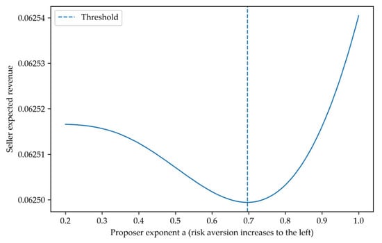
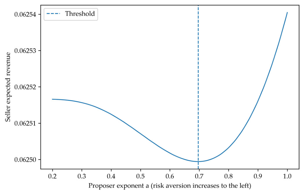
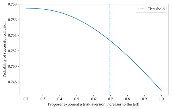
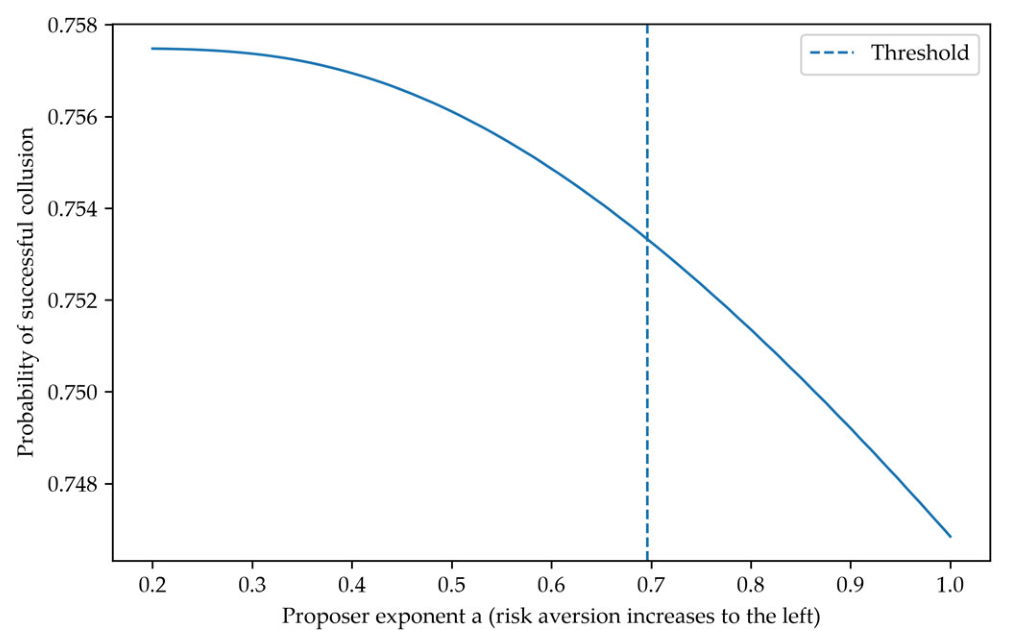
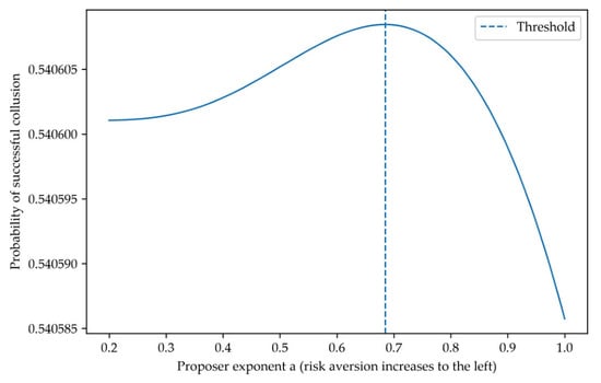
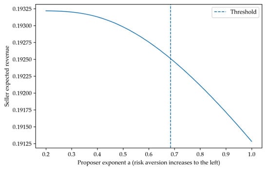
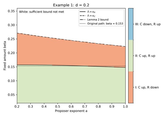
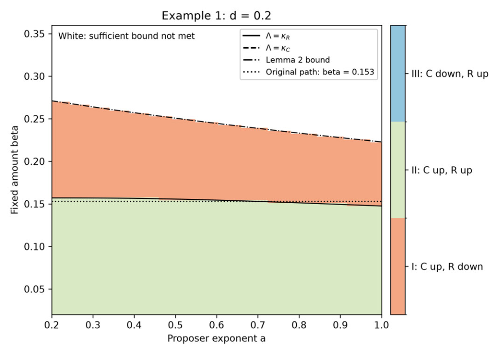
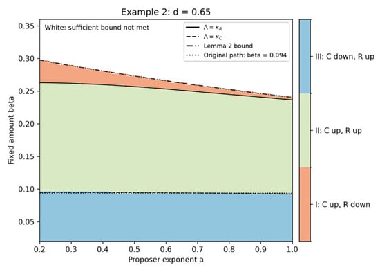
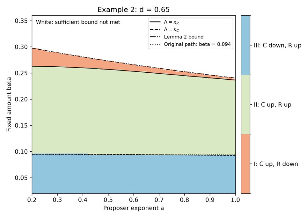
Disclaimer/Publisher’s Note: The statements, opinions and data contained in all publications are solely those of the individual author(s) and contributor(s) and not of MDPI and/or the editor(s). MDPI and/or the editor(s) disclaim responsibility for any injury to people or property resulting from any ideas, methods, instructions or products referred to in the content. |
© 2026 by the authors. Licensee MDPI, Basel, Switzerland. This article is an open access article distributed under the terms and conditions of the Creative Commons Attribution (CC BY) license.