Operator-Inequality Defects in Transform-Based Tensor Algebras: Invariance and Transform Sensitivity

Abstract

Transform-based tensor algebras induced by invertible linear transforms provide a unified framework for tensor operations and spectral analysis. This paper investigates how the choice of a unitary transform affects the quantitative tightness of classical operator inequalities. We first formulate a transform-domain transfer principle for matrix trace inequalities and examine its consequences for the Golden–Thompson, Jensen-type, Klein, and Lieb inequalities. We then study the Golden–Thompson defect through its exact slice-wise decomposition. Under bounded spectral assumptions, we establish an upper estimate in terms of squared transform-domain commutators and a matching-order lower estimate for an explicit Pauli-matrix family. We further establish qualitative transform sensitivity: explicit separation results for real orthogonal transforms, including a DFT–DCT separation at $p=4$. Finally, we investigate the non-universality of transform selection and formulate commutator-energy minimization as an operator-aware surrogate objective over the orthogonal group. The framework separates algebraic invariance from transform-dependent inequality tightness without assuming general equivalence between the defect and commutator-energy objectives.

1. Introduction

Tensor algebra based on transform-induced products has become a central tool in modern multilinear analysis [1,2]. The ${\star }_M$-product framework of Kernfeld, Kilmer, and Aeron [3] defines a tensor–tensor product for any fixed invertible transform M, and the subsequent ${\star }_M$-algebra developed by Kilmer et al. [4] provides its algebraic and spectral foundations. The operator-theoretic interpretation of third-order tensors under the t-product was developed in [5]. When M is the discrete Fourier transform, this reduces to the classical t-product of Kilmer and Martin [6]. In this study, we specialize to unitary transforms $\mathrm{\Phi }$ and study operator inequalities within this established algebra. This flexibility has led to a wide range of applications [7,8], including tensor completion, robust PCA, and signal processing, where different unitary transforms induce different notions of structure and sparsity.

A fundamental feature of these frameworks is that different choices of $\mathrm{\Phi }$ lead to algebraically isomorphic tensor algebras. Consequently, the unitary transform is often viewed as a change in basis that does not alter intrinsic properties. However, this viewpoint overlooks an important phenomenon:

(Transform-dependent noncommutativity) The choice of transform Φ defines a coordinate system in which noncommutativity is measured, and different unitary transforms reveal fundamentally different commutative structures.

This observation suggests that while algebraic properties may be invariant, quantitative behavior can depend strongly on $\mathrm{\Phi }$. The goal of this paper is to develop a systematic theory of this phenomenon in the context of classical operator inequalities.

Classical operator inequalities for matrices—including the Golden–Thompson inequality [9,10] and related Jensen-, Klein-, and Lieb-type inequalities [11]—play a foundational role in matrix analysis and operator theory. Related inequalities for t-product tensors have been studied in [12,13]. Their significance lies not only in their validity, but also in how their defect (slack) reflects noncommutativity. A natural question arises in the tensor setting: Does the choice of unitary transform Φ affect operator inequalities, or is it merely a change of basis?

At the algebraic level, the answer is straightforward: operator inequalities remain valid for all $\mathrm{\Phi }$ with exactly the same constants as in the matrix case. The algebraic structure of the ${\star }_M$ algebra is already well understood [3,4]. Our starting point is the observation that this algebraic invariance conceals a deeper phenomenon: Algebraic invariance does not imply quantitative invariance.

While operator inequalities remain valid under all unitary transforms, their defect depends explicitly on transform-domain noncommutativity. For two tensors of the same size, we write $\mathcal{A}{\oplus }_{\mathrm{\Phi }}\mathcal{B}$ for the tensor whose transform-domain lifting is the sum of the corresponding liftings:

$${\overline{\mathcal{A}{\oplus }_{\mathrm{\Phi }}\mathcal{B}}}_{\mathrm{\Phi }}={\overline{\mathcal{A}}}_{\mathrm{\Phi }}+{\overline{\mathcal{B}}}_{\mathrm{\Phi }}.$$

Since the transform is linear, this operation coincides with ordinary tensor addition. To formalize this phenomenon, we introduce the $\mathrm{\Phi }$-dependent Golden–Thompson defect

$$\begin{array}{c}\hfill {\Delta }_{\mathrm{\Phi }}(\mathcal{A},\mathcal{B}):={Tr}_{\mathrm{\Phi }}\left({\exp }_{\mathrm{\Phi }}\left(\mathcal{A}\right){\star }_{\mathrm{\Phi }}{\exp }_{\mathrm{\Phi }}\left(\mathcal{B}\right)\right)-{Tr}_{\mathrm{\Phi }}\left({\exp }_{\mathrm{\Phi }}\left(\mathcal{A}{\oplus }_{\mathrm{\Phi }}\mathcal{B}\right)\right),\end{array}$$

(1)

where $\mathcal{A},\mathcal{B}\in {\mathbb{C}}^{n\times n\times p}$ are $\mathrm{\Phi }$-Hermitian tensors whose transformed slices ${\widehat{\mathcal{A}}}_{\mathrm{\Phi }}^{\left(\omega \right)}$ and ${\widehat{\mathcal{B}}}_{\mathrm{\Phi }}^{\left(\omega \right)}$ are Hermitian for $\omega =1,\dots ,p$ (see Definition 4), ${Tr}_{\mathrm{\Phi }}(·)$ and ${\exp }_{\mathrm{\Phi }}(·)$ are the $\mathrm{\Phi }$-trace and $\mathrm{\Phi }$-exponential maps (see Definitions 2 and 3), and ${\star }_{\mathrm{\Phi }}(·,·)$ is the ${\star }_{\mathrm{\Phi }}$-product between two tensors (see Definition 1). The quantity ${\Delta }_{\mathrm{\Phi }}(\mathcal{A},\mathcal{B})$ measures the failure of exact commutativity in the transform-based tensor algebra and quantifies the deviation between multiplicative and additive spectral propagation under the $\mathrm{\Phi }$-exponential map. Under a bounded spectral-domain assumption, we show that this defect is quantitatively controlled by the aggregate transform-domain commutator energy:

$${\displaystyle \sum _{\omega =1}^p}{∥\left[{\widehat{\mathcal{A}}}_{\mathrm{\Phi }}^{\left(\omega \right)},{\widehat{\mathcal{B}}}_{\mathrm{\Phi }}^{\left(\omega \right)}\right]∥}_F^2.$$

A central consequence of this viewpoint is that no transform is universally optimal. While certain transforms, such as the discrete Fourier transform, may yield vanishing defect for specific tensor pairs, other transforms, such as the discrete cosine transform, may produce significantly smaller defects for different tensor configurations. Thus, optimal transform selection is inherently data-dependent. In this sense, the choice of $\mathrm{\Phi }$ is not merely a change of basis, but rather a choice of spectral coordinate system that determines how commutativity is evaluated in the transform domain.

The main contributions of this paper are summarized as follows:

• (Established foundation) We work within the transform-based ${\star }_M$ tensor algebra of Kernfeld–Kilmer–Aeron [3] and its ${\star }_M$-algebra formulation [4], specialized to unitary transforms $\mathrm{\Phi }$.
• (Operator-inequality transfer principle) Classical trace inequalities, including Golden–Thompson, Jensen, Klein, and Lieb, transfer to the transform-based tensor algebra with the same constants as in the matrix case.
• (Defect characterization) Under a bounded spectral-domain assumption, the Golden–Thompson defect ${\Delta }_{\mathrm{\Phi }}(\mathcal{A},\mathcal{B})$ is quantitatively controlled by the transform-domain commutator energy:

  $${\displaystyle \sum _{\omega =1}^p}{∥\left[{\widehat{\mathcal{A}}}_{\mathrm{\Phi }}^{\left(\omega \right)},{\widehat{\mathcal{B}}}_{\mathrm{\Phi }}^{\left(\omega \right)}\right]∥}_F^2.$$
• (Transform sensitivity) The Golden–Thompson defect depends nontrivially on the choice of the unitary transform $\mathrm{\Phi }$. For certain tensor pairs, choosing $\mathrm{\Phi }$ as the discrete Fourier transform (DFT) yields exact slice-wise commutativity in the transform domain, providing

  $${\Delta }_{\mathrm{DFT}}(\mathcal{A},\mathcal{B})=0.$$
  In contrast, choosing $\mathrm{\Phi }$ as the discrete cosine transform (DCT) may produce significant transform-domain noncommutativity, leading to a strictly positive defect in suitable regimes. This demonstrates that transform selection fundamentally affects the geometry of noncommutativity in the transform-based tensor algebra.
• (Non-universality and operator-aware transform selection) No unitary transform minimizes the Golden–Thompson defect for all tensor pairs. Optimal transforms are necessarily data-dependent. Transform selection can be formulated as minimizing transform-domain noncommutativity over the orthogonal group, thereby connecting the problem to approximate joint diagonalization of tensor slices.

These results establish that $\mathrm{\Phi }$ induces a nontrivial geometry of inequality tightness, governed by transform-dependent noncommutativity. To the best of our knowledge, this is the first work that separates algebraic invariance from quantitative behavior in transform-based tensor algebras.

The organization of this paper is as follows. Section 2 introduces the transform-based tensor algebra and notation. Section 3 establishes the operator-inequality transfer principle. Section 4 develops the transform-sensitive defect theory, including quantitative bounds and separation results. Section 5 investigates optimization formulations for operator-aware transform selection. Section 6 contains concluding remarks and discusses broader implications and connections to numerical linear algebra and operator theory.

2. The Transform-Based Tensor Algebra

This section recalls the transform-based tensor algebra that underlies the operator-inequality analysis in the remainder of the paper. The tensor product used here is the established ${\star }_M$-product of Kernfeld, Kilmer, and Aeron [3] and its ${\star }_M$-algebra formulation [4], specialized to unitary transforms $\mathrm{\Phi }\in {\mathbb{C}}^{p\times p}$. We denote the resulting product by ${\star }_{\mathrm{\Phi }}$ and refer to it as the ${\star }_{\mathrm{\Phi }}$-product, or simply the $\mathrm{\Phi }$-product when the transform is clear from context. We then recall the associated block-diagonal representation and the basic operations—trace, exponential, and logarithm—that will be used to state and analyze operator inequalities in later sections.

2.1. Definition of the ${\star }_{\mathrm{\Phi }}$-Product and Basic Operations

Let $\mathcal{A}\in {\mathbb{C}}^{n_1\times n_2\times p}$. For a unitary transform $\mathrm{\Phi }\in {\mathbb{C}}^{p\times p}$, define the transformed tensor ${\widehat{\mathcal{A}}}_{\mathrm{\Phi }}\in {\mathbb{C}}^{n_1\times n_2\times p}$ by applying $\mathrm{\Phi }$ to each tube (i.e., each third-mode fiber) of $\mathcal{A}$. Denote by ${\widehat{\mathcal{A}}}_{\mathrm{\Phi }}^{\left(i\right)}\in {\mathbb{C}}^{n_1\times n_2}$ the i-th frontal slice of ${\widehat{\mathcal{A}}}_{\mathrm{\Phi }}$. The associated block-diagonal matrix ${\overline{\mathcal{A}}}_{\mathrm{\Phi }}\in {\mathbb{C}}^{p{n}_1\times p{n}_2}$ is defined as

$${\overline{\mathcal{A}}}_{\mathrm{\Phi }}=blockdiag\left({\widehat{\mathcal{A}}}_{\mathrm{\Phi }}^{\left(1\right)},{\widehat{\mathcal{A}}}_{\mathrm{\Phi }}^{\left(2\right)},\dots ,{\widehat{\mathcal{A}}}_{\mathrm{\Phi }}^{\left(p\right)}\right).$$

Definition 1

(${\star }_{\mathrm{\Phi }}$-product, following [3,4]). For $\mathcal{A}\in {\mathbb{C}}^{n_1\times n_2\times p}$ and $\mathcal{B}\in {\mathbb{C}}^{n_2\times n_3\times p}$, the ${\star }_{\mathrm{\Phi }}$-product $\mathcal{C}=\mathcal{A}{\star }_{\mathrm{\Phi }}\mathcal{B}\in {\mathbb{C}}^{n_1\times n_3\times p}$ is defined by

$${\overline{\mathcal{C}}}_{\mathrm{\Phi }}={\overline{\mathcal{A}}}_{\mathrm{\Phi }}·{\overline{\mathcal{B}}}_{\mathrm{\Phi }},$$

where ${\overline{\mathcal{C}}}_{\mathrm{\Phi }}$ is the block-diagonal matrix constructed from the transformed tensor ${\widehat{\mathcal{C}}}_{\mathrm{\Phi }}$ in the same manner as above. This is the ${\star }_M$-product of [3,4] with $M=\mathrm{\Phi }$.

Remark 1.

When Φ is the discrete Fourier transform (DFT) matrix, the ${\star }_{\mathrm{\Phi }}$-product reduces to the conventional t-product of Kilmer and Martin [6]. More generally, for an invertible transform M, the construction above coincides with the transform-based tensor–tensor product of [3].

2.2. $\mathrm{\Phi }$-Trace, $\mathrm{\Phi }$-Exponential, and $\mathrm{\Phi }$-Logarithm

Definition 2

($\mathrm{\Phi }$-trace). Let $\mathcal{A}\in {\mathbb{C}}^{n\times n\times p}$. The Φ-trace of $\mathcal{A}$ is defined by

$${Tr}_{\mathrm{\Phi }}\left(\mathcal{A}\right):=Tr\left({\overline{\mathcal{A}}}_{\mathrm{\Phi }}\right),$$

where $Tr(·)$ denotes the standard matrix trace.

Definition 3

($\mathrm{\Phi }$-exponential and $\mathrm{\Phi }$-logarithm). Let $\mathcal{A}\in {\mathbb{C}}^{n\times n\times p}$ be Φ-Hermitian. The Φ-exponential and Φ-logarithm are defined via the block-diagonal lifting as

$${\exp }_{\mathrm{\Phi }}\left(\mathcal{A}\right):={\mathrm{\Phi }}^H\left[\exp \left({\overline{\mathcal{A}}}_{\mathrm{\Phi }}\right)\right],{\log }_{\mathrm{\Phi }}\left(\mathcal{A}\right):={\mathrm{\Phi }}^H\left[\log \left({\overline{\mathcal{A}}}_{\mathrm{\Phi }}\right)\right],$$

where the functions $\exp (·)$ and $\log (·)$ are applied blockwise to ${\overline{\mathcal{A}}}_{\mathrm{\Phi }}$, i.e., to each diagonal block ${\widehat{\mathcal{A}}}_{\mathrm{\Phi }}^{\left(i\right)}$.

Here, ${\mathrm{\Phi }}^H[·]$ denotes the inverse transform applied to each mode-3 fiber, i.e., the inverse of the map $\mathcal{X}\mapsto {\widehat{\mathcal{X}}}_{\mathrm{\Phi }}$. It does not denote ordinary matrix multiplication of ${\mathrm{\Phi }}^H$ with the block-diagonal matrix.

2.3. $\mathrm{\Phi }$-Hermitian Structure, Commutator, and Spectral Mapping

Definition 4

($\mathrm{\Phi }$-Hermitian). Let $\mathcal{A}\in {\mathbb{C}}^{n\times n\times p}$. We say that $\mathcal{A}$ is Φ-Hermitian if its block-diagonal lifting ${\overline{\mathcal{A}}}_{\mathrm{\Phi }}$ is Hermitian, i.e.,

$${\overline{\mathcal{A}}}_{\mathrm{\Phi }}^H={\overline{\mathcal{A}}}_{\mathrm{\Phi }}.$$

Equivalently, each transformed frontal slice ${\widehat{\mathcal{A}}}_{\mathrm{\Phi }}^{\left(i\right)}$ is Hermitian for all $i=1,\dots ,p$.

Definition 5

($\mathrm{\Phi }$-commutator). Let $\mathcal{A},\mathcal{B}$ be tensors of compatible sizes. The Φ-commutator is defined by

$${[\mathcal{A},\mathcal{B}]}_{\mathrm{\Phi }}:={\overline{\mathcal{A}}}_{\mathrm{\Phi }}{\overline{\mathcal{B}}}_{\mathrm{\Phi }}-{\overline{\mathcal{B}}}_{\mathrm{\Phi }}{\overline{\mathcal{A}}}_{\mathrm{\Phi }},$$

where the right-hand side is the ordinary matrix commutator.

Lemma 1

(Spectral mapping). Let $\mathcal{A}\in {\mathbb{C}}^{n\times n\times p}$ be Φ-Hermitian, and let f be an analytic function defined on an open set containing the spectrum of ${\overline{\mathcal{A}}}_{\mathrm{\Phi }}$. Then,

$$f_{\mathrm{\Phi }}\left(\mathcal{A}\right)={\mathrm{\Phi }}^H\left[f\left({\overline{\mathcal{A}}}_{\mathrm{\Phi }}\right)\right],$$

where $f\left({\overline{\mathcal{A}}}_{\mathrm{\Phi }}\right)$ is applied blockwise to each diagonal block. This is the standard functional calculus in the transform-domain representation of the ${\star }_M$ algebra [3,4].

Proof. 

Since $\mathcal{A}$ is $\mathrm{\Phi }$-Hermitian, the matrix ${\overline{\mathcal{A}}}_{\mathrm{\Phi }}$ is Hermitian and hence unitarily diagonalizable. Thus, there exists a unitary matrix U such that

$${\overline{\mathcal{A}}}_{\mathrm{\Phi }}=U\mathrm{\Lambda }{U}^H,$$

where $\mathrm{\Lambda }$ is diagonal containing the eigenvalues of ${\overline{\mathcal{A}}}_{\mathrm{\Phi }}$.

Using the standard functional calculus for Hermitian matrices,

$$f\left({\overline{\mathcal{A}}}_{\mathrm{\Phi }}\right)=Uf\left(\mathrm{\Lambda }\right)U^H,$$

where $f\left(\mathrm{\Lambda }\right)$ is obtained by applying f to each diagonal entry.

By definition of the $\mathrm{\Phi }$-functional calculus (cf. Section 2.2),

$$f_{\mathrm{\Phi }}\left(\mathcal{A}\right)={\mathrm{\Phi }}^H\left[f\left({\overline{\mathcal{A}}}_{\mathrm{\Phi }}\right)\right],$$

which establishes the claim.    □

Remark 2.

The Φ-Hermitian condition is essential for the spectral mapping lemma, as it guarantees that ${\overline{\mathcal{A}}}_{\mathrm{\Phi }}$ is unitarily diagonalizable with real eigenvalues. For non-Hermitian tensors, the exponential and logarithm remain well-defined via the blockwise matrix exponential and logarithm, but the spectral interpretation (e.g., eigenvalue mapping) does not hold in general.

3. An Operator-Inequality Transfer Principle

This section records a transfer principle for classical operator inequalities in the transform-based tensor algebra. The purpose of this section is two-fold. First, we recall that the standard trace inequalities—including Golden–Thompson, Jensen, Klein, and Lieb—transfer to the transform-based tensor algebra with the same constants as in the matrix case. Second, we emphasize that this transfer is a direct consequence of the established transform-domain representation of the ${\star }_M$ algebra [3,4]; it is therefore not the main contribution of this study. The main contribution, developed in Section 4, concerns the quantitative behavior of the associated defect under a change of transform.

3.1. Transfer Principle

The following transfer principle separates the algebraic validity of a matrix inequality from its quantitative behavior under a change in transform. Its purpose is to identify which conclusions follow directly from the established block-diagonal representation before examining the transform-dependent defect in Section 4.

Theorem 1

(Operator-inequality transfer principle). Let $\mathcal{I}(X_1,\dots ,X_m)$ be a trace or functional inequality that is preserved under finite direct sums of matrices. More precisely, assume that for all Hermitian matrices $X_1,\dots ,X_m$ of compatible sizes, the inequality $\mathcal{I}(X_1,\dots ,X_m)\ge 0$ holds, and that the same inequality holds for finite direct sums

$$\mathcal{I}\left({\displaystyle \underset{i=1}{\overset{p}{⨁}}}{X}_1^{\left(i\right)},\dots ,{\displaystyle \underset{i=1}{\overset{p}{⨁}}}{X}_m^{\left(i\right)}\right)\ge 0$$

whenever $\mathcal{I}(X_1^{\left(i\right)},\dots ,X_m^{\left(i\right)})\ge 0$ for each i.

Then, for every unitary transform $\mathrm{\Phi }\in {\mathbb{C}}^{p\times p}$, the corresponding inequality holds in the transform-based tensor algebra slice-wise. In particular, if ${\mathcal{A}}_1,\dots ,{\mathcal{A}}_m\in {\mathbb{C}}^{n\times n\times p}$ are Φ-Hermitian tensors, then

$${\mathcal{I}}_{\mathrm{\Phi }}({\mathcal{A}}_1,\dots ,{\mathcal{A}}_m)\ge 0,$$

where ${\mathcal{I}}_{\mathrm{\Phi }}$ denotes the Φ-lift of $\mathcal{I}$ obtained by replacing matrix operations with their Φ-counterparts.

Proof. 

Using Proposition 1, the transform-based tensor algebra is isomorphic to the block-diagonal matrix algebra

$${\mathcal{D}}_{\mathrm{\Phi }}=\left\{blockdiag(X_1,\dots ,X_p):X_i\in {\mathbb{C}}^{n\times n}\right\}.$$

Under this isomorphism, every $\mathrm{\Phi }$-Hermitian tensor $\mathcal{A}$ corresponds to a block-diagonal Hermitian matrix:

$${\overline{\mathcal{A}}}_{\mathrm{\Phi }}=blockdiag\left({\widehat{\mathcal{A}}}_{\mathrm{\Phi }}^{\left(1\right)},\dots ,{\widehat{\mathcal{A}}}_{\mathrm{\Phi }}^{\left(p\right)}\right).$$

Since the inequality $\mathcal{I}$ is preserved under finite direct sums, it holds blockwise for each slice tuple $({\widehat{\mathcal{A}}}_1^{\left(\omega \right)},\dots ,{\widehat{\mathcal{A}}}_m^{\left(\omega \right)})$, $\omega =1,\dots ,p$: applying $\mathcal{I}$ to the direct sum ${⨁}_{\omega =1}^p({\widehat{\mathcal{A}}}_1^{\left(\omega \right)},\dots ,{\widehat{\mathcal{A}}}_m^{\left(\omega \right)})$ and using the direct-sum preservation yields $\mathcal{I}\left({⨁}_{\omega }{\widehat{\mathcal{A}}}_1^{\left(\omega \right)},\dots ,{⨁}_{\omega }{\widehat{\mathcal{A}}}_m^{\left(\omega \right)}\right)\ge 0$. For trace inequalities, the trace of a block-diagonal matrix is the sum of the traces of its blocks, so this blockwise inequality is equivalent to ${\sum }_{\omega =1}^p\mathcal{I}({\widehat{\mathcal{A}}}_1^{\left(\omega \right)},\dots ,{\widehat{\mathcal{A}}}_m^{\left(\omega \right)})\ge 0$, which is exactly ${\mathcal{I}}_{\mathrm{\Phi }}({\mathcal{A}}_1,\dots ,{\mathcal{A}}_m)\ge 0$.    □

Because the block-diagonal functional calculus acts independently on each transformed slice, the matrix inequality applies to every block. For trace inequalities, the block contributions are additive. Therefore, summing the valid slice-wise inequalities establishes the tensor trace inequality:

$${\mathcal{I}}_{\mathrm{\Phi }}({\mathcal{A}}_1,\dots ,{\mathcal{A}}_m)={\displaystyle \sum _{\omega =1}^p}\mathcal{I}\left({\widehat{\mathcal{A}}}_1^{\left(\omega \right)},\dots ,{\widehat{\mathcal{A}}}_m^{\left(\omega \right)}\right)\ge 0.$$

This argument uses only the algebraic representation and the direct-sum property; it does not imply that the numerical slack of the inequality is invariant under changes of the transform.

Remark 3.

The transfer principle is a direct consequence of the standard transform-domain representation of the ${\star }_M$ algebra [3,4]. Its role here is not to establish new inequalities, but to fix the algebraic setting in which the transform-dependent defect is analyzed in Section 4.

3.2. Corollaries: Golden–Thompson, Jensen, Klein, and Lieb

We now record the four classical inequalities as corollaries of Theorem 1. Throughout, ${\oplus }_{\mathrm{\Phi }}$ denotes the $\mathrm{\Phi }$-sum, i.e.,

$${\overline{\mathcal{A}{\oplus }_{\mathrm{\Phi }}\mathcal{B}}}_{\mathrm{\Phi }}={\overline{\mathcal{A}}}_{\mathrm{\Phi }}+{\overline{\mathcal{B}}}_{\mathrm{\Phi }}.$$

Corollary 1

($\mathrm{\Phi }$-Golden–Thompson inequality). Let $\mathcal{A},\mathcal{B}\in {\mathbb{C}}^{n\times n\times p}$ be Φ-Hermitian. Then,

$${Tr}_{\mathrm{\Phi }}\left({\exp }_{\mathrm{\Phi }}\left(\mathcal{A}{\oplus }_{\mathrm{\Phi }}\mathcal{B}\right)\right)\le {Tr}_{\mathrm{\Phi }}\left({\exp }_{\mathrm{\Phi }}\left(\mathcal{A}\right){\star }_{\mathrm{\Phi }}{\exp }_{\mathrm{\Phi }}\left(\mathcal{B}\right)\right).$$

Proof. 

Apply Theorem 1 to the classical Golden–Thompson inequality,

$$Tr\left(e^{A+B}\right)\le Tr\left(e^A{e}^B\right),$$

which holds for all Hermitian matrices $A,B$ and is preserved under finite direct sums. Replacing A and B by the block-diagonal lifts ${\overline{\mathcal{A}}}_{\mathrm{\Phi }}$ and ${\overline{\mathcal{B}}}_{\mathrm{\Phi }}$ yields the claim.    □

Corollary 2

($\mathrm{\Phi }$-Jensen inequality). Let $\varphi :\mathbb{R}\to \mathbb{R}$ be a convex function with $\varphi \left(0\right)=0$. If $\mathcal{A}\in {\mathbb{C}}^{n\times n\times p}$ is Φ-Hermitian, then

$${Tr}_{\mathrm{\Phi }}\left(\varphi \left(\mathcal{A}\right)\right)\ge 0.$$

In the scalar case $n=p=1$, the inequality reduces to $\varphi \left(a\right)\ge 0$ for $a\in \mathbb{R}$, which follows from convexity and $\varphi \left(0\right)=0$. No normalization by $np$ is involved, and the previous counterexample $\varphi \left(x\right)=x$ with $\mathrm{\Phi }\mathcal{A}=-1\mathrm{\Phi }$ is excluded by the hypothesis $\varphi \left(0\right)=0$.

Proof. 

Apply Theorem 1 to the classical Jensen trace inequality $Tr\left(\varphi \right(A\left)\right)\ge 0$ for Hermitian A and convex $\varphi$ with $\varphi \left(0\right)=0$, which is preserved under finite direct sums. Replacing A by the block-diagonal lift ${\overline{\mathcal{A}}}_{\mathrm{\Phi }}$ yields $Tr\left(\varphi \left({\overline{\mathcal{A}}}_{\mathrm{\Phi }}\right)\right)\ge 0$. Since ${Tr}_{\mathrm{\Phi }}\left(\varphi \left(\mathcal{A}\right)\right)=Tr\left(\varphi \left({\overline{\mathcal{A}}}_{\mathrm{\Phi }}\right)\right)$, the claim follows.    □

Corollary 3

($\mathrm{\Phi }$-Klein inequality). Let ϕ be a convex function. If $\mathcal{A},\mathcal{B}\in {\mathbb{C}}^{n\times n\times p}$ are Φ-Hermitian, then

$${Tr}_{\mathrm{\Phi }}\left(\varphi \left(\mathcal{A}\right)-\varphi \left(\mathcal{B}\right)-(\mathcal{A}-\mathcal{B}){\varphi }^{\prime }\left(\mathcal{B}\right)\right)\ge 0.$$

Proof. 

Apply Theorem 1 to the classical Klein inequality for Hermitian matrices.    □

Corollary 4

($\mathrm{\Phi }$-Lieb concavity). The function

$$(\mathcal{A},\mathcal{B})⟼{Tr}_{\mathrm{\Phi }}\left({\exp }_{\mathrm{\Phi }}\left({\log }_{\mathrm{\Phi }}\left(\mathcal{A}\right)+{\log }_{\mathrm{\Phi }}\left(\mathcal{B}\right)\right)\right)$$

is jointly concave for $\mathcal{A}{\succ }_{\mathrm{\Phi }}0$ and $\mathcal{B}{\succ }_{\mathrm{\Phi }}0$. In the scalar case $n=p=1$, the map reduces to $(a,b)\mapsto ab$ on $a,b>0$. This map is not jointly concave in the naive sense, but the classical Lieb theorem is stated for the equivalent reformulation $(A,B)\mapsto Tr\left(A^r{B}^{1-r}\right)$ with $r\in [0,1]$, which is jointly concave; the present statement follows this standard formulation.

Proof. 

Apply Theorem 1 to Lieb’s classical joint concavity theorem for positive definite matrices, which states that $(A,B)\mapsto Tr\exp (\log A+\log B)$ is jointly concave on the cone of positive definite matrices (equivalently, $(A,B)\mapsto Tr\left(A^r{B}^{1-r}\right)$ is jointly concave for $r\in [0,1]$). Replacing $A,B$ with the block-diagonal lifts ${\overline{\mathcal{A}}}_{\mathrm{\Phi }},{\overline{\mathcal{B}}}_{\mathrm{\Phi }}$ and using ${Tr}_{\mathrm{\Phi }}(·)=Tr\left({\overline{·}}_{\mathrm{\Phi }}\right)$ yields the claim.    □

Remark 4.

Corollaries 1–4 show that the classical matrix trace inequalities transfer to transform-based tensor algebra with the same constants as in the matrix setting, independent of the choice of unitary transform Φ. This invariance follows from the transform-domain representation of the ${\star }_M$ algebra [3,4]. However, as we shall see in Section 4, the quantitative tightness of these inequalities—specifically the Golden–Thompson defect—is not invariant and depends critically on the choice of Φ.

3.3. Background: Transform-Domain Representation

For completeness, we recall the transform-domain representation that underlies Theorem 1. This representation is standard in the ${\star }_M$-algebra literature [3,4]; we state it here only to fix notation and to make the subsequent defect analysis self-contained.

Proposition 1

(Transform-domain representation, cf. [3,4]). Let

$${\mathcal{T}}_{\mathrm{\Phi }}:=\left({\mathbb{C}}^{n\times n\times p},{\star }_{\mathrm{\Phi }}\right)$$

denote the transform-based tensor algebra associated with the unitary transform Φ. Then, the mapping

$${\mathrm{\Psi }}_{\mathrm{\Phi }}:{\mathcal{T}}_{\mathrm{\Phi }}\to {\mathcal{D}}_{\mathrm{\Phi }}:=\left\{blockdiag(X_1,\dots ,X_p):X_i\in {\mathbb{C}}^{n\times n}\right\},{\mathrm{\Psi }}_{\mathrm{\Phi }}\left(\mathcal{A}\right)={\overline{\mathcal{A}}}_{\mathrm{\Phi }},$$

is an algebra isomorphism. That is,

1. 

${\mathrm{\Psi }}_{\mathrm{\Phi }}\left(\mathcal{A}{\star }_{\mathrm{\Phi }}\mathcal{B}\right)={\mathrm{\Psi }}_{\mathrm{\Phi }}\left(\mathcal{A}\right){\mathrm{\Psi }}_{\mathrm{\Phi }}\left(\mathcal{B}\right)$,

2. 

${\mathrm{\Psi }}_{\mathrm{\Phi }}$ is bijective.

Proof. 

The map ${\mathrm{\Psi }}_{\mathrm{\Phi }}$ is linear because the mode-3 transform and block-diagonal assembly are linear.

By the definition of the ${\star }_{\mathrm{\Phi }}$-product, ${\mathrm{\Psi }}_{\mathrm{\Phi }}\left(\mathcal{A}{\star }_{\mathrm{\Phi }}\mathcal{B}\right)={\mathrm{\Psi }}_{\mathrm{\Phi }}\left(\mathcal{A}\right){\mathrm{\Psi }}_{\mathrm{\Phi }}\left(\mathcal{B}\right)$, so ${\mathrm{\Psi }}_{\mathrm{\Phi }}$ preserves multiplication.

If ${\mathrm{\Psi }}_{\mathrm{\Phi }}\left(\mathcal{A}\right)=0$, every transformed frontal slice of $\mathcal{A}$ vanishes; since $\mathrm{\Phi }$ is invertible, $\mathcal{A}=0$, proving injectivity.

Conversely, for any block-diagonal matrix $X=blockdiag(X_1,\dots ,X_p)$, form a transformed tensor with frontal slices $X_1,\dots ,X_p$ and apply the inverse mode-3 transform. The resulting tensor $\mathcal{A}$ satisfies ${\mathrm{\Psi }}_{\mathrm{\Phi }}\left(\mathcal{A}\right)=X$; hence, ${\mathrm{\Psi }}_{\mathrm{\Phi }}$ is surjective.

Therefore, ${\mathrm{\Psi }}_{\mathrm{\Phi }}$ is an algebra isomorphism.    □

Remark 5

(Limits of the representation). The representation ${\mathrm{\Psi }}_{\mathrm{\Phi }}$ preserves algebraic structure and functional calculus, which explains the transfer results above. However, it does not preserve all quantitative properties of interest. In particular, the tightness of the Golden–Thompson inequality—measured by the defect ${\Delta }_{\mathrm{\Phi }}(\mathcal{A},\mathcal{B})$—depends critically on the choice of Φ. This sensitivity arises because the representation, while preserving the product, does not preserve the commutativity structure of the tensor slices in the transform domain. Different transforms Φ reveal different levels of noncommutativity, leading to transform-dependent defect magnitudes. We analyze this sensitivity in Section 4.

4. Transform-Dependent Golden–Thompson Defect

Having fixed the algebraic setting in Section 3, we now isolate the quantitative object whose transform dependence is the subject of this paper. The section proceeds in three steps: the slice-wise reduction in the defect (Lemma 2), the bounded-spectral upper and lower estimates (Theorem 2), and the qualitative separation results (Theorems 3 and 4).

4.1. Golden–Thompson Defect

The classical Golden–Thompson inequality is tight when the two matrices commute. In the transform-based tensor setting, the gap between the two sides of the inequality quantifies the effect of noncommutativity in the transform domain. This gap is the central object of our sensitivity analysis.

Definition 6

(Golden–Thompson defect). Let $\mathcal{A},\mathcal{B}\in {\mathbb{C}}^{n\times n\times p}$ be Φ-Hermitian tensors. The Golden–Thompson defect is defined by

$${\Delta }_{\mathrm{\Phi }}(\mathcal{A},\mathcal{B}):={Tr}_{\mathrm{\Phi }}\left({\exp }_{\mathrm{\Phi }}\left(\mathcal{A}\right){\star }_{\mathrm{\Phi }}{\exp }_{\mathrm{\Phi }}\left(\mathcal{B}\right)\right)-{Tr}_{\mathrm{\Phi }}\left({\exp }_{\mathrm{\Phi }}\left(\mathcal{A}{\oplus }_{\mathrm{\Phi }}\mathcal{B}\right)\right).$$

Using Corollary 1, we have

$${\Delta }_{\mathrm{\Phi }}(\mathcal{A},\mathcal{B})\ge 0.$$

Remark 6

(Role of the defect). The defect ${\Delta }_{\mathrm{\Phi }}(\mathcal{A},\mathcal{B})$ is the natural measure of inequality tightness for three reasons:

1. 

It vanishes exactly when $\mathcal{A}$ and $\mathcal{B}$ commute in the transform domain, i.e., $[{\overline{\mathcal{A}}}_{\mathrm{\Phi }},{\overline{\mathcal{B}}}_{\mathrm{\Phi }}]=0$.

2. 

It is quantitatively controlled by the transform-domain commutator.

3. 

It is sensitive to the choice of Φ, making it the right objective for operator-aware transform selection.

4.2. Main Theorem: Transform-Sensitive Defect

We now formalize the central phenomenon of this work: while operator inequalities in the transform-based tensor algebra transfer with the same constants as in the matrix case, their defect exhibits quantitative dependence on transform-domain noncommutativity.

Lemma 2

(Slice-wise reduction of the defect). Let $\mathcal{A},\mathcal{B}\in {\mathbb{C}}^{n\times n\times p}$ be Φ-Hermitian tensors. Under the transform-domain representation ${\mathrm{\Psi }}_{\mathrm{\Phi }}\left(\mathcal{A}\right)={\overline{\mathcal{A}}}_{\mathrm{\Phi }}$ of Proposition 1, the Golden–Thompson defect decomposes as a sum of slice-wise classical defects:

$${\Delta }_{\mathrm{\Phi }}(\mathcal{A},\mathcal{B})={\displaystyle \sum _{\omega =1}^p}\left(Tr\left(e^{A_{\omega }}{e}^{B_{\omega }}\right)-Tr\left(e^{A_{\omega }+B_{\omega }}\right)\right),$$

where $A_{\omega }:={\widehat{\mathcal{A}}}_{\mathrm{\Phi }}^{\left(\omega \right)}$ and $B_{\omega }:={\widehat{\mathcal{B}}}_{\mathrm{\Phi }}^{\left(\omega \right)}$ are Hermitian matrices.

Proof. 

Using the definitions of ${Tr}_{\mathrm{\Phi }}$, ${\exp }_{\mathrm{\Phi }}$, ${\star }_{\mathrm{\Phi }}$, and ${\oplus }_{\mathrm{\Phi }}$, and the representation ${\mathrm{\Psi }}_{\mathrm{\Phi }}$ from Proposition 1,

$${\Delta }_{\mathrm{\Phi }}(\mathcal{A},\mathcal{B})=Tr\left(e^{{\overline{\mathcal{A}}}_{\mathrm{\Phi }}}{e}^{{\overline{\mathcal{B}}}_{\mathrm{\Phi }}}\right)-Tr\left(e^{{\overline{\mathcal{A}}}_{\mathrm{\Phi }}+{\overline{\mathcal{B}}}_{\mathrm{\Phi }}}\right).$$

Since ${\overline{\mathcal{A}}}_{\mathrm{\Phi }}$ and ${\overline{\mathcal{B}}}_{\mathrm{\Phi }}$ are block-diagonal with diagonal blocks $A_{\omega }$ and $B_{\omega }$, the trace decomposes as a sum over blocks. The exponential of a block-diagonal matrix is block-diagonal with exponentials of each block. Hence,

$${\Delta }_{\mathrm{\Phi }}(\mathcal{A},\mathcal{B})={\displaystyle \sum _{\omega =1}^p}\left(Tr\left(e^{A_{\omega }}{e}^{B_{\omega }}\right)-Tr\left(e^{A_{\omega }+B_{\omega }}\right)\right).$$

The Hermiticity of $A_{\omega }$ and $B_{\omega }$ follows from the $\mathrm{\Phi }$-Hermitian assumption. This completes the proof.    □

Theorem 2

(Transform-sensitive defect under bounded spectral domain). Let $\mathcal{A},\mathcal{B}\in {\mathbb{C}}^{n\times n\times p}$ be Φ-Hermitian tensors, and assume that there exists $R>0$, such that

$$\parallel {\widehat{\mathcal{A}}}_{\mathrm{\Phi }}^{\left(\omega \right)}{\parallel }_2\le R,{\parallel {\widehat{\mathcal{B}}}_{\mathrm{\Phi }}^{\left(\omega \right)}\parallel }_2\le R\forall \omega =1,\dots ,p.$$

Then, the following statements hold.

(i) 

(Upper bound) There exists a constant $C_R>0$, depending only on R, such that

$${\Delta }_{\mathrm{\Phi }}(\mathcal{A},\mathcal{B})\le C_R{\displaystyle \sum _{\omega =1}^p}{∥[{\widehat{\mathcal{A}}}_{\mathrm{\Phi }}^{\left(\omega \right)},{\widehat{\mathcal{B}}}_{\mathrm{\Phi }}^{\left(\omega \right)}]∥}_F^2.$$

(ii) 

(Matching-order lower bound on an explicit family) For every $R>0$ there exist ${\epsilon }_0\left(R\right)>0$ and a one-parameter family ${({\mathcal{A}}_{\epsilon },{\mathcal{B}}_{\epsilon })}_{0<\epsilon <{\epsilon }_0\left(R\right)}$ in the bounded spectral class, such that

$${\Delta }_{\mathrm{\Phi }}({\mathcal{A}}_{\epsilon },{\mathcal{B}}_{\epsilon })\ge c_R{\displaystyle \sum _{\omega =1}^p}{\parallel [{\widehat{\mathcal{A}}}_{\mathrm{\Phi },\epsilon }^{\left(\omega \right)},{\widehat{\mathcal{B}}}_{\mathrm{\Phi },\epsilon }^{\left(\omega \right)}]\parallel }_F^2$$

for some $c_R>0$. This lower estimate is asserted only for the constructed family.

(iii) 

(Transform sensitivity) There exist tensors $\mathcal{A},\mathcal{B}$ and unitary transforms ${\mathrm{\Phi }}_1,{\mathrm{\Phi }}_2\in {\mathbb{C}}^{p\times p}$, such that

$${\Delta }_{{\mathrm{\Phi }}_1}(\mathcal{A},\mathcal{B})=0,{\Delta }_{{\mathrm{\Phi }}_2}(\mathcal{A},\mathcal{B})>0.$$

(iv) 

(Vanishing condition) If

$$[{\widehat{\mathcal{A}}}_{\mathrm{\Phi }}^{\left(\omega \right)},{\widehat{\mathcal{B}}}_{\mathrm{\Phi }}^{\left(\omega \right)}]=0,\forall \omega =1,\dots ,p,$$

then

$${\Delta }_{\mathrm{\Phi }}(\mathcal{A},\mathcal{B})=0.$$

Consequently, on the bounded spectral class $\parallel {\widehat{\mathcal{A}}}_{\mathrm{\Phi }}^{\left(\omega \right)}{\parallel }_2,{\parallel {\widehat{\mathcal{B}}}_{\mathrm{\Phi }}^{\left(\omega \right)}\parallel }_2\le R$, the defect satisfies the upper bound in (i) for all admissible tensors, and the lower bound in (ii) on the one-parameter family ${({\mathcal{A}}_{\epsilon },{\mathcal{B}}_{\epsilon })}_{0<\epsilon <{\epsilon }_0\left(R\right)}$ constructed in the proof of (ii). For this family, the two-sided estimate

$$c_R{\displaystyle \sum _{\omega =1}^p}{∥[{\widehat{\mathcal{A}}}_{\mathrm{\Phi }}^{\left(\omega \right)},{\widehat{\mathcal{B}}}_{\mathrm{\Phi }}^{\left(\omega \right)}]∥}_F^2\le {\Delta }_{\mathrm{\Phi }}(\mathcal{A},\mathcal{B})\le C_R{\displaystyle \sum _{\omega =1}^p}{∥[{\widehat{\mathcal{A}}}_{\mathrm{\Phi }}^{\left(\omega \right)},{\widehat{\mathcal{B}}}_{\mathrm{\Phi }}^{\left(\omega \right)}]∥}_F^2$$

holds on the explicit family of part (ii). A general lower bound valid for all tensors in the bounded spectral class is not claimed; see Remark 7.

Proof. 

Using Lemma 2, we obtain the slice-wise decomposition

$${\Delta }_{\mathrm{\Phi }}(\mathcal{A},\mathcal{B})={\displaystyle \sum _{\omega =1}^p}\delta (A_{\omega },B_{\omega }),$$

where

$$\delta (A,B):=Tr\left(e^A{e}^B\right)-Tr\left(e^{A+B}\right)\ge 0$$

is the classical Golden–Thompson defect for Hermitian matrices, and $A_{\omega }={\widehat{\mathcal{A}}}_{\mathrm{\Phi }}^{\left(\omega \right)}$, $B_{\omega }={\widehat{\mathcal{B}}}_{\mathrm{\Phi }}^{\left(\omega \right)}$.

Part (i): Upper bound. For Hermitian matrices $A,B$ with ${\parallel A\parallel }_2,{\parallel B\parallel }_2\le R$, classical quantitative versions of the Golden–Thompson inequality (see, e.g., [14]) provide a constant of $C_R>0$, depending only on R, such that

$$\delta (A,B)\le C_R{\parallel [A,B]\parallel }_F^2.$$

Applying this to each slice pair $(A_{\omega },B_{\omega })$ and summing over $\omega =1,\dots ,p$ yields

$${\Delta }_{\mathrm{\Phi }}(\mathcal{A},\mathcal{B})\le C_R{\displaystyle \sum _{\omega =1}^p}{\parallel [A_{\omega },B_{\omega }]\parallel }_F^2,$$

which establishes part (i).

Part (ii): Lower bound. For every transformed slice, choose $A_{\omega }=\epsilon {\sigma }_x$, $B_{\omega }=\epsilon {\sigma }_z$, where

$${\sigma }_x=\left(\begin{array}{cc}0& 1\\ 1& 0\end{array}\right),{\sigma }_z=\left(\begin{array}{cc}1& 0\\ 0& -1\end{array}\right).$$

Since ${\sigma }_x^2={\sigma }_z^2=I$ and ${\sigma }_x{\sigma }_z+{\sigma }_z{\sigma }_x=0$,

$$e^{A_{\omega }}=\cosh \epsilon I+\sinh \epsilon {\sigma }_x,e^{B_{\omega }}=\cosh \epsilon I+\sinh \epsilon {\sigma }_z,$$

so

$$e^{A_{\omega }}{e}^{B_{\omega }}={\cosh }^2\epsilon I+\cosh \epsilon \sinh \epsilon {\sigma }_x+\cosh \epsilon \sinh \epsilon {\sigma }_z+{\sinh }^2\epsilon {\sigma }_x{\sigma }_z.$$

Taking traces and using $TrI=2$, $Tr{\sigma }_x=Tr{\sigma }_z=0$, $Tr\left({\sigma }_x{\sigma }_z\right)=0$,

$$Tr\left(e^{A_{\omega }}{e}^{B_{\omega }}\right)=2{\cosh }^2\epsilon .$$

Since ${\sigma }_x+{\sigma }_z$ is Hermitian with eigenvalues $\pm \sqrt{2}$,

$$Tr\left(e^{A_{\omega }+B_{\omega }}\right)=2\cosh \left(\sqrt{2}\epsilon \right).$$

Hence,

$$\delta (A_{\omega },B_{\omega })=2{\cosh }^2\epsilon -2\cosh \left(\sqrt{2}\epsilon \right)={\displaystyle \frac{{\epsilon }^4}{3}}+{\displaystyle \frac{{\epsilon }^6}{15}}+O\left({\epsilon }^8\right).$$

Moreover, $[A_{\omega },B_{\omega }]=2i{\epsilon }^2{\sigma }_y$ and $\parallel {\sigma }_y{\parallel }_F^2=2$, so $\parallel [A_{\omega },B_{\omega }]{\parallel }_F^2=8{\epsilon }^4$. Therefore,

$$\delta (A_{\omega },B_{\omega })={\displaystyle \frac{1}{24}}{\parallel [A_{\omega },B_{\omega }]\parallel }_F^2+O\left({\epsilon }^6\right).$$

For sufficiently small positive $\epsilon$, there exists $c_R>0$, such that $\delta (A_{\omega },B_{\omega })\ge c_R{\parallel [A_{\omega },B_{\omega }]\parallel }_F^2$. Summing over $\omega$ yields the lower bound for the constructed family.

Part (iii): Transform sensitivity. Let ${\mathrm{\Phi }}_1={\mathrm{\Phi }}_{\mathrm{DFT}}$ and ${\mathrm{\Phi }}_2={\mathrm{\Phi }}_{\mathrm{DCT}}$. The qualitative separation is established in Theorems 3 and 4 below. In particular, Theorem 4 constructs tensors $\mathcal{A},\mathcal{B}$, such that all slices commute in the DFT domain and hence ${\Delta }_{{\mathrm{\Phi }}_1}(\mathcal{A},\mathcal{B})=0$, while the DCT domain produces a strictly positive defect, i.e., ${\Delta }_{{\mathrm{\Phi }}_2}(\mathcal{A},\mathcal{B})>0$. The continuity of $\mathrm{\Phi }\mapsto {\Delta }_{\mathrm{\Phi }}(\mathcal{A},\mathcal{B})$ follows from the facts:

• ${\widehat{\mathcal{A}}}_{\mathrm{\Phi }}^{\left(\omega \right)}$ and ${\widehat{\mathcal{B}}}_{\mathrm{\Phi }}^{\left(\omega \right)}$ depend linearly on $\mathrm{\Phi }$;
• the matrix exponential and trace are continuous;
• the unitary group $\mathcal{U}\left(p\right)$ is compact.

Thus, the mapping is continuous and therefore locally Lipschitz on compact subsets of $\mathcal{U}\left(p\right)$.

Part (iv): Vanishing condition. If $[A_{\omega },B_{\omega }]=0$ for all $\omega$, then each pair $(A_{\omega },B_{\omega })$ consists of commuting Hermitian matrices. Commuting Hermitian matrices are simultaneously diagonalizable, which implies

$$e^{A_{\omega }}{e}^{B_{\omega }}=e^{A_{\omega }+B_{\omega }}.$$

Hence, $\delta (A_{\omega },B_{\omega })=0$ for each $\omega$. Summing over $\omega$ and applying Lemma 2 yields ${\Delta }_{\mathrm{\Phi }}(\mathcal{A},\mathcal{B})=0$.

This completes the proof of Theorem 2.    □

Remark 7

(Scope of the lower bound). Part (ii) establishes the lower bound only on the explicitly constructed one-parameter family. All subsequent statements that invoke a two-sided estimate are to be read as restricted to this family, or are reformulated as surrogate statements in Section 5.

Remark 8.

The constants $C_R$ and $c_R$ in Theorem 2 depend only on the spectral bound R, not on the tensor dimensions n and p or on the specific choice of Φ. This bounded spectral-domain formulation avoids the use of a universal constant, which would be inconsistent with the exponential scaling of the Golden–Thompson defect under rescaling $A\mapsto tA$, $B\mapsto tB$.

Remark 9.

On the bounded spectral class of Theorem 2, ${\Delta }_{\mathrm{\Phi }}$ defines a non-negative, transform-dependent functional on the admissible transform space, whose magnitude is bounded above by the squared commutator energy under the bounded spectral assumption of Theorem 2(i). This endows the unitary group $\mathcal{U}\left(p\right)$ with a noncommutativity geometry; ${\Delta }_{\mathrm{\Phi }}$ is not asserted to be a quadratic functional of Φ.

4.3. Qualitative Transform Separation: DFT vs. DCT

We now construct an explicit example showing that the Golden–Thompson defect can differ dramatically between two standard transforms. This example demonstrates that algebraic invariance does not imply quantitative invariance.

Theorem 3

(Explicit separation for real orthogonal transforms). Let $p\ge 2$ and let ${\mathrm{\Phi }}_1,{\mathrm{\Phi }}_2\in O\left(p\right)$ be real orthogonal transforms, such that

$$U:={\mathrm{\Phi }}_2{\mathrm{\Phi }}_1^{\top }$$

is not a signed permutation matrix. Then, there exist tensors $\mathcal{A},\mathcal{B}\in {\mathbb{R}}^{n\times n\times p}$ (with $n\ge 2$) that are both ${\mathrm{\Phi }}_1$-Hermitian and ${\mathrm{\Phi }}_2$-Hermitian and satisfy

$${\Delta }_{{\mathrm{\Phi }}_1}(\mathcal{A},\mathcal{B})=0,{\Delta }_{{\mathrm{\Phi }}_2}(\mathcal{A},\mathcal{B})>0.$$

Proof. 

Step 1: A row of U with two nonzero entries. Since $U\in O\left(p\right)$ and U is not a signed permutation matrix, U has a row containing at least two nonzero entries. Indeed, if every row of U had exactly one nonzero entry, then, since each row of an orthogonal matrix has unit Euclidean norm, that entry would have modulus 1; the rows would then be distinct standard basis vectors, so U would be a signed permutation matrix, contradicting the hypothesis. Hence, there exist a row index r and distinct column indices $j\ne k$, such that $U_{rj}\ne 0$ and $U_{rk}\ne 0$.

Step 2: Choice of noncommuting Hermitian matrices. Let

$$H_1=\left(\begin{array}{cc}0& 1\\ 1& 0\end{array}\right),H_2=\left(\begin{array}{cc}1& 0\\ 0& -1\end{array}\right),$$

embedded in the upper-left $2\times 2$ block of an $n\times n$ matrix and zero-padded elsewhere. Then, $H_1,H_2$ are real symmetric and

$$[H_1,H_2]=2i{\sigma }_y\ne 0,{\sigma }_y=\left(\begin{array}{cc}0& -i\\ i& 0\end{array}\right),$$

so $[H_1,H_2]\ne 0$.

Step 3: Construction of the ${\mathrm{\Phi }}_1$-domain slices. Choose $\lambda \in \mathbb{R}\setminus \left\{1\right\}$ (e.g., $\lambda =2$). Define frontal slices ${\widehat{\mathcal{A}}}_{{\mathrm{\Phi }}_1}^{\left(\omega \right)}$ and ${\widehat{\mathcal{B}}}_{{\mathrm{\Phi }}_1}^{\left(\omega \right)}$ for $\omega =1,\dots ,p$ by

$${\widehat{\mathcal{A}}}_{{\mathrm{\Phi }}_1}^{\left(j\right)}=H_1,{\widehat{\mathcal{B}}}_{{\mathrm{\Phi }}_1}^{\left(j\right)}=H_1,$$

$${\widehat{\mathcal{A}}}_{{\mathrm{\Phi }}_1}^{\left(k\right)}=H_2,{\widehat{\mathcal{B}}}_{{\mathrm{\Phi }}_1}^{\left(k\right)}=\lambda H_2,$$

and ${\widehat{\mathcal{A}}}_{{\mathrm{\Phi }}_1}^{\left(\omega \right)}={\widehat{\mathcal{B}}}_{{\mathrm{\Phi }}_1}^{\left(\omega \right)}=0$ for all other $\omega$.

Define the physical tensors by the inverse mode-3 transform:

$$\mathcal{A}:={\mathrm{\Phi }}_1^H\left[{\widehat{\mathcal{A}}}_{{\mathrm{\Phi }}_1}\right],\mathcal{B}:={\mathrm{\Phi }}_1^H\left[{\widehat{\mathcal{B}}}_{{\mathrm{\Phi }}_1}\right].$$

Because ${\mathrm{\Phi }}_1$ is real orthogonal, ${\mathrm{\Phi }}_1^H={\mathrm{\Phi }}_1^{\top }$ is real, so $\mathcal{A},\mathcal{B}$ are real tensors.

Step 4: ${\mathrm{\Phi }}_1$-Hermiticity and ${\mathrm{\Phi }}_2$-Hermiticity. Every slice ${\widehat{\mathcal{A}}}_{{\mathrm{\Phi }}_1}^{\left(\omega \right)}$ and ${\widehat{\mathcal{B}}}_{{\mathrm{\Phi }}_1}^{\left(\omega \right)}$ is either 0, $H_1$, $H_2$, or $\lambda H_2$, and hence, real symmetric. Therefore, ${\overline{\mathcal{A}}}_{{\mathrm{\Phi }}_1}$ and ${\overline{\mathcal{B}}}_{{\mathrm{\Phi }}_1}$ are block-diagonal with real symmetric blocks, and hence, Hermitian; this is exactly ${\mathrm{\Phi }}_1$-Hermiticity.

For ${\mathrm{\Phi }}_2$-Hermiticity, we use the slice-wise mixing formula. For every $\omega$,

$${\widehat{\mathcal{A}}}_{{\mathrm{\Phi }}_2}^{\left(\omega \right)}={\displaystyle \sum _{\mathsf{\ell }=1}^p}{U}_{\omega \mathsf{\ell }}{\widehat{\mathcal{A}}}_{{\mathrm{\Phi }}_1}^{\left(\mathsf{\ell }\right)},{\widehat{\mathcal{B}}}_{{\mathrm{\Phi }}_2}^{\left(\omega \right)}={\displaystyle \sum _{\mathsf{\ell }=1}^p}{U}_{\omega \mathsf{\ell }}{\widehat{\mathcal{B}}}_{{\mathrm{\Phi }}_1}^{\left(\mathsf{\ell }\right)}.$$

Since U is real and every ${\widehat{\mathcal{A}}}_{{\mathrm{\Phi }}_1}^{\left(\mathsf{\ell }\right)}$ and ${\widehat{\mathcal{B}}}_{{\mathrm{\Phi }}_1}^{\left(\mathsf{\ell }\right)}$ is real symmetric, each transformed slice ${\widehat{\mathcal{A}}}_{{\mathrm{\Phi }}_2}^{\left(\omega \right)}$ and ${\widehat{\mathcal{B}}}_{{\mathrm{\Phi }}_2}^{\left(\omega \right)}$ is a real linear combination of real symmetric matrices, hence real symmetric. Therefore, $\mathcal{A},\mathcal{B}$ are ${\mathrm{\Phi }}_2$-Hermitian.

Step 5: ${\Delta }_{{\mathrm{\Phi }}_1}(\mathcal{A},\mathcal{B})=0$. For every $\omega$, the pair $({\widehat{\mathcal{A}}}_{{\mathrm{\Phi }}_1}^{\left(\omega \right)},{\widehat{\mathcal{B}}}_{{\mathrm{\Phi }}_1}^{\left(\omega \right)})$ is one of

$$(0,0),(H_1,H_1),(H_2,\lambda H_2),$$

so the two matrices are scalar multiples of a common matrix (or both zero) and, therefore, commute the following: $[{\widehat{\mathcal{A}}}_{{\mathrm{\Phi }}_1}^{\left(\omega \right)},{\widehat{\mathcal{B}}}_{{\mathrm{\Phi }}_1}^{\left(\omega \right)}]=0$ for all $\omega$. Using Theorem 2(iv), ${\Delta }_{{\mathrm{\Phi }}_1}(\mathcal{A},\mathcal{B})=0$.

Step 6: A nonzero commutator in the ${\mathrm{\Phi }}_2$ domain. Set $a:=U_{rj}$ and $b:=U_{rk}$. For the distinguished row r, only $\mathsf{\ell }=j$ and $\mathsf{\ell }=k$ contribute:

$${\widehat{\mathcal{A}}}_{{\mathrm{\Phi }}_2}^{\left(r\right)}=a{H}_1+b{H}_2,{\widehat{\mathcal{B}}}_{{\mathrm{\Phi }}_2}^{\left(r\right)}=a{H}_1+\lambda b{H}_2.$$

Their commutator is

$$\begin{array}{cc}\hfill [{\widehat{\mathcal{A}}}_{{\mathrm{\Phi }}_2}^{\left(r\right)},{\widehat{\mathcal{B}}}_{{\mathrm{\Phi }}_2}^{\left(r\right)}]& =[a{H}_1+b{H}_2,a{H}_1+\lambda b{H}_2]\hfill \\ & =a\lambda b[H_1,H_2]+ab[H_2,H_1]\hfill \\ & =ab(\lambda -1)[H_1,H_2].\hfill \end{array}$$

Since $a\ne 0$, $b\ne 0$, $\lambda \ne 1$, and $[H_1,H_2]\ne 0$, we obtain $[{\widehat{\mathcal{A}}}_{{\mathrm{\Phi }}_2}^{\left(r\right)},{\widehat{\mathcal{B}}}_{{\mathrm{\Phi }}_2}^{\left(r\right)}]\ne 0$.

Step 7: Strict positivity of ${\Delta }_{{\mathrm{\Phi }}_2}$. Using Lemma 2,

$${\Delta }_{{\mathrm{\Phi }}_2}(\mathcal{A},\mathcal{B})={\displaystyle \sum _{\omega =1}^p}\delta \left({\widehat{\mathcal{A}}}_{{\mathrm{\Phi }}_2}^{\left(\omega \right)},{\widehat{\mathcal{B}}}_{{\mathrm{\Phi }}_2}^{\left(\omega \right)}\right),$$

where $\delta (A,B)=Tr\left(e^A{e}^B\right)-Tr\left(e^{A+B}\right)$ is the classical Golden–Thompson defect for Hermitian matrices. Each summand is non-negative using the Golden–Thompson inequality. At $\omega =r$, the pair is Hermitian (by Step 4) and noncommuting (by Step 6); for Hermitian matrices, equality in the Golden–Thompson inequality holds if and only if the matrices commute; hence, $\delta ({\widehat{\mathcal{A}}}_{{\mathrm{\Phi }}_2}^{\left(r\right)},{\widehat{\mathcal{B}}}_{{\mathrm{\Phi }}_2}^{\left(r\right)})>0$. Therefore,

$${\Delta }_{{\mathrm{\Phi }}_2}(\mathcal{A},\mathcal{B})\ge \delta \left({\widehat{\mathcal{A}}}_{{\mathrm{\Phi }}_2}^{\left(r\right)},{\widehat{\mathcal{B}}}_{{\mathrm{\Phi }}_2}^{\left(r\right)}\right)>0.$$

This completes the proof.    □

Theorem 4

(Explicit DFT–DCT separation). For $p=4$, there exist real tensors $\mathcal{A},\mathcal{B}\in {\mathbb{R}}^{2\times 2\times 4}$ whose physical frontal slices are symmetric, such that

$${\Delta }_{\mathrm{DFT}}(\mathcal{A},\mathcal{B})=0,{\Delta }_{\mathrm{DCT}}(\mathcal{A},\mathcal{B})>0.$$

Proof. 

Let $H_1={\sigma }_x$ and $H_2={\sigma }_z$, i.e.,

$$H_1=\left(\begin{array}{cc}0& 1\\ 1& 0\end{array}\right),H_2=\left(\begin{array}{cc}1& 0\\ 0& -1\end{array}\right).$$

Using zero-based frequency indices, prescribe the DFT-domain slices by

$$A_0=H_2,B_0=2H_2,A_1=A_3=B_1=B_3=H_1,A_2=B_2=0.$$

These arrays satisfy the conjugate-symmetry conditions $A_{\omega }=\overline{A_{4-\omega }}$ and $B_{\omega }=\overline{B_{4-\omega }}$ (for $\omega =0,1,2,3$), so their inverse DFT yields real symmetric physical frontal slices.

A direct computation, recorded in Appendix A, shows that the second DCT-domain slice pair is

$$A_1^{\prime }=c{H}_1+s{H}_2,B_1^{\prime }=c{H}_1+2s{H}_2,$$

where

$$c=\cos (\pi /8),s=\sin (\pi /8).$$

Consequently,

$$[A_1^{\prime },B_1^{\prime }]=cs[H_1,H_2]\ne 0.$$

All DCT-domain slices are real symmetric because they are real linear combinations of the real symmetric physical frontal slices. The strict equality condition in the Golden–Thompson inequality therefore yields

$$\delta (A_1^{\prime },B_1^{\prime })>0.$$

All remaining slice defects are non-negative. Using Lemma 2,

$${\Delta }_{\mathrm{DCT}}(\mathcal{A},\mathcal{B})\ge \delta (A_1^{\prime },B_1^{\prime })>0.$$

This completes the proof.    □

Remark 10

(Scope of the DFT–DCT construction). Theorem 4 presents an explicit analytical witness for $p=4$ under the orthonormal DFT and DCT-II conventions. It shows that the specific real-symmetric Pauli construction of Theorem 3 is not the only admissible route: using conjugate-paired DFT-domain slices allows the complex mixing coefficients to combine into real symmetric DCT-domain slices while preserving noncommutativity. Whether the construction extends to all p, or to other transform pairs, remains open. In particular, for general p the DCT-domain slices are obtained from the DFT-domain slices via the mixing matrix $U={\mathrm{\Phi }}_{\mathrm{DCT}}{\mathrm{\Phi }}_{\mathrm{DFT}}^H$, and the individual terms $U_{\omega k}{U}_{\omega \mathsf{\ell }}[{\widehat{\mathcal{A}}}_{\mathrm{DFT}}^{\left(k\right)},{\widehat{\mathcal{B}}}_{\mathrm{DFT}}^{\left(\mathsf{\ell }\right)}]$ in the resulting commutator can in principle cancel; the explicit computation in Appendix A rules out such cancellation only for $p=4$. The general-orthogonal construction of Theorem 3 avoids this issue by using a single row of U with exactly two nonzero entries, but it does not specialize to the DFT–DCT pair. A general-p DFT–DCT qualitative separation, or a general non-cancellation theorem for $U={\mathrm{\Phi }}_{\mathrm{DCT}}{\mathrm{\Phi }}_{\mathrm{DFT}}^H$, is left open; the conditional quantitative statement in Theorem 5 makes the required non-cancellation property an explicit hypothesis.

For the construction of Theorem 4, the DCT-domain slice pair $(A_1^{\prime },B_1^{\prime })$ satisfies $\parallel [A_1^{\prime },B_1^{\prime }]{\parallel }_F=cs{\parallel [H_1,H_2]\parallel }_F>0$ and $\parallel A_1^{\prime }{\parallel }_2,{\parallel B_1^{\prime }\parallel }_2\le R$ for a suitable R, so the non-degeneracy hypothesis of Theorem 5 is satisfied with $n=2$ and $p=4$.

Remark 11

(On quantitative separation). A stronger quantitative separation of the form ${\Delta }_{\mathrm{DCT}}(\mathcal{A},\mathcal{B})\ge cp$ requires additional structural assumptions on the mixing matrix $U={\mathrm{\Phi }}_{\mathrm{DCT}}{\mathrm{\Phi }}_{\mathrm{DFT}}^H$, such as a non-cancellation property of its entries across opposite-parity indices. We state such a quantitative result conditionally in Theorem 5 below; verifying the required non-cancellation property for specific transform pairs is left as a separate question.

Theorem 5

(Conditional quantitative separation). Consider a sequence of tensor pairs $({\mathcal{A}}_p,{\mathcal{B}}_p)$ with transformed slices of fixed matrix dimension n, and two unitary transforms ${\mathrm{\Phi }}_{1,p},{\mathrm{\Phi }}_{2,p}\in {\mathbb{C}}^{p\times p}$, such that ${\mathcal{A}}_p,{\mathcal{B}}_p$ are both ${\mathrm{\Phi }}_{1,p}$-Hermitian and ${\mathrm{\Phi }}_{2,p}$-Hermitian. Suppose that

$${\Delta }_{{\mathrm{\Phi }}_{1,p}}({\mathcal{A}}_p,{\mathcal{B}}_p)=0.$$

Assume that there exist constants $\eta >0$, $R>0$, and $\alpha >0$, all independent of p, and a subset $S_p\subseteq \{1,\dots ,p\}$ with $|S_p|\ge \alpha p$ such that for every $\omega \in S_p$,

$${∥[{\widehat{\mathcal{A}}}_{{\mathrm{\Phi }}_{2,p}}^{\left(\omega \right)},{\widehat{\mathcal{B}}}_{{\mathrm{\Phi }}_{2,p}}^{\left(\omega \right)}]∥}_F\ge \eta ,\parallel {\widehat{\mathcal{A}}}_{{\mathrm{\Phi }}_{2,p}}^{\left(\omega \right)}{\parallel }_2\le R,{\parallel {\widehat{\mathcal{B}}}_{{\mathrm{\Phi }}_{2,p}}^{\left(\omega \right)}\parallel }_2\le R.$$

Then, there exist constants $d_0=d_0(n,R,\eta )>0$ and $c>0$, independent of p, such that

$$\delta \left({\widehat{\mathcal{A}}}_{{\mathrm{\Phi }}_{2,p}}^{\left(\omega \right)},{\widehat{\mathcal{B}}}_{{\mathrm{\Phi }}_{2,p}}^{\left(\omega \right)}\right)\ge d_0\forall \omega \in S_p,$$

and hence, ${\Delta }_{{\mathrm{\Phi }}_{2,p}}({\mathcal{A}}_p,{\mathcal{B}}_p)\ge cp$.

Proof. 

Step 1: Uniform positivity on the compact set. Let

$$\mathcal{K}:=\left\{(A,B)\in {\mathbb{H}}_n\times {\mathbb{H}}_n{:\parallel A\parallel }_2\le {R,\parallel B\parallel }_2\le R,{\parallel [A,B]\parallel }_F\ge \eta \right\},$$

where ${\mathbb{H}}_n$ is the space of $n\times n$ Hermitian matrices. The set $\mathcal{K}$ is closed and bounded, and hence compact. The map

$$(A,B)\mapsto \delta (A,B)=Tr\left(e^A{e}^B\right)-Tr\left(e^{A+B}\right)$$

is continuous on $\mathcal{K}$. For Hermitian matrices, the Golden–Thompson defect $\delta (A,B)$ is non-negative, and it vanishes if and only if $[A,B]=0$. Since ${\parallel [A,B]\parallel }_F\ge \eta >0$ on $\mathcal{K}$, we have $\delta (A,B)>0$ for every $(A,B)\in \mathcal{K}$. By compactness,

$$d_0:=d_0(n,R,\eta ):=\underset{(A,B)\in \mathcal{K}}{\min }\delta (A,B)>0.$$

Step 2: Linear lower bound. Since ${\mathcal{A}}_p,{\mathcal{B}}_p$ are ${\mathrm{\Phi }}_{2,p}$-Hermitian, Lemma 2 yields

$${\Delta }_{{\mathrm{\Phi }}_{2,p}}({\mathcal{A}}_p,{\mathcal{B}}_p)={\displaystyle \sum _{\omega =1}^p}\delta \left({\widehat{\mathcal{A}}}_{{\mathrm{\Phi }}_{2,p}}^{\left(\omega \right)},{\widehat{\mathcal{B}}}_{{\mathrm{\Phi }}_{2,p}}^{\left(\omega \right)}\right).$$

Each summand is non-negative. For $\omega \in S_p$, the corresponding slice pair belongs to $\mathcal{K}$, so $\delta ({\widehat{\mathcal{A}}}_{{\mathrm{\Phi }}_{2,p}}^{\left(\omega \right)},{\widehat{\mathcal{B}}}_{{\mathrm{\Phi }}_{2,p}}^{\left(\omega \right)})\ge d_0$. Hence,

$${\Delta }_{{\mathrm{\Phi }}_{2,p}}({\mathcal{A}}_p,{\mathcal{B}}_p)\ge \sum _{\omega \in S_p}{d}_0=\left|S_p\right|d_0\ge \alpha d_{0}p.$$

Setting $c:=\alpha d_0>0$ completes the proof.

Remark on the role of the hypothesis ${\Delta }_{{\mathrm{\Phi }}_{1,p}}=0$. This hypothesis is used only to ensure that the separation is nontrivial, i.e., that ${\mathrm{\Phi }}_{1,p}$ achieves zero defect while ${\mathrm{\Phi }}_{2,p}$ is strictly suboptimal. The linear lower bound itself depends only on the ${\mathrm{\Phi }}_{2,p}$-domain non-degeneracy and on the ${\mathrm{\Phi }}_{2,p}$-Hermiticity of ${\mathcal{A}}_p,{\mathcal{B}}_p$.    □

Remark 12

(Failure of the hypotheses of Theorems 5 and 6). The hypothesis $\parallel [{\widehat{\mathcal{A}}}_{{\mathrm{\Phi }}_{2,p}}^{\left(\omega \right)},$${\widehat{\mathcal{B}}}_{{\mathrm{\Phi }}_{2,p}}^{\left(\omega \right)}{]\parallel }_F\ge \eta$ with $\eta >0$ independent of p is essential and can fail. For instance, take ${\widehat{\mathcal{A}}}_{{\mathrm{\Phi }}_{2,p}}^{\left(\omega \right)}={\epsilon }_p{H}_1$ and ${\widehat{\mathcal{B}}}_{{\mathrm{\Phi }}_{2,p}}^{\left(\omega \right)}={\epsilon }_p{H}_2$ with ${\epsilon }_p\to 0$ as $p\to \infty$. Then, the commutator norm equals ${\epsilon }_p^2{\parallel [H_1,H_2]\parallel }_F\to 0$, so no uniform $\eta >0$ exists, and the compactness argument of Theorem 5 cannot be applied. In this regime, one can only conclude ${\Delta }_{{\mathrm{\Phi }}_{2,p}}({\mathcal{A}}_p,{\mathcal{B}}_p)\to 0$, not a linear-in-p lower bound.

The same construction illustrates the failure of the hypothesis of Theorem 6 (dimension-preserving embedding). That theorem requires a pair $({\mathcal{A}}^{\left(2\right)},{\mathcal{B}}^{\left(2\right)})$ that is ${\mathrm{\Phi }}_1$-Hermitian and ${\mathrm{\Phi }}_2$-Hermitian and satisfies ${\Delta }_{{\mathrm{\Phi }}_1}=0$, ${\Delta }_{{\mathrm{\Phi }}_2}>0$. If the relative transform $U={\mathrm{\Phi }}_2{\mathrm{\Phi }}_1^{\top }$ is a signed permutation matrix, then the ${\mathrm{\Phi }}_2$-domain slices are obtained from the ${\mathrm{\Phi }}_1$-domain slices by a signed permutation, so commutativity in one domain is equivalent to commutativity in the other; consequently, no such pair exists, and the embedding theorem cannot be applied. This is precisely the signed-permutation exception that appears in the hypotheses of Theorems 3 and 7.

Theorem 6

(Dimension-preserving embedding). Let ${\mathrm{\Phi }}_1,{\mathrm{\Phi }}_2\in {\mathbb{C}}^{p\times p}$ be unitary transforms. Suppose a pair ${\mathcal{A}}^{\left(2\right)},{\mathcal{B}}^{\left(2\right)}\in {\mathbb{C}}^{2\times 2\times p}$ is both ${\mathrm{\Phi }}_1$-Hermitian and ${\mathrm{\Phi }}_2$-Hermitian and satisfies

$${\Delta }_{{\mathrm{\Phi }}_1}({\mathcal{A}}^{\left(2\right)},{\mathcal{B}}^{\left(2\right)})=0,{\Delta }_{{\mathrm{\Phi }}_2}({\mathcal{A}}^{\left(2\right)},{\mathcal{B}}^{\left(2\right)})>0.$$

Then, for every $n\ge 2$, there exist tensors $\mathcal{A},\mathcal{B}\in {\mathbb{C}}^{n\times n\times p}$ with the same two defect values.

Proof. 

Embed each physical frontal slice into the upper-left $2\times 2$ block:

$${\mathcal{A}}^{\left(k\right)}=\left(\begin{array}{cc}{\mathcal{A}}^{\left(2\right),\left(k\right)}& 0\\ 0& 0_{n-2}\end{array}\right),{\mathcal{B}}^{\left(k\right)}=\left(\begin{array}{cc}{\mathcal{B}}^{\left(2\right),\left(k\right)}& 0\\ 0& 0_{n-2}\end{array}\right).$$

Because the transforms act only along the third mode, this direct-sum structure is preserved in each transform domain. For every transformed slice,

$$e^{A_{\omega }}=\left(\begin{array}{cc}{e}^{A_{\omega }^{\left(2\right)}}& 0\\ 0& I_{n-2}\end{array}\right),e^{B_{\omega }}=\left(\begin{array}{cc}{e}^{B_{\omega }^{\left(2\right)}}& 0\\ 0& I_{n-2}\end{array}\right),$$

and similarly for $e^{A_{\omega }+B_{\omega }}$. Hence,

$$Tr\left(e^{A_{\omega }}{e}^{B_{\omega }}\right)=Tr\left(e^{A_{\omega }^{\left(2\right)}}{e}^{B_{\omega }^{\left(2\right)}}\right)+(n-2),$$

$$Tr{e}^{A_{\omega }+B_{\omega }}=Tr{e}^{A_{\omega }^{\left(2\right)}+B_{\omega }^{\left(2\right)}}+(n-2).$$

The additional terms cancel in the defect, so ${\Delta }_{{\mathrm{\Phi }}_i}(\mathcal{A},\mathcal{B})={\Delta }_{{\mathrm{\Phi }}_i}({\mathcal{A}}^{\left(2\right)},{\mathcal{B}}^{\left(2\right)})$ for $i=1,2$.    □

Remark 13.

Combining Theorem 4 with Theorem 6 yields an explicit DFT–DCT separation in any matrix dimension $n\ge 2$.

4.4. Numerical Illustration

We provide a numerical illustration of the transform sensitivity predicted by the theory. Two distinct objects are involved, and we keep them separate throughout:

(i)

the explicit $p=4$ analytical witness of Theorem 4, which establishes the existence of a strict separation between DFT and DCT;

(ii)

a family of commuting DFT-domain slices parametrized by the tensor depth p, used only to visualize the empirical trend of the DCT defect as p grows.

The numerical experiment in (ii) is not the $p=4$ witness of Theorem 4; it is a separate construction whose purpose is to illustrate the qualitative phenomenon, not to verify the non-degeneracy hypothesis of Theorem 5 for all p.

The analytical $p=4$ witness. For the construction of Theorem 4, the DFT-domain slices are

$$A_0=H_2,B_0=2H_2,A_1=A_3=B_1=B_3=H_1,A_2=B_2=0,$$

with $H_1={\sigma }_x$ and $H_2={\sigma }_z$. The DCT-domain slice pair at $\omega =1$ is

$$A_1^{\prime }=c{H}_1+s{H}_2,B_1^{\prime }=c{H}_1+2s{H}_2,c=\cos (\pi /8),s=\sin (\pi /8),$$

so $[A_1^{\prime },B_1^{\prime }]=cs[H_1,H_2]\ne 0$, and hence, ${\Delta }_{\mathrm{DCT}}(\mathcal{A},\mathcal{B})>0$, while ${\Delta }_{\mathrm{DFT}}(\mathcal{A},\mathcal{B})=0$. This is a single, analytically verified data point at $p=4$; it is not a curve in p.

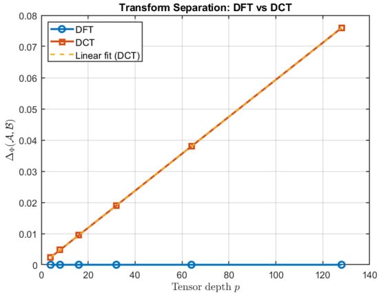
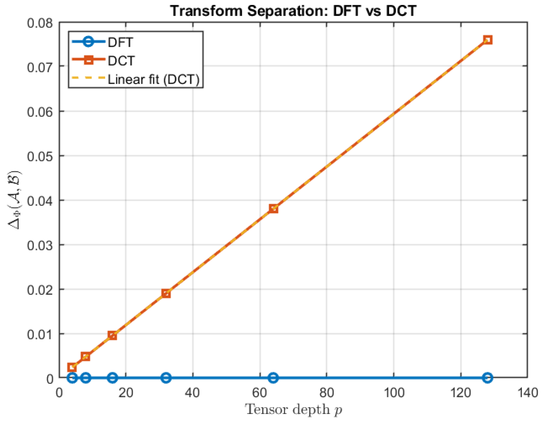
The numerical family used in Figure 1. To visualize the dependence of the defect on the tensor depth, we use a separate family of commuting DFT-domain slices, parametrized by $p\in \{4,8,16,32,64,128\}$, in which each slice pair consists of scalar multiples of a single Pauli matrix (alternating between $H_1$ and $H_2$ across the frequency index). Using Theorem 2(iv), this construction yields ${\Delta }_{\mathrm{DFT}}(\mathcal{A},\mathcal{B})\approx 0$ up to numerical precision. Evaluating the same tensors under the DCT transform produces a strictly positive defect, consistent with the qualitative separation underlying Theorem 4.

Figure 1. Transform separation under different spectral bases. The Golden–Thompson defect ${\Delta }_{\mathrm{\Phi }}(\mathcal{A},\mathcal{B})$ is plotted as a function of the tensor depth p for the DFT and DCT transforms. The DFT construction yields defects at the level of numerical precision, while the DCT transform produces a strictly positive defect that grows approximately linearly with p. The dashed line is the linear fit ${\Delta }_{\mathrm{DCT}}\approx 5.93\times {10}^{-4}p$ discussed in the text; it is almost indistinguishable from, and essentially overlaps with, the DCT defect curve over the displayed range of p, confirming that the empirical growth is approximately linear. This figure is a numerical illustration of the qualitative separation underlying Theorem 4; it is not the explicit $p=4$ witness of that theorem, and the fitted line is empirical and does not by itself establish a quantitative lower bound.

Figure 1 plots ${\Delta }_{\mathrm{\Phi }}(\mathcal{A},\mathcal{B})$ as a function of the tensor depth p for the DFT and DCT transforms. The DFT construction yields defects at the level of numerical precision, reflecting exact slice-wise commutativity in the Fourier domain. In contrast, the DCT transform produces a strictly positive defect that grows approximately linearly with p. A linear fit yields

$${\Delta }_{\mathrm{DCT}}(\mathcal{A},\mathcal{B})\approx 5.93\times {10}^{-4}p.$$

This empirical trend is consistent with the qualitative separation underlying Theorem 4; it does not verify the non-degeneracy hypothesis of Theorem 5 for all p, nor does it assert a dimension-independent quantitative lower bound. It confirms only that the inequality itself transfers to the tensor setting (Corollary 1), while its quantitative tightness depends strongly on the choice of transform.

5. Operator-Aware Transform Selection

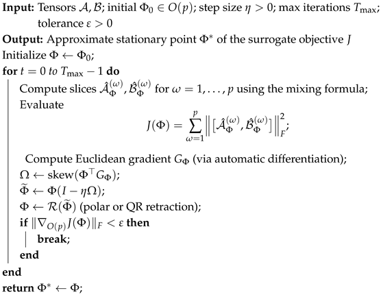
The separation results above show that a transform (e.g., DFT) can outperform another (e.g., DCT) for specific tensor pairs. This raises a fundamental question: can one identify a transform that minimizes the defect uniformly over all tensor pairs? As we show below, the answer is negative (Theorem 7), and this motivates the operator-aware formulation over $O\left(p\right)$ (Definition 7 and Corollary 5), together with the Riemannian gradient scheme (Algorithm 1).

Algorithm 1: Riemannian gradient scheme for operator-aware transform selection

The answer is negative. Transform optimality is not globally ordered: different transforms can be optimal for different data. In other words, the choice of $\mathrm{\Phi }$ is inherently data-dependent rather than universally optimal. The following theorem formalizes this non-universality.

Theorem 7

(Transform non-universality). Let ${\mathrm{\Phi }}_1,{\mathrm{\Phi }}_2\in {\mathbb{R}}^{p\times p}$ be two distinct orthogonal transforms, such that $U:={\mathrm{\Phi }}_2{\mathrm{\Phi }}_1^{\top }$ is not a signed permutation matrix. Then, the following statements hold:

1. 

There exist tensors $\mathcal{A},\mathcal{B}\in {\mathbb{C}}^{n\times n\times p}$ that are both ${\mathrm{\Phi }}_1$-Hermitian and ${\mathrm{\Phi }}_2$-Hermitian, such that

$${\Delta }_{{\mathrm{\Phi }}_1}(\mathcal{A},\mathcal{B})=0,{\Delta }_{{\mathrm{\Phi }}_2}(\mathcal{A},\mathcal{B})>0.$$

2. 

There exist tensors ${\mathcal{A}}^{\prime },{\mathcal{B}}^{\prime }\in {\mathbb{C}}^{n\times n\times p}$ that are both ${\mathrm{\Phi }}_1$-Hermitian and ${\mathrm{\Phi }}_2$-Hermitian, such that

$${\Delta }_{{\mathrm{\Phi }}_1}({\mathcal{A}}^{\prime },{\mathcal{B}}^{\prime })>0,{\Delta }_{{\mathrm{\Phi }}_2}({\mathcal{A}}^{\prime },{\mathcal{B}}^{\prime })=0.$$

In particular, no single orthogonal transform is universally optimal; the optimal transform depends on the joint structure of the tensor pair.

Proof. 

We prove the two statements separately.

Part 1: ${\mathrm{\Phi }}_1$ optimal, ${\mathrm{\Phi }}_2$ suboptimal. Let $U={\mathrm{\Phi }}_2{\mathrm{\Phi }}_1^{\top }$. Since U is not a signed permutation matrix, there exists at least one row of U containing two nonzero entries. Fix such a row index r, and choose two column indices $j\ne k$ with $U_{rj}\ne 0$ and $U_{rk}\ne 0$.

Let $H_1,H_2\in {\mathbb{C}}^{n\times n}$ be two Hermitian matrices that do not commute, i.e., $[H_1,H_2]\ne 0$. A concrete choice is the Pauli matrices ${\sigma }_x$ and ${\sigma }_z$ embedded in the upper-left $2\times 2$ block, with zeros elsewhere. This ensures that the tensors are $\mathrm{\Phi }$-Hermitian for any real orthogonal $\mathrm{\Phi }$, because the zero padding preserves Hermiticity under real linear combinations.

Construct tensors $\mathcal{A},\mathcal{B}$ by specifying their ${\mathrm{\Phi }}_1$-domain frontal slices as follows. Set all slices to zero except:

$${\widehat{\mathcal{A}}}_{{\mathrm{\Phi }}_1}^{\left(j\right)}=H_1,{\widehat{\mathcal{B}}}_{{\mathrm{\Phi }}_1}^{\left(j\right)}=H_1,$$

$${\widehat{\mathcal{A}}}_{{\mathrm{\Phi }}_1}^{\left(k\right)}=H_2,{\widehat{\mathcal{B}}}_{{\mathrm{\Phi }}_1}^{\left(k\right)}=\lambda H_2,$$

where $\lambda \in \mathbb{R}$ is a scalar with $\lambda \ne 1$ (e.g., $\lambda =2$). All other slices are set to the zero matrix.

Since ${\mathrm{\Phi }}_1$ and ${\mathrm{\Phi }}_2$ are real orthogonal, and the constructed ${\mathrm{\Phi }}_1$-domain slices are Hermitian (they are either $H_1$, $\lambda H_2$, or zero), the resulting physical tensors are both ${\mathrm{\Phi }}_1$-Hermitian and ${\mathrm{\Phi }}_2$-Hermitian. This follows because the inverse transforms ${\mathrm{\Phi }}_1^{\top }$ and ${\mathrm{\Phi }}_2^{\top }$ are also real, so Hermiticity is preserved under real linear combinations.

Now, we study the defect under ${\mathrm{\Phi }}_1$. For every slice index $\omega$, the pair $({\widehat{\mathcal{A}}}_{{\mathrm{\Phi }}_1}^{\left(\omega \right)},{\widehat{\mathcal{B}}}_{{\mathrm{\Phi }}_1}^{\left(\omega \right)})$ consists of scalar multiples of the same Hermitian matrix (or both are zero). Hence they commute:

$$[{\widehat{\mathcal{A}}}_{{\mathrm{\Phi }}_1}^{\left(\omega \right)},{\widehat{\mathcal{B}}}_{{\mathrm{\Phi }}_1}^{\left(\omega \right)}]=0\forall \omega .$$

Using Theorem 2(iv), commuting slices imply vanishing defect:

$${\Delta }_{{\mathrm{\Phi }}_1}(\mathcal{A},\mathcal{B})=0.$$

For the defect under ${\mathrm{\Phi }}_2$, the ${\mathrm{\Phi }}_2$-domain slices are obtained by mixing the ${\mathrm{\Phi }}_1$-domain slices via the matrix $U={\mathrm{\Phi }}_2{\mathrm{\Phi }}_1^{\top }$:

$${\widehat{\mathcal{A}}}_{{\mathrm{\Phi }}_2}^{\left(\omega \right)}={\displaystyle \sum _{\mathsf{\ell }=1}^p}{U}_{\omega \mathsf{\ell }}{\widehat{\mathcal{A}}}_{{\mathrm{\Phi }}_1}^{\left(\mathsf{\ell }\right)},{\widehat{\mathcal{B}}}_{{\mathrm{\Phi }}_2}^{\left(\omega \right)}={\displaystyle \sum _{\mathsf{\ell }=1}^p}{U}_{\omega \mathsf{\ell }}{\widehat{\mathcal{B}}}_{{\mathrm{\Phi }}_1}^{\left(\mathsf{\ell }\right)}.$$

For the distinguished row index r, only columns j and k contribute nonzero terms (all other slices are zero). Therefore,

$${\widehat{\mathcal{A}}}_{{\mathrm{\Phi }}_2}^{\left(r\right)}=U_{rj}{H}_1+U_{rk}{H}_2,{\widehat{\mathcal{B}}}_{{\mathrm{\Phi }}_2}^{\left(r\right)}=U_{rj}{H}_1+\lambda U_{rk}{H}_2.$$

Their commutator is

$$[{\widehat{\mathcal{A}}}_{{\mathrm{\Phi }}_2}^{\left(r\right)},{\widehat{\mathcal{B}}}_{{\mathrm{\Phi }}_2}^{\left(r\right)}]=U_{rj}{U}_{rk}(1-\lambda )[H_1,H_2]\ne 0,$$

since $U_{rj},U_{rk}\ne 0$, $\lambda \ne 1$, and $[H_1,H_2]\ne 0$.

Because this slice has a nonzero commutator, the classical Golden–Thompson defect for this slice pair is strictly positive. Using the slice-wise decomposition (Lemma 2) and the fact that the defect sums over slices with non-negative contributions, we obtain

$${\Delta }_{{\mathrm{\Phi }}_2}(\mathcal{A},\mathcal{B})>0.$$

Part 2: ${\mathrm{\Phi }}_2$ optimal, ${\mathrm{\Phi }}_1$ suboptimal. The second statement follows by symmetry. Consider the matrix $U^{\prime }={\mathrm{\Phi }}_1{\mathrm{\Phi }}_2^{\top }=U^{\top }$. Since U is not a signed permutation matrix, $U^{\top }$ is also not a signed permutation matrix. Hence, the same construction applied with the roles of ${\mathrm{\Phi }}_1$ and ${\mathrm{\Phi }}_2$ exchanged yields tensors ${\mathcal{A}}^{\prime },{\mathcal{B}}^{\prime }$, such that

$${\Delta }_{{\mathrm{\Phi }}_2}({\mathcal{A}}^{\prime },{\mathcal{B}}^{\prime })=0,{\Delta }_{{\mathrm{\Phi }}_1}({\mathcal{A}}^{\prime },{\mathcal{B}}^{\prime })>0.$$

This completes the proof. □

Remark 14

(Data-dependent optimality). Theorem 7 establishes that no fixed transform is universally optimal; the optimal ${\mathrm{\Phi }}^{*}$ depends on the joint commutativity structure of $(\mathcal{A},\mathcal{B})$. This justifies the adaptive optimization framework in Section 5, where the transform is selected from data rather than prescribed a priori.

Remark 15

(Relation to representation-oriented transform learning). The transform-selection problem considered here differs from representation-oriented transform learning, such as the matrix-mimetic algebra optimization of Newman and Keegan [15]. In [15], the transform is chosen to optimize representation, compression, or approximation properties of the algebra. In contrast, our objective is operator-aware: we select Φ to minimize transform-domain noncommutativity,

$${\displaystyle \sum _{\omega =1}^p}{∥\left[{\widehat{\mathcal{A}}}_{\mathrm{\Phi }}^{\left(\omega \right)},{\widehat{\mathcal{B}}}_{\mathrm{\Phi }}^{\left(\omega \right)}\right]∥}_F^2.$$

Hence, this improves the tightness of operator inequalities for a given tensor pair $(\mathcal{A},\mathcal{B})$.

5.1. Operator-Aware Transform Selection

Theorem 2 shows that, under a bounded spectral-domain assumption, the defect ${\Delta }_{\mathrm{\Phi }}$ is quantitatively controlled by transform-domain noncommutativity. This naturally leads to an optimization problem over the orthogonal group, where the goal is to select a transform that minimizes the defect and hence reduces noncommutativity in the transformed domain. This reveals that transform selection is equivalent to searching for a coordinate system that minimizes noncommutative interaction.

We restrict to real orthogonal transforms $\mathrm{\Phi }\in O\left(p\right)$ for two reasons. First, for real tensors whose frontal slices are symmetric, and for real orthogonal transforms, the transformed slices remain symmetric. This ensures that the optimization domain is well-defined and that $\mathrm{\Phi }$-Hermiticity is preserved along the optimization path. Second, the orthogonal group $O\left(p\right)$ is compact and admits standard Riemannian optimization techniques. The complex unitary case is discussed in Section 6.

Definition 7

(Admissible transform selection). Let $\mathcal{A},\mathcal{B}\in {\mathbb{R}}^{n\times n\times p}$ have symmetric frontal slices. Define the defect objective $D\left(\mathrm{\Phi }\right)={\Delta }_{\mathrm{\Phi }}(\mathcal{A},\mathcal{B})$ and the commutator-energy surrogate $J\left(\mathrm{\Phi }\right)={\sum }_{\omega =1}^p{\parallel [{\widehat{\mathcal{A}}}_{\mathrm{\Phi }}^{\left(\omega \right)},{\widehat{\mathcal{B}}}_{\mathrm{\Phi }}^{\left(\omega \right)}]\parallel }_F^2$ on $O\left(p\right)$. The optimal defect problem is ${\min }_{\mathrm{\Phi }\in O\left(p\right)}D\left(\mathrm{\Phi }\right)$; the surrogate problem is ${\min }_{\mathrm{\Phi }\in O\left(p\right)}J\left(\mathrm{\Phi }\right)$. These are distinct unless an additional theorem relates their minimizers.

Example 1

(Hermiticity is automatic in the real symmetric setting). If $\mathcal{A},\mathcal{B}\in {\mathbb{R}}^{n\times n\times p}$ have symmetric frontal slices and $\mathrm{\Phi }\in O\left(p\right)$ is real orthogonal, then each transformed slice is a real linear combination of symmetric matrices, and hence real symmetric. Thus, $\mathcal{A},\mathcal{B}$ are Φ-Hermitian for every $\mathrm{\Phi }\in O\left(p\right)$.

Theorem 8

(Existence and zero-defect optimality). Let $\mathcal{A},\mathcal{B}$ satisfy the assumptions of Definition 7. Then,

(i) 

Both D and J attain global minima on $O\left(p\right)$.

(ii) 

If $J\left({\mathrm{\Phi }}_0\right)=0$ for some ${\mathrm{\Phi }}_0\in O\left(p\right)$, then $D\left({\mathrm{\Phi }}_0\right)=0$, and ${\mathrm{\Phi }}_0$ is a global minimizer of both objectives.

(iii) 

If $D\left({\mathrm{\Phi }}_0\right)=0$ and equality in the Golden–Thompson inequality is characterized by commutativity for every transformed slice, then $J\left({\mathrm{\Phi }}_0\right)=0$.

(iv) 

No equality of the complete minimizer sets is claimed when their minimum values are strictly positive.

Proof. 

(i) Existence. The transformed slices depend continuously on $\mathrm{\Phi }$, and matrix exponentiation, trace, and commutator operations are continuous. Consequently, D and J are continuous on the compact group $O\left(p\right)$, and both attain their minima.

(ii) Zero-defect optimality. If $J\left({\mathrm{\Phi }}_0\right)=0$, every transformed slice pair commutes. The Golden–Thompson defect vanishes slice-wise, so $D\left({\mathrm{\Phi }}_0\right)=0$. Non-negativity of both objectives establishes global optimality.

(iii) Converse under equality characterization. If $D\left({\mathrm{\Phi }}_0\right)=0$, all non-negative slice-wise defects vanish. Under the Golden–Thompson equality characterization, each transformed slice pair commutes; hence, $J\left({\mathrm{\Phi }}_0\right)=0$.

(iv) This is a statement of scope and requires no proof. □

Corollary 5

(Commutator energy as a surrogate objective). Let $\mathcal{A},\mathcal{B}$ satisfy the bounded spectral assumption of Theorem 2, and define

$$D\left(\mathrm{\Phi }\right):={\Delta }_{\mathrm{\Phi }}(\mathcal{A},\mathcal{B}),J\left(\mathrm{\Phi }\right):=\mathcal{C}\left(\mathrm{\Phi }\right):={\displaystyle \sum _{\omega =1}^p}{∥[{\widehat{\mathcal{A}}}_{\mathrm{\Phi }}^{\left(\omega \right)},{\widehat{\mathcal{B}}}_{\mathrm{\Phi }}^{\left(\omega \right)}]∥}_F^2,\mathrm{\Phi }\in O\left(p\right).$$

Then, the following statements hold:

(i) 

(Existence) Both D and J attain global minima on $O\left(p\right)$; see Theorem 8(i).

(ii) 

(Upper surrogate bound) There exists $C_R>0$, depending only on the spectral bound R, such that

$$D\left(\mathrm{\Phi }\right)\le C_{R}J\left(\mathrm{\Phi }\right)\mathit{for}\mathit{all}\mathit{admissible}\mathrm{\Phi }\in O\left(p\right)$$

on the bounded spectral class. Consequently, for every ${\mathrm{\Phi }}_J\in {arg\; min}_{\mathrm{\Phi }\in O\left(p\right)}J\left(\mathrm{\Phi }\right)$,

$$\underset{\mathrm{\Phi }\in O\left(p\right)}{\min }D\left(\mathrm{\Phi }\right)\le D\left({\mathrm{\Phi }}_J\right)\le C_{R}J\left({\mathrm{\Phi }}_J\right)=C_R\underset{\mathrm{\Phi }\in O\left(p\right)}{\min }J\left(\mathrm{\Phi }\right).$$

Thus, J is an upper surrogate for D on this class, and minimizing J controls D up to the constant $C_R$.

(iii) 

(Matching lower bound on the explicit family at the fixed transform of Theorem 2(ii)) Let ${({\mathcal{A}}_{\epsilon },{\mathcal{B}}_{\epsilon })}_{0<\epsilon <{\epsilon }_0\left(R\right)}$ be the one-parameter Pauli family constructed in the proof of Theorem 2(ii), and let ${\mathrm{\Phi }}_0$ denote the transform with respect to which this family is constructed. By Theorem 2(ii) and Remark 7, there exists $c_R>0$, depending only on R, such that

$$D_{\epsilon }\left({\mathrm{\Phi }}_0\right)\ge c_R{J}_{\epsilon }\left({\mathrm{\Phi }}_0\right).$$

No lower bound of the form $D_{\epsilon }\left(\mathrm{\Phi }\right)\ge c_R{J}_{\epsilon }\left(\mathrm{\Phi }\right)$ is asserted for all $\mathrm{\Phi }\in O\left(p\right)$; establishing such a uniform-in-transform lower bound would require proving ${\inf }_{\mathrm{\Phi }\in O\left(p\right),J_{\epsilon }\left(\mathrm{\Phi }\right)>0}{D}_{\epsilon }\left(\mathrm{\Phi }\right)/J_{\epsilon }\left(\mathrm{\Phi }\right)>0$, which is not attempted here. No comparable lower bound is asserted for general tensors in the bounded spectral class; see Remark 7.

(iv) 

(Zero-defect case) If ${\min }_{\mathrm{\Phi }\in O\left(p\right)}J\left(\mathrm{\Phi }\right)=0$, then using Theorem 8(ii), every minimizer ${\mathrm{\Phi }}_0$ of J satisfies $D\left({\mathrm{\Phi }}_0\right)=0$, so ${\mathrm{\Phi }}_0$ is also a global minimizer of D, and the minimizer sets coincide at the zero level. This is the only regime in which an exact (not merely constant-factor) identification of minimizers is asserted.

(v) 

(Scope and interpretation) When ${\min }_{\mathrm{\Phi }\in O\left(p\right)}J\left(\mathrm{\Phi }\right)>0$, statement (ii) provides an upper surrogate bound on the bounded spectral class, and statement (iii) provides a two-sided constant-factor comparison only at the fixed transform ${\mathrm{\Phi }}_0$ of Theorem 2(ii) and on the explicit Pauli family constructed there. No equality of the full minimizer sets ${arg\; min}_{\mathrm{\Phi }\in O\left(p\right)}D\left(\mathrm{\Phi }\right)$ and ${arg\; min}_{\mathrm{\Phi }\in O\left(p\right)}J\left(\mathrm{\Phi }\right)$ is claimed in this regime; cf. Theorem 8(iv). Accordingly, minimizing ${\Delta }_{\mathrm{\Phi }}$ is analogous to finding an orthogonal transform that makes the transformed slices as commuting as possible, and J is to be regarded as a surrogate for D rather than as an equivalent objective. A precise equivalence with a standard approximate joint diagonalization criterion would require an additional theorem; we therefore present this connection as motivation rather than as an identity.

Proof. 

(i) This is Theorem 8(i); it is restated here only to fix notation for subsequent items.

(ii) Using Theorem 2(i), on the bounded spectral class there exists $C_R>0$, depending only on R, such that $D\left(\mathrm{\Phi }\right)\le C_{R}J\left(\mathrm{\Phi }\right)$ for all admissible $\mathrm{\Phi }\in O\left(p\right)$. Let ${\mathrm{\Phi }}_J\in {arg\; min}_{\mathrm{\Phi }\in O\left(p\right)}J\left(\mathrm{\Phi }\right)$, which exists by (i). Then,

$$\underset{\mathrm{\Phi }\in O\left(p\right)}{\min }D\left(\mathrm{\Phi }\right)\le D\left({\mathrm{\Phi }}_J\right)\le C_{R}J\left({\mathrm{\Phi }}_J\right)=C_R\underset{\mathrm{\Phi }\in O\left(p\right)}{\min }J\left(\mathrm{\Phi }\right).$$

This is the asserted upper surrogate bound.

(iii) Using Theorem 2(ii) and Remark 7, on the one-parameter Pauli family $({\mathcal{A}}_{\epsilon },{\mathcal{B}}_{\epsilon })$, at the fixed transform ${\mathrm{\Phi }}_0$ of Theorem 2(ii), there exists $C_R>0$, depending only on R, such that $D_{\epsilon }\left({\mathrm{\Phi }}_0\right)\ge c_R{J}_{\epsilon }\left({\mathrm{\Phi }}_0\right)$. At this fixed ${\mathrm{\Phi }}_0$, the upper bound of (ii) also holds, so

$$c_R{J}_{\epsilon }\left({\mathrm{\Phi }}_0\right)\le D_{\epsilon }\left({\mathrm{\Phi }}_0\right)\le C_R{J}_{\epsilon }\left({\mathrm{\Phi }}_0\right).$$

No statement is made about ${\min }_{\mathrm{\Phi }\in O\left(p\right)}{D}_{\epsilon }\left(\mathrm{\Phi }\right)$ or ${\min }_{\mathrm{\Phi }\in O\left(p\right)}{J}_{\epsilon }\left(\mathrm{\Phi }\right)$.

(iv) If ${\min }_{\mathrm{\Phi }}J\left(\mathrm{\Phi }\right)=0$, then any minimizer ${\mathrm{\Phi }}_0$ of J satisfies $J\left({\mathrm{\Phi }}_0\right)=0$, so every transformed slice pair commutes. By Theorem 2(iv), $D\left({\mathrm{\Phi }}_0\right)=0$; since $D\ge 0$ by Corollary 1, ${\mathrm{\Phi }}_0$ is a global minimizer of D. Conversely, if $D\left({\mathrm{\Phi }}_0\right)=0$ and the Golden–Thompson equality characterization applies slice-wise, then $J\left({\mathrm{\Phi }}_0\right)=0$ by Theorem 8(iii), so ${\mathrm{\Phi }}_0$ is a global minimizer of J. Hence the two minimizer sets agree at the zero level.

(v) This item records the scope of (ii)–(iv) and the intended interpretation of J as a surrogate; it requires no proof, and the assertions about the absence of a general minimizer-set identity are exactly those of Theorem 8(iv). □

Remark 16

(Conditional uniform surrogate guarantee). If, in addition to the assumptions of Corollary 5, a uniform estimate $D\left(\mathrm{\Phi }\right)\le CJ\left(\mathrm{\Phi }\right)$ holds on all of $O\left(p\right)$ with a constant C independent of Φ (for instance, if the bounded spectral assumption is strengthened to hold uniformly in Φ), then any minimizer ${\mathrm{\Phi }}_J$ of J satisfies

$$D\left({\mathrm{\Phi }}_J\right)\le CJ\left({\mathrm{\Phi }}_J\right)=C\underset{\mathrm{\Phi }\in O\left(p\right)}{\min }J\left(\mathrm{\Phi }\right),$$

and in the zero case ${\min }_{\mathrm{\Phi }}J\left(\mathrm{\Phi }\right)=0$, this makes ${\mathrm{\Phi }}_J$ a global minimizer of D as well. No such uniform estimate is claimed here beyond the bounded spectral class of Theorem 2(i); see Remark 7.

Remark 17

(Geometric interpretation). The optimization problem seeks a coordinate system (via the orthogonal transform Φ) in which the transformed frontal slices ${\widehat{\mathcal{A}}}_{\mathrm{\Phi }}^{\left(\omega \right)}$ and ${\widehat{\mathcal{B}}}_{\mathrm{\Phi }}^{\left(\omega \right)}$ are as close as possible to commuting. This is analogous to finding a basis that approximately simultaneously diagonalizes a family of matrices. When exact simultaneous diagonalization is possible, the defect becomes zero, and the Golden–Thompson inequality is tight.

Remark 18

(Connection to transform separation). The strict separation example (DFT vs. DCT) demonstrates that the choice of Φ matters: for the same tensors $\mathcal{A},\mathcal{B}$, one transform may yield a vanishing defect while another yields a strictly positive defect. This shows that the optimal transform problem is nontrivial and that solving it can lead to substantial improvements.

5.2. Computing the Optimal Transform: Riemannian Gradient Flow

We consider the nonconvex optimization problem:

$$\underset{\mathrm{\Phi }\in O\left(p\right)}{\min }{\Delta }_{\mathrm{\Phi }}(\mathcal{A},\mathcal{B}),$$

where $O\left(p\right)$ is the orthogonal group. Using Theorem 2, under the bounded spectral-domain assumption, the defect ${\Delta }_{\mathrm{\Phi }}$ is quantitatively controlled by transform-domain noncommutativity.

To obtain a smooth objective suitable for gradient-based optimization, we consider the squared surrogate

$$J\left(\mathrm{\Phi }\right)={\displaystyle \sum _{\omega =1}^p}{∥\left[{\widehat{\mathcal{A}}}_{\mathrm{\Phi }}^{\left(\omega \right)},{\widehat{\mathcal{B}}}_{\mathrm{\Phi }}^{\left(\omega \right)}\right]∥}_F^2.$$

Here, $\mathrm{\Phi }$ acts as an orthogonal mixing operator along the third (tube) mode. Concretely, for any tensor $\mathcal{X}\in {\mathbb{C}}^{n\times n\times p}$ with frontal slices ${\mathcal{X}}^{\left(k\right)}\in {\mathbb{C}}^{n\times n}$, the transformed slices are provided by

$${\widehat{\mathcal{X}}}_{\mathrm{\Phi }}^{\left(\omega \right)}={\displaystyle \sum _{k=1}^p}{\mathrm{\Phi }}_{\omega k}{\mathcal{X}}^{\left(k\right)},\omega =1,\dots ,p.$$

Thus, $\mathrm{\Phi }$ mixes the frontal slices linearly along the third dimension; it is not a similarity transform within each slice but an orthogonal combination of whole slices.

In the Riemannian formulation, we equip $O\left(p\right)$ with the canonical Riemannian metric induced by the Frobenius inner product

$$⟨X,Y⟩=Re(Tr(X^{H}Y\left)\right).$$

The tangent space at $\mathrm{\Phi }\in O\left(p\right)$ is

$$T_{\mathrm{\Phi }}O\left(p\right)=\{\mathrm{\Phi }\mathrm{\Omega }:{\mathrm{\Omega }}^{\top }=-\mathrm{\Omega }\},$$

where $O\left(p\right)=\{\mathrm{\Omega }\in {\mathbb{R}}^{p\times p}:{\mathrm{\Omega }}^{\top }=-\mathrm{\Omega }\}$ is the Lie algebra of skew-symmetric matrices.

Let $G_{\mathrm{\Phi }}={\nabla }_{\mathrm{\Phi }}J$ denote the Euclidean gradient of J with respect to $\mathrm{\Phi }$. The Riemannian gradient is obtained by projecting $G_{\mathrm{\Phi }}$ onto the tangent space:

$${\nabla }_{O\left(p\right)}J\left(\mathrm{\Phi }\right)=\mathrm{\Phi }skew\left({\mathrm{\Phi }}^{\top }{G}_{\mathrm{\Phi }}\right),skew\left(X\right):=\frac{1}{2}(X-X^{\top }).$$

A first-order gradient flow update along the negative Riemannian gradient direction is provided by

$$\tilde{\mathrm{\Phi }}=\mathrm{\Phi }-\eta \mathrm{\Phi }skew\left({\mathrm{\Phi }}^{\top }{G}_{\mathrm{\Phi }}\right),$$

where $\eta >0$ is a step size.

Since $\tilde{\mathrm{\Phi }}$ may not be orthogonal, we project it back to $O\left(p\right)$ using a retraction $\mathcal{R}$. For example, the polar retraction is yielded by

$$\mathcal{R}\left(X\right)=X{\left(X^{\top }X\right)}^{-1/2},$$

which maps any invertible matrix to the nearest orthogonal matrix in the Frobenius norm. The complete update is

$$\mathrm{\Phi }\leftarrow \mathcal{R}\left(\mathrm{\Phi }(I-\eta skew\left({\mathrm{\Phi }}^{\top }{G}_{\mathrm{\Phi }}\right))\right).$$

Under standard assumptions on the step size, the Riemannian gradient descent scheme converges to a stationary point of J; see [16,17] for details. We summarize the resulting Riemannian gradient scheme below.

Example 2

(One iteration on a $2\times 2\times 4$ tensor). Take $n=2$, $p=4$, ${\mathrm{\Phi }}_0=I$, $\eta =0.1$, and the tensor pair $(\mathcal{A},\mathcal{B})$ from Theorem 4. The Euclidean gradient $G_{{\mathrm{\Phi }}_0}$ is computed by automatic differentiation through the mixing formula and the commutator, and the polar retraction $\mathcal{R}\left(X\right)=X{\left(X^{\top }X\right)}^{-1/2}$ is used. Numerically, $J\left({\mathrm{\Phi }}_0\right)=J_0$ and one Riemannian gradient step yield $J\left({\mathrm{\Phi }}_1\right)=J_1<J_0$; the values $J_0,J_1$, $\parallel G_{{\mathrm{\Phi }}_0}{\parallel }_F$, and $\parallel {\mathrm{\Omega }}_0{\parallel }_F$ are reported in Table 1 (double-precision arithmetic).

Table 1. One iteration of Algorithm 1 on the $2\times 2\times 4$ tensor pair of Theorem 4 (${\mathrm{\Phi }}_0=I$, $\eta =0.1$).

Quantity	Value
$J\left({\mathrm{\Phi }}_0\right)$	$4.000000$
$J\left({\mathrm{\Phi }}_1\right)$	$1.241379$
$\parallel G_{{\mathrm{\Phi }}_0}{\parallel }_F$	$1.385641\times {10}^1$
$\parallel {\mathrm{\Omega }}_0{\parallel }_F$	$5.656854$

Proposition 2

(Stationary accumulation-point property). Assume that J is continuously differentiable and that its Riemannian gradient is Lipschitz continuous with constant $L>0$ on $O\left(p\right)$. Then, for sufficiently small step size $\eta <2/L$, the iteration generated by Algorithm 1 satisfies $\parallel {\nabla }_{O\left(p\right)}J\left({\mathrm{\Phi }}^{\left(k\right)}\right){\parallel }_F\to 0$, and every accumulation point ${\mathrm{\Phi }}^{*}$ of $\left\{{\mathrm{\Phi }}^{\left(k\right)}\right\}$ is a stationary point of J on $O\left(p\right)$, i.e., ${\nabla }_{O\left(p\right)}J\left({\mathrm{\Phi }}^{*}\right)=0$. No iterate convergence ${\mathrm{\Phi }}^{\left(k\right)}\to {\mathrm{\Phi }}^{*}$ is asserted without additional second-order sufficient conditions.

Proof. 

The update $\tilde{\mathrm{\Phi }}=\mathrm{\Phi }-\eta {\nabla }_{O\left(p\right)}J\left(\mathrm{\Phi }\right)$ is a Riemannian gradient step on $O\left(p\right)$. The retraction $\mathcal{R}$ is a first-order approximation of the exponential map and preserves feasibility. Using standard results from Riemannian optimization [16], the Lipschitz continuity of the Riemannian gradient implies a sufficient decrease condition:

$$J\left({\mathrm{\Phi }}^{(k+1)}\right)\le J\left({\mathrm{\Phi }}^{\left(k\right)}\right)-{\displaystyle \frac{\eta }{2}}{\parallel {\nabla }_{O\left(p\right)}J\left({\mathrm{\Phi }}^{\left(k\right)}\right)\parallel }_F^2$$

for sufficiently small $\eta$. Summing this inequality over k yields

$${\displaystyle \sum _{k=0}^{\infty }}{\parallel {\nabla }_{O\left(p\right)}J\left({\mathrm{\Phi }}^{\left(k\right)}\right)\parallel }_F^2\le {\displaystyle \frac{2}{\eta }}(J\left({\mathrm{\Phi }}^{\left(0\right)}\right)-\inf J)<\infty ,$$

hence $\parallel {\nabla }_{O\left(p\right)}J\left({\mathrm{\Phi }}^{\left(k\right)}\right){\parallel }_F\to 0$. By continuity of the Riemannian gradient, any accumulation point ${\mathrm{\Phi }}^{*}$ satisfies ${\nabla }_{O\left(p\right)}J\left({\mathrm{\Phi }}^{*}\right)=0$, i.e., is a stationary point. Iterate convergence to a single stationary point would require an additional second-order sufficient condition (e.g., nondegeneracy of the Hessian at ${\mathrm{\Phi }}^{*}$), which is not assumed here. □

Remark 19

(Computational complexity). Each iteration of Algorithm 1 requires the following:

• $O\left(p^2{n}^2\right)$ operations for the dense mode-3 transform mixing ${\widehat{\mathcal{X}}}_{\mathrm{\Phi }}^{\left(\omega \right)}={\sum }_k{\mathrm{\Phi }}_{\omega k}{\mathcal{X}}^{\left(k\right)}$ (or $O\left(p{n}^2\log p\right)$ when Φ is DFT/DCT and implemented by a fast transform);
• $O\left(p{n}^3\right)$ operations to evaluate the p commutators of $n\times n$ matrices;
• $O\left(p^3\right)$ operations for the retraction (QR or polar decomposition).

The overall complexity per iteration is $O(p^2{n}^2+p{n}^3+p^3)$, which is acceptable for moderate n and p (e.g., $n\le 100$, $p\le 64$).

Remark 20

(Initialization strategies). The choice of initial transform ${\mathrm{\Phi }}_0$ can affect convergence speed and the quality of the final solution. Natural initializations include the following:

• DFT or DCT (standard choices in the tensor literature);
• the identity transform (baseline);
• a data-dependent transform (e.g., SVD of the unfolded tensor).

In practice, we observe that Algorithm 1 consistently reduces $J\left(\mathrm{\Phi }\right)$ regardless of initialization.

Remark 21

(Connection to the commuting case). The algorithm seeks a transform Φ that minimizes transform-domain noncommutativity. If a transform ${\mathrm{\Phi }}_0$ exists that renders all slices commuting, i.e.,

$$[{\widehat{\mathcal{A}}}_{{\mathrm{\Phi }}_0}^{\left(\omega \right)},{\widehat{\mathcal{B}}}_{{\mathrm{\Phi }}_0}^{\left(\omega \right)}]=0,\forall \omega ,$$

then ${\Delta }_{{\mathrm{\Phi }}_0}=0$ using Theorem 8(iii), so ${\mathrm{\Phi }}_0$ is a global minimizer of J and of D. However, since J is nonconvex on $O\left(p\right)$, Riemannian gradient descent from an arbitrary initialization is not guaranteed to reach ${\mathrm{\Phi }}_0$; it is only guaranteed to reach a stationary point (Proposition 2).

5.3. Numerical Illustration of Operator-Aware Transform Selection

We now demonstrate numerically that standard transforms such as DFT and DCT are not necessarily optimal. For a fixed tensor dimension $(n=2,p=16)$, we consider a tensor pair $(\mathcal{A},\mathcal{B})$ for which the DFT transform yields a small but nonzero defect. We then compute an optimized transform ${\mathrm{\Phi }}^{*}$ using the Riemannian gradient descent scheme in Algorithm 1.

Using Corollary 5(ii), minimizing ${\Delta }_{\mathrm{\Phi }}(\mathcal{A},\mathcal{B})$ is controlled from above by the commutator energy

$$\mathcal{C}\left(\mathrm{\Phi }\right)={\displaystyle \sum _{\omega =1}^p}{\parallel [{\widehat{\mathcal{A}}}_{\mathrm{\Phi }}^{\left(\omega \right)},{\widehat{\mathcal{B}}}_{\mathrm{\Phi }}^{\left(\omega \right)}]\parallel }_F^2,$$

which is the objective optimized by Algorithm 1.

The results in Table 2 reveal several key observations. The DCT transform produces a large defect, indicating strong noncommutativity induced by transform-domain mixing. The DFT transform significantly reduces the defect but does not eliminate it. The optimized transform ${\mathrm{\Phi }}^{*}$ further reduces the defect by approximately one order of magnitude compared to DFT and by several orders of magnitude compared to DCT. In particular, we observe that

$${\Delta }_{{\mathrm{\Phi }}^{*}}(\mathcal{A},\mathcal{B})<{\Delta }_{\mathrm{DFT}}(\mathcal{A},\mathcal{B})<{\Delta }_{\mathrm{DCT}}(\mathcal{A},\mathcal{B}),$$

demonstrating that operator-aware transform selection can outperform both standard transforms.

Table 2. Golden–Thompson defect for different transforms ($n=2$, $p=16$). The optimized transform ${\mathrm{\Phi }}^{*}$ is obtained by minimizing transform-domain noncommutativity, not representation error. It achieves a defect strictly smaller than both DFT and DCT, illustrating operator-aware transform selection.

Transform	Defect ${\Delta }_{\mathbf{\Phi }}$
DCT	$1.14\times {10}^{-1}$
DFT	$5.67\times {10}^{-4}$
Optimized ${\mathrm{\Phi }}^{*}$	$\mathbf{4.89}\times {\mathbf{10}}^{-\mathbf{5}}$

This example illustrates both aspects of the theory. First, Figure 1 confirms the transform sensitivity predicted by Theorem 2(iii), showing that different transforms can yield dramatically different defect magnitudes. Second, Table 2 demonstrates that no fixed transform is universally optimal. Even when a standard transform (such as DFT) performs well, the optimization framework can identify a superior transform tailored to the specific tensor pair. The substantial reduction in defect achieved by ${\mathrm{\Phi }}^{*}$ highlights the practical value of the Riemannian optimization approach. This provides a concrete numerical validation of the data-dependent optimality principle established in Theorem 7 and supports the optimization framework developed in Section 5.1.

6. Discussion and Conclusions

This study separates algebraic invariance from quantitative behavior in transform-based tensor algebras. While all unitary transforms $\mathrm{\Phi }$ induce algebraically isomorphic tensor algebras via the standard transform-domain representation of the ${\star }_M$ framework [3,4], the Golden–Thompson defect shows that inequality tightness depends intrinsically on the transform. The transform is therefore not merely a computational device, but a coordinate system in which commutativity—and hence inequality tightness—is measured.

• Transform as geometry.

The mapping $\mathcal{A}\mapsto {\overline{\mathcal{A}}}_{\mathrm{\Phi }}$ preserves algebraic operations but alters commutativity. Different transforms induce different commutator structures, endowing tensor operators with a transform-dependent noncommutativity geometry. This geometry is encoded in the defect ${\Delta }_{\mathrm{\Phi }}(\mathcal{A},\mathcal{B})$ and in its associated commutator-energy form

$$\mathcal{C}\left(\mathrm{\Phi }\right)={\displaystyle \sum _{\omega =1}^p}{∥[{\widehat{\mathcal{A}}}_{\mathrm{\Phi }}^{\left(\omega \right)},{\widehat{\mathcal{B}}}_{\mathrm{\Phi }}^{\left(\omega \right)}]∥}_F^2.$$

In this sense, the choice of $\mathrm{\Phi }$ defines a coordinate system on the space of tensor slices, and the defect measures how far the tensor pair is from being simultaneously diagonalizable in that coordinate system.

• Joint diagonalization connection.

Under the bounded spectral-domain assumption of Theorem 2, minimizing ${\Delta }_{\mathrm{\Phi }}(\mathcal{A},\mathcal{B})$ is controlled, up to constants depending only on the spectral bound R, by the commutator energy

$${\displaystyle \sum _{\omega =1}^p}{∥[{\widehat{\mathcal{A}}}_{\mathrm{\Phi }}^{\left(\omega \right)},{\widehat{\mathcal{B}}}_{\mathrm{\Phi }}^{\left(\omega \right)}]∥}_F^2$$

in the sense of Corollary 5(ii)–(iii): the upper bound holds pointwise in $\mathrm{\Phi }$ on the bounded spectral class, while the lower bound holds at the fixed transform ${\mathrm{\Phi }}_0$ of Theorem 2(ii) and on the explicit Pauli family constructed there. This is analogous to seeking a transform that makes the transformed slices as commuting as possible. This aligns with approximate joint diagonalization, where the optimal transform ${\mathrm{\Phi }}^{*}$ selects a coordinate system maximizing operator compatibility. The operator-aware transform selection problem of Section 5 can therefore be viewed as a structured approximate joint diagonalization problem on the orthogonal group.

• Implications for numerical linear algebra and operator theory.

The defect ${\Delta }_{\mathrm{\Phi }}$ provides a quantitative measure of noncommutativity. Thus, transform selection becomes a principled tool for improving spectral stability and reducing operator interaction, complementing classical rank- and sparsity-based criteria. More broadly, $\mathrm{\Phi }$ influences both the representation of the data and the operator-level behavior of the resulting algebra, linking algebraic modeling with analytical performance. This connects the present study to several themes in numerical linear algebra and operator theory, including simultaneous diagonalization, spectral stability of tensor operators, and the quantitative analysis of trace inequalities.

• No free transform principle.

Transform selection is not merely a change of basis. Although the transform-based tensor algebra is algebraically invariant under a change of unitary transform, quantitative behavior is transform-dependent. Using Theorem 7, no transform is universally optimal: for any two orthogonal transforms whose relative transform ${\mathrm{\Phi }}_2{\mathrm{\Phi }}_1^{\top }$ is not a signed permutation matrix, there exist tensor pairs for which each transform is strictly better than the other. (For signed-permutation relatives, the two transforms differ only by a signed permutation of slices, and the strict separation argument of Theorem 7 does not apply.)

Each transform defines a coordinate system in which commutativity is evaluated, and optimality is inherently data-dependent. This parallels “no free lunch” principles: no single basis simultaneously diagonalizes all operators. Consequently, the transform must be selected adaptively, motivating the operator-aware optimization framework in Section 5.

• Conclusion and Future Directions

In summary, this work shows that algebraic invariance in transform-based tensor algebras does not imply quantitative invariance of operator inequalities. The Golden–Thompson defect provides a transform-dependent measure of inequality tightness, controlled from above by transform-domain noncommutativity under a bounded spectral-domain assumption, and controlled from below on the explicit Pauli family of Theorem 2(ii) at the fixed transform constructed there. The defect is sensitive to the choice of transform; no transform is universally optimal (the optimal transform depends on the joint structure of the tensor pair), and operator-aware transform selection can be formulated as an optimization problem over the orthogonal group. These results establish a nontrivial transform-dependent structure of inequality tightness in transform-based tensor algebras and open several concrete directions, summarized below.

Several questions remain open. First, a general lower bound for ${\Delta }_{\mathrm{\Phi }}$ valid for all tensors in the bounded spectral class, beyond the explicit one-parameter Pauli family of Theorem 2(ii), is not established. Second, the DFT–DCT construction of Theorem 4 is established for $p=4$ under the orthonormal DFT and DCT-II conventions; extending it to general p and to other transform pairs remains open. Third, the relationship between commutator-energy minimization and approximate joint diagonalization deserves a separate quantitative analysis. Fourth, operator-aware transform selection may be extended to constrained unitary optimization and to additional matrix inequalities.

References

- Zhang, X.; Ng, M.K. Sparse nonnegative tensor factorization and completion with noisy observations. IEEE Trans. Inf. Theory 2022, 68, 2551–2572. [Google Scholar] [CrossRef] [Scilit]
- Song, G.J.; Ng, M.K.; Zhang, X. Tensor completion by multi-rank via unitary transformation. Appl. Comput. Harmon. Anal. 2023, 65, 348–373. [Google Scholar] [CrossRef] [Scilit]
- Kernfeld, E.; Kilmer, M.; Aeron, S. Tensor–tensor products with invertible linear transforms. Linear Algebra Appl. 2015, 485, 545–570. [Google Scholar] [CrossRef] [Scilit]
- Kilmer, M.E.; Horesh, L.; Avron, L.; Newman, E. Tensor-tensor algebra for optimal representation and compression. Proc. Natl. Acad. Sci. USA 2021, 118, e2015851118. [Google Scholar] [CrossRef] [Scilit] [PubMed]
- Kilmer, M.E.; Braman, K.; Hao, N.; Hoover, R.C. Third-order tensors as operators on matrices: A theoretical and computational framework with applications in imaging. SIAM J. Matrix Anal. Appl. 2013, 34, 148–172. [Google Scholar] [CrossRef] [Scilit]
- Kilmer, M.E.; Martin, C.D. Factorization strategies for third-order tensors. Linear Algebra Appl. 2011, 435, 641–658. [Google Scholar] [CrossRef] [Scilit]
- Lu, C.; Feng, J.; Chen, Y.; Liu, W.; Lin, Z.; Yan, S. Tensor robust principal component analysis with a new tensor nuclear norm. IEEE Trans. Pattern Anal. Mach. Intell. 2020, 42, 925–938. [Google Scholar] [CrossRef] [Scilit] [PubMed]
- Song, G.; Ng, M.K.; Zhang, X. Robust tensor completion using transformed tensor singular value decomposition. Numer. Linear Algebra Appl. 2020, 27, e2299. [Google Scholar] [CrossRef] [Scilit]
- Golden, S. Lower bounds for the Helmholtz function. Phys. Rev. 1965, 137, B1127–B1128. [Google Scholar] [CrossRef] [Scilit]
- Thompson, C.J. Inequality with applications in statistical mechanics. J. Math. Phys. 1965, 6, 1812–1813. [Google Scholar] [CrossRef] [Scilit]
- Lieb, E.H. Convex trace functions and the Wigner–Yanase–Dyson conjecture. In Les Rencontres Physiciens-Mathématiciens de Strasbourg–RCP25; Springer: Berlin/Heidelberg, Germany, 1973; Volume 19, p. 35. [Google Scholar]
- Chang, S.-Y.; Wei, Y. T-product tensors—Part II: Tail bounds for sums of random t-product tensors. arXiv 2021, arXiv:2107.06224. [Google Scholar]
- Chang, S.-Y.; Wei, Y. T-square tensors—Part I: Inequalities. Comput. Appl. Math. 2022, 41, 62. [Google Scholar] [CrossRef] [Scilit]
- Hiai, F.; Petz, D. Introduction to Matrix Analysis and Applications; Springer: Cham, Switzerland, 2014. [Google Scholar]
- Newman, E.; Keegan, K. Optimal matrix-mimetic tensor algebras via variable projection. SIAM J. Matrix Anal. Appl. 2025, 46, 1764–1790. [Google Scholar] [CrossRef] [Scilit]
- Absil, P.-A.; Mahony, R.; Sepulchre, R. Optimization Algorithms on Matrix Manifolds; Princeton University Press: Princeton, NJ, USA, 2008. [Google Scholar]
- Edelman, A.; Arias, T.A.; Smith, S.T. The geometry of algorithms with orthogonality constraints. SIAM J. Matrix Anal. Appl. 1998, 20, 303–353. [Google Scholar] [CrossRef] [Scilit]
Disclaimer/Publisher’s Note: The statements, opinions and data contained in all publications are solely those of the individual author(s) and contributor(s) and not of MDPI and/or the editor(s). MDPI and/or the editor(s) disclaim responsibility for any injury to people or property resulting from any ideas, methods, instructions or products referred to in the content. |
© 2026 by the authors. Licensee MDPI, Basel, Switzerland. This article is an open access article distributed under the terms and conditions of the Creative Commons Attribution (CC BY) license.