


Abstract
Quantile-oriented sensitivity analysis (QOSA) requires repeated evaluation of conditional quantiles over many conditioning states. A four-moment Hermite model yields closed-form quantiles, but its published two-branch form has a local admissibility gap for small nonzero skewness near the Gaussian kurtosis. A coefficient-anchored continuation provides a narrow operational completion around this gap while retaining the published lower and upper branches elsewhere, thereby preventing conditional moment states within the gap from interrupting the calculation of the QOSA indices. The completed quantile is then used in a lower conditional tail expectation (LCTE) procedure for first-order and total QOSA indices. In a mildly non-Gaussian example, the estimated indices agreed closely with their analytical values, and an engineering comparison reproduced the previously reported dominant first-order effects. For a strongly skewed lognormal response, the input ranking remained correct, but the index values were inaccurate and the Hermite approximation did not adequately reproduce the target tail. A heuristic tail-hardness indicator Hp is introduced as an initial warning of difficult approximation regimes. Comparisons with direct Monte Carlo, kernel, and random-forest QOSA reveal distinct computational trade-offs. The results support the use of the Hermite–LCTE procedure for mildly non-Gaussian responses with stable moment estimates and an adequately approximated target tail.
Keywords:
quantile-oriented sensitivity analysis; global sensitivity analysis; conditional tail expectation; kernel conditional quantile estimation; Hermite polynomial model; closed-form quantiles; non-Gaussian modelling; random-forest QOSA; nested Monte Carlo simulation; structural reliability MSC:
65C05; 60E05; 62E17; 62G32; 62P30
1. Introduction
Global sensitivity analysis (GSA) examines how uncertainty in a model response is apportioned among uncertain inputs and their interactions [1]. Variance-based Sobol’ indices [2] remain among its principal measures [3,4]. Because their interpretation is tied to output variance, GSA has expanded to moment-independent and distribution-based measures that compare unconditional and conditional output laws [5,6]. The field has also developed measures tailored to a specified contrast, failure event, reliability criterion, or quantile [7,8,9]. Methods for dependent inputs and computationally expensive models have expanded in parallel [10,11,12]. Methodological quality, estimator performance, and convergence have also received closer scrutiny [13,14,15].
Quantile-oriented sensitivity analysis (QOSA) follows the contrast-based framework introduced by Fort, Klein, and Rachdi, in which a sensitivity index is subordinated to a contrast whose minimiser defines the response feature of interest [7]. For the quantile contrast, the index measures the relative reduction in expected contrast obtained by conditioning on an input at a prescribed quantile level [7]. Maume-Deschamps and Niang subsequently derived a conditional-tail-expectation representation, expressed here through the equivalent lower conditional tail expectation (LCTE), and proposed estimators for the resulting QOSA indices [9]. A later general treatment identified this quantile index as a score-based sensitivity measure associated with the pinball loss and the quantile functional [16]. Direct quantile-based global sensitivity measures form a related but non-equivalent branch because they compare unconditional and conditional quantiles using a different definition and normalisation [17]. In engineering, contrast-based QOSA has been applied to structural design quantiles [18] and compared with reliability-oriented sensitivity measures [19]. Quantile-oriented Shapley effects extend the contrast-based formulation to coalition allocations and dependent inputs [20].
QOSA requires repeated evaluation of conditional quantiles or LCTE values over many conditioning states [7,9,20]. Maume-Deschamps and Niang obtained each conditional quantile nonparametrically from a kernel estimate of the conditional distribution function [9]. Subsequent forest-based work has developed estimators of conditional distribution functions, conditional quantiles, and QOSA indices, including a projected-forest procedure based on pinball loss training [21,22,23]. For the distinct direct quantile-based family, double-loop reordering and subset simulation importance sampling have been proposed to improve efficiency [17,24]. Adaptive importance sampling can accelerate extreme-quantile estimation [25].
The approach developed here approximates each conditional distribution by a four-moment Hermite model and evaluates the conditional LCTE from the quantile function of this approximation. The model used is the two-branch four-moment Hermite density model presented in [26], based on Winterstein’s moment-based formulation [27]. It represents a response by a polynomial transformation of a standard normal variable parameterised by its mean, standard deviation, skewness, and kurtosis. The resulting accuracy depends on how well the Hermite approximation represents the target tail.
The two-branch model in [26] uses separate lower and upper constructions whose admissibility domains leave a narrow gap when skewness is small but nonzero and kurtosis is close to its Gaussian value. In nested QOSA, the conditional moment estimates vary across conditioning states and may enter this strip, thereby interrupting automated evaluation. A local completion is therefore needed that leaves both branches unchanged outside the gap.
The present study closes this gap with a coefficient-anchored Hermite branch and incorporates the completed branch-specific quantile into LCTE-based estimation of first-order and total QOSA indices [9]. A heuristic tail-hardness indicator provides an initial indication of potentially difficult approximation regimes. Two analytically tractable benchmarks assess the numerical accuracy of the Hermite–LCTE procedure, and an engineering example compares its results with previously reported sensitivity estimates [28].
2. Gap Completion of the Four-Moment Hermite Model
The two-branch four-moment Hermite density published in [26] combines an approximate-inverse lower branch with a monotone forward upper branch. Their admissibility domains leave a narrow gap near the Gaussian kurtosis for small nonzero skewness. This section introduces a local coefficient-anchored continuation that fills the gap and a small operational extension below it while retaining both published branches elsewhere. The coefficients are continued from the lower boundary through a separately calibrated centreline to the upper boundary. The upper boundary is matched at the distributional level, whereas the lower boundary is anchored through the published shape coefficients. The detailed admissibility conditions, parameterisation, density, and branch-specific quantile are given below.
2.1. Four-Moment Hermite Representation and Two-Branch Construction
Let X be a real-valued random variable with finite first four moments. Its mean and variance are denoted by and . The central moments are
and the standardised third and fourth moments are
The Gaussian case is characterised by = 0 and = 3. The standardised coordinate is
Following Winterstein’s moment-based Hermite formulation [27] and its two-branch implementation in [26], the standardised response is represented by a translated standard normal variable U ~ N(0, 1),
where and are shape coefficients and k is a variance-normalising factor. The nominal four-moment parameterisation starts from
The construction in [26], based on Winterstein’s hardening and softening moment models [27], uses two calibrated branches. For the lower branch, valid on the platykurtic side and in the neighbourhood below the Gaussian kurtosis, the calibrated coefficients are
with the normalisation
For the upper branch, valid for > 3, the calibrated coefficients are
with
The lower branch is evaluated through the corresponding approximate inverse of the cubic map, whereas the upper branch is evaluated by exact inversion of the cubic through the Cardano formula [27]. The Hermite density published in [26] is therefore defined by two calibrated formulas whose admissibility depends on .
This distinction is central to the present paper. The new construction is attached to the existing two-branch model. Both branches published in [26] remain unchanged outside the operational completion region defined below.
2.2. Admissibility Loss near
The local limitation of this two-branch Hermite density occurs near the Gaussian kurtosis. The issue appears when is close to 3 and is small but nonzero. In that region, the admissibility domains of the lower and upper branches do not connect.
For the lower branch, non-negativity of the approximate density yields the admissibility condition derived in [26],
which, near the Gaussian regime, is approximated by
For the upper branch, monotonicity of the cubic translation yields [26]
Equations (11) and (12) show that, for small nonzero , the admissible lower and upper domains are separated by a strip around . This narrow strip is visible in the admissibility map reported in [26].
The two-branch Hermite density in [26] therefore has an unresolved local region in the (, ) plane. This does not affect calculations whose moment states remain within the admissible domain of either branch, but it can interrupt repeated automated evaluations if a state enters the strip. The present extension fills the gap together with the narrow lower collar required by the approximate boundary and leaves both published branches unchanged elsewhere.
2.3. Construction Requirements for the Gap Branch
The gap branch is designed to bridge the missing strip while satisfying four requirements.
The first requirement is locality. The new branch is introduced only in the missing strip around and in a narrow lower collar required by the approximate boundary in Equation (11). Let
Using the near-Gaussian boundaries in Equations (11) and (12), we define
where . The gap branch is then required only in
The upper bound is the working range adopted in the present implementation and numerical study. Because Equation (11) approximates the exact lower-branch condition in Equation (10), the gap state is retained over the small lower collar . Its width is and therefore vanishes in the Gaussian limit.
The constant collar extension does not degrade the agreement between the prescribed and realised moments: the prescribed mean and variance are retained, the realised skewness is unchanged, and the absolute error in realised kurtosis decreases as increases across the collar from to . Over , the retained state also has smaller absolute skewness and kurtosis errors at the lower operational boundary than the adjacent approximate-inverse lower-branch limit.
The second requirement is boundary anchoring. At , the new branch must recover the lower-branch shape coefficients, and the resulting state is retained throughout the lower collar. At , it must reproduce the complete upper-branch mapping. The gap branch is therefore attached to both boundaries, at the coefficient level on the lower side and at the distributional level on the upper side.
The third requirement is preservation of the translated-normal structure. The gap branch stays within the Hermite framework of Equation (4). The same analytical machinery therefore remains available for both density and quantile evaluation.
The fourth requirement is explicit parameterisation. The bridge coefficients are given by closed-form expressions in terms of and . This formulation avoids iterative fitting and auxiliary optimisation of the bridge parameters.
These requirements lead to a continuation constructed at the level of the translated-normal coefficients. The bridge is defined from boundary values inherited from the lower and upper Hermite branches, supplemented by an interior correction centred at . This parameterisation is introduced in the next subsection.
2.4. Boundary-Anchored Parameterization of the Gap Branch
Within the operational completion region defined by Equation (16), we introduce the local kurtosis coordinate
Thus, corresponds to the nominal lower edge of the gap and is retained throughout the lower collar, whereas corresponds to the upper edge.
The lower-edge coefficients are taken from the lower Hermite branch. We define
The upper-edge coefficients are taken from the upper Hermite branch. We define
To control the interior of the gap, a centreline calibration is introduced in the section . The resulting centreline bridge parameters are denoted by , , and , where . In the present implementation, these functions are represented by symmetry-constrained low-order polynomial approximations fitted to numerically calibrated centreline values. A summary of the calibration procedure is given in Appendix A,
These approximations are used as compact surrogates of the numerical centreline calibration over the range .
The boundary values are first connected by the linear baselines
The interior correction is governed by the bubble function
which vanishes at and and reaches unity at . The correction amplitudes are
The bridge coefficients are then defined by
The geometric role of Equation (32) is illustrated in Figure 1.
Figure 1.
Geometric interpretation of the interior bridge correction in the missing strip, where . The red curve denotes the centreline calibration in the section , while the green sections illustrate the interior scaling by the bubble factor . The narrow operational lower collar introduced in Equation (14) is not resolved at this scale.
Equations (30)–(32) recover the lower-edge coefficients at and the upper-edge coefficients at . The additional fifth-order term is therefore active only in the interior of the strip.
The gap branch is represented by the extended translated-normal mapping
where is chosen so that . Orthogonality of Hermite polynomials gives
hence,
Equations (30)–(35) define the coefficient-level continuation used in the gap. The translated-normal structure is preserved, and the additional coefficient is active only in the interior of the strip.
At , Equations (18), (19) and (30)–(32) recover the shape coefficients of the lower branch in Equation (6) and give . This is a coefficient-level anchor rather than a distributional identity, because the published lower branch retains its approximate-inverse construction and the normalisation in Equation (7), whereas the gap branch uses the forward map in Equation (33) and the normalisation in Equation (35).
At , Equations (20), (21) and (30)–(32) recover the upper-branch coefficients in Equation (8) and give . Equation (35) then reduces to Equation (9), and Equation (33) reduces to the upper-branch mapping in Equation (4). The gap and upper branches are therefore identical at the distributional level on .
As Equations (14), (15) and (18)–(24) give , , , and . Together with Equations (7) and (35), these orders show that the lower and gap boundary constructions have the same Gaussian limit. The lower-boundary distributional mismatch, including the corresponding differences in realised moments and fixed-level quantiles and LCTE values, therefore vanishes in the Gaussian limit.
Equations (30)–(32) interpolate the coefficient sets prescribed at the two boundaries and at the calibrated centreline. The construction therefore recovers these three calibrations but does not impose an additional moment-matching condition at every intermediate value of . The continuation is not unique: alternative smooth interpolation functions satisfying the same boundary and centreline constraints could modify the interior coefficients and hence the corresponding quantiles. The quadratic choice was adopted as a symmetric bubble that satisfies these constraints without introducing an additional calibration parameter. Accordingly, the monotonicity and error bounds established in Section 2.5 and Section 2.6 refer specifically to this calibrated continuation.
2.5. Gap-Bridged Density
Let
denote the standardised bridge map. Its derivative is
For the explicit gap branch coefficients in Equations (22)–(24) and (30)–(32), interval bounds on the derivative in Equation (37) establish that is strictly increasing for throughout the operating region , . The lower collar retains the coefficients corresponding to . For this lower-edge state, the nearest turning point is at for , moves to for , and satisfies as . With midpoint levels, the standard normal arguments used in the LCTE calculations at and lie between −4.700 and −3.036, within this monotonic interval.
For a given response value of whose standardised value lies in the image of the monotone branch containing [−4.74, 4.74], let denote the unique preimage on that branch, satisfying
The density contribution from this monotone branch follows from the change-of-variables rule,
where
is the standard normal density. Equation (39) gives the density contribution from the monotone branch containing . At regular response values, the full change-of-variables density of the gap mapping is.
The sum extends over all distinct real solutions of Equation (38) for which . Since is strictly increasing on , any additional preimages of response values attained on the gap branch lie outside that interval. Their total standard normal probability is bounded by
where denotes the standard normal distribution function. Accordingly, also bounds the absolute cumulative distribution function (CDF) discrepancy associated with omitting the remote preimages over the evaluated quantile range.
Equation (39) is implicit because is defined by Equation (38). The inversion remains one-dimensional, and the derivative is explicit. In the implementation, is obtained by safeguarded Newton iteration within a finite bracket.
Let denote the two-branch Hermite density from [26]. The operational completed density retains the published two-branch expressions outside the completion region and uses the gap branch approximation from Equation (39) within it:
Within the completion region, Equation (44) uses the density contribution from the monotone branch containing . The interval [−4.74, 4.74] is a verified subset of this branch and does not restrict its numerical evaluation. Taking outside the image of this branch, its integral satisfies
where is given by Equation (42). Thus, the total probability mass omitted by the operational gap branch density approximation does not exceed throughout the stated operating region.
At and , the completed density is defined as the Gaussian density . The missing strip around and representative gap-bridged Hermite densities inside it are shown in Figure 2.
Figure 2.
Hermite gap completion: (a) branch structure and transition in skewness–kurtosis plane; (b) representative gap-bridged Hermite densities compared with Gaussian density.
The bridge acts only in the region defined by Equation (16). Outside that region, both branches defined in [26] are retained unchanged.
2.6. Branch-Specific Completed Quantile
The translated-normal representation of the gap branch yields a direct formula for the quantile. Let
where is the inverse standard normal distribution function. Substitution of into Equation (33) gives the following approximation to the standardised p-quantile of the gap branch,
The corresponding quantile on the physical scale is
Equation (47) gives the exact quantile of the polynomially transformed normal variable when the mapping is globally increasing. Otherwise, it represents the gap branch approximation to the quantile of the full polynomial transformation. For the operating region considered here, the CDF discrepancy due to remote branches is bounded by Equation (42). Applying the resulting quantile brackets and bounds on the derivative gives conservative absolute quantile error bounds of at and at , where is the standard deviation of the distribution being approximated.
Hence, the bridge continuation preserves closed-form evaluation of the quantile within the Hermite framework. The same bridge coefficients used in the density enter the quantile formula directly.
For the upper branch, the quantile construction in [26] is retained. For , the forward cubic map is strictly increasing and the inverse used for density evaluation is exact. Direct substitution of therefore gives
The lower branch requires a different quantile evaluation because its density in [26] is constructed from a first-order approximate inverse of the cubic map. Using the Winterstein-calibrated coefficients , , and from Equations (6) and (7) [26,27], let denote the admissible real solution, continuously connected to in the Gaussian limit, of
Under the lower-branch admissibility condition in Equation (10), the approximate inverse in Equation (50) is monotone, so this real solution is unique. Since Equation (50) is cubic in , its root is obtained algebraically. The corresponding lower-branch quantile on the physical scale is
Equation (45) of [26] instead inserts directly into the forward cubic map also for the lower branch. In that branch, the resulting explicit expression provides a first-order approximation to the inversion in Equation (50) and may be adequate in a small-departure regime. The present calculations use Equations (50) and (51) because they retain consistency with the approximate lower-branch density adopted from [26].
The completed quantile used in the present study is therefore defined branch by branch as
At the Gaussian point and , the last line of Equation (52) is the common limit of the lower- and upper-branch expressions.
The boundary anchoring of the gap branch is imposed at the coefficient level, as specified in Section 2.4. Because the lower branch adopted from [26] is based on an approximate inverse construction whereas the gap branch uses a forward polynomial map, exact equality of their quantiles at the lower boundary is not imposed.
In the numerical sections below, the same completed quantile is evaluated from estimated four-moment parameters. When the four-moment parameters are written explicitly, the notation denotes the completed quantile defined by Equation (52), evaluated at probability level for a variable with mean , standard deviation , skewness , and kurtosis .
3. Quantile-Oriented Sensitivity Indices and Their LCTE Form
Let Y denote the scalar model output and let be the target quantile level. The quantile function of is denoted by , where . In the contrast-based framework introduced by Fort, Klein, and Rachdi [7], quantile-oriented sensitivity indices are derived from the quantile contrast. Maume-Deschamps and Niang later showed that the same indices can be rewritten in terms of conditional tail expectation [9]. In the notation of the present paper, the equivalent representation is expressed through the quantile deviation , denoted by in [28].
3.1. Lower and Upper Conditional Tail Expectations
The lower conditional tail expectation and the upper conditional tail expectation of at level are defined as
The quantile deviation was introduced as the distance between the two tail centroids in [19] and subsequently expressed as the difference between the superquantile and subquantile in [28]. The superquantile is also known as conditional value-at-risk (CVaR) [29]. In the present paper, denotes the same quantity as in [28], with replacing α to avoid confusion with and from Section 2.
For any integrable random variable , the mean value can be decomposed into the weighted average of the two tail expectations:
Combining Equations (55) and (56) yields the identities
These equalities are the key to the equivalence between the LCTE-based represen-tation of Maume-Deschamps and Niang [9] and the quantile deviation representation adopted in [28].
3.2. First-Order and Total Contrast Indices
For an input random variable , let denote the conditional quantile deviation. The first-order quantile-oriented sensitivity index can then be written as
Applying Equation (57) to and using gives the LCTE-based form
Therefore, the first-order contrast index in [28] and the first-order quantile-oriented index written through conditional tail expectation in [9] are numerically identical. They differ only in their analytical representation.
Let denote the set of all input random variables except , and let denote the corresponding conditional quantile deviation. Then the total index is written as
Again, using Equation (57), the total index can be rewritten as
The first-order and total indices expressed through in [28] coincide with the corresponding LCTE-based quantile-oriented contrast indices. The original contrast-based framework is due to Fort, Klein, and Rachdi [7], while the explicit reformulation through conditional tail expectation was first published by Maume-Deschamps and Niang [9]. Equations (60) and (62) are the two LCTE-based forms used in the present paper.
4. Numerical Evaluation of the Hermite–LCTE Procedure
Several numerical strategies may be used to evaluate the LCTE-based representations in Equations (60) and (62). In the present work, these expectations are approximated by a nested Monte Carlo procedure combined with the completed Hermite quantile from Section 2. This combination is hereafter referred to as the Hermite–LCTE procedure and provides the computational framework for the numerical experiments reported in this paper.
4.1. Moment-Parameterised Hermite Approximation of Conditional Distributions
Let C denote the conditioning state. In the unconditional case, C is empty. For the first-order index, C corresponds to fixing one input value, . For the total index, C corresponds to fixing the complementary vector , where denotes the set of all input variables except . For each conditioning state, a Monte Carlo sample of is generated and used to estimate the mean, standard deviation, skewness, and kurtosis according to the definitions in Section 2.1.
The corresponding Hermite-based approximation of the conditional quantile function is written as
Here, is the completed Hermite quantile from Section 2.6, parameterised by the four listed estimated moments. These parameters define the input moment state and do not generally imply exact matching of all four realised moments. The subscript C indicates that the moment parameters are estimated under the conditioning state C.
4.2. Numerical Evaluation of LCTE
The lower conditional tail expectation in Equation (53) is evaluated by a midpoint approximation of the quantile integral. For a target probability level , the integral is approximated by the arithmetic mean of conditional quantiles evaluated at the midpoint probability levels
where the midpoint levels are
The integer is the number of midpoint levels on the interval .
An important computational feature of Equation (64) is that it requires only evaluations of the completed Hermite quantile in Equation (63). Since this quantile is available in closed form, the one-dimensional numerical inversion required for evaluation of the Hermite density is not invoked in the numerical evaluation of the indices in Equations (60) and (62).
For the upper and gap branches, the probability integral in Equation (53) can also be evaluated analytically. Substitution of the corresponding polynomial quantile and a change of variable give
Here, , , , and are the coefficients of the active upper or gap branch, with for the upper branch. Although the analytical expression removes the probability-level quadrature in the applicable branches, its effect on the total runtime is limited because conditional-moment estimation remains dominant. For the lower branch, and uniformly for all Hermite–LCTE estimates reported in Section 5, Equation (64) is used.
4.3. Nested Estimation of First-Order and Total Indices
The first-order index in Equation (60) is estimated by averaging conditional LCTE values over outer realisations of . Let be the ℓ-th outer realisation of , and let us define
Similarly, for the total index, let be the ℓ-th outer realisation of , and let us define
Using these averaged conditional LCTE values, the estimators corresponding to Equations (60) and (62) are
For each outer realisation, the conditional four-moment parameters entering Equation (63) are estimated from inner Monte Carlo model runs. The corresponding unconditional moment parameters are estimated from Monte Carlo model runs. The numerical values of are specified with the benchmark calculations.
The propagation of approximation errors through the Hermite–LCTE procedure can be expressed explicitly. For a conditioning state defined in Section 4.1, let denote the exact conditional quantile, while denotes its Hermite approximation from Equation (63). Applying the triangle inequality to the LCTE definition in Equation (53) and its numerical approximation in Equation (64) gives the following:
The first term on the right-hand side represents midpoint-quadrature error within the fitted Hermite model. This error can be assessed without knowing the true response distribution, using the analytical expression in Equation (66) where applicable or a refined numerical quadrature. The second term represents the integrated absolute error of the Hermite quantile approximation, including the effect of estimated moments. This term generally requires independent information about the true conditional distribution and cannot be evaluated directly in applications where that distribution is unknown.
The propagation of these errors into the QOSA indices follows from Equations (60), (62), (69) and (70). Define and as the exact counterparts of the numerical averages and in Equations (67) and (68). Subtracting the exact and estimated index expressions and applying the triangle inequality yields the following:
These bounds hold when the exact (without hats) and estimated (with hats) denominators are positive. They describe how errors in the unconditional mean, unconditional LCTE, and averaged conditional LCTE values propagate into the first-order and total QOSA indices. In engineering applications with unknown response distributions, the bounds are generally not directly computable because the exact reference quantities are unavailable. However, the quadrature error and Monte Carlo variability can be assessed numerically. The analytical benchmarks, repeated Monte Carlo computations, and distributional reference cases in Section 5 and Section 6 and Appendix D provide complementary assessments of these error sources.
4.4. Tail-Hardness Screening Indicator
The estimates in Equations (69) and (70) inherit the accuracy of the four-moment Hermite approximation in the target tail. To obtain a compact a priori diagnostic, we use the heuristic tail-hardness indicator
In the computations, is evaluated from the estimated unconditional skewness and kurtosis into Equation (74). The factor measures the depth of the target tail, while and quantify the departure from the Gaussian shape through skewness and excess kurtosis. Smaller values of suggest a milder approximation regime. Larger values suggest potentially greater difficulty in target-tail approximation, for which an additional benchmark, direct Monte Carlo verification, or an alternative tail approximation may be advisable. The indicator should therefore be interpreted as a screening diagnostic rather than as a rigorous error bound.
5. Benchmark Validation and Engineering Comparison
This section evaluates the Hermite–LCTE procedure using two analytically tractable benchmarks and one engineering comparison. Section 5.1 and Section 5.2 examine mild and hard tail approximation regimes at , respectively. Section 5.3 uses to enable direct comparison with the previously published quantile-oriented sensitivity analysis [28]. The Monte Carlo and quadrature settings shared by all three examples are summarised in Table 1.
Table 1.
Monte Carlo and quadrature settings shared by all numerical examples.
The index estimates are obtained via the nested Monte Carlo procedure described in Section 4.
5.1. Shifted Sinh Benchmark
The first benchmark is a mildly nonlinear monotone transformation of a Gaussian linear combination,
The input variables are mutually independent and satisfy , . This benchmark provides a suitable validation case because the response is weakly non-Gaussian and admits an analytical solution. The corresponding closed-form expressions are given in Appendix B.
The diagnostic quantities for the shifted sinh benchmark are reported in Table 2. The analytical values are obtained from Appendix B. The numerical estimates are computed from the independent diagnostic sample specified in Table 1. The estimated value = 2.0508 indicates a mild tail-hardness regime.
Table 2.
Unconditional diagnostics for the shifted sinh benchmark at = 0.0012.
The empirical histogram was compared with the Hermite density and the Gaussian density fitted to the first two moments. The Hermite curve follows the histogram slightly more closely near the peak and in the adjacent tails, see Figure 3.
Figure 3.
A histogram of the shifted sinh benchmark based on Monte Carlo realisations, compared with the completed Hermite and Gaussian probability density functions.
A direct comparison with the exact shifted sinh distribution confirms the close fit visible in Figure 3. Using the numerical moment estimates in Table 2, the maximum absolute difference between the exact shifted sinh distribution function and the fitted Hermite distribution function is 0.00131. This value is used here as a direct descriptive measure of the CDF approximation error. Together with the small value of , the result identifies the shifted sinh benchmark as a mild tail approximation case.
The numerical estimates of the first-order and total indices are compared with the analytical reference values in Table 3.
Table 3.
Sensitivity indices for shifted sinh benchmark at p = 0.0012.
The input ranking is reproduced correctly for both the first-order and total indices. The dominant influence of is captured very accurately. The agreement remains good for and , while the relative difference is naturally larger for , whose exact value is very small. The absolute differences remain small for all indices.
The shifted sinh benchmark represents a mild regime for the completed four-moment Hermite approximation. The response is nonlinear and non-Gaussian, yet the skewness and kurtosis remain moderate. In this regime, the nested Monte Carlo estimators in Equations (69) and (70) agree well with the analytical solution. The results for Equation (75) therefore support the numerical accuracy of the Hermite–LCTE procedure in this mild regime.
5.2. Exponential Tail-Hardness Benchmark
The second benchmark is a monotone exponential transformation of a Gaussian linear combination,
The inputs are mutually independent and satisfy , . This benchmark is analytically tractable because the linear combination in Equation (76) is Gaussian and is lognormally distributed. Compared with the shifted sinh benchmark, the response is substantially more skewed and has a heavier right tail. The benchmark is therefore used as a stress test of tail approximation performance. The corresponding closed-form expressions are given in Appendix C.
The unconditional diagnostics are reported in Table 4. The analytical value = 8.1413 and the numerical estimate = 8.3354 are much larger than in the shifted sinh benchmark. This indicates a hard regime for the four-moment Hermite approximation at the target level = 0.0012.
Table 4.
Unconditional diagnostics for the exponential benchmark at = 0.0012.
The histogram further confirms the tail-hard nature of this benchmark. The completed Hermite density shifts the approximation toward the observed skewness, but it does not reproduce the modal region and the asymmetric right-tail decay sufficiently well, as shown in Figure 4. The mismatch is also structural, because has strictly positive lognormal support, whereas the Hermite and Gaussian approximations are not constrained to positive values.
Figure 4.
A histogram of the exponential benchmark based on Monte Carlo realisations, compared with the completed Hermite and Gaussian probability density functions.
A direct comparison with the exact lognormal distribution confirms the lack of fit visible in Figure 4. Using the numerical moment estimates in Table 4, the maximum absolute difference between the exact lognormal distribution function and the fitted Hermite distribution function is 0.0783. This direct CDF discrepancy, together with the large estimated value and the visual mismatch in Figure 4, identifies the exponential benchmark as a hard tail approximation case.
The numerical estimates of the first-order and total indices are compared with the analytical reference values in Table 5.
Table 5.
Sensitivity indices for exponential benchmark at p = 0.0012.
The quantitative agreement with the analytical reference values is substantially weaker than in the shifted sinh benchmark. The first-order indices are overestimated, while the total indices are underestimated. This behaviour is consistent with the poor Hermite fit in Figure 4 and with the large tail-hardness indicator in Table 4. Nevertheless, the ranking of the inputs is correctly reproduced for both the first-order and total indices,
The exponential benchmark therefore demonstrates both the limitation and the diagnostic value of the Hermite–LCTE procedure. In a hard regime, the completed four-moment Hermite approximation may no longer provide accurate numerical values of the quantile-oriented indices. However, the large value of , the visual mismatch in Figure 4, and the large direct CDF discrepancy provide an advance warning of reduced accuracy before the sensitivity indices are interpreted. The benchmark therefore supports the use of as an initial warning indicator for hard tail approximation regimes.
5.3. Resistance of a Compressed Steel Member
The engineering example considers the resistance of a compressed hot-rolled steel member previously analysed by quantile-oriented sensitivity analysis in [28]. Those results provide an independent numerical comparison. The example tests whether the Hermite–LCTE procedure reproduces the dominant sensitivity structure of a structural resistance model governed by material strength, elastic stability, initial geometrical imperfection, and cross-sectional variability. The target level was retained from that comparison.
The initial out-of-straightness is represented by a single sine half-wave with signed midspan amplitude . Under the axial force , the deflected axis is assumed to retain this mode, while its amplitude is increased by second-order amplification,
where is the member length, is the initial imperfection amplitude, and is Euler’s critical load. For , the resistance is defined by first attainment of the yield strength at the most compressed point of the midspan cross-section:
For the doubly symmetric I section, the cross-sectional area and second moment of area are
The corresponding section modulus and Euler load are
The symbol denotes Young’s modulus and distinguishes it from the expectation operator . To avoid subtractive cancellation in the direct evaluation of the smaller quadratic root, we introduce
The smaller positive root of Equation (79) can then be evaluated as
Equation (83) is the rationalised form of the smaller root of Equation (79) and is algebraically identical to the resistance function used in [28]. Equation (78) displays the second-order amplification of the initial imperfection, while Equation (79) states the yield condition defining the resistance. Residual stresses are not included, which is a common simplification in idealised analytical models of elastic structural response (see, e.g., [28,30]).
The selected model is an HEA 180 member made of S235 steel, with m, mm, and mm. The stochastic input vector is ordered as
The five inputs are mutually independent Gaussian random variables. The mean and standard deviation pairs, adopted unchanged from [28], are 297.3 MPa and 16.8 MPa for , 210 GPa and 10 GPa for , 0 and /1960 for , 9.5 mm and 0.436 mm for , and 180 mm and 1.776 mm for . At these parameter values, the Gaussian models for , , , and assign negligible probability to non-positive realisations.
The estimators in Equations (69) and (70) were evaluated with the numerical settings in Table 1. Ten independent runs were performed to quantify the repeatability of the complete calculation. In each run, the unconditional diagnostics were evaluated from the independent sample specified in Table 1. Their means and sample standard deviations are reported in Table 6.
Table 6.
Unconditional diagnostics for the compressed-member resistance at = 0.001.
The mean tail-hardness estimate of = 1.4770 identifies the resistance response as a mild case. The small sample standard deviations in Table 6 show that the unconditional moment characteristics are estimated consistently across the ten runs.
The corresponding estimates of the first-order and total quantile-oriented indices are reported in Table 7.
Table 7.
Quantile-oriented sensitivity indices for compressed-member resistance at p = 0.001.
The mean first-order estimates give the ranking . Their sum is 0.5634087, leaving as the unresolved aggregate higher-order contribution. The mean total index estimates give the ranking , with remaining dominant. The contrast between first-order and total effects is strongest for and . Their mean first-order estimates are 0.0512 and 0.1072, compared with mean total estimates of 0.4017 and 0.4712. The corresponding differences of 0.3505 and 0.3641 indicate substantial involvement of these inputs in higher-order effects.
Figure 5 displays the same estimates. The left panel shows the mean first-order indices and a single grey sector representing the unresolved aggregate higher-order contribution. This contribution is not decomposed into individual interaction terms because the present procedure evaluates first-order and total indices only. The right panel shows the mean total indices from the ten runs.
Figure 5.
Quantile-oriented sensitivity indices for compressed-member resistance at and m: (a) mean first-order indices and unresolved aggregate higher-order contribution; (b) mean total indices from ten independent runs.
The reference calculation in [28] used randomised Latin hypercube sampling (LHS) with 2000 outer conditioning states and four million inner runs. At m, the corresponding first-order indices are 0.33 for and 0.08 for , compared with 0.3484 and 0.1072 in Table 7. Both calculations identify and as the two dominant first-order inputs and give comparable magnitudes.
The engineering comparison shows stable Hermite–LCTE estimates with mean , consistent with a mild tail-hardness regime, and reproduces the two dominant first-order effects reported by the earlier randomised Latin hypercube calculation in [28]. The differences between the total and first-order indices indicate higher-order involvement of all five inputs, most strongly for and .
6. Additional Numerical Assessment
6.1. Gap Branch Usage and Lower-Boundary Sensitivity
To assess how frequently the completed branch is used in the numerical examples, conditional moment states were classified into the lower, gap, and upper branches. Each conditioning state was counted once, independently of the number of quantile evaluations required for LCTE integration. Table 8 reports the branch frequencies obtained from one diagnostic run of each example.
Table 8.
Distribution of conditional moment states among three Hermite branches in representative numerical runs.
In the compressed-member example, 225 of the 231 gap branch states occurred in the gap itself and six in the narrow lower collar. The gap branch was invoked in 6.10% of the conditioning states for the first-order index and 4.55% for the total index . Thus, the completion is used during the evaluation of non-negligible sensitivity effects, rather than only in exceptional states associated with negligible indices.
The influence of the lower-boundary discontinuity was examined in a separate, independent paired diagnostic calculation for the compressed steel member at . Among 2000 conditioning states per index, five states associated with and seven associated with were located within the narrow lower collar. For the conditioning states associated with and , the maximum absolute quantile jumps at the operational lower-collar boundary were and , respectively. The corresponding LCTE jumps were and , where denotes the conditional standard deviation. Replacing the discontinuous transition with a continuous linear interpolation confined to the lower collar, while retaining identical conditional moment estimates, changed the two sensitivity indices by only and , respectively. These changes correspond to approximately 0.00103% and 0.00285% of the original index estimates (0.34162 and 0.40750, respectively).
6.2. Computational Efficiency Benchmark
The computational performance of the Hermite–LCTE estimator was compared with direct nested Monte Carlo estimation using the shifted sinh benchmark, for which analytical values of the sensitivity indices are available. The comparison considered the first-order and total indices associated with at . Using the notation of Table 1, the unconditional sample size and the number of outer conditioning states were fixed at and , respectively, while the inner sample size () was varied from to .
For the direct Monte Carlo estimator, the conditional p-quantile was estimated by the order statistic of rank , where , following [18], and the corresponding LCTE was evaluated as the arithmetic mean of the smallest response values. The order statistic was obtained by an in-place implementation of Quickselect [31] rather than by a complete sort. Five independent paired runs were performed at each inner sample size. Within each pair, both estimators used identical random-number streams and therefore exactly the same simulated response samples.
Table 9 compares the computational time and accuracy of the two estimators. The root-mean-square error (RMSE) values [32] were evaluated against the analytical values and in Table 3. For each estimator and inner sample size, RMSE was calculated over the five independent runs as the square root of the mean squared deviation of the estimated index from its analytical value.
Table 9.
Paired computational comparison of Hermite–LCTE and direct nested Monte Carlo for the shifted sinh benchmark. Runtime values are means over five independent paired runs at each inner sample size. The RMSE values are calculated from the same five runs.
At a fixed inner sample size, the runtimes of the two estimators are very similar. This reflects the fact that both procedures use the same number of model evaluations and that the common model evaluation workload dominates the computational cost in the present benchmark. However, for computationally demanding models, the main potential of the four moment-based formulation lies in its integration with PCE [11], which enables the efficient estimation of the four required conditional moments, thereby reducing the number of direct evaluations of the original model.
Differences emerge when accuracy is considered together with sample size. At = 20,000 and 40,000, the Hermite–LCTE estimator gives lower RMSE values for both and . At = 80,000, the Hermite estimator gives the lower RMSE for , whereas direct Monte Carlo gives the lower RMSE for . At = 160,000, the differences are small and the Hermite estimator gives slightly lower RMSE values for both indices. Thus, the present benchmark indicates that the moment-based approximation can be more sample-efficient, achieving comparable accuracy with smaller inner samples and potentially benefiting further from variance-reduction sampling schemes such as LHS or quasi-Monte Carlo sampling with Sobol’ sequences [1,18].
For example, with = 40,000, the Hermite estimator required approximately 69 s for the two indices and produced RMSE values of 0.00320 and 0.00224. Direct Monte Carlo with = 160,000 required approximately 260 s and produced corresponding RMSE values of 0.00240 and 0.00273. The comparison therefore shows that a substantially smaller Hermite inner sample can provide errors of the same order as a much larger direct Monte Carlo sample in this mild non-Gaussian benchmark. This behaviour relies on an adequate Hermite approximation of the target tail and should not be extrapolated to hard approximation regimes such as the exponential benchmark.
The two implementations also differ in estimator-specific storage. The Hermite calculation accumulates the four response moments without retaining the simulated response sample, requiring approximately 200 bytes of estimator-specific state in the present implementation. The direct Monte Carlo implementation retains the response sample for order-statistic evaluation and required 11.44 MiB (mebibytes) at the fixed unconditional sample size. These figures describe estimator-specific storage only and exclude executable, graphical user interface, random number generator, and general process overhead.
To expand the computational comparison, the first index was also evaluated by two non-parametric methods. The kernel estimator employed a Gaussian kernel for the conditional distribution function according to [9], with bandwidth , two independent global samples of size , 2000 conditioning states, and 384 midpoint quantile levels for LCTE evaluation. Random forest (RF) QOSA was evaluated using the reference implementation of [22], utilising the direct contrast-minimisation estimator with leaf size-based weighting. A forest of 100 trees was used, along with three-fold cross-validation to select the leaf size from 20 logarithmically spaced candidates ranging from 5 to approximately 5000. The original sample was used for contrast evaluation (used_bootstrap_samples = False). RF used a single global sample of size , which was reused during cross-validation. For both methods, five independent runs were performed with sample sizes of 20,000, 40,000, 80,000, and 160,000.
Table 10 presents the smallest tested configuration for each estimator at which the RMSE of fell below 0.01. This common criterion allows the computational costs to be compared at a specified accuracy level. For Hermite–LCTE and direct MC, model evaluation counts and runtimes are listed for only, namely . The kernel estimator uses model evaluations, whereas RF uses , because cross-validation reuses the evaluated global sample. The memory values for the first three methods describe estimator-specific storage.
Table 10.
Computational comparison of four estimators for the shifted sinh benchmark. For each method, the smallest tested configuration with RMSE below 0.01 is reported. The results are based on five independent runs.
Table 10 illustrates the different computational characteristics of the methods. The kernel and RF estimators achieved RMSE below 0.01 with 160,000 model evaluations, whereas both nested implementations required 41.2 million evaluations for in the smallest configuration tested. The nonparametric estimators reuse global samples, while the nested methods generate separate conditional samples. However, actual runtimes also reflect estimator overhead. The kernel estimator was the fastest in the given configuration, whereas RF required repeated forest fitting during cross-validation. At = 160,000, the median RF runtime was 1539 s, with a range of approximately 1217 to 4027 s. The reference RF implementation utilised parallel processing, so the measured runtimes depend on the specific implementations and computing environment.
In contrast, Hermite–LCTE requires only four moment characteristics with very low storage requirements. As discussed further in Section 7, the main potential of this formulation for computationally demanding models lies in coupling it with PCE [11], which can provide conditional moments without repeated direct inner-loop evaluations of the original model. This coupling was not evaluated in the current benchmark. The results thus identify complementary advantages of the estimators and the potential for further computational gains from the moment-based approach.
6.3. Convergence with Respect to Outer Sampling and LCTE Quadrature
The convergence of the Hermite–LCTE estimator was examined for the shifted sinh benchmark at , varying the outer sample size and midpoint quadrature resolution . A total of 40 runs were performed, divided into eight independently launched computations, each comprising five repetitions. The unconditional and inner sample sizes were fixed at and , respectively. Within each run, 250, 500, 1000, 2000 were nested prefixes of the same outer sample. For this comparison, and the analytical QOSA indices in Table 3 (derived in Appendix B) were used.
Table 11 presents the resulting RMSEs. To assess quadrature accuracy, 48, 96, 192, 384 was varied while retaining identical estimated moments. The resulting index estimates were compared with those obtained using the analytical Hermite–LCTE. For each , the quadrature RMSE includes 160 paired index differences (40 runs and four outer-sample sizes).
Table 11.
Convergence of the Hermite–LCTE estimates for the shifted sinh benchmark with 40 runs.
The two parts of Table 11 have distinct references. The outer-sample study uses analytical QOSA values, whereas the quadrature study isolates numerical integration error within the Hermite approximation. Figure 6 shows a monotonic reduction in both RMSEs over the examined ranges. At , the quadrature RMSE was for and for , much smaller than the corresponding errors relative to the analytical QOSA indices. The 160 quadrature differences are not independent because the four outer-sample sizes are nested.
Figure 6.
Numerical convergence of the Hermite–LCTE estimator for the shifted sinh benchmark at (p = 0.0012), based on 40 runs: (a) RMSE of the first-order and total QOSA indices relative to their analytical values as a function of the outer sample size; (b) RMSE of the index differences relative to analytically integrated Hermite LCTE values as a function of the midpoint quadrature resolution.
6.4. Expanded Distributional Validation and Empirical Assessment of the Tail-Hardness Indicator
The empirical relationship between the tail-hardness indicator in Equation (74) and Hermite quantile accuracy was examined using 29 reference distributions listed in Table A3 of Appendix D. The set comprises normal, Student’s t, gamma, beta, and lognormal distributions and the shifted sinh benchmark in Equation (75). These distributions cover different degrees of skewness and kurtosis and were selected according to their shape and moment characteristics, independently of their quantile errors. For each reference distribution, the exact population mean, standard deviation, skewness, and kurtosis were used directly as the prescribed parameters of the branch-specific Hermite approximation. At the target probability , the standardised absolute quantile error was evaluated as
where is the completed Hermite quantile from Equation (52), is the exact reference quantile, and is the standard deviation of the reference distribution. This reference set also provides a direct assessment of the Hermite target-quantile approximation across different combinations of skewness and kurtosis.
The agreement of the Hermite approximations with the reference distributions was assessed using the standard Anderson–Darling goodness-of-fit test for globally admissible branches. Three independent reference samples of 5000 observations were tested at the 5% significance level. Table A3 and Table A4 in Appendix D present the complete results for the 29 principal reference distributions and 5 additional stress cases, respectively.
For the 29 principal reference distributions, the Pearson correlation coefficient between and was 0.528, indicating a positive empirical relationship. Within the gamma and lognormal families, increasing was consistently accompanied by increasing quantile errors. The results support the use of as a preliminary indicator of tail approximation difficulty, as proposed in Section 4.4. The additional stress cases provide a separate assessment beyond the principal reference set, including generalised Pareto distributions with decreasing densities, whose shapes differ fundamentally from the approximately bell-shaped distributions for which the four-moment Hermite approximation is primarily intended.
7. Discussion
This study develops the Hermite–LCTE procedure, which uses unconditional and conditional estimates of the mean, standard deviation, skewness, and kurtosis to evaluate the quantiles and LCTE quantities required for first-order and total QOSA indices. The shifted sinh benchmark yielded close agreement with the analytical sensitivity indices, while the compressed-member example produced stable estimates and reproduced the dominant first-order effects reported previously. In the exponential benchmark, however, the Hermite approximation was not sufficiently accurate in the target-tail region of the lognormal response, and the resulting sensitivity indices were inaccurate.
7.1. Mathematical Contribution and Practical Significance of Gap Completion
The mathematical novelty of gap completion lies in constructing a forward polynomial mapping across the missing admissibility strip using the boundary coefficient sets of the published two-branch Hermite model [26] and a separately calibrated centreline. This construction provides an explicit gap branch quantile approximation for moment states that cannot be evaluated by either original branch. An alternative approach would be to interpolate the probability densities at the two gap boundaries. Although such an interpolation would define an intermediate density, its quantile would generally require numerical inversion of the resulting CDF. The coefficient-anchored continuation instead retains the explicit quantile evaluation described in Section 2.6, which is particularly useful for repeated LCTE calculations.
In nested QOSA, conditional skewness and kurtosis vary with the conditioning state, and even an occasional entry into the original admissibility gap can interrupt the evaluation of conditional quantiles and LCTE. Because such evaluations are repeated many times, completing the gap is valuable even when the new branch may be used infrequently. Section 6.1 and Table 8 quantify its use in three QOSA examples.
Experimental studies of steel material and geometrical properties show that most reported skewness and kurtosis pairs fall within the admissibility domains of the original Hermite branches, with only isolated cases in the gap [33,34]. Among the eight geometrical characteristics of 371 IPE sections reported in [33], only the relative height has a skewness–kurtosis pair within the nominal gap (α3 = −0.4063, α4 = 3.015). For a subgroup of 65 hot-rolled I sections [34], the relative inner flange thickness had a skewness of −0.45 and kurtosis of 3.02, placing this moment pair within the nominal gap. The statistics of these measured quantities demonstrate that the gap is experimentally relevant. Also, an analysis of very long wind-tunnel pressure records found that 9.9% of roof pressure taps had skewness–kurtosis pairs just outside the effective region of a moment-based Hermite model [35]. These findings indicate that the applicability limits of moment-based Hermite models can be encountered in measured engineering data. Table 8 independently documents the use of the gap branch for conditional response distributions in QOSA.
Other published engineering studies illustrate both moderate and more demanding non-Gaussian moment regimes. Critical load factors for a steel frame showed skewness between −0.21 and 0.07 and kurtosis between 2.91 and 3.90 [36], while wind-induced displacements of a tower–line system had skewness of 0.02–0.35 and kurtosis of 2.83–3.58 [37]. For Kevlar/epoxy composite stress rupture times, the reported skewness and kurtosis coefficients were 1.979 and 8.160, respectively [38]. Other demanding cases include a reinforced-concrete aqueduct performance function with Monte Carlo estimates of skewness around 0.93–0.95 and kurtosis around 4.58–4.66, for which the direct fourth-moment method showed larger reliability-index errors at high reliability levels [39]. Structural responses to non-Gaussian ground motions exhibited small skewness but kurtosis exceeding four, and their extreme-value distributions had longer tails than the Gaussian counterparts [40]. When assessed against the lower- and upper-branch admissibility conditions in Equations (10) and (12), these reported moment combinations fall within the admissible domain of the lower or upper branch, so the non-iterative formulation in [26] would apply without invoking the bridge.
7.2. Computational Considerations and Future Directions
Monte Carlo estimation of response moments may require many evaluations of a computationally demanding model, such as a finite element model [41]. Repeating this estimation for many conditioning states further increases the computational cost. A possible extension would be to couple the Hermite–LCTE procedure with a sparse polynomial chaos expansion (PCE), which provides an explicit surrogate and permits analytical post-processing of its coefficients [11,42]. For independent inputs and an orthonormal tensor product basis, regrouping the expansion after conditioning allows the conditional mean, standard deviation, skewness, and kurtosis of the PCE surrogate to be obtained algebraically [43]. These quantities could be supplied directly to the completed Hermite quantile and LCTE evaluation. This would replace the repeated inner-loop Monte Carlo model runs with a single surrogate construction followed by coefficient post-processing. Existing studies have demonstrated higher-moment evaluation and distribution reconstruction from PCE [44]. Distribution-based sensitivity analysis has also been developed using PCE [45]. Sparse PCE has been used for sensitivity analysis of extreme responses and structural limit states [46]. PCE has also been applied to assess the reliability of ground anchors using acceptance test data [47]. Sparse and physics-informed formulations may further reduce the size of the required experimental design or improve surrogate accuracy [42,48].
The outer loop would generally still require quadrature or inexpensive sampling. The sampling stability of the estimated conditional higher moments would need to be assessed because the variability of sample skewness and kurtosis depends on sample size and higher-order moments of the parent distribution [49]. For asymmetric heavy-tailed samples, regression-based joint estimation from empirical quantiles could provide a more robust alternative to conventional sample-moment estimators [50]. Surrogate-based target-tail quantities would require separate validation because their accuracy depends on the quality of the approximation [51].
For the Hermite–LCTE procedure, is evaluated using the unconditional skewness and kurtosis and serves as an initial screening indicator. Equation (74) can also be evaluated using the corresponding conditional moments for individual conditioning states, although this extension is not examined here. A recent study introduced mirrored moments to characterise the lower and upper tails separately [52]. Such tail-specific moments could provide a basis for refining the diagnostic, but a corresponding extension of would require a new definition and calibration.
Moment-based quantile analysis could also complement recent data-driven reliability methods. An artificial neural network combined with a Tweedie exponential dispersion process has been used to predict lifetime and remaining useful life distributions [53]. Neural-network surrogates have been employed to estimate the first four moments of nonlinear limit-state functions for reliability analysis [54]. Quantile functions and fourth-order moment approximations have been combined for time-dependent reliability assessment [55]. Conditional moments of predicted lifetime distributions could therefore be supplied to the completed Hermite quantile and LCTE-based QOSA estimators. This would allow the influence of uncertain degradation model parameters on lifetime quantiles to be assessed.
8. Conclusions
The two-branch four-moment Hermite density presented in [26] has a local admissibility gap near the Gaussian kurtosis. To close this gap, the present study developed a new branch anchored to its lower and upper boundaries. The completion prevents a moment state in the gap from interrupting the nested quantile-oriented sensitivity calculation or requiring manual intervention. The extension retains both branches outside the bridged strip, preserves the representation of the response as a transformation of a standard normal variable, and retains closed-form quantile evaluation. Consequently, the completed quantile can be used directly in the nested Monte Carlo estimation of the LCTE-based sensitivity indices [9], without invoking the one-dimensional numerical inversion required for density evaluation.
The numerical examples demonstrate that the availability of an admissible Hermite model does not, by itself, guarantee an accurate tail approximation. The shifted sinh benchmark confirms accurate numerical estimation in a mild non-Gaussian regime. The exponential benchmark identifies the limitation of the moment-parameterised Hermite approximation for a strongly skewed positive-support response. Although the sensitivity ranking was preserved, the numerical values of the indices were not accurately reproduced. Together, the two analytical examples indicate that reduced sensitivity index accuracy is associated with a larger and a poorer Hermite approximation of the response density. The engineering example of a compressed steel member shows low run-to-run variation and reproduces the two dominant first-order effects obtained by the earlier randomised Latin hypercube calculation. The differences between its total and first-order indices also indicate substantial involvement in higher-order effects.
The Hermite–LCTE procedure is most suitable when the Hermite approximation is sufficiently accurate in the target-tail region of the response distribution, its support is compatible with that of the response, and and the goodness-of-fit diagnostics indicate a mild regime. The indicator should be regarded as a screening diagnostic rather than an error bound. A large , incompatible support, a visible lack of fit, or conflicting diagnostics warrant direct Monte Carlo verification, an analytical benchmark, or a more suitable tail approximation before quantitative interpretation.
Funding
This work has been supported and prepared within the project “Quantile-Based Global Sensitivity Analysis for Structural Reliability of Slender Steel Structures” of The Czech Science Foundation (GACR, https://gacr.cz/) (accessed on 29 October 2026) no. 26-20456S, Czechia.
Data Availability Statement
The Delphi source code and compiled applications for the completed four-moment Hermite probability density and the Hermite–LCTE QOSA calculations are publicly available on Zenodo at https://doi.org/10.5281/zenodo.21978215 and https://doi.org/10.5281/zenodo.21979165, respectively. The numerical results supporting the findings of this study are presented in the article. Further inquiries can be directed to the corresponding author.
Conflicts of Interest
The author declares no conflicts of interest.
Abbreviations
The following abbreviations are used in this manuscript:
| CVaR | Conditional value-at-risk |
| GACR | Czech Science Foundation |
| GSA | Global sensitivity analysis |
| LCTE | Lower conditional tail expectation |
| PCE | Polynomial chaos expansion |
| RMSE | Root-mean-square error |
| QOSA | Quantile-oriented sensitivity analysis |
Appendix A
In Section 2, Equations (22)–(24) were introduced as explicit approximations of the centreline bridge functions used in the gap construction. This appendix summarises the numerical calibration from which those approximations were obtained.
For in the range , the centreline parameters were calibrated in the section with a fixed monotonicity reserve . The bridge construction of Section 2 requires three centreline functions,
which enter the interior correction of the gap branch. These quantities were first introduced as numerically calibrated functions,
and only later replaced by explicit polynomial approximations. The calibration is performed with the quintic Hermite map,
whose first and second derivatives are
To enforce strict monotonicity with a prescribed positive reserve, a global safety parameter is introduced. Let be the point where attains its minimum. The calibration imposes
In the calibration reported below, the constant value
was used for all points with
The exact realised skewness and kurtosis of the quintic map are obtained from the third and fourth moments of for , standardised by the variance factor .
where , , and is the variance of.
Direct Gaussian averaging gives
The centreline calibration in the section then requires
The conditions (A6) and (A7) can be solved algebraically for and in terms of . This gives
After substituting Equations (A14) and (A15) into Equation (A13), we define
The calibration then reduces to
For each prescribed , the numerically computed solution defines
The admissible branch was selected by requiring , global monotonicity of on , and continuity with the Gaussian limit as .
The calibration grid was chosen as
The point was not included in the fit, because the same reserve no longer produced a globally monotone solution on the same smooth branch. At a = 0.6, a smaller reserve = 0.001 was needed, so that point belongs to a different calibration regime and was deliberately excluded from the present approximation.
Table A1.
Numerical centreline calibration in section α4 = 3 for q0 = 0.05.
The polynomial basis was selected to respect the symmetry of the model.
For , the sign of the final coefficient must change with , while the amplitude depends on . This motivates an odd polynomial in ,
For , no sign reversal occurs when the sign of changes. This motivates an even polynomial,
For , the same symmetry argument applies. In addition, the calibrated values of were very small near , and the numerically most stable approximation on the selected grid was obtained with
The coefficients in (A23)–(A25) were determined by standard least-squares fits on the calibration set . The fitted centreline functions are
These fitted functions are used in Section 2 as the polynomial approximations reported in Equations (22)–(24), namely
Equations (A26)–(A29), together with the boundary expressions in Equations (18)–(21), give the Gaussian-limit orders
Hence, for every fixed , the gap coefficients satisfy , , and , while . The gap map therefore converges to the standard Gaussian map. The approximate-inverse lower branch has the same Gaussian limit, so the lower-boundary mismatch in the resulting distributions, realised moments, and fixed-level quantiles and LCTE values vanishes as .
Table A2 compares the numerical calibration values and their polynomial approximations.
Table A2.
Numerical values and fitted values on calibration set.
Relative errors for are largest at the smallest value , because itself is then extremely small. In absolute terms, the errors remain negligible on the calibration set.
The calibration parameters serve distinct purposes. The fixed reserve specifies a positive derivative margin for the centreline calibration and is retained across all five calibration points defined in Equation (A22). The restriction preserves this calibration regime. The separate parameter sets the lower-collar width to 5% of the nominal gap width, with the lower-edge coefficients retained throughout the collar. The factor in Equation (27) vanishes at both boundaries and equals unity at the calibrated centreline. The coefficient fit discrepancies in Table A2 and the derivative bounds in Section 2.5 provide complementary checks of the resulting explicit continuation within its stated operating region.
Appendix B
Let be mutually independent standard Gaussian random variables and define
The standard deviation of and the standard deviation of the Gaussian remainder obtained after fixing are
Since the function is strictly increasing, the quantile function of is
where is the standard normal distribution function.
For the unconditional diagnostic moments, let and denote . The first four raw moments are
The mean of , the variance of , and the third and fourth central moments are therefore
The corresponding skewness and kurtosis are
The analytical sensitivity indices are obtained from the lower-tail deviation . Substituting Equation (A33) into Equation (53) and then using the change of variable gives
where and is the standard normal density. The expectation of is
Using the exponential representation of sinh(·), direct integration in Equation (A42) gives
The expression in braces is the part that remains after the common factor cancels in the sensitivity index ratios. We therefore define the compact tail deviation function
For the first-order index, conditioning on leaves the Gaussian remainder with standard deviation . For the total index, conditioning on (all variables except ) leaves the Gaussian component . After averaging over the variables fixed in the respective conditional distributions, the corresponding lower-tail deviations are
The same common factor also appears in the unconditional lower-tail deviation in Equation (A44). It cancels in the ratios defining the LCTE-based indices. Since all are positive in the present benchmark, the exact first-order and total indices are
For ,
Equations (A34)–(A41) give the analytical diagnostic values
Equations (A45) and (A48) give the analytical first-order indices
and the analytical total indices
Appendix C
The exponential benchmark in Equation (76) can be written as
where are mutually independent standard Gaussian random variables. The standard deviation of and the standard deviation of the Gaussian remainder obtained after fixing are
Since the exponential function is strictly increasing, the quantile function of is
where is the standard normal distribution function. Thus, is lognormally distributed with log-mean zero and log-variance . Its mean and variance are
The LCTE is obtained directly from Equation (53). Substituting Equation (A56) and using the change of variable gives
where and is the standard normal density. Completing the square in the Gaussian integral gives
Therefore,
The bracketed term is the part that remains after the common factor cancels in the sensitivity index ratios. Accordingly, we define
For the first-order index, conditioning on leaves the Gaussian remainder with standard deviation . For the total index, conditioning on leaves the Gaussian component . Since all are positive, averaging over the variables fixed in the respective conditional distributions gives
The common factor in Equations (A62), (A64) and (A65) cancels in the LCTE-based index ratios. The exact first-order and total indices are therefore
For ,
Equations (A57)–(A59), together with Equation (74), give the analytical values
Equations (A63) and (A66) give the analytical first-order indices
and the analytical total indices
Appendix D
Table A3 and Table A4 report the population moments of the reference distributions, the heuristic tail-hardness indicator defined in Equation (74), standardised target-quantile errors in Equation (85) and Anderson–Darling (AD) goodness-of-fit test outcomes at p = 0.0012. The principal reference distributions were selected according to their shape and moment characteristics, independently of their quantile errors.
Table A3.
Principal bell-shaped reference distributions (29 cases).
Table A4.
Stress tests outside the principal reference domain (five cases).
References
- Saltelli, A.; Ratto, M.; Andres, T.; Campolongo, F.; Cariboni, J.; Gatelli, D.; Saisana, M.; Tarantola, S. Global Sensitivity Analysis: The Primer; John Wiley & Sons: Chichester, UK, 2008. [Google Scholar] [CrossRef] [Scilit]
- Sobol’, I.M. Global Sensitivity Indices for Nonlinear Mathematical Models and Their Monte Carlo Estimates. Math. Comput. Simul. 2001, 55, 271–280. [Google Scholar] [CrossRef] [Scilit]
- Razavi, S.; Gupta, H.V. What Do We Mean by Sensitivity Analysis? The Need for Comprehensive Characterization of “Global” Sensitivity in Earth and Environmental Systems Models. Water Resour. Res. 2015, 51, 3070–3092. [Google Scholar] [CrossRef] [Scilit]
- Razavi, S.; Jakeman, A.; Saltelli, A.; Prieur, C.; Iooss, B.; Borgonovo, E.; Plischke, E.; Lo Piano, S.; Iwanaga, T.; Becker, W.; et al. The Future of Sensitivity Analysis: An Essential Discipline for Systems Modeling and Policy Support. Environ. Model. Softw. 2021, 137, 104954. [Google Scholar] [CrossRef] [Scilit]
- Borgonovo, E. A New Uncertainty Importance Measure. Reliab. Eng. Syst. Saf. 2007, 92, 771–784. [Google Scholar] [CrossRef] [Scilit]
- Gamboa, F.; Klein, T.; Lagnoux, A. Sensitivity Analysis Based on Cramér–von Mises Distance. SIAM/ASA J. Uncertain. Quantif. 2018, 6, 522–548. [Google Scholar] [CrossRef] [Scilit]
- Fort, J.-C.; Klein, T.; Rachdi, N. New Sensitivity Analysis Subordinated to a Contrast. Commun. Stat. Theory Methods 2016, 45, 4349–4364. [Google Scholar] [CrossRef] [Scilit]
- Papaioannou, I.; Straub, D. FORM-Based Global Reliability Sensitivity Analysis of Systems with Multiple Failure Modes. Reliab. Eng. Syst. Saf. 2025, 260, 110974. [Google Scholar] [CrossRef] [Scilit]
- Maume-Deschamps, V.; Niang, I. Estimation of Quantile Oriented Sensitivity Indices. Stat. Probab. Lett. 2018, 134, 122–127. [Google Scholar] [CrossRef] [Scilit]
- Owen, A.B.; Prieur, C. On Shapley Value for Measuring Importance of Dependent Inputs. SIAM/ASA J. Uncertain. Quantif. 2017, 5, 986–1002. [Google Scholar] [CrossRef] [Scilit]
- Sudret, B. Global Sensitivity Analysis Using Polynomial Chaos Expansions. Reliab. Eng. Syst. Saf. 2008, 93, 964–979. [Google Scholar] [CrossRef] [Scilit]
- Antoniadis, A.; Lambert-Lacroix, S.; Poggi, J.-M. Random Forests for Global Sensitivity Analysis: A Selective Review. Reliab. Eng. Syst. Saf. 2021, 206, 107312. [Google Scholar] [CrossRef] [Scilit]
- Saltelli, A.; Aleksankina, K.; Becker, W.; Fennell, P.; Ferretti, F.; Holst, N.; Li, S.; Wu, Q. Why So Many Published Sensitivity Analyses Are False: A Systematic Review of Sensitivity Analysis Practices. Environ. Model. Softw. 2019, 114, 29–39. [Google Scholar] [CrossRef] [Scilit]
- Puy, A.; Becker, W.; Lo Piano, S.; Saltelli, A. A Comprehensive Comparison of Total-Order Estimators for Global Sensitivity Analysis. Int. J. Uncertain. Quantif. 2022, 12, 1–18. [Google Scholar] [CrossRef] [Scilit]
- Sun, X.; Jakeman, A.J.; Croke, B.F.W.; Roberts, S.G.; Jakeman, J.D. Assessing Convergence in Global Sensitivity Analysis: A Review of Methods for Assessing and Monitoring Convergence. Socio-Environ. Syst. Model. 2024, 6, 18678. [Google Scholar] [CrossRef] [Scilit]
- Fissler, T.; Pesenti, S.M. Sensitivity Measures Based on Scoring Functions. Eur. J. Oper. Res. 2023, 307, 1408–1423. [Google Scholar] [CrossRef] [Scilit]
- Kucherenko, S.; Song, S.; Wang, L. Quantile Based Global Sensitivity Measures. Reliab. Eng. Syst. Saf. 2019, 185, 35–48. [Google Scholar] [CrossRef] [Scilit]
- Kala, Z. Quantile-Oriented Global Sensitivity Analysis of Design Resistance. J. Civ. Eng. Manag. 2019, 25, 297–305. [Google Scholar] [CrossRef] [Scilit]
- Kala, Z. From Probabilistic to Quantile-Oriented Sensitivity Analysis: New Indices of Design Quantiles. Symmetry 2020, 12, 1720. [Google Scholar] [CrossRef] [Scilit]
- Elie-Dit-Cosaque, K.; Maume-Deschamps, V. Goal-Oriented Shapley Effects with Special Attention to the Quantile-Oriented Case. SIAM/ASA J. Uncertain. Quantif. 2022, 10, 1037–1069. [Google Scholar] [CrossRef] [Scilit]
- Elie-Dit-Cosaque, K.; Maume-Deschamps, V. Random Forest Estimation of Conditional Distribution Functions and Conditional Quantiles. Electron. J. Stat. 2022, 16, 6553–6583. [Google Scholar] [CrossRef] [Scilit]
- Elie-Dit-Cosaque, K.; Maume-Deschamps, V. Random Forest Based Quantile-Oriented Sensitivity Analysis Indices Estimation. Comput. Stat. 2024, 39, 1747–1777. [Google Scholar] [CrossRef] [Scilit]
- Wang, R.; Maume-Deschamps, V.; Prieur, C. Quantile Oriented Sensitivity Analysis with Random Forest Based on Pinball Loss. J. Stat. Plan. Inference 2026, 246, 106447. [Google Scholar] [CrossRef] [Scilit]
- Song, S.; Bai, Z.; Kucherenko, S.; Wang, L.; Yang, C. Quantile Sensitivity Measures Based on Subset Simulation Importance Sampling. Reliab. Eng. Syst. Saf. 2021, 208, 107405. [Google Scholar] [CrossRef] [Scilit]
- Pan, Q.; Byon, E.; Ko, Y.M.; Lam, H. Adaptive Importance Sampling for Extreme Quantile Estimation with Stochastic Black Box Computer Models. Nav. Res. Logist. 2020, 67, 524–547. [Google Scholar] [CrossRef] [Scilit]
- Kala, Z. Closed-Form Design Quantiles Under Skewness and Kurtosis: A Hermite Approach to Structural Reliability. Mathematics 2026, 14, 70. [Google Scholar] [CrossRef] [Scilit]
- Winterstein, S.R. Nonlinear Vibration Models for Extremes and Fatigue. J. Eng. Mech. 1988, 114, 1772–1790. [Google Scholar] [CrossRef] [Scilit]
- Kala, Z. Global Sensitivity Analysis of Quantiles: New Importance Measure Based on Superquantiles and Subquantiles. Symmetry 2021, 13, 263. [Google Scholar] [CrossRef] [Scilit]
- Rockafellar, R.T.; Uryasev, S. Conditional Value-at-Risk for General Loss Distributions. J. Bank. Financ. 2002, 26, 1443–1471. [Google Scholar] [CrossRef] [Scilit]
- Lellep, J.; Puman, E. Analysis of Elastic Conical Shells of Variable Thickness with Rib-Reinforcement. Acta Comment. Univ. Tartu. Math. 2025, 29, 5–14. [Google Scholar] [CrossRef] [Scilit]
- Fill, J.A.; Matterer, J. Convergence of the QuickVal Residual. Comb. Probab. Comput. 2025, 34, 780–802. [Google Scholar] [CrossRef] [Scilit]
- Hodson, T.O. Root-mean-square error (RMSE) or mean absolute error (MAE): When to use them or not. Geosci. Model Dev. 2022, 15, 5481–5487. [Google Scholar] [CrossRef] [Scilit]
- Melcher, J.; Kala, Z.; Holický, M.; Fajkus, M.; Rozlívka, L. Design Characteristics of Structural Steels Based on Statistical Analysis of Metallurgical Products. J. Constr. Steel Res. 2004, 60, 795–808. [Google Scholar] [CrossRef] [Scilit]
- Steinmetz, R.; Taras, A. Variation in the Cross-Sectional Geometry of Hot-Rolled I-Sections: Measurements, Statistics, Probabilistic Modelling. J. Constr. Steel Res. 2025, 226, 109185. [Google Scholar] [CrossRef] [Scilit]
- Huang, G.; Luo, Y.; Gurley, K.R.; Ding, J. Revisiting moment-based characterization for wind pressures. J. Wind Eng. Ind. Aerodyn. 2016, 151, 158–168. [Google Scholar] [CrossRef] [Scilit]
- Mai, S.H.; Dang, H.-K.; Nguyen, V.T.; Thai, D.-K. Stochastic Nonlinear Inelastic Analysis for Steel Frame Structure Using Monte Carlo Sampling. Ain Shams Eng. J. 2023, 14, 102527. [Google Scholar] [CrossRef] [Scilit]
- Zhao, S.; Zhang, X.; Zhang, C.; Yan, Z.; Zhang, X.; Zhang, B.; Dai, X. Extreme-Value Combination Rules for Tower–Line Systems Under Non-Gaussian Wind-Induced Vibration Response. Buildings 2025, 15, 1871. [Google Scholar] [CrossRef] [Scilit]
- Castañeda, D.H.; Cortés, I.; Iriarte, Y.A. A Lambert-Type Lindley Distribution as an Alternative for Skewed Unimodal Positive Data. Mathematics 2025, 13, 3480. [Google Scholar] [CrossRef] [Scilit]
- Zhang, L.; He, R.-S.; Zhang, L.-W.; Chen, Y.-Y. Finite-Element-Based Time-Dependent Service Life Prediction for Carbonated Reinforced Concrete Aqueducts. Appl. Sci. 2025, 15, 463. [Google Scholar] [CrossRef] [Scilit]
- Ma, X.; Liu, Z. Influence of Ground Motion Non-Gaussianity on Seismic Performance of Buildings. Buildings 2024, 14, 2364. [Google Scholar] [CrossRef] [Scilit]
- Kamiński, M.; Guminiak, M.J.; Knitter-Piątkowska, A.; Kawa, O. Wavelet-Based Stochastic Finite Element Analysis of Steel Girders. Arch. Civ. Eng. 2025, 71, 225–242. [Google Scholar] [CrossRef] [Scilit]
- Blatman, G.; Sudret, B. Adaptive Sparse Polynomial Chaos Expansion Based on Least Angle Regression. J. Comput. Phys. 2011, 230, 2345–2367. [Google Scholar] [CrossRef] [Scilit]
- Ballester-Ripoll, R. Computing Statistical Moments via Tensorization of Polynomial Chaos Expansions. SIAM/ASA J. Uncertain. Quantif. 2024, 12, 289–308. [Google Scholar] [CrossRef] [Scilit]
- Novák, L.; Valdebenito, M.; Faes, M.G.R. On Fractional Moment Estimation from Polynomial Chaos Expansion. Reliab. Eng. Syst. Saf. 2025, 254, 110594. [Google Scholar] [CrossRef] [Scilit]
- Novák, L. On Distribution-Based Global Sensitivity Analysis by Polynomial Chaos Expansion. Comput. Struct. 2022, 267, 106808. [Google Scholar] [CrossRef] [Scilit]
- Shang, Y.; Nogal, M.; Teixeira, R.; Wolfert, A.R.M. Extreme-Oriented Sensitivity Analysis Using Sparse Polynomial Chaos Expansion. Application to Train–Track–Bridge Systems. Reliab. Eng. Syst. Saf. 2024, 243, 109818. [Google Scholar] [CrossRef] [Scilit]
- Wyjadłowski, M.; Śpitalniak, M.G.; Zięba, Z.; Gajowniczek, Ł. Identification of Ground Anchors Reliability Based on Acceptance Tests and the Polynomial Chaos Expansion Method. Arch. Civ. Eng. 2025, 71, 509–521. [Google Scholar] [CrossRef] [Scilit]
- Novák, L.; Sharma, H.; Shields, M.D. Physics-Informed Polynomial Chaos Expansions. J. Comput. Phys. 2024, 506, 112926. [Google Scholar] [CrossRef] [Scilit]
- Ma, X.; Xu, F. Investigation on the Sampling Distributions of Non-Gaussian Wind Pressure Skewness and Kurtosis. Mech. Syst. Signal Process. 2024, 220, 111610. [Google Scholar] [CrossRef] [Scilit]
- Kim, J.H.T.; Kim, H. Estimating Skewness and Kurtosis for Asymmetric Heavy-Tailed Data: A Regression Approach. Mathematics 2025, 13, 2694. [Google Scholar] [CrossRef] [Scilit]
- Lee, D.; Kramer, B. Multifidelity Conditional Value-at-Risk Estimation by Dimensionally Decomposed Generalized Polynomial Chaos-Kriging. Reliab. Eng. Syst. Saf. 2023, 235, 109208. [Google Scholar] [CrossRef] [Scilit]
- Ji, X.; Zhao, Y.-G. Mirrored Moments: A Novel Framework for Characterizing Tails of Probability Distributions. Reliab. Eng. Syst. Saf. 2026, 272, 112476. [Google Scholar] [CrossRef] [Scilit]
- He, Z.; Wang, S.; Liu, D. A Degradation Modeling Method Based on Artificial Neural Network Supported Tweedie Exponential Dispersion Process. Adv. Eng. Inform. 2025, 65, 103376. [Google Scholar] [CrossRef] [Scilit]
- Yang, K.; Li, W.; Xun, J.; Yang, X.; Wang, Y.; E, S. A Fourth-Order Moment Method Based on Back Propagation Neural Network for High-Dimensional Nonlinear Reliability Analysis. Appl. Sci. 2025, 15, 9046. [Google Scholar] [CrossRef] [Scilit]
- Li, Z.; Li, Z.; Jia, J.; He, X. Time-Dependent Reliability Analysis Based on Quantile Function and Fourth-Order Moment Saddle-Point Approximation Under Small Sample Conditions. Machines 2026, 14, 142. [Google Scholar] [CrossRef] [Scilit]
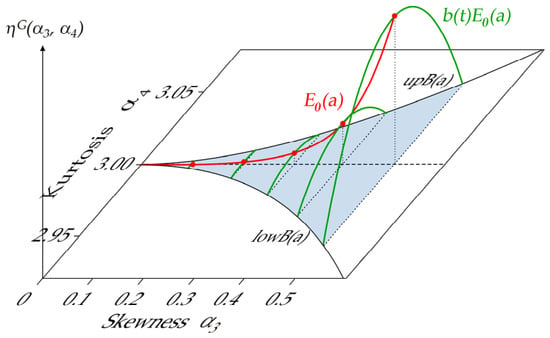
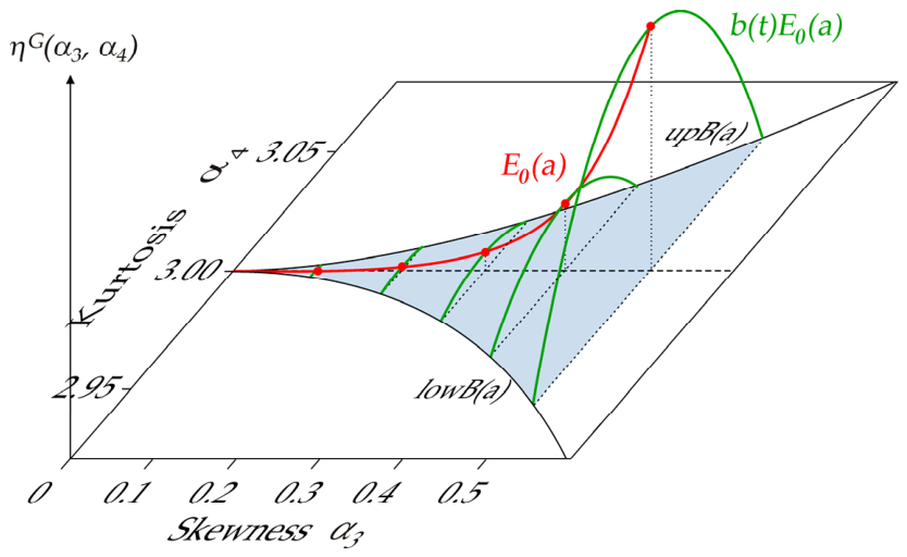
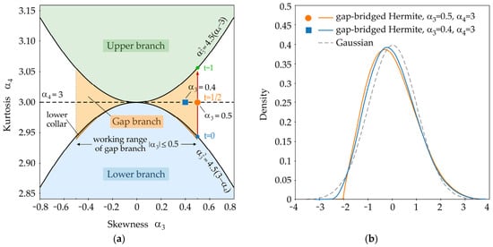
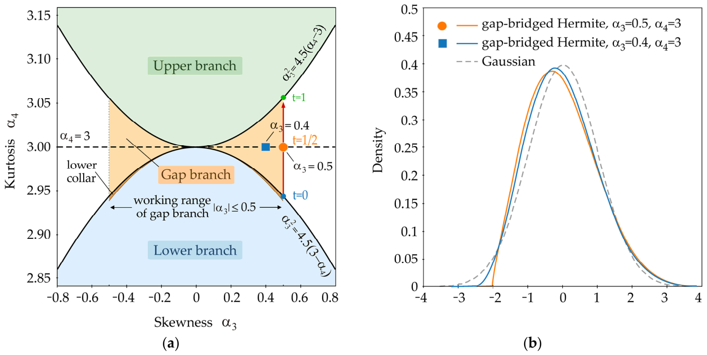
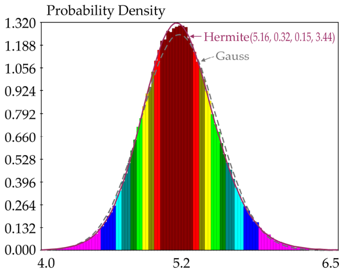
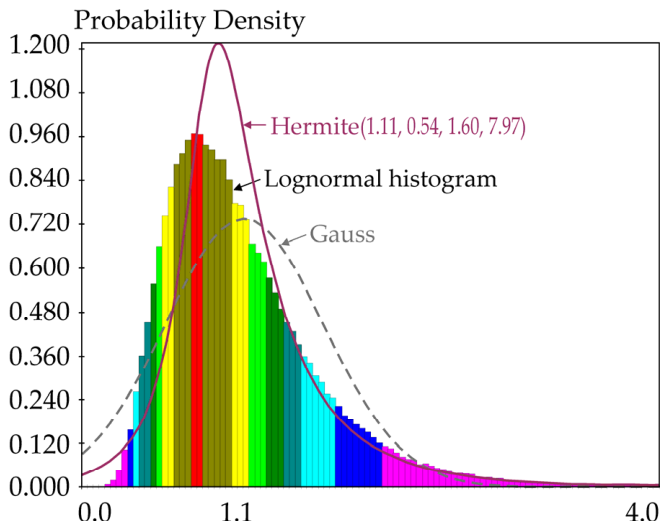
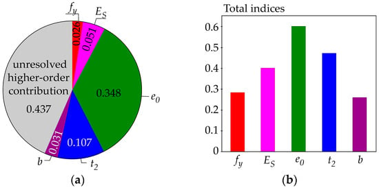
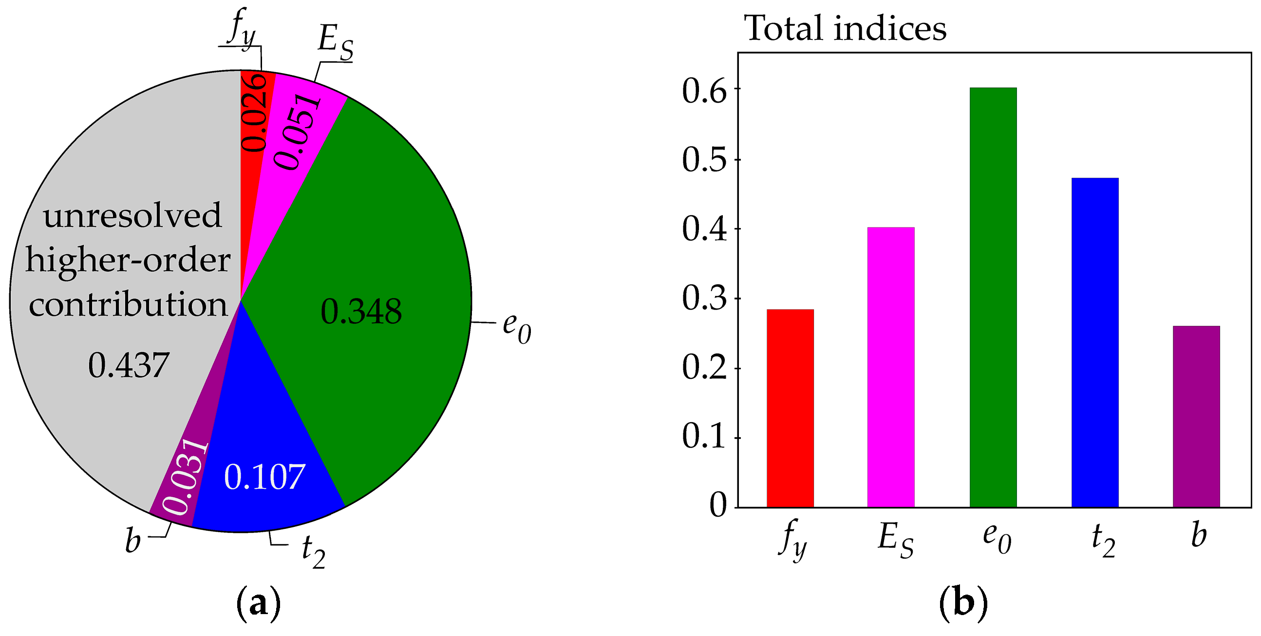
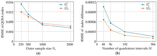
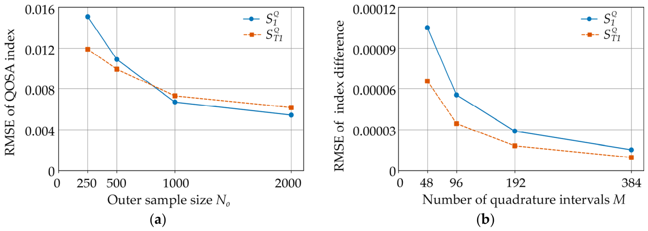

Disclaimer/Publisher’s Note: The statements, opinions and data contained in all publications are solely those of the individual author(s) and contributor(s) and not of MDPI and/or the editor(s). MDPI and/or the editor(s) disclaim responsibility for any injury to people or property resulting from any ideas, methods, instructions or products referred to in the content. |
© 2026 by the author. Licensee MDPI, Basel, Switzerland. This article is an open access article distributed under the terms and conditions of the Creative Commons Attribution (CC BY) license.