


Abstract
Quantum Annealing (QA) presents a promising approach for large-scale combinatorial optimization, though its adoption in the shipping industry remains limited. This study considers a Traveling Salesperson Problem with Time Windows and Earliness Penalties (TSPTW-EP) motivated by a break-bulk cargo-routing use case. A vessel must determine a port-visitation sequence while minimizing sailing and early-delivery storage costs and satisfying arrival-time windows. Direct Quadratic Unconstrained Binary Optimization (QUBO) formulations are limited in size by the hardware constraints of existing annealers and may suffer from rugged energy landscapes arising when encoding the continuous time variables in binary variables. Therefore, a hybrid Benders decomposition approach is proposed. The master problem, selecting port visitation sequences, is formulated as a QUBO and explored on a quantum annealer, while the classical subproblem determines arrival times and produces Benders cuts. Benchmark experiments compare different quantum and classical master solvers within the hybrid scheme on realistic maritime instances, assessing solution quality, runtime, and scalability. Results show that on the considered model, the hybrid pipeline struggles with the feasibility of QUBO solutions, especially due to the need for embeddings onto the QPU hardware. However, they also suggest that hybrid Benders terminates in fewer iterations than the classical Benders decomposition, at the cost of an uncertified stopping criterion and lower solution quality. The study aims to quantify the practical benefits and limits of QA-enabled logistics optimization.
MSC:
68Q12; 90B06; 90C11; 90C27; 90C09
1. Introduction
Shipping is the backbone of the global economy, enabling the efficient movement of goods around the world. Ensuring safe, reliable, and on-time deliveries requires the coordination of numerous complex operations in a highly dynamic environment. Many of the challenges faced by shipping companies can be formulated as large-scale combinatorial optimization problems that require fast, high-quality solutions. Exact optimization methods can provide high-quality solutions but may become computationally intractable as the number of variables increases. Consequently, practical decision-support systems often combine exact methods, heuristics, and decomposition techniques to obtain useful solutions within acceptable time limits.
Emerging optimization paradigms, such as quantum computing and quantum annealing in particular, offer promising potential to address large-scale combinatorial problems. However, applications of these technologies in the shipping industry remain limited.
This work investigates the potential of a hybrid quantum-classical optimization approach for a practically motivated break-bulk cargo-routing problem. A hybrid Benders decomposition is developed in which quantum annealing is used to generate solution candidates of the master problem containing binary routing decisions, while time-window feasibility is evaluated classically in the subproblems.
Break-bulk shipping is an essential component of global project logistics, enabling the transport of cargo that cannot be accommodated in standardized containers. This cargo includes oversized, irregularly shaped, extremely heavy, or hazardous items, for example turbines, cranes, railway vehicles, aircraft components, steel beams, bridge sections, wind-turbine blades, tanks, boilers, pipes, and industrial machinery [1]. In contrast to containerized liner shipping, break-bulk operations are typically project-driven and characterized by volatile demand, heterogeneous cargo requirements, and a limited number of recurring trade lanes.
This study is conducted in collaboration with Harren Group, a German shipping company specializing in integrated project logistics and heavy-lift transport. Its fleet ranges from mini bulkers to post-panamax vessels, with capacities between 36,000 and 92,000 deadweight tonnage. Planning voyages for such vessels requires the continuous adaptation of routing decisions to changing customer requests, port availability, contractual delivery commitments, weather conditions, bunker prices, and port costs. Because break-bulk cargo often requires specialized handling and coordination at each port call, inefficient route planning may lead to substantial fuel consumption, delays, and underutilization of vessel capacity and operational resources.
A central decision problem in this setting is the cargo routing problem: determining the sequence in which a vessel should visit a set of ports while minimizing fuel consumption and satisfying contractual obligations. In this work, we model this problem as a Traveling Salesperson Problem with Time Windows and Earliness Penalties (TSPTW-EP), an extension of the well-known TSPTW [2]. Given a depot and a set of mandatory ports, the objective is to determine a minimum-cost route that visits each port exactly once. The costs include sailing costs based on fuel consumption, and storage costs for cargo stored at the port in case of early arrivals. Each port must be serviced within a specified time window, defined by an earliest and latest admissible arrival time. These time windows may arise from berth availability, contractual delivery dates, tidal restrictions, or cargo-handling requirements and have a direct effect on storage costs. Travel times, arrival times, and possible waiting times determine whether a route is temporally feasible. Although this model represents a reduced version of the full operational planning problem, it captures the central trade-off between routing efficiency and time-dependent contractual constraints. The resulting optimization problem is combinatorial and computationally challenging. In practice, voyage plans are often adjusted manually using expert knowledge and iterative scenario analysis. While such approaches are valuable, they can become time-consuming and inflexible when operational conditions change frequently. Fully integrated optimization models can incorporate a broad range of relevant factors, but their computational complexity may prevent the rapid generation of high-quality solutions for operational decision-making.
The goal of the TSPTW-EP is to minimize fuel consumption and storage costs while respecting port time windows, contractual deadlines, and vessel capabilities. Because the problem is combinatorial and the company’s operational data are large, we propose a hybrid (quantum-classical) Benders decomposition that separates the problem into a master problem (route design) and classical subproblems (route feasibility and storage costs). The master problem is reformulated as a Quadratic Unconstrained Binary Optimization (QUBO) problem and solved on a D-Wave quantum annealer, while the subproblems remain as Linear Programs (LP) and are handled classically, giving a clear split between quantum and classical resources.
Quantum computing has emerged as a potential approach for solving difficult combinatorial optimization problems. Current quantum hardware can broadly be divided into gate-based quantum computers and quantum annealers. Gate-based devices are universal in principle but remain limited by noise, restricted qubit counts, limited connectivity, and demanding hardware requirements. Quantum annealers, in contrast, are specialized devices designed to search for low-energy solutions of Ising and QUBO models [3]. Quantum annealing is, therefore, particularly relevant for combinatorial optimization; however, real-world problems usually contain constraints that must first be encoded as penalty terms in a QUBO formulation.
This transformation creates two major challenges. First, binary encodings and penalty terms may substantially increase the number of variables and quadratic interactions in the model. Second, a logical QUBO must be embedded into the sparse hardware topology of the quantum processing unit (QPU). This embedding can require chains of physical qubits, thereby increasing physical resource requirements and affecting solution quality. Consequently, the size of problem instances that can be solved directly on current QPUs remains limited.
Many recent quantum-optimization studies, therefore, rely on hybrid solvers like the D-Wave hybrid solver that combine classical and quantum computational resources. Although this hybrid approach can address larger instances, it is not possible to attribute solution performance transparently to either the classical or quantum component. This limitation is particularly relevant when assessing the practical contribution of quantum hardware. Existing applications of quantum annealing in maritime optimization remain scarce, while related studies in other application domains often use hybrid solution frameworks because of problem-size limitations [4,5].
In addition to the decomposition approach, we describe the complete transformation from the routing model to a binary quadratic formulation. This includes the selection of binary encodings, the construction of penalty terms, and presolve techniques for reducing the model size before quantum processing. We further investigate the influence of different embedding strategies. In particular, embedding decisions affect physical qubit usage, chain lengths, and the robustness of the annealing process.
The numerical study compares three solution approaches: (i) Benders decomposition with a quantum-annealing-based master problem and classical subproblems, (ii) Benders decomposition with simulated annealing for the master problem (without and with embedding onto a sparse hardware graph), and (iii) a fully classical Benders decomposition approach. Simulated annealing provides an important benchmark because it helps distinguish potential benefits and challenges arising from quantum hardware from those attributable to a general annealing-based metaheuristic. Meanwhile, comparison to simulated annealing with embedding, as proposed in [6], reveals the bottlenecks that the need for a hardware embedding brings with it. The comparison between the master solvers evaluates not only solution quality and runtime, but also feasibility, computational-resource requirements, and the practical implications of using a standalone QPU.
For the problem sizes considered in this study, classical optimization methods remain highly competitive. Accordingly, this work does not claim a quantum advantage. Instead, it aims to establish a rigorous and transparent basis for assessing the usefulness of quantum annealing in maritime routing applications. Following recent discussions on the practical evaluation of quantum computing, such an assessment must account for hardware limitations, noise, rapidly improving classical methods, and the specific requirements of the application domain [7]. In the near term, practical value may arise not only from asymptotic speedups, but also from improved solution workflows, reduced modeling effort, or faster concept-to-solution development.
To the best of our knowledge, this study is the first to present an end-to-end quantum-annealing pipeline for a real-world shipping-industry routing use case with problem instances derived from operational data and executed on a standalone QPU. The contributions of this work are threefold:
- We introduce a practically motivated break-bulk cargo routing use case and formulate it as a TSPTW-EP that reflects key operational constraints of maritime project logistics, such as considering preferred time windows for delivery or pickup in ports.
- We develop a QPU-oriented solution pipeline that combines Benders decomposition, QUBO modeling with penalty coefficient determination via the big-M method, presolve reduction, feasibility filters and hardware-aware embedding.
- We provide a systematic comparison of quantum annealing, simulated annealing, and classical Benders decomposition, thereby establishing a transparent benchmark for evaluating quantum optimization methods in maritime decision support.
1.1. Related Works
1.1.1. TSP
The Traveling Salesperson Problem (TSP) asks for the shortest possible tour that visits each city in a given set exactly once and returns to the starting city, given pairwise distances between cities. It is a central NP-hard problem in combinatorial optimization [8]. Classical research has developed three main lines of methods. First, exact algorithms such as the Held–Karp dynamic programming approach [9] and modern branch-and-cut solvers like Concorde [10] can find optimal tours and have solved very large benchmark instances, but with exponential worst-case running time. Second, approximation algorithms provide worst-case guarantees for structured variants: Christofides’ algorithm yields a 1.5-approximation for the metric TSP [11], and polynomial-time approximation schemes for the Euclidean TSP [12] can get arbitrarily close to optimal, though they are mainly of theoretical interest. However, assuming , the general TSP cannot be efficiently approximated. Third, and most relevant for practical large-scale instances, are heuristics and metaheuristics. Local search–based methods, especially the Lin–Kernighan heuristic [13] and its advanced implementation Lin–Kernighan–Helsgaun (LKH) [14], achieve near-optimal solutions on standard benchmark sets such as TSPLIB [15] and are widely used as standards. Overall, classical methods provide very strong baselines in terms of solution quality and, in many cases, running time; any alternative paradigm, including quantum annealing, must, therefore, be evaluated relative to these well-established exact and heuristic approaches. The rise of quantum computing has motivated alternative formulations for the TSP, which are essential for execution on quantum annealers and gate-based variational algorithms [16,17], but current studies are largely exploratory and are typically benchmarked against the well-established classical methods described above.
1.1.2. TSPTW
The Traveling Salesperson Problem with Time Windows (TSPTW) extends the classical TSP by associating each customer i with a (hard) time window that specifies the earliest and latest allowable start of service. A feasible tour must visit every customer exactly once, return to the depot, and schedule arrival times so that all time-window constraints are respected. If the vehicle arrives before , it may wait until service can begin; arriving after renders the solution infeasible.
Classical exact approaches use MILP formulations with branch-and-bound or branch-and-cut, exploiting strong relaxations and time-window propagation to solve small and medium-sized instances to optimality. However, the search space grows exponentially with the number of customers and the tightness of the time windows, making large real-world instances computationally challenging.
To obtain high-quality solutions within acceptable computation times, many heuristics and metaheuristics have been proposed. Local-search-based methods adapt classical TSP moves to maintain temporal feasibility, often within frameworks such as tabu search, variable neighborhood search, or iterated local search. Simulated annealing uses random perturbations of the current solution to escape local optima and can yield competitive results on benchmark instances [18,19]. Many methods are evaluated on standardized data sets derived from the Solomon instances for vehicle routing with time windows [20].
More recently, there has been growing interest in formulating TSPTW for quantum optimization frameworks, especially in the form of quadratic unconstrained binary optimization (QUBO) or Ising models. Building on the general principles for formulating combinatorial problems as QUBO models [16], ref. [21] develops a specific QUBO formulation for the TSPTW, where both the routing choices and the satisfaction of time-window constraints are encoded via penalty terms in the objective function. Ref. [22] analyze unconstrained binary models for several TSP variants, including versions with time-related constraints, with a particular focus on penalty design and resource requirements on near-term quantum devices. The potential advantage lies in exploiting quantum effects to explore the vast solution space more effectively, possibly outperforming classical heuristics for certain structured instances. These works demonstrate that TSPTW can be embedded and experimentally tackled on current quantum annealers or variational quantum algorithms. At the same time, they highlight that experiments are still limited to relatively small instances and that, for now, classical exact and heuristic methods remain the primary reference for large-scale, practically relevant TSPTW problems.
1.1.3. Quantum Computing and Routing Problems
The application of quantum computing to routing problems has been heavily studied due to their high computational complexity and their broad applicability to real-world logistics. Within quantum computing, gate-model and annealing-based computers represent the two primary coexisting paradigms. For combinatorial optimization, including routing problems, quantum annealing is particularly relevant. The objective function can, under loose conditions, be formulated as a Quadratic Unconstrained Binary Optimization Problem (QUBO) and thus naturally mapped to a Hamiltonian encoding the problem [23]. Historically, the Traveling Salesperson Problem (TSP) and the Vehicle Routing Problem (VRP) stand out as the most widely addressed benchmarks [24]. For instance, ref. [25] proposed the first formulation of the TSP specifically tailored for a quantum annealer. Later, ref. [26] proposed a strategy for tuning parameters to solve the VRP through quantum annealing.
As the research matures, the focus shifts from canonical forms to more complex routing variants. Recently ref. [27] explored quantum annealing for the selective TSP, which introduces profit-based constraints where the objective is to maximize collected rewards within a travel budget. Significant focus has also been placed on accommodating time windows, which are one of the most frequently imposed restrictions in practical routing environments. Ref. [28] addressed the VRP with time windows using D-Wave’s Constrained Quadratic Model (CQM) solver in a hybrid framework. They observed that while the quantum solver excels at minimizing routing costs, it struggles to maintain strict time-window feasibility as the problem scales. Consequently, classical heuristic methods were applied to swap variables and fix infeasible solutions.
1.1.4. Benders
Benders decomposition is applied to mixed-integer linear programs (MILPs) where the variables separate into two groups: complicating variables (typically integer) and easy variables (typically continuous). The key idea is that if the complicating variables are fixed to a candidate value , the remaining problem in the easy variables becomes a simple linear program (LP) that is easy to solve.
Formally, consider the MILP:
where x are the complicating variables (e.g., integer) and y are the continuous easy variables. When x is fixed to , the subproblem in y is an LP:
Benders decomposition reformulates the original problem into a master problem (involving only x and an auxiliary variable representing the best subproblem cost) and the subproblem above. Solving the subproblem yields dual information (the optimal dual multipliers or an infeasibility ray). This information is used to generate Benders cuts—feasibility cuts (if the subproblem is infeasible) or optimality cuts (if it is feasible)—that are added to the master problem. Master and subproblem are solved iteratively, and the cuts progressively refine the master’s approximation until convergence to the optimal solution.
In the case of an unbounded dual subproblem, the primal subproblem is infeasible, and a feasibility cut can be generated, restricting the direction along which the dual subproblem becomes unbounded. In contrast, a feasible dual subproblem provides an actual value to a solution and, therefore, an upper limit on the overall solution value (when combined with the value of the master problem).
Since an optimal solution to the master problem gives a lower bound on the solution, and feasible solutions to the subproblem yield an upper bound on the optimal value, together these provide an optimality window in which the optimal solution value lies. The procedure terminates once the optimality gap between the exact solutions to the master and subproblem closes, at which point the primal subproblem has to be solved for the chosen values of the master solution.
The algorithm was originally proposed by Benders in [29] to decompose MILPs. Later on, the algorithm was extended by Hooker in [30] to decompose general optimization problems. This procedure is usually denoted by Logic-based Benders decomposition. For a general problem, the subproblem might not be an LP, and linear duality cannot be used. Instead, the Logic-based Benders decomposition uses logical deductions from the subproblem solution to derive cuts. This is called solving the inference dual and has to be developed for the specific type of problem.
The Benders decomposition and its variants have been successfully employed to problems in a wide variety of domains. These include the restructuring of power systems [31], the design of logistics networks [32] and the scheduling of health services for patients’ personalized care plans [33].
1.1.5. Hybrid Benders
Using Benders decomposition becomes particularly advantageous when one wants to solve the problem using quantum computing. Mapping a problem to quantum hardware usually involves transforming the problem formulation into a QUBO. Hence, every continuous variable has to be decomposed into a series of binary variables. The number of necessary binary variables depends on the chosen embedding, but in general does not scale better than logarithmically in the range and precision of the continuous variable. For MILPs, this can significantly increase the problem size, introducing additional overhead. Hence, it is of interest to decompose the continuous part from the integer part and solve it separately on classical hardware, as introduced in [34,35]. In [34], the authors use MILPs with four binary and four continuous variables as well as three constraints to test their method using quantum annealing. They also tested larger instances of the unit commitment problem, but only using simulated annealing due to the hardware limitations of the time. Similarly, in [35], the authors restrict to MILPs with two binary and four continuous variables as well as nine constraints. They also used quantum annealing for benchmarking. This kind of hybrid quantum-classical Benders decomposition approach has since been applied in multiple works. In [36], the method is applied to the design of cost-optimal multi-energy systems using quantum annealing. In [37] the authors instead map the main problem to a neutral atom quantum computer. They solve randomly generated MILPs with two to five binary and two to ten continuous variables as well as five to fourteen constraints using a quantum simulation of a neutral atom quantum computer. Conversely, ref. [38] utilizes the quantum approximate optimization algorithm (QAOA) to solve the master problem on a digital quantum computer. They test their method on MILPs with two binary and four continuous variables and nine total constraints. Finally, ref. [39] introduces methods to decouple the master problem into multiple smaller local master problems and applies these to solve the unit commitment problem using quantum annealing.
In contrast to these studies, which are mostly based on small-sized, hand-crafted or randomized MILP instances, we apply the hybrid quantum-classical Benders decomposition to medium-sized MILPs stemming from a real-world application derived in cooperation with an industry partner. We apply extensive preprocessing methods to enable benchmarking of these instances on current quantum annealing devices and include all these steps into a pipeline that paves the way for investigating the potentials of quantum computing for real-world combinatorial optimization problems.
2. Materials and Methods
2.1. Use Case and Modeling Assumptions
The use case examined in this paper was developed in collaboration with Harren Group, a shipping company from Bremen (Germany), specializing in integrated project logistics and heavy-lift transportation. The underlying operational challenge concerns a vessel-routing problem motivated by maritime cargo transportation between ports in North, Central and South America. A specialized vessel must visit a set of ports and deliver cargo while meeting customer-specific delivery requirements.
Planning such a voyage is challenging because a large number of possible port sequences (routes) have to be compared while taking numerous operational aspects (i.e., constraints) into account. To keep the model small and obtain problem instances of a manageable size for benchmarking on currently available quantum computing hardware, the real-world operational challenge is reduced to its most important aspects: The routing of a single vessel between the ports and the time-dependent delivery requirements specified by the customers. We assume a constant sailing speed for each optimization run. A real-world scenario can be simulated by discretizing and varying the allowed speed range for a ship and by solving the resulting routing problem for each speed in range.
Based on the constraints between the shipping company and its customers, there is a preferred arrival window during which the cargo can be collected immediately at the port. Arrival within this window, therefore, incurs no additional storage costs. The cargo may also be delivered during the preceding early-arrival interval . In this case, the cargo must be stored at the port until it can be collected by the customer.
The resulting storage costs are indirectly passed on to the carrier through the contracts and are assumed to increase linearly with the duration between the vessel’s arrival and the opening of the preferred arrival window. A delivery before the early-arrival interval or after the preferred arrival window, i.e., outside of , is not possible. The combined interval is referred to as the hard arrival-time window.
The planning objective is to determine the port-visitation sequence and the corresponding arrival times such that the total costs, consisting of sailing and storage costs, are minimized. Sailing costs represent fuel-related operating costs and are assumed to be proportional to sailing distance because the vessel travels at a fixed speed. Storage costs represent the costs associated with storing cargo until it can be collected by the customer. Both cost components are expressed in a common monetary unit.
The reduced problem retains the key decisions regarding the routing planning and arrival-scheduling, but disregards operational details such as multiple vessels, heterogeneous cargo, variable sailing speeds, port-capacity restrictions, and weather-dependent sailing times.
Since it is assumed that there is only one customer per port, only the term “port” is used in the following.
- Modelling assumptions TSPTW-EP
- The reduced problem consists of the following components and assumptions:
- A single vessel performing one round trip.
- A home port, which serves as a depot, where the round trip begins and ends.
- A set of ports (excluding the home port) that have to be visited exactly once.
- Sailing distances between all relevant pairs of ports are known and deterministic.
- The vessel travels at a fixed and constant sailing speed. Therefore, sailing times and the associated sailing costs (fuel consumption) are assumed to be proportional to sailing distance.
- Hard arrival-time windows for each port - arrival outside this interval is prohibited.
- A preferred, penalty-free arrival window within the hard arrival-time window (i.e., ).
- An early-arrival time window in which arrival is permitted but incurs a linear early-arrival cost proportional to the time difference between the arrival time and .
- In some ports there are no time-wise restrictions, such that a penalty-free arrival is possible at every time.
- W.l.o.g it is assumed that the earliest possible arrival time at a port is no earlier than the sailing time from the depot to that port.
- Between two ports there is always at least one location where the vessel can drop anchor and wait until the next port’s delivery window opens or until a more favorable time arrives. Waiting costs are neglected.
- W.l.o.g cargo-handling times (service times) at all ports are assumed to be zero.
Under these assumptions, the baseline problem is referred to in the following as the Traveling Salesperson Problem with Time Windows and Earliness Penalties (TSPTW-EP). An exemplary problem instance of the TSPTW-EP with its solution is presented in Figure 1.
Figure 1.
Time-window structure and example solution for one TSPTW-EP instance. The horizontal axis shows time (in hours), the vertical axis the port indices (with index 0 for the depot). While blue horizontal bars represent the early-arrival time windows at each port, the orange bars mark the preferred penalty-free time windows. Red dots are the actual arrival/service times of the vessel at the ports. Green horizontal segments between ports show traveling periods; purple segments mark an anchorage at an example location between the ports that the ship can use to arrive at the port at a convenient time. In operational practice, rather than actually anchoring, the vessel is also allowed to travel with reduced speed to arrive closer to the suggested service time.
2.2. Mathematical Formulation of the TSPTW-EP
The reduced vessel-routing problem is formulated as a Traveling Salesperson Problem with Time Windows and Earliness Penalties (TSPTW-EP). The well-known Traveling Salesperson Problem covers, in terms of graph theory, the problem of choosing a Hamiltonian cycle (i.e., a cycle in a graph visiting each node exactly once) with minimal edge weight in a graph. In our case, the nodes correspond to the ports and the edges represent valid voyages between ports with sailing costs as their edge-weight. In TSPTW-EP, the problem is extended by also taking into account arrival times at the ports, which are constrained by corresponding constraints, and storage costs for early arrivals.
The presented formulation of the model is based on the compact Mixed-Integer Linear Programming (MILP) formulation of the symmetric Traveling Salesperson Problem with Time Windows (TSPTW) presented by [40], which builds on the formulation proposed by [41]. To represent the temporal order of the voyage, the home port is modeled as separate start and end depot nodes ( resp. ). The resulting route is, therefore, a path from to that visits every port exactly once. The formulation is extended by earliness penalties to represent storage costs incurred when cargo is delivered before a customer’s preferred arrival time.
Separate parameters are used for sailing distances, sailing times and sailing costs. Since it is assumed that sailing distances between all pairs of ports are known and deterministic, the vessel travels at a fixed speed and sailing costs are proportional to sailing distances, all of them are deterministic.
| Sets and indices |
The home port is represented by separate start and end depot nodes in order to model the temporal order of the round trip without imposing time constraints around a cycle. The set of feasible sailing arcs contains all voyages between ports (s.t. the graph is complete except the direct arc between and ) and is, therefore, defined as
| Parameters |
Let denote the fixed sailing speed. Then the sailing times are given by
It is assumed that the fuel-related sailing costs are proportional to sailing distance, such that they can be expressed as
where denotes the sailing cost per unit of distance. Sailing costs and storage costs are assumed to be expressed in a common monetary unit.
| Decision variables |
Physical arrival and cargo delivery are assumed to coincide. Therefore, represents both the vessel’s physical arrival time and the cargo-delivery time at port . Due to optional waiting times while at anchor, the arrival time at a port may be later than the sum of the arrival time from the previous port and the sailing time.
Now the TSPTW-EP can be formulated as follows:
| MILP Formulation of the TSPTW-EP |
s.t. |
The big-M constant in (10) can be chosen as
s.t. the constraint holds trivially for when (9) holds. Usually, also the constraint
is needed to ensure the correct arrival times after leaving the depot, but here we assume that holds (see modeling assumptions in Section 2.1). In this case
ensures that the constraint is always fulfilled, such that it can be omitted from our model.
The objective function (4) minimizes the total sailing costs and the storage costs caused by early arrivals. The first term accounts for fuel-related sailing costs. The second term penalizes arrivals before the opening of the preferred arrival window.
For each port , the hard arrival-time window is . Arrival during the preferred arrival window incurs no storage cost. Arrival during the penalized early-arrival interval is feasible but generates an earliness value of
Because , Constraint (11) implies
Since and is minimized in the objective function, the following equality holds in every optimal solution:
Thus, the storage cost at port is given by , meaning that it increases linearly with respect to the storage time.
The arrival-travel time relation constraints permit the vessel to delay its arrival at a port, for example by waiting at sea or at the preceding port. Waiting at a port after physical arrival is not considered because physical arrival and cargo delivery coincide. Furthermore, because all sailing times are strictly positive, the arrival-travel time relation constraints eliminate subtours consisting solely of ports.
2.3. Benders Decomposition of the TSPTW-EP
The TSPTW-EP problem with a mixture of binary and continuous variables is a candidate for the Benders Decomposition (BD) as described in Section 1.1.4, which was proposed by Benders in 1962 [29].
In our case, with the TSPTW-EP, the binary routing variables are assigned to the master problem (MP) and the continuous arrival-time variables and earliness variables are assigned to the subproblem (SP). Thus, the master problem consists of finding an optimal port-visitation sequence (with minimal sailing costs), while the subproblem determines whether there exist arrival times such that this sequence can satisfy all hard arrival-time windows and, if feasible, computes the minimum early-arrival storage costs.
Therefore, the MP contains the routing constraints (5)–(8) from the MILP formulation of the TSPTW-EP and can be stated as follows.
| Master problem (MP) for the TSPTW-EP |
The variable represents the storage costs estimated by the master problem, which are also bounded from below by optimality cuts as the algorithm proceeds. Note that the MP contains no explicit constraints eliminating subtours; they are identified by the subproblem and excluded through feasibility cuts later on. In our approach, the MP is transformed into a Quadratic Unconstrained Binary Optimization (QUBO) problem and solved with quantum hardware (see Section 2.4).
For a fixed routing solution obtained from the master problem, the following linear subproblem is solved, which essentially consists of the remaining constraints from the MILP formulation of the TSPTW-EP (9)–(12).
| Subproblem (SP) for the TSPTW-EP |
If the subproblem is feasible, gives the minimum storage costs associated with the route selected by the master problem. If the subproblem is infeasible, the selected route violates at least one time window constraint. For cut generation, assume the SP is represented in the compact form
where contains the arrival-time and earliness variables resp. . Then the dual of the subproblem can be written as
Let denote an optimal dual solution for a feasible subproblem in iteration k. The corresponding Benders optimality cut is
If the subproblem is infeasible, let denote a dual extreme ray. The corresponding Benders feasibility cut is
The Benders algorithm alternates between solving the master problem and the subproblem and in each iteration the MP is extended by an additional optimality or feasibility cut. A feasible subproblem solution provides an upper bound through the combined sailing and storage costs, whereas an exactly solved master problem provides a certified lower bound. The algorithm terminates once the gap between both bounds is below a predefined tolerance (in this work a tolerance of is used).
2.4. Hybrid Optimization Pipeline
The proposed hybrid optimization pipeline combines quantum annealing for the binary master problem of the Benders Decomposition with classical optimization for preprocessing, subproblem solution, cut generation, and solution validation. In each Benders iteration, the current MP is converted into a Quadratic Unconstrained Binary Optimization (QUBO) formulation and submitted to the quantum annealer. The resulting candidate solution of the MP is evaluated classically by solving the continuous Benders subproblem.
The hybrid approach exploits the decomposition structure of the TSPTW-EP: The binary routing decisions are handled by the quantum annealer, whereas the continuous arrival-time and earliness decisions are determined classically. Benders cuts generated from the classical subproblem are incorporated into the QUBO formulation in subsequent iterations. An overview of the hybrid Benders pipeline is shown in Figure 2.
Figure 2.
Detailed flowchart of the hybrid Benders pipeline. The instance data is reduced by arc elimination (Section 2.4.1), and the initial Benders split divides the reduced MILP formulation into a master problem and a subproblem. In each iteration, the master problem is converted step by step into a QUBO: the auxiliary variable is discretized, trivial bounds are eliminated, and the remaining constraints are encoded as penalty terms whose coefficients are chosen by the Big-M method (Section 2.4.5). The QUBO is first preprocessed with roof-duality (Section 2.4.6), which fixes a part of the variables and leaves a reduced QUBO; the reduced QUBO is sampled with simulated annealing or a quantum annealer (SA or QA), the samples are filtered for feasibility, and the best candidate is passed to the classical dual subproblem, which is solved exactly with GLPK. Its optimal solution yields an upper bound (the incumbent feasible solution value), while the best feasible master candidate provides a heuristic master objective and yields a certified lower bound only if the master problem itself is solved to optimality. If the subproblem is infeasible, a dual extreme ray produces a feasibility cut. Optimality and feasibility cuts are added in the next iteration until the termination condition is fulfilled and the final feasibility check returns the solution of the original TSPTW-EP problem.
2.4.1. Preprocessing: TSPTW-EP-Specific Arc Elimination
Due to the size and connectivity limitations of current quantum hardware, it is useful to classically reduce the problem size and complexity before solving the master problem. Hence, we incorporate both a problem-specific and a simple general preprocessing step into the pipeline, which reduces the number of variables and constraints. The problem-specific preprocessing is executed a single time at the beginning of the pipeline and works as follows:
For two ports and , the arc cannot be part of a feasible route if departure from at its earliest feasible arrival time results in an arrival at after the hard deadline of port . Similar arcs from the start depot to ports can also be removed. By defining these sets of infeasible arcs as
one can now specify the reduced arc set by
In the following only this reduced set is used.
After arc elimination, the one-hot constraints (5)–(8) may imply additional variable fixings and constraint eliminations. For example, if from the start depot only the port is reachable in time, meaning for all ports , then constraint (5), i.e., , forces the remaining to be equal to 1. Consequently, this variable and constraint can be removed from the model.
Such implications are propagated iteratively until no further variable fixings can be derived. In our optimization pipeline, the above rules are executed as the first step after instance generation and before model building. This leaves us with a possibly reduced set of free routing variables , reducing the size of the master problem.
2.4.2. Conversion of the Master Problem to BIP
Throughout each iteration of Benders decomposition, the native form of the master problem, as specified in Section 2.3, is a MILP with a single continuous variable .
As a first step towards a QUBO formulation of the MP, the is now discretized by binary variables using a binary encoding of choice. Encoding decisions affect not only the size and density of the logical QUBO, but also the performance of the effective solution with QUBO solvers [42]. Although not the most straightforward to optimize due to a large dynamic range in its coefficients, for the benchmarks we opted for the logarithmic encoding, which most efficiently addresses the size constraints. To keep the number of binary variables small, in each iteration an upper bound has to be determined.
Consider an optimality cut . Note that for all x it holds
Because is minimized and it only appears in such optimality cuts, one can bound (for all optimality cuts) by
Defining and using a precision of we can finally encode by
With this substitution, the master problem is already a Binary Integer Program (BIP) with only binary variables.
2.4.3. Preprocessing: Trivial Bound Elimination
Next to the problem-specific preprocessing, a generic method for eliminating trivial bounds (cf. [43] [Section 3.1]) was integrated into the pipeline. This method is applied whenever constraints are converted to QUBO penalty terms, hence at the initial generation of the master problem and in every iteration when optimality or feasibility cuts are added. The aim is to avoid introducing unnecessary slack variables and thus keep the number of variables in the QUBO problem low.
In the following explanation we restrict to one-sided inequality constraints, as constraints of any other form, e.g., the routing one-hot constraints, will not be trivial after the problem-specific preprocessing. Notice that by flipping binary variables , any one-sided inequality constraint in a binary integer program can be written as the Knapsack constraint
where is an upper bound. In this normalized form, it is checked whether the constraint is trivial by evaluating . If this holds, the inequality (16) is satisfied by every binary assignment and can, therefore, be removed. This reduction is applied to the feasibility cuts and other inequality constraints after normalization.
2.4.4. Conversion of BIP to QUBO
After discretization of and the trivial bound elimination, the master problem consists only of binary variables. As remaining steps toward a QUBO problem, the constraints need to be addressed. For this, standard penalty term methods are employed. The equality constraints (5)–(8) can easily be transformed into quadratic penalty terms by subtracting the constant right-hand side from the constraint body and adding the square of the resulting term to the objective with an eligible penalty coefficient. For instance, for (8), we obtain the penalty term
where is the penalty coefficient of choice.
For the remaining inequality constraints, i.e., the feasibility and optimality cuts, first express them again in the normalized form (16)
The coefficients and the right-hand side u originate from the dual solution and are, therefore, generally non-integer. To obtain an integer representation without altering the cut, every coefficient and the right-hand side is first expressed as a rational number with bounded denominator. All values are then multiplied by the least common multiple L of the denominators and divided by their overall greatest common divisor G, yielding
with . Since the same positive factor multiplies both sides, the feasible set of the inequality is unchanged; no coefficient is rounded individually. The common factor is absorbed into the penalty coefficient . Appendix D reports a consistency check of the exact Benders baseline, including the cut generation, against the original MILP. By introducing a non-negative slack variable s, the corresponding penalty term is given by
Finally, the slack variable s is also represented by a binary logarithmic encoding.
2.4.5. Choice of Penalty Coefficients
The choice of penalty coefficients has a significant impact on the performance of the annealing procedure. The penalties have to be large enough such that no infeasible solution has a smaller objective value in the QUBO than the feasible optimum. However, the spectral gap, i.e., the difference of the two smallest eigenvalues of the Hamiltonian associated with the QUBO, decreases with increasing penalty [44]. A smaller spectral gap demands more precision in the annealing and thus a longer annealing time. This motivates that the penalty coefficients should be set as small as possible while still being large enough to avoid infeasible minima. Finding the smallest penalty that conserves the feasible optimum is an NP-hard problem [44], so we have to rely on heuristics.
Let be an upper bound on the objective value of a feasible solution and let be a lower bound on the unconstrained objective value. If every constraint violation induces a penalty of at least , a sufficient penalty coefficient is
Since all constraint coefficients are scaled to a common integer lattice with greatest common divisor one, every violation changes the constraint body by at least one. Hence, can be set to 1. A trivial penalty is obtained by taking U as the absolute sum of all coefficients in the quadratic cost function and . This is always big enough, since it is bigger than all values the unconstrained problem can obtain.
A more sophisticated approach is described in [44] and will be denoted as Big-M heuristics in the present work. Here, it is implemented by letting a MILP solver run on the constrained problem formulation (the BIP) for a limited time to obtain the upper bound U. We chose to use the MIP solver of the GNU Linear Programming Kit (GLPK) [45] and let it run for 1 s. For the lower bound, the SDP relaxation of the unconstrained problem is solved to optimality. For this, we use the Splitting Conic Solver [46]. Since this heuristic is quick to compute, we reevaluate the penalty after each added cut, as for a stronger constrained problem, the penalty might have to be increased.
Alternatively, the penalty coefficient can also be given as a constant beforehand, to allow for comparisons and performance increases. One might also want to give separate constant penalties for the model constraints and for the cut constraints, as violations of the cut constraints only impact the convergence, but violations of the model constraints yield infeasible solutions.
2.4.6. QUBO Preprocessing: Roof-Duality
As the last step before sampling solutions to the transformed master problem, a further presolve method is employed at the QUBO level. It is the deterministic roof-duality presolve [47], as implemented in D-Wave’s Ocean software package [48]. Based on the QUBO coefficients, the method allows for identifying lower bounds and variables which can be fixed in some (strict = False) or all (strict = True) optimal solutions. To minimize the effective size of the QUBO master and correspondingly maximize the number of fixed variables, we use it with the strict = False argument.
2.4.7. Hybrid Benders Iteration
The hybrid Benders procedure starts with the preprocessed routing model and an initial master problem without problem-specific Benders cuts. In each iteration, the current binary master problem is converted into a QUBO formulation and submitted to the quantum annealer.
The returned samples are decoded and evaluated using the original discretized binary master problem rather than their QUBO energy alone. Samples violating routing constraints or accumulated Benders cuts are discarded. Among the remaining samples, the candidate with the lowest master-problem objective value is selected.
For the selected routing solution , the continuous subproblem is solved classically to optimality using an arbitrary LP solver. For the benchmark, we used the generic GLPK solver. As described in Section 2.3, if the subproblem is infeasible, a dual ray is extracted and used to construct a Benders feasibility cut. If the subproblem is feasible, an optimal dual solution is used to construct a Benders optimality cut. The resulting cut is added to the binary master problem and is incorporated as a penalty term during the QUBO construction of the next iteration.
If, in any given iteration, no feasible candidate solution is found for the master problem, the subproblem is still solved using the candidate with the lowest QUBO energy. We deliberately continue with this infeasible sample instead of aborting the run, because in our experiments there were cases in which the algorithm was able to regain feasibility within the next two iterations. We consider this preferable to terminating the run immediately. However, if three consecutive infeasible iterations occur, the algorithm is aborted and the run is classified as failed.
Similarly, the run is considered failed if, in any iteration, the QUBO formulation of the master problem cannot be embedded on the quantum annealing hardware, either because the number of binary variables exceeds the available capacity or because no embedding is found within the time limit.
The procedure is repeated until one of the following conditions is met: either a maximum of 100 iterations is reached, or the gap between the value of the selected master solution and the storage-cost component of the incumbent feasible solution falls below 0.1 (the convergence criterion). The run is then deemed successful if a feasible solution has been found. Otherwise, it is considered failed. For the exact GLPK baseline, the test compares a certified lower bound with the value of a feasible incumbent solution and thus acts as a certified optimality-gap criterion. For the heuristic QA and SA master solvers, the sampled value is only an estimate, so the same numerical test is a heuristic stopping rule. Note that the exact GLPK baseline retains the continuous variable , whereas the QA and SA masters use the discretized encoding with resolution . The baseline, therefore, does not solve exactly the same master representation.
The resolution of the encoding also affects the stopping test. Representable values of are multiples of . Let
denote the cut-implied lower estimate at routing solution x. Any feasible discrete satisfies the cuts and is, therefore, at least . In an exact solution of the discretized master, it is the smallest such grid value and thus exceeds by less than . The computed gap is, therefore, at most smaller than the true gap implied by the continuous cuts. Consequently, the test can be satisfied while the gap of the continuous master is . Increasing to decrease the resolution (ideally to ) would make the discretized approach more closely resemble the continuous, at the cost of additional discretization variables in the master problems. In this work, we keep as a compromise, favoring smaller master QUBOs to satisfy the tight size constraints of QUBO solvers over finer discretization accuracy.
The complete procedure is summarized in Algorithm 1.
| Algorithm 1 Hybrid Benders iteration with a heuristic QUBO master solver. |
|
In summary, there are four distinct reasons for failure:
- Three consecutive master problem infeasibilities;
- Failure to find an embedding for the QUBO master problem;
- Reaching the iteration limit of 100 and not obtaining a feasible solution in the last iteration;
- The final solution being infeasible even after convergence (i.e., the stopping test was satisfied before a valid routing solution had been found).
The occurrence of these failure reasons is analyzed in Section 3.2. Because the master problem is solved by heuristic samplers (quantum or simulated annealing), the selected master objective is a heuristic master objective rather than a certified lower bound. The overall procedure, therefore, does not retain the strict lower-bound guarantee that is characteristic of exact classical Benders decomposition.
For the heuristic master solvers, this has two consequences beyond the missing lower-bound guarantee. First, the stopping test can be satisfied prematurely: whenever the sampled value is close to or above the storage-cost component of the incumbent, the test triggers even though the master problem has not been solved to optimality, and the run is reported as converged although its incumbent solution may still be suboptimal. Second, if the final master candidate violates the routing constraints while its subproblem is solvable, the test may also be satisfied before a valid routing solution has been found. Such runs are detected only by the final feasibility check and are then classified as unsuccessful. Consequently, the hybrid Benders approach with QA or SA master solvers is effectively a heuristic that terminates earlier than exact Benders decomposition, at the cost of lower and uncertified solution quality, and it may even yield an infeasible final solution. Section 3 quantifies this effect for the benchmark runs.
3. Results
3.1. Overview
For the benchmarks, we generated 132 realistic instances with different seeds and various parameter choices. In particular, we varied the number of ports n from 3 to 13, the ratio of customers without time windows from 0.1 to 0.3 and set 3 different values for the sailing speed as a scaling of travel/sailing times. For a more detailed description of the instance generation, we refer to Appendix C. In Figure 3 an overview of the problem sizes of the benchmark instances is presented, as well as the effect of the preprocessing described in Section 2.4.1.
Figure 3.
Number of initial binary variables () for all benchmark instances before and after preprocessing.
The initial number of binary variables is fixed for each n and scales quadratically. Notice, however, that the number of variables fixed by the preprocessing differs for each instance. In general, instances with tighter or less overlapping time windows profit more from the preprocessing.
To understand the properties of the QUBOs that the hybrid Benders approach produces in the iterations, we showcase information about their sizes and connectivity in Figure 4. The sizes on the x-axis are the number of free variables that remain after presolving with the roof-duality, and for the connectivity we plot the mean number of neighbors that each variable is connected to. The main problems that these QUBOs correspond to are from our first benchmark round where solver parameters were kept default (cf. Table A1) and only the employment of the preprocessing was varied. Specifically depicted is information about the main problems from hybrid runs with solver “QA” (Quantum Annealing on the Advantage QPU with heuristic minor embedding). Clearly, with increasing problem size, both the number of variables and the connectivity increase in a predictable manner, if one considers the main problems of the first Benders iterations. For the later iterations, we obtain outliers with higher connectivity due to added cuts represented by inequality constraints. This tells us that in later iterations, the main problems cast as QUBOs get harder to solve or at least require larger embeddings.
Figure 4.
Visualization of sizes (number of free variables after application of roof-duality) and mean number of connections per variable of main problems cast as QUBOs for the hybrid Benders runs with Quantum Annealing in the first benchmark round. Both active and deactivated preprocessing is considered.
Throughout the benchmarks, we ran the hybrid Benders pipeline on a common set of problem instances while varying the preprocessing, the master problem solvers, and their parameters. In particular, we employed an exact MIP solver as well as quantum annealing and simulated annealing as QUBO solvers, the latter two with different embedding methods and target hardware graphs. In the following, we refer to the master problem solvers by the abbreviations listed in Table 1.
Table 1.
Master Problem solver abbreviations and properties.
Clique embeddings [49] are precomputed and can represent fully connected QUBOs of a given size. They feature homogeneous chain lengths and are heavily limited in the QUBO size they can represent. As an alternative method, we compute embeddings with D-Wave’s minorminer heuristic [50,51], which comes with some classical overhead but ideally provides embeddings with shorter chain lengths for sufficiently sparse QUBOs. For a study of the embeddings used in the benchmarks, we refer to Section 3.3.
The master solver parameters that have been varied include the annealing time, the number of sweeps (only for SA solvers) and the chain strengths of solvers using embeddings. The annealing time is the time that a single quantum annealing run takes to transform the Hamiltonian landscape to match the QUBO problem. It is advisable to optimize for different problem sizes [52]. The analogous parameter for SA is the number of sweeps, which determines the size of the incremental steps in which the system is “cooled down”. The chain strength determines the size of penalties for chain breaks in the physical (embedded) QUBO. Low chain strengths can thus lead to many chain breaks, while high chain strengths can obscure the energy landscape similar to high penalty coefficient values [44].
An overview of the master problem solvers, the parameters varied for each of them, and their default values is shown in Table A1, while the number of runs per solver and parameter value is shown in Figure A1.
Information about the hardware that the classical side of the benchmarks ran on is provided in Appendix E.
3.2. Default Parameters: End-to-End Convergence and Solution Quality
As a first view of the benchmark outcomes, we turn to Figure 5, which shows the instance-level success rate per solver and problem size for the default parameters. Some solver–instance combinations were computed multiple times with identical default parameters. The heatmap first averages the repeated runs of each instance and then averages over instances, so every instance contributes equally. We define a run as successful if the Benders pipeline terminates with a solution that passes the final feasibility check. For the heuristic master solvers, termination is decided by the heuristic stopping criterion of Section 2.4.7, not by a certified optimality gap.Possible failure reasons have been discussed near the end of Section 2.4.7. Note that failure due to the iteration limit only applies to the exact GLPK solver (cf. Figure 6), which, by its convergence guarantee, cannot fail due to any other reason. As expected for the exact solver, i.e., the conventional Benders pipeline, it achieves the highest success rate across all instance sizes and only reaches the iteration limit for large n. The second-highest success rates are achieved by the simulated annealing QUBO solver without embedding overhead. All other solvers already struggle for much smaller problem sizes, dropping to single-digit success percentages from onward. This suggests that the need for an embedding constitutes a major bottleneck.
Figure 5.
Instance-level success rate with default parameters per master problem solver and instance size n. Each instance contributes equally: the success fraction is computed per instance over its repeated runs and then averaged over instances. Cell text: success rate and standard error over instances (omitted at zero). The x-axis tick labels give n and the number of instances.
Figure 6.
Reasons for the unsuccessful (non-success) runs per solver: stacked bars split into failure reasons, annotated with the number of failed runs per reason; labels above each bar show failed/total runs.
The failure reasons of the Benders pipeline per solver are depicted in Figure 6. Again, this considers runs with the default parameters. Due to slight asymmetries in the repeated runs across solvers, this is not a perfectly fair per-solver comparison, but it nevertheless provides an overview of the underlying challenges. For the QUBO solvers, especially the ones with embedding, the dominant issue is the repeated failure to find a feasible master solution. Out of interest, we have split this category into the runs that failed due to this at the start vs. in later iterations. In most cases, this already occurs in the first iteration, with the exception of the SA solver. This motivates our hypothesis that, for the considered optimization problem, embeddings severely reduce the chances of finding feasible solutions, which likely contributes to the low observed success rates. The occurrence of the embedding failures depends heavily on the considered problem size. Note that they occur strictly upstream of any master-problem infeasibility and, therefore, mask its full extent: a run that aborts because its master problem cannot be embedded never reaches the iterations in which consecutive infeasibilities would arise. Even without such errors, a considerable share of these runs would still be expected to fail due to repeated infeasible master problems, so the infeasibility counts shown here should be read as a lower bound. It can be seen that with the clique embedding, the Advantage2 hardware fails more often due to an embedding error than the Advantage hardware. Interestingly, for the minorminer embedding, this behavior is reversed. This is attributable to the reduced qubit count but increased connectivity of the Advantage2 system. We discuss this in more detail in Section 3.3.
The scarcity of successful runs for solvers with embedding impedes an evaluation against stricter metrics. Nevertheless, we can still examine the optimality gaps of successful runs for small problem sizes. Again, we restrict ourselves to the default parameters (see Table A1), which have been benchmarked for most solvers. Figure 7a shows the median optimality gaps of successful runs with quantum annealing (excluding the solvers with hardware in Europe (Advantage2_system2)). For these successful runs, the objective values lie close to the optimum, confirming that the hybrid Benders approach works in principle. Note that the data becomes very sparse for medium problem sizes n.
Figure 7.
Median optimality gap vs problem size n for the QUBO solvers at default parameters (final objective relative to the exact MILP solution). Each instance contributes equally: repeated runs of an instance are first reduced to their median, and the band is the interquartile range across instances. Only successful runs have a gap; hence, a survivor bias is possible for large n. Solvers are dodged horizontally so overlapping points stay visible. (a) Quantum annealing solvers. (b) SA solvers.
The analogous plot for the simulated annealing solvers is shown in Figure 7b. The trend continues: the gaps remain (near-)optimal until the success rate drops significantly, after which the optimality gaps increase slightly.
Note that converged regular Benders runs, i.e., those using the exact solver, reproduce the optimum exactly. Only three feasible results did not converge. All of them were cut off at the 100-iteration limit and are, therefore, excluded from the plots.
As a final analysis of the end-to-end results, we compare some basic properties of the hybrid Benders approach with those of exact Benders. For this, we restrict ourselves to simulated annealing without embedding as an idealized solver, for which enough successful runs were recorded to allow for a fair comparison without survivor bias. We examine the number of iterations until convergence and the total runtimes. The reported total solver time is the sum of the master and subproblem solve times over all Benders iterations. For the QUBO solvers, the master time includes QUBO conversion, embedding (where used), sampling and communication, and sample filtering/postprocessing. For the GLPK baseline, it includes the exact master solve. Penalty determination, instance preprocessing, cut generation, and the final solution assembly are excluded. Figure 8a shows the median number of iterations for the SA and GLPK solvers on instances that were solved successfully by both. As motivated by [53], the suboptimal master solutions allow the algorithm to terminate in significantly fewer iterations for sufficiently large problem sizes. However, this reduction is partly an artifact of the uncertified stopping criterion. The lower iteration count, therefore, does not demonstrate faster convergence at comparable accuracy. Restricting the comparison to equal final accuracy, i.e., to the 48 of the 92 paired instances on which the SA solver also terminates at the optimal objective value (the exact GLPK baseline is optimal on 91 of the 92 paired instances), both solvers require a median of four Benders iterations. SA needs fewer iterations on 13 of these 48 instances, the same number on 32, and more on 3.
Figure 8.
Number of iterations until convergence and solve times per instance, SA (y) vs exact GLPK baseline (x). Only instances where both solvers succeeded are shown (identical instance set on both axes). Color = n, dashed line = equal iterations; repeated runs per instance: median. (a) Number of Benders iterations until termination. Failed runs are excluded because they stop at the abort limit rather than at convergence. (b) Sum of master and subproblem solve times, log-log axes.
For the SA solver, however, this apparent advantage does not translate into an advantage in total runtime, as shown in Figure 8b. A single SA master solve costs roughly two seconds and grows with the master size, whereas GLPK completes an entire master-plus-subproblem iteration in less than a tenth of a second, leaving SA an order of magnitude slower. Additionally, the runtime of SA QUBO solves increases with the QUBO size. Since the master problem grows within a run through added cuts, this introduces an additional overhead for the SA solver, mitigating the benefit from the reduced iteration count. The runtime of quantum annealing solvers per iteration, on the other hand, increases only indirectly through embedding-related and post-processing overhead. Indeed, for the clique solvers it remains roughly constant. Hence, with more stability, the total runtime of these solvers could benefit from reduced iteration counts.
3.3. Embedding-Related Evaluation
As mentioned above, the QUBOs of the master problems in the hybrid Benders runs require an embedding onto the annealing hardware when quantum annealing is used. Table 1 lists the embedding methods and hardware architectures not only for the quantum annealing solvers, but also for the simulated annealing variants that include an embedding overhead. In particular, we compare embeddings generated by the minorminer heuristic within a two-second timeout per QUBO with precomputed clique embeddings, which support arbitrary connectivity up to a limit determined by the hardware topology. For the Advantage architecture, this limit is a QUBO size of 177, whereas for Advantage2 it is 104 due to its reduced qubit count. Note that while the heuristic incurs a classical time overhead for every QUBO, the clique embeddings do not. As a trade-off, the latter generally yield longer chains, as they are designed for fully connected problems. Reusing embeddings is not possible because the QUBO structure changes unpredictably due to the added cuts.
Figure 9 shows the average chain length of the embeddings used by the different quantum samplers for different QUBO sizes in the benchmarks with default parameters. The samplers “QA” and “QA2” correspond to the default DWaveSampler with an AutoEmbeddingComposite wrapper, i.e., local embedding search with the minorminer heuristic [50,51] on the Advantage and Advantage2 systems, respectively. The samplers “clique” and “clique2” correspondingly denote the DWaveCliqueSampler on the analogous hardware. Note that the clique embedding reaches its limit earlier on Advantage2, since for larger QUBOs the higher qubit count of the Advantage system outweighs the larger number of couplers per qubit on Advantage2. For the heuristic embedding search, the higher coupler-per-qubit count is advantageous in this regime of relatively sparse QUBOs (recall Figure 4). This not only explains the increased number of failures due to QUBO size for the clique2 solver in Figure 6, but also accounts for the slightly superior performance of the QA2 solver on the instances for which embeddings were found (cf. Figure 7a. Given the analogous embedding sizes of the corresponding simulated annealing runs, however, this does not explain the differences in solver performance depicted in Figure 7b.
Figure 9.
Mean chain lengths of the embeddings used by the quantum samplers as a function of the QUBO size in the default parameter benchmarks.
Figure 10a illustrates the influence of the embedding choice. In general, longer chains do lead to a higher probability of chain breaks during individual annealing runs. However, these do not necessarily lead to worse results, since chain breaks are repaired in post-processing by a simple majority vote.
Figure 10.
Solver metrics averaged over samples of QUBO master solves with default parameters. (a) Mean chain break fraction vs mean chain lengths of embeddings. (b) Number of feasible samples vs mean chain break fraction.
Figure 10b shows the consequences for the feasibility of individual master problem solves. Plotted are the number of feasible samples (out of 1000) and the associated mean chain break fraction per run. There appears to be a negative correlation: for a fixed solver, the feasibility rate drops significantly beyond a certain chain break fraction. Above roughly broken chains, the number of feasible samples decreases for all solvers. Interestingly, despite the clique solver using some of the largest embeddings, it produces the runs with the highest feasibility rates. Although not shown here, another interesting observation is that, for runs with feasible samples, the best QUBO objective shows no clear correlation with the number of chain breaks.
3.4. Parameter Study for the Hybrid Benders Approach
In the benchmark study, we varied several solver-related hyperparameters to see whether the default results can be improved. In particular, for quantum annealing we varied the annealing time and the relative chain strength, which is the ratio of the absolute chain strength to the largest QUBO coefficient. For simulated annealing, we varied the number of sweeps (the analog of the quantum annealing time), together with the relative chain strength for the embedded variants. For details, including the ranges of the varied parameters, see Figure A1 and Table A1. We first consider the SA solver, i.e., simulated annealing without embedding, for which only the number of sweeps was varied. Figure 11 plots statistics on the first-iteration master problem feasibility and the end-to-end optimality gap (of successful runs) for different numbers of sweeps. Both the feasibility per QUBO solve and the overall performance improve clearly with an increasing number of sweeps. This comes at the cost of a longer runtime, which scales linearly with the number of sweeps.
Figure 11.
Some results of varying the number of sweeps (different colors) of the SA solver per problem size n. Band = interquartile range across instances. (left) Median number of feasible samples in first iteration master problems. (right) Median optimality gap of hybrid Benders pipeline, only considering successful runs.
Next, we turn to the simulated annealing solvers with embeddings, for which the relative chain strength was varied as well. A relative chain strength of zero denotes the default chain strength argument of the corresponding solver. Since a hyperparameter analysis will likely depend on the problem size and hardware, it needs to be conducted for a fixed problem size and hardware combination. For clarity, we present the SA_clique and SA_search2 results for as a qualitative representative extract. The remaining results are discussed in the text. Figure 12 shows the mean chain break fraction and first-iteration feasibility rates, as well as the success rates, for these solvers. Several observations can be made. As expected, chain breaks vanish for sufficiently high chain strengths, and the default value is sufficiently high (cf. Figure 12a,b). However, only for the minorminer embedding do the chain breaks also appear to depend on the number of sweeps (Figure 12b). Interestingly, looking at the feasibility (Figure 12c,d), the optimal chain strength is not necessarily the smallest value at which chain breaks vanish. Instead, a regime in which a few chain breaks still occur seems preferable. This may balance the drawbacks of frequent chain breaks against those of large physical QUBO coefficients. For the clique solver (Figure 12c), we again observe the trend that increasing the number of sweeps improves the feasibility rates. This behavior, however, carries over neither to the minorminer embedding (Figure 12d) nor to the success rates (Figure 12e,f). Especially in panel Figure 12e, the optima are largely disjoint. This suggests that chain breaks are not the only relevant factor, and that there is no direct correlation between the first-iteration QUBO feasibility rate and the overall success rate. The reason is likely that failure depends not only on first-iteration feasibility, but also on the feasibility of later iterations. As the QUBOs grow in size and density with each iteration, the parameters that are optimal for QUBO feasibility may change from one iteration to the next. Hence, the parameters that maximize overall success need not coincide with those that maximize first-iteration feasibility. This suggests that optimizing the parameters separately for each iteration could be beneficial, which, however, is beyond the scope of this paper. While the patterns found here generally repeat for the other target graphs, i.e., the SA_clique2 and SA_search solvers, and problem sizes (except that, for , decreasing the number of sweeps increases the chain break rates for the clique embeddings), the optimal values themselves are not consistent but depend on the solver and the problem size.
Figure 12.
Some results of varying the number of sweeps and the relative chain strength of the SA_clique and SA_search2 solvers, extracted for . (a) SA_clique: mean chain break fraction in first iteration master problems. (b) SA_search2: mean chain break fraction in first iteration master problems. (c) SA_clique: mean number of feasible samples in first iteration master problems. (d) SA_search2: mean number of feasible samples in first iteration master problems. (e) SA_clique: mean success rate. (f) SA_search2: mean success rate. This is not quantitatively representative for all problem sizes n, as the optimal parameter values differ per problem size and solver. Unbenchmarked parameter combinations are excluded.
Next, we examine the analogous results for the corresponding quantum solvers in Figure 13, this time varying the annealing time instead of the number of sweeps. The chain break fractions (Figure 13a,b) behave similarly, except that the default chain strength for the clique embedding in Figure 13a allows some chain breaks. Again, however, panel Figure 13c shows that some chain breaks should be allowed to remain in order to optimize QUBO feasibility. This differs slightly for the minorminer embedding in panel Figure 13d, where a relative chain strength of yields the best feasibility results while also reducing chain break rates. The trend that metric optima do not align with global success rates repeats here, with multiple disjoint optima for the Benders success rate. As above, we suspect that this is because the optimal parameters for the QUBO master solves depend on the iteration, which entails different QUBO sizes and densities than in the first iteration. Given our earlier finding that low first-iteration feasibility is the dominant failure reason, hyperparameter optimization with constant parameters may merely shift this bottleneck to later iterations. The significant changes in success rates in panels Figure 13e,f nevertheless show that hyperparameter optimization can improve performance, although the resulting optima do not generalize well across solvers and problem sizes. As stated above, using distinct parameters per iteration, rather than a single constant annealing time and chain strength, may be beneficial.
Figure 13.
Some results of varying the annealing time and the relative chain strength of the clique and QA2 solvers, extracted for . (a) clique: mean chain break fraction in first-iteration master problems. (b) QA2: mean chain break fraction in first-iteration master problems. (c) clique: mean number of feasible samples in first-iteration master problems. (d) QA2: mean number of feasible samples in first iteration master problems. (e) clique: mean success rate. (f) QA2: mean success rate. This is not quantitatively representative for all problem sizes n, as the optimal parameter values differ per problem size and solver. Unbenchmarked parameter combinations are excluded.
3.5. Summary
Compared with the QUBO master problem solvers, the exact Benders baseline (GLPK) converges most reliably. Among the QUBO solvers, SA without embedding yields the best performance, as expected, and can even terminate after fewer iterations (though not in less time, due to computational overheads) than exact Benders. However, this earlier termination is not certified and coincides with lower solution quality. Once an embedding is required, however, the success probability of the QUBO solvers drops significantly already for small to medium instances (). When the hybrid pipeline terminates successfully, the median objective is near-optimal, but a non-negligible fraction of the runs is substantially suboptimal (cf. the optimality gaps in Figure 7). Therefore, the bottleneck is not only reliability, but also the uncertified stopping criterion. The dominant failure mode for QUBO solvers is the repeated failure to find a feasible master solution, with embedded solvers often already struggling with first-iteration feasibility. As QUBO sizes and densities grow in every iteration due to the added feasibility and optimality cuts, embedding failures also contribute. Our analysis of embeddings, chain breaks, and solver parameter sweeps shows that longer chains break more often and that QUBO feasibility collapses above chain breaks, while the feasibility optimum occurs where a few chain breaks remain. Hence, neither minimizing chain breaks nor maximizing first-iteration feasibility is the right tuning objective. In the parameter sweeps, the first-iteration feasibility maps have clear optima, but these do not carry over to end-to-end success: the success optima are disjoint and shift with solver and problem size n. Constant-parameter tuning may simply shift the infeasibility bottleneck to later iterations. Per-iteration schedules are a natural next step. The embedding comparison shows that clique embeddings reach their size limit much earlier on the Advantage2 hardware (104 vs. 177), whereas minorminer embeddings benefit from its higher connectivity. Despite the longest chains, however, the clique solver achieves the highest feasibility rates (aided by majority-vote chain repair).
4. Conclusions and Outlook
In this study, we have presented the first end-to-end hybrid quantum-classical Benders decomposition pipeline for a real-world break-bulk cargo routing problem, executed on a standalone QPU. Our work directly addresses the practical challenges of applying quantum annealing to operational maritime logistics, a domain where such techniques have until now seen little attention. It provides a framework that enables the maritime domain to investigate the potential of quantum computing when confronting similar cargo routing problems.
The study makes three core contributions.
- First, we formulated a practically motivated TSPTW with earliness penalties (TSPTW-EP) that reflects key operational constraints of break-bulk shipping, including port time windows and storage costs.
- Second, we developed a QPU-oriented solution pipeline that combines Benders decomposition with a QUBO-based master problem, classical subproblems, preprocessing, trivial bound elimination for the cuts, dynamic ranges for the real variables, and roof-duality for further QUBO reduction. In addition, the Big-M heuristic was applied to obtain sufficiently large penalty coefficients. The results show that the pipeline works as intended.
- Third, we conducted a systematic comparison of quantum annealing, simulated annealing (with and without embedding), and fully classical Benders decomposition, establishing a transparent benchmark for evaluating quantum optimization methods in maritime decision support.
Our experimental results confirm that the pipeline works as intended: the decomposition effectively separates the inherently discrete routing decisions from the continuous timing and cost evaluation, and the quantum-annealed master problem, despite being heuristic, can lead to feasible solutions. However, classical Benders decomposition remains the most reliable approach for the instance sizes considered. While the hybrid approach occasionally terminates after fewer Benders iterations than the classical method, this earlier termination relies on an uncertified stopping criterion and comes at the cost of lower solution quality. Moreover, the total runtime is not competitive due to per-iteration computational overheads. This reinforces our initial assertion that we claim no quantum advantage in this setting.
The main obstacles to practical quantum deployment are not only the limited number of qubits but also the need to embed the logical QUBO onto the sparse hardware graph. Our comparison with simulated annealing indicates that embedding is a major source of infeasibility and performance degradation. Because the embedded-SA variants use the same embeddings and postprocessing but replace the QPU with a classical SA sampler, this comparison provides evidence for a substantial embedding penalty. It does not, however, independently quantify the contribution of quantum noise, so attributing the remaining degradation to embedding alone would require a separate noise-controlled experiment. Nevertheless, we observed that tuning parameters such as chain strength and annealing time can mitigate chain breaks and improve feasibility, albeit with constant parameters that improve only individual iterations and not the end-to-end optimization across iterations. Whether a more elaborate hyperparameter optimization is worthwhile remains an open question for future research.
The present study has several limitations that must be acknowledged. First, the problem instances are deliberately small (up to 13 ports) to permit execution on current QPUs; at this scale, state-of-the-art classical solvers remain clearly superior in both speed and reliability. Second, while the distance matrices and travel times are directly derived from operational data, the instances are synthetic in the sense that they do not yet cover full real-world dynamic replanning scenarios. Third, the classical baseline is not a highly tuned commercial solver but a straightforward implementation of Benders decomposition (using GLPK), which means our classical comparison is conservative rather than state-of-the-art. Fourth, due to the abort criterion after three consecutive infeasible master iterations, we obtain censored statistics on failure modes; we partially address this by also reporting first-iteration feasibility results. Finally, the need to find an embedding and set appropriate chain strengths introduces additional manual and computational effort that is problem-specific and not yet fully automated.
These findings have important implications for future research. The demonstrated pipeline provides a reusable framework for deploying quantum annealers on real optimization problems, even when the master problem is too large for direct QPU embedding. To move closer to practical quantum advantage, future work should focus on more efficient encoding schemes, dynamic embedding strategies, and adaptive parameter selection that accounts for the changing QUBO structure across Benders iterations. Additionally, extending the model to incorporate dynamic replanning, multiple vessels, and port-specific operational constraints will increase its industrial applicability.
In closing, this study establishes a rigorous and transparent baseline for assessing quantum annealing in shipping logistics. While current quantum hardware does not outperform classical methods, the pipeline offers a structured approach that can be directly adapted as hardware matures. By clearly quantifying the bottlenecks, we provide practitioners and researchers with a clear roadmap for what is required for quantum computing to become a genuine asset in maritime decision support.
As an outlook, we encourage further research on hybrid Benders approaches for similar or different optimization problems. To make the use case more realistic and easier to adopt, one could consider multiple vessels and cargo parcels, pickups and deliveries, speed optimization, port and fuel costs, and more. Since the pipeline is generic, adapting it to different models would be straightforward. On the technical side, we see potential in optimizing the solver parameters based on the current master problem size rather than only the initial problem size. Instead of the grid search used here, more elaborate hyperparameter optimization methods such as Bayesian search could prove beneficial. Furthermore, alternative Benders variants could be integrated into the pipeline, e.g., accelerated Benders, where multiple samples of the master problem solution can be considered at once. To further reduce the complexity that the cuts add to the QUBO, additional exact or approximate reduction methods could be implemented. Similarly, different encodings of the real variable in cuts could be compared in benchmarks. Future work could consider other quantum or quantum-inspired master solvers, potentially including gate-based optimization algorithms. Another option is to replace the QUBO master with a higher-order binary optimization (HUBO) formulation, which can approximate some constraints without the slack variables required by the quadratic penalty approach [22]. For current quantum annealers, higher-order terms must be reduced to QUBO via ancilla variables, so this is unlikely to reduce the embedding burden. Native HUBO solvers, including quantum-inspired ones, could, however, be benchmarked with the same pipeline. For solvers that require an embedding, the understanding of feasibility collapse could be improved, perhaps by introducing alternative embedding methods, e.g., reusing precomputed embeddings [53].
The negative outcome may also be partly problem-specific. The TSPTW-EP combines routing with hard time-window constraints, so the subproblem can be infeasible and the master problem accumulates both feasibility and optimality cuts, each requiring slack variables. Hybrid Benders may be more promising for MILPs whose subproblems remain feasible for every master assignment. For example, in the transmission network expansion planning problem studied in [53], load shedding guarantees subproblem feasibility and, therefore, only optimality cuts are generated, and the authors report BD-QA solutions within 5% of the optimum up to eight buses. A systematic comparison across problem classes is left for future work.
Although we found no clear evidence for an advantage of hybrid Benders over conventional Benders decomposition in our operational use case, we consider it a relevant research topic, especially in light of the rapidly evolving quantum hardware landscape.
Author Contributions
Conceptualization, O.S., J.D., H.H., J.T.G. and A.R.; Methodology, O.S., J.D., H.H. and J.T.G.; Software, O.S., J.D., H.H. and J.T.G.; Validation, O.S., J.D. and H.H.; Formal analysis, O.S., J.D. and H.H.; Investigation, O.S., J.D. and H.H.; Resources, O.S. and A.R.; Data curation, O.S., J.D., H.H. and J.T.G.; Writing—original draft, O.S., J.D., H.H., J.T.G. and A.R.; Writing—review and editing, O.S., J.D. and A.R.; Visualization, O.S., J.D. and J.T.G.; Supervision, O.S., J.D. and A.R.; Project administration, A.R.; Funding acquisition, A.R. All authors have read and agreed to the published version of the manuscript.
Funding
This research was funded by the Free and Hanseatic City of Hamburg, represented by the Authority for Science, Research, Equality and Districts, under grant number E42511-04 (project “Quantum Computing for Shipping and Maritime Logistics in Hamburg” (QSH)) [54].
Data Availability Statement
The original contributions presented in this study are included in the article. Further inquiries can be directed to the corresponding authors.
Acknowledgments
We are grateful to Thomas Joachim Friese for assisting with the literature research, development and evaluation. Special thanks go to the shipping company Harren Group and especially Nils Aden, who provided us with data and crucial background information on the use case. The authors gratefully acknowledge the Jülich Supercomputing Center (https://www.fz-juelich.de/jsc (accessed on 1 April 2026)) for funding this project by providing computing time on the D-Wave Advantage™ System JUPSI through the Jülich UNified Infrastructure for Quantum computing (JUNIQ). During the preparation of this manuscript/study, the authors used DeepSeek-4.1-flash for the purposes of improving text, generating graphics and data analysis. The authors have reviewed and edited the output and take full responsibility for the content of this publication.
Conflicts of Interest
The authors declare no conflict of interest.
Abbreviations
The following abbreviations are used in this manuscript. For the master solver abbreviations, we refer to Table 1 and Appendix A. 1 if not directly referencing the corresponding solver from Table 1.
| BD | Benders Decomposition |
| MP | Master problem |
| SP | Subproblem |
| TSP | Traveling Salesperson Problem |
| TSPTW | Traveling Salesperson Problem with Time Windows |
| TSPTW-EP | Traveling Salesperson Problem with Time Windows and Earliness Penalties |
| QA 1 | Quantum Annealing |
| SA 1 | Simulated Annealing |
| QUBO | Quadratic Unconstrained Binary Optimization |
| HUBO | Higher Order Unconstrained Binary Optimization |
| CQM | Constrained Quadratic Model |
| LP | Linear Program |
| MIP | Mixed Integer Program |
| MILP | Mixed Integer Linear Program |
| BIP | Binary Integer Program |
| QPU | Quantum Processing Unit |
Appendix A. Additional Benchmark Information
Table A1.
Master problem solver configurations of the benchmark: parameters varied during the benchmarks with their ranges and defaults (defaults are used whenever a parameter is not varied). All heuristic solvers use 1000 reads per master-problem solve.
Figure A1.
Benchmark coverage: number of runs per (solver, parameter value) for the main sweep parameters. Cell text = run count, color = log10 run count. Shows which parameter values were benchmarked for which solver and where coverage is thin. Number values for relative_chain_strength represent a custom chain strength relative to the largest QUBO coefficient being employed for the embeddings, while None marks the use of D-Wave’s default argument for chain_strength.
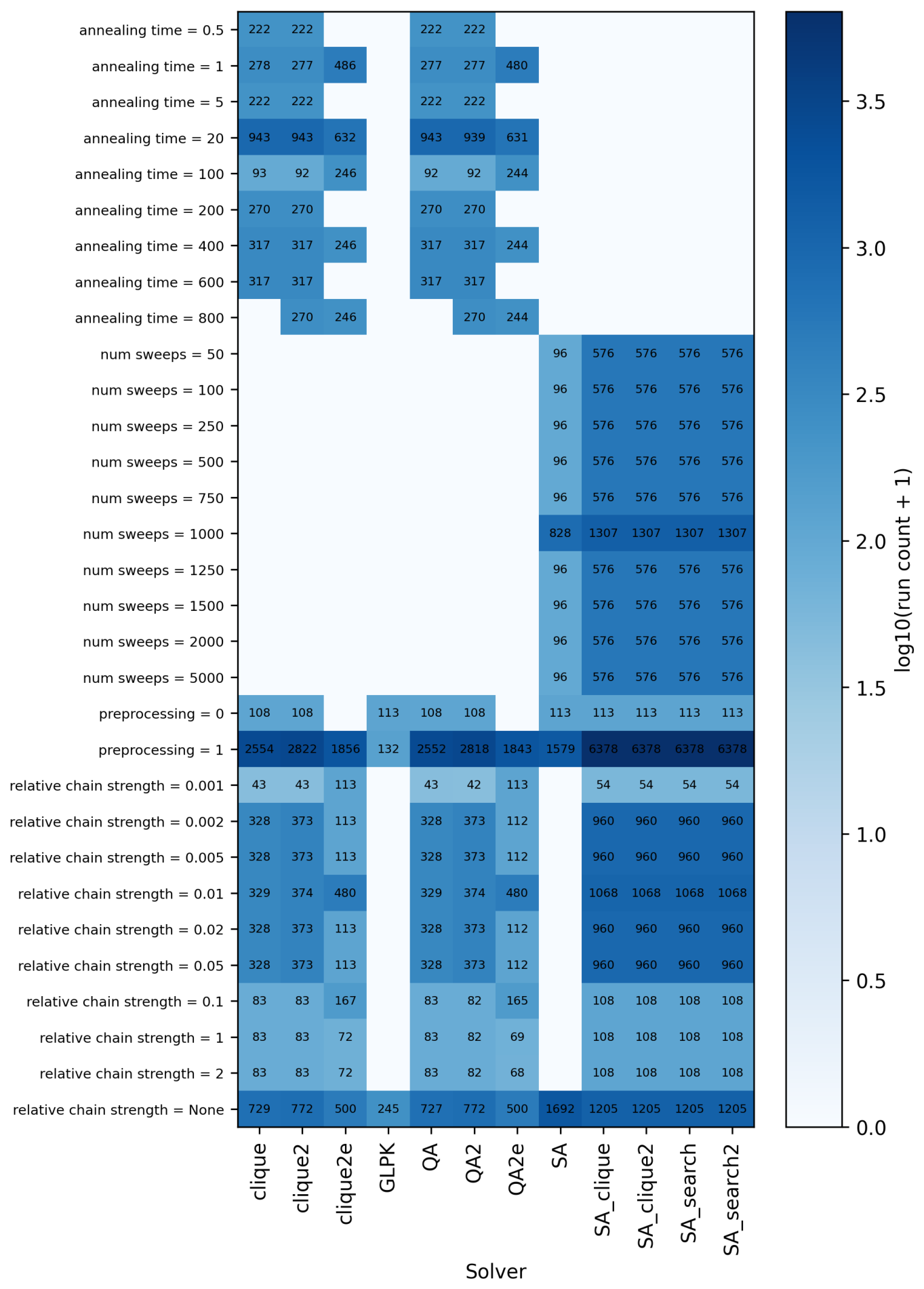
Appendix B. Penalty Statistics
Recall that in our Benders pipeline the QUBO penalty coefficients are updated each iteration according to the Big-M heuristics, ensuring that only feasible master solutions correspond to the lowest-energy QUBO solutions. In Figure A2 we showcase the evolution of these penalties during the Benders runs, only considering runs with at least 4 iterations. While for many cases the penalty remains unchanged, in the median it increases only once at the second iteration. This is because from the second iteration custom feasibility cuts or optimality cuts are added to the master problem. Not included in the previously highlighted results, we ran some runs with constant relative penalties, e.g., valued at 1. This, however, did neither improve nor decrease the performance on average. Hence, for consistency we restricted to the dynamic penalties in Section 3.
Figure A2.
Evolution of the relative big-M penalty over Benders iterations for the default-parameter runs. For the relative penalty, 1 corresponds to the default TSP penalty, which is the largest travel cost. (Left) balanced panel—only runs with ≥4 iterations are kept and truncated at 4, so every iteration contains the same runs (no survivor bias); thin gray lines are individual runs, blue is median with interquartile range. (Right) within-run change M(last) − M(first).
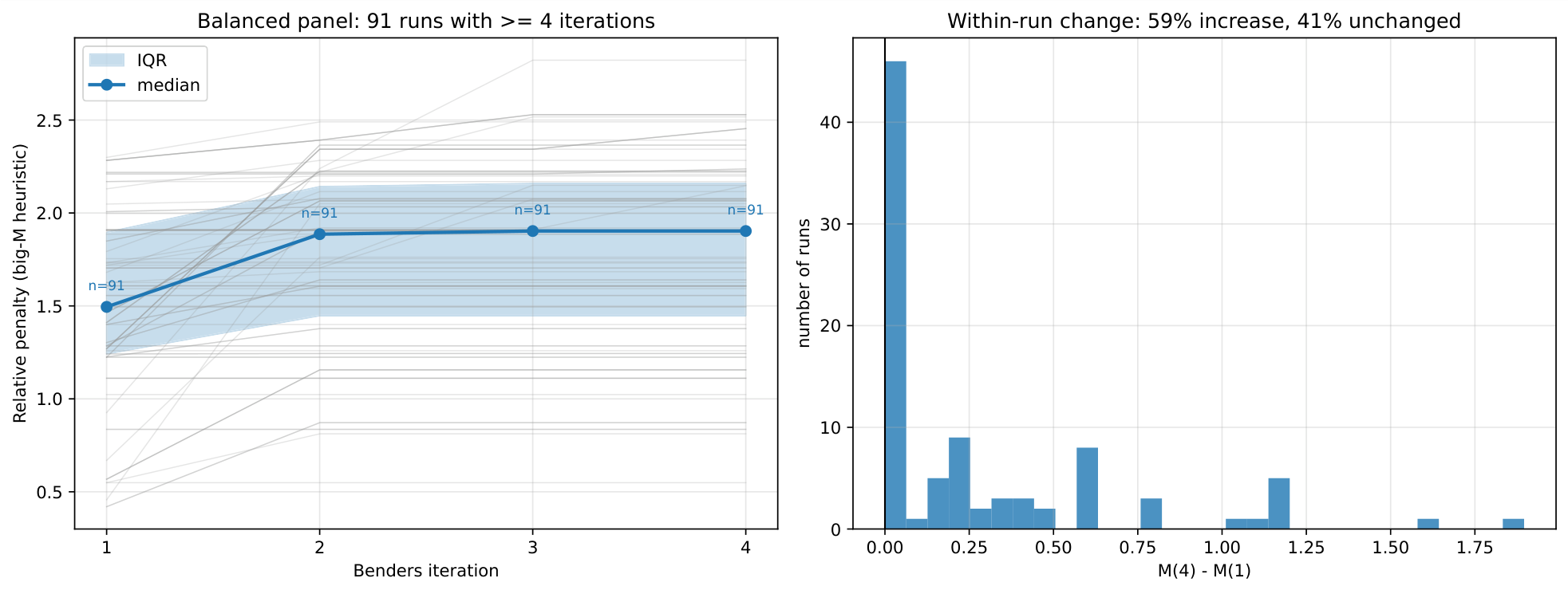
Appendix C. Instance Generation
The generated instances were partly based on operational data provided by the Harren Group. In particular, a distance matrix representing the approximate travel distances for 18 ports around the Gulf of Mexico and eastern South America was used. To protect commercially sensitive information, detailed information on the underlying data, in particular on individual ports, distances and storage costs, is not provided and only numerical ranges are stated. The distances in the underlying matrix range from 19 to 5544 nautical miles. Travel times were derived from the distance matrix using fixed sailing speeds of 10, 12, or 14 knots. The time-window and cost parameters were inspired by operational data of the Harren Group but generated synthetically.
To generate a random instance, first a specified number of ports (between 3 and 13) are randomly selected in addition to the depot port. Then, the size of the time window is chosen for each port within a range of the minimum time window size of 5 days and the maximum time window size of 10 days. The size is chosen from a beta distribution, with default parameters (, ) such that the sizes tend towards the average size.
Based on the generated time-window width, a delivery deadline is sampled uniformly for each customer port. The lower bound of this distribution is the travel time from the depot to the respective port plus the selected time-window width. Consequently, the start of the hard arrival-time window cannot occur before the vessel can reach the port directly from the depot, in accordance with the assumptions described in Section 2.1. The upper bound for the deadlines is chosen as the average travel time between distinct ports, multiplied by the number of ports n and a scaling factor, which is set to 2 by default.
To specify the time of earliest penalty-free arrival at a port, an offset between and 3 days before the respective deadline is sampled once again from a beta distribution with the same parameters as above. Storage-cost coefficients were chosen in a range of in the common cost unit per time unit. Sailing costs were set equal to sailing times, i.e., .
Finally, a specified number of customer ports may be selected to have no time-dependent delivery requirements. For these ports, the hard arrival-time window is extended to cover the interval from the earliest possible arrival time to the latest generated deadline plus the maximum travel time multiplied by the number of unconstrained ports. The share of ports without time windows was set to either or .
A feasibility check was performed using GLPK before an instance was retained, and only feasible instances were used.
Appendix D. Consistency Check and Error Estimate
As a consistency check, we compared the objective of every successful exact Benders run with default parameters to the optimum of the original MILP, which was obtained independently by solving the original formulation with the exact MILP solver. The 101 successful exact runs with default parameters cover –12. The 98 runs that terminated via the optimality-gap criterion all reproduce the MILP optimum, with a relative deviation below for every run. The remaining three runs stopped at the 100-iteration limit and are, therefore, not converged (one of them is 4.0% above the optimum). Since the exact baseline retains the continuous (Section 2.4.7), this check covers the decomposition and the cut generation, whereas the integer scaling of the cuts preserves the feasible set by construction (Section 2.4.4). The additional effect of the discretization on the stopping test is bounded by , as discussed in Section 2.4.7. Empirically, among the 769 default-parameter heuristic runs that terminated via the stopping test, 80.2% ended within 1% of the MILP optimum, 89.1% within 5%, and 92.5% within 10%.
Appendix E. Classical Hardware Information
The following hardware was used to run the pipeline and the associated classical computations, including subproblem solves, penalty coefficient generation and SA or GLPK master problem solves.
- CPU: AMD Ryzen Threadripper PRO 5965WX 24-Cores, 128 MB Cache, 48 Threads, 3.8 GHz to 4.5 GHz, 280 W
- Memory: 128 GB (4x32GB), DDR4, 3200 MHz
- GPU: NVIDIA RTX A6000
References
- Meurn, R.J. Marine Cargo Operations; Schiffer+ ORM: Atglen, PA, USA, 2011. [Google Scholar]
- Desrochers, M.; Lenstra, J.; Savelsbergh, M.; Soumis, F.; Golden, B.; Assad, A. Vehicle routing with time windows: Optimization and approximation. In Vehicle Routing: Methods and Studies; Golden, B.L., Assad, A.A., Eds.; North-Holland: Amsterdam, The Netherlands, 1988; pp. 65–84. [Google Scholar]
- Morita, S.; Nishimori, H. Mathematical foundation of quantum annealing. J. Math. Phys. 2008, 49, 125210. [Google Scholar] [CrossRef] [Scilit]
- Kim, S.; Ahn, S.W.; Suh, I.S.; Dowling, A.W.; Lee, E.; Luo, T. Quantum annealing for combinatorial optimization: A benchmarking study. npj Quantum Inf. 2025, 11, 77. [Google Scholar] [CrossRef] [Scilit]
- Quinton, F.A.; Myhr, P.A.S.; Barani, M.; Crespo del Granado, P.; Zhang, H. Quantum annealing applications, challenges and limitations for optimisation problems compared to classical solvers. Sci. Rep. 2025, 15, 12733. [Google Scholar] [CrossRef] [Scilit] [PubMed]
- McGeoch, C.C.; Farré, P. Milestones on the Quantum Utility Highway: Quantum Annealing Case Study. ACM Trans. Quantum Comput. 2023, 5, 1–30. [Google Scholar] [CrossRef] [Scilit]
- Huang, H.Y.; Choi, S.; McClean, J.R.; Preskill, J. The vast world of quantum advantage. arXiv 2025, arXiv:2508.05720. [Google Scholar] [CrossRef] [Scilit]
- Karp, R. Reducibility among Combinatorial Problems. In Complexity of Computer Computations; Springer: New York, NY, USA, 1972; Volume 10, pp. 85–103. [Google Scholar]
- Held, M.; Karp, R.M. A dynamic programming approach to sequencing problems. J. Soc. Ind. Appl. Math. 1962, 10, 196–210. [Google Scholar] [CrossRef] [Scilit]
- Applegate, D.; Bixby, R.; Chvátal, V.; Cook, W. The Traveling Salesman Problem: A Computational Study; Princeton University Press: Princeton, NJ, USA, 2006; pp. 154–196. [Google Scholar]
- Christofides, N. Worst-case Analysis of a New Heuristic for the Travelling Salesman Problem; Technical Report 388; Graduate School of Industrial Administration, Carnegie Mellon University: Pittsburgh, PA, USA, 1976. [Google Scholar]
- Arora, S. Polynomial Time Approximation Schemes for Euclidean Traveling Salesman and Other Geometric Problems. J. ACM 1998, 45, 753–782. [Google Scholar] [CrossRef] [Scilit]
- Lin, S.; Kernighan, B. An Effective Heuristic Algorithm for the Traveling-Salesman Problem. Oper. Res. 1973, 21, 498–516. [Google Scholar] [CrossRef] [Scilit]
- Helsgaun, K. An Effective Implementation of the Lin–Kernighan Traveling Salesman Heuristic. Eur. J. Oper. Res. 2000, 126, 106–130. [Google Scholar] [CrossRef] [Scilit]
- Reinelt, G. TSPLIB—A Traveling Salesman Problem Library. ORSA J. Comput. 1991, 3, 376–384. [Google Scholar] [CrossRef] [Scilit]
- Lucas, A. Ising formulations of many NP problems. Front. Phys. 2014, 2, 5. [Google Scholar] [CrossRef] [Scilit]
- Farhi, E.; Goldstone, J.; Gutmann, S. A Quantum Approximate Optimization Algorithm. arXiv 2014, arXiv:1411.4028. [Google Scholar] [CrossRef] [Scilit]
- Kirkpatrick, S.; Gelatt, C.D.; Vecchi, M.P. Optimization by Simulated Annealing. Science 1983, 220, 671–680. [Google Scholar] [CrossRef] [Scilit] [PubMed]
- Ohlmann, J.W.; Thomas, B.W. A Compressed Annealing Approach to the Traveling Salesman Problem with Time Windows. INFORMS J. Comput. 2007, 19, 410–420. [Google Scholar] [CrossRef] [Scilit]
- Solomon, M.M. Algorithms for the Vehicle Routing and Scheduling Problems with Time Window Constraints. Oper. Res. 1987, 35, 254–265. [Google Scholar] [CrossRef] [Scilit]
- Papalitsas, C.; Andronikos, T.; Giannakis, K.; Theocharopoulou, G.; Fanarioti, S. A QUBO Model for the Traveling Salesman Problem with Time Windows. Algorithms 2019, 12, 224. [Google Scholar] [CrossRef] [Scilit]
- Salehi, Ö.; Glos, A.; Miszczak, J.A. Unconstrained binary models of the travelling salesman problem variants for quantum optimization. Quantum Inf. Process. 2022, 21, 67. [Google Scholar] [CrossRef] [Scilit]
- Anthony, M.; Boros, E.; Crama, Y.; Gruber, A. Quadratic reformulations of nonlinear binary optimization problems. Math. Program. 2017, 162, 115–144. [Google Scholar] [CrossRef] [Scilit]
- Osaba, E.; Villar-Rodriguez, E.; Oregi, I. A Systematic Literature Review of Quantum Computing for Routing Problems. IEEE Access 2022, 10, 55805–55817. [Google Scholar] [CrossRef] [Scilit]
- Martoňák, R.; Santoro, G.E.; Tosatti, E. Quantum annealing of the traveling-salesman problem. Phys. Rev. E 2004, 70, 057701. [Google Scholar] [CrossRef] [Scilit] [PubMed]
- Crispin, A.; Syrichas, A. Quantum Annealing Algorithm for Vehicle Scheduling. In Proceedings of the 2013 IEEE International Conference on Systems, Man, and Cybernetics; IEEE: Piscataway, NJ, USA, 2013; pp. 3523–3528. [Google Scholar] [CrossRef] [Scilit]
- Le, T.V.; Nguyen, M.V.; Khandavilli, S.; Dinh, T.N.; Nguyen, T.N. Quantum Annealing Approach for Selective Traveling Salesman Problem. In Proceedings of the ICC 2023-IEEE International Conference on Communications; IEEE: Piscataway, NJ, USA, 2023; pp. 2686–2691. [Google Scholar] [CrossRef] [Scilit]
- Holliday, J.; Blount, D.; Osaba, E.; Luu, K. Advanced Quantum Annealing Approach to Vehicle Routing Problems with Time Windows. arXiv 2025, arXiv:2503.24285. [Google Scholar] [CrossRef] [Scilit]
- Benders, J.F. Partitioning procedures for solving mixed-variables programming problems. Numer. Math. 1962, 4, 238–252. [Google Scholar] [CrossRef] [Scilit]
- Hooker, J.N.; Ottosson, G. Logic-based Benders decomposition. Math. Program. 2003, 96, 33–60. [Google Scholar] [CrossRef] [Scilit]
- Shahidehpour, M.; Fu, Y. Benders decomposition: Applying Benders decomposition to power systems. IEEE Power Energy Mag. 2005, 3, 20–21. [Google Scholar] [CrossRef] [Scilit]
- Belieres, S.; Hewitt, M.; Jozefowiez, N.; Semet, F.; Van Woensel, T. A Benders decomposition-based approach for logistics service network design. Eur. J. Oper. Res. 2020, 286, 523–537. [Google Scholar] [CrossRef] [Scilit]
- Cappanera, P.; Gavanelli, M.; Nonato, M.; Roma, M. Logic-Based Benders Decomposition in Answer Set Programming for Chronic Outpatients Scheduling. Theory Pract. Log. Program. 2023, 23, 848–864. [Google Scholar] [CrossRef] [Scilit]
- Chang, C.Y.; Jones, E.; Yao, Y.; Graf, P.; Jain, R. On hybrid quantum and classical computing algorithms for mixed-integer programming. arXiv 2020, arXiv:2010.07852. [Google Scholar]
- Zhao, Z.; Fan, L.; Han, Z. Hybrid Quantum Benders’ Decomposition For Mixed-integer Linear Programming. In Proceedings of the 2022 IEEE Wireless Communications and Networking Conference (WCNC); IEEE: Piscataway, NJ, USA, 2022; pp. 2536–2540. [Google Scholar] [CrossRef] [Scilit]
- Leenders, L.; Sollich, M.; Reinert, C.; Bardow, A. Integrating quantum and classical computing for multi-energy system optimization using Benders decomposition. Comput. Chem. Eng. 2024, 188, 108763. [Google Scholar] [CrossRef] [Scilit]
- Naghmouchi, M.Y.; Coelho, W.d.S. Mixed-integer linear programming solver using Benders decomposition assisted by a neutral-atom quantum processor. Phys. Rev. A 2024, 110, 012434. [Google Scholar] [CrossRef] [Scilit]
- Zhao, Z.; Fan, L.; Guo, Y.; Wang, Y.; Han, Z.; Hanzo, L. QAOA-Assisted Benders’ Decomposition for Mixed-integer Linear Programming. In Proceedings of the ICC 2024-IEEE International Conference on Communications; IEEE: Piscataway, NJ, USA, 2024; pp. 1127–1132. [Google Scholar] [CrossRef] [Scilit]
- Gao, F.; Huang, D.; Zhao, Z.; Dai, W.; Yang, M.; Gao, Q.; Pan, Y. Fully and partially distributed Quantum Generalized Benders Decomposition for Unit Commitment Problems. arXiv 2022, arXiv:2210.06678. [Google Scholar] [CrossRef] [Scilit]
- Dibbern, J.; Szal, O.; Rizvanolli, A. From MINLP to QUBO: A Quantum-Inspired Approach for Bulk Carrier Routing with Time Windows. In Proceedings of the 23rd International Conference on Computer and IT Applications in the Maritime Industries COMPIT’25; Hamburg University of Technology: Hamburg, Germany, 2025. [Google Scholar]
- Hungerländer, P.; Truden, C. Efficient and Easy-to-Implement Mixed-Integer Linear Programs for the Traveling Salesperson Problem with Time Windows. Transp. Res. Procedia 2018, 30, 157–166. [Google Scholar] [CrossRef] [Scilit]
- Tamura, K.; Shirai, T.; Katsura, H.; Tanaka, S.; Togawa, N. Performance Comparison of Typical Binary-Integer Encodings in an Ising Machine. IEEE Access 2021, 9, 81032–81039. [Google Scholar] [CrossRef] [Scilit]
- Achterberg, T.; Bixby, R.E.; Gu, Z.; Rothberg, E.; Weninger, D. Presolve Reductions in Mixed Integer Programming. INFORMS J. Comput. 2020, 32, 473–506. [Google Scholar] [CrossRef] [Scilit]
- Alessandroni, E.; Ramos-Calderer, S.; Roth, I.; Traversi, E.; Aolita, L. Alleviating the quantum Big-M problem. npj Quantum Inf. 2025, 11, 125. [Google Scholar] [CrossRef] [Scilit]
- Makhorin, A. GLPK (GNU Linear Programming Kit), Version 5.0. Available online: http://www.gnu.org/software/glpk/glpk.html (accessed on 1 September 2026).
- O’Donoghue, B.; Chu, E.; Parikh, N. SCS: Splitting Conic Solver, Version 3.2.9. 2025. Available online: https://github.com/cvxgrp/scs (accessed on 6 February 2026).
- Boros, E.; Hammer, P.L.; Tavares, G. Preprocessing of Unconstrained Quadratic Binary Optimization; Technical Report RRR 10-2006, Rutcor Research Report; Rutgers Center for Operations Research, Rutgers University: Piscataway, NJ, USA, 2006. [Google Scholar]
- D-Wave. Roof Duality. Available online: https://docs.dwavequantum.com/en/latest/ocean/api_ref_preprocessing/api_ref.html#dwave.preprocessing.lower_bounds.roof_duality (accessed on 1 September 2026).
- Boothby, T.; King, A.D.; Roy, A. Fast clique minor generation in Chimera qubit connectivity graphs. Quantum Inf. Process. 2016, 15, 495–508. [Google Scholar] [CrossRef] [Scilit]
- D-Wave. Minorminer. Available online: https://docs.dwavequantum.com/en/latest/ocean/api_ref_minorminer/source/index.html (accessed on 1 July 2026).
- Cai, J.; Macready, W.G.; Roy, A. A practical heuristic for finding graph minors. arXiv 2014, arXiv:1406.2741. [Google Scholar] [CrossRef] [Scilit]
- Albash, T.; Lidar, D.A. Demonstration of a Scaling Advantage for a Quantum Annealer over Simulated Annealing. Phys. Rev. X 2018, 8, 031016. [Google Scholar] [CrossRef] [Scilit]
- López-Baños, S.; Lobe, E.; Lünsdorf, O.; Raventós, O. Performance enhancing of hybrid quantum-classical Benders approach for MILP optimization. arXiv 2026, arXiv:2601.14024. [Google Scholar] [CrossRef] [Scilit]
- Hamburg Soll an Die Spitze im Quantencomputing. 2022. Available online: https://www.hamburg.de/bwi/medien/16613674/2022-10-25-bwi-quantencomputing/ (accessed on 30 September 2026).
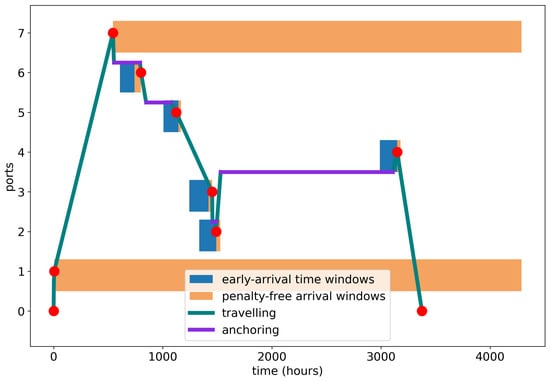
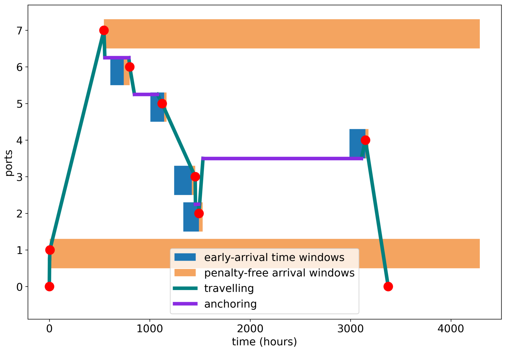
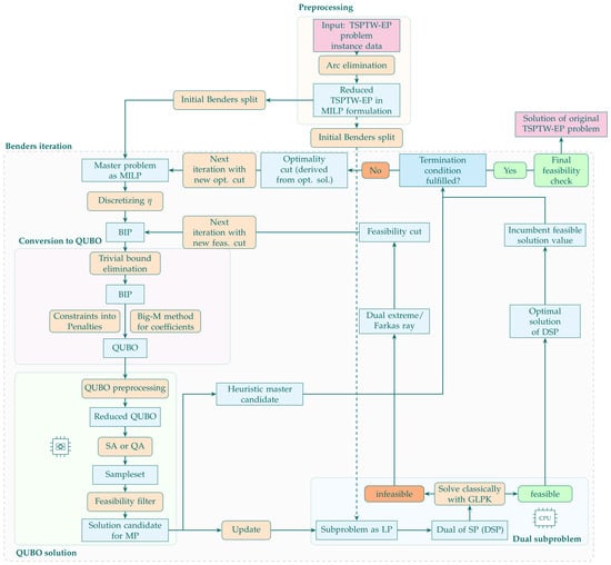
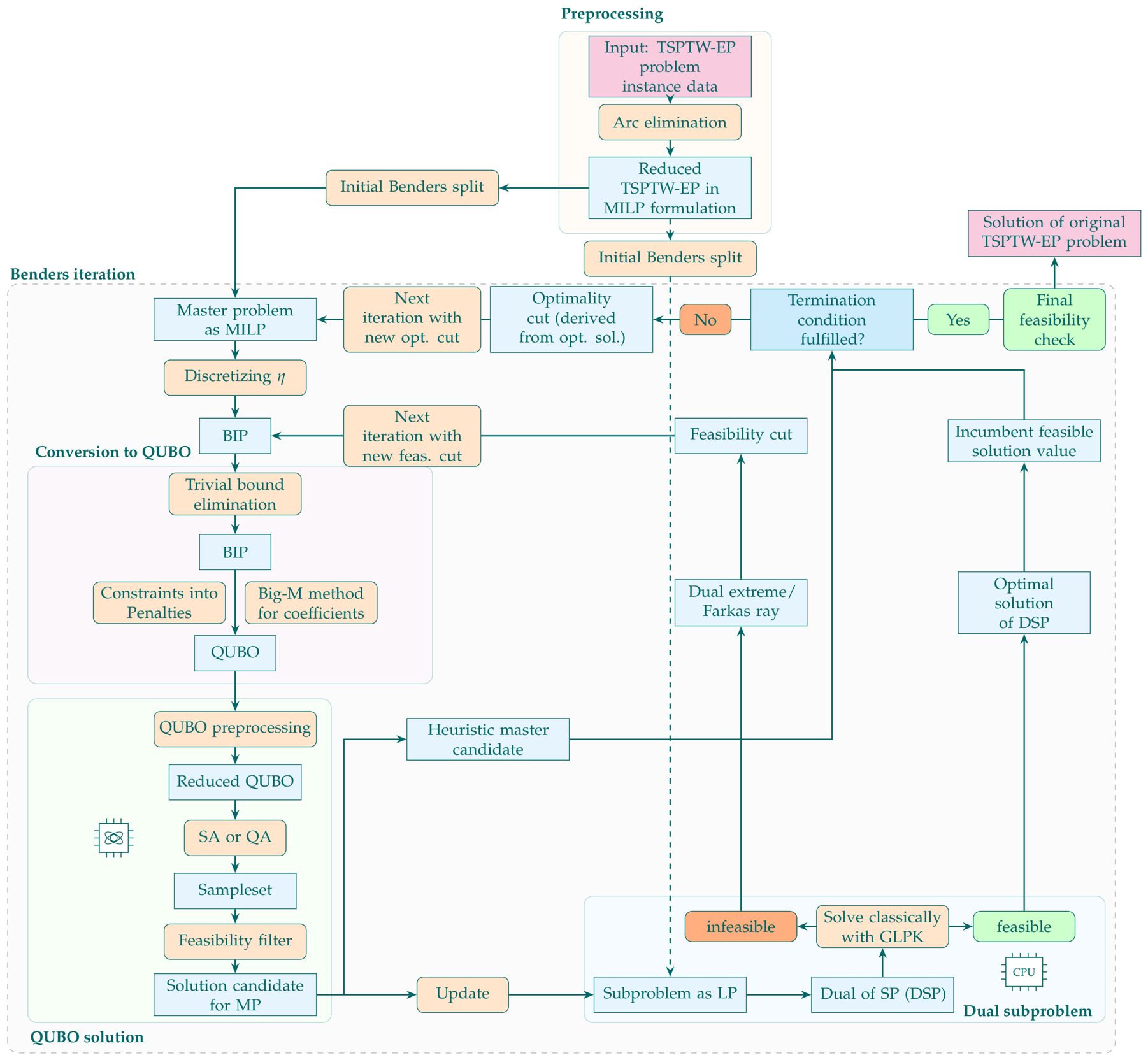
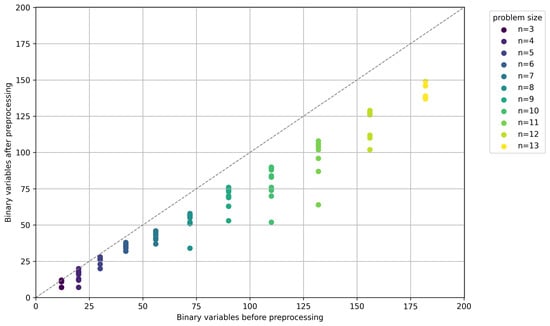
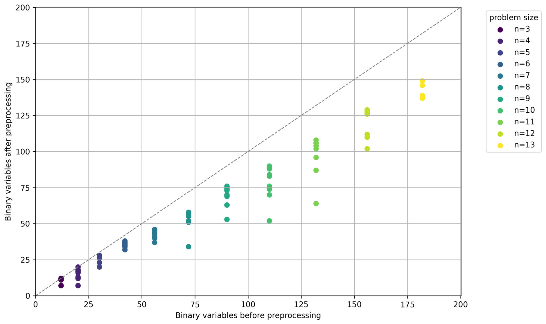
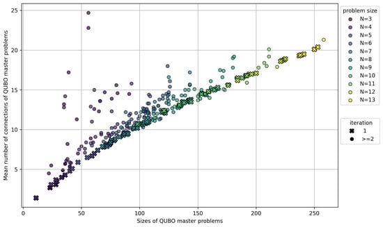
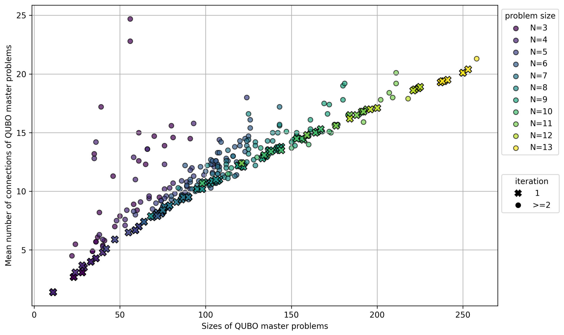
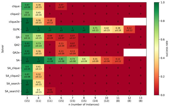
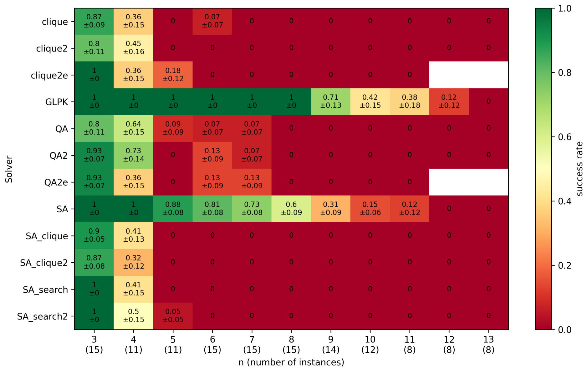
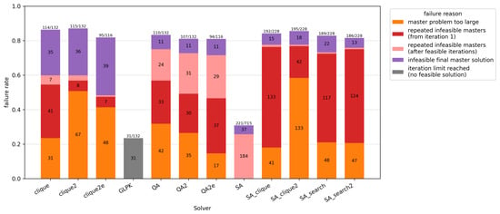
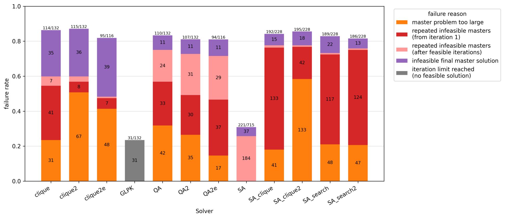
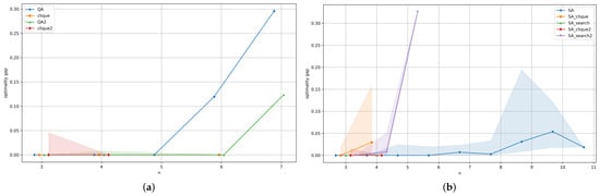
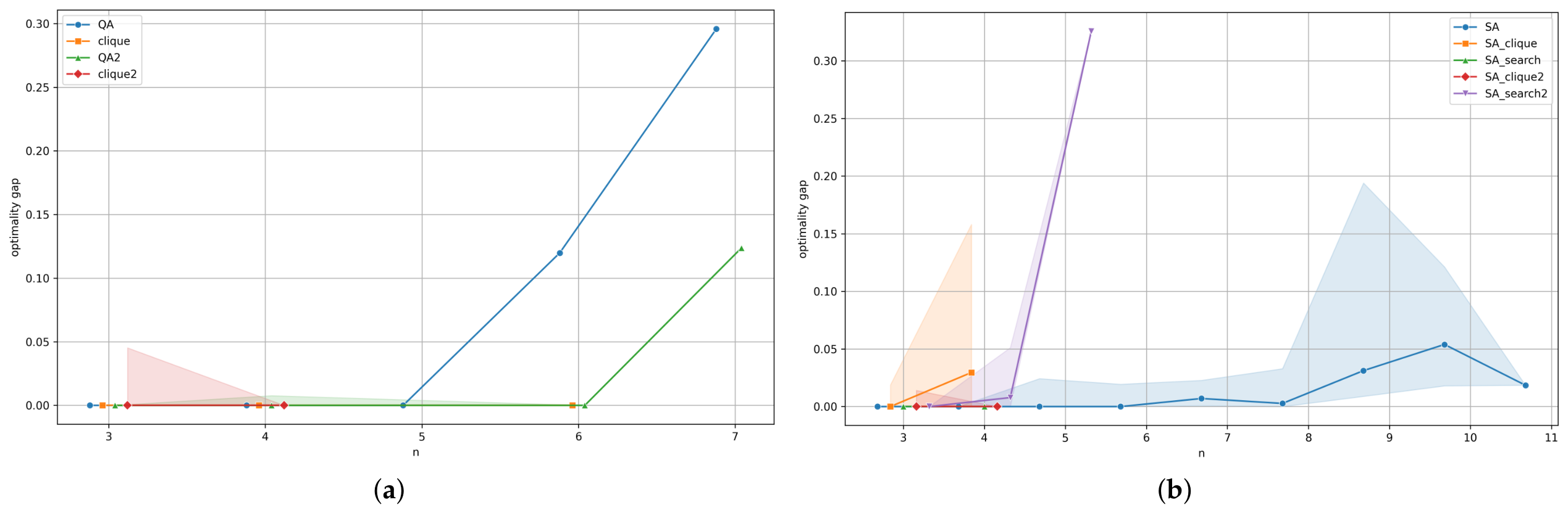
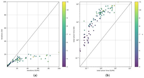
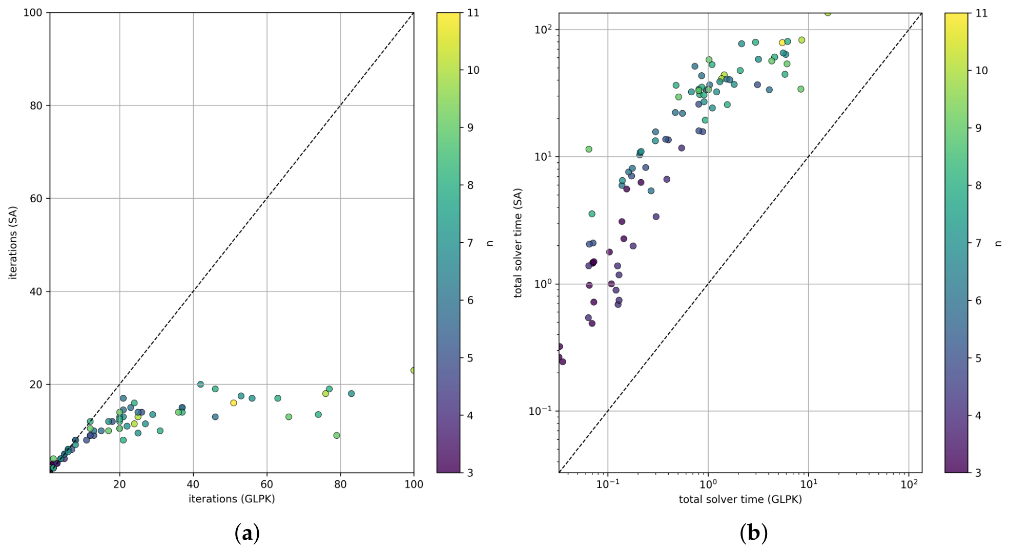
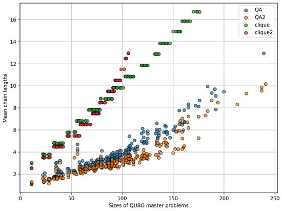
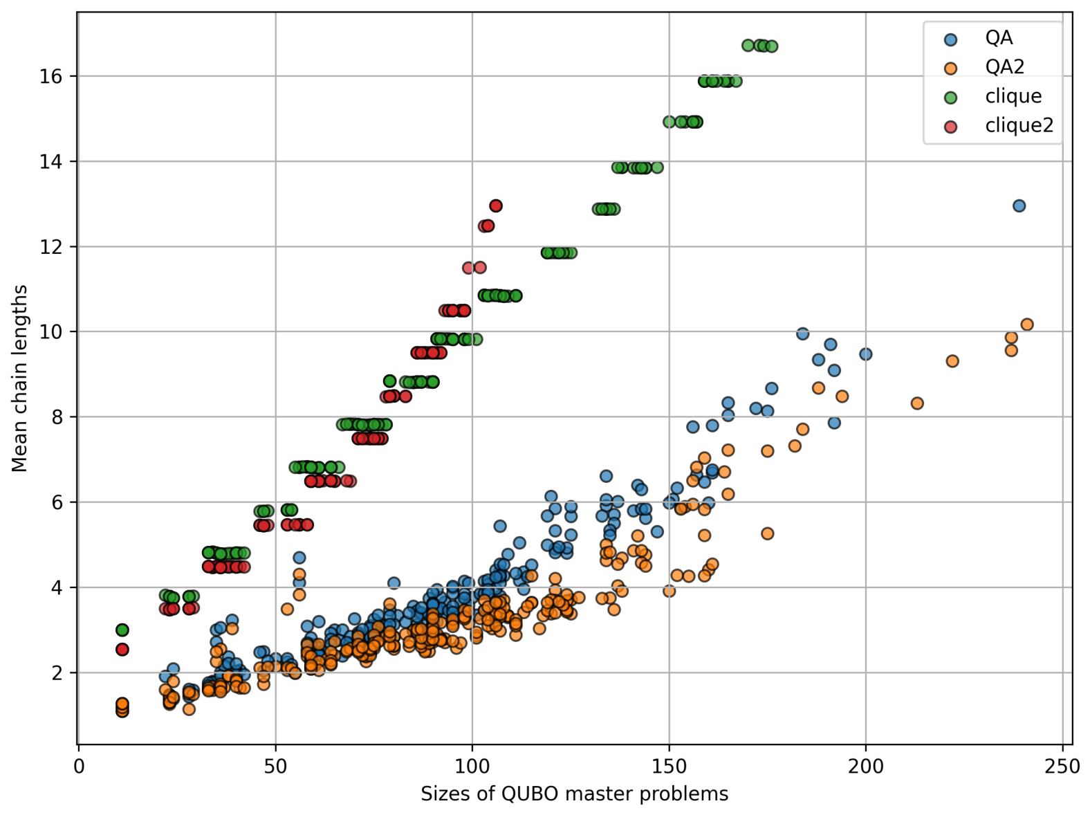
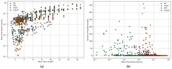
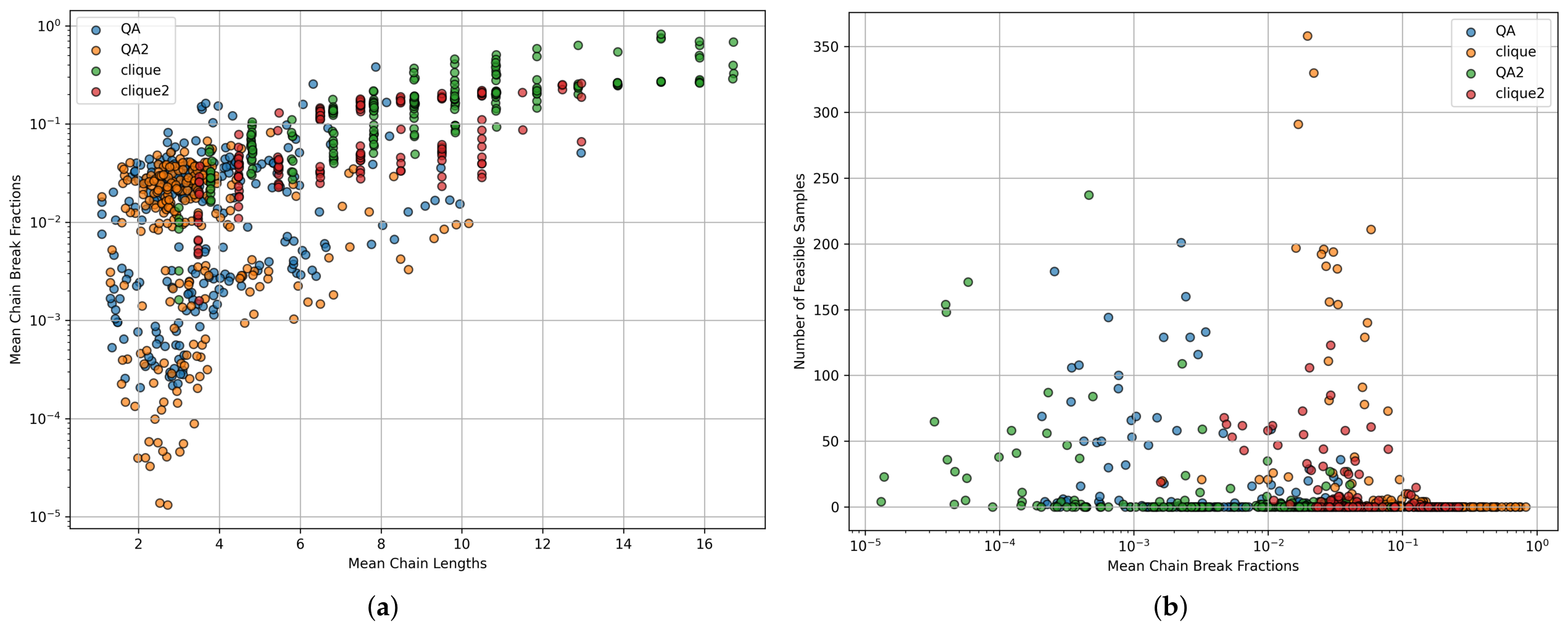
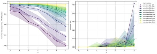
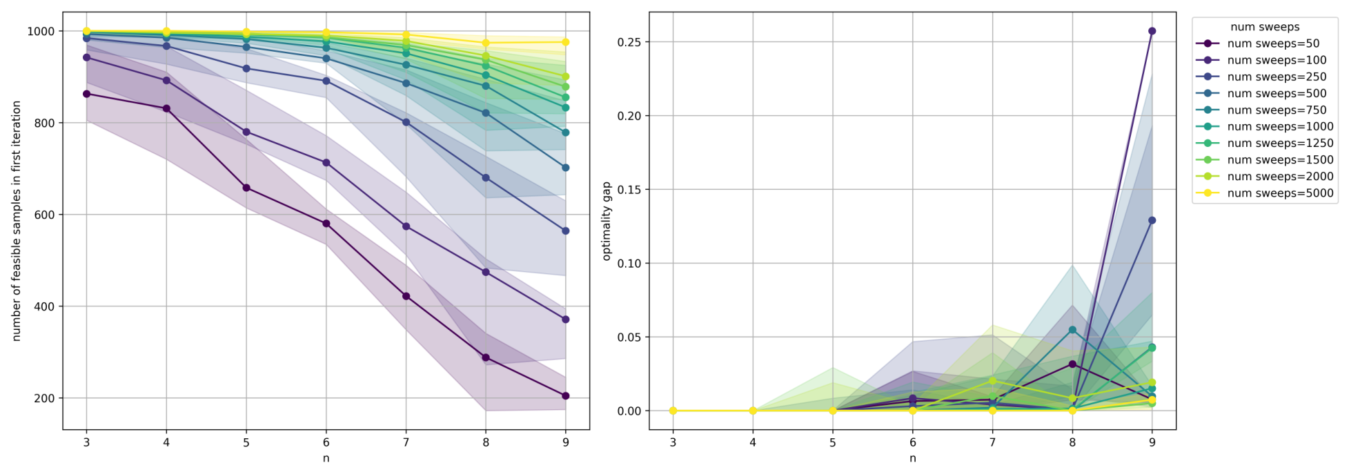
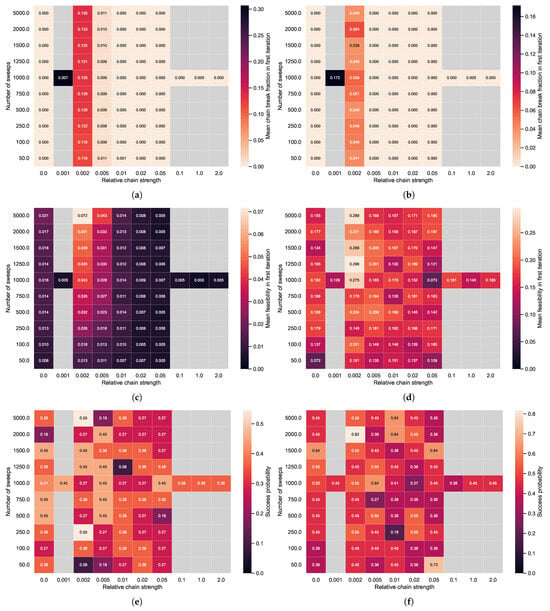
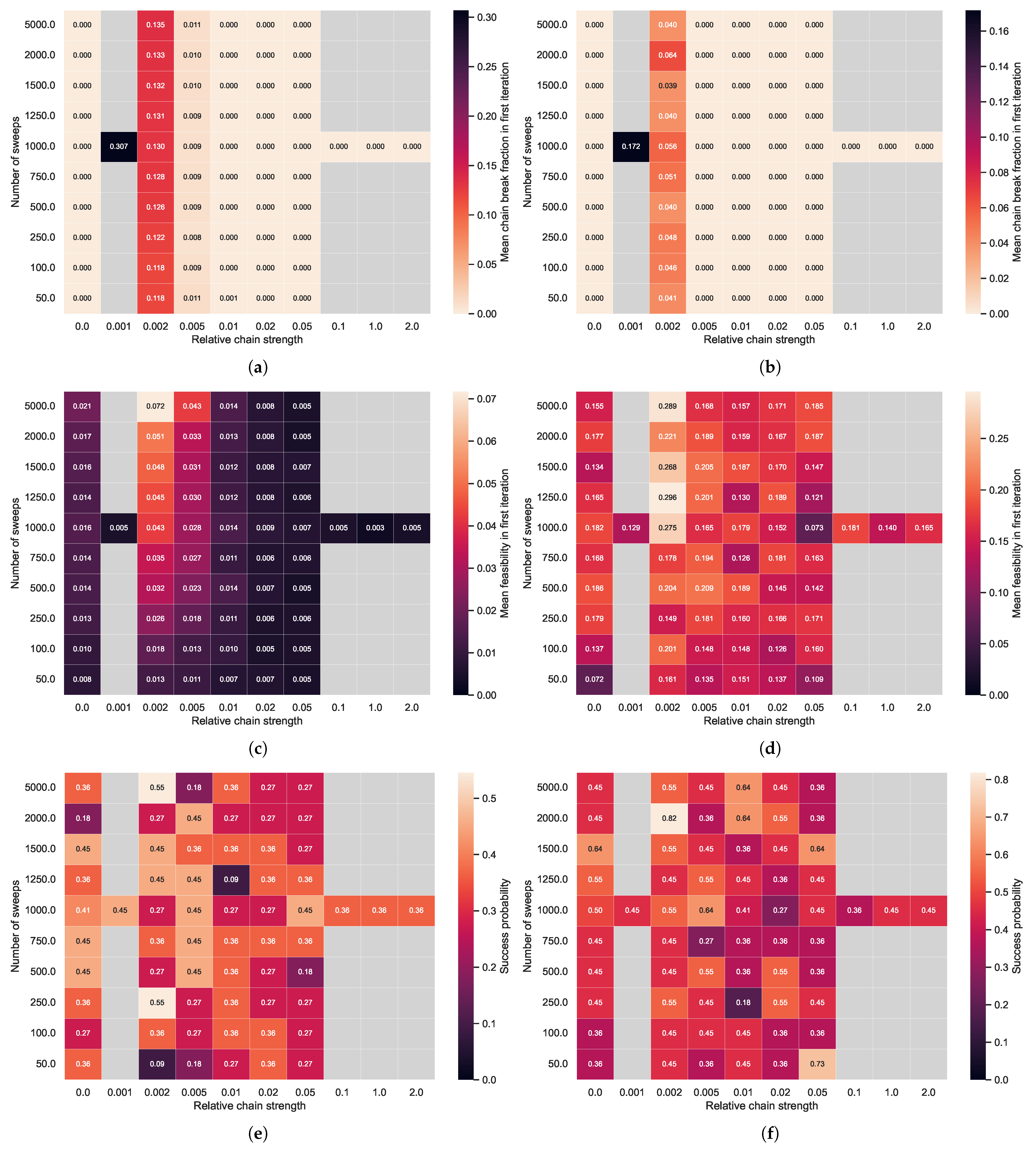
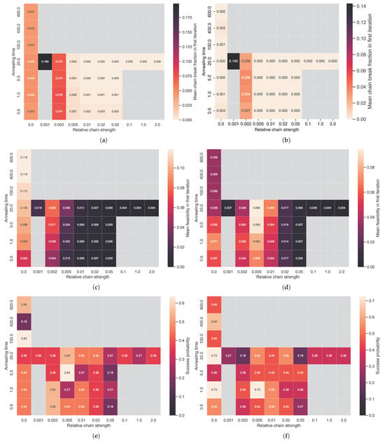
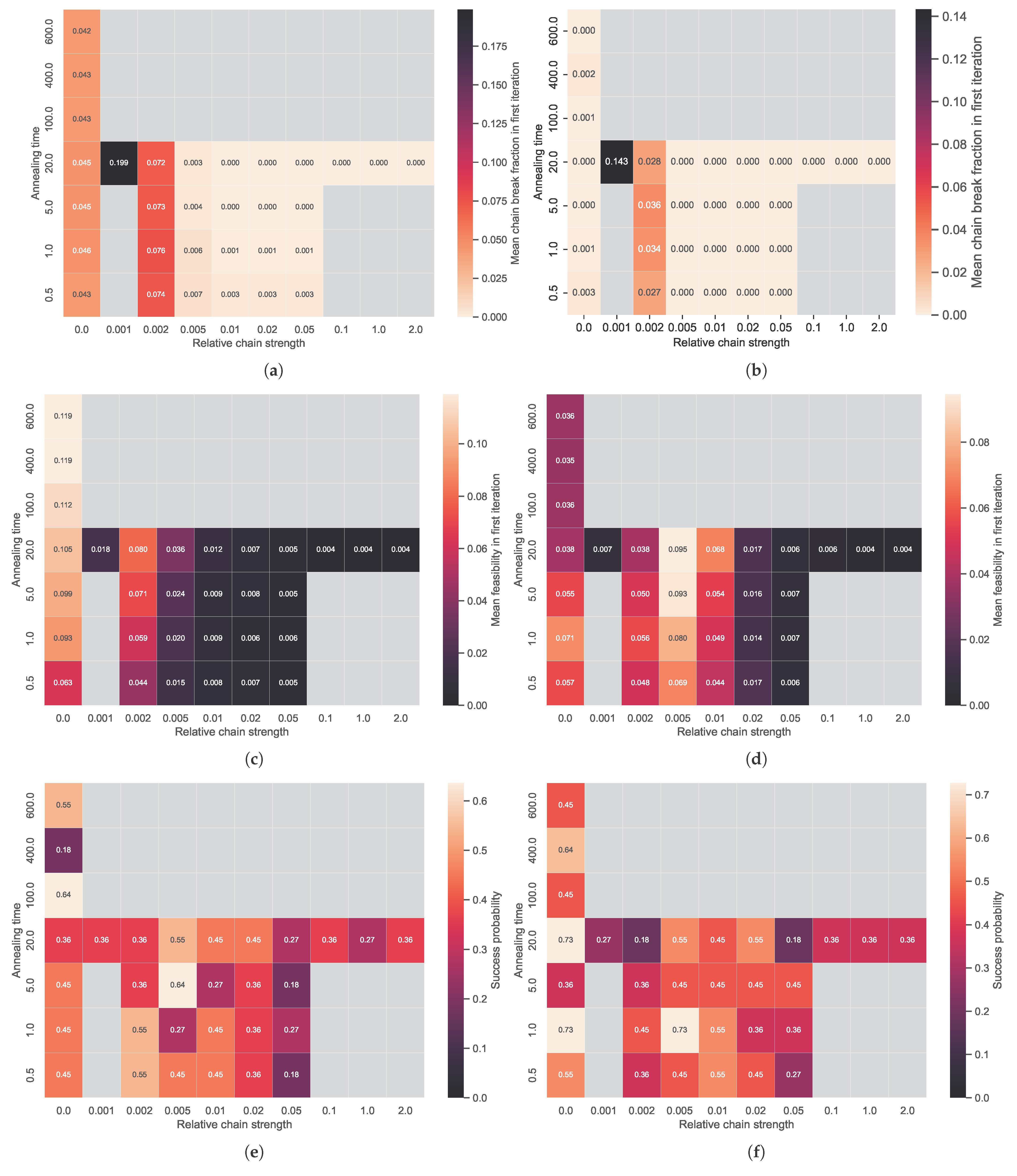

Disclaimer/Publisher’s Note: The statements, opinions and data contained in all publications are solely those of the individual author(s) and contributor(s) and not of MDPI and/or the editor(s). MDPI and/or the editor(s) disclaim responsibility for any injury to people or property resulting from any ideas, methods, instructions or products referred to in the content. |
© 2026 by the authors. Licensee MDPI, Basel, Switzerland. This article is an open access article distributed under the terms and conditions of the Creative Commons Attribution (CC BY) license.