Problems of Automated Control of Viral Disease Progression Accounting for Spatial Perturbations and Body Temperature Response Under Immunotherapy

Abstract

We develop a spatiotemporal mathematical model describing viral infection dynamics under the combined effects of diffusion, convection, temperature-dependent immune response, and therapeutic intervention. The model is formulated as a system of singularly perturbed delay partial differential equations that captures the interactions among viral particles, immune agents, target-organ damage, and body-temperature regulation. To efficiently compute approximate solutions, we propose a hybrid asymptotic–numerical framework that combines the method of steps with singular perturbation techniques. The delayed system is transformed into a sequence of auxiliary non-delay problems, allowing the systematic construction of computationally efficient approximations while preserving the essential multiscale characteristics of the original model. An adaptive control strategy is introduced to regulate immunological and antipyretic therapies based on predicted system evolution. Numerical experiments are performed to investigate the effects of treatment timing, dosage, and temperature regulation on infection progression. The simulations demonstrate that early therapeutic intervention improves viral suppression, whereas excessive temperature reduction may diminish the protective effects of the febrile response and lead to less favorable outcomes. The proposed framework provides an efficient computational tool for the analysis and control of spatially distributed infection dynamics and represents a step toward the development of personalized treatment strategies based on predictive mathematical modeling.

1. Introduction

Personalized medicine and targeted therapeutic interventions have become increasingly important in the treatment of infectious diseases. Advances in biotechnology, medical monitoring, and computational modeling have created new opportunities for predicting disease progression and adapting treatment strategies to individual patients. Mathematical models play an important role in this process by providing a systematic framework for studying interactions among pathogens, immune responses, physiological regulation mechanisms, and therapeutic interventions. Such interactions are often difficult to assess directly through clinical observation or laboratory experimentation.

Despite substantial progress in mathematical immunology, many existing models remain limited in their ability to simultaneously incorporate spatial heterogeneity, delayed immune responses, and physiological feedback mechanisms. Spatial effects arise naturally from the non-uniform distribution of viral particles, immune cells, and therapeutic agents within biological tissues, while delays are inherent in immune activation and antibody production. In addition, physiological processes such as body-temperature regulation can substantially influence pathogen replication and treatment outcomes. The integration of these mechanisms into a unified computational framework remains an important challenge.

Accurate prediction of infection dynamics requires accounting for convection–diffusion transport and localized interactions between biological agents. Although several spatial models of immune response have been proposed [1,2,3,4], most studies focus primarily on diffusion-driven transport or compartmental representations of spatial structure [5]. Alternative approaches developed in [6] incorporated small diffusion effects, while subsequent studies [7] examined the influence of diffusion perturbations under pharmacological and immunological therapies. These models were later extended to include localized therapeutic interventions and concentrated drug-administration regimes [8].

Another important component of infection dynamics is the body’s febrile response. Elevated temperature is a natural protective mechanism that suppresses pathogen replication and contributes to immune defense. Mathematical models incorporating temperature-dependent effects have demonstrated that thermal regulation may substantially influence disease progression and treatment efficacy. In [9], diffusion perturbations, immunotherapy, and temperature effects were incorporated into a generalized infection model, while [10] further extended the framework to include adsorption-based therapeutic interventions.

While existing studies have provided valuable insights into individual aspects of infection dynamics, most models address spatial transport, physiological feedback, or therapeutic control separately. Reaction–diffusion models often neglect delayed immune responses and adaptive treatment mechanisms, whereas control-oriented models are frequently restricted to low-dimensional systems and do not account for spatial heterogeneity. Consequently, there remains a need for computationally efficient modeling frameworks that simultaneously integrate diffusion, convection, delay effects, temperature regulation, and therapeutic control.

In this study, we develop a spatiotemporal framework for analyzing and controlling viral infection dynamics that combines these features within a single mathematical model. The proposed approach is based on a system of singularly perturbed delay partial differential equations describing the interactions among viral particles, immune agents, target-organ damage, and body temperature. To efficiently analyze the resulting system, we develop a hybrid asymptotic–numerical methodology that combines the method of steps with singular perturbation techniques.

The main contributions of this work are summarized as follows:

• Model development. We formulate a spatially distributed model of viral infection dynamics that incorporates diffusion perturbations, convection transport, delay effects, temperature-dependent immune regulation, and therapeutic interventions.
• Computational methodology. We develop a hybrid asymptotic–numerical framework that transforms the original delayed system into a sequence of auxiliary non-delay problems while preserving the dominant multiscale dynamics.
• Adaptive control. We introduce a computationally tractable adaptive control strategy for regulating immunological and antipyretic therapies based on predicted disease progression and physiological constraints.
• Numerical investigation. We evaluate the influence of treatment timing, treatment intensity, temperature regulation, and diffusion effects on infection progression through a series of numerical experiments.

Together, these contributions provide a unified framework for the modeling, simulation, and control of spatially distributed infection dynamics and offer a foundation for future studies on personalized treatment optimization.

Compared with previous immune-response models, the proposed framework simultaneously incorporates spatial transport, delay effects, temperature-dependent physiological regulation, and adaptive therapeutic control within a single modeling environment. This integration permits the investigation of interactions among these mechanisms while maintaining computational tractability through the proposed asymptotic–numerical methodology.

The remainder of the paper is organized as follows. Section 2 introduces the mathematical model. Section 3 presents the asymptotic–numerical solution framework. Section 4 describes the adaptive control strategy. Section 5 presents numerical experiments, and Section 6 concludes the paper with a discussion of the main findings and future research directions.

2. Mathematical Model

We begin with the classical antiviral immune-response model proposed in [11], which is formulated as a system of four delay differential equations describing the interactions between viral particles and the host immune system.

$$\begin{array}{c}{\displaystyle \frac{\partial V}{\partial t}}=(\mathrm{\beta }-\mathrm{\gamma }F)V,\\ {\displaystyle \frac{\partial C}{\partial t}}=\mathrm{\xi }(m)\mathrm{\alpha }F(t-\mathrm{\tau })V(t-\mathrm{\tau })-{\mathrm{\mu }}_C(C-C^{*}),\\ {\displaystyle \frac{\partial F}{\partial t}}=\mathrm{\rho }C-({\mathrm{\mu }}_f+\mathrm{\eta }\mathrm{\gamma }V)F,\\ {\displaystyle \frac{\partial m}{\partial t}}=\mathrm{\sigma }V-{\mathrm{\mu }}_{m}m.\end{array}$$

The state variables of the model include the concentration of antigens $V(t)$ (pathogenic viruses), specific immune agents $F(t)$ (antibodies, cell receptors, etc.), immunocompetent cells $C(t)$ (antibody producers), and a characteristic measure of target organ damage $m(t)$. The model is based on F.M. Burnet’s clonal selection theory [12], in which the humoral immune response is initiated by the activation of specific lymphocytes upon binding to antigens. Following activation and a characteristic time delay, these lymphocytes proliferate to form a clonal population that produces antibodies to neutralize the antigen. Qualitative analysis of this baseline model has identified key disease regimes—subclinical, acute, and chronic—which are in qualitative agreement with clinical observations.

Owing to its biological interpretability, the model has been extended in numerous studies to investigate different disease processes, immune-response mechanisms, and therapeutic interventions [13,14,15,16,17,18]. In particular, the framework has been adapted to describe tumor–immune interactions [14] and more recently to study the effects of immunotherapy in COVID-19 infection dynamics [18].

While the baseline model captures the essential temporal interactions between viral dynamics and immune responses, it does not account for spatial heterogeneity arising from transport processes and localized biological interactions. In biological tissues, viral particles, immune agents, and therapeutic compounds are generally distributed non-uniformly and evolve under the combined effects of diffusion, convection, and localized interventions. To account for these mechanisms, we extend the original model to a spatiotemporal framework.

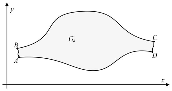
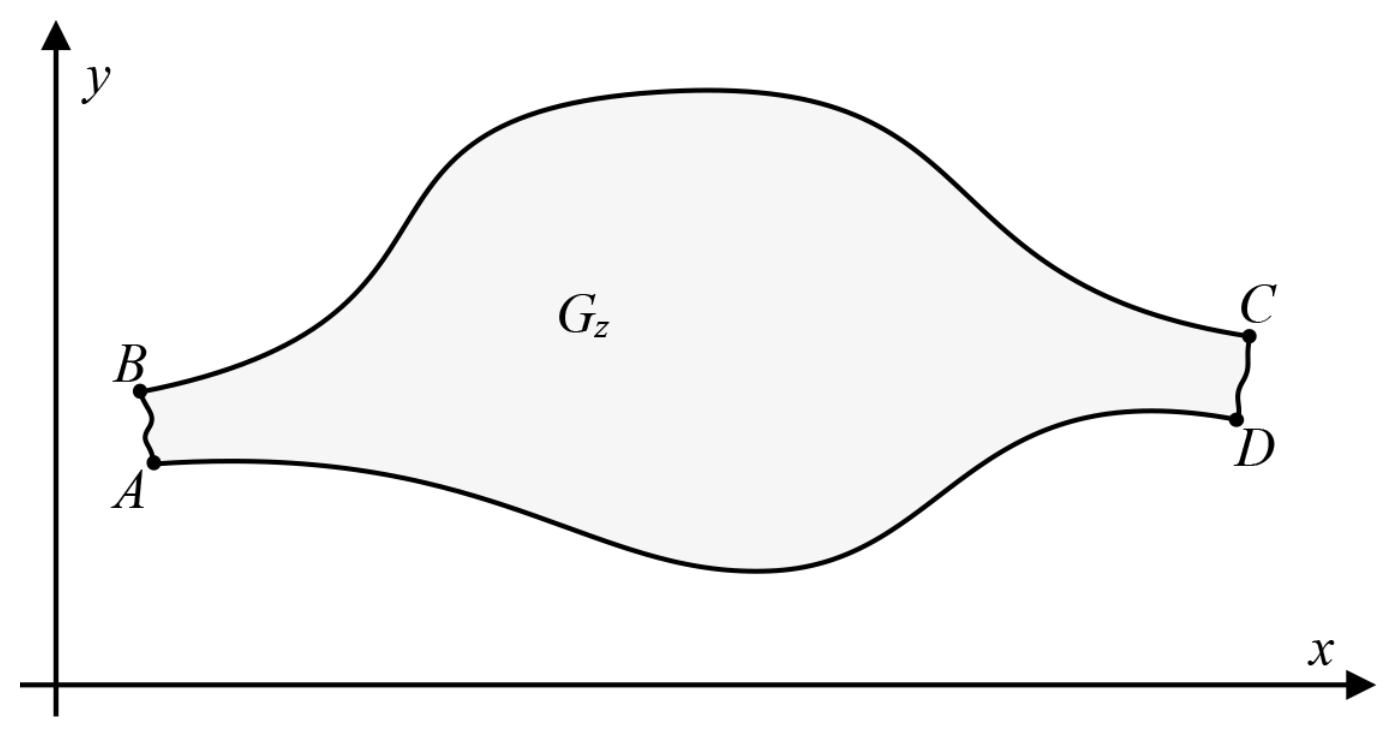
The model is formulated on a bounded two-dimensional domain $G_z$, represented by a curvilinear quadrilateral bounded by smooth curves (Figure 1). The resulting spatiotemporal dynamics are described by the singularly perturbed system (1) subject to conditions (2).

$$\begin{array}{c}{\displaystyle \frac{\partial V}{\partial t}}=w^V+(\mathrm{\beta }(\mathrm{\theta })-\mathrm{\gamma }F)V-{\mathrm{\upsilon }}_x^V{\displaystyle \frac{\partial V}{\partial x}}-{\mathrm{\upsilon }}_y^V{\displaystyle \frac{\partial V}{\partial y}}+\mathrm{\epsilon }{D}_V\left({\displaystyle \frac{{\partial }^{2}V}{\partial x^2}}+{\displaystyle \frac{{\partial }^{2}V}{\partial y^2}}\right),\\ {\displaystyle \frac{\partial C}{\partial t}}=\mathrm{\xi }(m)\cdot \mathrm{\alpha }(\mathrm{\theta })\cdot F(t-\mathrm{\tau })\cdot V(t-\mathrm{\tau })-{\mathrm{\mu }}_C\cdot (C-C^{*})-{\mathrm{\upsilon }}_x^C{\displaystyle \frac{\partial C}{\partial x}}-{\mathrm{\upsilon }}_y^C{\displaystyle \frac{\partial C}{\partial y}}+\mathrm{\epsilon }{D}_C\left({\displaystyle \frac{{\partial }^{2}C}{\partial x^2}}+{\displaystyle \frac{{\partial }^{2}C}{\partial y^2}}\right),\\ {\displaystyle \frac{\partial F}{\partial t}}=u^F+\mathrm{\rho }C-({\mathrm{\mu }}_f+\mathrm{\eta }\mathrm{\gamma }V)\cdot F-{\mathrm{\upsilon }}_x^F{\displaystyle \frac{\partial F}{\partial x}}-{\mathrm{\upsilon }}_y^F{\displaystyle \frac{\partial F}{\partial y}}+\mathrm{\epsilon }{D}_F\left({\displaystyle \frac{{\partial }^{2}F}{\partial x^2}}+{\displaystyle \frac{{\partial }^{2}F}{\partial y^2}}\right),\\ {\displaystyle \frac{\partial m}{\partial t}}=\mathrm{\sigma }\cdot V-{\mathrm{\mu }}_m(\mathrm{\theta })\cdot m-{\mathrm{\upsilon }}_x^m{\displaystyle \frac{\partial m}{\partial x}}-{\mathrm{\upsilon }}_y^m{\displaystyle \frac{\partial m}{\partial y}}+\mathrm{\epsilon }{D}_m\left({\displaystyle \frac{{\partial }^{2}m}{\partial x^2}}+{\displaystyle \frac{{\partial }^{2}m}{\partial y^2}}\right),\\ {\displaystyle \frac{\partial \mathrm{\theta }}{\partial t}}={\mathrm{\alpha }}_{\mathrm{\theta }}VF-{\mathrm{\mu }}_{\mathrm{\theta }}\cdot (\mathrm{\theta }-{\mathrm{\theta }}^{*})-{\mathrm{\lambda }}_{\mathrm{\theta }}\cdot u^{\mathrm{\theta }}-{\mathrm{\upsilon }}_x^{\mathrm{\theta }}{\displaystyle \frac{\partial \mathrm{\theta }}{\partial x}}-{\mathrm{\upsilon }}_y^{\mathrm{\theta }}{\displaystyle \frac{\partial \mathrm{\theta }}{\partial y}}+\mathrm{\epsilon }{D}_{\mathrm{\theta }}\left({\displaystyle \frac{{\partial }^2\mathrm{\theta }}{\partial x^2}}+{\displaystyle \frac{{\partial }^2\mathrm{\theta }}{\partial y^2}}\right)\end{array}$$

(1)

with the conditions

$$\begin{array}{c}C(x,y,0)=C^0(x,y),\hspace{0.33em}\hspace{0.33em}m(x,y,0)=m^0(x,y),\hspace{0.33em}\hspace{0.33em}\mathrm{\theta }(x,y,0)={\mathrm{\theta }}^0(x,y),\\ V(x,y,\tilde{t})=V^0(x,y,\tilde{t}),\hspace{0.33em}\hspace{0.33em}F(x,y,\tilde{t})=F^0(x,y,\tilde{t}),\hspace{0.33em}\hspace{0.33em}-\mathrm{\tau }\le \tilde{t}\le 0,\\ {V|}_{AB}=V_{\ast }(M,t),\hspace{0.33em}\hspace{0.33em}F{|}_{AB}=F_{\ast }(M,t),\hspace{0.33em}\hspace{0.33em}C{|}_{AB}=C_{\ast }(M,t),\hspace{0.33em}\hspace{0.33em}m{|}_{AB}=m_{\ast }(M,t),\hspace{0.33em}\hspace{0.33em}\mathrm{\theta }{|}_{AB}={\mathrm{\theta }}_{\ast }(M,t),\\ {\left.{\displaystyle \frac{\partial V}{\partial \tilde{\mathrm{n}}}}\right|}_{CD}=0,{\left.\hspace{0.33em}\hspace{0.33em}{\displaystyle \frac{\partial C}{\partial \tilde{\mathrm{n}}}}\right|}_{CD}=0,\hspace{0.33em}\hspace{0.33em}{\left.{\displaystyle \frac{\partial F}{\partial \tilde{\mathrm{n}}}}\right|}_{CD}=0,{\left.\hspace{0.33em}\hspace{0.33em}{\displaystyle \frac{\partial m}{\partial \tilde{\mathrm{n}}}}\right|}_{CD}=0,{\left.\hspace{0.33em}\hspace{0.33em}{\displaystyle \frac{\partial \mathrm{\theta }}{\partial \tilde{\mathrm{n}}}}\right|}_{CD}=0,\hspace{0.33em}\hspace{0.33em}{\left.{\displaystyle \frac{\partial V}{\partial \mathrm{n}}}\right|}_{BC}={\left.{\displaystyle \frac{\partial V}{\partial \mathrm{n}}}\right|}_{AD}=0,\\ {\left.{\displaystyle \frac{\partial C}{\partial \mathrm{n}}}\right|}_{BC}={\left.{\displaystyle \frac{\partial C}{\partial \mathrm{n}}}\right|}_{AD}=0,\hspace{0.33em}\hspace{0.33em}{\left.{\displaystyle \frac{\partial F}{\partial \mathrm{n}}}\right|}_{BC}={\left.{\displaystyle \frac{\partial F}{\partial \mathrm{n}}}\right|}_{AD}=0,{\left.\hspace{0.33em}\hspace{0.33em}{\displaystyle \frac{\partial m}{\partial \mathrm{n}}}\right|}_{BC}={\left.{\displaystyle \frac{\partial m}{\partial \mathrm{n}}}\right|}_{AD}=0,{\left.\hspace{0.33em}\hspace{0.33em}{\displaystyle \frac{\partial \mathrm{\theta }}{\partial \mathrm{n}}}\right|}_{BC}={\left.{\displaystyle \frac{\partial \mathrm{\theta }}{\partial \mathrm{n}}}\right|}_{AD}=0.\end{array}$$

(2)

Figure 1. Model domain $G_z$.

In system (1), the variables $V$, $F$, $C$, $m$, and $\mathrm{\theta }$ denote the concentrations of antigens, immune agents, immunocompetent cells, damaged cells, and temperature, respectively. Diffusion coefficients and convection velocities characterize the spatial transport of each component, while temperature-dependent functions describe the influence of thermal regulation on viral replication and immune activity.

Temperature-dependent mechanisms are incorporated through functions that regulate both viral replication and immune-system activation. The antigen reproduction rate decreases as temperature increases, whereas immune stimulation is assumed to increase linearly with temperature. A prescribed baseline temperature field represents physiological conditions in a healthy organism. In addition, a critical temperature threshold is introduced beyond which the recovery rate of target-organ cells decreases, reflecting the detrimental effects of excessive fever.

Often we assume that body temperature is bounded and use the logistic equation to describe the temperature dynamics instead of the corresponding equation in (1):

$${\displaystyle \frac{\partial \mathrm{\theta }}{\partial t}}={\mathrm{\alpha }}_{\mathrm{\theta }}VF\left(1-{\mathrm{\alpha }}_{2}VF\right)-{\mathrm{\mu }}_{\mathrm{\theta }}\cdot \left(\mathrm{\theta }-{\mathrm{\theta }}^{*}\right)-{\mathrm{\lambda }}_{\mathrm{\theta }}\cdot u^{\mathrm{\theta }}-{\mathrm{\upsilon }}_x^{\mathrm{\theta }}{\displaystyle \frac{\partial \mathrm{\theta }}{\partial x}}-{\mathrm{\upsilon }}_y^{\mathrm{\theta }}{\displaystyle \frac{\partial \mathrm{\theta }}{\partial y}}+\mathrm{\epsilon }{D}_{\mathrm{\theta }}\left({\displaystyle \frac{{\partial }^2\mathrm{\theta }}{\partial x^2}}+{\displaystyle \frac{{\partial }^2\mathrm{\theta }}{\partial y^2}}\right)$$

Spatial transport is modeled through diffusion and convection processes. The diffusion coefficients describe the redistribution of antigens, immune agents, plasma cells, damaged cells, and temperature, respectively. Diffusion effects are assumed to be relatively small and are characterized by the parameter $\epsilon$, which measures their influence relative to the dominant reaction dynamics. Convection is represented by prescribed velocity fields associated with each system component, while the intercellular fluid motion is described by a given flow field. All model functions are assumed to be bounded and sufficiently smooth.

Therapeutic interventions are incorporated through source terms representing localized immunological and pharmacological treatments. These interventions may be administered either as concentrated inputs or as distributed therapies, thereby allowing the model to describe different treatment-delivery mechanisms. The formulation also accounts for temperature-control interventions intended to prevent excessive physiological stress while preserving the protective effects of fever.

To simplify the analysis, we exploit the structure of the intercellular fluid flow. Assuming that the flow is approximately potential, the velocity field can be represented through a potential formulation. The corresponding velocity components are obtained by solving problem (for instance, using the conformal mapping $G_z\mapsto G_{\mathrm{\omega }}$, where $G_{\mathrm{\omega }}=\{\mathrm{\omega }:{\mathrm{\phi }}_{\ast }<\mathrm{\phi }<{\mathrm{\phi }}^{\ast },\hspace{0.33em}0<\mathrm{\psi }<Q\}$ is the complex potential domain [19]):

$$\mathrm{\upsilon }=grad \mathrm{\phi }(x,y),\hspace{1em}\Delta \mathrm{\phi }=0,\hspace{1em}\mathrm{\phi }{|}_{AB}={\mathrm{\phi }}_{\ast },\hspace{1em}\mathrm{\phi }{|}_{CD}={\mathrm{\phi }}^{\ast },\hspace{1em}{\left.\mathrm{\psi }\right|}_{BC}=Q,\hspace{0.33em}\hspace{0.33em}{\left.\mathrm{\psi }\right|}_{DA}=0,$$

(3)

where $\mathrm{\phi } (x,y)$ is the velocity potential and $\mathrm{\psi }=\mathrm{\psi }(x,y)$ is the corresponding harmonic function (the stream function), complex conjugate to $\mathrm{\phi }=\mathrm{\phi }(x,y)$ while $Q$ is a parameter characterizing the total discharge.

Using the solution to problem (3), we perform the change of variables $x=x(\mathrm{\phi },\mathrm{\psi })$, $y=y(\mathrm{\phi },\mathrm{\psi })$ in (1) and (2), which yields the model problem for the domain $G_{\mathrm{\omega }}$:

$$\begin{array}{c}{\displaystyle \frac{\partial V}{\partial t}}=w^V+(\mathrm{\beta }(\mathrm{\theta })-\mathrm{\gamma }F)V-{\mathrm{\delta }}_V{\mathrm{\upsilon }}^2(\mathrm{\phi },\mathrm{\psi }){\displaystyle \frac{\partial V}{\partial \mathrm{\phi }}}+\mathrm{\epsilon }{D}_V{\mathrm{\upsilon }}^2(\mathrm{\phi },\mathrm{\psi })\left({\displaystyle \frac{{\partial }^{2}V}{\partial {\mathrm{\phi }}^2}}+{\displaystyle \frac{{\partial }^{2}V}{\partial {\mathrm{\psi }}^2}}\right),\\ {\displaystyle \frac{\partial C}{\partial t}}=\mathrm{\xi }(m)\cdot \mathrm{\alpha }(\mathrm{\theta })\cdot F(t-\mathrm{\tau })\cdot V(t-\mathrm{\tau })-{\mathrm{\mu }}_C\cdot (C-C^{*})-{\mathrm{\delta }}_C{\mathrm{\upsilon }}^2(\mathrm{\phi },\mathrm{\psi }){\displaystyle \frac{\partial C}{\partial \mathrm{\phi }}}+\mathrm{\epsilon }{D}_C{\mathrm{\upsilon }}^2(\mathrm{\phi },\mathrm{\psi })\left({\displaystyle \frac{{\partial }^{2}C}{\partial {\mathrm{\phi }}^2}}+{\displaystyle \frac{{\partial }^{2}C}{\partial {\mathrm{\psi }}^2}}\right),\\ {\displaystyle \frac{\partial F}{\partial t}}=u^F+\mathrm{\rho }C-({\mathrm{\mu }}_f+\mathrm{\eta }\mathrm{\gamma }V)\cdot F-{\mathrm{\delta }}_F{\mathrm{\upsilon }}^2(\mathrm{\phi },\mathrm{\psi }){\displaystyle \frac{\partial F}{\partial \mathrm{\phi }}}+\mathrm{\epsilon }{D}_F{\mathrm{\upsilon }}^2(\mathrm{\phi },\mathrm{\psi })\left({\displaystyle \frac{{\partial }^{2}F}{\partial {\mathrm{\phi }}^2}}+{\displaystyle \frac{{\partial }^{2}F}{\partial {\mathrm{\psi }}^2}}\right),\\ {\displaystyle \frac{\partial m}{\partial t}}=\mathrm{\sigma }\cdot V-{\mathrm{\mu }}_m(\mathrm{\theta })\cdot m-{\mathrm{\delta }}_m{\mathrm{\upsilon }}^2(\mathrm{\phi },\mathrm{\psi }){\displaystyle \frac{\partial m}{\partial \mathrm{\phi }}}+\mathrm{\epsilon }{D}_m{\mathrm{\upsilon }}^2(\mathrm{\phi },\mathrm{\psi })\left({\displaystyle \frac{{\partial }^{2}m}{\partial {\mathrm{\phi }}^2}}+{\displaystyle \frac{{\partial }^{2}m}{\partial {\mathrm{\psi }}^2}}\right),\\ {\displaystyle \frac{\partial \mathrm{\theta }}{\partial t}}={\mathrm{\alpha }}_{\mathrm{\theta }}VF-{\mathrm{\mu }}_{\mathrm{\theta }}\cdot (\mathrm{\theta }-{\mathrm{\theta }}^{*})-{\mathrm{\lambda }}_{\mathrm{\theta }}\cdot u^{\mathrm{\theta }}-{\mathrm{\delta }}_{\mathrm{\theta }}{\mathrm{\upsilon }}^2(\mathrm{\phi },\mathrm{\psi }){\displaystyle \frac{\partial \mathrm{\theta }}{\partial \mathrm{\phi }}}+\mathrm{\epsilon }{D}_{\mathrm{\theta }}{\mathrm{\upsilon }}^2(\mathrm{\phi },\mathrm{\psi })\left({\displaystyle \frac{{\partial }^2\mathrm{\theta }}{\partial {\mathrm{\phi }}^2}}+{\displaystyle \frac{{\partial }^2\mathrm{\theta }}{\partial {\mathrm{\psi }}^2}}\right)\end{array}$$

(4)

with the conditions

$$C(\mathrm{\phi },\mathrm{\psi },0)=C^0(\mathrm{\phi },\mathrm{\psi }),\hspace{0.33em}\hspace{0.33em}m(\mathrm{\phi },\mathrm{\psi },0)=m^0(\mathrm{\phi },\mathrm{\psi }),\hspace{0.33em}\hspace{0.33em}\mathrm{\theta }(\mathrm{\phi },\mathrm{\psi },0)={\mathrm{\theta }}^0(\mathrm{\phi },\mathrm{\psi }),$$

$$\begin{array}{c}V(\mathrm{\phi },\mathrm{\psi },\tilde{t})=V^0(\mathrm{\phi },\mathrm{\psi },\tilde{t}),\hspace{0.33em}\hspace{0.33em}F(\mathrm{\phi },\mathrm{\psi },\tilde{t})=F^0(\mathrm{\phi },\mathrm{\psi },\tilde{t}),\hspace{0.33em}\hspace{0.33em}-\mathrm{\tau }\le \tilde{t}\le 0,\\ V{|}_{AB}=V_{\ast }(\mathrm{\psi },t),\hspace{0.33em}\hspace{0.33em}F{|}_{AB}=F_{\ast }(\mathrm{\psi },t),\hspace{0.33em}\hspace{0.33em}C{|}_{AB}=C_{\ast }(\mathrm{\psi },t),\hspace{0.33em}\hspace{0.33em}m{|}_{AB}=m_{\ast }(\mathrm{\psi },t),\hspace{0.33em}\hspace{0.33em}\mathrm{\theta }{|}_{AB}={\mathrm{\theta }}_{\ast }(\mathrm{\psi },t),\\ {\left.{\displaystyle \frac{\partial V}{\partial \tilde{\mathrm{n}}}}\right|}_{CD}=0,{\left.\hspace{0.33em}\hspace{0.33em}{\displaystyle \frac{\partial C}{\partial \tilde{\mathrm{n}}}}\right|}_{CD}=0,\hspace{0.33em}\hspace{0.33em}{\left.{\displaystyle \frac{\partial F}{\partial \tilde{\mathrm{n}}}}\right|}_{CD}=0,{\left.\hspace{0.33em}\hspace{0.33em}{\displaystyle \frac{\partial m}{\partial \tilde{\mathrm{n}}}}\right|}_{CD}=0,{\left.\hspace{0.33em}\hspace{0.33em}{\displaystyle \frac{\partial \mathrm{\theta }}{\partial \tilde{\mathrm{n}}}}\right|}_{CD}=0,\hspace{0.33em}\hspace{0.33em}{\left.{\displaystyle \frac{\partial V}{\partial \mathrm{n}}}\right|}_{BC}={\left.{\displaystyle \frac{\partial V}{\partial \mathrm{n}}}\right|}_{AD}=0,\\ {\left.{\displaystyle \frac{\partial C}{\partial \mathrm{n}}}\right|}_{BC}={\left.{\displaystyle \frac{\partial C}{\partial \mathrm{n}}}\right|}_{AD}=0,\hspace{0.33em}\hspace{0.33em}{\left.{\displaystyle \frac{\partial F}{\partial \mathrm{n}}}\right|}_{BC}={\left.{\displaystyle \frac{\partial F}{\partial \mathrm{n}}}\right|}_{AD}=0,{\left.\hspace{0.33em}\hspace{0.33em}{\displaystyle \frac{\partial m}{\partial \mathrm{n}}}\right|}_{BC}={\left.\hspace{0.33em}\hspace{0.33em}{\displaystyle \frac{\partial m}{\partial \mathrm{n}}}\right|}_{AD}=0,{\left.\hspace{0.33em}\hspace{0.33em}{\displaystyle \frac{\partial \mathrm{\theta }}{\partial \mathrm{n}}}\right|}_{BC}={\left.\hspace{0.33em}\hspace{0.33em}{\displaystyle \frac{\partial \mathrm{\theta }}{\partial \mathrm{n}}}\right|}_{AD}=0,\end{array}$$

(5)

The transformed formulation serves as the basis for the asymptotic analysis, numerical approximation procedures, and adaptive control framework developed in the subsequent sections.

3. Asymptotics of the Solution

The diffusion terms in the proposed model are characterized by a small parameter, making singular perturbation methods a natural tool for constructing efficient approximations. However, the presence of delay terms complicates the direct application of these techniques. To overcome this difficulty, the original delayed system is first reformulated in a form that permits the systematic application of asymptotic analysis.

Throughout this section, system (1) is assumed to be dimensionless. Applying the method of steps [7,8,9], the delayed problem (4) and (5) is transformed into a sequence of auxiliary subproblems in which delayed terms are replaced by previously computed solution values. Consequently, on the intervals $[k\mathrm{\tau },(k+1)\mathrm{\tau }]$ ($k=0,1,2,\dots$), the governing equations take the form (6) and (7).

$$\begin{array}{c}{\displaystyle \frac{\partial V_{(k)}}{\partial t}}=w_{(k)}^V+(\mathrm{\beta }({\mathrm{\theta }}_{(k)})-\mathrm{\gamma }{F}_{(k)})V_{(k)}-{\mathrm{\delta }}_V{\mathrm{\upsilon }}^2(\mathrm{\phi },\mathrm{\psi }){\displaystyle \frac{\partial V_{(k)}}{\partial \mathrm{\phi }}}+\mathrm{\epsilon }{D}_V{\mathrm{\upsilon }}^2(\mathrm{\phi },\mathrm{\psi })\left({\displaystyle \frac{{\partial }^2{V}_{(k)}}{\partial {\mathrm{\phi }}^2}}+{\displaystyle \frac{{\partial }^2{V}_{(k)}}{\partial {\mathrm{\psi }}^2}}\right),\\ {\displaystyle \frac{\partial C_{(k)}}{\partial t}}=\mathrm{\xi }(m_{(k)})\mathrm{\alpha }({\mathrm{\theta }}_{(k)}){\mathrm{\Psi }}_{(k)}-{\mathrm{\mu }}_C\cdot (C_{(k)}-C^{*})-{\mathrm{\delta }}_C{\mathrm{\upsilon }}^2(\mathrm{\phi },\mathrm{\psi }){\displaystyle \frac{\partial C_{(k)}}{\partial \mathrm{\phi }}}+\mathrm{\epsilon }{D}_C{\mathrm{\upsilon }}^2(\mathrm{\phi },\mathrm{\psi })\left({\displaystyle \frac{{\partial }^2{C}_{(k)}}{\partial {\mathrm{\phi }}^2}}+{\displaystyle \frac{{\partial }^2{C}_{(k)}}{\partial {\mathrm{\psi }}^2}}\right),\\ {\displaystyle \frac{\partial F_{(k)}}{\partial t}}=u_{(k)}^F+\mathrm{\rho }{C}_{(k)}-({\mathrm{\mu }}_f+\mathrm{\eta }\mathrm{\gamma }{V}_{(k)})\cdot F_{(k)}-{\mathrm{\delta }}_F{\mathrm{\upsilon }}^2(\mathrm{\phi },\mathrm{\psi }){\displaystyle \frac{\partial F_{(k)}}{\partial \mathrm{\phi }}}+\mathrm{\epsilon }{D}_F{\mathrm{\upsilon }}^2(\mathrm{\phi },\mathrm{\psi })\left({\displaystyle \frac{{\partial }^2{F}_{(k)}}{\partial {\mathrm{\phi }}^2}}+{\displaystyle \frac{{\partial }^2{F}_{(k)}}{\partial {\mathrm{\psi }}^2}}\right),\\ {\displaystyle \frac{\partial m_{(k)}}{\partial t}}=\mathrm{\sigma }\cdot V_{(k)}-{\mathrm{\mu }}_m({\mathrm{\theta }}_{(k)})\cdot m_{(k)}-{\mathrm{\delta }}_m{\mathrm{\upsilon }}^2(\mathrm{\phi },\mathrm{\psi }){\displaystyle \frac{\partial m_{(k)}}{\partial \mathrm{\phi }}}+\mathrm{\epsilon }{D}_m{\mathrm{\upsilon }}^2(\mathrm{\phi },\mathrm{\psi })\left({\displaystyle \frac{{\partial }^2{m}_{(k)}}{\partial {\mathrm{\phi }}^2}}+{\displaystyle \frac{{\partial }^2{m}_{(k)}}{\partial {\mathrm{\psi }}^2}}\right),\end{array}$$

(6)

$${\displaystyle \frac{\partial {\mathrm{\theta }}_{(k)}}{\partial t}}={\mathrm{\alpha }}_{\mathrm{\theta }}{V}_{(k)}{F}_{(k)}-{\mathrm{\mu }}_{\mathrm{\theta }}\cdot ({\mathrm{\theta }}_{(k)}-{\mathrm{\theta }}^{*})-{\mathrm{\lambda }}_{\mathrm{\theta }}\cdot u_{(k)}^{\mathrm{\theta }}-{\mathrm{\delta }}_F{\mathrm{\upsilon }}^2(\mathrm{\phi },\mathrm{\psi }){\displaystyle \frac{\partial {\mathrm{\theta }}_{(k)}}{\partial \mathrm{\phi }}}+\mathrm{\epsilon }{D}_{\mathrm{\theta }}{\mathrm{\upsilon }}^2(\mathrm{\phi },\mathrm{\psi })\left({\displaystyle \frac{{\partial }^2{\mathrm{\theta }}_{(k)}}{\partial {\mathrm{\phi }}^2}}+{\displaystyle \frac{{\partial }^2{\mathrm{\theta }}_{(k)}}{\partial {\mathrm{\psi }}^2}}\right);$$

$$\begin{array}{c}{C}_{(k)}(\mathrm{\phi },\mathrm{\psi },k\mathrm{\tau })=C_{(k-1)}(\mathrm{\phi },\mathrm{\psi },k\mathrm{\tau }),\hspace{0.33em}\hspace{0.33em}{m}_{(k)}(\mathrm{\phi },\mathrm{\psi },k\mathrm{\tau })=m_{(k-1)}(\mathrm{\phi },\mathrm{\psi },k\mathrm{\tau }),\hspace{0.33em}\hspace{0.33em}{\mathrm{\theta }}_{(k)}(\mathrm{\phi },\mathrm{\psi },k\mathrm{\tau })={\mathrm{\theta }}_{(k-1)}(\mathrm{\phi },\mathrm{\psi },k\mathrm{\tau }),\\ V_{(k)}(\mathrm{\phi },\mathrm{\psi },k\mathrm{\tau })=V_{(k-1)}(\mathrm{\phi },\mathrm{\psi },k\mathrm{\tau }),\hspace{0.33em}\hspace{0.33em}{F}_{(k)}(\mathrm{\phi },\mathrm{\psi },k\mathrm{\tau })=F_{(k-1)}(\mathrm{\phi },\mathrm{\psi },k\mathrm{\tau }),\\ V_{(k)}{|}_{AB}=V_{\ast }(\mathrm{\psi },t),\hspace{0.33em}\hspace{0.33em}{F}_{(k)}{|}_{AB}=F_{\ast }(\mathrm{\psi },t),\hspace{0.33em}\hspace{0.33em}{C}_{(k)}{|}_{AB}=C_{\ast }(\mathrm{\psi },t),\hspace{0.33em}\hspace{0.33em}{m}_{(k)}{|}_{AB}=m_{\ast }(\mathrm{\psi },t),\hspace{0.33em}\hspace{0.33em}{\mathrm{\theta }}_{(k)}{|}_{AB}={\mathrm{\theta }}_{\ast }(\mathrm{\psi },t),\\ {\left.{\displaystyle \frac{\partial V_{(k)}}{\partial \tilde{\mathrm{n}}}}\right|}_{CD}=0,{\left.\hspace{0.33em}\hspace{0.33em}{\displaystyle \frac{\partial C_{(k)}}{\partial \tilde{\mathrm{n}}}}\right|}_{CD}=0,\hspace{0.33em}\hspace{0.33em}{\left.{\displaystyle \frac{\partial F_{(k)}}{\partial \tilde{\mathrm{n}}}}\right|}_{CD}=0,{\left.\hspace{0.33em}\hspace{0.33em}{\displaystyle \frac{\partial m_{(k)}}{\partial \tilde{\mathrm{n}}}}\right|}_{CD}=0,{\left.\hspace{0.33em}\hspace{0.33em}{\displaystyle \frac{\partial {\mathrm{\theta }}_{(k)}}{\partial \tilde{\mathrm{n}}}}\right|}_{CD}=0,\hspace{0.33em}\hspace{0.33em}{\left.{\displaystyle \frac{\partial V_{(k)}}{\partial \mathrm{n}}}\right|}_{BC}={\left.{\displaystyle \frac{\partial V_{(k)}}{\partial \mathrm{n}}}\right|}_{AD}=0,\\ {\left.{\displaystyle \frac{\partial C_{(k)}}{\partial \mathrm{n}}}\right|}_{BC}={\left.{\displaystyle \frac{\partial C_{(k)}}{\partial \mathrm{n}}}\right|}_{AD}=0,\hspace{0.33em}\hspace{0.33em}{\left.{\displaystyle \frac{\partial F_{(k)}}{\partial \mathrm{n}}}\right|}_{BC}={\left.{\displaystyle \frac{\partial F_{(k)}}{\partial \mathrm{n}}}\right|}_{AD}=0,{\left.\hspace{0.33em}\hspace{0.33em}{\displaystyle \frac{\partial m_{(k)}}{\partial \mathrm{n}}}\right|}_{BC}={\left.{\displaystyle \frac{\partial m_{(k)}}{\partial \mathrm{n}}}\right|}_{AD}=0,{\left.\hspace{0.33em}\hspace{0.33em}{\displaystyle \frac{\partial {\mathrm{\theta }}_{(k)}}{\partial \mathrm{n}}}\right|}_{BC}={\left.{\displaystyle \frac{\partial {\mathrm{\theta }}_{(k)}}{\partial \mathrm{n}}}\right|}_{AD}=0,\end{array}$$

(7)

where $C_{(-1)}(x,y,0)=C^0(x,y)$, $m_{(-1)}(x,y,0)=m^0(x,y)$, ${\mathrm{\theta }}_{(-1)}(x,y,0)={\mathrm{\theta }}^0(x,y)$, $V_{(-1)}(x,y,0)=V^0(x,y,0)$, $F_{(-1)}(x,y,0)={F^0}_{(-1)}(x,y,0)$, ${\mathrm{\Psi }}_{(k)}(x,y,t)=F_{(k-1)}(x,y,t-\mathrm{\tau })\cdot V_{(k-1)}(x,y,t-\mathrm{\tau })$ ($k=1,2,\dots$).

In this formulation, the delayed terms are treated as known functions obtained from earlier solution intervals. This transformation separates the delay component from the current stage of computation and enables the systematic construction of asymptotic approximations.

Smoothness of the solution across successive time intervals is ensured through appropriate matching conditions imposed at the transition points. These consistency conditions complement the standard initial conditions and guarantee continuity of the solution and its derivatives across the stepwise decomposition. In particular, condition (8) must be satisfied.

$$\begin{array}{c}{\displaystyle \frac{\partial C_0(\mathrm{\phi },\mathrm{\psi },0)}{\partial t}}=\mathrm{\xi }(m_0)\cdot \mathrm{\alpha }({\mathrm{\theta }}_0(\mathrm{\phi },\mathrm{\psi },0))\cdot F^0(\mathrm{\phi },\mathrm{\psi },-\mathrm{\tau })V^0(\mathrm{\phi },\mathrm{\psi },-\mathrm{\tau })-{\mathrm{\mu }}_C\cdot \left(C_0(\mathrm{\phi },\mathrm{\psi },0)-C^{*}\right)-\\ -{\mathrm{\delta }}_C{\mathrm{\upsilon }}^2(\mathrm{\phi },\mathrm{\psi }){\displaystyle \frac{\partial C_0(\mathrm{\phi },\mathrm{\psi },0)}{\partial \mathrm{\phi }}}+\mathrm{\epsilon }{D}_C{\mathrm{\upsilon }}^2(\mathrm{\phi },\mathrm{\psi })\left({\displaystyle \frac{{\partial }^2{C}_0(\mathrm{\phi },\mathrm{\psi },0)}{\partial {\mathrm{\phi }}^2}}+{\displaystyle \frac{{\partial }^2{C}_0(\mathrm{\phi },\mathrm{\psi },0)}{\partial {\mathrm{\psi }}^2}}\right),\end{array}$$

(8)

Undoubtedly, the well-posedness of the original problem formulation is ensured by the statement on the existence and uniqueness of the conformal mapping of a curvilinear quadrilateral onto a rectangle; the reduction of the original problem in the iteration process to a series of well-posed problems without feedback (where the solution to the subsequent problem depends on the solution of the previous one, and not vice versa); and the additional condition of boundedness of the studied process in time. We also note that the conditions of boundedness and non-negativity of the solution to the original problem are ensured by appropriate constraints on the initial and boundary data as well as the model parameters [10,11,13].

Since diffusion effects are assumed to be relatively weak, singular perturbation methods may be applied to analyze problems (6) and (7) [6,7,8,9]. The resulting framework provides a systematic connection between the degenerate problem and the full singularly perturbed system. An important advantage of this approach is that the qualitative behavior of the underlying model is preserved while higher-order corrections are introduced to account for diffusion effects.

In addition, asymptotic methods alleviate many of the numerical difficulties associated with singularly perturbed systems, particularly the sharp solution gradients that arise within boundary layers. At the same time, numerical methods remain essential for solving the reduced subproblems that emerge from the asymptotic decomposition. Consequently, asymptotic analysis and numerical computation complement one another, providing an efficient methodology for approximating the system dynamics.

The asymptotic approximation consists of four principal components:

• A regular (outer) solution describing the dominant system dynamics;
• Boundary-layer corrections near spatial boundaries;
• Transition-layer functions that account for localized mismatches between scales;
• Residual terms that characterize the approximation error.

The governing equations for these components are obtained using the standard procedure of equating coefficients corresponding to identical powers of the small parameter. This decomposition separates large-scale dynamics from localized correction terms and substantially simplifies the subsequent numerical implementation. Detailed derivations are provided in Appendix A.

Problems (A1) and (A2) represent the degenerate counterparts of the original system and are obtained by setting the diffusion parameter equal to zero. Problems (A3)–(A5) are then used to determine the correction terms required to account for diffusion effects at the current stage of the computation. Together, these problems provide the basis for constructing successive approximations to the full solution. The elimination of inconsistencies introduced by the regular part of the asymptotics in the neighborhoods of $\mathrm{\phi }={\mathrm{\phi }}^{\ast }$, $\mathrm{\psi }=0$ and $\mathrm{\psi }=Q$ is ensured by the boundary layer functions ${\Pi }_{(k,i)}^V$, ${\Pi }_{(k,i)}^C$, ${\Pi }_{(k,i)}^F$, ${\Pi }_{(k,i)}^m$, ${\Pi }_{(k,i)}^{\mathrm{\theta }}$, ${\mathrm{{\rm P}}}_{(k,\frac{i}{2})}^V$, ${\mathrm{{\rm P}}}_{(k,\frac{i}{2})}^C$, ${\mathrm{{\rm P}}}_{(k,\frac{i}{2})}^F$, ${\mathrm{{\rm P}}}_{(k,\frac{i}{2})}^m$, ${\mathrm{{\rm P}}}_{(k,\frac{i}{2})}^{\mathrm{\theta }}$, ${\overline{\mathrm{{\rm P}}}}_{(k,\frac{i}{2})}^V$, ${\mathrm{{\rm P}}}_{(k,\frac{i}{2})}^C$, ${\overline{\mathrm{{\rm P}}}}_{(k,\frac{i}{2})}^F$, ${\overline{\mathrm{{\rm P}}}}_{(k,\frac{i}{2})}^m$, and ${\overline{\mathrm{{\rm P}}}}_{(k,\frac{i}{2})}^{\mathrm{\theta }}$, which are found similarly to [19]. The notation used here for the boundary layer functions do not represent products.

Boundary-layer functions are introduced to remove inconsistencies between the regular approximation and the prescribed boundary conditions. These functions are constructed using standard singular perturbation techniques [19]. When the initial and boundary conditions are not fully compatible, additional corner-layer corrections are incorporated to restore the required smoothness of the solution.

Approximate solutions are constructed iteratively on each time interval. At every step, the reduced problems are solved using standard numerical techniques, and the resulting solutions serve as input for the subsequent interval. In the computations reported below, Runge–Kutta methods are employed to solve the reduced systems arising from the asymptotic decomposition.

The proposed methodology transforms the original high-dimensional delayed system into a sequence of substantially simpler subproblems that can be solved using established numerical algorithms and existing computational software [20]. This decomposition considerably reduces computational complexity while preserving the essential multiscale characteristics of the underlying dynamics.

Estimates of the residual terms and the identification of spatiotemporal regions of validity for the asymptotic approximation are obtained using the maximum-principle-based framework developed in [19]. As a result, the proposed hybrid asymptotic–numerical method provides a computationally efficient alternative to direct simulation of the full singularly perturbed system, particularly when diffusion effects remain small.

Additional technical details concerning the asymptotic construction are provided in Appendix A.

4. Viral Infection Control

Although the asymptotic–numerical framework provides an efficient tool for predicting infection dynamics, an equally important objective is the design of therapeutic strategies capable of influencing disease progression. The presence of controllable treatment inputs naturally leads to the formulation of a control problem aimed at regulating infection dynamics while improving clinical outcomes.

Standardized treatment protocols do not necessarily produce optimal outcomes for all patients. Treatment effectiveness depends on individual physiological characteristics, disease severity, and the evolving interaction between infection and immune response. These factors complicate the formulation of fixed treatment strategies and motivate the use of adaptive control methods [21]. In adaptive control, therapeutic interventions are adjusted dynamically in response to observed or predicted system behavior, allowing treatment intensity to evolve with the state of the infection.

In model problems (1) and (2), the functions $u^F(x,y,t)$ and $u^{\mathrm{\theta }}(x,y,t)$ are treated as control variables. The control $u^F(x,y,t)$ represents the administration of immunological drugs, whereas $u^{\mathrm{\theta }}(x,y,t)$ represents antipyretic treatment used when body temperature exceeds a prescribed threshold. The corresponding objective functional balances two competing goals: reducing viral burden and limiting treatment intensity. Such a trade-off is common in optimal-control formulations arising in biomedical applications. This is measured with an objective function,

$$J={\displaystyle {\displaystyle \underset{0}{\overset{T}{\int }}}[w_{1}V(t)+w_2{(u^F)}^2+w_3{(u^{\mathrm{\theta }})}^2]dt}$$

This formulation reflects a trade-off between minimizing viral load and limiting treatment intensity, consistent with standard optimal control formulations.

The adaptive control strategy is implemented in a discrete manner over successive time intervals. First, a set of reference values is specified to define the desired immune-response trajectory, $V(t_i)=V_i^{*},\hspace{0.33em}\hspace{0.33em}i=\overline{1,N}$. For each control interval, provided that the predicted temperature remains below the critical threshold, the immunological control ${(u^F)}_{i-1}$ is determined sequentially by minimizing the objective functional. If the resulting control does not violate the temperature constraint $V((u^F{)}_{i-1},\hspace{0.33em}\hspace{0.33em}{(u^{\mathrm{\theta }})}_{i-1},\hspace{0.33em}\hspace{0.33em}{t}_i)=V_i^{*}$, the procedure proceeds to the next interval.

If the predicted temperature exceeds the critical threshold, antipyretic intervention is introduced. In this case, the value of ${(u^F)}_{i-1}$ is determined through minimization of the corresponding objective functional, after which both control variables are updated iteratively until convergence is achieved. This procedure provides a balance between viral suppression and temperature regulation. Subsequently, an iterative refinement of ${(u^F)}_{i-1}$ is performed to minimize $J((u^F{)}_{i-1},\hspace{0.33em}\hspace{0.33em}{(u^{\mathrm{\theta }})}_{i-1})=V((u^F{)}_{i-1},\hspace{0.33em}\hspace{0.33em}{(u^{\mathrm{\theta }})}_{i-1},\hspace{0.33em}\hspace{0.33em}{t}_i)-V_i^{*}$. The admissible control functions are assumed to satisfy prescribed upper and lower bounds: $0\le u^F\le u_{\max }^F$, $0\le u^{\mathrm{\theta }}\le u_{\max }^{\mathrm{\theta }}$. These constraints reflect practical limitations on therapy administration and ensure physiologically realistic treatment strategies.

From a biological perspective, the adaptive strategy provides a mechanism for balancing competing therapeutic objectives. Strong immune stimulation may accelerate viral clearance but can increase physiological stress, whereas aggressive temperature reduction may suppress beneficial fever-mediated immune effects. The proposed control framework provides a systematic means of exploring these trade-offs within a predictive modeling environment.

The resulting algorithm may be interpreted as a discrete feedback-control strategy in which therapeutic decisions are updated according to the predicted evolution of the infection. The framework is computationally efficient, naturally incorporates physiological constraints, and can be extended to more general optimal-control formulations for personalized treatment design.

5. Results of Numerical Experiments

To evaluate the predictive capabilities of the proposed framework, we present a series of numerical experiments illustrating the effects of diffusion, temperature regulation, and therapeutic intervention on infection dynamics. The objective is not only to demonstrate the computational performance of the methodology but also to identify biologically relevant mechanisms influencing disease progression and treatment efficacy.

An important goal of personalized therapy is the ability to predict how treatment characteristics influence disease progression. Accordingly, numerical experiments were conducted to investigate the effects of treatment timing, treatment intensity, and temperature-control strategies on infection dynamics under a range of therapeutically relevant conditions.

In the computer simulations, the baseline parameter values were adopted from [11] and converted to dimensionless form: ${\mathrm{\beta }}_0=1$, ${\mathrm{\beta }}_1=10$; $\mathrm{\gamma }=0.8$; ${\mathrm{\mu }}_C=0.5$; ${\mathrm{\alpha }}_0=1000$, ${\mathrm{\alpha }}_1=10$; $C^{\ast }=1$; $\mathrm{\rho }=0.17$; ${\mathrm{\mu }}_f=0.17$; $\mathrm{\eta }=10$; $\mathrm{\sigma }=10$; ${\mathrm{\mu }}_f=0.12$. The simulations were performed for a range of parameter values defining the intensity, duration, and spatial localization of the concentrated immunological and pharmacological interventions. At the initial time ($t=0$), the following values for the process factors were specified: $C^0(x,y)=1$, $m^0(x,y)=0$, ${\mathrm{\theta }}^0(x,y)=1$, $F^0(x,y,\tilde{t})=1$, $V^0(x,y,\tilde{t})=1.5\cdot {10}^{-4}{e}^{-2.5((x-x_0)+{(y-y_0)}^2)}{e}^{-{\tilde{t}}^2}$ (where $(x_0,y_0)$ is the epicenter of the initial infection). To simplify the computational procedures, the analysis of the model problem was restricted to a simple canonical domain $G_z=\{(x,y)\hspace{0.33em}:\hspace{0.33em}\hspace{0.33em}0\le x\le a,\hspace{0.33em}\hspace{0.33em}0\le y\le b\}$.

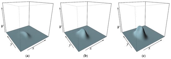
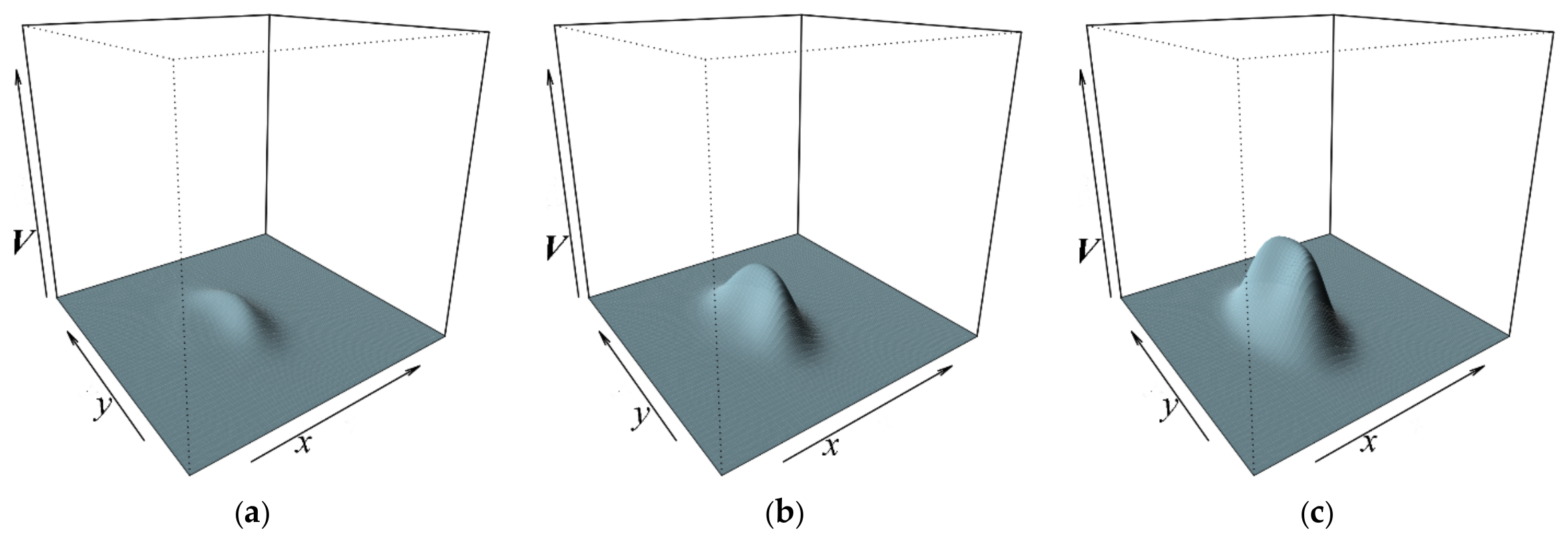
Figure 2 presents the predicted distributions of antigen concentration for the chronic form of the infectious disease [11], accounting for convection processes and diffusion perturbation ($\mathrm{\epsilon }=0.025$). The results are shown for the time $t=10$ with the administration of donor antibodies at different time points: $t_1^F=5.0$, $t_1^F=7.0$, $t_1^F=9.0$ centered at $(x_1^F,\hspace{0.33em}{y}_1^F)=(5,\hspace{0.33em}5)$ (where $G_z=\{(x,y):\hspace{0.33em}\hspace{0.33em}0\le x\le 30,\hspace{0.33em}\hspace{0.33em}0\le y\le 10\}$). The simulations indicate that earlier administration of immunological therapy produces substantially lower antigen concentrations than delayed treatment. This behavior is consistent with the ability of the immune response to suppress viral replication before large viral populations become established. The results emphasize the importance of rapid therapeutic intervention during the early stages of infection and demonstrate the sensitivity of treatment outcomes to intervention timing.

Figure 2. Distribution of antigen concentration V at time $t=10$ with the administration of donor antibodies at time points: $t_1^F=5.0$ (a); $t_1^F=7.0$ (b); $t_1^F=9.0$ (c).

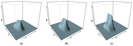
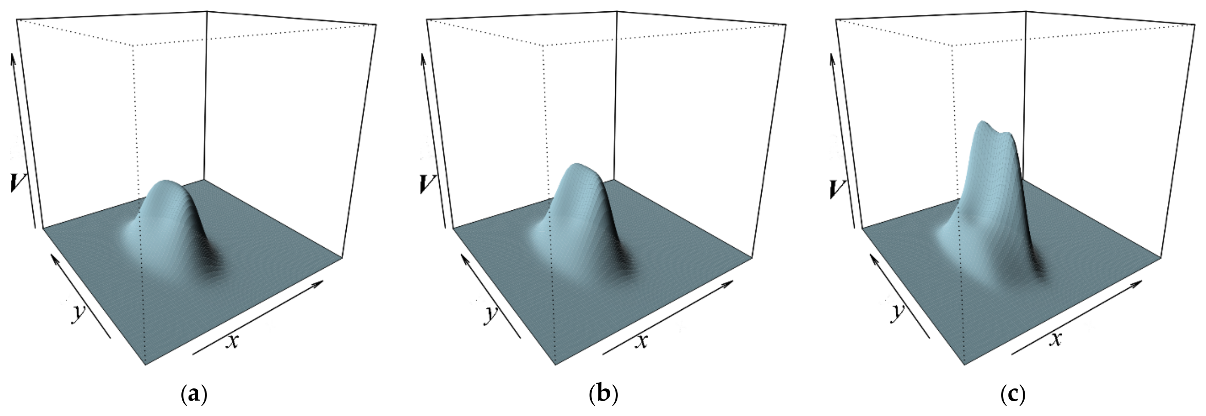
Figure 3 illustrates the predicted distributions of antigen concentration under similar conditions but for varying dosages of immunological agents. The results show that higher rates of viral particle elimination are achieved with larger administered doses. However, the use of high drug concentrations is associated with increased treatment costs and a greater risk of adverse side effects, which may place an additional burden on the patient.

Figure 3. Distribution of antigen concentration V at time $t=10$ with the administration of immunological agents of varying intensities: $A_1^F=0.0$ (a); $A_1^F=1.0$ (b); $A_1^F=2.0$ (c).

The results demonstrate that increasing the intensity of immunological therapy improves viral suppression and accelerates antigen elimination. However, the relationship is not purely beneficial. Higher treatment levels may increase treatment costs and the risk of adverse physiological effects. These simulations highlight the need to balance therapeutic effectiveness against treatment burden, supporting the development of adaptive strategies that adjust intervention intensity according to disease severity.

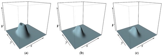
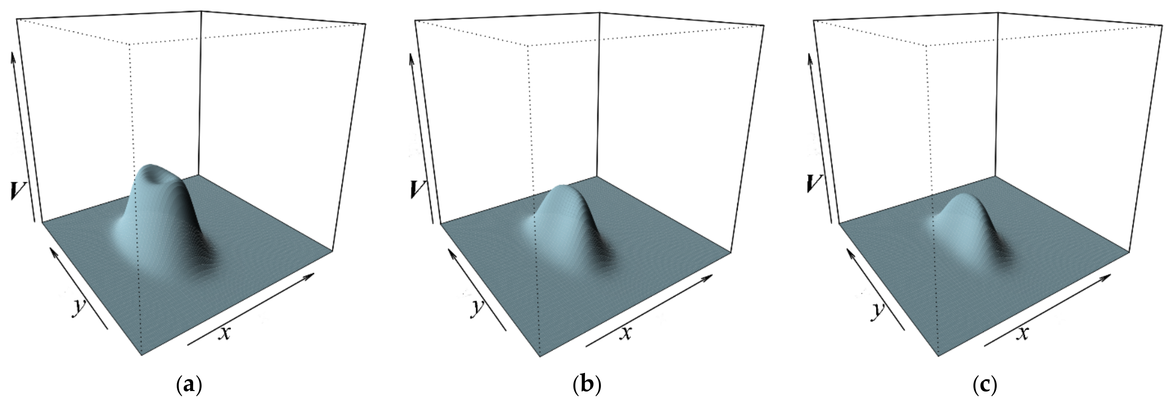
Figure 4 illustrates the influence of antipyretic therapy on infection progression. Increasing antipyretic intensity produces a more rapid reduction in body temperature; however, this temperature reduction also weakens the protective effects of the febrile response. As a consequence, viral replication may increase despite improved temperature control. These results highlight an important therapeutic trade-off: aggressive fever suppression may alleviate physiological stress while simultaneously reducing a natural defense mechanism against infection.

Figure 4. Distribution of antigen concentration V at time $t=10$ with the administration of antipyretic drugs of varying intensities: $A_1^{\mathrm{\theta }}=0.05$ (a); $A_1^{\mathrm{\theta }}=0.50$ (b); $A_1^{\mathrm{\theta }}=1.00$ (c).

These findings suggest that antipyretic therapy should be administered judiciously. Rather than eliminating fever as rapidly as possible, treatment strategies should aim to maintain temperature within a physiologically acceptable range while preserving the beneficial effects of moderate fever on infection control.

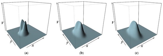
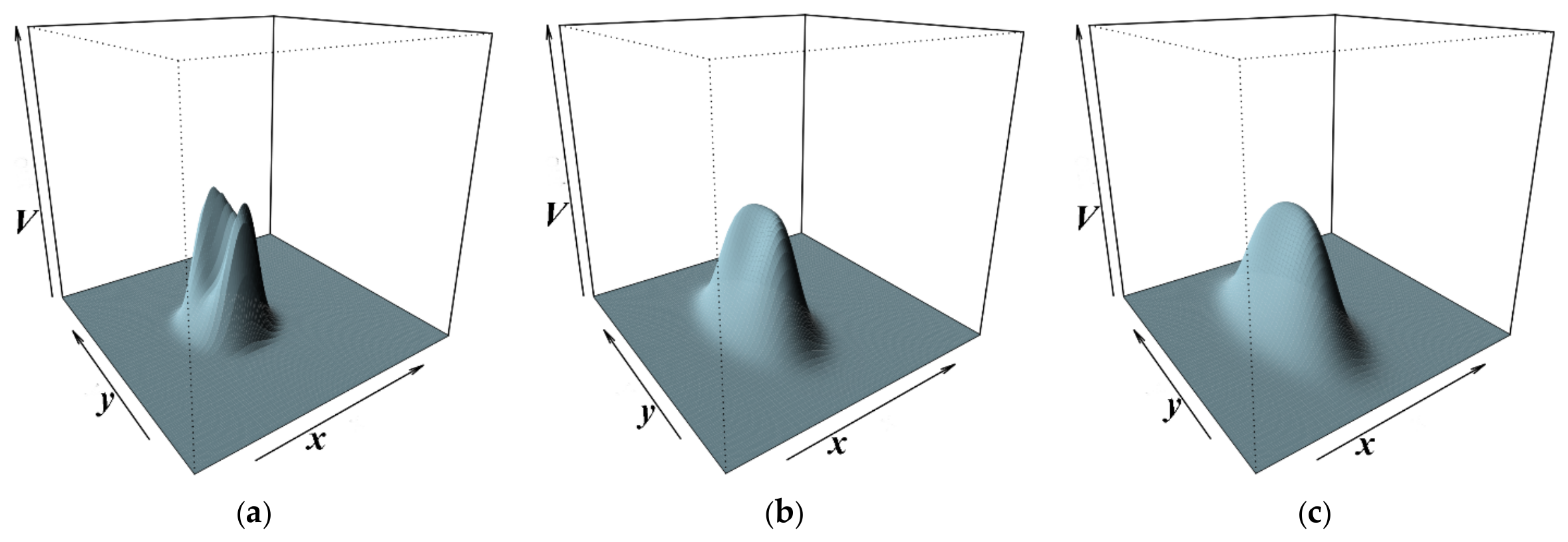
Figure 5 illustrates the influence of diffusion on the spatial evolution of infection. In the absence of diffusion, viral particles remain strongly localized near the infection focus, producing highly concentrated spatial distributions. As diffusion intensity increases, these localized structures become progressively smoother and more spatially distributed. From a biological perspective, diffusion acts as a homogenizing mechanism that reduces spatial concentration gradients and promotes the redistribution of viral particles throughout the tissue environment. These results demonstrate the importance of incorporating spatial transport processes when predicting infection dynamics and evaluating localized treatment strategies.

Figure 5. Distribution of antigen concentration V at time $t=10$ at various intensities of diffusion scattering: $\mathrm{\epsilon }=0.000$ (a); $\mathrm{\epsilon }=0.025$ (b); $\mathrm{\epsilon }=0.050$ (c).

Collectively, the numerical experiments reveal the strong interplay among therapeutic intervention, temperature regulation, and spatial transport processes. The simulations consistently indicate that treatment effectiveness depends not only on drug administration but also on the timing of intervention and the physiological environment in which the infection evolves. This observation supports the use of integrated modeling frameworks for the development of adaptive treatment protocols.

Overall, the numerical investigations demonstrate that infection dynamics are governed by the interaction of immune response, thermal regulation, spatial transport, and therapeutic intervention. Early immunological treatment improves infection control, excessive temperature suppression may compromise beneficial immune mechanisms, and diffusion significantly affects the spatial distribution of viral particles. Together, these findings provide biologically meaningful insights into treatment design and support the use of predictive mathematical models for evaluating adaptive therapeutic strategies. Although the present study is intended as a methodological investigation, the computational framework may be adapted to specific viral infections through parameter estimation using experimental or clinical data.

Although the present study focuses on methodological development, the proposed framework may be calibrated to specific viral infections using experimental or clinical data, thereby providing a foundation for predictive and patient-specific treatment analysis.

6. Conclusions

We developed a spatiotemporal model of viral infection dynamics that integrates diffusion perturbations, convection transport, temperature-dependent physiological effects, and therapeutic interventions within a unified mathematical framework. The resulting model extends classical immune-response formulations by incorporating spatial heterogeneity, delayed immune dynamics, and adaptive treatment mechanisms.

To analyze the resulting singularly perturbed delay system, we proposed a hybrid asymptotic–numerical methodology that combines the method of steps with singular perturbation techniques. This approach transforms the original problem into a sequence of computationally tractable subproblems while preserving the dominant multiscale features of the underlying dynamics. As a result, efficient approximation of the spatiotemporal evolution of infection and immune response can be achieved without direct simulation of the full system.

The numerical experiments demonstrated several biologically relevant observations. First, earlier administration of immunological therapy substantially improves infection control by reducing antigen concentrations before extensive viral proliferation occurs. Second, treatment intensity strongly influences therapeutic effectiveness, highlighting the need to balance viral suppression against treatment burden and potential adverse effects. Third, temperature regulation plays a dual role in infection dynamics. While excessive fever may have negative physiological consequences, overly aggressive antipyretic therapy may suppress beneficial fever-mediated mechanisms that contribute to infection control. Finally, diffusion processes significantly influence the spatial distribution of viral particles by reducing concentration gradients and promoting spatial redistribution throughout the tissue environment.

These findings emphasize that treatment effectiveness depends not only on the choice of therapeutic intervention but also on the timing of administration, temperature regulation, and the spatial characteristics of infection spread. The proposed framework therefore provides a useful tool for investigating the interaction between physiological regulation, immune response, and therapeutic control in spatially distributed infections.

From a methodological perspective, the study illustrates how asymptotic analysis, numerical simulation, and adaptive control can be combined within a single computational framework to address complex biological systems. The approach is sufficiently flexible to accommodate additional physiological mechanisms, treatment modalities, or disease-specific characteristics.

Future work will focus on extending the model to mixed and multi-pathogen infection scenarios, incorporating additional therapeutic strategies, and developing more rigorous optimal-control formulations. In particular, the integration of parameter-estimation procedures, data-driven calibration, and optimal-control techniques based on Pontryagin-type approaches may further improve the predictive and clinical value of the framework. The incorporation of stochastic effects and uncertainty quantification [22,23] also represents an important direction for future investigation.

Appendix A.1. Temperature-Dependent Mechanisms

The influence of temperature on viral dynamics is incorporated through functions that regulate antigen reproduction and immune response. In particular, the antigen reproduction rate is assumed to decrease with increasing temperature, while the immune system stimulation coefficient is modeled as a temperature-dependent function. The function describing the temperature effect on the recruitment of antigens is given by $\mathrm{\beta }(\mathrm{\theta })={\mathrm{\beta }}_0/(1+{\mathrm{\beta }}_1(\mathrm{\theta }-{\mathrm{\theta }}^{*}))$, leading to a decrease in production as body temperature increases. Note that ${\mathrm{\beta }}_0,\hspace{0.33em}\hspace{0.33em}{\mathrm{\beta }}_1=const>0$. We further assume that the immune system stimulation coefficient, which depends linearly on body temperature, is given by $\mathrm{\alpha }(\mathrm{\theta })={\mathrm{\alpha }}_0(1+{\mathrm{\alpha }}_1(\mathrm{\theta }-{\mathrm{\theta }}^{*}))$ where ${\mathrm{\alpha }}_0,\hspace{0.33em}\hspace{0.33em}{\mathrm{\alpha }}_1=const>0$. The baseline temperature distribution in a healthy organism is ${\mathrm{\theta }}^{*}(x,y)$

$${\mathrm{\mu }}_m(\mathrm{\theta })={\displaystyle \frac{{\mathrm{\mu }}_m^0}{1+{\mathrm{\mu }}_m^1\cdot (\mathrm{\theta }-{\mathrm{\theta }}^{*})}}, \mathrm{where} {\mathrm{\mu }}_m^1=\left\{\begin{array}{cc}0,& \mathrm{\theta }<{\mathrm{\theta }}^{**},\\ {\mathrm{\mu }}_m^{*},& \mathrm{\theta }\ge {\mathrm{\theta }}^{**},\end{array}\right.$$

A critical body temperature threshold, ${\mathrm{\theta }}^{\ast \ast }$, is introduced, above which the recovery rate of target-organ cells decreases, ${\mathrm{\mu }}_m^0,\hspace{0.33em}{\mathrm{\mu }}_m^1=const>0$; the parameters $\mathrm{\gamma }$, ${\mathrm{\mu }}_C$, $\mathrm{\tau }$, $\mathrm{\rho }$, ${\mathrm{\mu }}_f$, $\mathrm{\eta }$, $\mathrm{\sigma }$, $\mathrm{\alpha }$ (see Table A1) and the function $\mathrm{\xi }(m)$ are the same as in [11]; $\mathrm{\epsilon }{D}_V$, $\mathrm{\epsilon }{D}_F$, ${\mathrm{\epsilon }}^2{D}_C$, ${\mathrm{\epsilon }}^2{D}_m\hspace{0.17em}$, $\mathrm{\epsilon }{D}_{\mathrm{\theta }}$ are the coefficients of spatiotemporal diffusion redistribution of antigens, antibodies, plasma cells, damaged cells, and thermal conductivity, respectively; $\mathrm{\epsilon }$ is a small parameter characterizing the relatively weak influence of these diffusion effects compared to the dominant dynamics of the system.

Table A1. Parameters of the classical antiviral immune response model.

Parameter	Biological Meaning of the Parameter	Units
$\mathrm{\beta }$	Antigen reproduction rate constant	${\mathrm{day}}^{-1}$
$\mathrm{\gamma }$	Coefficient accounting for the probability of antigen–antibody encounters and the strength of their interaction	$\mathrm{ml}/\left(\mathrm{part}\cdot \mathrm{day}\right)$
$\mathrm{\alpha }$	Immune system stimulation coefficient	$\mathrm{cells}\cdot \mathrm{ml}/\left({\mathrm{part}}^2\cdot \mathrm{day}\right)$
${\mathrm{\mu }}_C$	Natural aging rate constant of plasma cells	${\mathrm{day}}^{-1}$
$\mathrm{\rho }$	Production rate constant of antibodies by a single plasma cell	${\mathrm{day}}^{-1}$
$\mathrm{\eta }$	Consumption rate constant of antibodies per unit of antigen neutralized	dimensionless
${\mathrm{\mu }}_f$	Natural decay rate constant of antibodies	${\mathrm{day}}^{-1}$
$\mathrm{\sigma }$	Destruction rate constant of target-organ cells by antigens	$\mathrm{ml}/\left(\mathrm{part}\cdot \mathrm{day}\right)$
${\mathrm{\mu }}_m$	Regeneration rate constant of the target organ	${\mathrm{day}}^{-1}$
$C^{*}$	Initial level of immunocompetent cells (plasma cells)	$\mathrm{cells}/\mathrm{ml}$
$\mathrm{\tau }$	Time required for the formation of the plasma cell cascade	$\mathrm{day}$

Table A1. Parameters of the classical antiviral immune response model.

Parameter	Biological Meaning of the Parameter	Units
$\mathrm{\beta }$	Antigen reproduction rate constant	${\mathrm{day}}^{-1}$
$\mathrm{\gamma }$	Coefficient accounting for the probability of antigen–antibody encounters and the strength of their interaction	$\mathrm{ml}/\left(\mathrm{part}\cdot \mathrm{day}\right)$
$\mathrm{\alpha }$	Immune system stimulation coefficient	$\mathrm{cells}\cdot \mathrm{ml}/\left({\mathrm{part}}^2\cdot \mathrm{day}\right)$
${\mathrm{\mu }}_C$	Natural aging rate constant of plasma cells	${\mathrm{day}}^{-1}$
$\mathrm{\rho }$	Production rate constant of antibodies by a single plasma cell	${\mathrm{day}}^{-1}$
$\mathrm{\eta }$	Consumption rate constant of antibodies per unit of antigen neutralized	dimensionless
${\mathrm{\mu }}_f$	Natural decay rate constant of antibodies	${\mathrm{day}}^{-1}$
$\mathrm{\sigma }$	Destruction rate constant of target-organ cells by antigens	$\mathrm{ml}/\left(\mathrm{part}\cdot \mathrm{day}\right)$
${\mathrm{\mu }}_m$	Regeneration rate constant of the target organ	${\mathrm{day}}^{-1}$
$C^{*}$	Initial level of immunocompetent cells (plasma cells)	$\mathrm{cells}/\mathrm{ml}$
$\mathrm{\tau }$	Time required for the formation of the plasma cell cascade	$\mathrm{day}$

Appendix A.2. Transport and Model Parameters

The model includes diffusion terms corresponding to the spatial redistribution of viral particles, immune agents, plasma cells, damaged cells, and temperature, respectively. These effects are assumed to be small and are characterized by a dimensionless parameter $ϵ$, which measures the relative strength of diffusion compared to the dominant reaction dynamics. Convection effects are described through velocity fields associated with each component, while the intercellular fluid motion is represented by a prescribed velocity field. All functions appearing in the model are assumed to be bounded and sufficiently smooth. Standard boundary conditions are imposed, with outward and inward normal directions defined on the domain boundary.

The quantities ${\mathrm{\upsilon }}^V={\mathrm{\delta }}_V\mathrm{\upsilon }=({\mathrm{\upsilon }}_x^V,{\mathrm{\upsilon }}_y^V)$, ${\mathrm{\upsilon }}^F={\mathrm{\delta }}_F\mathrm{\upsilon }=({\mathrm{\upsilon }}_x^F,{\mathrm{\upsilon }}_y^F)$, ${\mathrm{\upsilon }}^C={\mathrm{\delta }}_C\mathrm{\upsilon }=({\mathrm{\upsilon }}_x^C,{\mathrm{\upsilon }}_y^C)$, ${\mathrm{\upsilon }}^m={\mathrm{\delta }}_m\mathrm{\upsilon }=({\mathrm{\upsilon }}_x^m,{\mathrm{\upsilon }}_y^m)$, ${\mathrm{\upsilon }}^{\mathrm{\theta }}={\mathrm{\delta }}_{\mathrm{\theta }}\mathrm{\upsilon }=({\mathrm{\upsilon }}_x^{\mathrm{\theta }},{\mathrm{\upsilon }}_y^{\mathrm{\theta }})$ represent the convection transport velocities of the respective active factors of the process; $\mathrm{\upsilon }=({\mathrm{\upsilon }}_x,{\mathrm{\upsilon }}_y)$ is the velocity of the intercellular fluid. The functions $C^0(x,y)$, $m^0(x,y)$, ${\mathrm{\theta }}^0(x,y)$, $V^0(x,y,\tilde{t})$, $F^0(x,y,\tilde{t})$ are assumed to be bounded sufficiently smooth functions, $M$ is the current point of the corresponding curve and $\tilde{\mathrm{n}}$, $\mathrm{n}$ denote the outward and inward normals to the corresponding curves, respectively.

Appendix A.3. External Inputs and Therapeutic Interventions

The model incorporates localized source terms that describe abrupt changes in antigen concentration, such as the introduction of viral particles or their release from destroyed cells. Therapeutic interventions are represented through control functions corresponding to immunological and pharmacological treatments. These inputs are modeled as concentrated source terms with prescribed intensity, duration, and spatial localization The function $w^V=w^V(x,y,t)$ describes concentrated, abrupt changes in antigen concentrations [8,9]. Such changes may occur due to the entry of a concentrated dose of active viral particles into the body or their release at the sites of previously infected cell destruction. The functions $u^F=u^F(x,y,t)$ and $u^{\mathrm{\theta }}=u^{\mathrm{\theta }}(x,y,t)$ characterize the targeted impact of therapeutic agents, which provide control over the disease progression and are administered into the body via injection, etc. We represent them as point-impulse source functions with maximum values at points $(x_s^V,y_s^V)$, $(x_s^F,y_s^F)$, $(x_s^{\mathrm{\theta }},y_s^{\mathrm{\theta }})$ at time moments $t_s^V$, $t_s^F$, $t_s^{\mathrm{\theta }}$ respectively:

$$w^V(x,y,t)={\displaystyle \sum _{s=1}^{n_V}{A}_s^V\exp \left(-{\mathrm{\alpha }}_s^V\left({\left(x-x_s^V\right)}^2+{\left(y-y_s^V\right)}^2\right)\right)\cdot \exp \left(-{\mathrm{\beta }}_s^V{\left(t-t_s^V\right)}^2\right)},$$

$$u^F(x,y,t)={\displaystyle \sum _{s=1}^{n_F}{A}_s^F\exp \left(-{\mathrm{\alpha }}_s^F\left({\left(x-x_s^F\right)}^2+{\left(y-y_s^F\right)}^2\right)\right)\cdot \exp \left(-{\mathrm{\beta }}_s^F{\left(t-t_s^F\right)}^2\right)},$$

$$u^{\mathrm{\theta }}(x,y,t)={\displaystyle \sum _{s=1}^{n_{\mathrm{\theta }}}{A}_s^{\mathrm{\theta }}\exp \left(-{\mathrm{\alpha }}_s^{\mathrm{\theta }}\left({\left(x-x_s^{\mathrm{\theta }}\right)}^2+{\left(y-y_s^{\mathrm{\theta }}\right)}^2\right)\right)\cdot \exp \left(-{\mathrm{\beta }}_s^{\mathrm{\theta }}{\left(t-t_s^{\mathrm{\theta }}\right)}^2\right)}.$$

where $A_s^V$, $A_s^F$, $A_s^{\mathrm{\theta }}$, ${\mathrm{\alpha }}_s^V$, ${\mathrm{\alpha }}_s^F$, ${\mathrm{\alpha }}_s^{\mathrm{\theta }}$, ${\mathrm{\beta }}_s^V$, ${\mathrm{\beta }}_s^F$, ${\mathrm{\beta }}_s^{\mathrm{\theta }}$ are parameters that determine the intensity, duration, and spatial extent of the corresponding concentrated interventions [8,9]. To predict the progression of a viral infection in a scenario involving the administration of injectable solutions via an intravenous drip at points $(x_s^F,y_s^F)$ over time intervals $({\overline{t}}_s^F,{\overline{\overline{t}}}_s^F)$, the corresponding function $u^F(x,y,t)$ is

$$u^F(x,y,t)={\displaystyle \sum _{s=1}^{n_F}{A}_s^F\exp \left(-{\mathrm{\alpha }}_s^F\left({\left(x-x_s^F\right)}^2+{\left(y-y_s^F\right)}^2\right)\right)\cdot \left[\frac{\exp \left(-{\mathrm{\beta }}_s^F{\left(t-{\overline{t}}_s^F\right)}^2\right)}{1+\exp \left(-{\mathrm{\beta }}_s^F{\left(t-{\overline{t}}_s^F\right)}^2\right)}-\frac{\exp \left(-{\mathrm{\beta }}_s^F{\left(t-{\overline{\overline{t}}}_s^F\right)}^2\right)}{1+\exp \left(-{\mathrm{\beta }}_s^F{\left(t-{\overline{\overline{t}}}_s^F\right)}^2\right)}\right]}.$$

Appendix A.4. Asymptotic Expansion Structure

The solutions to the singularly perturbed problems are constructed in the form of asymptotic expansions:

$$\begin{array}{c}{V}_{(k)}={\displaystyle {\displaystyle \sum _{i=0}^n}{\mathrm{\epsilon }}^i{V}_{(k,i)}}+{\displaystyle {\displaystyle \sum _{i=0}^n}{\mathrm{\epsilon }}^i{\Pi }_{(k,i)}^V}+{\displaystyle {\displaystyle \sum _{i=0}^{2n}}{\mathrm{\epsilon }}^{\frac{i}{2}}{\mathrm{{\rm P}}}_{(k,\frac{i}{2})}^V}+{\displaystyle {\displaystyle \sum _{i=0}^{2n}}{\mathrm{\epsilon }}^{\frac{i}{2}}{\overline{\mathrm{{\rm P}}}}_{(k,\frac{i}{2})}^V}+R_{(k,n)}^V,\\ C_{(k)}={\displaystyle {\displaystyle \sum _{i=0}^n}{\mathrm{\epsilon }}^i{C}_{(k,i)}}+{\displaystyle {\displaystyle \sum _{i=0}^n}{\mathrm{\epsilon }}^i{\Pi }_{(k,i)}^C}+{\displaystyle {\displaystyle \sum _{i=0}^{2n}}{\mathrm{\epsilon }}^{\frac{i}{2}}{\mathrm{{\rm P}}}_{(k,\frac{i}{2})}^C}+{\displaystyle {\displaystyle \sum _{i=0}^{2n}}{\mathrm{\epsilon }}^{\frac{i}{2}}{\overline{\mathrm{{\rm P}}}}_{(k,\frac{i}{2})}^C}+R_{(k,n)}^C,\\ F_{(k)}={\displaystyle {\displaystyle \sum _{i=0}^n}{\mathrm{\epsilon }}^i{F}_{(k,i)}}+{\displaystyle {\displaystyle \sum _{i=0}^n}{\mathrm{\epsilon }}^i{\Pi }_{(k,i)}^F}+{\displaystyle {\displaystyle \sum _{i=0}^{2n}}{\mathrm{\epsilon }}^{\frac{i}{2}}{\mathrm{{\rm P}}}_{(k,\frac{i}{2})}^F}+{\displaystyle {\displaystyle \sum _{i=0}^{2n}}{\mathrm{\epsilon }}^{\frac{i}{2}}{\overline{\mathrm{{\rm P}}}}_{(k,\frac{i}{2})}^F}+R_{(k,n)}^F,\\ m_{(k)}={\displaystyle {\displaystyle \sum _{i=0}^n}{\mathrm{\epsilon }}^i{m}_{(k,i)}}+{\displaystyle {\displaystyle \sum _{i=0}^n}{\mathrm{\epsilon }}^i{\Pi }_{(k,i)}^m}+{\displaystyle {\displaystyle \sum _{i=0}^{2n}}{\mathrm{\epsilon }}^{\frac{i}{2}}{\mathrm{{\rm P}}}_{(k,\frac{i}{2})}^m}+{\displaystyle {\displaystyle \sum _{i=0}^{2n}}{\mathrm{\epsilon }}^{\frac{i}{2}}{\overline{\mathrm{{\rm P}}}}_{(k,\frac{i}{2})}^m}+R_{(k,n)}^m,\\ {\mathrm{\theta }}_{(k)}={\displaystyle {\displaystyle \sum _{i=0}^n}{\mathrm{\epsilon }}^i{\mathrm{\theta }}_{(k,i)}}+{\displaystyle {\displaystyle \sum _{i=0}^n}{\mathrm{\epsilon }}^i{\Pi }_{(k,i)}^{\mathrm{\theta }}}+{\displaystyle {\displaystyle \sum _{i=0}^{2n}}{\mathrm{\epsilon }}^{\frac{i}{2}}{\mathrm{{\rm P}}}_{(k,\frac{i}{2})}^{\mathrm{\theta }}}+{\displaystyle {\displaystyle \sum _{i=0}^{2n}}{\mathrm{\epsilon }}^{\frac{i}{2}}{\overline{\mathrm{{\rm P}}}}_{(k,\frac{i}{2})}^{\mathrm{\theta }}}+R_{(k,n)}^{\mathrm{\theta }},\end{array}$$

constructed as perturbations of the solutions to the associated degenerate problems [6,7,8,9]. Here, $k=0,1,2,\dots$, $V_{(k,i)}=V_{(k,i)}(\mathrm{\phi },\mathrm{\psi },t)$, $C_{(k,i)}=C_{(k,i)}(\mathrm{\phi },\mathrm{\psi },t)$, $F_{(k,i)}=F_{(k,i)}(\mathrm{\phi },\mathrm{\psi },t)$, $m_{(k,i)}=m_{(k,i)}(\mathrm{\phi },\mathrm{\psi },t)$, ${\mathrm{\theta }}_{(k,i)}={\mathrm{\theta }}_{(k,i)}(\mathrm{\phi },\mathrm{\psi },t)$ denote the unknown functions corresponding to the regular (outer) part of the asymptotic expansion, while ${\Pi }_{(k,i)}^V={\Pi }_{(k,i)}^V(\mathrm{\eta },\mathrm{\psi },t)$, ${\Pi }_{(k,i)}^C={\Pi }_{(k,i)}^C(\mathrm{\eta },\mathrm{\psi },t)$, ${\Pi }_{(k,i)}^F={\Pi }_{(k,i)}^F(\mathrm{\eta },\mathrm{\psi },t)$, ${\Pi }_{(k,i)}^m={\Pi }_{(k,i)}^m(\mathrm{\eta },\mathrm{\psi },t)$, ${\Pi }_{(k,i)}^{\mathrm{\theta }}={\Pi }_{(k,i)}^{\mathrm{\theta }}(\mathrm{\eta },\mathrm{\psi },t)$ represent the boundary layer corrections in the neighborhoods of the corresponding spatial boundaries. Additional boundary layer functions in the neighborhood of $\mathrm{\phi }={\mathrm{\phi }}^{\ast }$. The functions ${\mathrm{{\rm P}}}_{(k,\frac{i}{2})}^V={\mathrm{{\rm P}}}_{(k,\frac{i}{2})}^V(\mathrm{\phi },\mathrm{\xi },t)$, ${\mathrm{{\rm P}}}_{(k,\frac{i}{2})}^C={\mathrm{{\rm P}}}_{(k,\frac{i}{2})}^C(\mathrm{\phi },\mathrm{\xi },t)$, ${\mathrm{{\rm P}}}_{(k,\frac{i}{2})}^F={\mathrm{{\rm P}}}_{(k,\frac{i}{2})}^F(\mathrm{\phi },\mathrm{\xi },t)$, ${\mathrm{{\rm P}}}_{(k,\frac{i}{2})}^m={\mathrm{{\rm P}}}_{(k,\frac{i}{2})}^m(\mathrm{\phi },\mathrm{\xi },t)$, ${\mathrm{{\rm P}}}_{(k,\frac{i}{2})}^{\mathrm{\theta }}={\mathrm{{\rm P}}}_{(k,\frac{i}{2})}^{\mathrm{\theta }}(\mathrm{\phi },\mathrm{\xi },t)$, ${\overline{\mathrm{{\rm P}}}}_{(k,\frac{i}{2})}^V={\overline{\mathrm{{\rm P}}}}_{(k,\frac{i}{2})}^V(\mathrm{\phi },\mathrm{\zeta },t)$, ${\mathrm{{\rm P}}}_{(k,\frac{i}{2})}^C={\overline{\mathrm{{\rm P}}}}_{(k,\frac{i}{2})}^C(\mathrm{\phi },\mathrm{\zeta },t)$, ${\overline{\mathrm{{\rm P}}}}_{(k,\frac{i}{2})}^F={\overline{\mathrm{{\rm P}}}}_{(k,\frac{i}{2})}^F(\mathrm{\phi },\mathrm{\zeta },t)$, ${\overline{\mathrm{{\rm P}}}}_{(k,\frac{i}{2})}^m={\overline{\mathrm{{\rm P}}}}_{(k,\frac{i}{2})}^m(\mathrm{\phi },\mathrm{\zeta },t)$, ${\overline{\mathrm{{\rm P}}}}_{(k,\frac{i}{2})}^{\mathrm{\theta }}={\overline{\mathrm{{\rm P}}}}_{(k,\frac{i}{2})}^{\mathrm{\theta }}(\mathrm{\phi },\mathrm{\zeta },t)$ are introduced in the vicinity of $\mathrm{\psi }=0$ and $\mathrm{\psi }=Q$ respectively. The functions $\mathrm{\eta }=({\mathrm{\phi }}^{\ast }-\mathrm{\phi }){\mathrm{\epsilon }}^{-1}$, $\mathrm{\xi }=\mathrm{\psi }{\mathrm{\epsilon }}^{-1/2}$, $\mathrm{\zeta }=(Q-\mathrm{\psi }){\mathrm{\epsilon }}^{-1/2}$ are the corresponding regularizing transformations [19], and $R_{(k,n)}^V=R_{(k,n)}^V(\mathrm{\phi },\mathrm{\psi },t,\mathrm{\epsilon })$, $R_{(k,n)}^C=R_{(k,n)}^C(\mathrm{\phi },\mathrm{\psi },t,\mathrm{\epsilon })$, $R_{(k,n)}^F=R_{(k,n)}^F(\mathrm{\phi },\mathrm{\psi },t,\mathrm{\epsilon })$, $R_{(k,n)}^m=R_{(k,n)}^m(\mathrm{\phi },\mathrm{\psi },t,\mathrm{\epsilon })$, $R_{(k,n)}^{\mathrm{\theta }}=R_{(k,n)}^{\mathrm{\theta }}(\mathrm{\phi },\mathrm{\psi },t,\mathrm{\epsilon })$ are the corresponding residual terms.

The governing equations for the unknown functions $V_{(k,i)}(x,y,t)$, $C_{(k,i)}(x,y,t)$, $F_{(k,i)}(x,y,t)$, $m_{(k,i)}(x,y,t)$, ${\mathrm{\theta }}_{(k,i)}(x,y,t)$ are obtained by applying the standard procedure of equating coefficients of like powers of the small parameter [19]. In the case where $\mathrm{\xi }(m_{(k,0)})=1$ (i.e., when the level of target organ damage does not reduce the antibody production rate), the associated simplified (degenerate) problem for determining $V_{(k,0)}$, $C_{(k,0)}$, $F_{(k,0)}$, $m_{(k,0)}$, ${\mathrm{\theta }}_{(k,0)}$:

$$\begin{array}{c}{\displaystyle \frac{\partial V_{(k,0)}}{\partial t}}=w_{(k)}^V+B_0{V}_{(k,0)}-\mathrm{\gamma }{F}_{(k,0)}{V}_{(k,0)}-{\mathrm{\delta }}_V{\mathrm{\upsilon }}^2(\mathrm{\phi },\mathrm{\psi }){\displaystyle \frac{\partial V_{(k,0)}}{\partial \mathrm{\phi }}},\\ {\displaystyle \frac{\partial C_{(k,0)}}{\partial t}}={\mathrm{\alpha }}_0\left(1+{\mathrm{\alpha }}_1\left({\mathrm{\theta }}_{(k,0)}-{\mathrm{\theta }}^{*}\right)\right){\mathrm{\Psi }}_{(k)}-{\mathrm{\mu }}_C\cdot \left(C_{(k,0)}-C^{\ast }\right)-{\mathrm{\delta }}_C{\mathrm{\upsilon }}^2(\mathrm{\phi },\mathrm{\psi }){\displaystyle \frac{\partial C_{(k,0)}}{\partial \mathrm{\phi }}},\\ {\displaystyle \frac{\partial F_{(k,0)}}{\partial t}}=u_{(k)}^F+\mathrm{\rho }{C}_{(k,0)}-{\mathrm{\mu }}_f{F}_{(k,0)}-\mathrm{\eta }\mathrm{\gamma }{V}_{(k,0)}{F}_{(k,0)}-{\mathrm{\delta }}_F{\mathrm{\upsilon }}^2(\mathrm{\phi },\mathrm{\psi }){\displaystyle \frac{\partial F_{(k,0)}}{\partial \mathrm{\phi }}},\\ {\displaystyle \frac{\partial m_{(k,0)}}{\partial t}}=\mathrm{\sigma }{V}_{(k,0)}-M_0{m}_{(k,0)}-{\mathrm{\delta }}_m{\mathrm{\upsilon }}^2(\mathrm{\phi },\mathrm{\psi }){\displaystyle \frac{\partial m_{(k,0)}}{\partial \mathrm{\phi }}},\\ {\displaystyle \frac{\partial {\mathrm{\theta }}_{(k,0)}}{\partial t}}={\mathrm{\alpha }}_{\mathrm{\theta }}{F}_{(k,0)}{V}_{(k,0)}-{\mathrm{\mu }}_{\mathrm{\theta }}\cdot \left({\mathrm{\theta }}_{(k,0)}-{\mathrm{\theta }}^{*}\right)-{\mathrm{\lambda }}_{\mathrm{\theta }}\cdot u_{(k)}^{\mathrm{\theta }}-{\mathrm{\delta }}_{\mathrm{\theta }}{\mathrm{\upsilon }}^2(\mathrm{\phi },\mathrm{\psi }){\displaystyle \frac{\partial {\mathrm{\theta }}_{(k,0)}}{\partial \mathrm{\phi }}};\\ C_{(k,0)}(\mathrm{\phi },\mathrm{\psi },k\mathrm{\tau })=C_{(k-1)}(\mathrm{\phi },\mathrm{\psi },k\mathrm{\tau }),\hspace{0.33em}\hspace{0.33em}{m}_{(k,0)}(\mathrm{\phi },\mathrm{\psi },k\mathrm{\tau })=m_{(k-1)}(\mathrm{\phi },\mathrm{\psi },k\mathrm{\tau }),\\ {\mathrm{\theta }}_{(k,0)}(\mathrm{\phi },\mathrm{\psi },k\mathrm{\tau })={\mathrm{\theta }}_{(k-1)}(\mathrm{\phi },\mathrm{\psi },k\mathrm{\tau }),\hspace{0.33em}\hspace{0.33em}{V}_{(k,0)}(\mathrm{\phi },\mathrm{\psi },k\mathrm{\tau })=V_{(k-1)}(\mathrm{\phi },\mathrm{\psi },k\mathrm{\tau }),\\ F_{(k,0)}(\mathrm{\phi },\mathrm{\psi },k\mathrm{\tau })=F_{(k-1)}(\mathrm{\phi },\mathrm{\psi },k\mathrm{\tau }),\hspace{0.33em}\hspace{0.33em}{V}_{(k,0)}{\mathrm{|}}_{AB}=V_{\ast }(\mathrm{\psi },t),\hspace{0.33em}\hspace{0.33em}{F}_{(k,0)}{\mathrm{|}}_{AB}=F_{\ast }(\mathrm{\psi },t),\\ C_{(k,0)}{\mathrm{|}}_{AB}=C_{\ast }(\mathrm{\psi },t),\hspace{0.33em}\hspace{0.33em}{m}_{(k,0)}{\mathrm{|}}_{AB}=m_{\ast }(\mathrm{\psi },t),\hspace{0.33em}\hspace{0.33em}{\mathrm{\theta }}_{(k,0)}{\mathrm{|}}_{AB}={\mathrm{\theta }}_{\ast }(\mathrm{\psi },t);\end{array}$$

(A1)

$$\begin{array}{c}{\displaystyle \frac{\partial V_{(k,i)}}{\partial t}}=\left(B_0{V}_{(k,i)}+B_i{V}_{(k,0)}\right)-\mathrm{\gamma }\left(a_{(k,0)}{F}_{(k,i)}+b_{(k,0)}{V}_{(k,i)}\right)-{\mathrm{\delta }}_V{\mathrm{\upsilon }}^2(\mathrm{\phi },\mathrm{\psi }){\displaystyle \frac{\partial V_{(k,i)}}{\partial \mathrm{\phi }}}+{\mathrm{\Phi }}_i^V,\\ {\displaystyle \frac{\partial C_{(k,i)}}{\partial t}}={\mathrm{\alpha }}_0{\mathrm{\alpha }}_1{\mathrm{\theta }}_{(k,i)}{\mathrm{\Psi }}_{(k)}-{\mathrm{\mu }}_C{C}_{(k,i)}-{\mathrm{\delta }}_C{\mathrm{\upsilon }}^2(\mathrm{\phi },\mathrm{\psi }){\displaystyle \frac{\partial C_{(k,i)}}{\partial \mathrm{\phi }}}+{\mathrm{\Phi }}_i^C,\\ {\displaystyle \frac{\partial F_{(k,i)}}{\partial t}}=\mathrm{\rho }{C}_{(k,i)}-{\mathrm{\mu }}_f{F}_{(k,i)}-\mathrm{\eta }\mathrm{\gamma }\left(a_{(k,0)}{F}_{(k,i)}+b_{(k,0)}{V}_{(k,i)}\right)-{\mathrm{\delta }}_F{\mathrm{\upsilon }}^2(\mathrm{\phi },\mathrm{\psi }){\displaystyle \frac{\partial F_{(k,i)}}{\partial \mathrm{\phi }}}+{\mathrm{\Phi }}_i^F,\\ {\displaystyle \frac{\partial m_{(k,i)}}{\partial t}}=\mathrm{\sigma }{V}_{(k,i)}-\left(M_0{m}_{(k,i)}+M_i{m}_{(k,0)}\right)-{\mathrm{\delta }}_m{\mathrm{\upsilon }}^2(\mathrm{\phi },\mathrm{\psi }){\displaystyle \frac{\partial m_{(k,i)}}{\partial \mathrm{\phi }}}+{\mathrm{\Phi }}_i^m,\\ {\displaystyle \frac{\partial {\mathrm{\theta }}_{(k,i)}}{\partial t}}={\mathrm{\alpha }}_{\mathrm{\theta }}\left(a_{(k,0)}{F}_{(k,i)}+b_{(k,0)}{V}_{(k,i)}\right)-{\mathrm{\mu }}_{\mathrm{\theta }}{V}_{(k,i)}-{\mathrm{\delta }}_{\mathrm{\theta }}{\mathrm{\upsilon }}^2(\mathrm{\phi },\mathrm{\psi }){\displaystyle \frac{\partial {\mathrm{\theta }}_{(k,i)}}{\partial \mathrm{\phi }}}+{\mathrm{\Phi }}_i^{\mathrm{\theta }};\\ C_{(k,i)}(\mathrm{\phi },\mathrm{\psi },k\mathrm{\tau })=0,\hspace{0.33em}\hspace{0.33em}{m}_{(k,i)}(\mathrm{\phi },\mathrm{\psi },k\mathrm{\tau })=0,\hspace{0.33em}\hspace{0.33em}{\mathrm{\theta }}_{(k,i)}(\mathrm{\phi },\mathrm{\psi },k\mathrm{\tau })=0,\hspace{0.33em}\hspace{0.33em}{V}_{(k,i)}(\mathrm{\phi },\mathrm{\psi },k\mathrm{\tau })=0,\\ F_{(k,i)}(\mathrm{\phi },\mathrm{\psi },k\mathrm{\tau })=0,\hspace{0.33em}\hspace{0.33em}{V}_{(k,i)}{\mathrm{|}}_{AB}=0,\hspace{0.33em}\hspace{0.33em}{F}_{(k,i)}{\mathrm{|}}_{AB}=0,\hspace{0.33em}\hspace{0.33em}{C}_{(k,i)}{\mathrm{|}}_{AB}=0,\hspace{0.33em}\hspace{0.33em}{m}_{(k,i)}{\mathrm{|}}_{AB}=0,\\ {\mathrm{\theta }}_{(k,i)}{\mathrm{|}}_{AB}=0,\hspace{0.33em}\hspace{0.33em}i=2,3,\dots ,n\hspace{0.17em};\end{array}$$

(A2)

where $a_{(k,0)}=V_{(k,0)}$, $b_{(k,0)}=F_{(k,0)}$, $B_0={\displaystyle \frac{{\mathrm{\beta }}_0}{1+{\mathrm{\beta }}_1\cdot ({\mathrm{\theta }}_{(k,0)}-{\mathrm{\theta }}^{*})}}$, $B_i=-{\displaystyle \frac{{\mathrm{\beta }}_1\cdot {\displaystyle \sum _{j=0}^{i-1}{\mathrm{\theta }}_{(k,i-j)}{B}_j}}{1+{\mathrm{\beta }}_1\cdot ({\mathrm{\theta }}_{(k,0)}-{\mathrm{\theta }}^{*})}}$, $M_0={\displaystyle \frac{{\mathrm{\mu }}_m^0}{1+{\mathrm{\mu }}_m^1\cdot ({\mathrm{\theta }}_0-{\mathrm{\theta }}^{*})}}$, $M_i=-{\displaystyle \frac{{\mathrm{\mu }}_m^1\cdot {\displaystyle \sum _{j=0}^{i-1}{\mathrm{\theta }}_{i-j}{M}_j}}{1+{\mathrm{\mu }}_m^1\cdot ({\mathrm{\theta }}_0-{\mathrm{\theta }}^{*})}}$, ${\mathrm{\Phi }}_1^V=D_V{\mathrm{\upsilon }}^2(\mathrm{\phi },\mathrm{\psi })\left({\displaystyle \frac{{\partial }^2{V}_{(k,0)}}{\partial {\mathrm{\phi }}^2}}+{\displaystyle \frac{{\partial }^2{V}_{(k,0)}}{\partial {\mathrm{\psi }}^2}}\right)$, ${\mathrm{\Phi }}_1^C=D_C{\mathrm{\upsilon }}^2(\mathrm{\phi },\mathrm{\psi })\left({\displaystyle \frac{{\partial }^2{C}_{(k,0)}}{\partial {\mathrm{\phi }}^2}}+{\displaystyle \frac{{\partial }^2{C}_{(k,0)}}{\partial {\mathrm{\psi }}^2}}\right)$, ${\mathrm{\Phi }}_1^m=D_m{\mathrm{\upsilon }}^2(\mathrm{\phi },\mathrm{\psi })\left({\displaystyle \frac{{\partial }^2{m}_{(k,0)}}{\partial {\mathrm{\phi }}^2}}+{\displaystyle \frac{{\partial }^2{m}_{(k,0)}}{\partial {\mathrm{\psi }}^2}}\right)$, ${\mathrm{\Phi }}_1^F=D_F{\mathrm{\upsilon }}^2(\mathrm{\phi },\mathrm{\psi })\left({\displaystyle \frac{{\partial }^2{F}_{(k,0)}}{\partial {\mathrm{\phi }}^2}}+{\displaystyle \frac{{\partial }^2{F}_{(k,0)}}{\partial {\mathrm{\psi }}^2}}\right)$, ${\mathrm{\Phi }}_1^{\mathrm{\theta }}=D_{\mathrm{\theta }}{\mathrm{\upsilon }}^2(\mathrm{\phi },\mathrm{\psi })\times$ $\times \left({\displaystyle \frac{{\partial }^2{\mathrm{\theta }}_{(k,0)}}{\partial {\mathrm{\phi }}^2}}+{\displaystyle \frac{{\partial }^2{\mathrm{\theta }}_{(k,0)}}{\partial {\mathrm{\psi }}^2}}\right)$, ${\mathrm{\Phi }}_i^V={\displaystyle {\displaystyle \sum _{j=1}^{i-1}}{B}_j{V}_{(k,i-j)}}-\mathrm{\gamma }{\displaystyle {\displaystyle \sum _{j=1}^{i-1}}{V}_{(k,j)}{F}_{(k,i-j)}}+D_V{\mathrm{\upsilon }}^2(\mathrm{\phi },\mathrm{\psi })\left({\displaystyle \frac{{\partial }^2{V}_{(k,i-1)}}{\partial {\mathrm{\phi }}^2}}+{\displaystyle \frac{{\partial }^2{V}_{(k,i-1)}}{\partial {\mathrm{\psi }}^2}}\right)$, ${\mathrm{\Phi }}_i^C=D_C\times$ $\times {\mathrm{\upsilon }}^2(\mathrm{\phi },\mathrm{\psi })\left({\displaystyle \frac{{\partial }^2{C}_{(k,i-1)}}{\partial {\mathrm{\phi }}^2}}+{\displaystyle \frac{{\partial }^2{C}_{(k,i-1)}}{\partial {\mathrm{\psi }}^2}}\right)$, ${\mathrm{\Phi }}_i^F=-\mathrm{\eta }\mathrm{\gamma }{\displaystyle \sum _{j=1}^{i-1}{V}_{(k,j)}{F}_{(k,i-j)}}+D_F{\mathrm{\upsilon }}^2(\mathrm{\phi },\mathrm{\psi })\left({\displaystyle \frac{{\partial }^2{F}_{(k,i-1)}}{\partial {\mathrm{\phi }}^2}}+{\displaystyle \frac{{\partial }^2{F}_{(k,i-1)}}{\partial {\mathrm{\psi }}^2}}\right)$, ${\mathrm{\Phi }}_i^m=D_m{\mathrm{\upsilon }}^2(\mathrm{\phi },\mathrm{\psi })\left({\displaystyle \frac{{\partial }^2{m}_{(k,i-1)}}{\partial {\mathrm{\phi }}^2}}+{\displaystyle \frac{{\partial }^2{m}_{(k,i-1)}}{\partial {\mathrm{\psi }}^2}}\right)-{\displaystyle \sum _{j=1}^{i-1}{M}_j{m}_{(k,i-j)}}$, ${\mathrm{\Phi }}_i^{\mathrm{\theta }}={\mathrm{\alpha }}_{\mathrm{\theta }}{\displaystyle \sum _{j=1}^{i-1}{V}_{(k,j)}{F}_{(k,i-j)}}+D_{\mathrm{\theta }}{\mathrm{\upsilon }}^2(\mathrm{\phi },\mathrm{\psi })\left({\displaystyle \frac{{\partial }^2{\mathrm{\theta }}_{(k,i-1)}}{\partial {\mathrm{\phi }}^2}}\right.\left.+{\displaystyle \frac{{\partial }^2{\mathrm{\theta }}_{(k,i-1)}}{\partial {\mathrm{\psi }}^2}}\right)$.

Appendix A.5. Degenerate and Correction Problems

For example, the following problems are obtained to find the functions ${\mathrm{{\rm P}}}_{(k,\frac{i}{2})}^V$, ${\mathrm{{\rm P}}}_{(k,\frac{i}{2})}^C$, ${\mathrm{{\rm P}}}_{(k,\frac{i}{2})}^F$, ${\mathrm{{\rm P}}}_{(k,\frac{i}{2})}^m$, ${\mathrm{{\rm P}}}_{(k,\frac{i}{2})}^{\mathrm{\theta }}$:

$$\begin{array}{c}{\displaystyle \frac{\partial {\mathrm{P}}_{(k,0)}^V}{\partial t}}+{\mathrm{\delta }}_V{\mathrm{\upsilon }}^2(\mathrm{\phi },\mathrm{\xi }){\displaystyle \frac{\partial {\mathrm{P}}_{(k,0)}^V}{\partial \mathrm{\phi }}}-D_V{\mathrm{\upsilon }}^2(\mathrm{\phi },\mathrm{\xi }){\displaystyle \frac{{\partial }^2{\mathrm{P}}_{(k,0)}^V}{\partial {\mathrm{\xi }}^2}}={\mathrm{{\rm B}}}_{(0)}^P{V}_{(k)}^{reg}+\left(\mathrm{\beta }({\mathrm{\theta }}_{(k)}^{reg})+{\mathrm{{\rm B}}}_{(0)}^P\right)\cdot {\mathrm{{\rm P}}}_{(k,0)}^V-\mathrm{\gamma }{V}_{(k)}^{reg}{\mathrm{P}}_{(k,0)}^F-\\ -\mathrm{\gamma }{F}_{(k)}^{reg}{\mathrm{P}}_{(k,0)}^V-\mathrm{\gamma }{\mathrm{P}}_{(k,0)}^V{\mathrm{P}}_{(k,0)}^F,\\ {\displaystyle \frac{\partial {\mathrm{P}}_{(k,0)}^C}{\partial t}}+{\mathrm{\delta }}_C{\mathrm{\upsilon }}^2(\mathrm{\phi },\mathrm{\xi }){\displaystyle \frac{\partial {\mathrm{P}}_{(k,0)}^C}{\partial \mathrm{\phi }}}-D_C{\mathrm{\upsilon }}^2(\mathrm{\phi },\mathrm{\xi }){\displaystyle \frac{{\partial }^2{\mathrm{P}}_{(k,0)}^C}{\partial {\mathrm{\xi }}^2}}=-{\mathrm{\mu }}_C{\mathrm{P}}_{(k,0)}^C,\\ {\displaystyle \frac{\partial {\mathrm{P}}_{(k,0)}^F}{\partial t}}+{\mathrm{\delta }}_F{\mathrm{\upsilon }}^2(\mathrm{\phi },\mathrm{\xi }){\displaystyle \frac{\partial {\mathrm{P}}_{(k,0)}^F}{\partial \mathrm{\phi }}}-D_F{\mathrm{\upsilon }}^2(\mathrm{\phi },\mathrm{\xi }){\displaystyle \frac{{\partial }^2{\mathrm{P}}_{(k,0)}^F}{\partial {\mathrm{\xi }}^2}}=\mathrm{\rho }{\mathrm{P}}_{(k,0)}^C-{\mathrm{\mu }}_f{\mathrm{P}}_{(k,0)}^F-\mathrm{\eta }\mathrm{\gamma }{V}_{(k)}^{reg}{\mathrm{P}}_{(k,0)}^F-\\ -\mathrm{\eta }\mathrm{\gamma }{F}_{(k)}^{reg}{\mathrm{P}}_{(k,0)}^V-\mathrm{\eta }\mathrm{\gamma }{\mathrm{P}}_{(k,0)}^V{\mathrm{P}}_{(k,0)}^F,\\ {\displaystyle \frac{\partial {\mathrm{P}}_{(k,0)}^m}{\partial t}}+{\mathrm{\delta }}_m{\mathrm{\upsilon }}^2(\mathrm{\phi },\mathrm{\xi }){\displaystyle \frac{\partial {\mathrm{P}}_{(k,0)}^m}{\partial \mathrm{\phi }}}-D_m{\mathrm{\upsilon }}^2(\mathrm{\phi },\mathrm{\xi }){\displaystyle \frac{{\partial }^2{\mathrm{P}}_{(k,0)}^m}{\partial {\mathrm{\xi }}^2}}=\mathrm{\sigma }{\mathrm{P}}_{(k,0)}^V-M_{(0)}^P{m}_{(k)}^{reg}-\left({\mathrm{\mu }}_m({\mathrm{\theta }}_{(k)}^{reg})+M_{(0)}^P\right)\cdot {\mathrm{{\rm P}}}_{(k,0)}^m,\\ {\displaystyle \frac{\partial {\mathrm{P}}_{(k,0)}^{\mathrm{\theta }}}{\partial t}}+{\mathrm{\delta }}_{\mathrm{\theta }}{\mathrm{\upsilon }}^2(\mathrm{\phi },\mathrm{\xi }){\displaystyle \frac{\partial {\mathrm{P}}_{(k,0)}^{\mathrm{\theta }}}{\partial \mathrm{\phi }}}-D_{\mathrm{\theta }}{\mathrm{\upsilon }}^2(\mathrm{\phi },\mathrm{\xi }){\displaystyle \frac{{\partial }^2{\mathrm{P}}_{(k,0)}^{\mathrm{\theta }}}{\partial {\mathrm{\xi }}^2}}={\mathrm{\alpha }}_{\mathrm{\theta }}{V}_{(k)}^{reg}{\mathrm{P}}_{(k,0)}^F+{\mathrm{\alpha }}_{\mathrm{\theta }}{F}_{(k)}^{reg}{\mathrm{P}}_{(k,0)}^V+{\mathrm{\alpha }}_{\mathrm{\theta }}{\mathrm{P}}_{(k,0)}^V{\mathrm{P}}_{(k,0)}^F-{\mathrm{\mu }}_{\mathrm{\theta }}{\mathrm{P}}_{(k,0)}^{\mathrm{\theta }};\\ {\displaystyle \frac{\partial {\mathrm{{\rm P}}}_{(k,0)}^V(\mathrm{\phi },0,t)}{\partial \hspace{0.17em}\mathrm{n}}}=-{\displaystyle \frac{\partial V_{(k)}^{reg}(\mathrm{\phi },0,t)}{\partial \hspace{0.17em}\mathrm{n}}}-{\displaystyle \frac{\partial {\Pi }_{(k)}^V(\mathrm{\phi },0,t)}{\partial \hspace{0.17em}\mathrm{n}}},\hspace{0.33em}{\displaystyle \frac{\partial {\mathrm{{\rm P}}}_{(k,0)}^C(\mathrm{\phi },0,t)}{\partial \hspace{0.17em}\mathrm{n}}}=-{\displaystyle \frac{\partial C_{(k)}^{reg}(\mathrm{\phi },0,t)}{\partial \hspace{0.17em}\mathrm{n}}}-{\displaystyle \frac{\partial {\Pi }_{(k)}^C(\mathrm{\phi },0,t)}{\partial \hspace{0.17em}\mathrm{n}}},\\ {\displaystyle \frac{\partial {\mathrm{{\rm P}}}_{(k,0)}^F(\mathrm{\phi },0,t)}{\partial \hspace{0.17em}\mathrm{n}}}=-{\displaystyle \frac{\partial F_{(k)}^{reg}(\mathrm{\phi },0,t)}{\partial \hspace{0.17em}\mathrm{n}}}-{\displaystyle \frac{\partial {\Pi }_{(k)}^F(\mathrm{\phi },0,t)}{\partial \hspace{0.17em}\mathrm{n}}},\hspace{0.33em}{\displaystyle \frac{\partial {\mathrm{{\rm P}}}_{(k,0)}^m(\mathrm{\phi },0,t)}{\partial \hspace{0.17em}\mathrm{n}}}=-{\displaystyle \frac{\partial m_{(k)}^{reg}(\mathrm{\phi },0,t)}{\partial \hspace{0.17em}\mathrm{n}}}-{\displaystyle \frac{\partial {\Pi }_{(k)}^m(\mathrm{\phi },0,t)}{\partial \hspace{0.17em}\mathrm{n}}},\\ \hspace{0.33em}{\displaystyle \frac{\partial {\mathrm{{\rm P}}}_{(k,0)}^{\mathrm{\theta }}(\mathrm{\phi },0,t)}{\partial \hspace{0.17em}\mathrm{n}}}=-{\displaystyle \frac{\partial {\mathrm{\theta }}_{(k)}^{reg}(\mathrm{\phi },0,t)}{\partial \hspace{0.17em}\mathrm{n}}}-{\displaystyle \frac{\partial {\Pi }_{(k)}^{\mathrm{\theta }}(\mathrm{\phi },0,t)}{\partial \hspace{0.17em}\mathrm{n}}},\\ {\mathrm{{\rm P}}}_{(k,0)}^V(\mathrm{\phi },\mathrm{\xi },t)\underset{\mathrm{\xi }\to \infty }{\to }0,\hspace{0.33em}{\mathrm{{\rm P}}}_{(k,0)}^C(\mathrm{\phi },\mathrm{\xi },t)\underset{\mathrm{\xi }\to \infty }{\to }0,\hspace{0.33em}{\mathrm{{\rm P}}}_{(k,0)}^F(\mathrm{\phi },\mathrm{\xi },t)\underset{\mathrm{\xi }\to \infty }{\to }0,\hspace{0.33em}{\mathrm{{\rm P}}}_{(k,0)}^{\mathrm{\theta }}(\mathrm{\phi },\mathrm{\xi },t)\underset{\mathrm{\xi }\to \infty }{\to }0,\hspace{0.33em}{\mathrm{{\rm P}}}_{(k,0)}^m(\mathrm{\phi },\mathrm{\xi },t)\underset{\mathrm{\xi }\to \infty }{\to }0;\end{array}$$

(A3)

$$\begin{array}{c}{\displaystyle \frac{\partial {\mathrm{P}}_{(k,1/2)}^V}{\partial t}}+{\mathrm{\delta }}_V{\mathrm{\upsilon }}^2(\mathrm{\phi },\mathrm{\xi }){\displaystyle \frac{\partial {\mathrm{P}}_{(k,1/2)}^V}{\partial \mathrm{\phi }}}-D_V{\mathrm{\upsilon }}^2(\mathrm{\phi },\mathrm{\xi }){\displaystyle \frac{{\partial }^2{\mathrm{P}}_{(k,1/2)}^V}{\partial {\mathrm{\xi }}^2}}={\mathrm{{\rm B}}}_{(1/2)}^P{V}_{(k)}^{reg}+\left[{\mathrm{{\rm B}}}_{(1/2)}^P{\mathrm{{\rm P}}}_{(k,0)}^V+\left(\mathrm{\beta }({\mathrm{\theta }}_{(k)}^{reg})+{\mathrm{{\rm B}}}_{(0)}^P\right)\cdot {\mathrm{{\rm P}}}_{(k,1/2)}^V\right]-\\ -\mathrm{\gamma }{V}_{(k)}^{reg}{\mathrm{P}}_{(k,1/2)}^F-\mathrm{\gamma }{F}_{(k)}^{reg}{\mathrm{P}}_{(k,1/2)}^V-\mathrm{\gamma }\left({\mathrm{P}}_{(k,1/2)}^V{\mathrm{P}}_{(k,0)}^F+{\mathrm{P}}_{(k,0)}^V{\mathrm{P}}_{(k,1/2)}^F\right),\\ {\displaystyle \frac{\partial {\mathrm{P}}_{(k,1/2)}^C}{\partial t}}+{\mathrm{\delta }}_C{\mathrm{\upsilon }}^2(\mathrm{\phi },\mathrm{\xi }){\displaystyle \frac{\partial {\mathrm{P}}_{(k,1/2)}^C}{\partial \mathrm{\phi }}}-D_C{\mathrm{\upsilon }}^2(\mathrm{\phi },\mathrm{\xi }){\displaystyle \frac{{\partial }^2{\mathrm{P}}_{(k,1/2)}^C}{\partial {\mathrm{\xi }}^2}}=-{\mathrm{\mu }}_C{\mathrm{P}}_{(k,1/2)}^C,\\ {\displaystyle \frac{\partial {\mathrm{P}}_{(k,1/2)}^F}{\partial t}}+{\mathrm{\delta }}_F{\mathrm{\upsilon }}^2(\mathrm{\phi },\mathrm{\xi }){\displaystyle \frac{\partial {\mathrm{P}}_{(k,1/2)}^F}{\partial \mathrm{\phi }}}-D_F{\mathrm{\upsilon }}^2(\mathrm{\phi },\mathrm{\xi }){\displaystyle \frac{{\partial }^2{\mathrm{P}}_{(k,1/2)}^F}{\partial {\mathrm{\xi }}^2}}=\mathrm{\rho }{\mathrm{P}}_{(k,1/2)}^C-{\mathrm{\mu }}_f{\mathrm{P}}_{(k,1/2)}^F-\mathrm{\eta }\mathrm{\gamma }\left(V_{(k)}^{reg}{\mathrm{P}}_{(k,1/2)}^F+F_{(k)}^{reg}{\mathrm{P}}_{(k,1/2)}^V\right)-\\ -\mathrm{\eta }\mathrm{\gamma }\left({\mathrm{P}}_{(k,1/2)}^V{\mathrm{P}}_{(k,0)}^F+{\mathrm{P}}_{(k,0)}^V{\mathrm{P}}_{(k,1/2)}^F\right),\\ {\displaystyle \frac{\partial {\mathrm{P}}_{(k,1/2)}^m}{\partial t}}+{\mathrm{\delta }}_m{\mathrm{\upsilon }}^2(\mathrm{\phi },\mathrm{\xi }){\displaystyle \frac{\partial {\mathrm{P}}_{(k,1/2)}^m}{\partial \mathrm{\phi }}}-D_m{\mathrm{\upsilon }}^2(\mathrm{\phi },\mathrm{\xi }){\displaystyle \frac{{\partial }^2{\mathrm{P}}_{(k,1/2)}^m}{\partial {\mathrm{\xi }}^2}}=\mathrm{\sigma }{\mathrm{P}}_{(k,1/2)}^V-M_{(1/2)}^P{m}_{(k)}^{reg}-\left[M_{(1/2)}^P{\mathrm{{\rm P}}}_{(k,0)}^m+\right.\\ \left.+\left({\mathrm{\mu }}_m({\mathrm{\theta }}_{(k)}^{reg})+M_{(0)}^P\right)\cdot {\mathrm{{\rm P}}}_{(k,1/2)}^m\right],\\ {\displaystyle \frac{\partial {\mathrm{P}}_{(k,1/2)}^{\mathrm{\theta }}}{\partial t}}+{\mathrm{\delta }}_{\mathrm{\theta }}{\mathrm{\upsilon }}^2(\mathrm{\phi },\mathrm{\xi }){\displaystyle \frac{\partial {\mathrm{P}}_{(k,1/2)}^{\mathrm{\theta }}}{\partial \mathrm{\phi }}}-D_{\mathrm{\theta }}{\mathrm{\upsilon }}^2(\mathrm{\phi },\mathrm{\xi }){\displaystyle \frac{{\partial }^2{\mathrm{P}}_{(k,1/2)}^{\mathrm{\theta }}}{\partial {\mathrm{\xi }}^2}}={\mathrm{\alpha }}_{\mathrm{\theta }}{V}_{(k)}^{reg}{\mathrm{P}}_{(k,1/2)}^F+{\mathrm{\alpha }}_{\mathrm{\theta }}{F}_{(k)}^{reg}{\mathrm{P}}_{(k,1/2)}^V+\\ +{\mathrm{\alpha }}_{\mathrm{\theta }}\left({\mathrm{P}}_{(k,0)}^V{\mathrm{P}}_{(k,1/2)}^F+{\mathrm{P}}_{(k,1/2)}^V{\mathrm{P}}_{(k,0)}^F\right)-{\mathrm{\mu }}_{\mathrm{\theta }}{\mathrm{P}}_{(k,1/2)}^{\mathrm{\theta }};\\ {\displaystyle \frac{\partial {\mathrm{{\rm P}}}_{(k,1/2)}^V(\mathrm{\phi },0,t)}{\partial \hspace{0.17em}\mathrm{n}}}=0,\hspace{0.33em}{\displaystyle \frac{\partial {\mathrm{{\rm P}}}_{(k,1/2)}^C(\mathrm{\phi },0,t)}{\partial \hspace{0.17em}\mathrm{n}}}=0,\hspace{0.33em}{\displaystyle \frac{\partial {\mathrm{{\rm P}}}_{(k,1/2)}^F(\mathrm{\phi },0,t)}{\partial \hspace{0.17em}\mathrm{n}}}=0,\hspace{0.33em}{\displaystyle \frac{\partial {\mathrm{{\rm P}}}_{(k,1/2)}^m(\mathrm{\phi },0,t)}{\partial \hspace{0.17em}\mathrm{n}}}=0,\hspace{0.33em}{\displaystyle \frac{\partial {\mathrm{{\rm P}}}_{(k,1/2)}^{\mathrm{\theta }}(\mathrm{\phi },0,t)}{\partial \hspace{0.17em}\mathrm{n}}}=0,\\ {\mathrm{{\rm P}}}_{(k,1/2)}^V(\mathrm{\phi },\mathrm{\xi },t)\underset{\mathrm{\xi }\to \infty }{\to }0,\hspace{0.33em}{\mathrm{{\rm P}}}_{(k,1/2)}^C(\mathrm{\phi },\mathrm{\xi },t)\underset{\mathrm{\xi }\to \infty }{\to }0,\hspace{0.33em}{\mathrm{{\rm P}}}_{(k,1/2)}^F(\mathrm{\phi },\mathrm{\xi },t)\underset{\mathrm{\xi }\to \infty }{\to }0,\hspace{0.33em}{\mathrm{{\rm P}}}_{(k,1/2)}^{\mathrm{\theta }}(\mathrm{\phi },\mathrm{\xi },t)\underset{\mathrm{\xi }\to \infty }{\to }0,\hspace{0.33em}{\mathrm{{\rm P}}}_{(k,1/2)}^m(\mathrm{\phi },\mathrm{\xi },t)\underset{\mathrm{\xi }\to \infty }{\to }0;\end{array}$$

(A4)

$$\begin{array}{c}{\displaystyle \frac{\partial {\mathrm{P}}_{(k,1)}^V}{\partial t}}+{\mathrm{\delta }}_V{\mathrm{\upsilon }}^2(\mathrm{\phi },\mathrm{\xi }){\displaystyle \frac{\partial {\mathrm{P}}_{(k,1)}^V}{\partial \mathrm{\phi }}}-D_V{\mathrm{\upsilon }}^2(\mathrm{\phi },\mathrm{\xi }){\displaystyle \frac{{\partial }^2{\mathrm{P}}_{(k,1)}^V}{\partial {\mathrm{\xi }}^2}}={\mathrm{{\rm B}}}_{(1)}^P{V}_{(k)}^{reg}+\left[{\mathrm{{\rm B}}}_{(1)}^P{\mathrm{{\rm P}}}_{(k,0)}^V+\left(\mathrm{\beta }({\mathrm{\theta }}_{(k)}^{reg})+{\mathrm{{\rm B}}}_{(0)}^P\right)\cdot {\mathrm{{\rm P}}}_{(k,1)}^V\right]-\\ -\mathrm{\gamma }{V}_{(k)}^{reg}{\mathrm{P}}_{(k,1)}^F-\mathrm{\gamma }{F}_{(k)}^{reg}{\mathrm{P}}_{(k,1)}^V-\mathrm{\gamma }\left({\mathrm{P}}_{(k,0)}^V{\mathrm{P}}_{(k,1)}^F+{\mathrm{P}}_{(k,1)}^V{\mathrm{P}}_{(k,0)}^F\right)+{\mathrm{{\rm B}}}_{(1/2)}^P{\mathrm{{\rm P}}}_{(k,1/2)}^V-\mathrm{\gamma }{\mathrm{P}}_{(k,1/2)}^V{\mathrm{P}}_{(k,1/2)}^F+D_V{\mathrm{\upsilon }}^2(\mathrm{\phi },\mathrm{\xi }){\displaystyle \frac{{\partial }^2{\mathrm{P}}_{(k,0)}^V}{\partial {\mathrm{\phi }}^2}},\\ {\displaystyle \frac{\partial {\mathrm{P}}_{(k,1)}^C}{\partial t}}+{\mathrm{\delta }}_C{\mathrm{\upsilon }}^2(\mathrm{\phi },\mathrm{\xi }){\displaystyle \frac{\partial {\mathrm{P}}_{(k,1)}^C}{\partial \mathrm{\phi }}}-D_C{\mathrm{\upsilon }}^2(\mathrm{\phi },\mathrm{\xi }){\displaystyle \frac{{\partial }^2{\mathrm{P}}_{(k,1)}^C}{\partial {\mathrm{\xi }}^2}}=-{\mathrm{\mu }}_C{\mathrm{P}}_{(k,1)}^C+D_C{\mathrm{\upsilon }}^2(\mathrm{\phi },\mathrm{\xi }){\displaystyle \frac{{\partial }^2{\mathrm{P}}_{(k,0)}^C}{\partial {\mathrm{\phi }}^2}},\\ {\displaystyle \frac{\partial {\mathrm{P}}_{(k,1)}^F}{\partial t}}+{\mathrm{\delta }}_F{\mathrm{\upsilon }}^2(\mathrm{\phi },\mathrm{\xi }){\displaystyle \frac{\partial {\mathrm{P}}_{(k,1)}^F}{\partial \mathrm{\phi }}}-D_F{\mathrm{\upsilon }}^2(\mathrm{\phi },\mathrm{\xi }){\displaystyle \frac{{\partial }^2{\mathrm{P}}_{(k,1)}^F}{\partial {\mathrm{\xi }}^2}}=\mathrm{\rho }{\mathrm{P}}_{(k,1)}^C-{\mathrm{\mu }}_f{\mathrm{P}}_{(k,1)}^F-\mathrm{\eta }\mathrm{\gamma }\left(V_{(k)}^{reg}{\mathrm{P}}_{(k,1)}^F+F_{(k)}^{reg}{\mathrm{P}}_{(k,1)}^V\right)-\\ -\mathrm{\eta }\mathrm{\gamma }\left({\mathrm{P}}_{(k,0)}^V{\mathrm{P}}_{(k,1)}^F+{\mathrm{P}}_{(k,1)}^V{\mathrm{P}}_{(k,0)}^F\right)-\mathrm{\eta }\mathrm{\gamma }{\mathrm{P}}_{(k,1/2)}^V{P}_{(k,1/2)}^F+D_F{\mathrm{\upsilon }}^2(\mathrm{\phi },\mathrm{\xi }){\displaystyle \frac{{\partial }^2{\mathrm{P}}_{(k,0)}^F}{\partial {\mathrm{\phi }}^2}},\\ {\displaystyle \frac{\partial {\mathrm{P}}_{(k,1)}^m}{\partial t}}+{\mathrm{\delta }}_m{\mathrm{\upsilon }}^2(\mathrm{\phi },\mathrm{\xi }){\displaystyle \frac{\partial {\mathrm{P}}_{(k,1)}^m}{\partial \mathrm{\phi }}}-D_m{\mathrm{\upsilon }}^2(\mathrm{\phi },\mathrm{\xi }){\displaystyle \frac{{\partial }^2{\mathrm{P}}_{(k,1)}^m}{\partial {\mathrm{\xi }}^2}}=\mathrm{\sigma }{\mathrm{P}}_{(k,1)}^V-M_{(1)}^P{m}_{(k)}^{reg}-\left[M_{(1)}^P{\mathrm{{\rm P}}}_{(k,0)}^m+\left({\mathrm{\mu }}_m({\mathrm{\theta }}_{(k)}^{reg})+\right.\right.\\ \left.\left.+M_{(0)}^P\right)\cdot {\mathrm{{\rm P}}}_{(k,1)}^m\right]-M_{(1/2)}^P{\mathrm{{\rm P}}}_{(k,1/2)}^m+D_m{\mathrm{\upsilon }}^2(\mathrm{\phi },\mathrm{\xi }){\displaystyle \frac{{\partial }^2{\mathrm{P}}_{(k,0)}^m}{\partial {\mathrm{\phi }}^2}},\\ {\displaystyle \frac{\partial {\mathrm{P}}_{(k,1)}^{\mathrm{\theta }}}{\partial t}}+{\mathrm{\delta }}_{\mathrm{\theta }}{\mathrm{\upsilon }}^2(\mathrm{\phi },\mathrm{\xi }){\displaystyle \frac{\partial {\mathrm{P}}_{(k,1)}^{\mathrm{\theta }}}{\partial \mathrm{\phi }}}-D_{\mathrm{\theta }}{\mathrm{\upsilon }}^2(\mathrm{\phi },\mathrm{\xi }){\displaystyle \frac{{\partial }^2{P}_{(k,1)}^{\mathrm{\theta }}}{\partial {\mathrm{\xi }}^2}}={\mathrm{\alpha }}_{\mathrm{\theta }}{V}_{(k)}^{reg}{\mathrm{P}}_{(k,1)}^F+{\mathrm{\alpha }}_{\mathrm{\theta }}{F}_{(k)}^{reg}{\mathrm{P}}_{(k,1)}^V+{\mathrm{\alpha }}_{\mathrm{\theta }}\left({\mathrm{P}}_{(k,0)}^V{\mathrm{P}}_{(k,1)}^F+{\mathrm{P}}_{(k,1)}^V{\mathrm{P}}_{(k,0)}^F\right)-\\ -{\mathrm{\mu }}_{\mathrm{\theta }}{\mathrm{P}}_{(k,1)}^{\mathrm{\theta }}+{\mathrm{\alpha }}_{\mathrm{\theta }}{\mathrm{P}}_{(k,1/2)}^V{\mathrm{P}}_{(k,1/2)}^F+D_{\mathrm{\theta }}{\mathrm{\upsilon }}^2(\mathrm{\phi },\mathrm{\xi }){\displaystyle \frac{{\partial }^2{\mathrm{P}}_{(k,0)}^{\mathrm{\theta }}}{\partial {\mathrm{\phi }}^2}};\\ {\displaystyle \frac{\partial {\mathrm{{\rm P}}}_{(k,1)}^V(\mathrm{\phi },0,t)}{\partial \hspace{0.17em}\mathrm{n}}}=0,\hspace{0.33em}{\displaystyle \frac{\partial {\mathrm{{\rm P}}}_{(k,1)}^C(\mathrm{\phi },0,t)}{\partial \hspace{0.17em}\mathrm{n}}}=0,\hspace{0.33em}{\displaystyle \frac{\partial {\mathrm{{\rm P}}}_{(k,1)}^F(\mathrm{\phi },0,t)}{\partial \hspace{0.17em}\mathrm{n}}}=0,\hspace{0.33em}{\displaystyle \frac{\partial {\mathrm{{\rm P}}}_{(k,1)}^m(\mathrm{\phi },0,t)}{\partial \hspace{0.17em}\mathrm{n}}}=0,\hspace{0.33em}{\displaystyle \frac{\partial {\mathrm{{\rm P}}}_{(k,1)}^{\mathrm{\theta }}(\mathrm{\phi },0,t)}{\partial \hspace{0.17em}\mathrm{n}}}=0,\\ {\mathrm{{\rm P}}}_{(k,1)}^V(\mathrm{\phi },\mathrm{\xi },t)\underset{\mathrm{\xi }\to \infty }{\to }0,\hspace{0.33em}{\mathrm{{\rm P}}}_{(k,1)}^C(\mathrm{\phi },\mathrm{\xi },t)\underset{\mathrm{\xi }\to \infty }{\to }0,\hspace{0.33em}{\mathrm{{\rm P}}}_{(k,1)}^F(\mathrm{\phi },\mathrm{\xi },t)\underset{\mathrm{\xi }\to \infty }{\to }0,\hspace{0.33em}{\mathrm{{\rm P}}}_{(k,1)}^{\mathrm{\theta }}(\mathrm{\phi },\mathrm{\xi },t)\underset{\mathrm{\xi }\to \infty }{\to }0,\hspace{0.33em}{\mathrm{{\rm P}}}_{(k,1)}^m(\mathrm{\phi },\mathrm{\xi },t)\underset{\mathrm{\xi }\to \infty }{\to }0;\end{array}$$

(A5)

where $V_{(k)}^{reg}={\displaystyle \sum _{i=0}^n{\mathrm{\epsilon }}^i{V}_{(k,i)}}$, $C_{(k)}^{reg}={\displaystyle \sum _{i=0}^n{\mathrm{\epsilon }}^i{C}_{(k,i)}}$, $F_{(k)}^{reg}={\displaystyle \sum _{i=0}^n{\mathrm{\epsilon }}^i{F}_{(k,i)}}$, $m_{(k)}^{reg}={\displaystyle \sum _{i=0}^n{\mathrm{\epsilon }}^i{m}_{(k,i)}}$, ${\mathrm{\theta }}_{(k)}^{reg}={\displaystyle \sum _{i=0}^n{\mathrm{\epsilon }}^i{\mathrm{\theta }}_{(k,i)}}$, ${\Pi }_{(k)}^V={\displaystyle \sum _{i=0}^n{\mathrm{\epsilon }}^i{\Pi }_{(k,i)}^V}$, ${\Pi }_{(k)}^C={\displaystyle \sum _{i=0}^n{\mathrm{\epsilon }}^i{\Pi }_{(k,i)}^C}$, ${\Pi }_{(k)}^F={\displaystyle \sum _{i=0}^n{\mathrm{\epsilon }}^i{\Pi }_{(k,i)}^F}$, ${\Pi }_{(k)}^m={\displaystyle \sum _{i=0}^n{\mathrm{\epsilon }}^i{\Pi }_{(k,i)}^m}$, ${\Pi }_{(k)}^{\mathrm{\theta }}={\displaystyle \sum _{i=0}^n{\mathrm{\epsilon }}^i{\Pi }_{(k,i)}^{\mathrm{\theta }}}$, $\mathrm{\beta }({\mathrm{\theta }}_{(k)}^{reg})=$ $={\displaystyle \frac{{\mathrm{\beta }}_0}{1+{\mathrm{\beta }}_1\cdot ({\mathrm{\theta }}_{(k)}^{reg}-{\mathrm{\theta }}^{*})}}$, ${\mathrm{{\rm B}}}_{(0)}^P=-{\displaystyle \frac{{\mathrm{\beta }}_1\cdot \mathrm{\beta }({\mathrm{\theta }}_{(k)}^{reg})\cdot {\mathrm{P}}_{(k,0)}^{\mathrm{\theta }}}{(1+{\mathrm{\beta }}_1\cdot ({\mathrm{\theta }}_{(k)}^{reg}-{\mathrm{\theta }}^{*}+{\mathrm{P}}_{(k,0)}^{\mathrm{\theta }}))}}$, ${\mathrm{{\rm B}}}_{(1/2)}^P=-{\displaystyle \frac{{\mathrm{\beta }}_1\cdot (\mathrm{\beta }({\mathrm{\theta }}_{(k)}^{reg})+{\mathrm{{\rm B}}}_{(0)}^P)\cdot {\mathrm{P}}_{(k,1/2)}^{\mathrm{\theta }}}{(1+{\mathrm{\beta }}_1\cdot ({\mathrm{\theta }}_{(k)}^{reg}-{\mathrm{\theta }}^{*}+{\mathrm{P}}_{(k,0)}^{\mathrm{\theta }}))}}$, ${\mathrm{{\rm B}}}_{(1)}^P=-{\mathrm{\beta }}_1\times$ $\times {\displaystyle \frac{(\mathrm{\beta }({\mathrm{\theta }}_{(k)}^{reg})+{\mathrm{{\rm B}}}_{(0)}^P)\cdot {\mathrm{P}}_{(k,1)}^{\mathrm{\theta }}+{\mathrm{{\rm B}}}_{(1/2)}^P{\mathrm{P}}_{(k,1/2)}^{\mathrm{\theta }}}{(1+{\mathrm{\beta }}_1\cdot ({\mathrm{\theta }}_{(k)}^{reg}-{\mathrm{\theta }}^{*}+{\mathrm{P}}_{(k,0)}^{\mathrm{\theta }}))}}$, ${\mathrm{\mu }}_m({\mathrm{\theta }}_{(k)}^{reg})={\displaystyle \frac{{\mathrm{\mu }}_m^0}{1+{\mathrm{\mu }}_m^1\cdot ({\mathrm{\theta }}_{(k)}^{reg}-{\mathrm{\theta }}^{*})}}$, $M_{(0)}^P=-{\displaystyle \frac{{\mathrm{\mu }}_m^1\cdot {\mathrm{\mu }}_m({\mathrm{\theta }}_{(k)}^{reg})\cdot {\mathrm{P}}_{(k,0)}^{\mathrm{\theta }}}{(1+{\mathrm{\mu }}_m^1\cdot ({\mathrm{\theta }}_{(k)}^{reg}-{\mathrm{\theta }}^{*}+{\mathrm{P}}_{(k,0)}^{\mathrm{\theta }}))}}$, $M_{(1/2)}^P=-{\displaystyle \frac{{\mathrm{\mu }}_m^1\cdot ({\mathrm{\mu }}_m({\mathrm{\theta }}_{(k)}^{reg})+M_{(0)}^P)\cdot {\mathrm{P}}_{(k,1/2)}^{\mathrm{\theta }}}{(1+{\mathrm{\mu }}_m^1\cdot ({\mathrm{\theta }}_{(k)}^{reg}-{\mathrm{\theta }}^{*}+{\mathrm{P}}_{(k,0)}^{\mathrm{\theta }}))}}$, $M_{(1)}^P=-{\displaystyle \frac{{\mathrm{\mu }}_m^1\cdot (({\mathrm{\mu }}_m({\mathrm{\theta }}_{(k)}^{reg})+M_{(0)}^P)\cdot {\mathrm{P}}_{(k,1)}^{\mathrm{\theta }}+M_{(1/2)}^P{\mathrm{P}}_{(k,1/2)}^{\mathrm{\theta }})}{(1+{\mathrm{\mu }}_m^1\cdot ({\mathrm{\theta }}_{(k)}^{reg}-{\mathrm{\theta }}^{*}+{\mathrm{P}}_{(k,0)}^{\mathrm{\theta }}))}}$.

Appendix A.6. Remarks on Implementation

The asymptotic decomposition separates dominant dynamics from localized corrections, allowing efficient numerical implementation. The residual terms can be estimated using standard analytical techniques, including the maximum principle, which provides bounds on the approximation error.

References

- Su, B.; Zhou, W.; Dorman, K.S.; Jones, D.E. Mathematical Modelling of Immune Response in Tissues. Comput. Math. Methods Med. 2009, 10, 537013. [Google Scholar] [CrossRef] [Scilit]
- Bocharov, G.; Danilov, A.; Vassilevski, Y.; Marchuk, G.; Chereshnev, V.; Ludewig, B. Reaction-Diffusion Modelling of Interferon Distribution in Secondary Lymphoid Organs. Math. Model. Nat. Phenom. 2011, 6, 13–26. [Google Scholar] [CrossRef] [Scilit]
- Pigozzo, A.B.; Macedo, G.C.; dos Santos, R.W.; Lobosco, M. On the computational modeling of the innate immune system. BMC Bioinform. 2013, 14, S7. [Google Scholar] [CrossRef] [Scilit] [PubMed]
- Yoon, C.; Kim, S.; Hwang, H.J. Global well-posedness and pattern formations of the immune system induced by chemotaxis. Math. Biosci. Eng. 2020, 17, 3426–3449. [Google Scholar] [CrossRef] [Scilit] [PubMed]
- Martsenyuk, V.; Klos-Witkowska, A.; Sverstiuk, A. Stability, bifurcation and transition to chaos in a model of immunosensor based on lattice differential equations with delay. Electron. J. Qual. Theory Differ. Equ. 2018, 27, 1–31. [Google Scholar] [CrossRef] [Scilit]
- Bomba, A.Y.; Baranovsky, S.V.; Pasichnyk, M.S.; Pryshchepa, O.V. Modeling small-scale spatially distributed influences on the development of infectious diseases. Math. Model. Comput. 2020, 7, 310–321. [Google Scholar] [CrossRef] [Scilit]
- Bomba, A.Y.; Baranovsky, S.V. Modeling of small spatially distributed influences on the dynamics of infectious disease in conditions such as pharmacotherapy. J. Comput. Appl. Math. 2020, 1, 5–17. [Google Scholar] [CrossRef] [Scilit]
- Baranovsky, S.V.; Bomba, A.Y.; Lyashko, S.I. Decision-making in modeling the dynamics of infectious disease taking into account diffusion perturbations and concentrated effects. Probl. Control Inform. 2021, 3, 115–129. [Google Scholar]
- Bomba, A.; Baranovsky, S.; Blavatska, O.; Bachyshyna, L. Infectious disease model generalization based on diffuse perturbations under conditions of body’s temperature reaction. Comput. Biol. Med. 2022, 146, 105561. [Google Scholar] [CrossRef] [Scilit] [PubMed]
- Baranovsky, S.V.; Bomba, A.Y. Generalizing the infectious disease model to account for sorption therapy in conditions of diffusion disorders. Cybern. Syst. Anal. 2023, 59, 601–611. [Google Scholar] [CrossRef] [Scilit]
- Marchuk, G.I. Mathematical Modeling of Antiviral and Antibacterial Immune Responses. In Mathematical Modelling of Immune Response in Infectious Diseases. Mathematics and Its Applications; Springer: Dordrecht, The Netherlands, 1997; Volume 395. [Google Scholar]
- Burnet, F.M. Cellular Immunology: Books One and Two; Melbourne University Press: Carlton, Australia; Cambridge University Press: London, UK, 1969. [Google Scholar]
- Bocharov, G.; Volpert, V.; Ludewig, B.; Meyerhans, A. Mathematical Immunology of Virus Infections; Springer: Cham, Switzerland, 2018. [Google Scholar]
- Martsenyuk, V.P. Construction and study of stability of an antitumor immunity model. Cybern. Syst. Anal. 2004, 40, 778–783. [Google Scholar] [CrossRef] [Scilit]
- Rusakov, S.V.; Chirkov, M.V. Mathematical model of influence of immuno-therapy on dynamics of immune response. Probl. Control 2012, 6, 45–50. [Google Scholar]
- Bershadsky, M.; Chirkov, M.; Domoshnitsky, A.; Rusakov, S.; Volinsky, I. Distributed Control and the Lyapunov Characteristic Exponents in the Model of Infectious Diseases. Complexity 2019, 2019, 5234854. [Google Scholar] [CrossRef] [Scilit]
- Quintela, B.D.M.; dos Santos, R.W.; Lobosco, M. On the coupling of two models of the human immune response to an antigen. BioMed Res. Int. 2014, 2014, 410457. [Google Scholar] [CrossRef] [Scilit] [PubMed]
- Chimal-Eguia, J.C. Mathematical Model of Antiviral Immune Response against the COVID-19 Virus. Mathematics 2021, 9, 1356. [Google Scholar] [CrossRef] [Scilit]
- Bomba, A.Y.; Baranovskyi, S.V.; Prisyajnyuk, I.M. Neliniini Synhuliarno Zbureni Zadachi Typu «Konvektsiia-Dyfuziia»; NUVGP: Rivne, Ukraine, 2008. (In Ukrainian) [Google Scholar]
- Soetaert, K.; Cash, J.R.; Mazzia, F. Solving Differential Equations in R; Springer: Berlin/Heidelberg, Germany, 2012; 248p. [Google Scholar]
- Rusakov, S.V.; Chirkov, M.V. Discrete Control of a Dynamical System with Delay Under Conditions of Uncertainty. J. Math. Sci. 2018, 230, 762–765. [Google Scholar] [CrossRef] [Scilit]
- Rozora, I.; Ianevych, T.; Pashko, A.; Zatula, D. Simulation of Stochastic Processes with Given Reliability and Accuracy (Book chapter). In Stochastic Processes: Fundamentals and Emerging Applications; Nova Science Publishers Inc: Hauppauge, NY, USA, 2023; pp. 415–452. [Google Scholar]
- Rozora, I.; Lyzhechko, M. On the modeling of linear system input stochastic processes with given accuracy and reliability. Monte Carlo Methods Appl. 2018, 24, 129–137. [Google Scholar] [CrossRef] [Scilit]
Disclaimer/Publisher’s Note: The statements, opinions and data contained in all publications are solely those of the individual author(s) and contributor(s) and not of MDPI and/or the editor(s). MDPI and/or the editor(s) disclaim responsibility for any injury to people or property resulting from any ideas, methods, instructions or products referred to in the content. |
© 2026 by the authors. Licensee MDPI, Basel, Switzerland. This article is an open access article distributed under the terms and conditions of the Creative Commons Attribution (CC BY) license.