


Abstract
Battery diagnostics and prognostics support safe electrified transport and grid storage, yet comparison across model families is hindered by inconsistent notation, validation, and uncertainty reporting. This review organizes state-of-health, state-of-charge, and remaining-useful-life estimation in a common mathematical framework, drawing primarily on lithium-ion evidence and examining conditions for transfer to sodium-ion, lithium–sulfur, and solid-state systems. Deterministic degradation laws, Wiener and Gamma processes, reduced-order electrochemical models, statistical learning, deep architectures, Kalman and particle filters, and physics-informed methods are expressed in common notation and compared by assumptions, identifiability, data requirements, computational cost, and uncertainty treatment. The synthesis shows that stochastic and Bayesian formulations are well suited to probabilistic life prediction, feature-based models remain competitive in small-data regimes, and physics-informed approaches improve extrapolation only when governing models and parameters remain valid. Cross-chemistry transfer requires target-system evidence that the model assumptions and input features remain appropriate. Priorities include cell-wise and cross-condition validation, calibrated prediction intervals, pack-level inference, interpretable models, and privacy-preserving multi-fleet learning.
Keywords:
battery prognostics; state-of-health estimation; remaining useful life; stochastic degradation modeling; deep learning; uncertainty quantification MSC:
62M20
1. Introduction
Electrified transport and grid-scale storage have made rechargeable batteries a critical infrastructure component, and the reliability of that infrastructure now rests on the ability to infer internal conditions from external measurements [1,2,3]. Lithium-ion cells dominate present deployment on account of high energy density, low self-discharge, and long cycle life [4,5], while sodium-ion, lithium–sulfur, and solid-state formats are entering service with degradation signatures that differ materially from the lithium-ion case. Performance in all of these systems decays irreversibly through coupled electrochemical, thermal, and mechanical processes governed by cycling history, temperature, and load [6,7,8]. Failure to track those processes leads to premature capacity loss, unanticipated outage, and in severe cases thermal runaway with safety and economic consequences [9].
Diagnostics and prognostics address this problem from opposite ends of the time axis. Diagnosis estimates the present condition of a system from current and historical measurement; prognosis projects that condition forward to a defined failure threshold and returns the residual life together with its uncertainty [10,11]. For battery systems, the two are realized through three quantities: the state of health (SOH), which measures capacity or power capability relative to the pristine cell [12]; the remaining useful life (RUL), which counts the cycles or the operating time remaining before an end-of-life criterion is met [13]; and the state of charge (SOC), which expresses the available charge as a percentage of the present maximum capacity of the cell [14].
Methodologically, the field has organized itself around a physics-based and a data-driven pole [15]. Physics-based descriptions, from full-order porous electrode theory to lumped equivalent circuits, encode the governing transport and reaction relations explicitly [16,17,18,19]. They can extrapolate beyond the calibration range when their governing form remains valid and their parameters are re-identified as the cell ages. Data-driven descriptions estimate the degradation map directly from measurement without a mechanistic hypothesis, which makes them computationally convenient at inference and suitable for online execution; transfer across chemistry or duty cycle nevertheless requires representative target-domain data, retraining, or explicit domain adaptation, and validity otherwise remains confined to the observed operating envelope [20,21,22,23].
Statistical and machine learning methods have accordingly become the dominant computational instrument [24,25,26,27]. Kernel machines, ensembles of trees, and Gaussian process models map engineered health indicators onto degradation targets and, in the probabilistic cases, return model-based predictive intervals whose calibration must be verified empirically [28,29,30,31,32]. Deep architectures learn the representation and the regression jointly from raw voltage, current, and temperature streams, which removes the dependence on manual feature design [33,34,35,36,37]. Convolutional, recurrent, and attention-based models capture the local and long-range structure of cycling data, and generative models synthesize degradation trajectories where measured data is scarce [38,39,40,41].
Three obstacles persist. Deep models require large labeled corpora, and run-to-failure data is expensive to acquire and correspondingly rare [42]. Most reported validation is performed under laboratory cycling that does not reproduce field variability, so accuracy degrades when the deployment distribution departs from the training distribution [43]. The internal logic of high-capacity models resists physical interpretation, which is a binding constraint in regulated safety-critical sectors [44]. A recent assessment argues further that innovation has concentrated on architectural refinement while degradation mechanisms, material evolution, and multi-physics coupling remain comparatively underexplored [45].
This review responds to those obstacles by treating diagnostics and prognostics as a single estimation problem and by presenting each method family through its governing mathematics. A consistent notation, applied to ninety-four numbered equations and consolidated in Table A1 and Table A2 of Appendix A, allows the modeling assumptions, the identifiability conditions, the sample complexity, and the computational cost of competing approaches to be compared on their own terms rather than through reported error values alone. The scope is deliberately broader than lithium-ion, since the mathematical structure of the estimation problem is shared across chemistries even where the underlying degradation physics is not; Section 4.4 makes that separation explicit for the sodium-ion, lithium–sulfur, and solid-state formats. The evidence base behind those formats is nevertheless uneven: the empirical results reviewed in Section 5, Section 6, Section 7, Section 8, Section 9 and Section 10 are drawn predominantly from lithium-ion cells, while Section 4.4 summarizes the empirical studies available for each of the other three, which are growing in number for sodium-ion, few but methodologically informative for lithium–sulfur, and very limited for solid-state. The title should therefore be read as naming the systems the mathematics is intended to serve and not as a claim that each is equally well evidenced.
This review is distinct from, and complementary to, the authors’ recent treatment of trustworthy machine learning for lithium-ion state-of-health estimation [46] and from the most closely related external reviews [24,47,48]. The prior review is organized by learning formulation and confined to SOH in lithium-ion cells; the external reviews are organized, respectively, by model fidelity, by machine-learning workflow stage, and by probabilistic modeling and uncertainty quantification, and all three are likewise confined to lithium-ion batteries. The present review is organized by the mathematics of the underlying estimation problem and extends this literature in four directions not treated jointly in those reviews: remaining useful life through selected first-passage lifetime laws under stated assumptions, developed in Section 4.2; reduced-order electrochemical and thermal descriptions, in Section 4.3; fault diagnosis and safety prognosis, in Section 9; and conditions for transfer to sodium-ion, lithium–sulfur, and solid-state systems, together with the empirical literature now available for each of them, in Section 4.4. Table 1 sets out the comparison explicitly.
Table 1.
Scope of the present review compared with the authors’ most closely related prior review [46] and with three representative external reviews [24,47,48].
The paper is organized as follows. Section 2 states the literature-selection protocol, the notation conventions, the scope and nature of the contribution, and the limitations of the synthesis. Section 3 poses the estimation problem formally, derives the health metrics, and sets out the conditioning of state-of-charge estimation. Section 4 develops deterministic, stochastic, and physics-based degradation models, and Section 4.4 examines what changes when the chemistry is not lithium-ion. Section 5 treats signal processing and feature construction. Section 6 presents statistical and machine learning formulations for diagnosis, and Section 7 presents deep architectures for prognosis together with graph-based and self-supervised formulations. Section 8 develops sequential state estimation and uncertainty quantification. Section 9 addresses fault diagnosis and safety prognosis. Section 10 covers evaluation metrics, the quality of uncertainty estimates, validation protocols, data leakage, and reporting practice; Section 11 identifies open problems and emerging directions; and Section 12 concludes. Appendix A collects the notation, with dimensions and units, together with a register of symbols that carry more than one meaning.
2. Review Methodology and Scope
2.1. Literature Identification and Selection
The literature reviewed here was identified through a structured narrative search, and the selection procedure is described in this subsection for transparency. As the work is a narrative rather than a systematic review, no review protocol was registered, and the database-specific query strings, the dates of the individual searches and the number of records at each screening stage are not reported; the limitations that follow from this are stated in Section 2.4.
Records were sought in Scopus, Web of Science, IEEE Xplore, ScienceDirect, SpringerLink, Wiley Online Library, the MDPI journal collection, and arXiv, with Google Scholar used for forward and backward citation chasing rather than as a primary index. The search covers material published up to and including September 2026, the final update having been made during revision. No lower bound on publication date was imposed. Several of the formulations reviewed here originate in the electrochemical, signal-processing and statistical-learning literature of the 1980s and 1990s and are cited in their original form, whereas the empirical battery material is concentrated in the last seven years; the composition of the reference list is reported below.
Queries were constructed by combining a state term, a system term and a method term, in the pattern (state) AND (system) AND (method). The state terms were state of health, state of charge, remaining useful life, capacity fade, degradation, prognosis and diagnosis. The system terms were battery, cell, lithium-ion, sodium-ion, lithium–sulfur, solid-state and battery pack. The method terms were machine learning, deep learning, neural network, Gaussian process, support vector, ensemble, Kalman filter, particle filter, Bayesian, stochastic process, first-passage, Wiener process, Gamma process, equivalent circuit, single-particle model, physics-informed, transfer learning and domain adaptation. Each combination was re-expressed in the syntax of the index being searched, and the method terms were also used without a state term when the object of the search was a primary methodological source rather than a battery application. Sources for gradient boosting, graph-based and self-supervised learning, calibration and conformal prediction, and validation and data leakage, treated in Section 6.3 and Section 7.4, and 10.2–10.4, were reached through the generic method terms and by citation chasing rather than by dedicated queries.
A record was included if it satisfied all of the following: it states a mathematical formulation of diagnosis or prognosis for an electrochemical cell, module or pack, or it supplies a dataset, benchmark or primary methodological result on which such a formulation depends; its evaluation, where it reports one, is attributable to a stated dataset; and it is available in English. A record was excluded if it addresses cell design, materials synthesis, electrode manufacturing, thermal-management hardware or charging-protocol optimization without an estimation component; if its formulation duplicates one already represented, in which case the earlier or more complete source was retained; if it is a secondary account of a result available in a primary source; or if a reported result could not be attributed to an identifiable dataset and split protocol.
Screening proceeded in three passes. Titles and abstracts were screened against the inclusion criteria; the records surviving that pass were read in full and screened against the exclusion criteria; and the retained records were then followed in both citation directions until no further distinct formulation appeared. Selection was performed by the first author and checked by the second. The review was not double-screened by independent assessors and no inter-rater agreement statistic was computed.
The reference list of this review consists of the retained corpus together with reviews and contextual sources cited for background, for the comparison with earlier reviews in Table 1 and for the reproduced figures, which were not screened against the criteria above, and the figures below can be checked against it directly. The list contains 200 records spanning 1985 to 2026. Of the 199 records that carry a publication date, the remaining one being an undated data portal, the median publication year is 2021; 153 (77%) were published in 2020 or later and 77 in 2022 or later, while 20 predate 2015 and are retained because they are the primary sources for the electrochemical, thermal, signal-processing, feature-analysis, statistical-learning and forecast-evaluation formulations of Section 4.3, Section 5, Section 6 and Section 7, Section 10.2 and Section 11.2. The distribution is therefore weighted toward recent empirical work without discarding the originating mathematical literature.
2.2. Notation and Reporting Conventions
Because the review draws on several bodies of literature, a symbol that is standard in one of them frequently carries a different standard meaning in another. Imposing globally unique symbols would make the equations unrecognizable against the sources from which they are taken, so two conventions are used instead. First, every symbol is defined in the text where the equation that uses it is introduced, and where a symbol that already carries a meaning elsewhere in the review is reused, the meaning in force is stated at that point, so that the text can be followed without recourse to the appendix; all such reuses are also collected in Table A2, together with each meaning and the equation that fixes it. Second, where a reuse would be likely to mislead, one of the meanings is subscripted, given an argument or re-lettered: the shape coefficient and rate parameter of the Gamma process in Equation (16) are written αΓ and βΓ to distinguish them from the capacity-fade coefficients α and β of Equation (12); the first-passage time in Equations (14) and (15) is written Tf to distinguish it from the temperature T used elsewhere in Section 4 and to parallel the failure index nf of Equation (8); the moving-average window length in Equation (27) is written Nw to distinguish it from the failure threshold w of Equations (14) and (15); the Gamma increment density in Equation (16) is written fΔX to distinguish it from the regression function f; and the sample index in Equations (36) and (37) is written as an argument, as in Equation (31), so that a subscript on V always names the kind of voltage, as in Vt, and never a sample. On the same principle, the discharge duration in Equation (1) is written td, so that T always denotes temperature, and the sample size in the bound of Equation (44) is written N, so that the bare symbol n always denotes the cycle index. Quantities that recur are also written in the same way wherever they appear: the capacity in Equations (2) and (12) as Cmax(n), the continuous terminal voltage and current in Equations (18) and (35) as Vt(t) and I(t), the Kullback–Leibler divergence in Equations (38) and (60) as DKL, the hidden-unit count in Equations (38) and (61) as mh, and, in Section 6, the kernel as k(·, ·) with length scale ℓ and the observation-noise variance as σε2. The scaled feature in Equation (26) is written x̃ rather than with an asterisk, which marks complex conjugation in Equation (29), and log denotes the natural logarithm throughout. Dimensions and units are given for every symbol listed in Table A1. The assumptions and, for the distributed formulations, the boundary and initial conditions attached to each equation are stated where the equation is introduced.
2.3. Scope and Nature of the Contribution
The organizing principle of the review is the mathematics of the estimation problem rather than a taxonomy of methods or of applications, and its selection of material follows from that principle. A formulation is included when it contributes a distinct mathematical statement of diagnosis or prognosis, when it is in current use on battery data, or when it is required to make a later formulation intelligible. For approaches that are already well established, representative rather than exhaustive citations are given, and primary sources are preferred to secondary accounts. The material is drawn from the applied mathematics, control, power electronics, electrochemistry, and machine learning literature, together with the public dataset repositories catalogued in Section 5.1. Elementary definitions, such as the scaling, statistical-moment, activation and error-metric relations, are included so that the notation is closed under the operations used later, and not as contributions in their own right.
The scope is delimited as follows. The review covers cell-level and, where evidence permits, pack-level estimation of state of health, state of charge, and remaining useful life for lithium-ion, sodium-ion, lithium–sulfur, and solid-state systems. It covers deterministic, stochastic-process, reduced-order electrochemical, statistical-learning, deep-learning, sequential-Bayesian, and physics-informed formulations. It excludes cell design, materials synthesis, thermal-management hardware, and charging-protocol optimization except where these bear directly on the estimation problem.
Two kinds of claims should be distinguished at the outset, because reviews of mathematical material can blur them. This review contributes a synthesis and an organizing framework: the estimation problem is stated once, in Remark 1, and each method family is then exhibited as a specialization of that single statement, so that families ordinarily described in incompatible vocabularies become comparable based on assumptions, identifiability, data requirement, cost, uncertainty treatment and extrapolation behavior, as set out in Section 12.1. It does not contribute new theorems, new estimators, or new experimental results, and nothing below is presented as a previously unpublished finding. Where a formulation is given in a form that differs from the source from which it is taken, the difference is a correction or a clarification of an existing statement rather than a new result, and it is explained at the point where it occurs; the discretely normalized smoothing kernel of Equation (28), the dimensional reading of the thermal balance of Equations (23) and (24), and the explicit statement of the conditions under which the inverse Gaussian life distribution of Equation (15) follows from Equation (13) are the three instances.
2.4. Limitations of the Review Design
Five limitations follow from this design and are stated at the outset. First, the synthesis is structural rather than quantitative: reported error values are not pooled across studies, because differences in dataset, split protocol, and end-of-life threshold make them incommensurable, and the comparison in Table 2 is therefore made on assumptions and requirements rather than on accuracy. Second, coverage is representative rather than exhaustive, so the absence of a method from this review is not evidence that it is unused. Third, the evidence base is strongly imbalanced across chemistries, so conclusions drawn for lithium-ion batteries rest on far more run-to-failure data than those drawn for the formats discussed in Section 4.4.
Table 2.
Comparison of physics-based and data-driven modeling paradigms for battery diagnostics and prognostics across the criteria that govern method selection in practice.
Fourth, as is usual for a narrative review, the database-specific query strings, the dates of the individual searches and the number of records identified, screened and excluded at each stage are not reported; the retained corpus is not distinguished entry by entry from the contextual sources in the reference list; and no PRISMA-type flow diagram is provided. Section 2.1 describes the search and selection procedure for transparency, but not at the level of detail that exact repetition would require. Fifth, because the final screening pass was citation chasing rather than exhaustive enumeration, the corpus is representative of the formulations in current use rather than complete, and a quantitative estimate of coverage of the field is therefore not available.
3. Formulation of the Estimation Problem and Health Metrics
Let the internal condition of a cell at cycle index n be summarized by a latent degradation state x(n) taking values in a state space X ⊆ ℝd, and let z(n) ∈ ℝp denote the vector of accessible measurements, comprising terminal voltage, current, surface temperature, and, where available, impedance. Diagnosis is the recovery of x(n) from the observation history, and prognosis is the projection of x forward to the first index at which a failure criterion is met. Both are inverse problems that can be ill-posed or poorly conditioned. An instantaneous measurement may not determine the internal state uniquely, whereas identifiability from an observation history depends on the dynamics, the excitation and the signals available, and sensitivity to measurement noise is a separate property; physical structure and learned prior information are used to regularize the resulting estimation problems [11]. The remainder of this section makes the associated quantities precise. Notation is defined locally and summarized in Appendix A; where an established symbol is reused, its context-dependent role is stated explicitly.
3.1. Capacity, Health, and Charge
Discharge capacity is obtained by integrating current over the discharge interval, which gives the coulomb counting relation of Equation (1).
Here, I(t) is the current in amperes at time t, taken positive on discharge, td is the total discharge duration, and Q is the delivered capacity. Equation (1) returns ampere-hours only when time is measured in hours; if the acquisition system records time in seconds, as most public corpora do, the integral must be scaled by 1/3600. This convention is adopted once here and applied throughout, in particular to Equation (5). The capacity-based definition of SOH follows as the ratio of the maximum available capacity at cycle n to the capacity of the pristine cell, given in Equation (2).
where C0 is the initial capacity and Cmax(n) is the measured maximum capacity at cycle n. This quantity decreases monotonically in expectation while fluctuating locally through capacity regeneration during rest, a behavior that any estimator must accommodate. Failure is conventionally declared once the fully charged capacity has fallen to between 70% and 80% of the nominal one [49,50,51,52].
Capacity is not the sole admissible basis. Growth of internal resistance provides a definition better matched to power-limited duty, given in Equation (3).
with R(n) representing the internal resistance at cycle n; RBOL being its value at beginning of life, distinguished from the ohmic resistance R0 of Equations (6), (17) and (18); and REOL meaning its value at the declared threshold. Written this way, the metric equals 100% at beginning of life and zero at the declared threshold, whereas the capacity-based metric of Equation (2) equals the end-of-life capacity fraction, typically 70% to 80%, at its threshold; the two scales therefore differ, and numerical values of the two can be compared only after their reference states and thresholds have been aligned. The two definitions diverge for cells in which power fade outpaces energy fade, so the operative definition should follow the application rather than convention [12,53,54,55].
SOC is the residual charge available relative to the maximum capacity of the current cycle, given in Equation (4), in which Qavail(k) is the charge still available at sample k. It is an intra-cycle quantity, so it is indexed by the sample index k within a cycle, or equivalently by continuous time t, and never by the cycle index n, which indexes cycle-level degradation quantities such as SOH(n) and has that meaning throughout the review; the subscripted symbols nf, ns and nt denote distinct quantities, namely the failure index of Equation (8) and the source and target sample counts of Equation (93). The relation between SOC and the measured voltage is nonlinear and depends on temperature and on the charge and discharge rate.
In online operation, SOC is propagated recursively from an initial value through the ampere-hour integral of Equation (5) [56,57,58].
where Cmax(n) is the maximum capacity at cycle n, the same capacity basis used in Equation (4), and the integration is again over time in hours, so that for time in seconds the coefficient 100/Cmax(n) becomes 100/(3600 Cmax(n)); η ∈ (0, 1] is the coulombic efficiency accounting for charge losses, and the current is again taken positive on discharge, so that the integral subtracts charge on discharge and adds it on charge. Where charge and discharge efficiencies differ materially, as they do for lithium–sulfur cells, in which the polysulfide shuttle consumes part of the charging current, a separate charge efficiency must be defined rather than a single η; η then depends on the direction of the current, and the usual convention is η = 1 on discharge, so that only the charging current is scaled. Two weaknesses follow directly from the structure of this relation: the integration accumulates sensor bias without bound, and the estimate inherits any error in the initial condition. Both are addressed by the recursive Bayesian schemes of Section 8, which is the principal reason SOC estimation and filtering theory are inseparable in practice.
3.2. State of Charge: Conditioning of the Estimation Problem
Equations (4) and (5) fix what state of charge is and how it is propagated; neither determines how accurately it can be recovered from measurement. Because the weight of attention in the literature, and in Section 4, Section 5, Section 6 and Section 7 of this review, falls on cycle-level degradation, the conditions under which this intra-cycle quantity is identifiable are set out here before the degradation formulations are introduced. Three properties separate the problem from the degradation problem, and together they determine which of the later formulations apply to it.
First, where state of charge is inferred from the voltage response, the inversion that recovers it is ill-conditioned wherever the open-circuit-voltage characteristic is flat. Reconstructing the open-circuit voltage from the terminal measurement through Equations (18) and (19), and then inverting the characteristic, gives the first relation of Equation (6); the second relation states, to first order, the conditioning of that inversion.
Here Vt, R0 and V1 are the terminal voltage, the ohmic resistance and the polarization voltage of the equivalent circuit of Equations (17)–(19); the inverse of the open-circuit-voltage characteristic exists only where that characteristic is strictly monotone in state of charge, δV is the error in the reconstructed open-circuit voltage, and δSOC is the resulting error in the inferred state of charge. The second relation is a first-order approximation, valid for a small error δV about an operating point at which the characteristic is differentiable with nonzero slope; the local amplification factor is the reciprocal of that slope and becomes unbounded as the slope approaches zero, and near a flat region the linear approximation itself can fail. For cells with a pronounced slope, the inversion is benign. For lithium iron phosphate, over its central plateau, it is poorly conditioned, and for the lithium–sulfur cells discussed in Section 4.4, the low-voltage plateau is flat enough that state of charge is poorly observable from voltage alone within it; an observability analysis of a zero-dimensional electrochemical model of such a cell shows this directly [59], and the difficulty has motivated estimators that return a state-of-charge interval from a classifier instead of a point value from an inversion [60]. Hysteresis between the charge and discharge characteristics, and the temperature dependence of the characteristic itself, enter as further departures from the single monotone inverse assumed in Equation (6).
Second, the recursion of Equation (5) is open-loop, so its errors do not decay. Writing bI for a constant bias in the measured current, so that the measured current is I + bI, and εSOC for the error of the integrated estimate, taken as the estimate minus the true value, the error evolves according to Equation (7) when the coulombic efficiency η and the capacity Cmax(n) are constant over the interval from t0 to t and equal to the values used by the estimator; if the bias, the efficiency or the capacity varies over that interval, the second term of Equation (7) is replaced by the corresponding time integral.
An error in the initial value therefore persists undiminished, and a current-sensor bias produces drift that grows linearly in elapsed time, with nothing in the recursion to correct either. This is the formal content of the two weaknesses noted after Equation (5), and it is the reason ampere-hour integration is used together with a voltage-based correction rather than on its own.
Third, state of charge is an intra-cycle quantity, whereas the degradation state is a cycle-level one, so the two are estimated on different time scales and, in general, from different signals. This difference has a systematic consequence for method selection. State-of-charge estimation is dominated by the sequential formulations of Section 8, in which the ampere-hour relation of Equation (5) and the branch dynamics of Equation (19) supply the transition and the terminal-voltage relation of Equation (18) supplies the measurement. Where the model and the excitation make the state observable, voltage feedback can correct the initial-value error of Equation (7) and limit the drift caused by its bias term; the bias can itself be estimated by appending bI to the state, provided it is identifiable, but feedback cannot restore information that a locally flat voltage response does not carry. State of health and residual life are dominated instead by the regression and sequence formulations of Section 6 and Section 7. Direct learned mappings from a window of voltage, current and temperature to state of charge are also used and can be accurate within the conditions represented in training [41]; because they draw on the whole input history rather than on a single voltage inversion, Equation (6) describes only part of their information content, and their reliability outside the training conditions must be established separately. Finally, the two quantities are coupled rather than independent: the capacity basis Cmax(n) in Equation (4) is itself the quantity on which the state of health of Equation (2) is defined, so an error in state of health propagates directly into state of charge. Schemes that estimate the two jointly, typically by nesting a fast state-of-charge filter inside a slower capacity filter, are discussed in Section 8.2 [12].
3.3. End of Life and Residual Life
End of life is the index at which the cell ceases to meet its performance requirement. It is most often expressed as a discrete cycle count [61], as in Equation (8), with the residual life following as the difference in Equation (9). Formally nf = inf{n ≥ 0: SOH(n) ≤ SOHEOL}, the first index at which the health metric falls to the declared threshold.
where nf is the failure index of Equation (8) and n is the current cycle. Figure 1 shows a measured health trajectory against a declared threshold, which makes the construction concrete: the curve falls with local recoveries superimposed, and the crossing defines both the end of life and the residual interval. Written this way, RUL is a deterministic quantity. It is more properly a random variable, since the threshold crossing depends on a degradation trajectory that is itself stochastic and on future operating conditions that are unknown at the time of prediction. Section 4.2 develops the first-passage time formulation that makes this explicit and delivers a closed-form life distribution rather than a point estimate [62,63,64].
EOL = nf
RUL = nf − n
Figure 1.
Measured state-of-health trajectory against cycle number for a cell cycled to failure, with the declared end-of-life threshold marked. Local recoveries superimposed on the falling trend are characteristic of capacity regeneration during rest. Reproduced without modification under the terms of the Creative Commons Attribution (CC BY) license from [65].
These quantities are mutually dependent. Capacity falls across the service life while fluctuating within each charge and discharge sequence, so the definition of failure must be stated with respect to a specified measurement condition if it is to be reproducible.
The workflow connecting raw measurement to a maintenance decision proceeds through six stages: data acquisition, signal conditioning, condition monitoring, health assessment, life prediction, and decision support. The reliability of each stage bounds the reliability of those downstream, so an error introduced during conditioning propagates unchecked into the life estimate [11,66].
Remark 1
(unified estimation problem). With the notation of this section, diagnosis is the estimation of x(n) from the observation history z(0), …, z(n), and prognosis is the estimation of the first-passage index nf = inf{n ≥ 0: SOH(n) ≤ SOHEOL} of the latent trajectory, so that RUL(n) = nf − n is a random variable whose distribution is induced by the law of the trajectory and by the assumed future operating profile. Every formulation in Section 4, Section 5, Section 6, Section 7, Section 8, Section 9, Section 10 and Section 11 is a specialization of this statement: Section 4.1 and Section 4.3 fix the dynamics of x; Section 4.2 assigns a probability law to its increments and thereby to nf; Section 5, Section 6 and Section 7 replace x by an engineered or learned functional of the measurements; Section 8 propagates the conditional law of x recursively; and Section 11.3 constrains the learned map by the residual of a governing relation.
4. Degradation Modeling
Three formalisms are available for describing how the latent state evolves, and their historical succession is shown in Figure 2: electrochemical descriptions came first, equivalent circuits followed as a tractable reduction, and data-driven models arrived once cycling corpora became large enough to support them [67]. Deterministic empirical laws fit an algebraic trend to observed fade. Stochastic process models treat the trajectory as a random function and deliver a life distribution. Physics-based models resolve the transport and reaction processes that generate the fade. The three are complementary, and the hybrid schemes of Section 11 combine them.
Figure 2.
Evolution of battery modeling methods, from electrochemical descriptions through equivalent-circuit reductions to data-driven formulations. Panel (a) of the original figure has been adapted by cropping under the terms of the Creative Commons Attribution (CC BY) license from [67].
4.1. Deterministic Empirical Laws
Capacity fade arises from growth of the solid electrolyte interphase, loss of cyclable lithium, loss of active electrode material, lithium plating at low temperature or high charge rate, and mechanical fracture of electrode particles [6,68,69,70]. The principal pathways and the interfacial processes that drive them are shown in Figure 3. These processes are thermally activated, so their rate constants follow the Arrhenius law of Equation (10) [71].
with A a pre-exponential factor, Ea the activation energy, Rg the universal gas constant, and T absolute temperature. Semi-empirical life models extend this by admitting throughput and current rate as explicit stress factors, as in Equation (11).
where Qloss is the capacity loss, B is a pre-exponential factor, γ weights the rate dependence of the effective activation energy and is negative in the usual parameterization, so that a higher rate lowers the effective barrier and accelerates loss, Crate is the applied rate, Ah is cumulative ampere-hour throughput, and z is a power-law exponent typically near one half. Because this exponent is not in general an integer, the ampere-hour throughput must be interpreted as a value normalized by a stated reference throughput, so that the bracketed quantity is dimensionless and the pre-exponential factor carries the units of capacity loss; reporting that factor without the reference makes fitted coefficients incomparable between studies. The square-root dependence reflects diffusion-limited interphase growth, while a linear term captures the later regime in which loss of active material dominates. Superposing the two gives Equation (12).
Figure 3.
Degradation pathways in a lithium-ion cell, showing solid electrolyte interphase formation, structural disordering of the electrode, contact polarization, electrolyte decomposition, gas evolution, and metal dissolution. Reproduced without modification under the terms of the Creative Commons Attribution (CC BY) license from [71].
In Equation (12), C0 and Cmax(n) are the initial and maximum capacities of Equation (2), and α and β are the diffusion-limited and linear fade coefficients. Relations of this form are attractive because they are identifiable from a handful of parameters and they extrapolate in a physically defensible way. They are nevertheless deterministic, so they cannot represent the cell-to-cell dispersion that is observed even within a single manufacturing batch, and they return no interval around a life prediction.
4.2. Stochastic Degradation Processes
The natural remedy is to model the degradation path as a stochastic process. Let X(t) denote a monotone or near-monotone degradation measure, such as the state of health lost since the beginning of life, so that the threshold w introduced below corresponds to the end-of-life criterion of Section 3.3. The Wiener process with drift, given in Equation (13), is the standard choice where the path is non-monotone, which is precisely the situation created by capacity regeneration [49,62,64,72].
with initial state x0, drift coefficient μ, diffusion coefficient σB, standard Brownian motion B, and a time transformation Λ(t; θ), monotone increasing with Λ(0) = 0 and parameter vector θ, that admits nonlinear trends. The value of this construction is that the life distribution follows analytically. If failure is defined as the first passage of X across a threshold w, at the time Tf = inf{t ≥ 0: X(t) ≥ w}, and the linear time scale Λ(t) = t is taken, with x0 < w and μ > 0, the density of the first-passage time is given by Equation (14), which is the inverse Gaussian density of Equation (15).
X(t) = x0 + μΛ(t;θ) + σBB(Λ(t;θ))
Equation (15) uses the mean–shape parameterization, with mean (w − x0)/μ and shape (w − x0)2/σB2, and describes total first-passage life from the initial state on the linear time scale. At a current time tc, remaining useful life is Tf − tc conditioned on survival to tc and the available observations. If X(tc) = xc < w is known and the model parameters are fixed, the linear-clock residual-life distribution is obtained by replacing w − x0 with w − xc in Equations (14) and (15). For a differentiable increasing nonlinear clock, the relevant operational-time increment is Λ(tc + u; θ) − Λ(tc; θ), where u is future elapsed time; the corresponding residual-life density is the operational-time first-passage density evaluated at this increment and multiplied by its derivative with respect to u. Uncertainty in the current state or model parameters must be propagated through the filtering posterior. A point prediction and interval may then be obtained from the conditional distribution. Where a monotone latent degradation process is appropriate, the Gamma process in Equation (16) is an alternative with non-negative increments.
with ΔX(t) = X(t + Δt) − X(t) being the increment over an interval of length Δt, ΔΛ(t) = Λ(t + Δt; θ) − Λ(t; θ) being the corresponding increment of operational time, and αΓ ΔΛ(t) being the shape parameter of the increment and βΓ the rate parameter, so that βΓ−1 is the scale. The subscript distinguishes these parameters from the capacity-fade coefficients α and β of Equation (12), which are unrelated quantities introduced in Section 4.1. The Gamma process does not share the elementary first-passage density of Equation (14); because its paths are monotone, however, the survival function of the life is available directly, for a process started at X(0) = 0, as P(Tf > t) = P(X(t) < w) = γ(αΓΛ(t), βΓw)/Γ(αΓΛ(t)), the regularized lower incomplete gamma function, in which γ(·, ·) is the lower incomplete gamma function and Γ(·) the gamma function, from which quantiles follow numerically. Choosing between these processes is an empirical question decided by whether the observed increments admit negative values. Applying a monotone latent model to a capacity signal that shows regeneration requires an observation model that accounts for the recoveries, either as measurement noise or as an explicit recovery term, and the direction of any resulting bias in the life prediction cannot be inferred from monotonicity alone. A state-space formulation of this kind is estimated by the sequential methods of Section 8, among which particle filtering has been applied both to battery life prediction and to state-of-charge estimation [73,74,75]. With the time transformation fixed, or normalized so that its scale is identifiable, the drift and diffusion coefficients of the Wiener model can be estimated by maximum likelihood from its independent Gaussian increments, and the shape and rate parameters of the Gamma model by the method of moments or maximum likelihood from its independent gamma increments; where measurement noise is not negligible, the likelihood must model it separately from the latent increments. When the clock is estimated jointly with the degradation parameters, identifiability has to be checked explicitly, since a free multiplicative scale of the clock is confounded with the Wiener drift and diffusion coefficients and with the Gamma shape coefficient, and denser sampling does not remove this ambiguity.
4.3. Physics-Based Descriptions
Physics-based models divide by fidelity. Equivalent-circuit models represent the terminal response with lumped elements and are light enough for onboard execution [15]. The internal resistance model relates terminal to open-circuit voltage through a single ohmic term, Equation (17).
Vt(t) = Voc(SOC(t)) − I(t)R0
This reproduces the instantaneous voltage step and not the relaxation that follows a load change. Adding a parallel resistor–capacitor branch yields the first-order Thévenin model of Equation (18), with branch dynamics given by Equation (19).
where Vt is the terminal voltage, Voc is the open-circuit voltage, R0 is the ohmic resistance, V1 is the polarization voltage, and R1 and C1 are the polarization resistance and capacitance. Second-order variants add a branch to separate charge-transfer from diffusion time constants at the cost of additional parameters. The parameters of these models carry limited physical meaning and drift as the cell ages, so they must be re-identified online [7,8,16].
Vt(t) = Voc(SOC(t)) − I(t)R0 − V1(t)
Electrochemical models resolve the underlying processes directly. Interfacial kinetics follow the Butler–Volmer relation of Equation (20) and solid-phase lithium transport follows Fickian diffusion in spherical coordinates, shown in Equation (21) [76].
with j representing the local current density; j0, the exchange current density; αa and αc, the anodic and cathodic charge-transfer coefficients; F, the Faraday constant; ηov, the surface overpotential; cs, the solid-phase concentration; r, the radial coordinate; and Ds, the solid-phase diffusivity. The overpotential ηov in Equation (20) is distinct from the coulombic efficiency η of Equation (5). The pseudo-two-dimensional model that couples these relations across the electrode thickness is accurate but computationally heavy, which motivates reduced-order surrogates such as the single-particle model for online use.
Equation (21) is a partial differential equation in the radial coordinate and is not well posed without boundary and initial conditions. For a spherical particle of radius Rp, they are given in Equation (22).
The first condition imposes symmetry at the particle center, where the flux must vanish. The second equates the flux at the particle surface to the interfacial reaction rate of Equation (20) through Faraday’s law and is the point at which the kinetic and transport descriptions are coupled. The third fixes the initial concentration profile, taken uniform at cs,0. The sign convention is that j is positive in the anodic direction of Equation (20), which for the particle is deintercalation, so that a positive j corresponds to lithium leaving the particle. Three assumptions are carried by this formulation and should be checked before it is applied: the active material is represented by spherical particles of a single representative radius; the solid-phase diffusivity Ds is independent of concentration over the range traversed; and, in the single-particle reduction, the reaction current is distributed uniformly across the electrode thickness, so that one representative particle per electrode suffices and electrolyte-phase gradients are neglected. The last of these fails first, and it fails at high rate, where electrolyte transport becomes limiting and the pseudo-two-dimensional description is required.
Thermal state is coupled to the electrical response through the energy balance of Equation (23), with the cell temperature propagated by the lumped model of Equation (24) [77].
In Equations (23) and (24), q̇ is the total cell heat generation rate in watts, since the right-hand side of Equation (23) is a product of current and voltage; a volumetric rate q‴ in watts per cubic meter would be obtained as q‴ = q̇/Vcell, with Vcell representing the cell volume, and the thermal balance would then have to be written per unit volume throughout. Here, m is the cell mass, cp is the specific heat capacity, h is the convective heat transfer coefficient, As is the surface area, and Tamb is the ambient temperature. The first term of Equation (23) is irreversible Joule and polarization heating and the second is the reversible entropic contribution. The lumped model of Equation (24) likewise assumes a spatially uniform cell temperature, a single convective path to the ambient, and heat-capacity and heat-transfer parameters that do not vary over the temperature range considered; it is therefore a description of cell-average behavior and cannot resolve the internal gradients that govern local degradation or the initiation of thermal runaway. Because temperature simultaneously accelerates degradation and shifts the signals from which health is inferred, thermal and health states are not separable, and estimators that treat them jointly are more reliable than those that do not [78].
Impedance spectroscopy provides the experimental bridge between the circuit and electrochemical descriptions. The Nyquist representation of the spectrum separates three regions: the ohmic series resistance at high frequency, the charge-transfer semicircle at intermediate frequency, and the diffusion-limited response at low frequency. Each maps onto a distinct degradation pathway, which makes impedance features among the most physically interpretable health indicators available [24].
The three formalisms are complementary rather than competing, and the hybrid schemes of Section 11 operate in the region where they overlap. Table 2 compares them across the criteria that govern method selection.
4.4. Transferability of the Formulations Across Chemistries
The formulations of Section 4.1, Section 4.2 and Section 4.3 were identified on lithium-ion evidence, and the formats now entering deployment, among them sodium-ion, lithium–sulfur, and solid-state constructions, raise the question of how far they carry over. That question is addressed here in two stages: structurally first, by identifying which of the preceding equations survive a change in the underlying degradation process, and then empirically, by reviewing at the end of the subsection the studies available for each format. Establishing which degradation mechanisms operate in any particular chemistry is a material question requiring chemistry-specific evidence, and no such claim is made below. What is set out instead is which of the preceding equations retain their functional form when a given property of the degradation process changes, and which do not. The analysis is therefore organized by process property rather than by chemistry, and it identifies what would have to be established, and what would have to be re-identified, before any of these formulations were applied to a new system. The statements in the next three paragraphs are properties of the formulations of Section 4.1, Section 4.2 and Section 4.3 and of the assumptions they carry, and they are not claims about any particular chemistry; the empirical literature that does exist for each format is reviewed separately below, where both its extent and its limits are stated.
Three levels of dependence can be distinguished. The health metrics in Equations (2)–(4) are definitions once their capacity, charge and resistance reference values have been specified. Defining failure as the first crossing of a stated degradation threshold is also chemistry-independent, but the process model and resulting life distribution are not: Equation (13) assumes a time-changed Wiener process, while Equations (14) and (15) additionally use a linear clock, positive drift, positive diffusion and an initial state below the threshold. Their transfer therefore requires these assumptions to remain appropriate. The empirical laws in Equations (10)–(12) and equivalent-circuit relations in Equations (17)–(19) may retain their form only when their modeling assumptions remain applicable; coefficients and, where necessary, model order must be re-identified on target-domain data. Re-identifying coefficients alone cannot repair an invalid model structure.
Several assumptions should therefore be checked explicitly. Equation (5) uses a single coulombic-efficiency factor; if efficiency depends materially on state, current direction or operating history, the integration model should include that dependence. Equation (16) requires non-negative independent Gamma increments with the stated shape and rate structure. Multiple degradation mechanisms do not alone invalidate this model, although differing increment laws or dependencies may require a richer state or alternative process. Equation (36) defines incremental capacity, but the interpretation and numerical stability of its peaks depend on the voltage–charge response, measurement resolution and preprocessing; a near-flat voltage response can make numerical differentiation particularly sensitive. Finally, omitted influences can bias the state estimate or compromise identifiability, so transfer should include an observability and identifiability assessment of the target-domain model.
The estimator families of Section 6 and Section 7 are not automatically chemistry-agnostic. They inherit the information content of their features and the distribution of their training data. Transfer therefore calls for representative target-system evaluation and, where necessary, retraining or explicit domain adaptation as formalized in Equation (93). These statements define conditions to examine before transfer; they do not establish that those conditions hold for a particular chemistry or that transfer has been empirically demonstrated. The present narrative review does not provide a systematic estimate of cross-chemistry dataset coverage.
The empirical position differs sharply among the three formats. It is set out concretely here, because the structural analysis above is silent on how much evidence exists and the asymmetry governs how far any of these formulations can presently be relied upon.
For sodium-ion cells, the evidence base is now sufficient to test some of the formulations above rather than merely to motivate them. State-of-health forecasting over a 20-cycle horizon has been demonstrated on six custom-made pouch cells with a recurrent network trained on health indicators drawn from the charge, discharge and post-charge relaxation segments, over 1200 cycles to roughly the 80% threshold [79]. State-of-charge estimation has been addressed by hybrid schemes that weight a learned estimate against an equivalent-circuit filter of the type set out in Equations (18), (19) and (73)–(77), there with a second-order circuit and an unscented filter [80]. Impedance-based health estimation has been reported in which features were selected for insensitivity to temperature so that a model identified at a single temperature could be applied across an operating range [81], which addresses the distribution shift discussed in Section 11.2 by invariant feature selection rather than by the discrepancy minimization of Equation (93). Public cycling data for the chemistry has also begun to appear: the multi-chemistry life-prediction benchmark listed in Section 5.1 is, to the authors’ knowledge, the first to release sodium-ion life data alongside lithium-ion data [82]. A comparative review of data-driven health and safety estimation for chemistries other than nickel-manganese-cobalt lithium-ion, organized around sodium-ion and lithium iron phosphate, is also available [83].
For lithium–sulfur cells, the literature is smaller but methodologically informative, because the chemistry directly violates one of the conditions of Section 3.2. The discharge characteristic has an extended low-voltage plateau over which the terminal voltage is almost insensitive to the remaining sulfur inventory, so the inversion of Equation (6) is ill-conditioned there. An observability analysis of a zero-dimensional electrochemical model shows that the state is poorly observable from voltage in that region and derives a reduced-order model with better observability in both plateaus [59]. The responses to this difficulty are informative about which formulations transfer. A dual filter that identifies circuit parameters on a fast time scale and the state on a slow one improves accuracy substantially for partially discharged cells [84]; a classifier that returns a state-of-charge interval, combined with ampere-hour integration for the continuous value, avoids the ill-conditioned inversion rather than attempting it [60]; and an extended Kalman filter applied to the differential-algebraic system of a three-step electrochemical model with polysulfide shuttle recovers the individual species masses from current and voltage alone [85]. Aging has been characterized directly on prototype pouch cells, with health estimated from identified circuit parameters, and with the finding that power fade proceeds far more slowly than capacity fade [86]. That finding has a direct bearing on Section 3.1: the resistance-based metric of Equation (3) and the capacity-based metric of Equation (2) diverge more strongly for this chemistry than for lithium-ion chemistry, so the choice between them is not a matter of convention here.
For solid-state cells, the available evidence is very limited. Only isolated studies were found that estimate state or cycle life on measured solid-state cells. Cycle life has been predicted by symbolic regression on features drawn from voltage and capacity curves for a set of 12 polymer-electrolyte cells whose lives ranged from roughly 70 to just over 200 cycles [87], and state of charge has been estimated from impedance spectra by Gaussian process regression in a manner that remains valid across different states of health [88]. The charge and discharge records of the first of these studies have been made public by its authors, but no larger public cycling or aging dataset for solid-state cells was located. Three consequences follow for this review: the sparse and heterogeneous measurements reviewed here do not yet provide a comprehensive validation of the structural conditions identified above for this format; no identification of the life distributions of Equations (14)–(16) on solid-state run-to-failure data was found; and any statement about the transfer of the learned estimators of Section 6 and Section 7 to this format is a conjecture rather than a finding. This is the clearest instance of the third limitation stated in Section 2.4.
The evidence base is therefore strongly asymmetric. Lithium-ion supplies the great majority of run-to-failure data and of the empirical results reviewed in Section 5, Section 6, Section 7, Section 8, Section 9 and Section 10; sodium-ion now supports direct empirical tests of several of these formulations; lithium–sulfur supplies a small but methodologically informative literature concentrated on identifiability; and solid-state supplies very little. The scope of the review should be read accordingly. It is a review of the mathematics of battery diagnostics and prognostics, evaluated predominantly on lithium-ion evidence, together with an explicit analysis of what would be required to carry that mathematics to the formats now entering deployment, and with the empirical position for each of those formats reported above. It is not a review of established practice for the non-lithium-ion formats, and no such claim is made.
5. Data Acquisition, Signal Processing, and Feature Construction
The estimator of Section 3 consumes features rather than raw samples, and the quality of those features bounds the attainable accuracy. This section treats their construction as a signal-processing problem.
5.1. Benchmark Data and Acquisition
Standardized repositories underpin algorithmic comparison. The NASA Prognostics Center of Excellence (PCoE) provides cycling data to failure under regulated conditions, of which the B0005, B0006, B0007, and B0018 sets remain the most widely used for state of health and remaining useful life validation [89,90]. The Center for Advanced Life Cycle Engineering (CALCE) supplies data across several chemistries under dynamic stress protocols emulating driving behavior [91,92]. The largest fast-charging corpus was released through a collaboration between the Massachusetts Institute of Technology, Stanford University, and the Toyota Research Institute, comprising 124 lithium iron phosphate cells cycled to failure under 72 distinct charging protocols [93]; the demonstration that cycle life is predictable from the first hundred cycles of voltage data was built on that resource. A subsequent closed-loop campaign extended it by allowing the learning algorithm to select the protocols to be tested [94]. Combined with early prediction, the campaign identified high-cycle-life charging protocols among 224 candidates in 16 days, against more than 500 days for an exhaustive search, so that early prediction converts experimental cost into computational cost. Further sets include Oxford cells cycled under an energy-trading duty profile [95], cell-level and system-level operating measurements from a modular battery system of four series-connected packs at Karlsruhe [96], and a second-life corpus obtained by cycling retired cells under grid-storage conditions [97].
These are summarized in Table 3.
Table 3.
Publicly available battery experimental datasets for which a citable source is given in this review. Each row states experiment type, repository, cell count, physical format, nominal capacity, electrode chemistry, recorded parameters, and the reference from which the entry is taken, so that every row can be traced to its origin. Cell counts and formats follow the sources cited in the final column. Datasets without a citable source are not listed.
The datasets of Table 3 are not interchangeable, and the choice among them determines which estimation task can be addressed and which split protocol of Section 10.3 is available. Table 4 states, for each source, the tasks it supports, the basis for that judgment, and the limitation that bounds its use.
Table 4.
Suitability of the public datasets of Table 3 for each estimation task, with the basis for each judgment and the principal limitation of each source. Exploratory pack-level diagnosis is supported only by Karlsruhe battery-system data, which carries no reference fault, SOC or health labels, and the final row records that no listed dataset supports pack-level aging studies.
Two developments have altered the benchmarking picture. Curated aggregations standardize heterogeneous sources into a single schema, as in BatteryML [98] and the BatteryLife collection, which integrates 16 datasets spanning lithium-ion, sodium-ion, and zinc-ion chemistries [82]. Fleet-scale field corpora have also appeared, including operational records from 300 vehicles over three years [99,100], which begin to close the distance between laboratory cycling and service conditions [43].
Acquisition proceeds through controlled experiment or field monitoring. Laboratory protocols include capacity tests establishing reference values, hybrid pulse power characterization quantifying resistance against SOC and rate, impedance spectroscopy, cycle-life testing, calendar-life testing under storage, and accelerated testing that compresses the degradation timescale by elevating stress. Standard driving profiles are emulated to produce realistic load data. Selection among these procedures follows from the target quantity: capacity tests calibrate the health metric, pulse characterization resolves the resistance terms, and cycling under a driving profile exercises the stress factors that dominate in service. Safety and reliability testing forms a third group, covering abnormal condition, external stress, and extreme environmental protocols that generate the fault signatures discussed in Section 9.
The relationship between what is measured, how it is analyzed, and what degradation quantity is recovered is set out in Figure 4 [101]. Field monitoring captures behavior that laboratory cycling cannot reproduce. Parameters are relayed from the battery management system through a vehicle terminal to a central platform, with positional data supplying operating context. Such records contain missing segments, sensor noise, and incomplete run-to-failure histories, so preprocessing is a precondition rather than a refinement [24,30,31,32].
Figure 4.
Relationship between measured quantities, analysis techniques, and recovered degradation descriptors, spanning electrical, thermal, mechanical, and acoustic measurement channels. Reproduced without modification under the terms of the Creative Commons Attribution (CC BY) license from [101].
5.2. Conditioning and Filtering
Cleaning unifies formats, removes anomalous samples, and imputes gaps. Linear interpolation of a signal x(t) across a gap bounded by the samples taken at tk and tk+1, for tk ≤ t ≤ tk+1, is given in Equation (25).
Normalization places features on a common scale, which matters for gradient-based optimization. Min-max scaling maps features to the unit interval and z-score standardization gives zero mean and unit variance; the two relations are collected in Equation (26), in which x is a raw feature value, x̃ is its scaled value, xmin and xmax are the smallest and largest values of the feature, and μx and σx are its mean and standard deviation.
These statistics must be computed on the training partition alone. Using full-dataset statistics leaks information across the split and is a recurring source of optimistic bias in reported results.
Noise suppression matters most for the differential quantities of Section 5.3, whose numerical differentiation amplifies high-frequency content. The moving average of Equation (27) weights a window uniformly, while Gaussian smoothing, Equation (28), weights it with a Gaussian kernel.
In Equation (27), x̄(i) is the moving average at sample i of the sampled signal x(j) and Nw is the window length, written with a subscript to distinguish it from the failure threshold w of Equations (14) and (15); in Equation (28), xGS(i) is the smoothed value and the summation runs over a truncated support of half-width L samples. The weights gj are defined discretely as the exponential kernel exp(−j2/(2σ2)), with σ the smoothing width in samples, divided by the sum of that kernel over the same window, so that they sum to unity and the filter has unit gain. Using the continuous Gaussian prefactor does not, in general, normalize a discrete kernel, even with unbounded support; exact unit gain requires division by the sum of the sampled weights. The choice between Gaussian smoothing and the moving average depends on the noise spectrum, the window length and the signal features that must be preserved [24]. The wavelet transform of Equation (29), in which ψ is the mother wavelet, the asterisk denotes complex conjugation, a ≠ 0 is the scale and b is the translation, localizes the signal jointly in time and frequency.
Empirical mode decomposition offers a data-adaptive alternative requiring no basis choice, resolving a signal x(t) into K intrinsic mode functions IMFi(t) and a residual rK(t), as shown in Equation (30) [102].
The residual is frequently used alone for capacity estimation, since it follows the underlying trend while excluding the regeneration transients that otherwise corrupt a fit. Applied to an incremental capacity curve, filtering recovers the peak structure that raw differentiation buries under noise impulses. The methods are summarized in Table 5.
Table 5.
Summary of data preprocessing methods applied in battery diagnostics and prognostics, with the objective addressed, the governing formulation, and the principal limitation of each technique.
5.3. Health Indicator Construction
A health indicator is any scalar functional of the measured signals that correlates with the latent degradation state. An admissible indicator varies smoothly over life, separates beginning-of-life from end-of-life conditions by a wide margin, and maintains a monotone relation with capacity fade [24,103,104,105,106,107].
The raw material from which indicators are built comprises the measured signals within a cycle, the capacity trajectory across cells, and the systematic displacement of the charge and discharge voltage curves with cycle number [71]. Direct indicators are computed from these. Voltage-based quantities are the largest family. The mean voltage falloff of Equation (31) measures the average separation between the nominal voltage Vnom and the N terminal-voltage samples V(i) of a discharge window
and grows steadily with age. Statistical descriptors over the same window supply complementary information: for N samples x(i) of a signal in the window, with mean μx and standard deviation σx, the root mean square of Equation (32) captures magnitude, while skewness and kurtosis, collected in Equation (33), describe distributional asymmetry and tail weight, both of which shift measurably with aging [108,109,110,111].
Sample entropy, Equation (34), quantifies the irregularity of a sequence of length N and was introduced for physiological time series [112]; applied to a voltage sequence, its value as a health indicator, including whether its trajectory over life is monotone, has to be established for the particular signal and operating conditions.
with m being the embedding dimension, r being the similarity tolerance, and Am(r) and Bm(r) being the numbers of template pairs matching within r at embedding lengths m + 1 and m, respectively. Time-based indicators measure durations such as the constant-current charging interval, the time for the discharge voltage to fall by a fixed increment, and the charging voltage saturation time, each of which contracts as capacity is lost and resistance grows. Temperature-based indicators capture the area under the surface temperature curve or the rate of rise across a fixed voltage increment. Energy-based indicators integrate the product of the terminal voltage Vt(t) and the current I(t) during discharge, between the instants t1 and t2 at which the voltage crosses the two bounds of a fixed voltage interval, as in the energy of equal discharge voltage interval (EEDVI) of Equation (35), and correlate strongly with fade [113,114,115].
Statistical indicators divide into basic descriptors of location and spread, impulsive measures such as the crest and clearance factors, and high-order moments. The complete classification is given in Table 6.
Table 6.
Classification of battery health indicators by signal domain, with representative features, the governing formulation, and the practical constraint associated with each group.
Indirect indicators are obtained by transformation. Incremental capacity analysis differentiates the charge Q(i) accumulated up to sample i with respect to the terminal voltage V(i), as shown in Equation (36), exposing the electrochemical phase transitions that correlate with specific aging modes; differential voltage analysis supplies the inverse relation, Equation (37).
Representative curves of both kinds are shown in Figure 5. Peaks in the incremental capacity curve correspond to phase equilibria in the electrode materials, and their position, amplitude, and area evolve in ways attributable to loss of lithium inventory or loss of active material. Peaks attenuate and shift systematically as the cell ages, which is what makes them diagnostic of the mechanism rather than merely of the extent of fade. Since the curves are formed by numerically differentiating a sampled signal, the smoothing of Section 5.2 is required rather than optional. Frequency-domain indicators are obtained by discrete Fourier or power spectral density transforms, yielding median frequency, band power, signal-to-noise ratio, and total harmonic distortion, all of which reflect impedance change [24].
Figure 5.
Illustrative incremental capacity analysis (ICA) and differential voltage analysis (DVA) curves: (a) ICA and (b) DVA, from Tang et al. [71], Figure 3. The panels are not asserted to be matched transforms of a single measured cycle. Reproduced without modification under the terms of the Creative Commons Attribution (CC BY) license from [71].
Where an indicator set is learned rather than designed, a sparsity penalty on the latent code enforces the same parsimony that explicit selection achieves. The sparse autoencoder objective of Equation (38) adds to the reconstruction loss LAE of Equation (59) the Kullback–Leibler divergence DKL(ρ‖ρ̂j) = ρ log(ρ/ρ̂j) + (1 − ρ) log[(1 − ρ)/(1 − ρ̂j)] between Bernoulli distributions whose means are a target activation rate ρ and the observed mean activation ρ̂j of each of the mh hidden units, weighted by λ, which encourages compact codes; whether the active units correspond to physical degradation modes has to be established independently [116,117,118,119].
5.4. Indicator Selection
Selection reduces dimension and removes redundancy. Filter criteria score candidates independently of any downstream model. For N paired values xi of a candidate indicator and yi of the capacity, with sample means x̄ and ȳ, the Pearson coefficient ρXY of Equation (39) measures linear association, and the Spearman rank coefficient rs of Equation (40), in which di is the difference between the ranks of the two values in the ith pair, measures monotone association without a linearity assumption; the subscripted coefficient ρXY is unrelated to the activation rate ρ of Equation (38). The closed form of Equation (40) holds when there are no tied ranks; with ties, the coefficient is computed as the Pearson coefficient of Equation (39) applied to the average ranks.
Grey relational analysis, Equation (41), ranks each candidate sequence xi by its grade γ(x0, xi) of similarity to a reference sequence x0, both of length N, in which Δi(k) = |x0(k) − xi(k)| is the absolute deviation of candidate i from the reference sequence at index k, Δmin and Δmax are the smallest and largest of these deviations over all candidates and indices, and ζ ∈ (0, 1], conventionally 0.5, is the distinguishing coefficient; it is the most widely used criterion in this literature [120]. In Equation (41), x0 and xi denote whole sequences, with values x0(k) and xi(k), rather than the single values xi of Equation (39); the reference x0 and the grade γ are unrelated to the initial state x0 of Equation (13), to the rate weighting γ of Equation (11) and to the incomplete gamma function of Section 4.2.
Mutual information, Equation (42), quantifies dependence of arbitrary form and therefore detects relations that correlation coefficients miss. In Equation (42), the sums run over the values x and y taken by the discrete random variables X and Y, p(x, y) is their joint probability mass function, p(x) and p(y) are its marginals, and the logarithm is natural, so that I(X; Y) is in nats.
Wrapper criteria instead score subsets through the performance of a specific estimator, using recursive elimination, genetic search, or stepwise selection. They account for interaction between features and for the inductive bias of the estimator, at the cost of repeated training. The two paradigms differ in where the selection criterion is evaluated: filters score candidates before the estimator is trained, whereas wrappers score them through the trained estimator itself. Deep models bypass explicit selection by learning the representation jointly with the regression, which trades interpretability for convenience.
6. Statistical and Machine Learning Formulations for Diagnosis
Health estimation is a supervised regression problem: given a feature vector constructed as in Section 5, estimate the latent degradation state. Surveys of the estimator families in use place kernel machines, tree ensembles, and neural architectures as the three dominant groups [121]. This section presents the principal estimator families through their optimization problems, since the differences that matter in deployment follow from the loss, the hypothesis class, and the regularization rather than from implementation detail.
6.1. Risk, Regularization, and the Bias-Variance Trade-Off
Every estimator considered here minimizes an empirical risk over a hypothesis class. For a fixed input x, let the observation y equal f(x) plus a noise term of zero mean and variance σε2, independent of the training data; the expected squared error of a predictor f̂ fitted on a random training set then decomposes into a squared bias, a variance, and an irreducible noise term, as in Equation (43), in which the expectation and the variance are taken over training sets and noise.
This decomposition motivates balancing approximation bias against estimation variance when few independent cells are available, which is the usual situation in battery studies; it does not by itself establish that low-capacity estimators outperform deep models. The generalization gap admits the distribution-free bound of Equation (44), in which the expected loss, or risk, R(f̂) of a predictor f̂ chosen from the hypothesis class is bounded by its average loss R̂N(f̂) over the N training samples plus a complexity term and a confidence term.
The bound of Equation (44) is not deterministic: for independent and identically distributed training samples and a loss bounded in the unit interval, it holds simultaneously for all f ∈ with probability at least 1 − δ over the draw of the N training samples, where ℜN() denotes the empirical Rademacher complexity of the induced loss class. The inequality is the standard Rademacher complexity bound of statistical learning theory, stated for bounded losses as Theorem 3.3 of [122]. Here, N must count independent samples; cycles of the same cell are dependent and cannot simply be counted as such, so applying the bound to cycling data requires either one sample per cell or a dependence-aware extension. Because the complexity term grows with model capacity while the number of independent cells is limited by the cost of run-to-failure testing, the bound motivates capacity control in this application, but it does not by itself rank model families. Explicit regularization is applied through the penalized objective of Equation (45), in which y is the vector of the N training targets, X the matrix whose rows are the corresponding feature vectors, β the coefficient vector and λ1, λ2 ≥ 0 the penalty weights; setting λ1 = 0 gives ridge regression, setting λ2 = 0 gives the least absolute shrinkage and selection operator (lasso), and keeping both positive gives the elastic net.
Before the individual estimator families are developed, it is useful to see where they sit within the wider set of health estimation strategies. Figure 6 divides those strategies into direct estimation from experimental measurement; indirect estimation through a physical, data-based, or hybrid model; and a residual group built on differential and entropy analysis. The formulations of this section occupy the data-based branch, and the physics-based descriptions of Section 4.3 occupy the branch beside it [11].
Figure 6.
State-of-health estimation strategies, separating direct estimation from experimental measurement, indirect estimation through physical, data-based, and hybrid models, and a residual group of differential and entropy methods. Reproduced without modification under the terms of the Creative Commons Attribution (CC BY) license from [11].
6.2. Kernel Methods
Support vector regression (SVR) maps features through a feature map φ into a reproducing kernel Hilbert space in which the degradation relation is approximately linear [123]. The primal problem is stated in Equation (46), in which w and b are the weight vector and bias of the regression function in that space, and is minimized subject to the ε-insensitive constraints yi − ⟨w, φ(xi)⟩ − b ≤ ε + ξi, ⟨w, φ(xi)⟩ + b − yi ≤ ε + ξi*, and ξi, ξi* ≥ 0 for i = 1, …, N, which admit deviations of magnitude up to ε at no cost. Without these constraints, the objective is minimized trivially at the origin, so they are part of the problem rather than an aside.
with the slack variables ξi and ξi* absorbing violations and the penalty parameter C > 0 setting the trade-off between flatness and training error. Solving the dual gives the fitted prediction function f̂ of Equation (47), in which αi and αi* are the Lagrange multipliers of the two sets of constraints, k(xi, x) = ⟨φ(xi), φ(x)⟩ is the kernel, and only the support vectors carry non-zero coefficients.
The Gaussian radial basis kernel of Equation (48), with length scale ℓ > 0, is the usual choice, since the degradation response is smooth and locally stationary.
Kernel machines generalize well from the small samples typical of aging studies, but they scale cubically in sample count in the worst case and they return no native uncertainty estimate. The least squares variant of Equation (49) substitutes a quadratic loss, weighted by the regularization constant λ > 0, under the equality constraints yi = ⟨w, φ(xi)⟩ + b + ei, with ei the residual of sample i; this converts the quadratic program into a linear system at the cost of sparsity, since every sample then becomes a support vector [21,22,124,125,126].
6.3. Ensembles of Trees
Random forests average the predictions hk(x; Θk) of K trees, each grown on a bootstrap resample with randomly restricted feature subsets that are encoded by the random parameter Θk, Equation (50) [127].
Bagging reduces variance without requiring feature scaling and supplies a natural importance ranking, which has made forests a common choice where interpretability of the input attribution matters more than raw accuracy [23,25,26,27].
Gradient boosting builds the ensemble sequentially, with each stage fitted to the pseudo-residual of the current model. The additive form after M stages is Equation (51), in which F0 is the initial model, hm is the base learner fitted at stage m and γm is its step size; the target of each new stage is the pseudo-residual rim of Equation (52), the negative gradient of the loss L(yi, F(xi)) of sample i evaluated at the current model Fm−1 [128].
with the shrinkage parameter ν ∈ (0, 1] regularizing each stage. Boosting attains high accuracy on tabular health indicators and handles missing entries robustly, at the cost of careful control of the learning rate, tree depth, and subsampling fraction to avoid overfitting [29,30,31,32].
The implementations in routine use differ in how they grow and regularize the trees rather than in the formulation of Equations (51) and (52). XGBoost adds an explicit penalty on leaf weights and tree complexity to the stage objective and has been applied to state-of-health estimation with a subsequent Markov correction of the regression output [129]. LightGBM grows trees leaf-wise rather than level-wise and bins features into histograms before searching for splits, which makes it the cheaper choice on large indicator sets; it has been used after a manifold-learning reduction of the indicator space [130]. CatBoost uses ordered boosting, in which the residual used to fit each stage is computed, for every observation, from a model trained only on the observations that precede it in a random permutation; this is designed to remove the target leakage that otherwise arises within training when the same observations are used both to fit a stage and to evaluate its residuals, but it does not replace the separation of training and test data discussed in Section 10.4. The method has been applied to joint health estimation and life prediction from multi-domain features [106]. On tabular health indicators, these ensembles remain competitive with the deep architectures of Section 7 and are the baseline against which those architectures should be compared.
6.4. Gaussian Process Regression and Sparse Bayesian Models
Gaussian process regression (GPR) places a prior over functions specified by a mean function m(x) and a covariance kernel k(x, x′), as shown in Equation (53) [131]. Conditioning on the vector y of training targets observed at the inputs X gives the posterior mean μ* of Equation (54) and the posterior variance σ*2 of Equation (55) at a test input x*.
f(x)∼(m(x), k(x,x′))
Equation (55) gives the variance of the latent function; the predictive variance of a new noisy observation is obtained by adding σε2 to it. Here, K is the training covariance matrix, k* is the vector of covariances between the test input and the training inputs, I is the identity matrix, and σε2 is the observation noise variance, which also regularizes the inversion and is the same quantity as in Equation (43). Equations (54) and (55) are written for the zero-mean convention m(x) ≡ 0; for a non-zero prior mean, the term m(x*) is added to Equation (54) and y is replaced by y – m(X). The squared exponential kernel of Equation (56), which is the Gaussian kernel of Equation (48) scaled by the signal variance σf2, is a common default, with the length scale ℓ controlling the smoothness of the inferred function.
In Equation (56), x and x′ are any two inputs and ‖·‖ is the Euclidean norm, as in Equation (48).
The posterior variance is the reason this family is favored for prognosis: it supplies a model-based predictive interval around the projected trajectory without a post hoc calibration step, although that interval is calibrated only if the kernel and noise model are correct, so its empirical coverage must still be checked against a held-out set using the prediction interval coverage probability (PICP) of Equation (89) reported jointly with interval width [48,132,133,134]. The cubic scaling in sample count nevertheless restricts direct application to fleet-scale corpora, and performance is dominated by kernel choice. The relevance vector machine (RVM) offers a sparse Bayesian alternative retaining probabilistic output with far fewer retained basis functions [135]. Where several plausible models 1, …, M are available, Bayesian model averaging of Equation (57) combines their predictive distributions for a new target y* given the training data , weighted by the posterior model probabilities, which is more defensible than selecting a single winner on validation error.
Table 7 compares the supervised families. The division between probabilistic estimators, which return a posterior, and deterministic estimators, which return a point value, is the distinction that matters most when the output feeds a maintenance decision.
Table 7.
Comparison of supervised machine learning methods for battery SOH and RUL estimation, summarizing the operating principle, the associated equations, and the principal advantages and limitations of each family.
6.5. Unsupervised and Semi-Supervised Formulations
Labels are frequently unavailable in the field, since a reference capacity measurement requires a controlled full discharge. Unsupervised models therefore carry substantial weight in practice. Autoencoders learn a compressed representation by minimizing reconstruction error. The encoder fθ maps an input x to a latent code z and the decoder gϕ maps the code back to a reconstruction x̂, Equation (58), where θ and ϕ are the encoder and decoder parameters; the objective, averaged over the N training inputs xi, is Equation (59).
Sparse variants add a penalty encouraging compact codes, denoising variants train on deliberately corrupted inputs to improve robustness, and stacked variants fuse features across levels. The variational autoencoder treats the latent variable probabilistically, with an approximate posterior q(z|x), a likelihood p(x|z) and a prior p(z), and is trained by minimizing the loss LVAE of Equation (60), the negative of the evidence lower bound [136].
where the first term penalizes poor reconstruction and the Kullback–Leibler divergence DKL regularizes the approximate posterior toward the prior. This construction has been embedded within particle filters to counter particle degeneracy in life prediction, which is discussed in Section 8.
LVAE = −𝔼q(z|x)[logp(x|z)] + DKL(q(z|x) ∥ p(z))
Deep belief networks stack restricted Boltzmann machines and learn hierarchical features by layer-wise unsupervised pre-training [137]. The energy function of a restricted Boltzmann machine is Equation (61).
with v and h representing the vectors of the mv visible and mh hidden units, a and b representing their biases, and wij representing the connecting weights. The generative structure supports adaptive feature extraction from raw signals, but the Gibbs sampling required for training imposes a cost that restricts online use.
Generative adversarial networks pit a generator G, which maps noise z drawn from a prior pz to candidate samples, against a discriminator D, which returns the probability that a sample x was drawn from the distribution pdata of measured data, through the minimax objective of Equation (62), in which V(G, D) is the value function [138].
Training terminates in principle when the discriminator performs no better than chance. Adversarial augmentation has become important where run-to-failure data is scarce, but convergence to the equilibrium is unreliable and mode collapse remains a standing risk. The unsupervised family is summarized in Table 8.
Table 8.
Summary of unsupervised and semi-supervised learning methods applied in battery diagnostics and prognostics, contrasting their roles in representation learning, data augmentation, and the handling of unlabeled data.
7. Deep Architectures for Prognosis
Deep models compose many nonlinear transformations and learn the representation jointly with the regression. The forward computation of a fully connected layer is Equation (63), in which al is the output of layer l (a0 being the input feature vector), Wl and bl are the weight matrix and bias vector of that layer, and σ is the logistic sigmoid of Equation (64), applied elementwise; the rectified linear unit of the same equation is the usual alternative in deep layers. Gradient descent on the training loss L, with learning rate η, updates the network parameters θ at iteration k as in Equation (65).
al = σ(Wlal−1 + bl)
θk+1 = θk − η ∇θL(θk)
Depth allows complex fade trajectories to be represented, while generalization also depends on the hypothesis class, regularization, optimization and the number of independent cells available. Dropout regularizes training by stochastically deactivating units [139] and batch normalization stabilizes optimization by standardizing layer inputs [140]. The extreme learning machine assigns input weights at random and solves only the output layer, through the pseudo-inverse of Equation (66) [141].
with H standing for the hidden-layer output matrix; H†, its Moore–Penrose pseudo-inverse; Y, the matrix of training targets; and β, the output-layer weights; the learning rate η of Equation (65) is unrelated to the coulombic efficiency of Equation (5). The second equality in Equation (66) is the pseudo-inverse specialized to the case in which H has full column rank; otherwise, the pseudo-inverse is taken directly. Training is very fast, at the cost of sensitivity to the random draw and a tendency to fit noise in the inputs.
β = H†Y = (H⊤H)−1H⊤Y
7.1. Convolutional Models
Convolutional networks extract local structure from raw waveforms through the discrete filtering of Equation (67), in which ail−1 is the input to layer l at position i, that is, the activation of layer l − 1 or its pooled value (a0 being the input sequence), the sum runs over the positions j of the kernel support, wjl are the kernel weights shared across positions and bl is the bias. An elementwise activation of zil, typically the rectified linear unit of Equation (64), gives the activations ail, and the max pooling of Equation (68) returns their maximum vil over the window Ri of positions pooled into output i. Strictly, the summation over the kernel index j in Equation (67) is a cross-correlation, the operation that neural-network implementations conventionally call convolution. For two-dimensional inputs, such as the image transformations cited below, both operations carry a second position index.
Weight sharing across the input reduces parameter count substantially relative to a fully connected network, which is precisely the capacity control the sample-size argument of Section 6.1 recommends. Pooling improves efficiency and translation tolerance, but it can discard information relevant to subtle transitions. Applications span capacity estimation from partial charging segments, impedance-derived features, and image transformations of cycling data [34,35,36,37,38,39].
7.2. Recurrent Models
Recurrent networks maintain a hidden state ht accumulating information across the steps t of an input sequence xt, Equation (69), which matches the conditional structure of cycling history; Wxh and Whh are the input and recurrent weight matrices, bh is the bias and σ is again the logistic sigmoid, for which the hyperbolic tangent is a common alternative. In Equations (69)–(71), t is a discrete step index rather than continuous time.
ht = σ(Wxhxt + Whhht−1 + bh)
Gradients vanish or explode over long sequences, limiting the range of dependence that can be captured. Long short-term memory (LSTM) networks resolve this with input, forget, and output gates regulating a memory cell, Equation (70) [142].
with the sigmoid input, forget and output gates it, ft and ot and the elementwise product ⊙ controlling the flow of information into and out of the memory-cell state ct; the weight matrices W and biases b carry the subscripts of the connections and gates they serve. This construction retains degradation signal across many cycles while discarding noise, and it has become the most widely applied architecture for multi-step capacity prediction [40,41,143,144,145,146]. Bidirectional variants process the sequence in both directions, which is admissible whenever the degradation record is fully observed offline.
Gated recurrent units (GRUs) reduce the gating to a reset gate rt and an update gate zt, Equation (71) [147].
Here, [ht−1, xt] denotes the concatenation of the previous hidden state and the current input; Wr, Wz and W are the weight matrices of the reset gate, the update gate and the candidate state h̃t; and bias terms are omitted for brevity. The update gate interpolates between the previous hidden state and the candidate state. Fewer parameters shorten training and lower memory demand, which suits smaller corpora, but the simplification limits expressive capacity where degradation behavior is strongly heterogeneous [148,149,150,151,152].
7.3. Attention and Hybrid Architectures
Hybrids that place convolutional layers before recurrent layers combine local feature extraction with temporal modeling; any improvement over either component alone has to be established under matched data and evaluation protocols [153,154,155,156]. Figure 7 shows the complete pipeline such a model occupies, from preprocessing of the raw cycling record through the convolutional and recurrent stages to the health estimate and its evaluation [71]. Attention weights the contribution of each position in forming a prediction, through the scaled dot-product of Equation (72) [157].
with query, key, and value matrices Q, K, and V formed by linear projection of the input sequence; dk representing the dimension of the key vectors; the softmax applied row by row; and the scaling factor √dk stabilizing the softmax gradient. These three matrices are local to Equation (72) and are unrelated to the quantities denoted by the same letters elsewhere in the review. Transformer models built on this operation relate arbitrary positions without recurrence and parallelize efficiently, which has made them an established alternative to recurrent networks for long degradation sequences. In the battery setting, this advantage is subject to three qualifications: the cost of attention grows quadratically with sequence length, which matters for long cycling records and for onboard execution; the data demand is high relative to the run-to-failure cohorts of Table 3, a constraint that the transformer-based framework discussed in Section 7.4 addresses by self-supervised pre-training on unlabeled records; and the chronological and cell-wise split controls of Section 10.3 and Section 10.4 apply to these models as to any other sequence model. Table 9 compares the properties of these architectures.
Figure 7.
End-to-end pipeline of a convolutional and recurrent hybrid estimator, comprising preprocessing of the raw cycling record, feature extraction by convolutional layers, temporal modeling by recurrent layers, and evaluation of the resulting health estimate. Reproduced without modification under the terms of the Creative Commons Attribution (CC BY) license from [71].
Table 9.
Comparison of deep learning architectures applied to battery diagnostics and prognostics, with the associated formulation, the principal strength, and the corresponding limitation of each architecture.
7.4. Graph-Based and Self-Supervised Formulations
Two families that have entered the battery literature more recently do not fit the convolutional, recurrent or attention categories above, and they are treated here because each addresses a limitation of those categories rather than offering an alternative architecture for the same problem.
Graph formulations replace the fixed grid or sequence over which convolution and recurrence operate with an explicit graph. A layer aggregates over the neighbors of each node and then applies a learned transformation, so that the operator of Equation (67) becomes a sum over an adjacency structure rather than over a fixed kernel support. Two constructions are relevant here. In the first, the nodes are features, measurement channels or segments of the cycling record, and the edges encode which of them are related, for example through mutual information, which allows dependencies that are neither local in time nor uniform across channels to be represented directly; this construction has been used for state-of-health estimation with a graph perceptual neural network whose nodes are health indicators extracted from each cycle and whose edges are retained where their mutual information exceeds a threshold [158]. In the second, the nodes are the cells of a module or pack and the edges are the electrical and thermal couplings between them, which makes the formulation a natural candidate for the pack-level problem discussed in Section 9.2 and Section 11.1, where cell-to-cell interaction rather than single-cell degradation is the object of estimation; as Table 4 records, this construction cannot at present be benchmarked on public pack-level aging data. The cost is that the adjacency structure is itself a modeling choice: where it is inferred from the data it becomes an additional estimand, and where it is imposed it carries an assumption that should be stated.
Self-supervised formulations address the labeling constraint of Section 11.1 rather than the representation. The model is first trained on a task constructed from the unlabeled cycling record itself, by masking part of a charge curve and reconstructing it, by predicting a later segment from an earlier one, or by requiring that two augmented views of the same cycle map to nearby representations and views of different cycles to distant ones. The learned representation is then fine-tuned on the small labeled subset for which reference capacity measurements exist. The attraction in this domain is specific: unlabeled cycling records are comparatively plentiful while reference capacity measurements are expensive and rare, so the pretext task uses exactly the data that the supervised formulations of Section 6 cannot use. Frameworks of this kind have been reported for state-of-health estimation under label scarcity, among them one that pre-trains a transformer encoder on a large unannotated database, incorporates weak labels, and transfers to other cell types after fine-tuning on a small annotated set [159]. Two cautions apply. The pretext task encodes an assumption about which transformations leave health unchanged, and that assumption is rarely tested; and because pre-training consumes the unlabeled portion of the same cells that supply the labeled portion, the split discipline of Section 10.4 must be applied to the pre-training stage as well, or the reported gain will include leakage.
7.5. Comparison of Shallow and Deep Formulations
The choice between shallow and deep estimators is governed by sample size, inference budget, and interpretability requirement. Bibliometric surveys of the field record recurrent architectures as the most frequently applied family, followed by convolutional and kernel methods [160,161]. Controlled comparisons on a common capacity-fade corpus report narrower margins between families than the individual studies suggest, which indicates that dataset and protocol choices account for much of the reported spread [162]. Deep architectures tend to be favored when labeled data is abundant, since they can learn representations that hand-crafted indicators do not capture, whereas shallow estimators are often competitive when few independent cells are available; Section 6.1 explains why capacity control matters in that regime, but no general ranking of the families follows from it. Inference cost depends on the architecture, input size, implementation and hardware, and it should be measured on the target embedded controller where the estimator must execute alongside the control loop. Interpretability remains the sharpest distinction, since the internal logic of a deep network resists mapping onto degradation mechanisms, and this is a binding constraint where regulatory acceptance is required [44]. Table 10 summarizes the comparison.
Table 10.
Comparative assessment of traditional machine learning and deep learning for battery diagnostics and prognostics across the dimensions that determine suitability for a given deployment context.
8. Sequential State Estimation and Uncertainty Quantification
Prognosis requires a predictive distribution rather than a point estimate, since a maintenance decision depends on the probability of threshold crossing within a planning horizon. Sequential Bayesian estimation supplies that distribution and simultaneously corrects the drift that afflicts the open-loop integration of Equation (5). This section develops the recursions.
8.1. The State-Space Formulation
Write the degradation and measurement processes in the discrete state-space form of Equation (73), in which k is the step index, counting samples within a cycle when the state is SOC, as in Equation (4), and cycles, in the role of the cycle index n of Section 3, when the state is a degradation quantity.
with transition map fk−1, observation map hk, process noise wk−1 and measurement noise vk, the two noises being mutually independent and Gaussian with covariances Qk−1 and Rk. In this section w, v, Q and R denote only these noises and covariances, and not the failure threshold, the charge or the resistances of Section 3 and Section 4. The estimation objective is the filtering density of the state given all observations to the present index. Where the transition and observation maps are linear, the initial state is Gaussian, and the process and measurement noises are white, Gaussian and independent of each other and of the initial state, this density is Gaussian and is propagated exactly by the Kalman recursions.
8.2. Kalman Filtering and Its Nonlinear Extensions
The prediction step propagates the mean and covariance through the transition model, Equation (74), in which x̂k|k−1 and Pk|k−1 are the mean and covariance of the state at step k given the measurements up to step k − 1, and Fk−1 is the transition matrix, with fk−1(xk−1) = Fk−1xk−1 in the linear case.
The gain Kk that minimizes the posterior error covariance is given in Equation (75), where Hk is the observation matrix, with hk(xk) = Hkxk in the linear case, and the correction applied on receipt of the measurement zk is Equation (76), in which I is the identity matrix and x̂k|k and Pk|k are the corrected mean and covariance.
Battery models are not linear, so the extended filter departs from Equations (74) and (76) in its mean updates: the predicted mean is obtained by evaluating the nonlinear transition map of Equation (73) at the previous posterior mean, and the innovation is the measurement minus the nonlinear observation map evaluated at the predicted mean. The Jacobians of Equation (77), which linearize these maps about the current estimate, are used only to propagate the covariance in Equation (74), to compute the gain in Equation (75) and to update the covariance in Equation (76).
This is adequate where the nonlinearity is mild over the region spanned by the posterior, but it degrades near the extremes of the open-circuit-voltage curve, where the map from SOC to voltage is strongly nonlinear, and the state becomes poorly observable where the curve is nearly flat, as over the central plateau of lithium iron phosphate, because the Jacobian there approaches zero (Section 3.2). Unscented and cubature variants avoid explicit differentiation by propagating deterministically chosen sigma points, which improves accuracy at comparable cost. Joint and dual formulations that estimate state and parameters simultaneously are the standard route to co-estimation of SOC and SOH [63]. The progression of these variants, together with the strengths and limitations that motivate each successive refinement, is set out in Figure 8 [65].
Figure 8.
Progression of Kalman filter variants from the standard linear formulation through adaptive, extended, and unscented forms, with the strengths and limitations that motivate each refinement. Reproduced without modification under the terms of the Creative Commons Attribution (CC BY) license from [65].
8.3. Particle Filtering
Where the posterior is multimodal or strongly non-Gaussian, sequential Monte Carlo is a natural choice; capacity regeneration alone does not establish either property, and the appropriate inference method depends on the transition, observation and noise models. The filtering density, given the measurements z1:k = (z1, …, zk), is represented by Np particles xk(i) with normalized weights ωk(i), as shown in Equation (78), in which δ(·) is the Dirac delta.
with weights updated by importance sampling from a proposal density q, as shown in Equation (79).
Weight concentration on a shrinking subset is the characteristic failure mode, diagnosed by the effective sample size of Equation (80), written for weights normalized to sum to unity, and treated by resampling when that quantity falls below a preset fraction of the particle count Np. Degeneracy and the sample impoverishment that resampling introduces in its place are the two failure modes the literature addresses, and Figure 9 summarizes the strategies proposed against them [65].
Figure 9.
Failure modes of the particle filter and the strategies proposed against them, covering distribution optimization, regularization, and learning-based enhancements. Reproduced without modification under the terms of the Creative Commons Attribution (CC BY) license from [65].
Particle filters are widely combined with the empirical degradation laws of Section 4.1, the physical model supplying the transition and the filter adapting its parameters online, which yields life predictions that remain physically admissible while tracking the individual cell [73,74].
8.4. Bayesian Inference and Uncertainty Calibration
All of the above are instances of the posterior update of Equation (81), in which θ denotes the unknown parameters or states and the observed data.
Sources of predictive uncertainty separate into aleatoric components arising from measurement noise and intrinsic path variability and into epistemic components arising from limited data and model misspecification. The distinction matters operationally, since epistemic uncertainty is reducible by further data collection while aleatoric uncertainty is not. Deterministic deep models return no uncertainty natively and require ensembling, Monte Carlo dropout, or an explicit Bayesian treatment to produce intervals, and those intervals require calibration checking rather than assumption [48,163,164,165,166].
Life prediction under this framework proceeds by propagating the filtered state forward under an assumed future load and recording the first threshold crossing, which recovers the first-passage time distribution of Section 4.2 as the special case in which the transition model is a Wiener process [167,168,169,170]. Where no transition model is available, similarity-based schemes instead match the observed degradation trajectory against a library of run-to-failure histories and read the residual life from the closest matches [171].
9. Fault Diagnosis and Safety Prognosis
Health estimation addresses gradual degradation. Fault diagnosis addresses abrupt departure from expected behavior, and its safety consequences are considerably more severe. Treatments confined to SOH and RUL therefore describe only part of what a deployed system must deliver [11].
9.1. Fault Taxonomy
Faults divide into three classes. External faults originate outside the cell and comprise sensor failures in voltage, current, and temperature channels; thermal management faults; communication and relay faults; and connection faults such as contact oxidation. Internal faults comprise manufacturing defects, overcharge and over-discharge, overheating, internal and micro short circuits, and accelerated degradation. Thermal runaway forms the third class and is triggered by mechanical abuse such as penetration, electrical abuse such as overcharge, or thermal abuse, proceeding through interphase decomposition, separator failure, and successive exothermic reactions at the anode, cathode, and electrolyte [9,172,173,174]. Figure 10 sets out the taxonomy together with the abuse conditions that trigger the third class.
Figure 10.
Fault taxonomy for battery systems, distinguishing external faults, internal faults, and thermal runaway, with the mechanical, electrical, and thermal abuse conditions that trigger the third class. Reproduced without modification under the terms of the Creative Commons Attribution (CC BY) license from [11].
9.2. Diagnosis Methods
Model-based diagnosis uses the descriptions of Section 4.3 with state estimation and parameter identification to observe quantities that are not directly measurable, interpreting departures of the identified parameters from their expected trajectories as faults. Experiment-based methods characterize fault signatures directly through abuse testing, which supplies labeled data for conditions that cannot be sampled from normal operation [175,176,177].
Data-driven methods detect abnormal states without an explicit mechanistic model. Threshold and rule schemes remain common in production because they are transparent and auditable. Statistical schemes exploit inconsistency between cells within a pack, using entropy measures, sliding-window correlation, and modified Z-scores to isolate the deviating cell. Learning-based schemes infer fault signatures directly, and recent work has demonstrated detection that operates reliably on field data from operating vehicles rather than on laboratory abuse tests alone [178,179,180,181]. Figure 11 summarizes the available approaches. Read alongside the estimation methods of Figure 6, they divide on the same axis: direct measurement, indirect inference through a physical or learned model, and hybrid combinations of the two.
Figure 11.
Diagnosis and prediction methods for battery faults, divided into model- and experiment-based approaches on one branch and data-driven approaches on the other. Reproduced without modification under the terms of the Creative Commons Attribution (CC BY) license from [11].
9.3. Early Warning for Thermal Runaway
Warning is more valuable than detection, since the interval between the onset of an internal short circuit and venting can be very short. Warning schemes exploit precursors including abnormal voltage drop, localized temperature rise, impedance change, gas evolution, and cell expansion force [173,174,176,180]. Accuracy can be expected to improve when electrochemical and thermal constraints are embedded in the learning model rather than left implicit, consistent with the evidence on physics-informed learning discussed in Section 11. The barriers to deployment are the cost of the additional sensing that the most accurate schemes require, and the scarcity of labeled failure events, since runaway is rare in a healthy fleet and cannot be induced at scale.
10. Evaluation, Benchmarking, and Reproducibility
10.1. Point-Error Metrics
Comparison across studies requires a common evaluation basis. Throughout this Section 10, Y(i) and Ŷ(i) are the reference and predicted values of the target, whether SOH, SOC or RUL, for the ith of the Ns samples of the test set. The absolute error of a single prediction is Equation (82) and the mean absolute error (MAE) over the test set is Equation (83).
The mean squared error of Equation (84) and its root, the root mean square error (RMSE) of Equation (85), weight large deviations more heavily, which makes them sensitive to isolated regeneration events.
The mean absolute percentage error of Equation (86) is defined only when every included target value is nonzero and becomes unstable as the target approaches zero. It should therefore not be the sole metric for RUL trajectories approaching end of life; MAE and RMSE should also be reported. Any exclusion of zero targets must be declared together with the resulting sample count. The maximum absolute error of Equation (87) reports the largest observed error on the evaluated test set, rather than a guaranteed deployment safety bound.
The coefficient of determination of Equation (88), in which Ȳ is the mean of the reference values over the test set, expresses variance explained relative to a mean predictor.
10.2. Assessing the Quality of Uncertainty Estimates
Point-error metrics describe the location of the predictive distribution and say nothing about its spread. For an estimator that returns a distribution or an interval, predictive accuracy and the quality of the uncertainty statement are separate properties, and a model may be strong in one and weak in the other: a predictor whose intervals are wide enough to contain almost every outcome may meet or exceed the nominal coverage while conveying very little, and a predictor with small mean absolute error may be systematically overconfident. The two must therefore be reported together, and neither substituted for the other. The appropriate decomposition is into calibration, the agreement between stated and realized frequencies, and sharpness, the concentration of the predictive distribution; the governing principle is to maximize sharpness subject to calibration [182].
At a stated nominal coverage 1 – α, the prediction interval coverage probability in Equation (89) estimates empirical marginal coverage on the evaluated test population, with [Li, Ui] the prediction interval for sample I and the indicator function equal to one when Y(i) lies in that interval and to zero otherwise. It should be reported with the nominal target, interval width, test-set size and sampling uncertainty; coverage close to the nominal target alone does not establish conditional calibration. Cell-wise or other appropriate grouped evaluation is needed when observations from the same cell are dependent.
Coverage alone is insufficient, for two reasons that are frequently conflated. The first is that coverage says nothing about width. The mean prediction interval width (MPIW) of Equation (90) summarizes sharpness at the stated nominal level, and must be reported alongside the coverage it accompanies, in the units of the target.
The second is that coverage at a single nominal level says nothing about the remainder of the predictive distribution. Evaluating the empirical coverage ĉ(τm) of the central interval at each of M nominal levels τ1, …, τM spanning the levels of interest, and comparing it with the nominal level, gives the calibration error (CE) of Equation (91). This is the numerical counterpart of the reliability diagram. It is zero when the empirical coverage equals the nominal level at each of the M evaluated levels; such agreement on a finite grid, estimated from a finite test set, does not establish calibration at levels that were not evaluated.
Marginal calibration is a weaker guarantee than it appears. An estimator can attain the nominal level averaged over a test population while being badly miscalibrated within identifiable subsets of it, which is the situation that matters in deployment, where the operating condition is a single cell, temperature or duty rather than the population average. Partitioning the test set and reporting the worst-group coverage deviation, Equation (92), makes this visible; the natural partitions in this field are by cell, by temperature and by rate.
Here, ĉg is the empirical coverage within group g of the set of groups G, 1 − α is the nominal coverage, a single level of the kind indexed by τm in Equation (91), and the maximum is taken over the groups. Good marginal coverage combined with a large worst-group deviation can indicate subgroup miscalibration, and reporting the former without the latter overstates what the estimator supports. Each group holds a finite and often small number of dependent observations, so the deviation should be reported with the group sizes and its sampling uncertainty, and a small deviation over the groups examined does not establish conditional validity in general. Where a distribution-free guarantee is wanted rather than an empirical check, conformal methods construct intervals whose marginal coverage holds under exchangeability alone, without assumptions on the underlying model [183]. Pooled cycles of battery data are, however, generally not exchangeable, because of their temporal ordering and their grouping by cell, and a construction that respects the grouping must still state the sampling assumption under which its coverage guarantee holds. Subgroup deviations can be large in battery data. In the study discussed in Section 10.3, residual intervals with 90% nominal coverage, calibrated on the training cells and used as stress tests rather than as conformal intervals, were evaluated on each held-out cell: the mean held-out-cell coverage was 92.6% for Gaussian process regression, at an average interval width of 21.05 state-of-health points, but 76.2% and 76.0% for random forest and extra trees, whose coverage fell below 5% on one cell because their intervals were centered on systematically biased predictions [184]. Calibration reported systematically across cells, temperatures and rates nevertheless remains limited in the evidence reviewed here.
10.3. Validation Protocols
A metric is interpretable only in combination with the split that produced it, and the splits used in this field differ in what they establish. Five protocols should be distinguished, according to the deployment question each one answers.
Cycle-wise splitting partitions cycles of the same cells between training and test. A random cycle-wise split measures interpolation within trajectories the model has already seen, while a chronological split of the same cells tests prediction of the future of a cell already observed, which is the relevant question for online, cell-specific estimation; neither tests transfer to an unseen cell, and the random variant is nonetheless the most commonly reported. Cell-wise splitting holds out entire cells, so that no cycle of a test cell appears in training, and measures generalization to a new unit of the same design under the same conditions. Cross-temperature and cross-rate splitting, which together form the third protocol, hold out whole operating conditions, along with all cells tested under them, so that the model is tested at a temperature or a C-rate absent from training, and test transfer across operating conditions; this is extrapolation only when the held-out condition lies outside the training range, and interpolation otherwise. Cross-condition splitting holds out combinations of the two. External validation evaluates on cells from a different dataset, laboratory or cell design altogether, and tests transfer across that change of source. Which protocol is relevant depends on the intended use: cell-wise splitting answers the deployment question for new cells of a characterized design, and external validation answers it for a population that differs from the training source.
The difference between the first two protocols is large. In a systematic comparison on four cells of a public aging dataset, ten random cycle-wise splits were set against leave-one-cell-out testing for seven regression models. With all discharge diagnostics as predictors, the RMSE under random splitting lay between 1.23 and 2.75 state-of-health points; under leave-one-cell-out the best model attained 4.45 points, and the error of support vector regression rose from 1.84 to 9.19 points. The median ratio between the two protocols was 3.61 across 28 cell-and-model comparisons, with model-level ratios from 1.65 to 5.16, and the rank correlation between the two orderings of the models was zero [184]. The second finding is particularly important, since it shows that a cycle-wise comparison not only overstates accuracy but can also fail to identify the better estimator. The same study reports that richer predictor sets widen the gap rather than closing it, because additional features improve within-cell interpolation far more than transfer to an unseen cell. Results obtained under different protocols are therefore not comparable, and the protocol should be stated wherever an error figure is reported.
Two further requirements follow for prognosis specifically. The prediction starting point must be stated, because accuracy improves trivially as the end-of-life threshold is approached, so an aggregate over starting points concentrated late in life is not comparable with one over starting points early in life. And where several observations from the same cell appear in the test set, they are dependent, so the sampling uncertainty of a pooled metric is understated unless the grouping is accounted for; per-cell results should be reported alongside the pooled value.
10.4. Data Leakage
Several of the protocols above fail in practice not because the split is chosen badly but because information crosses it elsewhere in the pipeline. Four mechanisms are common in this literature, and each inflates reported accuracy without any error in the model itself.
The first is the split itself. Where the claim concerns unseen cells, assigning cycles of the same cell to both partitions, as random cycle-wise splitting does by construction, permits the model to recognize the cell rather than to estimate its health. Adjacent cycles of one cell are strongly dependent, so the effect can be large: the median ratio of 3.61 reported in Section 10.3 indicates its size on that benchmark, although the benchmark does not rank it against the other three mechanisms.
The second is preprocessing fitted across the split. Normalization constants, the feature mean and standard deviation of Equation (26), filter parameters, and the components of any dimensionality reduction must be estimated on the training partition alone and then applied unchanged to the test partition. Estimating them on pooled data transfers information about the test distribution into the training pipeline. The requirement is stated in Section 5.2 and is repeated here because it is the easiest of the four to commit inadvertently.
The third is feature or model selection performed on the full dataset. Ranking indicators by their association with the target through Equations (39)–(42), or choosing a model order or hyperparameter by test-set performance, uses the test labels to make a modeling decision; the resulting estimate of generalization error is optimistic even though no test sample ever entered a training batch. Selection must be nested within the training partition, using an inner validation split, and the test partition used only once.
The fourth is specific to prognosis and the hardest to detect: the use of future information in constructing features or labels. A health indicator computed over a window extending beyond the prediction time, a trajectory smoothed with a non-causal filter such as the symmetric kernel of Equation (28), a capacity normalized by a maximum attained later in life, and a threshold or normalization chosen with knowledge of the observed end of life of the test cells all give the model access to information unavailable at the moment the prediction would be made. Future failure times may legitimately define the RUL targets of the training cells, since a supervised target is necessarily known only in retrospect; leakage occurs when information unavailable at the prediction time enters the predictors, the preprocessing, the split design or the evaluation conditions. Causality of the feature pipeline with respect to the prediction time should be verified explicitly, because none of the metrics of Section 10.1 can detect its violation.
A reported result is therefore incomplete without three further items: the split protocol, the stage at which each preprocessing and selection decision was fitted, and a statement that the feature pipeline is causal with respect to the prediction time. Where self-supervised pre-training is used, as in Section 7.4, the pre-training corpus must be included in this accounting, since unlabeled records from test cells carry the same identifying information as labeled ones.
10.5. Reporting Practice
Reliability practice outside the battery field offers a template here, in which the evidence required to support a life claim is specified before testing begins rather than selected afterwards. Three practices would materially improve comparability. Reporting several metrics rather than one gives a fuller account of the error distribution. Specifying the prediction starting point is essential for RUL results, for the reason given in Section 10.3. Evaluating on held-out cells, under the protocols of Section 10.3 and free of the leakage mechanisms of Section 10.4, supports comparison across studies when the prediction targets, cohorts, operating conditions, preprocessing and metrics are also aligned. The metrics are summarized in Table 11.
Table 11.
Evaluation metrics used in battery diagnostics and prognostics, with the governing formulation, the aspect of model behavior each metric captures, and the interpretation appropriate to each. The first seven metrics describe predictive accuracy and the last four the quality of the uncertainty statement; the two groups are not substitutes for one another.
11. Open Problems and Emerging Directions
11.1. Data Availability and Label Scarcity
Run-to-failure data requires months or years of cycling, so it is expensive and rare, and as cell longevity improves the volume obtainable within a fixed program falls further. Labeling is the harder constraint, since a reference capacity measurement is not routinely available in the field. Weak and semi-supervised schemes exploit partially labeled operational records and require further validation. Public corpora also remain predominantly cell-level, whereas pack-level data capturing cell-to-cell dispersion, thermal gradients, and electrical imbalance remain scarce [11,185,186,187,188]. Evaluation of pack-level and cross-chemistry prognosis requires datasets that explicitly represent the target system, operating conditions and failure definition. This narrative review does not quantify the overall availability of such datasets.
11.2. Generalization Under Distribution Shift
Estimators generalize poorly beyond the conditions represented in training. Degradation depends on chemistry, cell design, thermal environment, and duty, and a model calibrated on one configuration typically requires retraining on another. Transfer learning and domain adaptation address this by initializing from a source corpus and adapting on limited target data. The discrepancy between the two distributions is commonly quantified by the maximum mean discrepancy of Equation (93), minimized jointly with the supervised loss so that the learned representation becomes approximately invariant across domains [189].
with s and t representing the sets of ns source samples xis and nt target samples xjt, and with φ representing the feature map projecting samples into the reproducing kernel Hilbert space , in whose norm the discrepancy is measured. Aligning the marginal feature distributions does not by itself preserve the relation between features and target: where that relation differs between source and target, for example, because a different degradation mechanism dominates, alignment can reduce accuracy, a failure known as negative transfer. Labeled target data therefore remains necessary for validation, and the target cells used for adaptation must be kept apart from those used for testing, by the split controls of Section 10.4. Table 12 summarizes the principal robustness challenges together with the corresponding mitigation strategies and the limitations each leaves unresolved.
Table 12.
Model robustness challenges in battery diagnostics and prognostics and the corresponding mitigation strategies, with the residual limitation that each strategy leaves unresolved.
The conclusions on generalization, uncertainty treatment and data requirement drawn in Section 4.4, Section 5.1, Section 10 and Section 11, and restated in Section 12, are of unequal evidential standing: some rest on quantified comparisons, others on analysis of the formulations or of the available datasets, and one on sparse evidence. Table 13 summarizes them, together with the basis and the limits of each.
Table 13.
Evidence underlying the review’s qualitative conclusions on generalization, uncertainty treatment and data requirement. Each row states the conclusion as it is made in the text, the form and magnitude of the evidence supporting it, the source of that evidence, and the inference the evidence does not support.
11.3. Hybrid and Physics-Informed Formulations
Hybrid schemes combine the transparency of mechanistic models with the flexibility of learned ones. In the first pattern, a learned component is coupled to a physical model, either correcting the residual of its prediction or estimating and updating its parameters; the particle-filter constructions of Section 8.3, which update the parameters of a physical degradation model online, are model-based estimators of related structure but contain no learned component. In the second, physical relations are imposed on the learning problem itself. Physics-informed learning adds a residual of the governing relation to the training objective, as shown in Equation (94) [190]. Figure 12 shows a representative coupling of the first kind, in which a long short-term memory network estimates the parameters of a pseudo-two-dimensional electrochemical model from current, voltage, temperature, and state of charge, and the estimated parameters update the physical model [67].
where ŷi is the network output for the ith of the Nd labeled samples and yi is its label, λp balances the two contributions, and [ŷ](xj) is the residual of the governing relation, written in the form [y] = 0, evaluated for the network output ŷ at the jth of the Nc unlabeled collocation points xj. The differential operator [·] is written as is usual in physics-informed learning and is unrelated to the Gaussian distribution of Equation (73). The collocation count Nc is distinct from the particle count Np in Equations (78)–(80). In the battery setting, formulations of this type have been applied to degradation modeling and prognosis [191] and to state-of-health prognostics from partial charging segments [192]. Table 14 summarizes the hybrid and physics-informed strategies in current use, the mechanism by which each couples physical knowledge to the learned component, and the benefit each provides.
Figure 12.
Coupling of a pseudo-two-dimensional (P2D) electrochemical model with a long short-term memory (LSTM) network, in which current, voltage, temperature, and state of charge drive parameter estimation and the estimated parameters update the physical model. Reproduced without modification under the terms of the Creative Commons Attribution (CC BY) license from [67].
Table 14.
Hybrid, model-based, data-driven, and physics-informed modeling strategies in battery diagnostics and prognostics, with representative method combinations and the specific benefit each combination provides.
11.4. Interpretability
High-capacity estimators resist physical interpretation, which impedes adoption where a prediction must be justified. Attribution methods supply model-agnostic explanations by estimating the marginal contribution of each input to a given prediction. Shapley additive explanations derive that contribution from cooperative game theory [193] and local interpretable model-agnostic explanations fit a simple surrogate in the neighborhood of the prediction [194]. Both identify which indicators, charging segments, or temperature ranges drive an estimate, which supports validation against physical expectation. Attention weights offer a native form of interpretation and should be read as a description of where the model attended rather than as a causal account.
11.5. Foundation Models, Language Models, and Federated Training
Three developments postdating the previous generation of reviews are reshaping the agenda. The first is the transfer of the pre-train-and-adapt paradigm to prognostics. Time-series foundation models, pre-trained on large time-series corpora and then adapted to battery data, have reduced the error of long-horizon state-of-health forecasts in cross-condition and cross-chemistry tasks on public datasets, and their generalization has been related to the size of the fine-tuning set [195]. This offers a route to transfer learning that requires evaluation under explicit target-domain and out-of-distribution protocols.
The second is the application of large language models to health forecasting, where few-shot and zero-shot SOH forecasting has been demonstrated from structured prompts without task-specific fine-tuning [196]. The significance lies less in raw accuracy than in the prospect of a general estimator requiring no bespoke model per cell type, together with an interface through which a diagnosis can be interrogated directly.
The third is federated learning, which responds to the fact that the organizations holding the most valuable field data are commercial competitors. Federated schemes train a shared model across distributed private corpora by exchanging model updates rather than raw data, which keeps the records local while drawing on a much larger body of training data [197]. Confidentiality is not guaranteed by this alone, since shared updates can leak information, and depends on the threat model and on the safeguards applied to those updates. The principal technical obstacle is the non-identically distributed character of the client datasets, since each fleet operates under a different usage regime [198].
11.6. Deployment Architecture
Networked monitoring aggregates data from many operating units and supports fleet-level inference that a standalone controller cannot deliver [199]. Figure 13 shows the resulting architecture, in which the onboard management system and a cloud-resident battery database exchange operating data and derived health information over a communication network [101]. Edge computation complements this by processing locally, which reduces latency and bandwidth. Digital twins maintain a continuously updated computational model of the physical system and offer a route to improved accuracy across the lifecycle [200]. A frequent constraint on both edge and cloud deployment is the computational cost of high-capacity models, which can require pruning, quantization, or architectural simplification for embedded execution.
Figure 13.
Cloud-based battery modeling and monitoring architecture, in which the onboard management system exchanges operating data and derived health information with a cloud-resident battery database over a communication network. Reproduced without modification under the terms of the Creative Commons Attribution (CC BY) license from [101].
12. Synthesis and Conclusions
12.1. Cross-Family Comparison
Table 15 operationalizes the comparison promised in the abstract. Each family is characterized by the assumption it makes about the degradation process, the condition under which its parameters are identifiable, the data scale at which it becomes usable, its dominant computational cost, how uncertainty is obtained, the condition under which extrapolation is defensible, and the validation protocol that will detect its characteristic failure mode. Figure 14 places that comparison against the estimation problem of Section 3 and the lifetime laws of Section 4.2.
Table 15.
Model families compared on assumptions, identifiability, data requirement, cost, uncertainty, extrapolation condition, and recommended validation. Section numbers give the derivation.
Figure 14.
Graphical synthesis of the unified estimation problem and of the lifetime laws it induces, drawn by the authors: (a) the latent degradation state is observed only through terminal measurements, from which diagnosis proceeds by an engineered or learned map or by recursive estimation, while prognosis is the first passage of the declared end-of-life threshold; (b) inverse-Gaussian first-passage densities of Equation (14) for three drift and diffusion pairs, with the threshold distance held fixed; (c) the survival function of the first of these Wiener cases and that of a Gamma process of Equation (16) with the same mean degradation rate, illustrating two selected lifetime distributions whose relative spread is set by the chosen variance parameters rather than by monotonicity alone. Panels (b,c) are computed from synthetic parameters and are illustrative only; they report no measured data. Both use the linear clock Λ(t) = t, with t in cycles, the initial state x0 = 0 and the threshold w = 20, the degradation measure being expressed in percentage points of state of health lost; the drift and diffusion pairs are given in the legend of (b), with μ in points per cycle and σB in points per square-root cycle. The Gamma process in (c) has αΓ = 0.04 per cycle and βΓ = 2.0 per point, so that its mean increment per cycle, αΓ/βΓ = 0.020, equals the drift μ = 0.020 of the Wiener case with σB = 0.30, while its variance per cycle, αΓ/βΓ2 = 0.01, is one ninth of σB2 = 0.09. Integrating the survival functions gives mean lives of 1000 and 1012.5 cycles, and standard deviations of about 474 and 158 cycles, for the Wiener and Gamma cases, respectively.
This review has treated data-driven diagnostics and prognostics for battery systems as a single estimation problem and has presented the principal method families through their governing mathematics. Posing the problem as the recovery of a latent degradation state from partial noisy observation clarifies why the field has converged on the structures it has: capacity control is central to estimator selection because the number of independent cells cycled to failure is limited (124 cells in the largest single-source cohort of Table 3); probabilistic formulations are preferred for prognosis because a maintenance decision requires a distribution; and physics-informed constructions are attractive because the physics residual is computable where labels are not.
12.2. Concluding Remarks
A consistent notational framework, with the symbols collected in Appendix A, has been used to place deterministic, stochastic, physics-based, kernel, ensemble, deep, and sequential Bayesian formulations on a common footing, and Table 15 collects the resulting comparison. On that basis, the trade-offs are explicit. Selected stochastic process models admit analytic lifetime laws under restrictive assumptions; other settings require numerical evaluation of survival probabilities or conditional lifetime distributions. Kernel and ensemble methods can be competitive with limited data, but their computational costs are method-dependent; exact Gaussian process inference, in particular, scales cubically with sample count. Deep architectures learn representations, at a cost in data and interpretation effort that rises in proportion. Sequential filters supply model-based recursive posterior estimates whose calibration must be verified empirically, and they require a transition model whose fidelity bounds the result.
Several directions follow. Extending inference from cells to packs is the most consequential gap, since pack behavior is not the superposition of its constituents. Transfer across chemistry remains a validation question, requiring explicit target-system evidence and reporting of the conditions under which a model can be reused. Evaluation practice requires standardization, in particular: splits matched to the intended use, with cell-wise rather than random cycle-wise splitting wherever generalization to unseen cells is claimed; joint reporting of nominal coverage, empirical interval coverage, interval width, calibration error across nominal levels, worst-group coverage deviation and sampling uncertainty; and a statement of the leakage controls of Section 10.4. Foundation models and federated training address generalization and data access, respectively, and warrant assessment against established baselines rather than bespoke comparisons. Interpretability remains a precondition for regulatory acceptance. Sustained progress will finally depend on renewed attention to degradation mechanisms, material evolution, and multi-physics coupling, rather than on continued refinement of model architecture alone [45].
Author Contributions
Conceptualization, M.T. and H.S.K.; methodology, M.T.; investigation, M.T.; writing, original draft preparation, M.T.; writing, review and editing, H.S.K.; visualization, M.T.; supervision, H.S.K.; project administration, H.S.K.; funding acquisition, H.S.K. All authors have read and agreed to the published version of the manuscript.
Funding
This research was funded by the National Research Foundation of Korea (NRF) grant funded by the Korea government (MSIT), grant number RS-2024-00405691 and this research was also supported by the ANCHOR through the Seoul ANCHOR Center, funded by the Ministry of Education (MOE) and the Seoul Metropolitan Government (2026-ANCHOR-01-007-04).
Data Availability Statement
No new data was generated in this study. The public datasets discussed are listed in Table 3 and cited in Section 5.1; the solid-state cycling records discussed in Section 4.4 are available from the repository given in the cited study.
Acknowledgments
During the preparation of this manuscript, the authors used ChatGPT’s GPT-6 Astra (OpenAI) and Claude (Anthropic) to assist with language editing, wording refinement, and consistency checking of the text and reference list. No generative AI tool was used to create, alter, or generate any figure, dataset, experiment, or analysis presented in this work, and no AI tool is listed as an author. The authors reviewed and edited all content and take full responsibility for the content of this publication.
Conflicts of Interest
The authors declare no conflicts of interest. The funders had no role in the design of the study; in the collection, analyses, or interpretation of data; in the writing of the manuscript; or in the decision to publish the results.
Appendix A. Nomenclature
Table A1 lists the principal symbols used in the numbered equations, with the meaning and the dimensions or units of each. Because the review draws on several bodies of literature, a number of established symbols carry more than one meaning. Where re-lettering would not obscure a standard equation, one of the meanings has been re-lettered or subscripted, as listed in Section 2.2; every symbol that still carries more than one meaning, including those distinguished only by a subscript or an argument, is stated in the text where it occurs and is collected in Table A2, which states every meaning each such symbol carries, the equation that fixes each meaning, and how the ambiguity is resolved. The conventions behind this treatment are stated in Section 2.2.
Table A1.
Symbols used in the governing equations, with the meaning, the dimensions or units, and the equations in which each symbol is defined or principally used. Weights, penalty coefficients and learning rates of the statistical-learning formulations are listed as dimensionless on the convention that inputs and targets are scaled to dimensionless form as in Equation (26); for unscaled variables their units follow from the objective in which they appear. Symbols that carry more than one meaning across the review are collected separately in Table A2.
Table A2 is the reuse register referred to in Section 2.2, and it is intended to be read as a check. Indices that serve only as summation or position indices, dummy variables of integration, and multi-letter labels such as MAE or PICP are not listed; any other symbol absent from Table A2 carries a single meaning throughout, and a symbol present in it should be read with the equation that fixes the intended meaning.
Table A2.
Register of symbols that carry more than one meaning across the review. Each row states every meaning the symbol carries, the equation in which each meaning is fixed, and the device by which the meanings are kept distinct. The conventions are stated in Section 2.2.
References
- Zhang, Y.; Li, Y.-F. Prognostics and health management of Lithium-ion battery using deep learning methods: A review. Renew. Sustain. Energy Rev. 2022, 161, 112282. [Google Scholar] [CrossRef] [Scilit]
- Sebbagh, T.; Manfo, T.A.; Şahin, M.E. Advances in Battery Technologies for Next-Generation Energy Storage Systems. Electronics 2026, 15, 690. [Google Scholar] [CrossRef] [Scilit]
- Chen, T.; Jin, Y.; Lv, H.; Yang, A.; Liu, M.; Chen, B.; Xie, Y.; Chen, Q. Applications of Lithium-Ion Batteries in Grid-Scale Energy Storage Systems. Trans. Tianjin Univ. 2020, 26, 208–217. [Google Scholar] [CrossRef] [Scilit]
- Anik, M.A.H.C.; Bin Belal, T.M.A.I.; Islam, M.M.; Sharif, A. A Comprehensive Review of Next-Generation Grid-Scale Energy Storage Technologies and Their Role in a Sustainable Energy Future. J. Control Sci. Eng. 2025, 2025, 5577507. [Google Scholar] [CrossRef] [Scilit]
- Redhwi, I.; Almalki, S.; Radhwi, H.; Jarwali, A.; Abaaltahin, A.; Fallatah, A. Advancements in battery technology: A comprehensive review. Clean Energy Sci. Technol. 2026, 4, 573. [Google Scholar] [CrossRef] [Scilit]
- Guo, J.; Li, Y.; Pedersen, K.; Stroe, D.-I. Lithium-ion battery operation, degradation, and aging mechanism in electric vehicles: An overview. Energies 2021, 14, 5220. [Google Scholar] [CrossRef] [Scilit]
- Feng, X.; He, X.; Ouyang, M.; Wang, L.; Lu, L.; Ren, D.; Santhanagopalan, S. A coupled electrochemical-thermal failure model for predicting the thermal runaway behavior of lithium-ion batteries. J. Electrochem. Soc. 2018, 165, A3748–A3765. [Google Scholar] [CrossRef] [Scilit]
- Ghalkhani, M.; Bahiraei, F.; Nazri, G.-A.; Saif, M. Electrochemical–thermal model of pouch-type lithium-ion batteries. Electrochim. Acta 2017, 247, 569–587. [Google Scholar] [CrossRef] [Scilit]
- Feng, X.; Ouyang, M.; Liu, X.; Lu, L.; Xia, Y.; He, X. Thermal runaway mechanism of lithium ion battery for electric vehicles: A review. Energy Storage Mater. 2018, 10, 246–267. [Google Scholar] [CrossRef] [Scilit]
- Zio, E. Data-driven prognostics and health management (PHM) for predictive maintenance of industrial components and systems. In Risk-Informed Methods and Applications in Nuclear and Energy Engineering: Modeling, Experimentation, and Validation; Smith, C.L., Mandelli, D., Le Blanc, K., Eds.; Elsevier: Amsterdam, The Netherlands, 2024; pp. 113–137. [Google Scholar] [CrossRef] [Scilit]
- Kong, J.; Liu, J.; Zhu, J.; Zhang, X.; Tsui, K.-L.; Peng, Z.; Wang, D. Review on Lithium-ion Battery PHM from the Perspective of Key PHM Steps. Chin. J. Mech. Eng. 2024, 37, 71. [Google Scholar] [CrossRef] [Scilit]
- Dini, P.; Colicelli, A.; Saponara, S. Review on modeling and SOC/SOH estimation of batteries for automotive applications. Batteries 2024, 10, 34. [Google Scholar] [CrossRef] [Scilit]
- Manoj, L.; Wang, P. Distributed Battery Prognostics via Quantized Edge Encoding and Cloud-Based Feature Decoding. In Proceedings of the 2026 Annual Reliability and Maintainability Symposium (RAMS), Miramar Beach, FL, USA, 19–22 January 2026; pp. 1–6. [Google Scholar] [CrossRef] [Scilit]
- Saxena, S.; Xing, Y.; Pecht, M.G. PHM of Li-ion Batteries. In Prognostics and Health Management of Electronics: Fundamentals, Machine Learning, and the Internet of Things; Pecht, M.G., Kang, M., Eds.; Wiley: Hoboken, NJ, USA, 2018; pp. 349–375. [Google Scholar] [CrossRef] [Scilit]
- Ruiz, P.L.; Damianakis, N.; Mouli, G.R.C. Physics-based and data-driven modeling of degradation mechanisms for lithium-ion batteries—A review. IEEE Access 2025, 13, 21164–21189. [Google Scholar] [CrossRef] [Scilit]
- Seals, D.; Ramesh, P.; D’Arpino, M.; Canova, M. Physics-based equivalent circuit model for lithium-ion cells via reduction and approximation of electrochemical model. SAE Int. J. Adv. Curr. Pract. Mobil. 2022, 4, 1154–1165. [Google Scholar] [CrossRef] [Scilit]
- Xiao, Y.; Wen, J.; Yao, L.; Zheng, J.; Fang, Z.; Shen, Y. A comprehensive review of the lithium-ion battery state of health prognosis methods combining aging mechanism analysis. J. Energy Storage 2023, 65, 107347. [Google Scholar] [CrossRef] [Scilit]
- Zhu, J.; Dewi Darma, M.S.; Knapp, M.; Sørensen, D.R.; Heere, M.; Fang, Q.; Wang, X.; Dai, H.; Mereacre, L.; Senyshyn, A.; et al. Investigation of lithium-ion battery degradation mechanisms by combining differential voltage analysis and alternating current impedance. J. Power Sources 2020, 448, 227575. [Google Scholar] [CrossRef] [Scilit]
- Yang, Q.; Xu, J.; Li, X.; Xu, D.; Cao, B. State-of-health estimation of lithium-ion battery based on fractional impedance model and interval capacity. Int. J. Electr. Power Energy Syst. 2020, 119, 105883. [Google Scholar] [CrossRef] [Scilit]
- Melo, A.; Câmara, M.M.; Pinto, J.C. Data-driven process monitoring and fault diagnosis: A comprehensive survey. Processes 2024, 12, 251. [Google Scholar] [CrossRef] [Scilit]
- Rauf, H.; Khalid, M.; Arshad, N. Machine learning in state of health and remaining useful life estimation: Theoretical and technological development in battery degradation modelling. Renew. Sustain. Energy Rev. 2022, 156, 111903. [Google Scholar] [CrossRef] [Scilit]
- Shi, J.; Rivera, A.; Wu, D. Battery health management using physics-informed machine learning: Online degradation modeling and remaining useful life prediction. Mech. Syst. Signal Process. 2022, 179, 109347. [Google Scholar] [CrossRef] [Scilit]
- Tang, X.; Liu, K.; Li, K.; Widanage, W.D.; Kendrick, E.; Gao, F. Recovering large-scale battery aging dataset with machine learning. Patterns 2021, 2, 100302. [Google Scholar] [CrossRef] [Scilit] [PubMed]
- Khaleghi, S.; Hosen, M.S.; Van Mierlo, J.; Berecibar, M. Towards machine-learning driven prognostics and health management of Li-ion batteries. A comprehensive review. Renew. Sustain. Energy Rev. 2024, 192, 114224. [Google Scholar] [CrossRef] [Scilit]
- Tong, Z.; Miao, J.; Tong, S.; Lu, Y. Early prediction of remaining useful life for lithium-ion batteries based on a hybrid machine learning method. J. Clean. Prod. 2021, 317, 128265. [Google Scholar] [CrossRef] [Scilit]
- Zhao, J.; Feng, X.; Pang, Q.; Wang, J.; Lian, Y.; Ouyang, M.; Burke, A.F. Battery prognostics and health management from a machine learning perspective. J. Power Sources 2023, 581, 233474. [Google Scholar] [CrossRef] [Scilit]
- Huo, Q.; Ma, Z.; Zhao, X.; Zhang, T.; Zhang, Y. Bayesian network based state-of-health estimation for battery on electric vehicle application and its validation through real-world data. IEEE Access 2021, 9, 11328–11341. [Google Scholar] [CrossRef] [Scilit]
- Malekloo, A.; Ozer, E.; AlHamaydeh, M.; Girolami, M. Machine learning and structural health monitoring overview with emerging technology and high-dimensional data source highlights. Struct. Health Monit. 2022, 21, 1906–1955. [Google Scholar] [CrossRef] [Scilit]
- Mawonou, K.S.R.; Eddahech, A.; Dumur, D.; Beauvois, D.; Godoy, E. State-of-health estimators coupled to a random forest approach for lithium-ion battery aging factor ranking. J. Power Sources 2021, 484, 229154. [Google Scholar] [CrossRef] [Scilit]
- Sun, X.; Zhong, K.; Han, M. A hybrid prognostic strategy with unscented particle filter and optimized multiple kernel relevance vector machine for lithium-ion battery. Measurement 2021, 170, 108679. [Google Scholar] [CrossRef] [Scilit]
- Sui, X.; He, S.; Vilsen, S.B.; Meng, J.; Teodorescu, R.; Stroe, D.I. A review of non-probabilistic machine learning-based state of health estimation techniques for Lithium-ion battery. Appl. Energy 2021, 300, 117346. [Google Scholar] [CrossRef] [Scilit]
- Tagade, P.; Hariharan, K.S.; Ramachandran, S.; Khandelwal, A.; Naha, A.; Kolake, S.M.; Han, S.H. Deep Gaussian process regression for lithium-ion battery health prognosis and degradation mode diagnosis. J. Power Sources 2020, 445, 227281. [Google Scholar] [CrossRef] [Scilit]
- Hussain, M.; O’Nils, M.; Lundgren, J.; Mousavirad, S.J. A comprehensive review on deep learning-based data fusion. IEEE Access 2024, 12, 180093–180124. [Google Scholar] [CrossRef] [Scilit]
- Xie, J.; Xu, J.; Wei, Z.; Li, X. Fault isolating and grading for Li-ion battery packs based on pseudo images and convolutional neural network. Energy 2023, 263, 125867. [Google Scholar] [CrossRef] [Scilit]
- Ma, Y.; Shan, C.; Gao, J.; Chen, H. Multiple health indicators fusion-based health prognostic for lithium-ion battery using transfer learning and hybrid deep learning method. Reliab. Eng. Syst. Saf. 2023, 229, 108818. [Google Scholar] [CrossRef] [Scilit]
- Xu, F.; Yang, F.; Fei, Z.; Huang, Z.; Tsui, K.L. Life prediction of lithium-ion batteries based on stacked denoising autoencoders. Reliab. Eng. Syst. Saf. 2021, 208, 107396. [Google Scholar] [CrossRef] [Scilit]
- Li, Y.; Li, K.; Liu, X.; Wang, Y.; Zhang, L. Lithium-ion battery capacity estimation-a pruned convolutional neural network approach assisted with transfer learning. Appl. Energy 2021, 285, 116410. [Google Scholar] [CrossRef] [Scilit]
- Tian, J.; Xiong, R.; Shen, W.; Lu, J.; Yang, X.G. Deep neural network battery charging curve prediction using 30 points collected in 10 min. Joule 2021, 5, 1521–1534. [Google Scholar] [CrossRef] [Scilit]
- Ding, P.; Liu, X.; Li, H.; Huang, Z.; Zhang, K.; Shao, L.; Abedinia, O. Useful life prediction based on wavelet packet decomposition and two-dimensional convolutional neural network for lithium-ion batteries. Renew. Sustain. Energy Rev. 2021, 148, 111287. [Google Scholar] [CrossRef] [Scilit]
- Qian, C.; Xu, B.; Chang, L.; Sun, B.; Feng, Q.; Yang, D.; Ren, Y.; Wang, Z. Convolutional neural network based capacity estimation using random segments of the charging curves for lithium-ion batteries. Energy 2021, 227, 120333. [Google Scholar] [CrossRef] [Scilit]
- Bhattacharjee, A.; Verma, A.; Mishra, S.; Saha, T.K. Estimating state of charge for xEV batteries using 1D convolutional neural networks and transfer learning. IEEE Trans. Veh. Technol. 2021, 70, 3123–3135. [Google Scholar] [CrossRef] [Scilit]
- Ding, T.; von Jouanne, A.; Dong, L.; Fang, X.; Fang, T.; Rivas, P.; Yokochi, A. A Review of AI Applications in Lithium-Ion Batteries: From State-of-Health Estimations to Prognostics. Energies 2026, 19, 562. [Google Scholar] [CrossRef] [Scilit]
- Sulzer, V.; Mohtat, P.; Aitio, A.; Lee, S.; Yeh, Y.T.; Steinbacher, F.; Khan, M.U.; Lee, J.W.; Siegel, J.B.; Stefanopoulou, A.G.; et al. The challenge and opportunity of battery lifetime prediction from field data. Joule 2021, 5, 1934–1955. [Google Scholar] [CrossRef] [Scilit]
- Perez-Cerrolaza, J.; Abella, J.; Borg, M.; Donzella, C.; Cerquides, J.; Cazorla, F.J.; Englund, C.; Tauber, M.; Nikolakopoulos, G.; Flores, J.L. Artificial intelligence for safety-critical systems in industrial and transportation domains: A survey. ACM Comput. Surv. 2024, 56, 1–40. [Google Scholar] [CrossRef] [Scilit]
- Huang, X.; Kim, H.S. Advancing battery prognostics and health management: Challenges and future perspectives. J. Mech. Sci. Technol. 2026, 40, 2405–2415. [Google Scholar] [CrossRef] [Scilit]
- Sohail, M.; Tanveer, M.; Kim, H.S. Trustworthy Machine Learning and Mathematical Modelling for Lithium-Ion Battery State-of-Health Estimation. Mathematics 2026, 14, 1879. [Google Scholar] [CrossRef] [Scilit]
- Martí-Florences, M.; Cecilia, A.; Costa-Castelló, R. Modelling and Estimation in Lithium-Ion Batteries: A Literature Review. Energies 2023, 16, 6846. [Google Scholar] [CrossRef] [Scilit]
- Thelen, A.; Huan, X.; Paulson, N.; Onori, S.; Hu, Z.; Hu, C. Probabilistic machine learning for battery health diagnostics and prognostics—Review and perspectives. npj Mater. Sustain. 2024, 2, 14. [Google Scholar] [CrossRef] [Scilit]
- Dong, G.; Chen, Z.; Wei, J.; Ling, Q. Battery health prognosis using Brownian motion modeling and particle filtering. IEEE Trans. Ind. Electron. 2018, 65, 8646–8655. [Google Scholar] [CrossRef] [Scilit]
- Li, W.; Sengupta, N.; Dechent, P.; Howey, D.; Annaswamy, A.; Sauer, D.U. Online capacity estimation of lithium-ion batteries with deep long short-term memory networks. J. Power Sources 2021, 482, 228863. [Google Scholar] [CrossRef] [Scilit]
- Hoque, M.A.; Nurmi, P.; Kumar, A.; Varjonen, S.; Song, J.; Pecht, M.G.; Tarkoma, S. Data driven analysis of lithium-ion battery internal resistance towards reliable state of health prediction. J. Power Sources 2021, 513, 230519. [Google Scholar] [CrossRef] [Scilit]
- Bian, X.; Wei, Z.; He, J.; Yan, F.; Liu, L. A novel model-based voltage construction method for robust state-of-health estimation of lithium-ion batteries. IEEE Trans. Ind. Electron. 2021, 68, 12173–12184. [Google Scholar] [CrossRef] [Scilit]
- Hong, J.; Wang, Z.; Chen, W.; Wang, L.; Lin, P.; Qu, C. Online accurate state of health estimation for battery systems on real-world electric vehicles with variable driving conditions considered. J. Clean. Prod. 2021, 294, 125814. [Google Scholar] [CrossRef] [Scilit]
- Jia, J.; Wang, K.; Shi, Y.; Wen, J.; Pang, X.; Zeng, J. A multi-scale state of health prediction framework of lithium-ion batteries considering the temperature variation during battery discharge. J. Energy Storage 2021, 42, 103076. [Google Scholar] [CrossRef] [Scilit]
- Zhang, M.; Yang, D.; Du, J.; Sun, H.; Li, L.; Wang, L.; Wang, K. A review of SOH prediction of Li-ion batteries based on data-driven algorithms. Energies 2023, 16, 3167. [Google Scholar] [CrossRef] [Scilit]
- Zhang, S.; Zhang, X. A novel non-experiment-based reconstruction method for the relationship between open-circuit-voltage and state-of-charge/state-of-energy of lithium-ion battery. Electrochim. Acta 2022, 403, 139637. [Google Scholar] [CrossRef] [Scilit]
- Knap, V.; Stroe, D.I. Effects of open-circuit voltage tests and models on state-of-charge estimation for batteries in highly variable temperature environments: Study case nano-satellites. J. Power Sources 2021, 498, 229913. [Google Scholar] [CrossRef] [Scilit]
- Bian, C.; He, H.; Yang, S. Stacked bidirectional long short-term memory networks for state-of-charge estimation of lithium-ion batteries. Energy 2020, 191, 116538. [Google Scholar] [CrossRef] [Scilit]
- Xu, C.; Cleary, T.; Wang, D.-W.; Li, G.; Rahn, C.; Wang, D.-H.; Rajamani, R.; Fathy, H.K. Online state estimation for a physics-based lithium-sulfur battery model. J. Power Sources 2021, 489, 229495. [Google Scholar] [CrossRef] [Scilit]
- Shateri, N.; Shi, Z.; Auger, D.J.; Fotouhi, A. Lithium-sulfur cell state of charge estimation using a classification technique. IEEE Trans. Veh. Technol. 2021, 70, 212–224. [Google Scholar] [CrossRef] [Scilit]
- Etxandi-Santolaya, M.; Canals Casals, L.; Corchero, C. Extending the electric vehicle battery first life: Performance beyond the current end of life threshold. Heliyon 2024, 10, e26066. [Google Scholar] [CrossRef] [Scilit] [PubMed]
- Kong, J.-Z.; Wang, D.; Yan, T.; Zhu, J.; Zhang, X. Accelerated stress factors based nonlinear Wiener process model for lithium-ion battery prognostics. IEEE Trans. Ind. Electron. 2022, 69, 11665–11674. [Google Scholar] [CrossRef] [Scilit]
- Miguel, E.; Plett, G.L.; Trimboli, M.S.; Lopetegi, I.; Oca, L.; Iraola, U.; Bekaert, E. Electrochemical model and sigma point Kalman filter based online oriented battery model. IEEE Access 2021, 9, 98072–98090. [Google Scholar] [CrossRef] [Scilit]
- Zhang, H.; Mo, Z.; Wang, J.; Miao, Q. Nonlinear-drifted fractional Brownian motion with multiple hidden state variables for remaining useful life prediction of lithium-ion batteries. IEEE Trans. Reliab. 2020, 69, 768–780. [Google Scholar] [CrossRef] [Scilit]
- Ahwiadi, M.; Wang, W. Battery Health Monitoring and Remaining Useful Life Prediction Techniques: A Review of Technologies. Batteries 2025, 11, 31. [Google Scholar] [CrossRef] [Scilit]
- Omri, N.; Al Masry, Z.; Mairot, N.; Giampiccolo, S.; Zerhouni, N. Industrial data management strategy towards an SME-oriented PHM. J. Manuf. Syst. 2020, 56, 23–36. [Google Scholar] [CrossRef] [Scilit]
- Madani, S.S.; Shabeer, Y.; Fowler, M.; Panchal, S.; Ziebert, C.; Chaoui, H.; Allard, F. Digital twin technologies for battery systems: Advancements, applications, and future directions. Front. Batter. Electrochem. 2026, 5, 1764210. [Google Scholar] [CrossRef] [Scilit]
- Lyu, C.; Song, Y.; Zheng, J.; Luo, W.; Hinds, G.; Li, J.; Wang, L. In situ monitoring of lithium-ion battery degradation using an electrochemical model. Appl. Energy 2019, 250, 685–696. [Google Scholar] [CrossRef] [Scilit]
- Downey, A.; Lui, Y.-H.; Hu, C.; Laflamme, S.; Hu, S. Physics-based prognostics of lithium-ion battery using non-linear least squares with dynamic bounds. Reliab. Eng. Syst. Saf. 2019, 182, 1–12. [Google Scholar] [CrossRef] [Scilit]
- Peng, M.; Shen, W.J.; Luo, Z.D. Two-dimensional thermal modeling for laminated lithium ion battery. Chin. J. Power Sources 2018, 42, 1312–1315. (In Chinese) [Google Scholar] [CrossRef] [Scilit]
- Tang, K.; Luo, B.; Chen, D.; Wang, C.; Chen, L.; Li, F.; Cao, Y.; Wang, C. The State of Health Estimation of Lithium-Ion Batteries: A Review of Health Indicators, Estimation Methods, Development Trends and Challenges. World Electr. Veh. J. 2025, 16, 429. [Google Scholar] [CrossRef] [Scilit]
- Dong, G.; Yang, F.; Wei, Z.; Wei, J.; Tsui, K.-L. Data-driven battery health prognosis using adaptive Brownian motion model. IEEE Trans. Ind. Inform. 2020, 16, 4736–4746. [Google Scholar] [CrossRef] [Scilit]
- Qiu, X.; Wu, W.; Wang, S. Remaining useful life prediction of lithium-ion battery based on improved cuckoo search particle filter and a novel state of charge estimation method. J. Power Sources 2020, 450, 227700. [Google Scholar] [CrossRef] [Scilit]
- Gao, D.; Zhou, Y.; Wang, T.; Wang, Y. A method for predicting the remaining useful life of lithium-ion batteries based on particle filter using Kendall rank correlation coefficient. Energies 2020, 13, 4183. [Google Scholar] [CrossRef] [Scilit]
- Zheng, L.; Zhu, J.; Wang, G.; Lu, D.D.-C.; He, T. Differential voltage analysis based state of charge estimation methods for lithium-ion batteries using extended Kalman filter and particle filter. Energy 2018, 158, 1028–1037. [Google Scholar] [CrossRef] [Scilit]
- Doyle, M.; Fuller, T.F.; Newman, J. Modeling of galvanostatic charge and discharge of the lithium/polymer/insertion cell. J. Electrochem. Soc. 1993, 140, 1526–1533. [Google Scholar] [CrossRef] [Scilit]
- Bernardi, D.; Pawlikowski, E.; Newman, J. A general energy balance for battery systems. J. Electrochem. Soc. 1985, 132, 5–12. [Google Scholar] [CrossRef] [Scilit]
- Yu, H.; Zhang, H.; Zhang, Z.; Yang, S. State estimation of lithium-ion batteries via physics-machine learning combined methods: A methodological review and future perspectives. eTransportation 2025, 24, 100420. [Google Scholar] [CrossRef] [Scilit]
- Li, Y.; Li, Y.; Zhu, J.; Dai, H.; Li, Z.; Jiang, B. Deep learning-based state estimation for sodium-ion batteries using long short-term memory network. Batteries 2026, 12, 6. [Google Scholar] [CrossRef] [Scilit]
- Zuo, X.; Fu, X.; Han, X.; Sun, M.; Fan, Y. State of charge estimation for sodium-ion batteries based on LSTM network and unscented Kalman filter. Batteries 2025, 11, 274. [Google Scholar] [CrossRef] [Scilit]
- Liu, Y.; Yang, L.; Liao, R.; Hu, C.; Xiao, Y.; He, C.; Wu, X.; Zhang, Y.; Li, S. Degradation mechanism of sodium-ion batteries and state of health estimation via electrochemical impedance spectroscopy under temperature disturbances. Energy 2025, 332, 137064. [Google Scholar] [CrossRef] [Scilit]
- Tan, R.; Hong, W.; Tang, J.; Lu, X.; Ma, R.; Zheng, X.; Li, J.; Huang, J.; Zhang, T.-Y. BatteryLife: A comprehensive dataset and benchmark for battery life prediction. In Proceedings of the 31st ACM SIGKDD Conference on Knowledge Discovery and Data Mining V.2, Toronto, ON, Canada, 3–7 August 2025; pp. 5789–5800. [Google Scholar] [CrossRef] [Scilit]
- Vanem, E.; Wang, S. Data-driven state of health and state of safety estimation for alternative battery chemistries—A comparative review focusing on sodium-ion and LFP lithium-ion batteries. Future Batter. 2025, 5, 100033. [Google Scholar] [CrossRef] [Scilit]
- Propp, K.; Auger, D.J.; Fotouhi, A.; Marinescu, M.; Knap, V.; Longo, S. Improved state of charge estimation for lithium-sulfur batteries. J. Energy Storage 2019, 26, 100943. [Google Scholar] [CrossRef] [Scilit]
- Huang, Z.; Couto, L.D.; Dangwal, C.; Xiao, S.; Lv, W.; Zhang, D.; Moura, S.J. On electrochemical model-based state estimation for lithium–sulfur batteries. IEEE Trans. Control Syst. Technol. 2024, 32, 849–861. [Google Scholar] [CrossRef] [Scilit]
- Shateri, N.; Auger, D.J.; Fotouhi, A.; Brighton, J. An experimental study on prototype lithium-sulfur cells for aging analysis and state-of-health estimation. IEEE Trans. Transp. Electrif. 2021, 7, 1324–1338. [Google Scholar] [CrossRef] [Scilit]
- Cheng, D.; Sha, W.; Wang, L.; Tang, S.; Ma, A.; Chen, Y.; Wang, H.; Lou, P.; Lu, S.; Cao, Y.-C. Solid-state lithium battery cycle life prediction using machine learning. Appl. Sci. 2021, 11, 4671. [Google Scholar] [CrossRef] [Scilit]
- Sun, B.; Pang, J.; Zhu, L.; Zhao, X.; Zhang, W.; Ma, S.; Liu, X. A novel state of charge estimation method based on electrochemical impedance spectroscopy for solid-state batteries of next-generation space power sources under different states of health. Space Sci. Technol. 2025, 5, 0198. [Google Scholar] [CrossRef] [Scilit]
- Xu, H.; Peng, Y.; Su, L. Health state estimation method of lithium ion battery based on NASA experimental data set. IOP Conf. Ser. Mater. Sci. Eng. 2018, 452, 032067. [Google Scholar] [CrossRef] [Scilit]
- Tang, R.; Zhang, P.; Ning, S.; Zhang, Y. Prediction of battery SOH and RUL based on cooperative characteristics in voltage-temperature-time dimensions. J. Electrochem. Soc. 2023, 170, 060535. [Google Scholar] [CrossRef] [Scilit]
- Center for Advanced Life Cycle Engineering (CALCE). Battery Data. University of Maryland, College Park. Available online: https://calce.umd.edu/battery-data (accessed on 4 September 2026).
- Wu, J.; Liu, Z.; Zhang, Y.; Lei, D.; Zhang, B.; Cao, W. Data-driven state of health estimation for lithium-ion battery based on voltage variation curves. J. Energy Storage 2023, 73, 109191. [Google Scholar] [CrossRef] [Scilit]
- Severson, K.A.; Attia, P.M.; Jin, N.; Perkins, N.; Jiang, B.; Yang, Z.; Chen, M.H.; Aykol, M.; Herring, P.K.; Fraggedakis, D.; et al. Data-driven prediction of battery cycle life before capacity degradation. Nat. Energy 2019, 4, 383–391. [Google Scholar] [CrossRef] [Scilit]
- Attia, P.M.; Grover, A.; Jin, N.; Severson, K.A.; Markov, T.M.; Liao, Y.-H.; Chen, M.H.; Cheong, B.; Perkins, N.; Yang, Z.; et al. Closed-loop optimization of fast-charging protocols for batteries with machine learning. Nature 2020, 578, 397–402. [Google Scholar] [CrossRef] [Scilit] [PubMed]
- Reniers, J.M.; Mulder, G.; Howey, D.A. Oxford Energy Trading Battery Degradation Dataset; Oxford University Research Archive: Oxford, UK, 2020. [Google Scholar] [CrossRef]
- Steinbuss, G.; Rzepka, B.; Bischof, S.; Blank, T.; Böhm, K. FOBSS: Monitoring data from a modular battery system. In Proceedings of the Tenth ACM International Conference on Future Energy Systems, Phoenix, AZ, USA, 25–28 June 2019; pp. 456–459. [Google Scholar] [CrossRef] [Scilit]
- Moy, K.; Khan, M.A.; Fasolato, S.; Pozzato, G.; Allam, A.; Onori, S. Second-life lithium-ion battery aging dataset based on grid storage cycling. Data Brief. 2024, 57, 111046. [Google Scholar] [CrossRef] [Scilit] [PubMed]
- Zhang, H.; Gui, X.; Zheng, S.; Lu, Z.; Li, Y.; Bian, J. BatteryML: An open-source platform for machine learning on battery degradation. In Proceedings of the International Conference on Learning Representations (ICLR), Vienna, Austria, 7–11 May 2024; Available online: https://openreview.net/forum?id=sxGugrYhP9 (accessed on 11 September 2026).
- Liu, H.; Li, C.; Hu, X.; Li, J.; Zhang, K.; Xie, Y.; Wu, R.; Song, Z. Multi-modal framework for battery state of health evaluation using open-source electric vehicle data. Nat. Commun. 2025, 16, 1137. [Google Scholar] [CrossRef] [Scilit] [PubMed]
- Che, Y.; Deng, Z.; Lin, X.; Hu, L.; Hu, X. Predictive battery health management with transfer learning and online model correction. IEEE Trans. Veh. Technol. 2021, 70, 1269–1277. [Google Scholar] [CrossRef] [Scilit]
- Madani, S.S.; Shabeer, Y.; Fowler, M.; Panchal, S.; Chaoui, H.; Mekhilef, S.; Dou, S.X.; See, K. Artificial Intelligence and Digital Twin Technologies for Intelligent Lithium-Ion Battery Management Systems: A Comprehensive Review of State Estimation, Lifecycle Optimization, and Cloud-Edge Integration. Batteries 2025, 11, 298. [Google Scholar] [CrossRef] [Scilit]
- Huang, N.E.; Shen, Z.; Long, S.R.; Wu, M.C.; Shih, H.H.; Zheng, Q.; Yen, N.-C.; Tung, C.C.; Liu, H.H. The empirical mode decomposition and the Hilbert spectrum for nonlinear and non-stationary time series analysis. Proc. R. Soc. Lond. A 1998, 454, 903–995. [Google Scholar] [CrossRef] [Scilit]
- Tao, T.; Ji, C.; Dai, J.; Rao, J.; Wang, J.; Sun, W.; Romagnoli, J. Data-based health indicator extraction for battery SOH estimation via deep learning. J. Energy Storage 2024, 78, 109982. [Google Scholar] [CrossRef] [Scilit]
- Li, Z.; Yang, Y.; Li, L.; Wang, D. A weighted Pearson correlation coefficient based multi-fault comprehensive diagnosis for battery circuits. J. Energy Storage 2023, 60, 106584. [Google Scholar] [CrossRef] [Scilit]
- Zhang, X.; Hong, J.; Xu, X. Fault diagnosis of real-scenario battery systems based on modified entropy algorithms in electric vehicles. J. Energy Storage 2023, 63, 107079. [Google Scholar] [CrossRef] [Scilit]
- Zhang, M.; Yin, J.; Chen, W. SOH estimation and RUL prediction of lithium batteries based on multidomain feature fusion and CatBoost model. Energy Sci. Eng. 2023, 11, 3082–3101. [Google Scholar] [CrossRef] [Scilit]
- Wu, J.; Su, H.; Meng, J.; Lin, M. State of health estimation for lithium-ion battery via recursive feature elimination on partial charging curves. IEEE J. Emerg. Sel. Top. Power Electron. 2023, 11, 131–142. [Google Scholar] [CrossRef] [Scilit]
- Roman, D.; Saxena, S.; Robu, V.; Pecht, M.; Flynn, D. Machine learning pipeline for battery state-of-health estimation. Nat. Mach. Intell. 2021, 3, 447–456. [Google Scholar] [CrossRef] [Scilit]
- Greenbank, S.; Howey, D. Automated feature extraction and selection for data-driven models of rapid battery capacity fade and end of life. IEEE Trans. Ind. Inform. 2022, 18, 2965–2973. [Google Scholar] [CrossRef] [Scilit]
- Gong, D.; Gao, Y.; Kou, Y.; Wang, Y. State of health estimation for lithium-ion battery based on energy features. Energy 2022, 257, 124812. [Google Scholar] [CrossRef] [Scilit]
- Kong, J.Z.; Yang, F.; Zhang, X.; Pan, E.; Peng, Z.; Wang, D. Voltage-temperature health feature extraction to improve prognostics and health management of lithium-ion batteries. Energy 2021, 223, 120114. [Google Scholar] [CrossRef] [Scilit]
- Richman, J.S.; Moorman, J.R. Physiological time-series analysis using approximate entropy and sample entropy. Am. J. Physiol. Heart Circ. Physiol. 2000, 278, H2039–H2049. [Google Scholar] [CrossRef] [Scilit] [PubMed]
- Tang, X.; Wang, Y.; Liu, Q.; Gao, F. Reconstruction of the incremental capacity trajectories from current-varying profiles for lithium-ion batteries. iScience 2021, 24, 103103. [Google Scholar] [CrossRef] [Scilit] [PubMed]
- Feng, H.; Song, D. A health indicator extraction based on surface temperature for lithium-ion batteries remaining useful life prediction. J. Energy Storage 2021, 34, 102118. [Google Scholar] [CrossRef] [Scilit]
- Ang, E.Y.M.; Paw, Y.C. Efficient linear predictive model with short term features for lithium-ion batteries state of health estimation. J. Energy Storage 2021, 44, 103409. [Google Scholar] [CrossRef] [Scilit]
- Raj, T.; Wang, A.A.; Monroe, C.W.; Howey, D.A. Investigation of path-dependent degradation in lithium-ion batteries. Batter. Supercaps 2020, 3, 1377–1385. [Google Scholar] [CrossRef] [Scilit]
- Song, L.; Zhang, K.; Liang, T.; Han, X.; Zhang, Y. Intelligent state of health estimation for lithium-ion battery pack based on big data analysis. J. Energy Storage 2020, 32, 101836. [Google Scholar] [CrossRef] [Scilit]
- Tian, J.; Xiong, R.; Shen, W. State-of-Health estimation based on differential temperature for lithium ion batteries. IEEE Trans. Power Electron. 2020, 35, 10363–10373. [Google Scholar] [CrossRef] [Scilit]
- Zhu, J.; Wang, Y.; Huang, Y.; Gopaluni, R.B.; Cao, Y.; Heere, M.; Mühlbauer, M.J.; Mereacre, L.; Dai, H.; Liu, X.; et al. Data-driven capacity estimation of commercial lithium-ion batteries from voltage relaxation. Nat. Commun. 2022, 13, 2261. [Google Scholar] [CrossRef] [Scilit] [PubMed]
- Deng, J. Introduction to grey system theory. J. Grey Syst. 1989, 1, 1–24. [Google Scholar] [CrossRef] [Scilit]
- Chen, M.; Ma, G.; Liu, W.; Zeng, N.; Luo, X. An overview of data-driven battery health estimation technology for battery management system. Neurocomputing 2023, 532, 152–169. [Google Scholar] [CrossRef] [Scilit]
- Mohri, M.; Rostamizadeh, A.; Talwalkar, A. Foundations of Machine Learning, 2nd ed.; MIT Press: Cambridge, MA, USA, 2018. [Google Scholar]
- Cortes, C.; Vapnik, V. Support-vector networks. Mach. Learn. 1995, 20, 273–297. [Google Scholar] [CrossRef] [Scilit]
- Suykens, J.A.K.; Vandewalle, J. Least squares support vector machine classifiers. Neural Process. Lett. 1999, 9, 293–300. [Google Scholar] [CrossRef] [Scilit]
- Li, X.; Yu, D.; Vilsen, S.B.; Stroe, D.-I. The development of machine learning-based remaining useful life prediction for lithium-ion batteries. J. Energy Chem. 2023, 82, 103–121. [Google Scholar] [CrossRef] [Scilit]
- Wang, G.; Lyu, Z.; Li, X. An optimized random forest regression model for Li-ion battery prognostics and health management. Batteries 2023, 9, 332. [Google Scholar] [CrossRef] [Scilit]
- Breiman, L. Random forests. Mach. Learn. 2001, 45, 5–32. [Google Scholar] [CrossRef] [Scilit]
- Friedman, J.H. Greedy function approximation: A gradient boosting machine. Ann. Stat. 2001, 29, 1189–1232. [Google Scholar] [CrossRef] [Scilit]
- Song, S.; Fei, C.; Xia, H. Lithium-ion battery SOH estimation based on XGBoost algorithm with accuracy correction. Energies 2020, 13, 812. [Google Scholar] [CrossRef] [Scilit]
- Zhang, M.; Yin, J.; Feng, T. Lithium battery SOH estimation based on manifold learning and LightGBM. Appl. Sci. 2023, 13, 6540. [Google Scholar] [CrossRef] [Scilit]
- Rasmussen, C.E.; Williams, C.K.I. Gaussian Processes for Machine Learning; MIT Press: Cambridge, MA, USA, 2006. [Google Scholar] [CrossRef] [Scilit]
- Zhang, Y.; Tang, Q.; Zhang, Y.; Wang, J.; Stimming, U.; Lee, A.A. Identifying degradation patterns of lithium ion batteries from impedance spectroscopy using machine learning. Nat. Commun. 2020, 11, 1706. [Google Scholar] [CrossRef] [Scilit] [PubMed]
- Li, X.; Yuan, C.; Li, X.; Wang, Z. State of health estimation for Li-ion battery using incremental capacity analysis and Gaussian process regression. Energy 2020, 190, 116467. [Google Scholar] [CrossRef] [Scilit]
- Ng, M.-F.; Zhao, J.; Yan, Q.; Conduit, G.J.; Seh, Z.W. Predicting the state of charge and health of batteries using data-driven machine learning. Nat. Mach. Intell. 2020, 2, 161–170. [Google Scholar] [CrossRef] [Scilit]
- Tipping, M.E. Sparse Bayesian learning and the relevance vector machine. J. Mach. Learn. Res. 2001, 1, 211–244. [Google Scholar]
- Kingma, D.P.; Welling, M. Auto-encoding variational Bayes. In Proceedings of the International Conference on Learning Representations (ICLR), Banff, AB, Canada, 14–16 April 2014. [Google Scholar]
- Hinton, G.E. Deep belief networks. Scholarpedia 2009, 4, 5947. [Google Scholar] [CrossRef] [Scilit]
- Goodfellow, I.; Pouget-Abadie, J.; Mirza, M.; Xu, B.; Warde-Farley, D.; Ozair, S.; Courville, A.; Bengio, Y. Generative adversarial nets. In Proceedings of the Advances in Neural Information Processing Systems, Montreal, QC, Canada, 8–13 December 2014; pp. 2672–2680. [Google Scholar]
- Srivastava, N.; Hinton, G.; Krizhevsky, A.; Sutskever, I.; Salakhutdinov, R. Dropout: A simple way to prevent neural networks from overfitting. J. Mach. Learn. Res. 2014, 15, 1929–1958. [Google Scholar]
- Ioffe, S.; Szegedy, C. Batch normalization: Accelerating deep network training by reducing internal covariate shift. In Proceedings of the 32nd International Conference on Machine Learning, Lille, France, 7–9 July 2015; pp. 448–456. [Google Scholar]
- Huang, G.-B.; Zhu, Q.-Y.; Siew, C.-K. Extreme learning machine: Theory and applications. Neurocomputing 2006, 70, 489–501. [Google Scholar] [CrossRef] [Scilit]
- Hochreiter, S.; Schmidhuber, J. Long short-term memory. Neural Comput. 1997, 9, 1735–1780. [Google Scholar] [CrossRef] [Scilit] [PubMed]
- Ma, L.; Hu, C.; Cheng, F. State of charge and state of energy estimation for lithium-ion batteries based on a long short-term memory neural network. J. Energy Storage 2021, 37, 102440. [Google Scholar] [CrossRef] [Scilit]
- Sun, Y.; Zhang, J.; Zhang, K.; Qi, H.; Zhang, C. Battery state of health estimation method based on sparse auto-encoder and backward propagation fading diversity among battery cells. Int. J. Energy Res. 2021, 45, 7651–7662. [Google Scholar] [CrossRef] [Scilit]
- Chen, J.C.; Chen, T.L.; Liu, W.J.; Cheng, C.C.; Li, M.G. Combining empirical mode decomposition and deep recurrent neural networks for predictive maintenance of lithium-ion battery. Adv. Eng. Inform. 2021, 50, 101405. [Google Scholar] [CrossRef] [Scilit]
- Cheng, G.; Wang, X.; He, Y. Remaining useful life and state of health prediction for lithium batteries based on empirical mode decomposition and a long and short memory neural network. Energy 2021, 232, 121022. [Google Scholar] [CrossRef] [Scilit]
- Cho, K.; Van Merrienboer, B.; Gulcehre, C.; Bahdanau, D.; Bougares, F.; Schwenk, H.; Bengio, Y. Learning phrase representations using RNN encoder-decoder for statistical machine translation. In Proceedings of the 2014 Conference on Empirical Methods in Natural Language Processing (EMNLP), Doha, Qatar, 25–19 October 2014; pp. 1724–1734. [Google Scholar] [CrossRef] [Scilit]
- Wei, M.; Gu, H.; Ye, M.; Wang, Q.; Xu, X.; Wu, C. Remaining useful life prediction of lithium-ion batteries based on Monte Carlo Dropout and gated recurrent unit. Energy Rep. 2021, 7, 2862–2871. [Google Scholar] [CrossRef] [Scilit]
- Jiang, J.; Zhao, S.; Zhang, C. State-of-Health estimate for the lithium-ion battery using chi-square and ELM-LSTM. World Electr. Veh. J. 2021, 12, 228. [Google Scholar] [CrossRef] [Scilit]
- Kaur, K.; Garg, A.; Cui, X.; Singh, S.; Panigrahi, B.K. Deep learning networks for capacity estimation for monitoring SOH of Li-ion batteries for electric vehicles. Int. J. Energy Res. 2021, 45, 3113–3128. [Google Scholar] [CrossRef] [Scilit]
- Zhang, H.; Tang, W.; Na, W.; Lee, P.Y.; Kim, J. Implementation of generative adversarial network-cls combined with bidirectional long short-term memory for lithium-ion battery state prediction. J. Energy Storage 2020, 31, 101489. [Google Scholar] [CrossRef] [Scilit]
- Jiao, R.; Peng, K.; Dong, J. Remaining useful life prediction of lithium-ion batteries based on conditional variational autoencoders-particle filter. IEEE Trans. Instrum. Meas. 2020, 69, 8831–8843. [Google Scholar] [CrossRef] [Scilit]
- Shen, S.; Sadoughi, M.; Li, M.; Wang, Z.; Hu, C. Deep convolutional neural networks with ensemble learning and transfer learning for capacity estimation of lithium-ion batteries. Appl. Energy 2020, 260, 114296. [Google Scholar] [CrossRef] [Scilit]
- Zhang, W.; Li, X.; Li, X. Deep learning-based prognostic approach for lithium-ion batteries with adaptive time-series prediction and on-line validation. Measurement 2020, 164, 108052. [Google Scholar] [CrossRef] [Scilit]
- Ungurean, L.; Micea, M.V.; Carstoiu, G. Online state of health prediction method for lithium-ion batteries, based on gated recurrent unit neural networks. Int. J. Energy Res. 2020, 44, 6767–6777. [Google Scholar] [CrossRef] [Scilit]
- Yang, H.; Wang, P.; An, Y.; Shi, C.; Sun, X.; Wang, K.; Zhang, X.; Wei, T.; Ma, Y. Remaining useful life prediction based on denoising technique and deep neural network for lithium-ion capacitors. eTransportation 2020, 5, 100078. [Google Scholar] [CrossRef] [Scilit]
- Vaswani, A.; Shazeer, N.; Parmar, N.; Uszkoreit, J.; Jones, L.; Gomez, A.N.; Kaiser, L.; Polosukhin, I. Attention is all you need. In Proceedings of the Advances in Neural Information Processing Systems, Long Beach, CA, USA, 4–9 December 2017; pp. 5998–6008. [Google Scholar]
- Chen, K.; Wang, D.; Guo, W. A method for estimating the SOH of lithium-ion batteries based on graph perceptual neural network. Batteries 2024, 10, 326. [Google Scholar] [CrossRef] [Scilit]
- Wang, T.; Ma, Z.; Zou, S.; Chen, Z.; Wang, P. Lithium-ion battery state-of-health estimation: A self-supervised framework incorporating weak labels. Appl. Energy 2024, 355, 122332. [Google Scholar] [CrossRef] [Scilit]
- Sylvestrin, G.R.; Maciel, J.N.; Amorim, M.L.M.; Carmo, J.P.; Afonso, J.A.; Lopes, S.F.; Ando Junior, O.H. State of the Art in Electric Batteries’ State-of-Health (SoH) Estimation with Machine Learning: A Review. Energies 2025, 18, 746. [Google Scholar] [CrossRef] [Scilit]
- Liu, C.; Li, H.; Li, K.; Wu, Y.; Lv, B. Deep Learning for State of Health Estimation of Lithium-Ion Batteries in Electric Vehicles: A Systematic Review. Energies 2025, 18, 1463. [Google Scholar] [CrossRef] [Scilit]
- Mayemba, Q.; Ducret, G.; Li, A.; Mingant, R.; Venet, P. General machine learning approaches for lithium-ion battery capacity fade compared to empirical models. Batteries 2024, 10, 367. [Google Scholar] [CrossRef] [Scilit]
- Ji, Y.; Chen, Z.; Shen, Y.; Yang, K.; Wang, Y.; Cui, J. An RUL prediction approach for lithium-ion battery based on SADE-MESN. Appl. Soft Comput. 2021, 104, 107195. [Google Scholar] [CrossRef] [Scilit]
- Shen, D.; Wu, L.; Kang, G.; Guan, Y.; Peng, Z. A novel online method for predicting the remaining useful life of lithium-ion batteries considering random variable discharge current. Energy 2021, 218, 119490. [Google Scholar] [CrossRef] [Scilit]
- Liu, S.; Wang, J.; Liu, H.; Liu, Q.; Tang, J.; Li, Z. Battery degradation model and multiple-indicators based lifetime estimator for energy storage system design and operation: Experimental analyses of cycling-induced aging. Electrochim. Acta 2021, 384, 138294. [Google Scholar] [CrossRef] [Scilit]
- Lee, C.J.; Kim, B.K.; Kwon, M.K.; Nam, K.; Kang, S.W. Real-time prediction of capacity fade and remaining useful life of lithium-ion batteries based on charge/discharge characteristics. Electronics 2021, 10, 846. [Google Scholar] [CrossRef] [Scilit]
- Zhang, Y.; Peng, Z.; Guan, Y.; Wu, L. Prognostics of battery cycle life in the early-cycle stage based on hybrid model. Energy 2021, 221, 119901. [Google Scholar] [CrossRef] [Scilit]
- Gou, B.; Xu, Y.; Feng, X. State-of-Health estimation and remaining-useful-life prediction for lithium-ion battery using a hybrid data-driven method. IEEE Trans. Veh. Technol. 2020, 69, 10854–10867. [Google Scholar] [CrossRef] [Scilit]
- Meng, H.; Li, Y.F. A review on prognostics and health management (PHM) methods of lithium-ion batteries. Renew. Sustain. Energy Rev. 2019, 116, 109405. [Google Scholar] [CrossRef] [Scilit]
- Wang, D.; Kong, J.Z.; Zhao, Y.; Tsui, K.L. Piecewise model based intelligent prognostics for state of health prediction of rechargeable batteries with capacity regeneration phenomena. Measurement 2019, 147, 106836. [Google Scholar] [CrossRef] [Scilit]
- Catelani, M.; Ciani, L.; Grasso, F.; Patrizi, G.; Reatti, A. Remaining Useful Life estimation for electric vehicle batteries using a similarity-based approach. In Proceedings of the 2022 IEEE International Workshop on Metrology for Automotive (MetroAutomotive), Modena, Italy, 4–6 July 2022; pp. 82–87. [Google Scholar] [CrossRef] [Scilit]
- Wu, M.; Sun, M.; Zhang, F.; Wang, L.; Zhao, N.; Wang, J.; Huang, W. A fault detection method of electric vehicle battery through Hausdorff distance and modified Z-score for real-world data. J. Energy Storage 2023, 60, 106561. [Google Scholar] [CrossRef] [Scilit]
- Sun, Z.; Han, Y.; Wang, Z.; Chen, Y.; Liu, P.; Qin, Z.; Zhang, Z.; Wu, Z.; Song, C. Detection of voltage fault in the battery system of electric vehicles using statistical analysis. Appl. Energy 2022, 307, 118172. [Google Scholar] [CrossRef] [Scilit]
- Wang, Y.; Ren, D.; Feng, X.; Wang, L.; Ouyang, M. Thermal runaway modeling of large format high-nickel/silicon-graphite lithium-ion batteries based on reaction sequence and kinetics. Appl. Energy 2022, 306, 117943. [Google Scholar] [CrossRef] [Scilit]
- Tran, M.K.; Fowler, M. A review of lithium-ion battery fault diagnostic algorithms: Current progress and future challenges. Algorithms 2020, 13, 62. [Google Scholar] [CrossRef] [Scilit]
- Gao, W.; Li, X.; Ma, M.; Fu, Y.; Jiang, J.; Mi, C. Case study of an electric vehicle battery thermal runaway and online internal short-circuit detection. IEEE Trans. Power Electron. 2021, 36, 2452–2455. [Google Scholar] [CrossRef] [Scilit]
- Zhang, L.; Zhao, P.; Xu, M.; Wang, X. Computational identification of the safety regime of Li-ion battery thermal runaway. Appl. Energy 2020, 261, 114440. [Google Scholar] [CrossRef] [Scilit]
- Zhang, J.; Wang, Y.; Jiang, B.; He, H.; Huang, S.; Wang, C.; Zhang, Y.; Han, X.; Guo, D.; He, G.; et al. Realistic fault detection of Li-ion battery via dynamical deep learning. Nat. Commun. 2023, 14, 5940. [Google Scholar] [CrossRef] [Scilit] [PubMed]
- Fioravanti, R.; Kumar, K.; Nakata, S.; Chalamala, B.; Preger, Y. Predictive-maintenance practices: For operational safety of battery energy storage systems. IEEE Power Energy Mag. 2020, 18, 86–97. [Google Scholar] [CrossRef] [Scilit]
- Feng, X.; Zheng, S.; Ren, D.; He, X.; Wang, L.; Cui, H.; Liu, X.; Jin, C.; Zhang, F.; Xu, C.; et al. Investigating the thermal runaway mechanisms of lithium-ion batteries based on thermal analysis database. Appl. Energy 2019, 246, 53–64. [Google Scholar] [CrossRef] [Scilit]
- Kang, Y.; Duan, B.; Zhou, Z.; Shang, Y.; Zhang, C. A multi-fault diagnostic method based on an interleaved voltage measurement topology for series connected battery packs. J. Power Sources 2019, 417, 132–144. [Google Scholar] [CrossRef] [Scilit]
- Gneiting, T.; Balabdaoui, F.; Raftery, A.E. Probabilistic forecasts, calibration and sharpness. J. R. Stat. Soc. Ser. B Stat. Methodol. 2007, 69, 243–268. [Google Scholar] [CrossRef] [Scilit]
- Lei, J.; G’Sell, M.; Rinaldo, A.; Tibshirani, R.J.; Wasserman, L. Distribution-free predictive inference for regression. J. Am. Stat. Assoc. 2018, 113, 1094–1111. [Google Scholar] [CrossRef] [Scilit]
- Barua, N.; Collins, M.D.; Islam, M.S.; Barua, A.; Siddiquee, K.N.e.A. Predictor structure modulates validation inflation and cell-transfer reliability in battery state-of-health estimation. Batteries 2026, 12, 342. [Google Scholar] [CrossRef] [Scilit]
- Li, Y.; Liu, K.; Foley, A.M.; Zülke, A.; Berecibar, M.; Nanini-Maury, E.; Van Mierlo, J.; Hoster, H.E. Data-driven health estimation and lifetime prediction of lithium-ion batteries: A review. Renew. Sustain. Energy Rev. 2019, 113, 109254. [Google Scholar] [CrossRef] [Scilit]
- Eleftheroglou, N.; Mansouri, S.S.; Loutas, T.; Karvelis, P.; Georgoulas, G.; Nikolakopoulos, G.; Zarouchas, D. Intelligent data-driven prognostic methodologies for the real-time remaining useful life until the end-of-discharge estimation of the lithium-polymer batteries of unmanned aerial vehicles with uncertainty quantification. Appl. Energy 2019, 254, 113677. [Google Scholar] [CrossRef] [Scilit]
- Hosen, M.S.; Kalogiannis, T.; Youssef, R.; Karimi, D.; Behi, H.; Jin, L.; Van Mierlo, J.; Berecibar, M. Twin-model framework development for a comprehensive battery lifetime prediction validated with a realistic driving profile. Energy Sci. Eng. 2021, 9, 2191–2201. [Google Scholar] [CrossRef] [Scilit]
- Karimi, D.; Khaleghi, S.; Behi, H.; Beheshti, H.; Hosen, M.S.; Akbarzadeh, M.; Van Mierlo, J.; Berecibar, M. Lithium-ion capacitor lifetime extension through an optimal thermal management system for Smart grid applications. Energies 2021, 14, 2907. [Google Scholar] [CrossRef] [Scilit]
- Gretton, A.; Borgwardt, K.M.; Rasch, M.J.; Schölkopf, B.; Smola, A. A kernel two-sample test. J. Mach. Learn. Res. 2012, 13, 723–773. [Google Scholar]
- Raissi, M.; Perdikaris, P.; Karniadakis, G.E. Physics-informed neural networks: A deep learning framework for solving forward and inverse problems involving nonlinear partial differential equations. J. Comput. Phys. 2019, 378, 686–707. [Google Scholar] [CrossRef] [Scilit]
- Wang, F.; Zhai, Z.; Zhao, Z.; Di, Y.; Chen, X. Physics-informed neural network for lithium-ion battery degradation stable modeling and prognosis. Nat. Commun. 2024, 15, 4332. [Google Scholar] [CrossRef] [Scilit] [PubMed]
- Kohtz, S.; Xu, Y.; Zheng, Z.; Wang, P. Physics-informed machine learning model for battery state of health prognostics using partial charging segments. Mech. Syst. Signal Process. 2022, 172, 109002. [Google Scholar] [CrossRef] [Scilit]
- Lundberg, S.M.; Lee, S.-I. A unified approach to interpreting model predictions. In Proceedings of the Advances in Neural Information Processing Systems, Long Beach, CA, USA, 4–9 December 2017; pp. 4765–4774. [Google Scholar]
- Ribeiro, M.T.; Singh, S.; Guestrin, C. Why should I trust you? Explaining the predictions of any classifier. In Proceedings of the 22nd ACM SIGKDD International Conference on Knowledge Discovery and Data Mining, San Francisco, CA, USA, 13–17 August 2016; pp. 1135–1144. [Google Scholar] [CrossRef] [Scilit]
- Fan, Z.; Guo, Y.; Song, L.; Du, J.; Wang, H.; Li, X. BatteryTSFM: Generalizable long-horizon degradation prediction across conditions and chemistries via time series foundation models. Energy AI 2025, 22, 100646. [Google Scholar] [CrossRef] [Scilit]
- Wong, K.L.; Im, S.K.; Fang, X.; Tang, S.-K.; Lam, C.T.; Pau, G. Prognostics by generalists: Large language models for lithium-ion batteries health forecasting. Sci. Rep. 2026, 16, 16723. [Google Scholar] [CrossRef] [Scilit] [PubMed]
- Kröger, T.; Belnarsch, A.; Bilfinger, P.; Ratzke, W.; Lienkamp, M. Collaborative training of deep neural networks for the lithium-ion battery aging prediction with federated learning. eTransportation 2023, 18, 100294. [Google Scholar] [CrossRef] [Scilit]
- Lai, R.; Wang, J.; Tian, Y.; Tian, J. FedCBE: A federated-learning-based collaborative battery estimation system with non-IID data. Appl. Energy 2024, 368, 123534. [Google Scholar] [CrossRef] [Scilit]
- Li, W.; Rentemeister, M.; Badeda, J.; Jöst, D.; Schulte, D.; Sauer, D.U. Digital twin for battery systems: Cloud battery management system with online state-of-charge and state-of-health estimation. J. Energy Storage 2020, 30, 101557. [Google Scholar] [CrossRef] [Scilit]
- Bendaouia, A.; Wang, F.; Ouifak, H.; Li, J. Digital twin for battery energy storage systems. Renew. Sustain. Energy Rev. 2026, 226, 116347. [Google Scholar] [CrossRef] [Scilit]
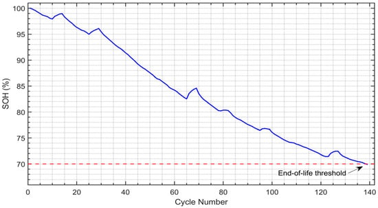
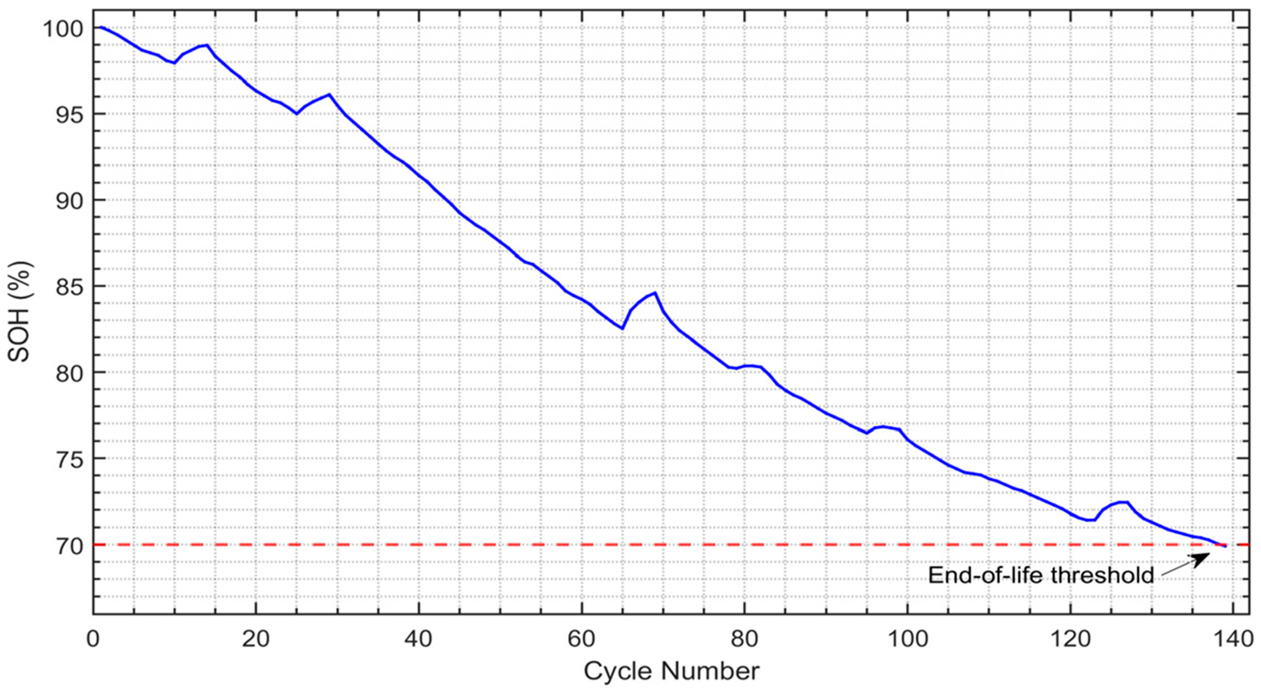
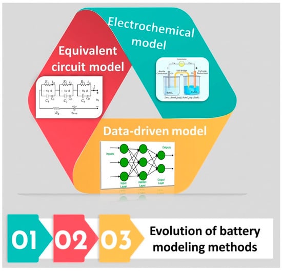
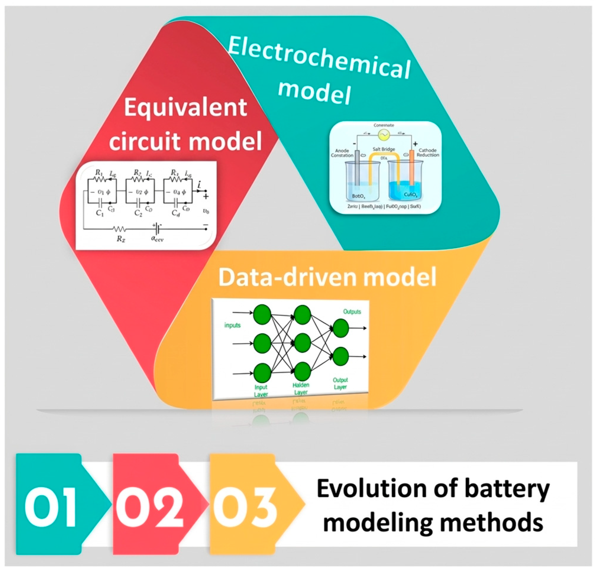
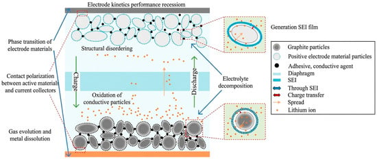
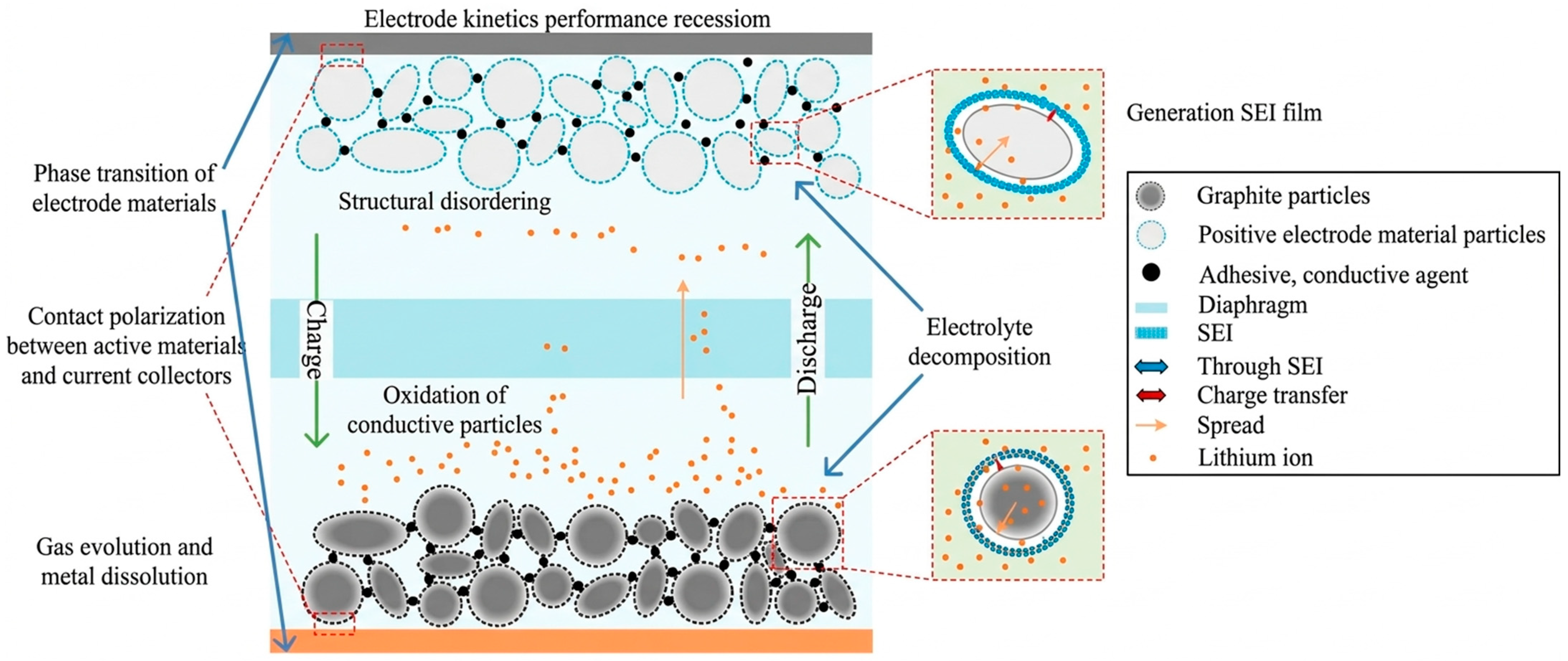
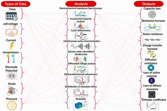
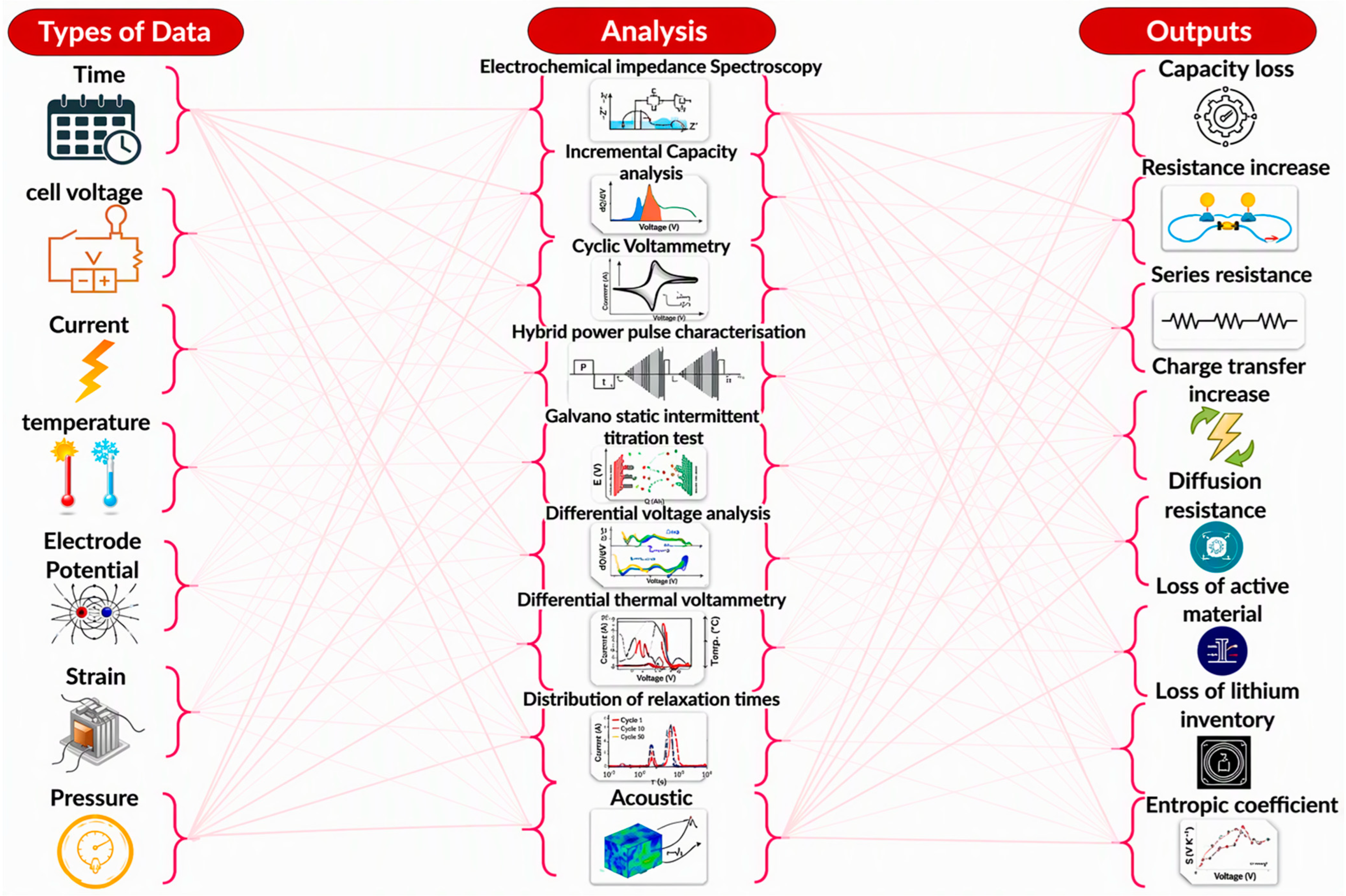
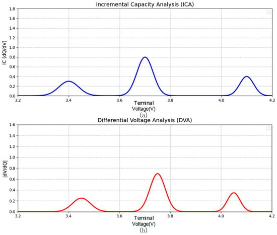
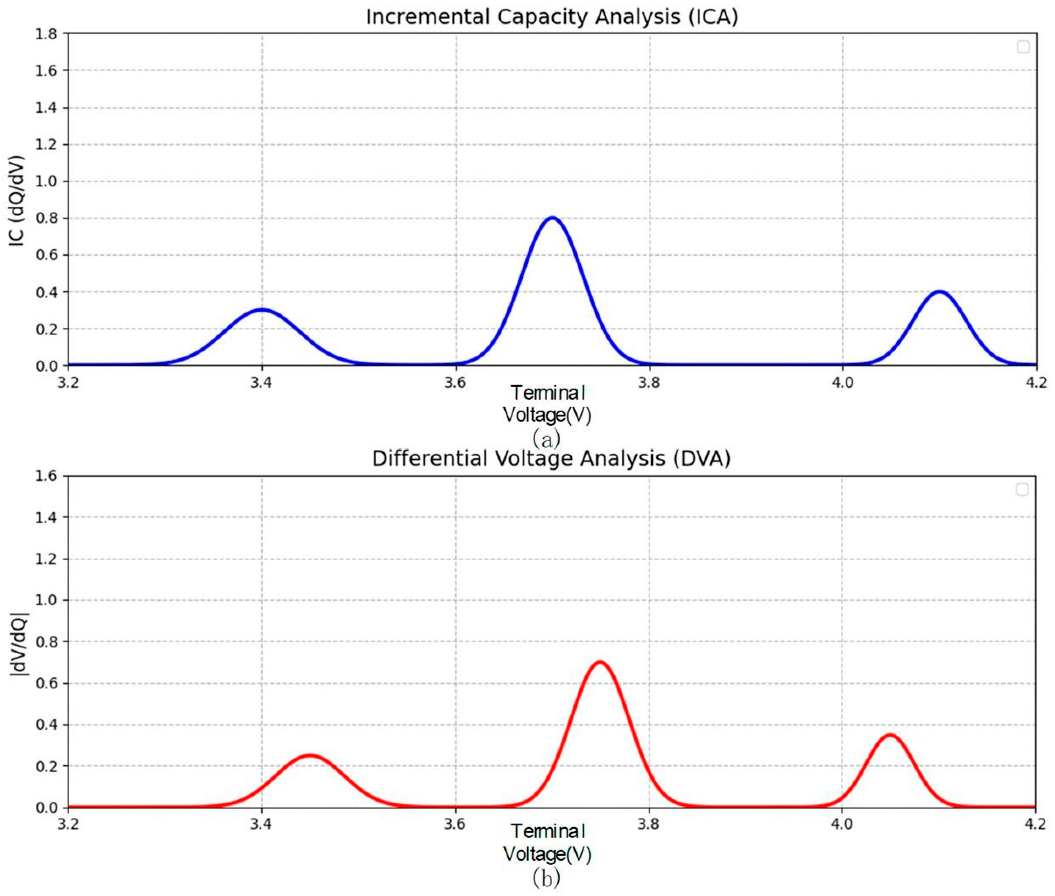
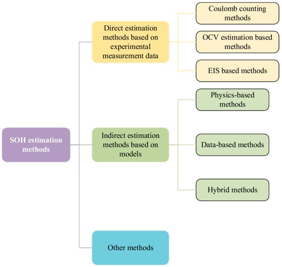
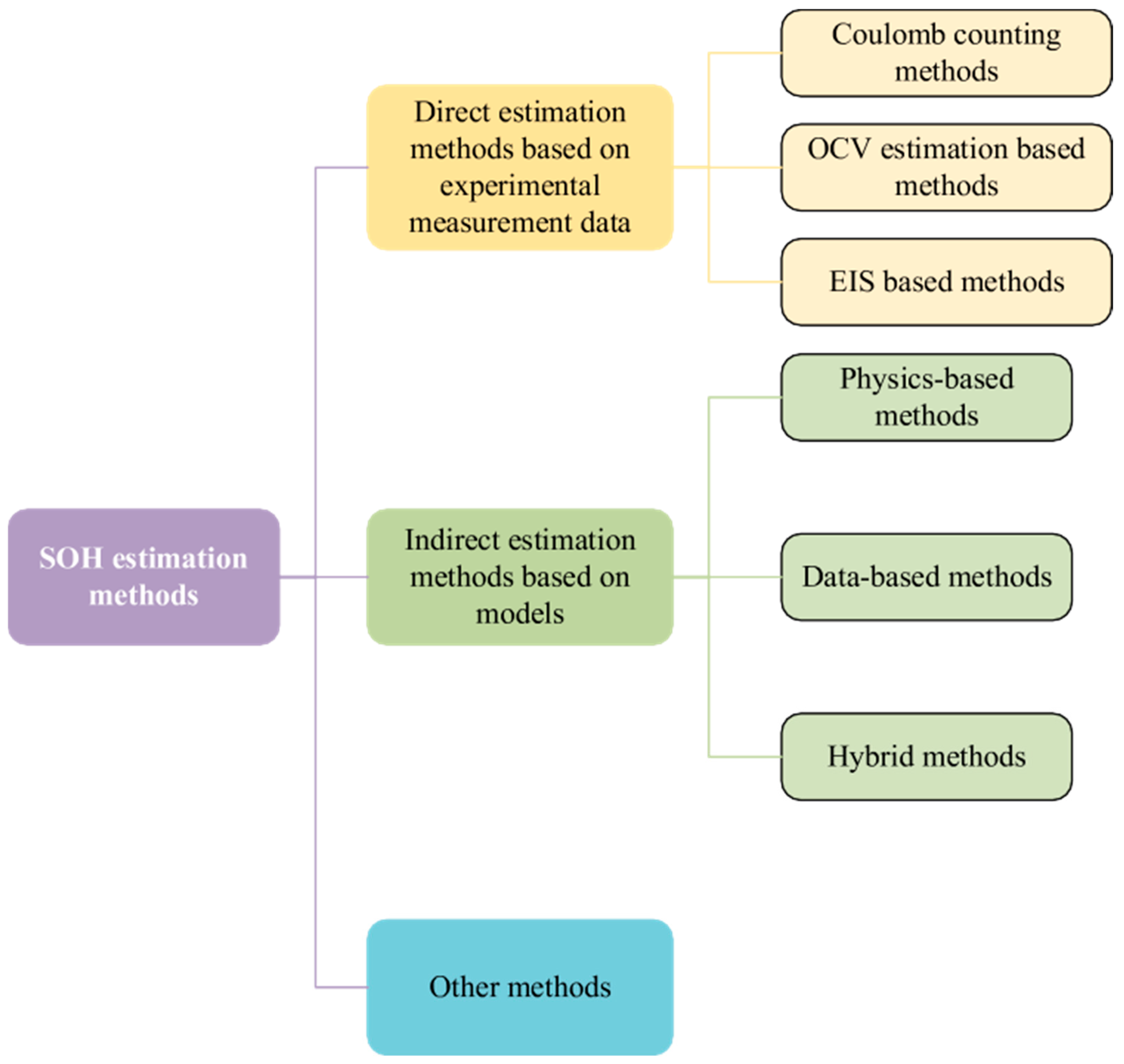
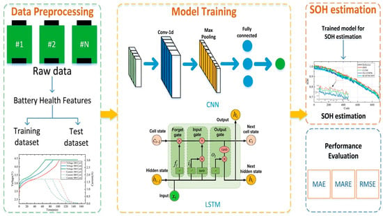
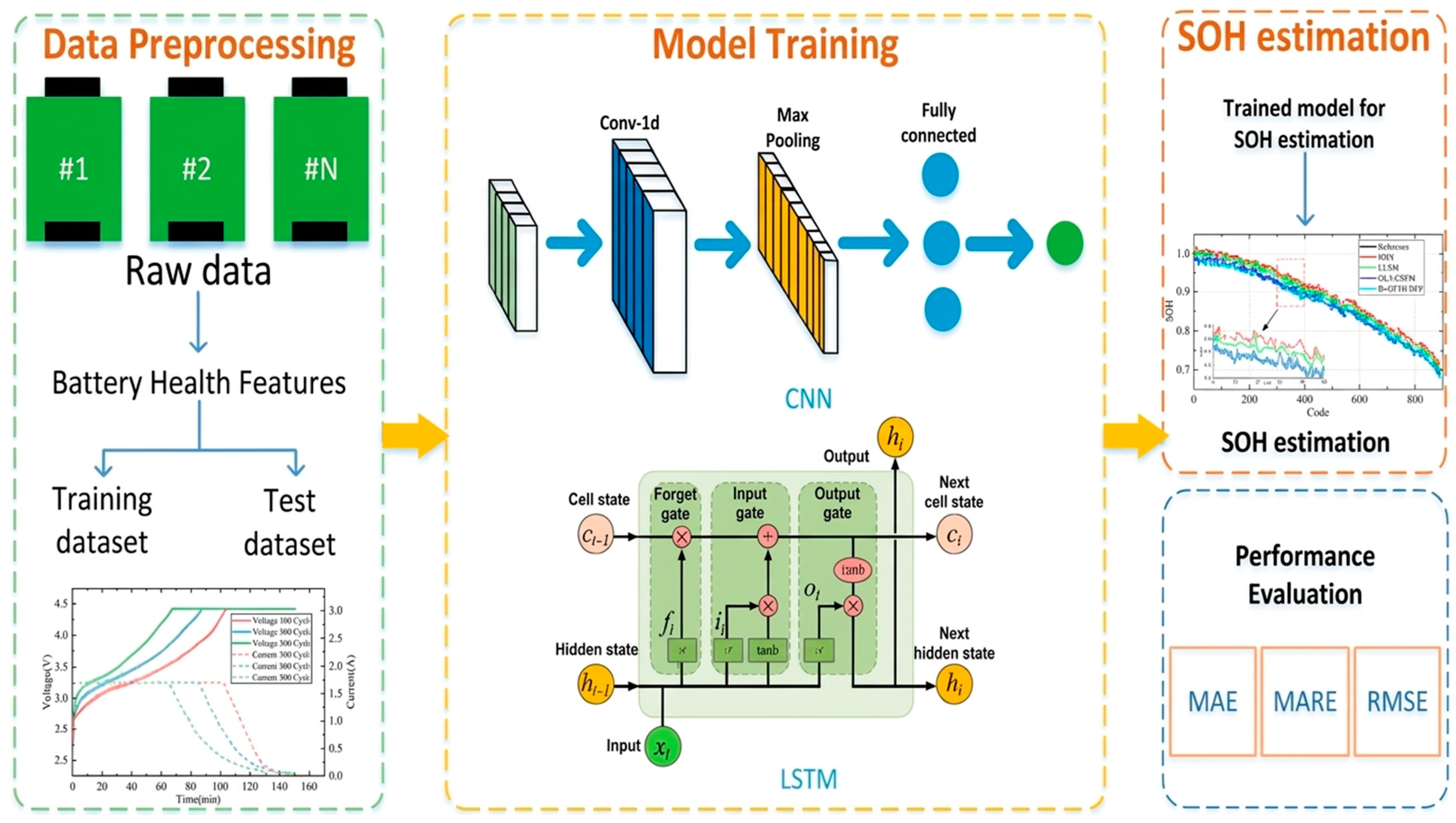
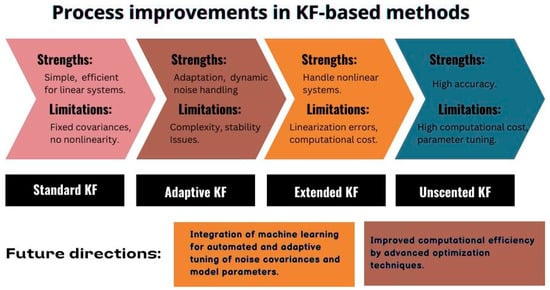
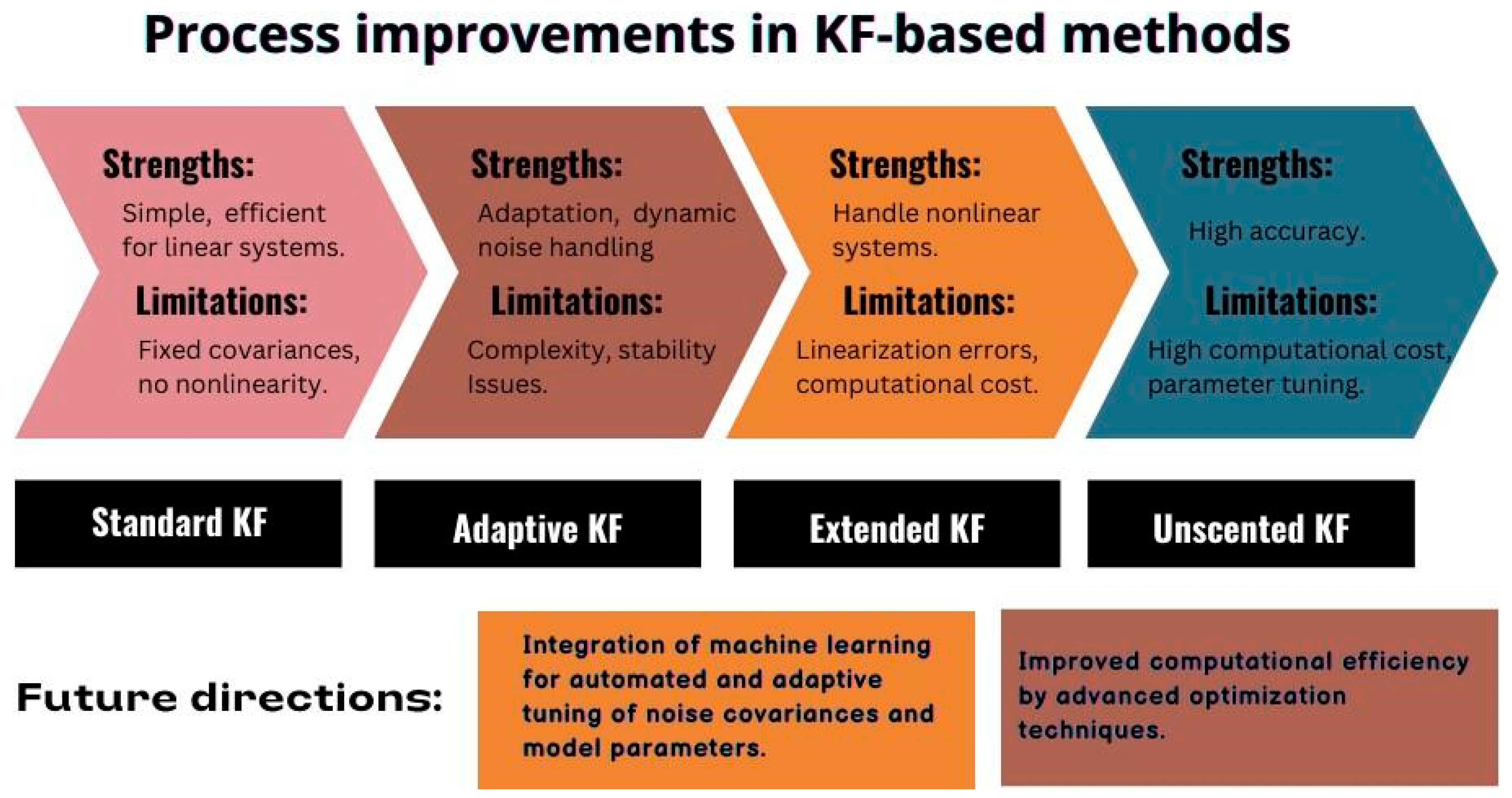
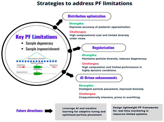
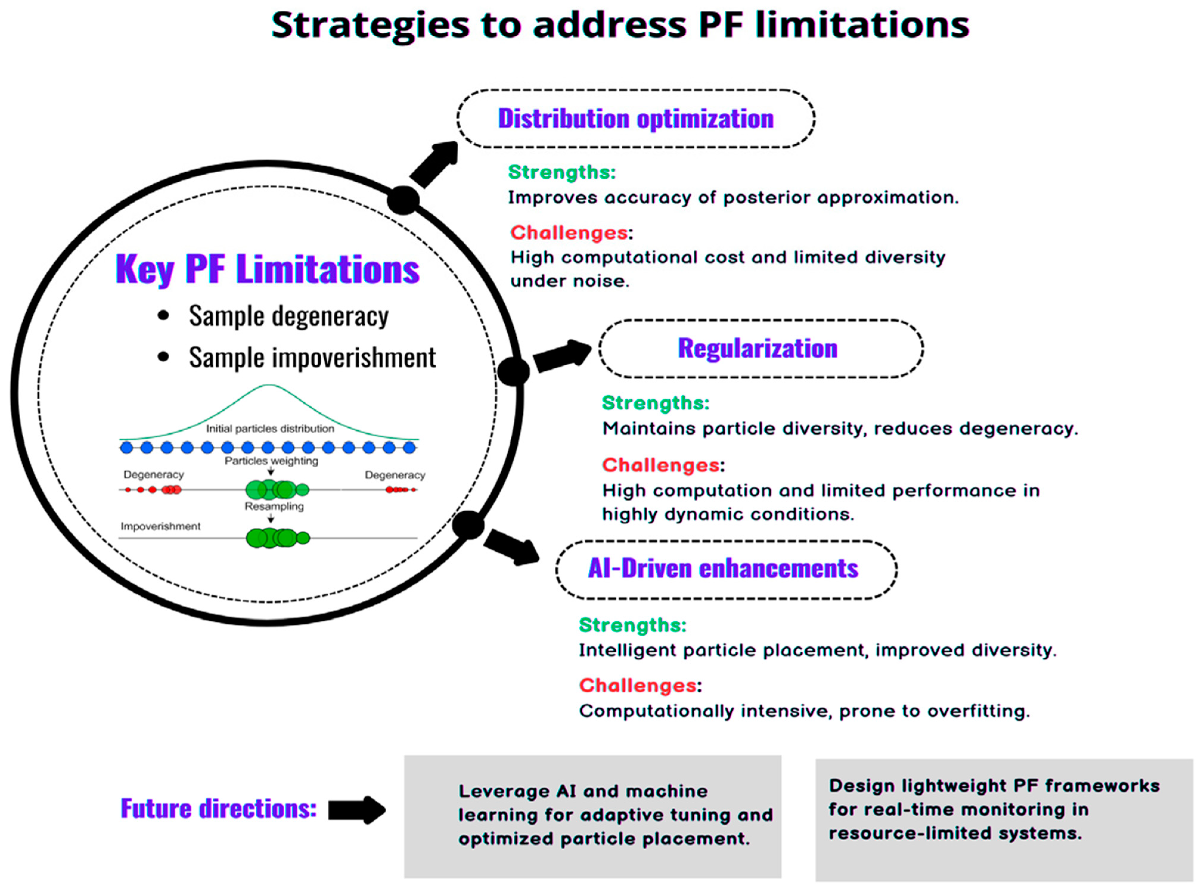
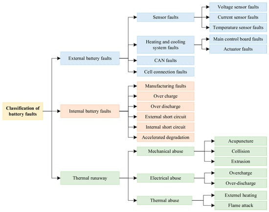
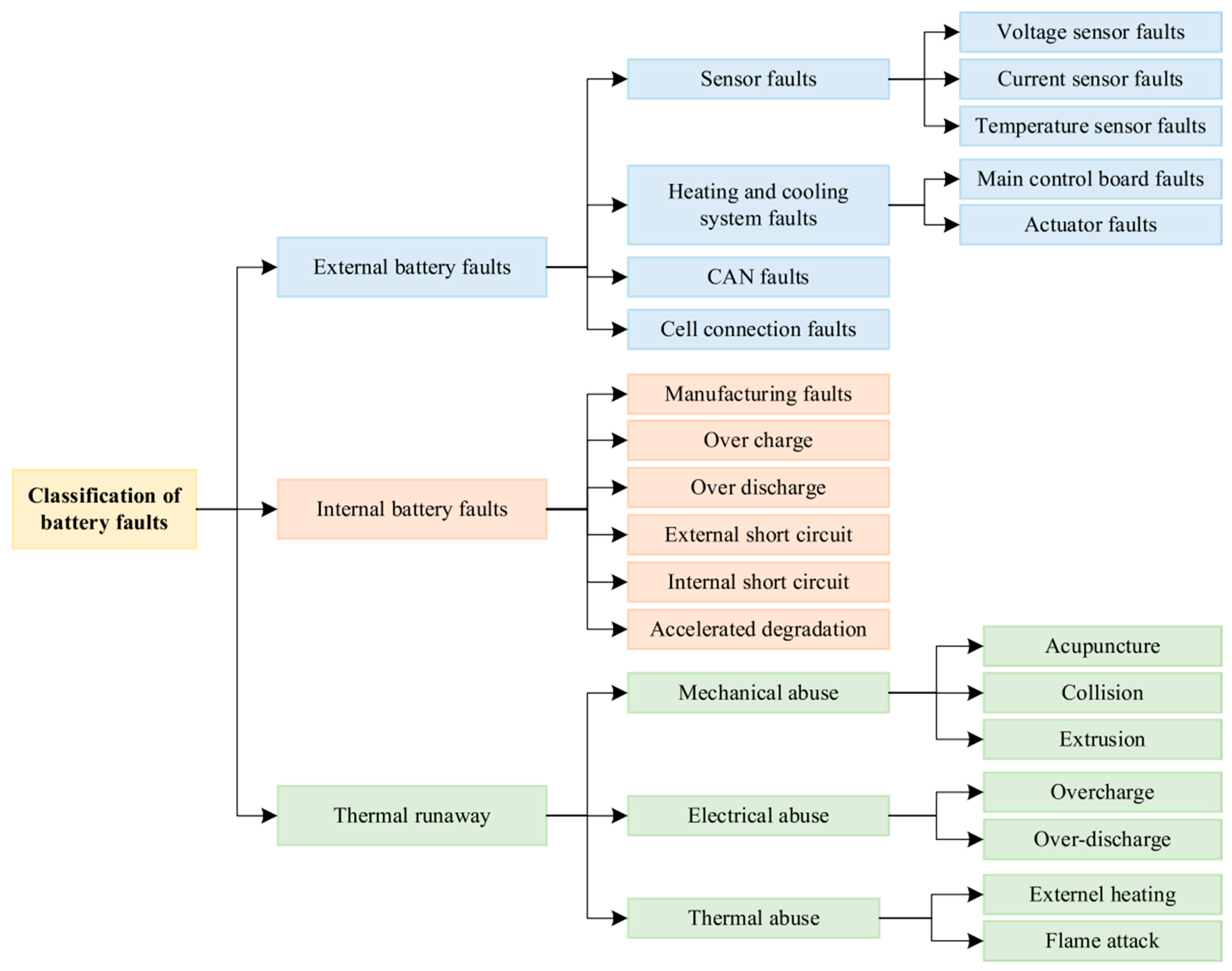
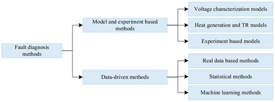
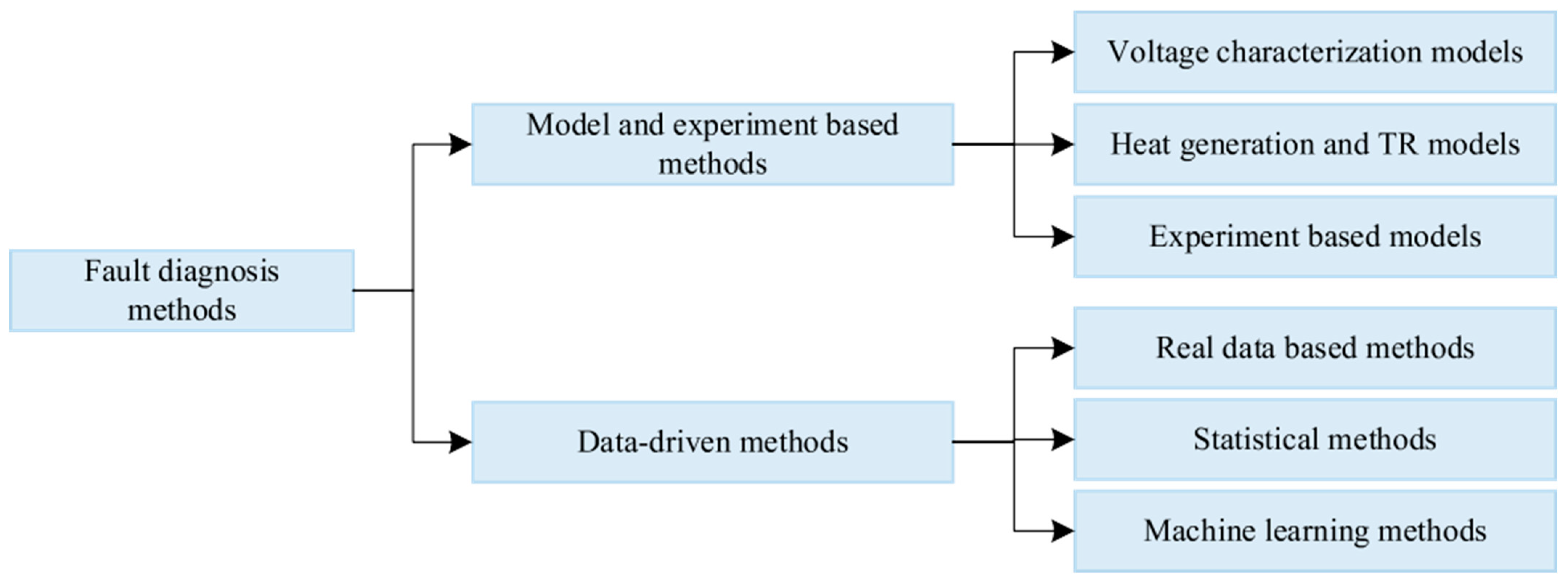
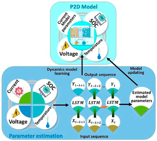
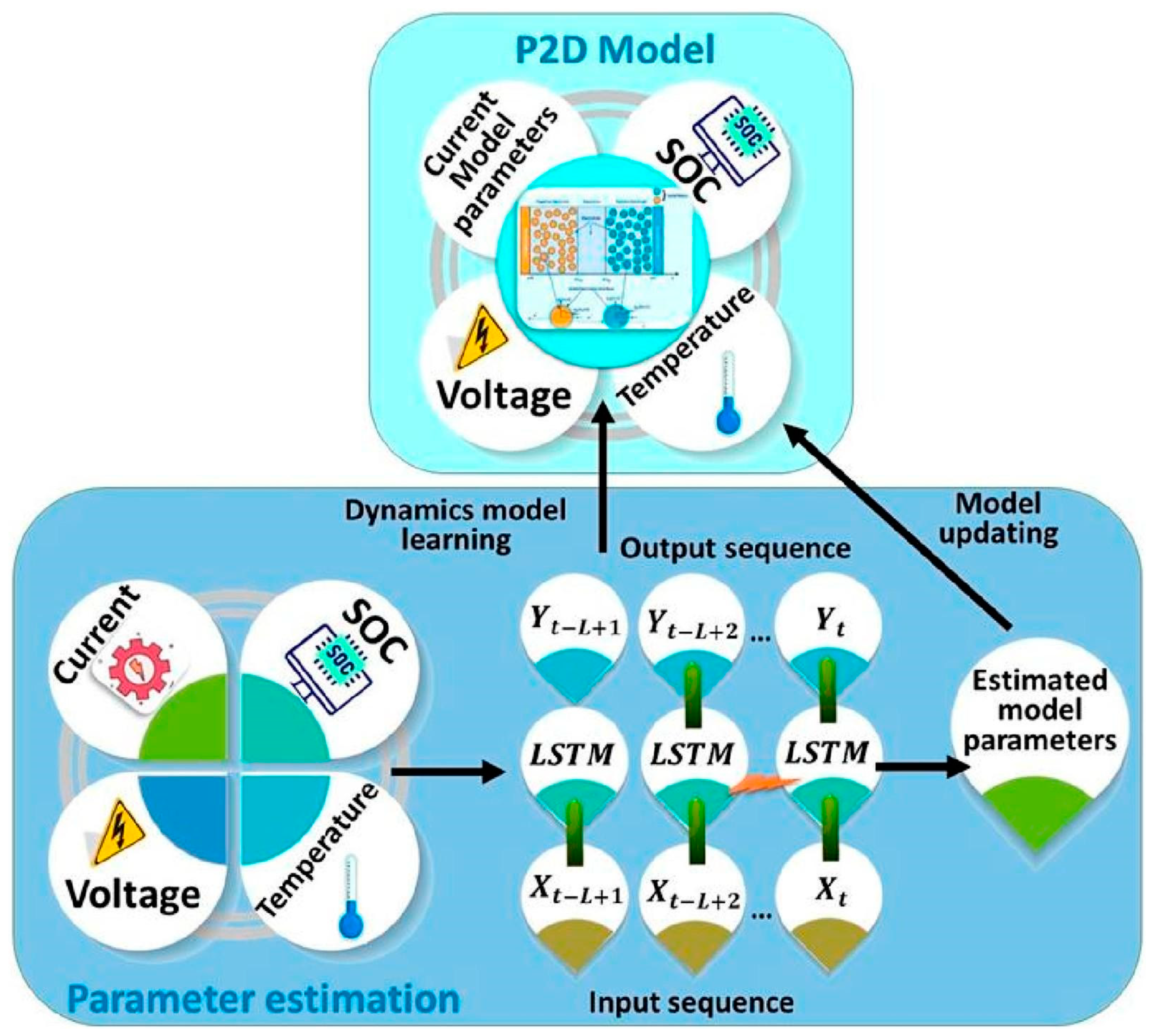
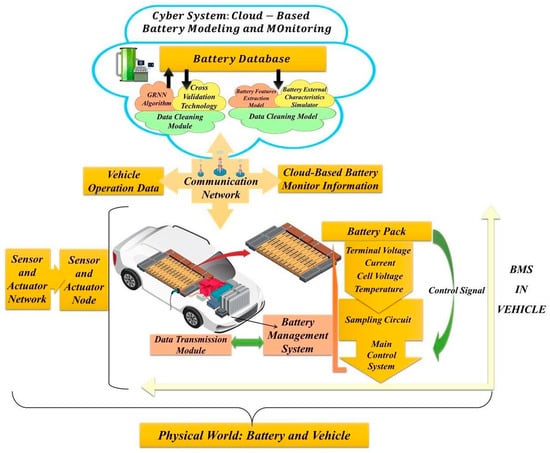
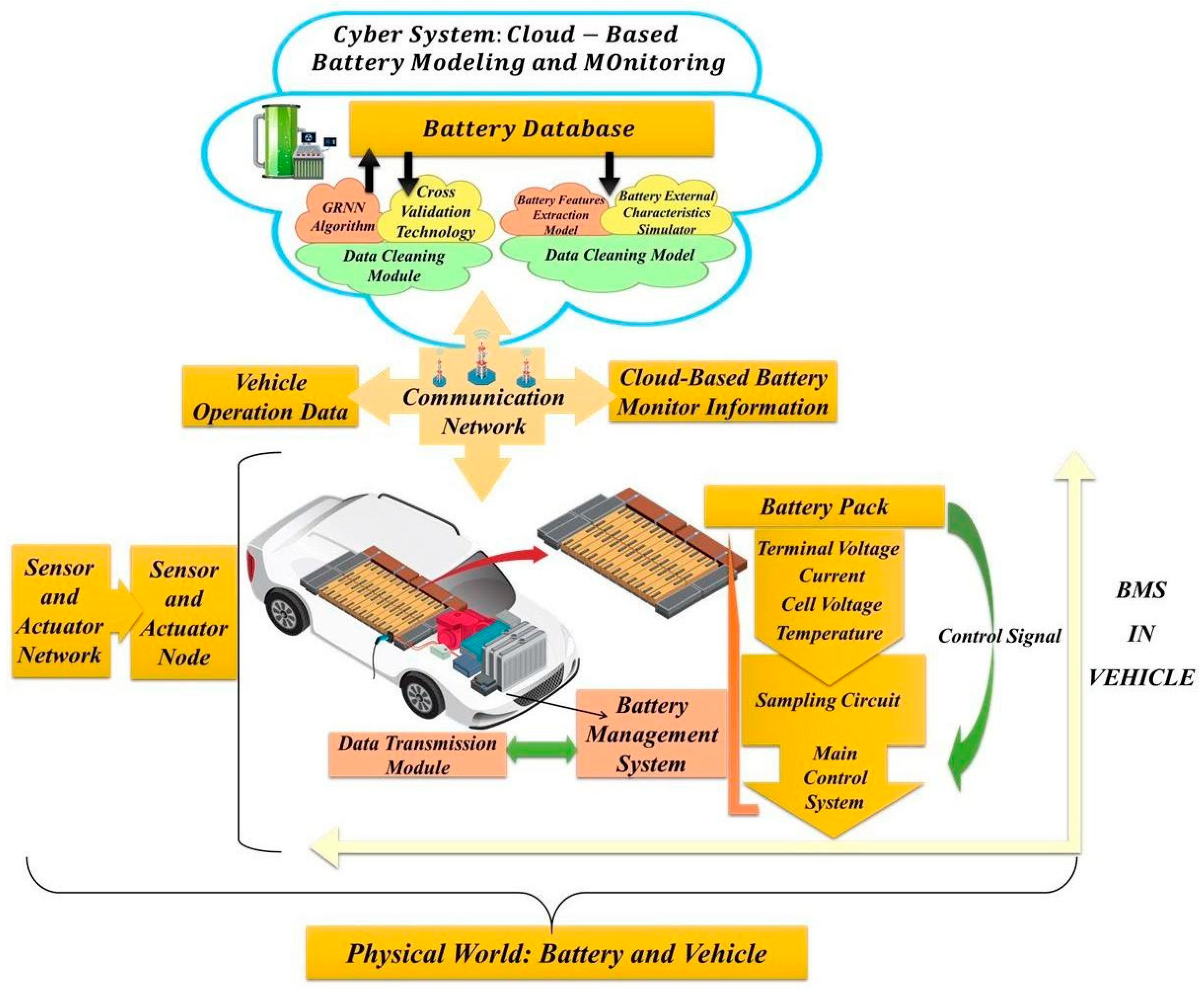
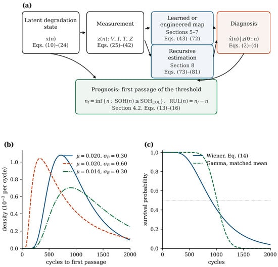
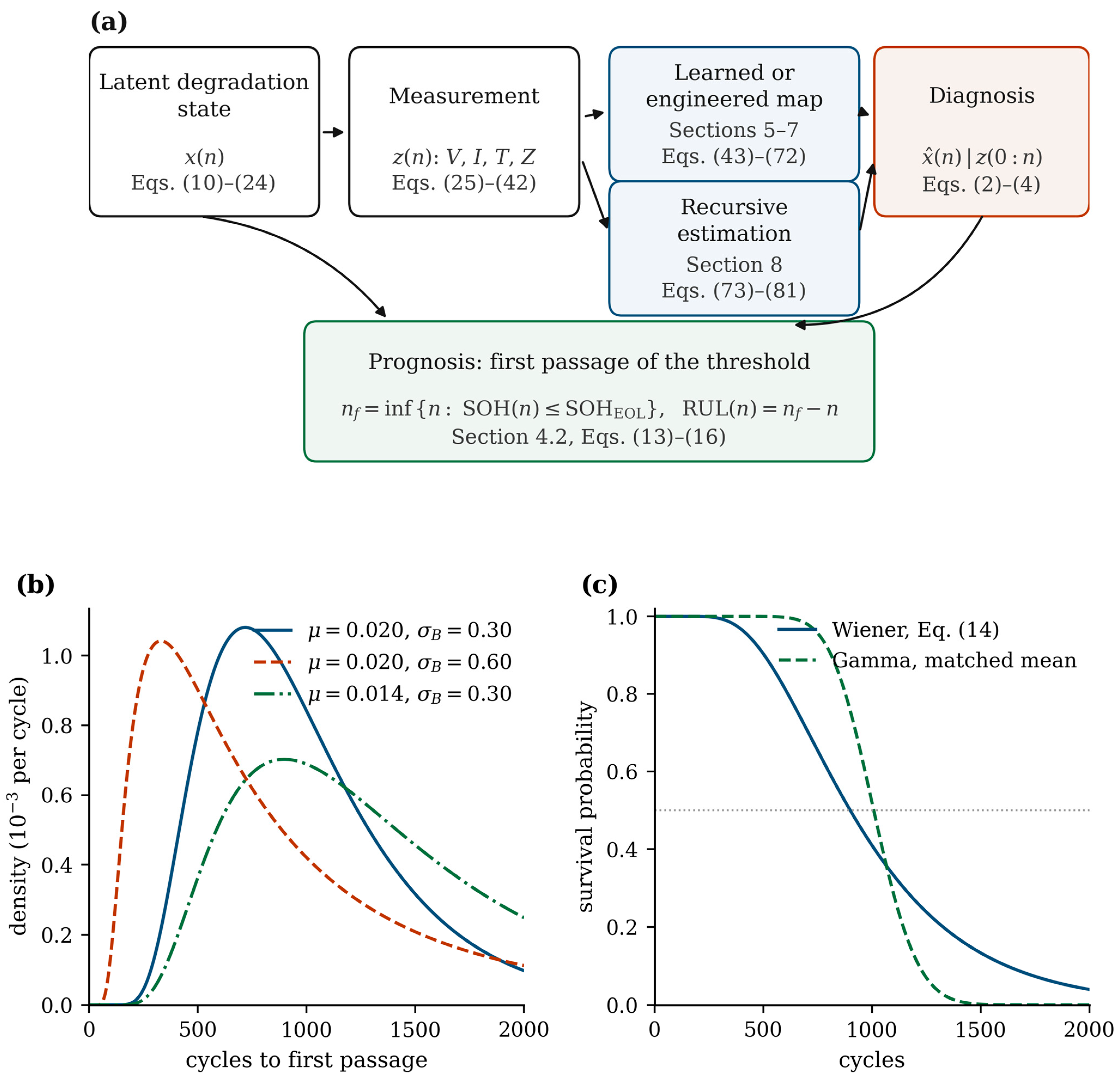

Disclaimer/Publisher’s Note: The statements, opinions and data contained in all publications are solely those of the individual author(s) and contributor(s) and not of MDPI and/or the editor(s). MDPI and/or the editor(s) disclaim responsibility for any injury to people or property resulting from any ideas, methods, instructions or products referred to in the content. |
© 2026 by the authors. Licensee MDPI, Basel, Switzerland. This article is an open access article distributed under the terms and conditions of the Creative Commons Attribution (CC BY) license.