Modeling Tumor–Immune Interactions Under Immuno-Chemotherapy: Stability Analysis and Numerical Simulation

Abstract

Advancements in tumor immunology and immunotherapy demonstrate that the immune system plays a crucial role in protecting the body against tumors and may be utilized to prevent or treat them. To investigate this further, we propose a mathematical model to study the complex dynamics of tumor–immune interactions under combined treatment: immunotherapy and chemotherapy. The proposed model consists of six coupled nonlinear ordinary differential equations (ODEs) describing the interaction of tumor cells with specific immune system components (immunostimulatory and immunosuppressive intermediates) and the effects of chemotherapy and immunotherapy. The antigen-presenting cells (APCs), specifically dendritic cells, are incorporated as the immunotherapy. We examine the essential characteristics of the system’s solutions, including existence, boundedness, and positivity. Furthermore, we investigate the presence and stability of equilibrium in two scenarios: intervention of immunotherapy alone and combined use of chemotherapy and immunotherapy. Each model exhibits two equilibria: a tumor-free equilibrium and a tumorous equilibrium. The stability analysis outlines the dynamic behavior associated with each equilibrium point. Additionally, we performed a sensitivity analysis and numerical simulations to validate our theoretical findings empirically. Using numerical simulations and stability analysis, we investigated the effects of treatments on tumor–immune dynamics.

1. Introduction

The immune system comprises a complex network of cells, tissues, and organs that preserve the integrity of the body by recognizing and eliminating harmful pathogens (such as bacteria, viruses, and parasites) and abnormal cells, including malignant tumor cells [1]. The lymphocytes (including T cells, B cells, and Natural Killer (NK) cells), monocytes/macrophages, and neutrophils are the predominant cells of the immune system, which help to identify specific antigens on malignant cells [2]. These lymphocytes can detect and initiate targeted invasions to eliminate tumor cells, hence restricting tumor proliferation [3]. Thus, lymphocyte concentrations indicate the immune response of an individual against the tumor [4]. This process is known as tumor immunosurveillance. However, tumors often evade immune surveillance through immune escape mechanisms, resulting in an immunosuppressive tumor microenvironment that promotes the growth of tumor cells [5]. Myeloid-derived suppressor cells (MDSCs) play a crucial role in this evasion, significantly contributing to immunosuppression, metastatic progression, and resistance to drug therapy [6]. Due to the complex relationship between tumors and immune cells, it is essential to understand tumor–immune system dynamics before developing effective immunotherapies [7].

Tumor immunotherapy is a treatment that utilizes the immune system’s innate ability to recognize and kill tumor cells, thereby counteracting tumor immune evasion and immunosuppression. It enhances the host’s immune response by utilizing external immunomodulatory substances, thereby improving its natural ability to identify and destroy tumor cells [8]. Dendritic cells (DCs) are specialized antigen-presenting cells (APCs) that play a crucial role in initiating and regulating immune responses. They connect the innate and adaptive immune systems to enhance immune surveillance [9]. In recent decades, dendritic cells (DCs) have been extensively studied as a foundation for tumor vaccines. Clinical studies indicate that immunotherapies based on dendritic cells produce higher response rates and enhance tumor eradication compared to other types of vaccines [10]. Therefore, we have incorporated dendritic cells as an immunotherapeutic element in this study, thereby boosting the immune response and enhancing tumor eradication outcomes.

Despite advances in the development of immunotherapy for tumors, considerable effort remains to establish immunotherapy as the standard of care for immune-sensitive tumors and to expand its applicability to a broader range of tumors [11]. Thus, the combination of immunotherapy and chemotherapy has emerged as a practical approach in modern oncology. Multiple studies and experimental investigations have shown that the simultaneous application of immunotherapy and chemotherapy yields favorable therapeutic results, often exhibiting greater efficacy [12,13]. Although the medical sector has conducted extensive studies on the relationship between tumors and the immune system, mathematical modeling offers a valuable complementary approach. This method is effective for predicting and analyzing tumor–immune–drug interactions. It helps forecast treatment outcomes and responses to medication in a cost-effective and time-efficient way. Additionally, mathematical modeling allows for a systematic analysis of immune dynamics and tumor behavior, providing insights that are often not attainable through experimental methods alone [14,15,16]. The current literature offers an extensive array of mathematical models that thoroughly examine various facets of tumor–immune system interactions [17,18,19,20]. These mathematical models support significant analyses, including the optimization of treatment strategies [21], stability and bifurcation analysis [22], and parameter estimation [23,24]. Additionally, numerical simulations are crucial in validating model predictions and exploring the system dynamics under different biological conditions [25].

In this study, we extended the tumor–immune model by Tran et al. [26] by incorporating the effects of immunotherapy through the administration of dendritic cells as an immunotherapeutic intervention. We also investigate the system’s dynamic behavior and conduct a comprehensive quantitative analysis of the extended model.

The paper framework is as follows: Section 1 contributes to the understanding and development of the tumor–immune model. Following that, Section 2 presents the mathematical analysis of the model. Within this section, Section 2.1 discusses the boundedness and positivity of the solutions of the model, while Section 2.2 and Section 2.3 explore the dynamics, including the existence of equilibrium points and their stability analysis, both in the context of immunotherapy alone and the context of immuno-chemotherapy, respectively. In Section 3, sensitivity analysis is performed. Eventually, Section 4 provides a comprehensive numerical simulation, while Section 5 summarizes our conclusions.

Mathematical Model

This section establishes a mathematical model to outline the interactions between tumor–immune system. The mathematical model presents a systematic strategy for describing the complex biological system, enabling an understanding of its fundamental mechanisms and dynamics. The model is expanded from the original model of Tran et al. [26] by adding a dendritic cell (D) interaction (fourth equation of model (1)) to describe immunotherapy and investigate the combined effects of chemotherapy and immunotherapy. Besides, Tran et al. [26] considered exponential growth for tumor cells and did not include saturation or crowding terms to describe tumor growth, as the available experimental data derived from in vivo mouse studies, where tumors are never allowed to reach their maximum size due to ethical constraints. However, in various models, tumor growth is modeled as Bertalanffy growth [27], logistic growth [28], power growth [29], and Gompertzian growth [30]. The logistic and Gompertzian growth models are among the most well-known and widely used because they accurately describe biological growth processes [31,32]. Therefore, in this study, we consider tumor growth to follow a logistic growth model.

The model comprises a system of six coupled ODEs, namely chemotherapy drug $\left(X\right)$, tumor cells $\left(T\right)$, immune cells $\left(I\right)$, dendritic cells $\left(D\right)$, immunostimulating mediators $\left(Y\right)$, and immunosuppressive intermediates $\left(Z\right)$. The following ODEs describe the proposed mathematical model for tumor–immune interplay:

$$\begin{array}{cc}\hfill {\displaystyle \frac{dX}{dt}}& =u-{\displaystyle \frac{k_{1}X}{k_2+X}},\hfill \\ \hfill {\displaystyle \frac{dT}{dt}}& =k_a\left(1-TK\right)T-{\displaystyle \frac{k_{b}XT}{k_c+T}}-k_{d}TI,\hfill \\ \hfill {\displaystyle \frac{dI}{dt}}& =Y-k_{e}TI-k_{f}XI-k_{g}ZI-k_{h}I+{\displaystyle \frac{{\alpha }_{1}D}{g_1+I}},\hfill \\ \hfill {\displaystyle \frac{dD}{dt}}& =s_d+{\displaystyle \frac{{\alpha }_{2}T}{g_2+T}}-{\delta }_{d}D,\hfill \\ \hfill {\displaystyle \frac{dY}{dt}}& ={\displaystyle \frac{X}{1+X/k_i}}-k_{j}Y-k_{k}YZ,\hfill \\ \hfill {\displaystyle \frac{dZ}{dt}}& ={\displaystyle \frac{I}{1+X/k_l}}-k_{m}XZ-{\delta }_{Z}Z,\hfill \end{array}$$

(1)

• The first equation of (1) represents the drug concentration at time t that is cleared at saturated rate ${\displaystyle \frac{k_{1}X}{k_2+X}}$. The constant source rate of the drug is denoted as u.
• The second equation of (1) describes the density of tumor cells at any time t. Term $k_a\left(1-TK\right)T$ describes the logistic growth of tumor cells without any immune response. Tumor cells are killed due to interaction with the drug $X\left(t\right)$ at a rate $k_b$, and by immune cells $I\left(t\right)$ at a rate $k_d$. The ratio ${\displaystyle \frac{k_{b}T}{k_c+T}}$ is the cytotoxic death term.
• The dynamics of immune cells are explained in the third equation of (1). The immunostimulating mediators $Y\left(t\right)$ activate immune cells. The exhaustion rate is $k_e$, whereas $k_f$ is the death rate of immune cells due to the tumor, and $k_g$ is the immunosuppression rate. The natural decay rate of immune cells is $k_h$. However, ${\alpha }_1$ is the growth rate of immune cells boosted by dendritic cells $D\left(t\right)$.
• The density of antigen-presenting dendritic cells is described in the fourth equation of (1). The constant source rate of dendritic cells is $s_d$, whereas ${\alpha }_2$ is the activation rate due to the direct presence of tumor cells, and $g_2$ is the half-saturation constant. The natural death rate of dendritic cells is ${\delta }_d$.
• The concentration of immunostimulating mediators $Y\left(t\right)$ is stated in the fifth equation of (1), which is increased by drug $X\left(t\right)$ according to saturating function ${\displaystyle \frac{X}{1+X/k_i}}$. It is assumed to decay at a rate of $k_j$ and is inactivated due to interactions with immune-suppressive mediator $Z\left(t\right)$ at $k_k$ rate.
• The last equation of (1) represents the immune-suppressive mediator $Z\left(t\right)$, activated by $I\left(t\right)$. Its effectiveness is influenced by $X\left(t\right)$ accordingly as ${\displaystyle \frac{I}{1+X/k_l}}$. Additionally, $Z\left(t\right)$ decays at a rate of ${\delta }_Z$, and is further reduced at a rate of $k_m$ through its interaction with the drug $X\left(t\right)$.

Table 1 provides thorough descriptions of all model parameters. All the parameters are considered to be positive. Using the following weights, we non-dimensionalized model (1) for convenience.

Table 1. Specification of variables and constants of the model (1).

Variables	Specification
X	therapeutic concentration (chemotherapy drug)
T	tumor cells density
I	immune cells density
D	dendritic cells concentration
Y	immunostimulating mediators
Z	immune-suppressor mediators
u	constant therapeutic source rate
$k_1$	maximum therapeutic metabolic rate
$k_2$	half-maximal metabolic concentration
$K^{-1}$	saturation of tumor growth
$k_a$	tumor proliferation rate
$k_b$	drug-induced tumor cell death rate
$k_c$	half-maximal effective concentration
$k_d$	immune-mediated tumor cell decay constant
$k_e$	tumor-induced immune cell decay constant
$k_f$	drug-induced immune cell death constant
$k_g$	immune-suppressive mediator–induced immune cell death constant
$k_h$	natural decay of immune cells
${\alpha }_1$	activation rate of immune cells due to dendritic cells
$g_1$	half saturation constant of immune cell for half-maximal dendritic cells
$s_d$	constant source rate of dendritic cells
${\alpha }_2$	activation rate of dendritic cells due to tumor cells
$g_2$	tumor cell level for half-maximal dendritic cells
${\delta }_d$	natural death rate of dendritic cells
$k_i$	half-maximal effective concentration of immunostimulating mediators
$k_j$	natural decay of immunostimulating mediators
$k_k$	decay rate of immunostimulating mediators due to immune-suppressive mediator
$k_l$	half-maximal effective concentration of immune-suppressive mediators
$k_m$	drug-mediated degradation rate of immune-suppressor mediators
${\delta }_Z$	natural death rate of immune-suppressor mediators

$X=\overline{X},T={\displaystyle \frac{\overline{T}}{K}},I={\displaystyle \frac{k_a}{k_d}}\overline{I},D={\displaystyle \frac{s_d}{k_a}}\overline{D},Y={\displaystyle \frac{k_a^2}{k_d}}\overline{Y},Z={\displaystyle \frac{k_a}{k_g}}\overline{Z},t={\displaystyle \frac{1}{k_a}}\overline{t}$.

Further, dropping the over-line for notional clarity (that is, by letting $\overline{t}=t$, $\overline{T}=T$, $\overline{I}=I$, $\overline{D}=D$, $\overline{X}=X$, $\overline{Y}=Y$, and $\overline{Z}=Z$.), the non-dimensionalized model is as follows:

$$\begin{array}{cc}\hfill {\displaystyle \frac{dX}{dt}}& =a_1-{\displaystyle \frac{a_{2}X}{a_3+X}},\hfill \\ \hfill {\displaystyle \frac{dT}{dt}}& =(1-T)T-{\displaystyle \frac{a_{4}XT}{a_5+T}}-TI,\hfill \\ \hfill {\displaystyle \frac{dI}{dt}}& =Y-a_{6}TI-a_{7}XI-ZI-a_{8}I+{\displaystyle \frac{a_{9}D}{a_{10}+I}},\hfill \\ \hfill {\displaystyle \frac{dD}{dt}}& =1+{\displaystyle \frac{a_{11}T}{a_{12}+T}}-a_{13}D,\hfill \\ \hfill {\displaystyle \frac{dY}{dt}}& ={\displaystyle \frac{a_{14}X}{a_{15}+X}}-a_{16}Y-a_{17}YZ,\hfill \\ \hfill {\displaystyle \frac{dZ}{dt}}& ={\displaystyle \frac{a_{18}I}{a_{19}+X}}-a_{20}XZ-a_{21}Z,\hfill \end{array}$$

(2)

where $a_1={\displaystyle \frac{u}{k_a}}$, $a_2={\displaystyle \frac{k_1}{k_a}}$, $a_3=k_2$, $a_4={\displaystyle \frac{k_{b}K}{k_a}}$, $a_5=k_{c}K$, $a_6={\displaystyle \frac{k_e}{K{k}_a}}$, $a_7={\displaystyle \frac{k_f}{k_a}}$, $a_8={\displaystyle \frac{k_h}{k_a}}$, $a_9={\displaystyle \frac{{\alpha }_1{s}_d{k}_d^2}{k_a^4}}$, $a_{10}={\displaystyle \frac{g_1{k}_d}{k_a}}$, $a_{11}={\displaystyle \frac{{\alpha }_2}{s_d}}$, $a_{12}=g_{2}K$, $a_{13}={\displaystyle \frac{{\delta }_d}{k_a}}$, $a_{14}={\displaystyle \frac{k_d{k}_i}{k_a^3}}$, $a_{15}=k_i$, $a_{16}={\displaystyle \frac{k_j}{k_a}}$, $a_{17}={\displaystyle \frac{k_k}{k_g}}$, $a_{18}={\displaystyle \frac{k_l{k}_g}{k_a{k}_d}}$, $a_{19}=k_l$, $a_{20}={\displaystyle \frac{k_m}{k_a}}$, $a_{21}={\displaystyle \frac{{\delta }_Z}{k_a}}$. All constants $a_1,a_2,\dots ,a_{21}$ are positive.

2. Theoretical Analysis of the Model

This section focuses on establishing the positivity and boundedness of the solutions of the system (2). After that, the existence and stability behavior of the steady-state solutions of system (2) are investigated in the absence as well as in the presence of chemotherapy.

2.1. Boundedness and Positivity

The boundedness of the solutions to the system (2) under positive initial conditions is examined in this section, ensuring the well-posedness of the model. The phase space of system (2) is given by $\Theta =\left\{(X,T,I,D,Y,Z)\in {\mathbb{R}}_{+}^6\right\}$. The following theorem ensures the positivity and boundedness of the solutions of system (2).

Theorem 1.

For all initial conditions within the set Θ, the solutions of system (2) remain confined to the domain Ψ, which is bounded provided $a_2>a_1$, such that

$$\Psi =\left\{(X,T,D,I,Y,Z)\in {\mathbb{R}}_{+}^6|0<X\le X_m,0<T\le T_m,0<I\le I_m,0<D\le D_m,0<Y\le Y_m,0<Z\le Z_m\right\},$$

where $X_m,T_m,D_m,Y_m,I_m$ and $Z_m$ are positive constants constructed in the proof (see (3)–(8) respectively).

Proof. 

Initially, we examine the positivity of $X\left(t\right)$. We assume $X\left(0\right)\ge 0$. Then, for $X\left(t\right)<0$ for some $t>0$, we should have ${\displaystyle \frac{dX}{dt}}\le 0$ when $X=0$. However, we have

$${{\displaystyle \frac{dX}{dt}}|}_{X=0}=a_1>0,$$

Thus, $X\left(t\right)>0\forall t\ge 0$.

For the positivity of $T\left(t\right)$, consider the second equation of (2),

$$\begin{array}{cc}\hfill {\displaystyle \frac{dT}{dt}}& =(1-T)T-{\displaystyle \frac{a_{4}XT}{a_5+T}}-TI,\hfill \\ \hfill & =f\left(t\right)T.\hfill \end{array}$$

Thus, we have

$$T\left(t\right)=T\left(0\right)e^{{\int }_0^{t}f\left(s\right)ds}$$

where $f\left(t\right)=1-T-{\displaystyle \frac{a_{4}X}{a_5+T}}-I$. We initially assumed $T\left(t\right)$ to be positive. Thus, $T\left(t\right)>0\forall t\ge 0$.

Subsequently, from the fourth equation of system (2), we have

$$\begin{array}{cc}\hfill {\displaystyle \frac{dD}{dt}}& =1+{\displaystyle \frac{a_{11}T}{a_{12}+T}}-a_{13}D,\hfill \\ \hfill & \ge -a_{13}D.\hfill \end{array}$$

Thus, $D\left(t\right)\ge C_2{e}^{-a_{13}}t,$ which indicates that $D\left(t\right)>0$ for all $t\ge 0$ as initially $D\left(t\right)$ is positive.

From the fifth equation of (2), we have

$${\displaystyle \frac{dY}{dt}}\ge (-a_{16}-a_{17}Z)Y.$$

Therefore, we obtain

$$Y\left(t\right)\ge C_3{e}^{(-a_{16}-a_{17}Z)t},$$

where $C_3$ is constant and initially $Y\left(t\right)$ is assumed positive. Hence, $Y\left(t\right)>0\forall t\ge 0$.

Now, for the positivity of $I\left(t\right)$, we know it is initially positive. Then, for $I\left(t\right)<0$ for some $t>0$, we should have ${\displaystyle \frac{dI}{dt}}\le 0$. However, from the third equation of (2), we obtain

$${{\displaystyle \frac{dI}{dt}}|}_{I=0}=Y+{\displaystyle \frac{a_{9}D}{a_{10}}}>0,$$

as we have already proved above, $D\left(t\right)$ and $Y\left(t\right)$ are positive. Thus, $I\left(t\right)>0\forall t\ge 0$.

Similarly, $Z\left(t\right)$ is also initialized positively. Thus, from the last equation of system (2), we have

$${{\displaystyle \frac{dZ}{dt}}|}_{Z=0}={\displaystyle \frac{a_{18}I}{a_{19}+X}}>0.$$

Hence, $Z\left(t\right)>0\forall t\ge 0$ as proved above that $I\left(t\right)>0\forall t\ge 0$ and $X\left(t\right)>0\forall t\ge 0$.

To ensure that the system solution (2) is bounded for all $t\ge 0$, we calculate the upper bound as follows:

For upper bound of $X\left(t\right)$, solve the first equation of (2). Then, we have

$$X\left(t\right)={\displaystyle \frac{-e^{-\frac{(a_2-a_1)((t+C_4)(a_2-a_1)+X)}{a_2{a}_3}}}{a_2-a_1}}+{\displaystyle \frac{a_3{a}_1}{a_2-a_1}},$$

where $C_4$ is constant. We have $\underset{t\to \infty }{lim}supX\left(t\right)\le {\displaystyle \frac{a_3{a}_1}{a_2-a_1}},\mathrm{if}{a}_2>a_1$. Thus, X is bounded above by

$$X_m=max\left(X\left(0\right),{\displaystyle \frac{a_3{a}_1}{a_2-a_1}}\right).$$

(3)

Considering the second equation of (2), we get ${\displaystyle \frac{dT}{dt}}\le (1-T)T.$ Then, $\underset{t\to \infty }{lim}supT\left(t\right)\le 1.$

Hence, T is bounded above by

$$T_m=max\left(T\left(0\right),1\right).$$

(4)

Now, for boundedness of $D\left(t\right)$, we have ${\displaystyle \frac{dD}{dt}}\le 1+{\displaystyle \frac{a_{11}{T}_m}{a_{12}}}-a_{13}D.$ Therefore, we get

$$D\left(t\right)\le {\displaystyle \frac{1}{a_{13}}}+{\displaystyle \frac{a_{11}{T}_m}{a_{12}{a}_{13}}}+C_5{e}^{-a_{13}t},$$

where $C_5$ is constant. Further, $\underset{t\to \infty }{lim}supD\left(t\right)\le {\displaystyle \frac{1}{a_{13}}}+{\displaystyle \frac{a_{11}{T}_m}{a_{12}{a}_{13}}}.$ Thus, $D\left(t\right)$ is bounded above by

$$D_m=max\left(D\left(0\right),{\displaystyle \frac{1}{a_{13}}}+{\displaystyle \frac{a_{11}{T}_m}{a_{12}{a}_{13}}}\right).$$

(5)

Considering fifth equation of (2), we have

$$\begin{array}{cc}\hfill {\displaystyle \frac{dY}{dt}}& \le {\displaystyle \frac{a_{14}{X}_m}{a_{15}}}-a_{16}Y.\hfill \end{array}$$

Thus, $Y\le {\displaystyle \frac{a_{14}{X}_m}{a_{15}{a}_{16}}}+C_6{e}^{-a_{16}t}$, where $C_6$ is constant. Taking, $\underset{t\to \infty }{lim}supY\left(t\right)\le {\displaystyle \frac{a_{14}{X}_m}{a_{15}{a}_{16}}}.$ Hence, Y is bounded above by

$$Y_m=max\left(Y\left(0\right),{\displaystyle \frac{a_{14}{X}_m}{a_{15}{a}_{16}}}\right).$$

(6)

Now, from the third equation of (2), ${\displaystyle \frac{dI}{dt}}\le Y_m+{\displaystyle \frac{a_9{D}_m}{a_{10}}}-a_{8}I.$

Hence, we have

$$I\left(t\right)\le {\displaystyle \frac{Y_m{a}_{10}+a_9{D}_m}{a_8{a}_{10}}}+C_7{e}^{-a_{8}t},$$

where $C_7$ is constant. Let us consider, $\underset{t\to \infty }{lim}supI\left(t\right)\le {\displaystyle \frac{Y_m{a}_{10}+a_9{D}_m}{a_8{a}_{10}}}.$ Thus, I is bounded above by

$$I_m=max\left(I\left(0\right),{\displaystyle \frac{Y_m{a}_{10}+a_9{D}_m}{a_8{a}_{10}}}\right).$$

(7)

Further, from the last equation of system (2), we have

$$\begin{array}{cc}\hfill {\displaystyle \frac{dZ}{dt}}& \le {\displaystyle \frac{a_{18}{I}_m}{a_{19}}}-a_{21}Z.\hfill \end{array}$$

Hence, $Z\left(t\right)\le {\displaystyle \frac{a_{18}{I}_m}{a_{19}{a}_{21}}}-C_8{e}^{-a_{21}t},$ where $C_8$ is constant. Then, further $\underset{t\to \infty }{lim}supZ\left(t\right)\le {\displaystyle \frac{a_{18}{I}_m}{a_{19}{a}_{21}}}.$ Thus, the upper bound of Z is

$$Z_m=max\left(Z\left(0\right),{\displaystyle \frac{a_{18}{I}_m}{a_{19}{a}_{21}}}\right).$$

(8)

Therefore, the trajectories of solutions that originate positively from $\Theta$ are bounded in $\Psi$. □

2.2. Model Dynamics Under the Effect of Immunotherapy Alone

Within this section, we study the tumor–immune interaction model (2) in the absence of chemotherapy (i.e., $X=0$). Accordingly, we have a reduced model (9) that includes immune cells I, tumor cells T, dendritic cells D, and both immunostimulating mediators Y and immune-suppressive mediators Z. Thus, the transformed model is:

$$\begin{array}{cc}\hfill {\displaystyle \frac{dT}{dt}}& =(1-T)T-TI,\hfill \\ \hfill {\displaystyle \frac{dI}{dt}}& =Y-a_{6}TI-ZI-a_{8}I+{\displaystyle \frac{a_{9}D}{a_{10}+I}},\hfill \\ \hfill {\displaystyle \frac{dD}{dt}}& =1+{\displaystyle \frac{a_{11}T}{a_{12}+T}}-a_{13}D,\hfill \\ \hfill {\displaystyle \frac{dY}{dt}}& =-a_{16}Y-a_{17}YZ,\hfill \\ \hfill {\displaystyle \frac{dZ}{dt}}& ={\displaystyle \frac{a_{18}I}{a_{19}}}-a_{21}Z,\hfill \end{array}$$

(9)

where $a_6$, $a_8$, $a_9$, $a_{10}$, $a_{11}$, $a_{12}$, $a_{13}$, $a_{16}$, $a_{17}$, $a_{18}$, $a_{19}$, and $a_{21}$ are positive constants (as defined in (2)). Firstly, we will examine the steady state solutions of the system (9). Therefore, from the first equation of the reduced system (9), we have either $T=0$ or $T=1-I$. Thus, we have two types of equilibrium: tumorous (i.e., $T\ne 0$) and without tumor (i.e., $T=0$).

• Analysis of the tumor-free equilibrium and its stability: When $T=0$, the remaining equations of system (9) simplify to

  $$\left\{\begin{array}{c}-a_{18}{a}_{13}{I}^3+(-a_8{a}_{19}{a}_{21}{a}_{13}-a_{18}{a}_{13}{a}_{10})I^2-a_8{a}_{19}{a}_{21}{a}_{13}{a}_{10}I+a_9{a}_{19}{a}_{21}=0,\hfill \\ D={\displaystyle \frac{1}{a_{13}}},Y=0,\hfill \\ Z={\displaystyle \frac{a_{18}I}{a_{19}{a}_{21}}}.\hfill \end{array}\right.$$

  (10)
  Here, due to biological significance, we did not consider the negative $Z={\displaystyle \frac{-a_{16}}{a_{17}}}$. Note that $-a_{18}{a}_{13}{I}^3+(-a_8{a}_{19}{a}_{21}{a}_{13}-a_{18}{a}_{13}{a}_{10})I^2-a_8{a}_{19}{a}_{21}{a}_{13}{a}_{10}I+a_9{a}_{19}{a}_{21}=0$ has a unique positive root according to the Descartes’ Rule of Signs, denoted by $I_1^0$. Then, we have the following result.

Theorem 2.

There always exists a unique tumor-free equilibrium, $E_1=\left(0,I_1^0,{\displaystyle \frac{1}{a_{13}}},0,{\displaystyle \frac{a_{18}{I}_1^0}{a_{19}{a}_{21}}}\right)$, for the system (9).

Now, we intend to examine the local stability of the equilibrium $E_1$ of system (9). Linearize the system (9) and the Jacobian matrix J at any equilibrium E is

$$J=\left(\begin{array}{ccccc}1-2T-I& -T& 0& 0& 0\\ -a_{6}I& -a_{6}T-Z-a_8-{\displaystyle \frac{a_{9}D}{{(a_{10}+I)}^2}}& {\displaystyle \frac{a_9}{a_{10}+I}}& 1& -I\\ {\displaystyle \frac{a_{11}{a}_{12}}{{(a_{12}+T)}^2}}& 0& -a_{13}& 0& 0\\ 0& 0& 0& -a_{16}-a_{17}Z& -a_{17}Y\\ 0& \frac{a_{18}}{a_{19}}& 0& 0& -a_{21}\end{array}\right).$$

(11)

Then, for the stability of the equilibrium $E_1$ of the system (9), we have the following Theorem.

Theorem 3.

The tumor-free equilibrium $E_1$ is locally asymptotically stable if $I_1^0>1$.

Proof. 

The Jacobian matrix (11) at equilibrium $E_1$ is

$$J\left(E_1\right)=\left(\begin{array}{ccccc}1-I_1^0& 0& 0& 0& 0\\ -a_6{I}_1^0& -{\displaystyle \frac{a_{18}{I}_1^0}{a_{19}{a}_{21}}}-a_8-{\displaystyle \frac{a_9}{a_{13}{(a_{10}+I_1^0)}^2}}& {\displaystyle \frac{a_9}{a_{10}+I_1^0}}& 1& -I_1^0\\ \frac{a_{11}}{a_{12}}& 0& -a_{13}& 0& 0\\ 0& 0& 0& -a_{16}-\frac{a_{17}{a}_{18}{I}_1^0}{a_{19}{a}_{21}}& 0\\ 0& \frac{a_{18}}{a_{19}}& 0& 0& -a_{21}\end{array}\right)$$

which has characteristic equation as $(\lambda -1+I_1^0)(\lambda +a_{13})\left(\lambda +a_{16}+{\displaystyle \frac{a_{17}{a}_{18}{I}_1^0}{a_{19}{a}_{21}}}\right)\left({\lambda }^2+\left({\displaystyle \frac{a_{18}{I}_1^0}{a_{19}{a}_{21}}}+a_8+{\displaystyle \frac{a_9}{a_{13}{(a_{10}+I_1^0)}^2}}+a_{21}\right)\lambda +{\displaystyle \frac{a_{18}{I}_1^0}{a_{19}}}+\left({\displaystyle \frac{a_{18}{I}_1^0}{a_{19}{a}_{21}}}+a_8+{\displaystyle \frac{a_9}{a_{13}{(a_{10}+I_1^0)}^2}}\right)a_{21}\right)$. Thus, the three of eigen values are $1-I_1^0$, $-a_{13}$, $-a_{16}-{\displaystyle \frac{a_{17}{a}_{18}{I}_1^0}{a_{19}{a}_{21}}}$ and other two eigen values are the roots of equation

$${\lambda }^2+\left({\displaystyle \frac{a_{18}{I}_1^0}{a_{19}{a}_{21}}}+a_8+{\displaystyle \frac{a_9}{a_{13}{(a_{10}+I_1^0)}^2}}+a_{21}\right)\lambda +{\displaystyle \frac{2a_{18}{I}_1^0}{a_{19}}}+a_8{a}_{21}+{\displaystyle \frac{a_9{a}_{21}}{a_{13}{(a_{10}+I_1^0)}^2}}=0.$$

(12)

We observe that (12) always has roots with negative real part. Thus, the tumor-free equilibrium $E_1$ is locally asymptotically stable if $I_1^0>1$. □

Theorem 4.

The Equilibrium point $E_1=\left(0,I_1^0,{\displaystyle \frac{1}{a_{13}}},0,{\displaystyle \frac{a_{18}{I}_1^0}{a_{19}{a}_{21}}}\right)$ of system (9) is globally asymptotically stable if the following conditions are satisfied

$$\begin{array}{cc}\hfill a_6\ge & {\displaystyle \frac{1}{4a_{16}{T}_m}},\hfill \\ \hfill a_{13}\ge & max\left\{{\displaystyle \frac{1}{2Z_m}}{\left({\displaystyle \frac{a_9}{a_{10}+I_m}}\right)}^2,{\displaystyle \frac{a_{11}^2}{2{(a_{12}+T_m)}^2{(I_m-I_1^0)}^2}}\right\},\hfill \\ \hfill a_8\ge & {\displaystyle \frac{a_{18}^2}{4a_{19}^2{a}_{21}}},\mathrm{and}{I}_1^0>1,\hfill \end{array}$$

(13)

where $T_m,I_m,$ and $Z_m$ are defined in (4), (7), and (8), respectively.

Proof. 

Let’s define a positive definite function,

$$F(T\left(t\right),I\left(t\right),D\left(t\right),Y\left(t\right),Z\left(t\right))={\displaystyle \frac{1}{2}}\left(T^2+{(I-I_1^0)}^2+{(D-D_0)}^2+Y^2+{(Z-Z_0)}^2\right)$$

where $D_0={\displaystyle \frac{1}{a_{13}}}$ and $Z_0={\displaystyle \frac{a_{18}{I}_1^0}{a_{19}{a}_{21}}}$ such that $F\left(E_1\right)=0$. Determining the derivatives corresponding to the positive solution of system (9) gives

$$\begin{array}{cc}\hfill {\displaystyle \frac{dF}{dt}}=& T{\displaystyle \frac{dT}{dt}}+(I-I_1^0){\displaystyle \frac{dI}{dt}}+(D-D_0){\displaystyle \frac{dD}{dt}}+Y{\displaystyle \frac{dY}{dt}}+(Z-Z_0){\displaystyle \frac{dZ}{dt}}\hfill \\ \hfill =& T((1-T)T-TI)+(I-I_1^0)\left(Y-a_{6}TI-ZI-a_{8}I+{\displaystyle \frac{a_{9}D}{a_{10}+I}}\right)\hfill \\ \hfill & +(D-D_0)\left(1+{\displaystyle \frac{a_{11}T}{a_{12}+T}}-a_{13}D\right)+Y(-a_{16}Y-a_{17}YZ)+(Z-Z_0)\left({\displaystyle \frac{a_{18}I}{a_{19}}}-a_{21}Z\right).\hfill \end{array}$$

Thus, using $a_{13}{D}_0=1$, $I_1^0{Z}_0+a_8{I}_1^0={\displaystyle \frac{a_9{D}_0}{a_{10}+I_1^0}},$ and $a_{19}{a}_{21}{Z}_0=a_{18}{I}_1^0$, we have

$$\begin{array}{cc}\hfill {\displaystyle \frac{dF}{dt}}=& \left[-a_{16}{Y}^2+(I-I_1^0)Y-a_{6}T{(I-I_1^0)}^2\right]-a_6{I}_1^{0}T-{\displaystyle \frac{a_9{D}_0}{a_{10}+I_1^0}}-a_{17}{Y}^{2}Z+T^2(1-I_1^0)-T^3\hfill \\ \hfill & +\left[-{(I-I_1^0)}^{2}Z+{\displaystyle \frac{a_9(I-I_1^0)(D-D_0)}{a_{10}+I}}-{\displaystyle \frac{a_{13}}{2}}{(D-D_0)}^2\right]-{\displaystyle \frac{a_9{D}_0{(I-I_1^0)}^2}{a_{10}+I}}\hfill \\ \hfill & +\left[-a_8{(I-I_1^0)}^2+{\displaystyle \frac{a_{18}}{a_{19}}}(I-I_1^0)(Z-Z_0)-a_{21}{(Z-Z_0)}^2\right]\hfill \\ \hfill & +\left[{\displaystyle \frac{a_{11}T(D-D_0)}{a_{12}+T}}-{(I-I_1^0)}^2{T}^2-{\displaystyle \frac{a_{13}}{2}}{(D-D_0)}^2\right].\hfill \end{array}$$

Let $A_1=-a_{16}$, $B_1=-a_{6}T,$ and $C_1=1$, then ${\displaystyle \frac{dF}{dt}}$ will be negative definite if

$$4A_1{B}_1-C_1^2\ge 0⟹a_6\ge {\displaystyle \frac{1}{4a_{16}{T}_m}},$$

where $T_m$ is defined in (4). Similarly, we have $A_2=-Z$, $B_2={\displaystyle \frac{-a_{13}}{2}},$$C_2={\displaystyle \frac{a_9}{a_{10}+I}}$, and

$$4A_2{B}_2-C_2^2\ge 0⟹a_{13}\ge {\displaystyle \frac{a_9^2}{2Z_m{(a_{10}+I_m)}^2}},$$

where $I_m$ and $Z_m$ are defined in (7) and (8), respectively. Now, $A_3=-a_8$, $B_3=-a_{21},$ $C_3={\displaystyle \frac{a_{18}}{a_{19}}}$, and

$$4A_3{B}_3-C_3^2\ge 0⟹a_8\ge {\displaystyle \frac{a_{18}^2}{4a_{19}^2{a}_{21}}}.$$

Again, $A_4={\displaystyle \frac{-a_{13}}{2}}$, $B_4=-{(I-I_1^0)}^2,$ $C_4={\displaystyle \frac{a_{11}}{a_{12}+T}}$, and

$$4A_4{B}_4-C_4^2\ge 0⟹a_{13}\ge {\displaystyle \frac{a_{11}^2}{2{(a_{12}+T_m)}^2{(I_m-I_1^0)}^2}}.$$

Thus, under the assumptions (13), ${\displaystyle \frac{dF}{dt}}<0$. As a result of Lasalle’s invariance principle, $E_1$ is globally asymptotically stable. □

• Tumorous equilibrium (i.e., $\mathit{T}\ne \mathbf{0}$) and stability analysis: When $T=1-I$, the remaining equations of system (9) simplifies to

  $$\left\{\begin{array}{c}{v}_4{I}^4+v_3{I}^3+v_2{I}^2+v_{1}I+v_0=0,\hfill \\ D={\displaystyle \frac{1+a_{11}+a_{12}-a_{11}I-I}{a_{13}(a_{12}+1-I)}},\hfill \\ Y=0,\hfill \\ Z={\displaystyle \frac{a_{18}I}{a_{19}{a}_{21}}}.\hfill \end{array}\right.$$

  (14)

  where $v_4=-p+q$, $v_3=2p-a_{10}p+a_{12}p-q+a_{10}q-a_{12}q+r$, $v_2=-p+2a_{10}p-a_{12}p+a_{10}{a}_{12}p-a_{10}q-a_{10}{a}_{12}q-r+a_{10}r-a_{12}r$, $v_1=-a_{10}p-a_{10}{a}_{12}p-a_{10}r-a_{10}{a}_{12}r-s-a_{11}s$, and $v_0=s+a_{11}s+a_{12}s$. However, $p=a_6{a}_{13}{a}_{19}{a}_{21}$, $q=a_{13}{a}_{18}$, $r=a_8{a}_{19}{a}_{13}{a}_{21}$, and $s=a_9{a}_{19}{a}_{21}$. Furthermore, we observe that $v_0$ is always positive, while $v_1$ is always negative. If $v_4<0$ (i.e., $q<p$, which means $a_{18}<a_6{a}_{19}{a}_{21}$), then using Descartes’ Rule of Signs, we have Table 2. Concluding that if $v_4<0$ then the equation $v_4{I}^4+v_3{I}^3+v_2{I}^2+v_{1}I+v_0=0$ will always have at least one positive root, say $I_2^0$. Consequently, if $1-I_2^0>0$ then $D_0={\displaystyle \frac{1+a_{11}+a_{12}-a_{11}{I}_2^0-I_2^0}{a_{13}(a_{12}+1-I_2^0)}}>0$. The result is stated accordingly.

Table 2. Using Descartes’ Rule of Signs, the resulting sign variation is summarized as follows.

${\mathit{v}}_4$	${\mathit{v}}_3$	${\mathit{v}}_2$	${\mathit{v}}_1$	${\mathit{v}}_0$	Maximum Number of Positive Roots
−	−	−	−	+	1
−	+	−	−	+	3
−	−	+	−	+	3
−	+	+	−	+	3

Theorem 5.

The tumor–immune system (9) will always have at least one tumorous equilibrium $E_2=\left(1-I_2^0,I_2^0,D_0,0,{\displaystyle \frac{a_{18}{I}_2^0}{a_{19}{a}_{21}}}\right)$ if $1-I_2^0>0$ and $a_{18}<a_6{a}_{19}{a}_{21}$, where $D_0={\displaystyle \frac{1+a_{11}+a_{12}-a_{11}{I}_2^0-I_2^0}{a_{13}(a_{12}+1-I_2^0)}}$.

For the stability of equilibrium $E_2$ of the system (9), find the Jacobian J defined by (11) at $E_2$. Then, we have

$$J\left(E_2\right)=\left(\begin{array}{ccccc}-1+I_2^0& -1+I_2^0& 0& 0& 0\\ -a_6{I}_2^0& -m_1& m_2& 1& -I_2^0\\ m_3& 0& -a_{13}& 0& 0\\ 0& 0& 0& -a_{16}-\frac{a_{17}{a}_{18}{I}_2^0}{a_{19}{a}_{21}}& 0\\ 0& \frac{a_{18}}{a_{19}}& 0& 0& -a_{21}\end{array}\right),$$

where $m_1=a_6(1-I_2^0)+{\displaystyle \frac{a_{18}{I}_2^0}{a_{19}{a}_{21}}}+a_8+{\displaystyle \frac{a_9{D}_0}{{(a_{10}+I_2^0)}^2}}$, $m_2={\displaystyle \frac{a_9}{a_{10}+I_1^0}}$, and $m_3={\displaystyle \frac{a_{11}{a}_{12}}{{(a_{12}+1-I_2^0)}^2}}$ such that each $m_i$ for $i=1,2,3$ is positive (because in Theorem 5 we have $1-I_2^0>0$).

Theorem 6.

The tumorous equilibrium $E_2$ is asymptotically stable if ${\displaystyle \frac{a_{18}}{a_{19}{a}_{21}}}<a_6<a_8$, $n_1{n}_2-n_3{n}_0>0$, and $n_1{n}_2{n}_3-n_1^2-n_0{n}_3^2>0$ (where $n_0$, $n_1$, $n_2$, and $n_3$ are defined in the proof).

Proof. 

The characteristic equation of Jacobian matrix $J\left(E_2\right)$ is given by

$$l^4+n_3{l}^3+n_2{l}^2+n_{1}l+n_0=0$$

where $n_3=a_{19}(a_{13}+a_{21}+m_1+(1-I_2^0))$, $n_2=a_{18}{a}_{19}{I}_2^0+a_{19}^2\left((m_1-a_6{I}_2^0)(1-I_2^0)+a_{21}(1-I_2^0+m_1)+a_{13}(a_{21}+m_1+1-I_2^0)\right)$, $n_1=a_{18}{a}_{19}^2{I}_2^0(a_{13}+1-I_2^0)+a_{19}^3\left((a_{21}+a_{13})(1-I_2^0)(m_1-a_6{I}_2^0)+a_{13}{a}_{21}(1-I_2^0+m_1)m_2{m}_3(1-I_2^0)\right)$, and $n_0=a_{13}{a}_{18}{a}_{19}^3{I}_2^0(1-I_2^0)+a_{19}^4\left(a_{13}{a}_{21}(1-I_2^0)(m_1-a_6{I}_2^0)+a_{21}{m}_2{m}_3(1-I_2^0)\right).$

To apply the Routh–Hurwitz stability criterion and prove the stability of $E_2$, we need to ensure that each $n_i>0$ for $i=0,1,2,3$ along with $R_2=\left|\begin{array}{cc}{n}_1& n_0\\ n_3& n_2\end{array}\right|=n_1{n}_2-n_3{n}_0>0$ and $R_3>0$, where $R_3=\left|\begin{array}{ccc}{n}_1& n_0& 0\\ n_3& n_2& n_1\\ 0& 1& n_3\end{array}\right|=n_1{n}_2{n}_3-n_1^2-n_0{n}_3^2$.

We observe that if $m_1-a_6{I}_2^0>0$ then each $n_i$ for $i=0,1,2,3$ is positive. Thus,

$$\begin{array}{cc}\hfill m_1-a_6{I}_2^0& =a_6(1-I_2^0)+{\displaystyle \frac{a_{18}{I}_2^0}{a_{19}{a}_{21}}}+a_8+{\displaystyle \frac{a_9{D}_0}{{(a_{10}+I_2^0)}^2}}-a_6{I}_2^0,\hfill \\ \hfill & =a_6(1-I_2^0)+{\displaystyle \frac{a_{18}{I}_2^0}{a_{19}{a}_{21}}}+a_8-a_6+{\displaystyle \frac{a_9{D}_0}{{(a_{10}+I_2^0)}^2}}+a_6(1-I_2^0).\hfill \end{array}$$

Further, Theorem 5 states that $1-I_2^0>0$ and $a_{18}<a_6{a}_{19}{a}_{21}$. Hence, the tumorous equilibrium $E_2$ is asymptotically stable provided that the conditions ${\displaystyle \frac{a_{18}}{a_{19}{a}_{21}}}<a_6<a_8$, $n_1{n}_2-n_3{n}_0>0$, and $n_1{n}_2{n}_3-n_1^2-n_0{n}_3^2>0$ are satisfied. □

Remark 1.

The above analysis shows that a tumor-free equilibrium always exists and is stable, provided the concentration of immune cells, denoted as I, exceeds 1 ($I>1$). Thus, if a body has a strong enough baseline of healthy immune cells (above a critical threshold), it can reach a stable, cancer-free state where the tumor is eliminated, and health is maintained. Conversely, we have determined that a tumorous equilibrium exists when the immune cell concentration is below 1 ($I<1$), particularly when the immune-suppressive mediator’s activation rate $\left(a_{18}\right)$ is outrun by its natural decay and the tumor’s suppressive action $\left(a_6{a}_{19}{a}_{21}\right)$. This tumor equilibrium may also be stable, but its stability is contingent upon specific conditions, which we have rigorously outlined in Theorem 6. The stability of this cancerous condition indicates a biologically feasible scenario for tumor persistence. In this case, the immune response is present, but it is not strong enough to eliminate the tumor. From a biological perspective, these findings suggest that immunotherapy alone can effectively eliminate tumors, provided the individual possesses a sufficiently robust immune system.

2.3. Model Dynamics Under the Combined Effect of Chemotherapy and Immunotherapy

In this section, we determine the equilibrium points of the system (2) and derive the criteria for their existence. Additionally, we investigate the stability conditions of the system (2) about the equilibrium points. Thus, to find the equilibrium of the system (2) we have,

$$\left\{\begin{array}{c}X=c,\hfill \\ T\left((1-T)-{\displaystyle \frac{a_{4}c}{a_5+T}}-I\right)=0,\hfill \\ (a_{10}+I)\left({\displaystyle \frac{1}{f+gI}}-a_{6}TI-a_{7}cI-e{I}^2-a_{8}I\right)+{\displaystyle \frac{a_9{a}_{12}+a_9(1+a_{11})T}{a_{13}(a_{12}+T)}}=0,\hfill \\ D={\displaystyle \frac{a_{12}+(1+a_{11})T}{a_{13}(a_{12}+T)}},\hfill \\ Y={\displaystyle \frac{1}{f+gI}},\hfill \\ Z=eI,\hfill \end{array}\right.$$

(15)

where $c={\displaystyle \frac{a_1{a}_3}{a_2-a_1}}$(here $a_2>a_1$), $e={\displaystyle \frac{a_{18}}{(a_{19}+c)(a_{20}c+a_{21})}}$, $f={\displaystyle \frac{a_{16}(a_{15}+c)}{a_{14}c}}$, and $g={\displaystyle \frac{a_{17}(a_{15}+c)e}{a_{14}c}}$. From the second equation of (15), we get either $T=0$ or $I=1-T-{\displaystyle \frac{c{a}_4}{a_5+T}}$. Thus, we have two types of equilibrium: tumorous $(T\ne 0)$ and tumor-free $(T=0)$.

• Tumor-free equilibrium (i.e., $\mathit{T}=\mathbf{0}$) and stability analysis: Substituting $T=0$ in (15), we obtain

  $$\left\{\begin{array}{c}X=c,\hfill \\ -b_4{I}^4-b_3{I}^3-b_2{I}^2-b_{1}I+b_0=0,\hfill \\ D={\displaystyle \frac{1}{a_{13}}},\hfill \\ Y={\displaystyle \frac{1}{f+gI}},\hfill \\ Z=eI,\hfill \end{array}\right.$$

  (16)

  where $b_4=eg{a}_{13}$, $b_3=a_{13}(eg{a}_{10}+gc{a}_7+ef+g{a}_8)$, $b_2=a_{13}(gc{a}_7{a}_{10}+ef{a}_{10}+g{a}_8{a}_{10}+cf{a}_7+f{a}_8)$, $b_1=cf{a}_7{a}_{10}{a}_{13}+f{a}_8{a}_{10}{a}_{13}-a_{13}-g{a}_9$, $b_0=f{a}_9+a_{10}{a}_{13}$. Further, we observe that $b_4,b_3,b_2,$ and $b_0$ are always positive, and applying Descartes’ Rule of Signs, we find that regardless of the sign of $b_1$, there always exists at least one positive root of the equation $-b_4{I}^4-b_3{I}^3-b_2{I}^2-b_{1}I+b_0=0$, say $I_0$. Hence, the following result is derived.

Theorem 7.

The tumor–immune system (2) has tumor-free equilibrium $E_3=\left(c,0,I_0,{\displaystyle \frac{1}{a_{13}}},{\displaystyle \frac{1}{f+g{I}_0}},e{I}_0\right)$ if $a_2>a_1$.

Remark 2.

From Theorem 7, we conclude that if the rate of drug metabolism $\left(a_2\right)$ is higher than the rate of drug administration $\left(a_1\right)$, it is always possible to have a tumor-free equilibrium. This condition keeps the drug from building up to dangerous levels. This means that the treatment can be continued for an extended period without causing harmful side effects and can support the immune system.

Next, to analyze the stability of the equilibrium $E_3$ of the system (2), we first determine the Jacobian matrix of system (2), denoted as $J_1$

$$J_1=\left(\begin{array}{cccccc}{\displaystyle \frac{-a_2{a}_3}{{(a_3+X)}^2}}& 0& 0& 0& 0& 0\\ {\displaystyle \frac{-a_{4}T}{a_5+T}}& 1-2T-{\displaystyle \frac{a_4{a}_{5}X}{{(a_5+T)}^2}}-I& -T& 0& 0& 0\\ -a_{7}I& -a_{6}I& -a_{6}T-a_{7}X-Z-a_8-{\displaystyle \frac{a_{9}D}{{(a_{10}+I)}^2}}& {\displaystyle \frac{a_9}{a_{10}+I}}& 1& -I\\ 0& {\displaystyle \frac{a_{11}{a}_{12}}{{(a_{12}+T)}^2}}& 0& -a_{13}& 0& 0\\ \frac{a_{14}{a}_{15}}{{(a_{15}+X)}^2}& 0& 0& 0& -a_{16}-a_{17}Z& -a_{17}Y\\ \frac{-a_{18}I}{{(a_{19}+X)}^2}-a_{20}Z& 0& \frac{a_{18}}{a_{19}+X}& 0& 0& -a_{20}X-a_{21}\end{array}\right).$$

(17)

Theorem 8.

The tumor-free equilibrium $E_3$ of system (2) is locally asymptotically stable if $I_0>\left(1-{\displaystyle \frac{a_{4}c}{a_5}}\right)$ and $q_1{q}_2>q_0$ (where $q_0,q_1,q_2$ are defined in proof).

Proof. 

The Jacobian matrix $J_1\left(E_3\right)$ (which is evaluated at the equilibrium point $E_3$ using (17)) is expressed by $J_1\left(E_3\right)$. Three eigenvalues of the Jacobian matrix $J_1\left(E_3\right)$ are given by ${\displaystyle \frac{-a_2{a}_3}{{(a_3+c)}^2}}$, $1-{\displaystyle \frac{a_{4}c}{a_5}}-I_0$, and $-a_{13}$. The other three eigenvalues are the roots of the given equation:

$${\eta }^3+q_2{\eta }^2+q_1\eta +q_0=0$$

(18)

where

$$J_1\left(E_3\right)=\left(\begin{array}{cccccc}{\displaystyle \frac{-a_2{a}_3}{{(a_3+c)}^2}}& 0& 0& 0& 0& 0\\ 0& 1-{\displaystyle \frac{a_{4}c}{a_5}}-I_0& 0& 0& 0& 0\\ -a_7{I}_0& -a_6{I}_0& -a_{7}c-e{I}_0-a_8-{\displaystyle \frac{a_9}{a_{13}{(a_{10}+I_0)}^2}}& {\displaystyle \frac{a_9}{a_{10}+I_0}}& 1& -I_0\\ 0& {\displaystyle \frac{a_{11}}{a_{12}}}& 0& -a_{13}& 0& 0\\ \frac{a_{14}{a}_{15}}{{(a_{15}+c)}^2}& 0& 0& 0& -a_{16}-a_{17}e{I}_0& -\frac{a_{17}}{f+g{I}_0}\\ \frac{-a_{18}{I}_0}{{(a_{19}+c)}^2}-a_{20}e{I}_0& 0& \frac{a_{18}}{a_{19}+c}& 0& 0& -a_{20}c-a_{21}\end{array}\right).$$

$$\begin{array}{cc}\hfill q_2=& (a_{19}+c)(f+g{I}_0)(a_9+a_{13}{(a_{10}+I_0)}^2(a_{16}+a_{21}+a_8+(a_{20}+a_7)c+(1+a_{17})e{I}_0)),\hfill \\ \hfill q_1=& a_{13}(a_{19}+c){(a_{10}+I_0)}^2{(f+g{I}_0)}^2(a_9(a_{19}+c)(a_{16}+a_{21}+a_{20}c)+a_{17}{a}_9(a_{19}+c)e{I}_0\hfill \\ \hfill & +a_{13}(a_{19}+c)((a_{21}+a_{20}c)(a_8+a_{7}c)+a_{16}(a_{21}+a_8+(a_{20}+a_7)c))I_0^2+a_{13}(a_{18}+(a_{19}\hfill \\ \hfill & +c)(a_{16}+a_{21}+a_{17}{a}_{21}+a_{17}{a}_8+a_{20}c+a_{17}(a_{20}+a_7)c)e)I_0^3+a_{13}{a}_{17}(a_{19}+c)e^2{I}_0^4\hfill \\ \hfill & +a_{10}^2{a}_{13}(a_{18}{I}_0+(a_{19}+c)((a_{21}+a_{20}c)(a_8+a_{7}c)+(a_{21}+a_{17}{a}_{21}+a_{17}{a}_8+a_{20}c\hfill \\ \hfill & +a_{17}(a_{20}+a_7)c)e{I}_0+a_{17}{e}^2{I}_0^2+a_{16}(a_{21}+a_8+(a_{20}+a_7)c+e{I}_0)\left)\right)+2a_{10}{a}_{13}{I}_0(a_{18}{I}_0\hfill \\ \hfill & +(a_{19}+c)((a_{21}+a_{20}c)(a_8+a_{7}c)+(a_{21}+a_{17}{a}_{21}+a_{17}{a}_8+a_{20}c+a_{17}(a_{20}+a_7)c)e{I}_0\hfill \\ \hfill & +a_{17}{e}^2{I}_0^2+a_{16}(a_{21}+a_8+(a_{20}+a_7)c+e{I}_0)\left)\right)),\hfill \end{array}$$

$$\begin{array}{cc}\hfill q_0=& a_{13}^2{(a_{19}+c)}^2{(a_{10}+I_0)}^4{(f+g{I}_0)}^2\left(a_{16}(f+g{I}_0)\right(a_9(a_{19}+c)(a_{21}+a_{20}c)+a_{13}(a_{19}+c)\hfill \\ \hfill & \times (a_{21}+a_{20}c)(a_8+a_{7}c)I_0^2+a_{13}(a_{18}+(a_{19}+c)(a_{21}+a_{20}c)e)I_0^3)+a_{17}{I}_0(a_{13}{a}_{18}{I}_0+e(f\hfill \\ \hfill & +g{I}_0\left)\right(a_9(a_{19}+c)(a_{21}+a_{20}c)+a_{13}(a_{19}+c)(a_{21}+a_{20}c)(a_8+a_{7}c)I_0^2+a_{13}(a_{18}+(a_{19}\hfill \\ \hfill & +c)(a_{21}+a_{20}c)e)I_0^3\left)\right)+a_{10}^2{a}_{13}(a_{16}(f+g{I}_0)(a_{18}{I}_0+(a_{19}+c)(a_{21}+a_{20}c)(a_8+a_{7}c\hfill \\ \hfill & +e{I}_0\left)\right)+a_{17}(a_{18}+a_{18}e{I}_0^2(f+g{I}_0)+(a_{19}+c)(a_{21}+a_{20}c)e{I}_0(a_8+a_{7}c+e{I}_0)(f+g{I}_0)))\hfill \\ \hfill & +2a_{10}{a}_{13}{I}_0(a_{16}(f+g{I}_0)(a_{18}{I}_0+(a_{19}+c)(a_{21}+a_{20}c)(a_8+a_{7}c+e{I}_0))+a_{17}(a_{18}\hfill \\ \hfill & +a_{18}e{I}_0^2(f+g{I}_0)+(a_{19}+c)(a_{21}+a_{20}c)e{I}_0(a_8+a_{7}c+e{I}_0)(f+g{I}_0)\left)\right)).\hfill \end{array}$$

It is observed that $q_0$, $q_1$, and $q_2$ are all positive. Furthermore, by applying the Routh–Hurwitz criterion, it can be concluded that Equation (18) has roots with a negative real part if $q_1{q}_2>q_0$. Hence, the tumor-free equilibrium $E_3$ of system (2) is asymptotically stable if $I_0>\left(1-{\displaystyle \frac{a_{4}c}{a_5}}\right)$ and $q_1{q}_2>q_0$. □

• Tumorous equilibrium (i.e., $\mathit{T}\ne \mathbf{0}$) and stability analysis: From the second equation of (15), when $T\ne 0$ we have $I=1-T-{\displaystyle \frac{c{a}_4}{a_5+T}}$. Substituting this expression into the third equation of (15), we obtain the polynomial equation:

  $$r_9{T}^9+r_8{T}^8+r_7{T}^7+r_6{T}^6+r_5{T}^5+r_4{T}^4+r_3{T}^3+r_2{T}^2+r_{1}T+r_0=0$$

  (19)

  where $r_9,r_8,r_7,r_6,r_5,r_4,r_3,r_2,r_1,$ and $r_0$ are explained in Appendix A.

The presence of the tumorous equilibrium is validated by the following result.

Theorem 9.

There exists a tumorous equilibrium (say $E_4$) for the system (2), if (19) has a positive real root (say $T_1$), such that $T_1+{\displaystyle \frac{c{a}_4}{a_5+T_1}}<1$, then $E_4=\left(c,T_1,I_1,D_1,Y_1,Z_1\right)$, where $D_1={\displaystyle \frac{a_{12}+(a_{11}+1)T_1}{a_{13}(a_{12}+T_1)}}$, $Y_1={\displaystyle \frac{1}{f+g{I}_1}}$ and $Z_1=e{I}_1$.

Additionally, to ensure the stability of $E_4$, we examine the Jacobian matrix (17) at the equilibrium point $E_4$, thus

$$J_1\left(E_4\right)=\left(\begin{array}{cccccc}{\displaystyle \frac{-a_2{a}_3}{{(a_3+c)}^2}}& 0& 0& 0& 0& 0\\ {\displaystyle \frac{-a_4{T}_1}{a_5+T_1}}& p_1& -T_1& 0& 0& 0\\ -a_7{I}_1& -a_6{I}_1& -p_2& p_3& 1& -I_1\\ 0& p_4& 0& -a_{13}& 0& 0\\ \frac{a_{14}{a}_{15}}{{(a_{15}+c)}^2}& 0& 0& 0& -p_5& -a_{17}{Y}_5\\ \frac{-a_{18}{I}_1}{{(a_{19}+c)}^2}-a_{20}{Z}_1& 0& p_6& 0& 0& -p_7\end{array}\right),$$

where $p_1=1-2T_1-{\displaystyle \frac{a_4{a}_{5}c}{{(a_5+T_1)}^2}}-I_1$, $p_2=a_6{T}_1+a_{7}c+Z_1+a_8+{\displaystyle \frac{a_9{D}_1}{{(a_{10}+I_1)}^2}}$, $p_3={\displaystyle \frac{a_9}{a_{10}+I_1}}$, $p_4={\displaystyle \frac{a_{11}{a}_{12}}{{(a_{12}+T_1)}^2}}$, $p_5=a_{16}+a_{17}{Z}_1$, $p_6={\displaystyle \frac{a_{18}}{a_{19}+c}}$, and $p_7=a_{20}c+a_{21}$.

The characteristic equation for the Jacobian matrix $J_1\left(E_4\right)$ is

$$\left(\psi +{\displaystyle \frac{a_2{a}_3}{{(a_3+c)}^2}}\right)\left({\psi }^5+u_4{\psi }^4+u_3{\psi }^3+u_2{\psi }^2+u_1\psi +u_0\right)=0,$$

(20)

such that

$$\begin{array}{cc}\hfill u_4=& a_{13}-p_1+p_2+p_5+p_7,\hfill \\ \hfill u_3=& -a_{13}{p}_1+a_{13}{p}_2-p_1{p}_2+a_{13}{p}_5-p_1{p}_5+p_2{p}_5+I_1{p}_6+a_{13}{p}_7-p_1{p}_7+p_2{p}_7+p_5{p}_7\hfill \\ \hfill & -a_6{I}_1{T}_1,\hfill \\ \hfill u_2=& -a_{13}{p}_1{p}_2-a_{13}{p}_1{p}_5+a_{13}{p}_2{p}_5-p_1{p}_2{p}_5+a_{13}{p}_6{I}_1-p_1{p}_6{I}_1+p_5{p}_6{I}_1-a_{13}{p}_1{p}_7\hfill \\ \hfill & +a_{13}{p}_2{p}_7-p_1{p}_2{p}_7+a_{13}{p}_5{p}_7-p_1{p}_5{p}_7+p_2{p}_5{p}_7-a_{13}{a}_6{I}_1{T}_1+p_3{p}_4{T}_1-a_6{p}_5{I}_1{T}_1\hfill \\ \hfill & -a_6{p}_7{T}_1{I}_1+a_{17}{p}_6{Y}_1,\hfill \\ \hfill u_1=& -a_{13}{p}_1{p}_2{p}_5-a_{13}{p}_1{p}_6{I}_1+a_{13}{p}_5{p}_6{I}_1-p_1{p}_5{p}_6{I}_1-a_{13}{p}_1{p}_2{p}_7-a_{13}{p}_1{p}_5{p}_7+a_{13}{p}_2{p}_5{p}_7\hfill \\ \hfill & -p_1{p}_2{p}_5{p}_7-a_{13}{a}_6{p}_5{I}_1{T}_1+p_3{p}_4{p}_5{T}_1-a_{13}{a}_6{p}_7{T}_1{I}_1+p_3{p}_4{p}_7{T}_1-a_6{p}_5{p}_7{T}_1{I}_1\hfill \\ \hfill & +a_{13}{a}_{17}{p}_6{Y}_1-a_{17}{p}_1{p}_6{Y}_1,\hfill \\ \hfill u_0=& -a_{13}{p}_1{p}_5{p}_6{I}_1-a_{13}{p}_1{p}_2{p}_5{p}_7-a_{13}{a}_6{p}_5{p}_7{T}_1{I}_1+p_3{p}_4{p}_5{p}_7{T}_1-a_{13}{a}_{17}{p}_1{p}_6{Y}_1.\hfill \end{array}$$

It is evident that one of the eigenvalues of $J\left(E_4\right)$ is given by ${\displaystyle \frac{-a_2{a}_3}{{(a_3+c)}^2}}$. Further, to determine the stability of the equilibrium point $E_4$, we apply the Routh–Hurwitz criterion to the polynomial $\left({\psi }^5+u_4{\psi }^4+u_3{\psi }^3+u_2{\psi }^2+u_1\psi +u_0\right)$. We establish that $E_4$ is locally asymptotically stable if and only if each $u_i>0$ for $i=0,1,\dots ,4$ besides $M_1=\left|\begin{array}{cc}{u}_1& u_0\\ u_3& u_2\end{array}\right|>0$, $M_2=\left|\begin{array}{ccc}{u}_1& u_0& 0\\ u_3& u_2& u_1\\ 1& u_4& u_3\end{array}\right|>0$, and $M_3=\left|\begin{array}{cccc}{u}_1& u_0& 0& 0\\ u_3& u_2& u_1& u_0\\ 1& u_4& u_3& u_2\\ 0& 0& 1& u_4\end{array}\right|>0$. Thus, the preceding analysis yields the following theorem.

Theorem 10.

The tumorous equilibrium $E_4=\left(c,T_1,I_1,D_1,Y_1,Z_1\right)$ of the system (2) is locally asymptotically stable if each $u_i>0$ for $i=0,1,\dots ,4$ along with $M_1>0$, $M_2>0$, $M_3>0$, and $M_4>0$.

3. Sensitivity Analysis

To evaluate the combined effect of parameters on the model output, we performed a global sensitivity analysis (GSA) by simultaneously changing all 21 parameters of the system (2).

For this investigation, we adopted one of the most sturdy and computationally efficient GSA indices: the partial rank correlation coefficient (PRCC) via Latin hypercube sampling (LHS) [33]. LHS is one of the Monte Carlo (MC) sampling techniques introduced by McKay in 1979 [34,35]. Compared to conventional random sampling methods, LHS offers two key advantages. It necessitates fewer iterations to attain the same accuracy and reduces the clustering problem, hence providing more uniform coverage of the parameter space [33].

PRCC aids in finding the primary input parameters that substantially influence model variation. PRCC values range from $-1$ to $+1$. While the absolute value indicates the strength of the monotonic correlation between the model parameter and the relevant model output, the sign (positive or negative) indicates the qualitative nature of the connection between the parameter and the model output.

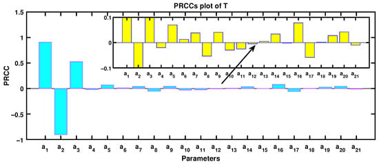
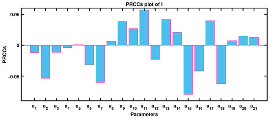
We generated 500 sets of randomly determined parameters using LHS with variations of $25\%$, utilized to compute the PRCC values for all the parameters of the model (2). The parameters were evaluated using the baseline values provided in Table 3 ( sampling performed over a range from one-tenth to twice the listed values in Table 3). The results of the sensitivity analysis with respect to tumor cell concentration T and immune cell concentration I on day 400 are shown in Figure 1 and Figure 2, respectively.

Table 3. Parameters values used for sensitivity analysis.

Parameters	Values	Reference	Parameters	Value
u	140	[26]	$a_1$	$777.77$
$k_1$	$192.8$	[26]	$a_2$	$1071.11$
$k_2$	$747.2$	[26]	$a_3$	$747.2$
$K^{-1}$	$\mathrm{10,000}$	estimated	$a_4$	$0.000093$
$k_a$	$0.18$	[24]	$a_5$	$0.01277$
$k_b$	$0.1674$	[26]	$a_6$	$\mathrm{18,950}$
$k_c$	$294.7$	[26]	$a_7$	$390.055$
$k_d$	4415	[26]	$a_8$	$\mathrm{399,722.22}$
$k_e$	$0.3411$	[26]	$a_9$	$\mathrm{844,856,193,320,378.1}$
$k_f$	$70.21$	[26]	$a_{10}$	$\mathrm{2,452,777.7}$
$k_g$	$4.172\times {10}^7$	[26]	$a_{11}$	$0.0000000104$
$k_h$	$7.195\times {10}^4$	[26]	$a_{12}$	2019
${\alpha }_1$	$3.5$	[36,37]	$a_{13}$	$0.22889$
$g_1$	100	[37]	$a_{14}$	$\mathrm{571,709.19}$
$s_d$	$1.3\times {10}^4$	[24]	$a_{15}$	$0.7552$
${\alpha }_2$	$1.36\times {10}^{-4}$	[37]	$a_{16}$	$0.003877$
$g_2$	$2.019\times {10}^7$	[24]	$a_{17}$	$0.00000373$
${\delta }_d$	$0.0412$	[24]	$a_{18}$	$\mathrm{12,273,985.15}$
$k_i$	$0.7552$	[26]	$a_{19}$	$233.80$
$k_j$	$6.979\times {10}^{-4}$	[26]	$a_{20}$	$0.00000585$
$k_k$	156	[26]	$a_{21}$	$1.055$
$k_l$	$233.8$	[26]
$k_m$	$1.053\times {10}^{-6}$	[26]
${\delta }_Z$	$0.19$	[38]

Figure 1. Sensitivity indices of the model parameters, taking the tumor cell population T as the response variable.

Figure 2. Sensitivity indices of the model parameters, taking the tumor cell population I as the response variable.

The concentration of tumor cells is most sensitive to changes in the drug input rate $\left(a_1\right)$, the maximum drug clearance rate $\left(a_2\right)$, and the drug clearance saturation $\left(a_3\right)$. We notice that T, the tumor cell concentration, is highly positively correlated with the drug input rate $\left(a_1\right)$ and the drug clearance saturation $\left(a_3\right)$, and negatively correlated with the maximum drug clearance rate $\left(a_2\right)$. Intuitively, more drug $\left(X\right)$ should suppress tumor $\left(T\right)$, but the positive PRCC of $a_1$ and $a_3$ suggests the opposite. This could be due to the harm caused by the drug $\left(X\right)$ to immune cells $\left(I\right)$, reducing immune-mediated tumor killing.

The sensitivity analysis conducted with respect to $\left(I\right)$, immune cell concentration, reveals that the death rate of immune cells by tumor cells $\left(a_7\right)$, drug-induced immunostimulatory half-saturation constant $\left(a_{15}\right)$, growth rate of immune cells due to dendritic cells $\left(a_9\right)$ and growth rate of dendritic cells due to tumor cells $\left(a_{11}\right)$ are the main parameters influencing I. As could be expected, $a_7$ and $a_{15}$ are negatively correlated with the concentration of immune cells $\left(I\right)$. The growth rate of immune cells by dendritic cells $\left(a_9\right)$ and the growth rate of dendritic cells by tumor cells $\left(a_{11}\right)$ capture the most highly positively correlated parameter. In making biological sense of the results, we note that the reaction between the dendritic cells $\left(D\right)$ and tumor cells $\left(T\right)$ results in the activation of the dendritic cells $\left(D\right)$. Furthermore, this activation results in an increase in immune cells, which the model (2) solely represents. Thus, Figure 1 and Figure 2 identify the key parameters that can guide the development of targeted treatment strategies to counteract tumor–immune evasion.

We can conclude that high-dose chemotherapy significantly damages immune cells, thereby reducing their antitumor functions. Conversely, immunotherapy enhances the proliferation of immune cells, thereby sustaining tumor suppression through the restoration of immune-mediated cytotoxicity.

4. Numerical Simulation

In this section, we present numerical simulations of our mathematical model to quantitatively analyze the dynamic interactions between tumor and immune cells during the combined effect of chemotherapy and immunotherapy. Through these computational experiments, we aim to both demonstrate the model’s theoretical predictions and provide biologically plausible interpretations of the observed dynamics.

All simulations of the mathematical model (2) and (9) were performed by MATLAB R2022a. We examine the cases when no drug (discussed in Section 2.2) and a continuous drug (discussed in Section 2.3) is applied.

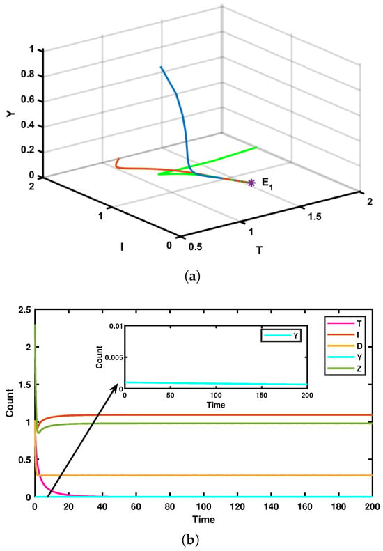
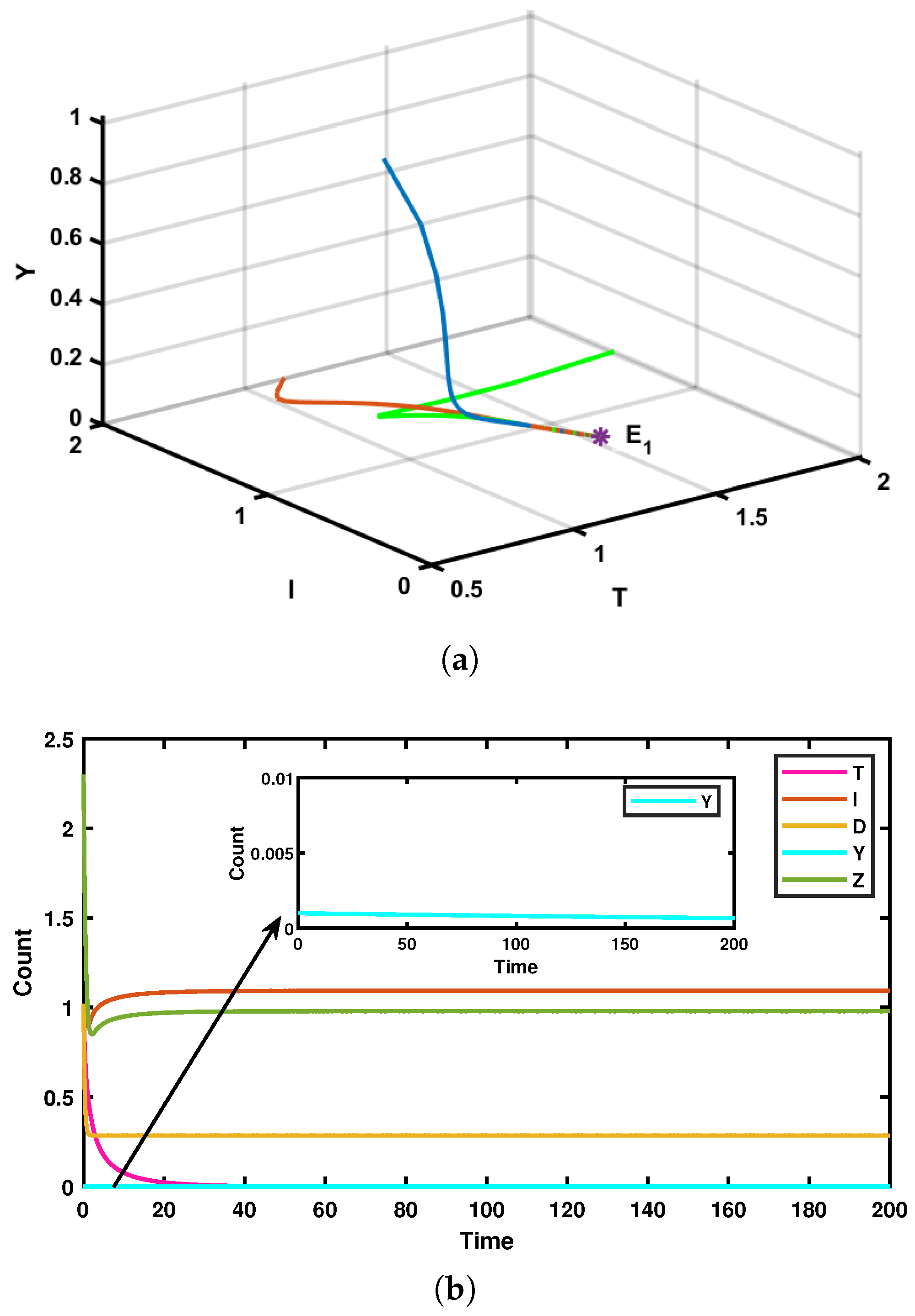
We first explore the control case when no drug is applied using assumed parameters $a_6=1.09,a_8=0.001,a_9=4.1,a_{10}=0.001,a_{11}=0.0001,a_{12}=9.2,a_{13}=3.5,a_{16}=0.001,a_{17}=0.001,a_{18}=1.9,a_{19}=1.01,a_{21}=2.1$. The numerical results demonstrate that $I_1^0=1.0928$ (satisfying $I_1^0>1$) and the condition of Theorem 3 is fulfilled. The equilibrium point $E_1$ is thereby locally asymptotically stable, as clearly illustrated in Figure 3, which presents simulation results over a 200 day period for three different initial conditions: $(1.00002,0.91,1.02,0.001,2.3)$, $(2.001,1.14,0.004,0.000051,0.3)$, and $(1.5,2.01,0.001,0.0009,1.58)$. We observe that the number of immune cells $\left(I\right)$ and dendritic cells $\left(D\right)$ decreases initially then increases up to a certain level, and later stabilizes, approaching a steady state. The density of tumor cells $\left(T\right)$ decreases significantly as immune cells $\left(I\right)$ and dendritic cells $\left(D\right)$ increase, until reaching a disease-free equilibrium $E_1$.

Figure 3. (a) For the initial conditions $(1.00002,0.91,1.02,0.001,2.3)$, $(2.001,1.14,0.004,5.1\times {10}^{-5},0.3)$, and $(1.5,2.01,0.001,0.0009,1.58)$, trajectories of solutions converge to the components of $E_1$ equilibrium. (b) Simulations of the system (9) using defined parameters as $a_{21}=2.1,a_{13}=3.5,a_6=1.09,a_8=0.001,a_9=4.1,a_{10}=0.001,a_{11}=0.0001,a_{12}=9.2,$$a_{16}=0.001,a_{17}=0.001,a_{18}=1.9,a_{19}=1.01$.

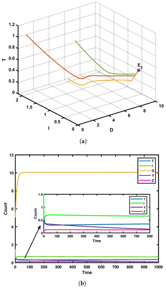
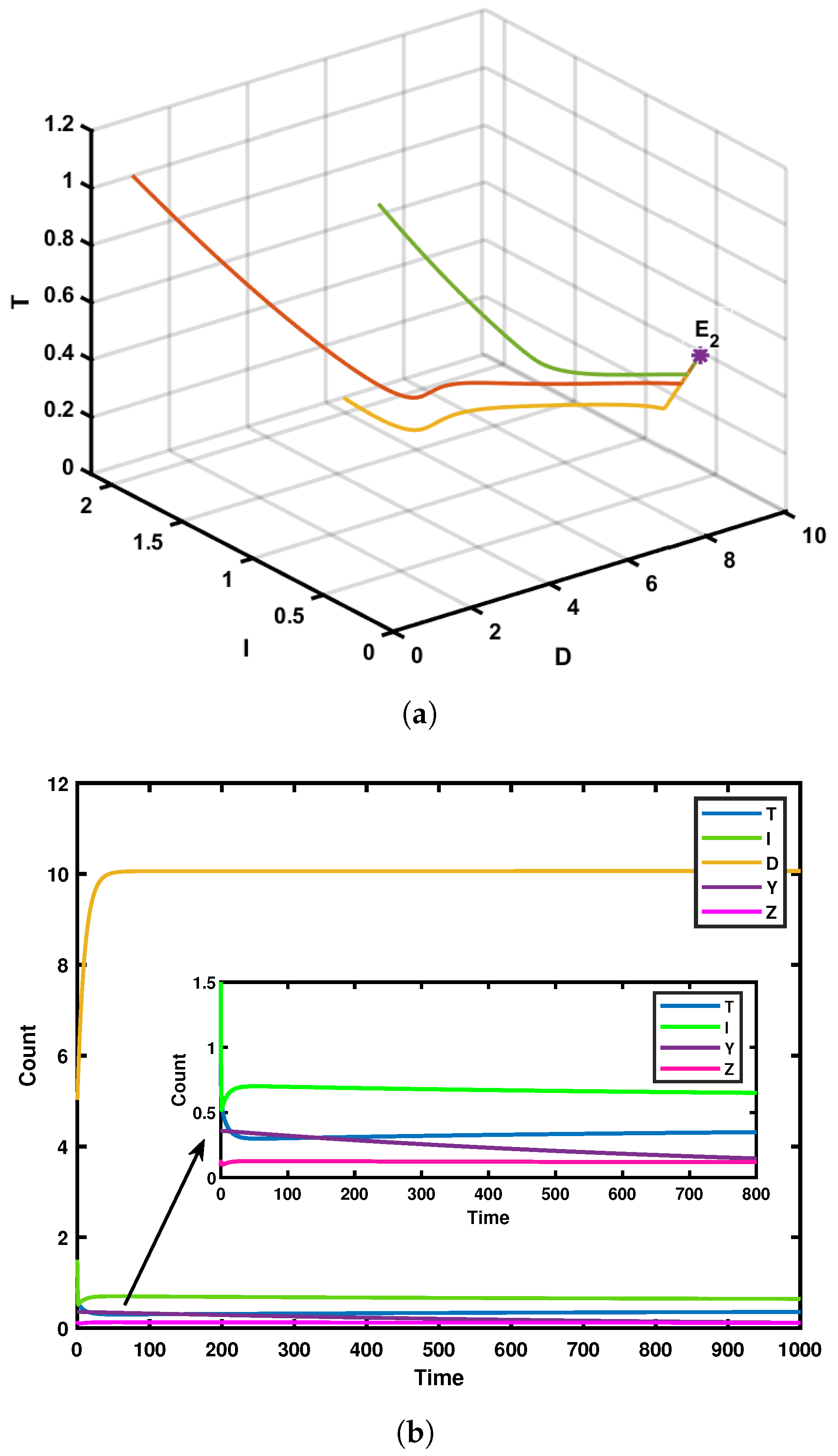
In Figure 4, we take the parameters values as $a_6=0.9,a_8=1.9,a_9=0.09,a_{10}=0.01,a_{11}=0.01,a_{12}=0.2,a_{13}=0.1,a_{16}=0.001,a_{17}=0.001,a_{18}=0.1,a_{19}=0.5,a_{21}=1.1$. It is easy to check that the following parameters satisfy the conditions for the existence and stability of the equilibrium $E_2$ stated in Theorems 5 and 6, respectively. The simulation is run for a duration of 1000 days due to slow convergence of the trajectories towards the equilibrium $E_2$ as shown in Figure 4a with initials values as $(0.9,1.5,5.03,0.36,0.09)$, $(1.001,2.14,1.04,0.52,1.3)$, and $(0.5,0.91,2.01,0.9,0.58)$. However, in Figure 4b, we discover that due to an increase in dendritic cells $\left(D\right)$, the number of immune cells $\left(I\right)$ increases, which leads to a decrease in tumors cells $\left(T\right)$, ultimately reaching a stable stationary solution $E_2$. As we know, $E_2$ is a tumorous equilibrium, although the tumor concentration decreases, it will eventually be stable at the non-zero tumor concentration. Hence, the tumor will not be eradicated in this scenario.

Figure 4. (a) The solution trajectories of system (9) converges to equilibrium $E_2$ with initial values as $(0.9,1.5,5.03,0.36,0.09)$, $(1.001,2.14,1.04,0.52,1.3)$, and $(0.5,0.91,2.01,0.9,0.58)$ along with parameters $a_{21}=1.1,a_{13}=0.1,a_6=0.9,a_8=1.9,a_9=0.09,a_{10}=0.01,a_{11}=0.01,a_{12}=0.2,a_{16}=0.001,a_{17}=0.001,a_{18}=0.1,a_{19}=0.5$. (b) Solution of the system (9) for duration of 1000 days.

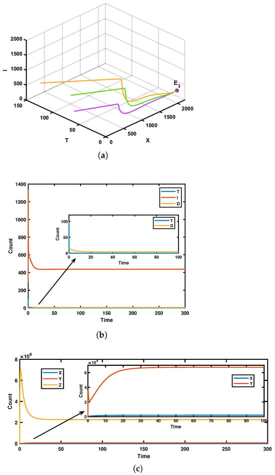
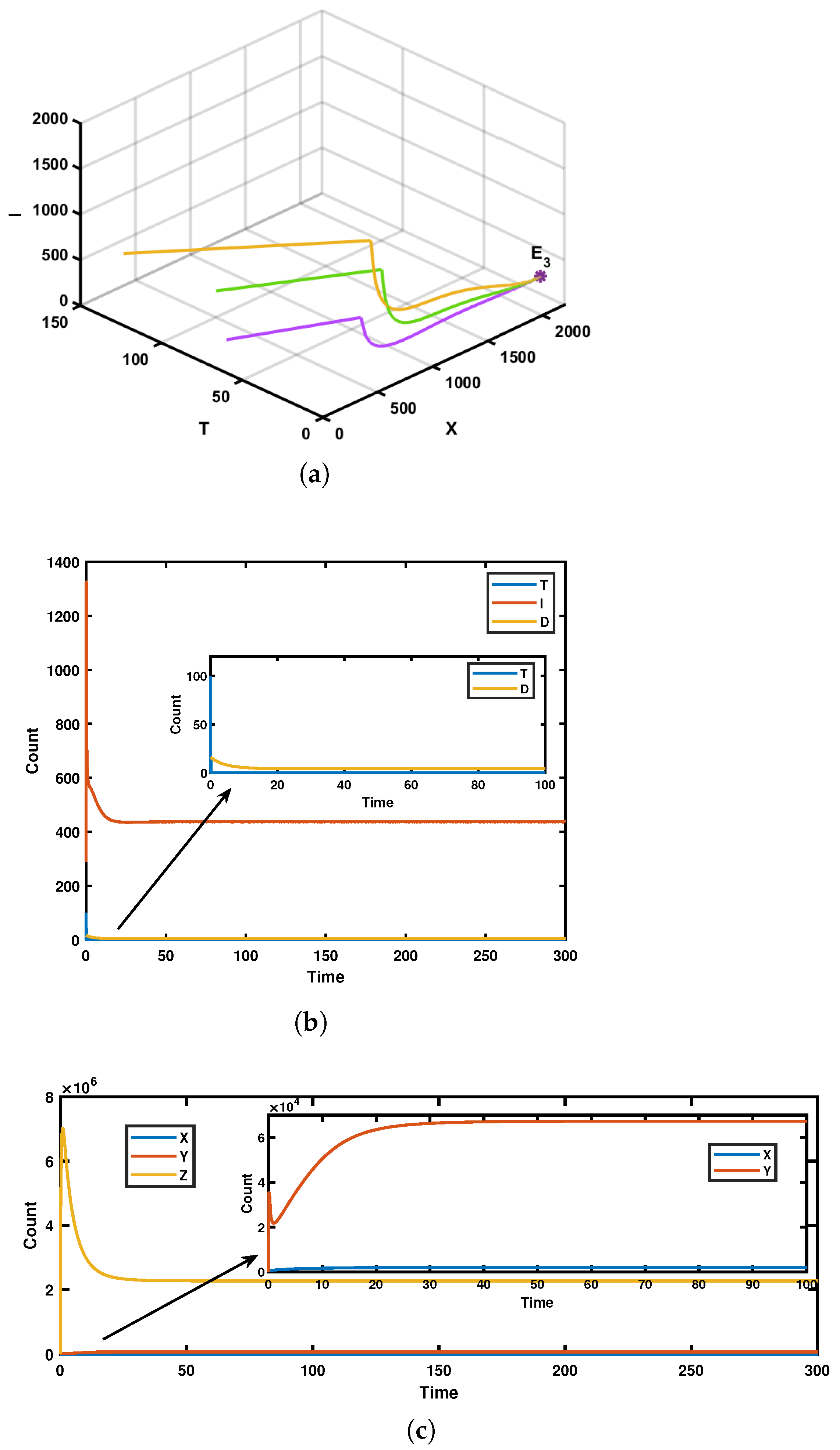
Afterwards, we examine the case of continuous drug intervention. Firstly, we discussed the tumor-free equilibrium $E_3$ of the system (9). The parameter values shown in Table 3 are used for the analysis. It is observed that these parameter values satisfy the requirements of Theorems 7 and 8. A numerical simulation was conducted over a 300-day period, using the parameters from Table 3 and along with the initial conditions $(500,100,290,16.017,0.11,2000)$, $(300,80,30,10,1.97,1000)$ and $(395,150,350,30,0.9,3000)$. As clearly illustrated in Figure 5, an increase in the immune-suppressive mediators $\left(Z\right)$ correlates with a drop in immunostimulating mediators $\left(Y\right)$. Although once Z begins to drop, Y begins to increase before reaching the state of stability. This stabilization of Y later helps stabilize immune cells $\left(I\right)$.

Figure 5. (a) The solution trajectories of the system (2) converges to tumor-free equilibrium $E_3$ with initial values as $(500,100,290,16.017,0.11,2000)$, $(300,80,30,10,1.97,1000)$ and $(395,150,350,30,0.9,3000)$. (b,c) The system solution for duration of 300 days using parameters described in Table 3.

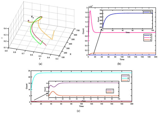
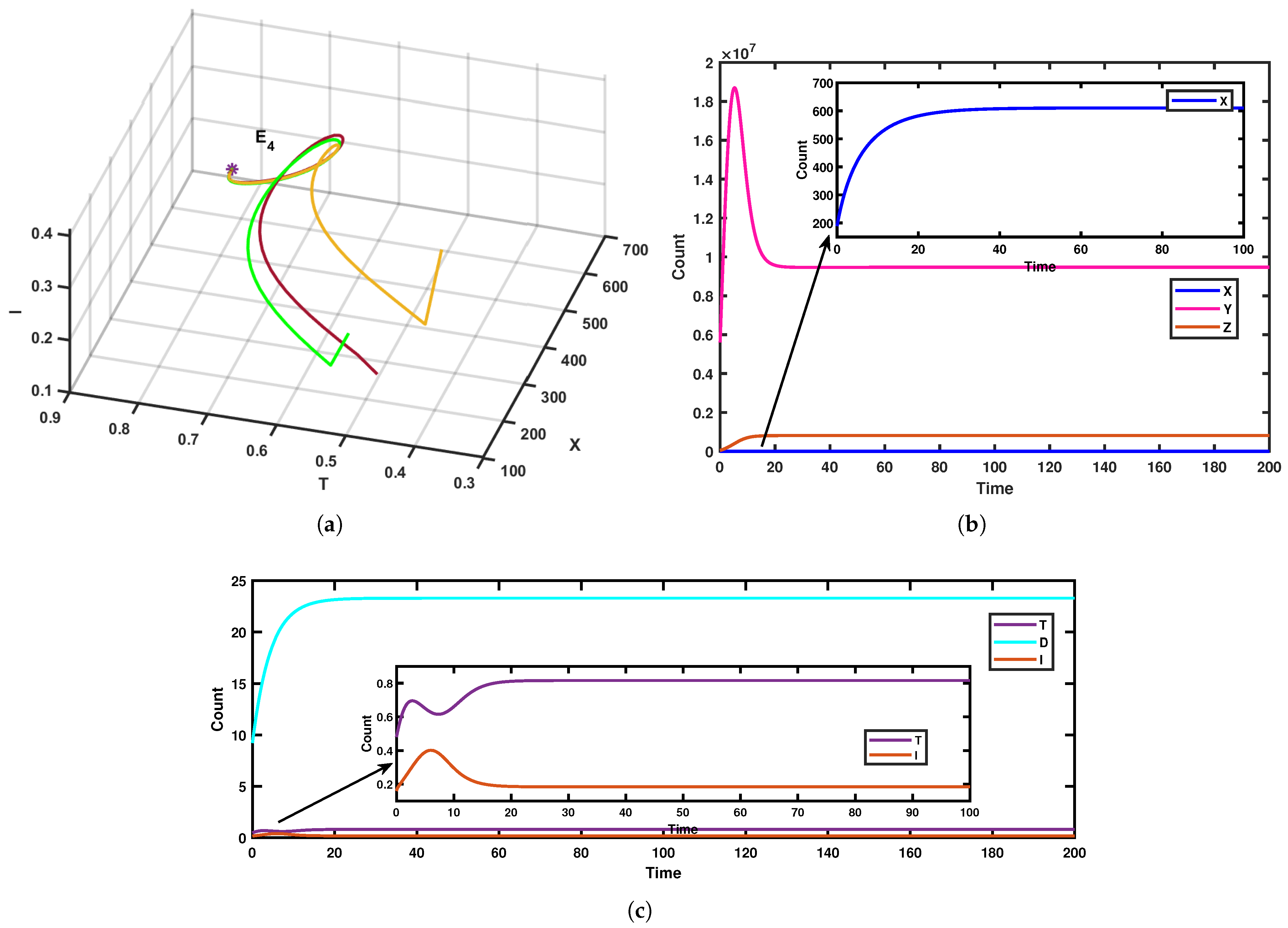
In Figure 6, we have used the parameter values from Table 4 (for the respective values of Parameters-I, we have calculated the values for Parameters-II in Table 4). It is trivial to verify that these parameters fulfill the conditions of Theorems 9 and 10. Therefore, the system (2) possesses a tumorous equilibrium $E_4$ that is asymptotically stable. This is shown in Figure 6a choosing initial conditions as $(189,0.48,0.16,9.23,5.6\times {10}^6,$ 45,000), $(150,0.51,0.26,10.5,5.9\times {10}^6,$ 49,000), and $(200,0.39,0.41,15.23,6.1\times {10}^6,$ 53,000) with 200 days of simulation time.

Figure 6. (a) The solution trajectories of the system (2) converges to tumorous equilibrium $E_4$ with initial values as $(189,0.48,0.16,9.23,5.6\times {10}^6,$ 45,000), $(150,0.51,0.26,10.5,5.9\times {10}^6,\mathrm{49,000})$, and $(200,0.39,0.41,15.23,6.1\times {10}^6,$ 53,000). (b,c) The system’s solution for duration of 200 days using parameters described in Table 4.

Table 4. Parameters values for Figure 6.

Parameters-I	Values	Reference	Parameters-II	Value
u	30	estimated	$a_1$	$166.66$
$k_1$	$52.33$	[26]	$a_2$	$290.72$
$k_2$	$454.4$	[26]	$a_3$	$454.4$
$K^{-1}$	${10}^6$	estimated	$a_4$	$3.3678\times {10}^{-7}$
$k_a$	$0.18$	[24]	$a_5$	$1.274\times {10}^{-4}$
$k_b$	$0.06062$	[26]	$a_6$	$7.8222\times {10}^7$
$k_c$	$127.4$	[26]	$a_7$	$35.7944$
$k_d$	$809.1$	[26]	$a_8$	$2.6178\times {10}^6$
$k_e$	$14.08$	[26]	$a_9$	56,125,069.44
$k_f$	$6.443$	[26]	$a_{10}$	$449.5$
$k_g$	$4.172\times {10}^7$	[26]	$a_{11}$	$4.3333$
$k_h$	$4.712\times {10}^5$	[26]	$a_{12}$	$2.00\times {10}^{-7}$
${\alpha }_1$	$0.3$	estimated	$a_{13}$	$0.2289$
$g_1$	$0.1$	estimated	$a_{14}$	5,062,424.38
$s_d$	$0.3$	estimated	$a_{15}$	$36.49$
${\alpha }_2$	$1.3$	estimated	$a_{16}$	$0.000843$
$g_2$	$0.2$	estimated	$a_{17}$	$6.2045\times {10}^{-7}$
${\delta }_d$	$0.0412$	[24]	$a_{18}$	$1.8554\times {10}^9$
$k_i$	$36.49$	[26]	$a_{19}$	6516
$k_j$	$1.518\times {10}^{-4}$	[26]	$a_{20}$	$5.6556\times {10}^{-6}$
$k_k$	$25.73$	[26]	$a_{21}$	$0.0556$
$k_l$	6516	[26]
$k_m$	$1.018\times {10}^{-6}$	[26]
${\delta }_Z$	$0.01$	estimated

Furthermore, with respect to the stated parameters, the solution of the system (2) is shown in Figure 6a,b. Observing Figure 6, we conclude that an increase in dendritic cell $\left(D\right)$ amount leads to a boost in the concentration of immune cells $\left(I\right)$. The boosted immune response reduces tumor cell $\left(T\right)$, illustrating the efficacy of dendritic cell-based immunotherapy in reducing tumor growth.

5. Conclusions

As stated in Theorem 7, the system (2), with both immunotherapy (administration of dendritic cells $\left(D\right)$) and chemotherapy, always have a tumor-free equilibrium $E_3$ if $a_2$ (rate of drug metabolism) > $a_1$ (rate of drug administration) which will be stable under certain conditions described in Theorem 8. Unlike equilibrium $E_3$, the tumorous equilibrium $E_4$ might not always exist. However, if certain conditions, as specified in Theorem 9, are satisfied, the equilibrium $E_4$ does exist and, according to Theorem 10, it may also exhibit stability. Therefore, the use of combined immuno-chemotherapy might be insufficient for achieving tumor remission or prevention. Numerical simulations further validated these findings. Overall, our quantitative analysis of the tumor–immune model highlights the critical importance of immuno-chemotherapy and its effectiveness in treatment.

Later, we performed a sensitivity analysis (using PRCC) with Latin Hypercube Sampling to determine which model parameters significantly impact tumor cell populations and immune cell concentrations. Thus, sensitivity analysis concludes that high-dose chemotherapy harms immune cells, weakening their antitumor effects, while immunotherapy boosts immune cell growth, thereby restoring tumor suppression, as explained in Section 3.

The study emphasizes the critical long-term interactions between the tumor and the immune system, avoiding sole reliance on numerical simulations. Furthermore, the stability analysis determines whether equilibria withstand perturbations, indicating that minor changes in initial conditions or treatment parameters can impact the tumor’s eradication or its ability to evade treatment. The stability analysis of the equilibrium points mentioned in this paper provides a fundamental framework for understanding the long-term behavior and resilience of dynamical systems across various scientific disciplines, including epidemiological models such as the Susceptible–Infectious–Recovered (SIR) model, ecological models, and economic theories (the Solow–Swan Growth Model), among many others.

References

- Zaver, S.A.; Woodward, J.J. Cyclic dinucleotides at the forefront of innate immunity. Curr. Opin. Cell Biol. 2020, 63, 49–56. [Google Scholar] [CrossRef] [Scilit]
- Gun, S.Y.; Lee, S.W.L.; Sieow, J.L.; Wong, S.C. Targeting immune cells for cancer therapy. Redox Biol. 2019, 25, 101174. [Google Scholar] [CrossRef] [Scilit] [PubMed]
- Gupta, I.; Hussein, O.; Sastry, K.S.; Bougarn, S.; Gopinath, N.; Chin, S.E.; Sinha, Y.; Korashy, H.M.; Maccalli, C. Deciphering the complexities of cancer cell immune evasion: Mechanisms and therapeutic implications. Adv. Cancer Biol. Metastasis 2023, 8, 100107. [Google Scholar] [CrossRef] [Scilit]
- Erasha, A.M.; El-Gendy, H.; Aly, A.S.; Fernández-Ortiz, M.; Sayed, R.K. The role of the tumor microenvironment (TME) in advancing cancer therapies: Immune system interactions, tumor-infiltrating lymphocytes (TILs), and the role of exosomes and inflammasomes. Int. J. Mol. Sci. 2025, 26, 2716. [Google Scholar] [CrossRef] [Scilit] [PubMed]
- Zhu, Y.; Knolhoff, B.L.; Meyer, M.A.; Nywening, T.M.; West, B.L.; Luo, J.; W. Gillam, A.; Goedegebuure, S.P.; Linehan, D.C.; DeNardo, D.G. CSF1/CSF1R blockade reprograms tumor-infiltrating macrophages and improves response to T-cell checkpoint immunotherapy in pancreatic cancer models. Cancer Res. 2014, 74, 5057–5069. [Google Scholar] [CrossRef] [Scilit]
- Malek, E.; De Lima, M.; Letterio, J.J.; Kim, B.G.; Finke, J.H.; Driscoll, J.J.; Giralt, S.A. Myeloid-derived suppressor cells: The green light for myeloma immune escape. Blood Rev. 2016, 30, 341–348. [Google Scholar] [CrossRef] [Scilit] [PubMed]
- Dougan, M.; Dranoff, G. Immune therapy for cancer. Annu. Rev. Immunol. 2009, 27, 83–117. [Google Scholar] [CrossRef] [Scilit]
- Barber, F.D. Adverse events of oncologic immunotherapy and their management. Asia Pac. J. Oncol. Nurs. 2019, 6, 212–226. [Google Scholar] [CrossRef] [Scilit]
- Engleman, E.G. Dendritic cell–based cancer immunotherapy. Semin. Oncol. 2003, 30, 23–29. [Google Scholar] [CrossRef] [Scilit]
- Osada, T.; Clay, T.M.; Woo, C.Y.; Morse, M.A.; Lyerly, H.K. Dendritic cell-based immunotherapy. Int. Rev. Immunol. 2006, 25, 377–413. [Google Scholar] [CrossRef] [Scilit]
- Alatrash, G.; Jakher, H.; Stafford, P.D.; Mittendorf, E.A. Cancer immunotherapies, their safety and toxicity. Expert Opin. Drug Saf. 2013, 12, 631–645. [Google Scholar] [CrossRef] [Scilit]
- Rak, A.M.; Telejko, I.; Adamczuk, G.; Trombik, T.; Stepulak, A.; Błaszczak, E. Advancing Head and Neck Cancer Therapies: From Conventional Treatments to Emerging Strategies. Biomedicines 2025, 13, 1046. [Google Scholar] [CrossRef] [Scilit]
- Lv, X.; Zhang, P.B.; Zhang, E.; Yang, S. Predictive factors and prognostic models for Hepatic arterial infusion chemotherapy in Hepatocellular carcinoma: A comprehensive review. World J. Surg. Oncol. 2025, 23, 1–24. [Google Scholar] [CrossRef] [Scilit]
- Kogan, Y.; H. Tobias, K.; Elishmereni, M.; V. Pavlović, S.; Agur, Z. Reconsidering the paradigm of cancer immunotherapy by computationally aided real-time personalization. Cancer Res. 2012, 72, 2218–2227. [Google Scholar] [CrossRef] [Scilit]
- DePillis, L.G.; Eladdadi, A.; Radunskaya, A.E. Modeling cancer-immune responses to therapy. J. Pharmacokinet. Pharmacodyn. 2014, 41, 461–478. [Google Scholar] [CrossRef] [Scilit] [PubMed]
- Bellomo, N.; Preziosi, L. Modelling and mathematical problems related to tumor evolution and its interaction with the immune system. Math. Comput. Model. 2000, 32, 413–452. [Google Scholar] [CrossRef] [Scilit]
- Liu, P.; Liu, X. Dynamics of a tumor-immune model considering targeted chemotherapy. Chaos Solitons Fractals 2017, 98, 7–13. [Google Scholar] [CrossRef] [Scilit]
- Mahlbacher, G.E.; Reihmer, K.C.; Frieboes, H.B. Mathematical modeling of tumor-immune cell interactions. J. Theor. Biol. 2019, 469, 47–60. [Google Scholar] [CrossRef] [Scilit]
- Kumar, A.; Dubey, U.S.; Dubey, B. The impact of radio-chemotherapy on tumour cells interaction with optimal control and sensitivity analysis. Math. Biosci. 2024, 369, 109146. [Google Scholar] [CrossRef] [Scilit] [PubMed]
- Xu, Q.; Fan, A.; Qu, L.; Miao, Y.; Du, L. Stability switch of tumor-immune system driven by delayed response in cell-to-cell contact. Eur. Phys. J. Spec. Top. 2025, 234, 165–178. [Google Scholar] [CrossRef] [Scilit]
- Qomlaqi, M.; Bahrami, F.; Ajami, M.; Hajati, J. An extended mathematical model of tumor growth and its interaction with the immune system, to be used for developing an optimized immunotherapy treatment protocol. Math. Biosci. 2017, 292, 1–9. [Google Scholar] [CrossRef] [Scilit]
- Pang, L.; Liu, S.; Zhang, X.; Tian, T. Mathematical modeling and dynamic analysis of anti-tumor immune response. J. Appl. Math. Comput. 2020, 62, 473–488. [Google Scholar] [CrossRef] [Scilit]
- DePillis, L.G.; Radunskaya, A.E.; Wiseman, C.L. A validated mathematical model of cell-mediated immune response to tumor growth. Cancer Res. 2005, 65, 7950–7958. [Google Scholar] [CrossRef] [Scilit]
- Kuznetsov, V.A.; Makalkin, I.A.; Taylor, M.A.; Perelson, A.S. Nonlinear dynamics of immunogenic tumors: Parameter estimation and global bifurcation analysis. Bull. Math. Biol. 1994, 56, 295–321. [Google Scholar] [CrossRef] [Scilit] [PubMed]
- d’Onofrio, A. A general framework for modeling tumor-immune system competition and immunotherapy: Mathematical analysis and biomedical inferences. Phys. D Nonlinear Phenom. 2005, 208, 220–235. [Google Scholar] [CrossRef] [Scilit]
- Tran, A.P.; Radhawi, M.A.; Kareva, I.; Wu, J.; Waxman, D.J.; Sontag, E.D. Delicate balances in cancer chemotherapy: Modeling immune recruitment and emergence of systemic drug resistance. Front. Immunol. 2020, 11, 1376. [Google Scholar] [CrossRef] [Scilit] [PubMed]
- Diebner, H.H.; Zerjatke, T.; Griehl, M.; Roeder, I. Metabolism is the tie: The Bertalanffy-type cancer growth model as common denominator of various modelling approaches. Biosystems 2018, 167, 1–23. [Google Scholar] [CrossRef] [Scilit]
- Nikolopoulou, E.; Johnson, L.; Harris, D.; Nagy, J.; Stites, E.; Kuang, Y. Tumour-immune dynamics with an immune checkpoint inhibitor. Lett. Biomath. 2018, 5, S137–S159. [Google Scholar] [CrossRef]
- Guiot, C.; Delsanto, P.P.; Carpinteri, A.; Pugno, N.; Mansury, Y.; Deisboeck, T.S. The dynamic evolution of the power exponent in a universal growth model of tumors. J. Theor. Biol. 2006, 240, 459–463. [Google Scholar] [CrossRef] [Scilit]
- Castañeda, A.R.S.; Torres, E.R.; Goris, N.A.V.; González, M.M.; Reyes, J.B.; González, V.S.; Schonbek, M.; Montijano, J.I.; Cabrales, L.E.B. New formulation of the Gompertz equation to describe the kinetics of untreated tumors. PLoS ONE 2019, 14, e0224978. [Google Scholar] [CrossRef] [Scilit]
- Murphy, H.; Jaafari, H.; Dobrovolny, H.M. Differences in predictions of ODE models of tumor growth: A cautionary example. BMC Cancer 2016, 16, 163. [Google Scholar] [CrossRef] [Scilit]
- Gunnarsson, E.B.; Kim, S.; Choi, B.; Schmid, J.K.; Kaura, K.; Lenz, H.J.; Mumenthaler, S.M.; Foo, J. Understanding patient-derived tumor organoid growth through an integrated imaging and mathematical modeling framework. PLoS Comput. Biol. 2024, 20, e1012256. [Google Scholar] [CrossRef] [Scilit]
- Marino, S.; Hogue, I.B.; Ray, C.J.; Kirschner, D.E. A methodology for performing global uncertainty and sensitivity analysis in systems biology. J. Theor. Biol. 2008, 254, 178–196. [Google Scholar] [CrossRef] [Scilit] [PubMed]
- McKay, M.D.; Beckman, R.J.; Conover, W.J. A comparison of three methods for selecting values of input variables in the analysis of output from a computer code. Technometrics 1979, 21, 239–245. [Google Scholar]
- Stein, M. Large sample properties of simulations using Latin hypercube sampling. Technometrics 1987, 29, 143–151. [Google Scholar] [CrossRef]
- Friedman, A.; Hao, W. The role of exosomes in pancreatic cancer microenvironment. Bull. Math. Biol. 2018, 80, 1111–1133. [Google Scholar] [CrossRef] [Scilit] [PubMed]
- Sardar, M.; Khajanchi, S.; Biswas, S.; Ghosh, S. A mathematical model for tumor-immune competitive system with multiple time delays. Chaos Solitons Fractals 2024, 179, 114397. [Google Scholar] [CrossRef] [Scilit]
- Anderson, H.G.; Takacs, G.P.; Harris, D.C.; Kuang, Y.; Harrison, J.K.; Stepien, T.L. Global stability and parameter analysis reinforce therapeutic targets of PD-L1-PD-1 and MDSCs for glioblastoma. J. Math. Biol. 2024, 88, 10. [Google Scholar] [CrossRef] [Scilit]
Disclaimer/Publisher’s Note: The statements, opinions and data contained in all publications are solely those of the individual author(s) and contributor(s) and not of MDPI and/or the editor(s). MDPI and/or the editor(s) disclaim responsibility for any injury to people or property resulting from any ideas, methods, instructions or products referred to in the content. |
© 2026 by the authors. Licensee MDPI, Basel, Switzerland. This article is an open access article distributed under the terms and conditions of the Creative Commons Attribution (CC BY) license.