Application of a Reinforcement Learning-Based Improved Genetic Algorithm in Flexible Job-Shop Scheduling Problems

Abstract

This paper addresses the limitations of genetic algorithms in solving the Flexible Job-Shop Scheduling Problem (FJSP) including slow convergence, susceptibility to local optima, and sensitivity to parameter settings. The paper proposes an Improved Genetic Algorithm based on Reinforcement Learning (IGARL). First, a hybrid population selection mechanism that combines the Queen Bee Mating Flight (QBMF) strategy with the Tournament Selection (TS) method is introduced. This mechanism significantly accelerates convergence by optimizing the population structure. Second, a dynamic population update strategy based on tunnel vision, termed the Solution Space Diversity Awakening (SSDA) strategy, is developed. When the population becomes trapped in local optima, this strategy intelligently triggers random perturbations and introduces high-potential individuals to enhance the algorithm’s ability to escape local optima and promote population diversity. Third, a novel multi-Q-table reinforcement learning framework is embedded within the iterative process to dynamically adjust key genetic algorithm parameters (such as selection, mutation, and crossover rates) and enable multi-dimensional performance evaluation, thereby effectively guiding the search toward better solutions. Experimental results demonstrate that the IGARL algorithm achieves a 10% to 60% improvement in convergence speed on Brandimarte benchmark instances, with solution quality significantly surpassing that of the basic genetic algorithm. Moreover, the fluctuation of the average optimal solution remains within 20%, indicating strong stability and robustness.

1. Introduction

The manufacturing industry, as a vital pillar of the international economy, has production efficiency and cost control that are directly linked to a world’s economic development. The Job-Shop Scheduling Problem (JSP) is a critical combinatorial optimization challenge in manufacturing, aiming to efficiently schedule a set of processing tasks using limited resources to maximize production efficiency. JSP has been proven to be NP-hard [1], indicating that the computational difficulty of finding an optimal solution increases exponentially as the problem size grows. The inherent complexity and dynamic stochastic nature of JSP highlight the necessity of developing efficient and accurate solution approaches.

The Flexible Job-Shop Scheduling Problem (FJSP) [2], as an extension of the classical Job-Shop Scheduling Problem (JSP), introduces greater flexibility and complexity. In FJSP, each operation of a job can be processed on any available machine, which not only increases the complexity of decision-making but also requires the algorithm to consider both operation sequencing and machine selection simultaneously. With the rapid growth in demand for customized production, the traditional JSP with its fixed machine assignments has become increasingly inadequate for the flexible reuse of equipment in practical manufacturing. FJSP enables dynamic selection of machines among multiple compatible options for each operation, significantly improving resource utilization and production efficiency, thus becoming a key optimization issue in intelligent manufacturing. For example, FJSP is of significant research and practical value in the production of power tools, where factories manufacture various products such as electric drills, rotary hammers, angle grinders, and cutting machines. In such settings, customer demands are diverse, product life cycles are short, orders are dynamically changing, and different products have unique assembly and process requirements. Each operation can be performed on multiple types of equipment, resulting in increasing complexity in planning, process allocation, and resource scheduling. Manual scheduling under these conditions is challenging, inefficient, and leads to low resource utilization. By optimizing scheduling through FJSP, it is possible to arrange the sequence and machine assignment of each process step according to equipment status and order requirements, thereby improving equipment utilization, reducing idle time, shortening production cycles, increasing production efficiency and flexibility, meeting market needs for product diversity and customization, and ultimately enhancing the competitiveness of enterprises.

For the Flexible Job-Shop Scheduling Problem (FJSP), researchers have proposed various solution methods, including genetic algorithms [3], gray wolf optimizers [4], ant colony algorithms [5], and other swarm intelligence-based algorithms [2]. These approaches have improved the efficiency and quality of solutions for scheduling problems to varying degrees. For example, a two-level particle swarm optimization algorithm was introduced by [6] to reduce both solution evaluations and objective function calculations in the FJSP. An improved gray wolf optimizer to deal with the flexible job-shop scheduling problem was proposed by [7] using a random key for coding job positions and adopting a local search strategy. Ref. [8] introduced a sparrow search algorithm for FJSP, modifying the encoding and decoding schemes specifically for this problem, and demonstrated its feasibility on standard benchmark instances. Ref. [9] developed an enhanced cuckoo search algorithm for dual-resource constrained FJSP by partitioning the population into three subgroups and facilitating information exchange through a differential operator, thereby improving both local and global search abilities. Ref. [10] developed a hybrid strategy that merges genetic algorithms with Tabu search to boost solution effectiveness, while [11] strengthened the local search ability of the bee colony optimization (BCO) algorithm by introducing adaptive mechanisms. Ref. [12] combines the local search ability of simulated annealing algorithm and the global search ability of genetic algorithm, which has been successfully applied to FJSP [13].

With the advancement of artificial intelligence technologies, deep learning and reinforcement learning methods [14,15] have also been applied to the study of the Flexible Job-Shop Scheduling Problem (FJSP). Ref. [16] integrated reinforcement learning with genetic algorithms to optimize school bus scheduling, achieving reductions in both travel distance and time. Ref. [17] developed a test case prioritization algorithm that leverages both reinforcement learning and genetic algorithms, demonstrating superior performance compared to traditional approaches. Ref. [18] addressed the challenge that intelligent algorithms cannot effectively adjust key parameters in FJSP by proposing a Self-Learning Genetic Algorithm (SLGA), which employs a genetic algorithm as the primary optimization approach and uses reinforcement learning (RL) to intelligently adjust its key parameters. Ref. [19] addressed the FJSP by designing a neighborhood genetic algorithm that maintains population diversity through the use of dynamic crossover probabilities. Ref. [20] proposed a non-dominated genetic algorithm with an elite strategy, wherein dynamic crossover and mutation probabilities are determined based on the non-domination rank and iteration count. However, due to the large and complex state and action spaces, highly dynamic environments, and sparse reward signals, most deep reinforcement learning algorithms still face challenges when solving FJSP, such as slow convergence, a high number of iterations, susceptibility to local optima, and difficulty in obtaining optimal solutions within a limited number of training episodes.

Building on previous research, this paper proposes an Improved Genetic Algorithm based on Deep Reinforcement Learning (IGARL) [21]. The algorithm incorporates an active selection mechanism inspired by queen bee mating behavior. By dynamically adjusting the search direction or resource allocation strategy through the Queen Bee Mating Flight (QBMF) Strategy, the algorithm ensures efficient optimization and accelerates convergence. Additionally, a solution space diversity activation strategy is introduced, which retains a portion of the best-fit chromosomes while re-initializing the remaining chromosomes. This approach enables the algorithm to avoid getting trapped in local optima, thereby improving the overall search quality and facilitating the discovery of superior solutions. Leveraging reinforcement learning techniques, IGARL can intelligently adjust key parameters such as population selection rate, crossover probability, and mutation probability. The algorithm also evaluates states from three perspectives: average population fitness, optimal fitness, and population diversity, thereby improving overall scheduling performance. Experimental validation using Brandimarte benchmark instances demonstrates that the proposed algorithm excels in both computational efficiency and the ability to escape local optima, achieving superior results compared to several existing algorithms. This study not only improves the efficiency and quality of FJSP solutions but also provides new approaches and methodologies for practical production scheduling.

Genetic Algorithm (GA) is selected as the foundational framework for this study due to its effectiveness and flexibility in solving combinatorial optimization problems. However, its inherent limitations such as slow convergence, susceptibility to local optima, and parameter sensitivity restrict its performance. To address these issues, reinforcement learning is introduced to enable dynamic, adaptive adjustment of key parameters, balancing exploration and exploitation. Furthermore, the Queen Bee Mating Flight (QBMF) strategy is innovatively proposed to accelerate convergence and the Solution Space Diversity Awakening (SSDA) strategy to actively escape local optima, thus forming the unique IGARL algorithm.

In contrast, existing methods face significant limitations for this study. Exact methods like mathematical programming are computationally prohibitive for large-scale FJSP instances, while pure heuristic rules provide limited optimization. Other metaheuristics such as Particle Swarm Optimization and Ant Colony Optimization encounter challenges in parameter tuning and local optima, whereas the Genetic Algorithm framework better accommodates our proposed strategies. Pure deep reinforcement learning methods, including Actor-Critic and Proximal Policy Optimization, often suffer from complex state spaces and slow convergence in FJSP contexts. Comparatively, our hybrid approach integrating Q-learning/SARSA with GA maintains adaptability while being more lightweight and efficient—advantages confirmed by its superior experimental performance.

The structure of this paper is organized as follows: Chapter 2 describes the Flexible Job-Shop Scheduling Problem (FJSP) and establishes its mathematical model. Chapter 3 details the proposed Improved Genetic Algorithm based on Reinforcement Learning (IGARL), including its basic GA framework, the Queen Bee Mating Flight (QBMF) strategy, the Solution Space Diversity Awakening (SSDA) strategy, and the reinforcement learning parameter adjustment mechanism based on multiple Q-tables. Chapter 4 presents the experimental design and results analysis, including the validation of the effectiveness of each improvement strategy and a comparison between IGARL and existing state-of-the-art algorithms. Chapter 5 concludes the paper and outlines future research directions.

2. Flexible Job-Shop Scheduling Model

2.1. Problem Description

The Flexible Job-Shop Scheduling Problem (FJSP) is defined as follows: Given n jobs to be processed on m machines, each job comprises a specific sequence of operations, with the number of operations potentially differing across jobs. Each operation Oij (the j-th operation of job i) can be assigned to any machine from its eligible set, and the processing time for each operation may vary depending on the chosen machine. The goal is to determine both the optimal sequence of operations for all jobs and the assignment of each operation to a suitable machine, in order to minimize the makespan, which is the maximum completion time. Thus, the FJSP can be divided into two sub problems: sequencing the operations and selecting the machines for each operation [22]. The problem must also adhere to the following constraints.

(1)

At zero hours, all jobs can be processed.

(2)

Each job has an equal priority.

(3)

Each machine can process only one operation at a time.

(4)

Only one machine can be selected for the same workpiece at the same time, and once the machine is selected, the machine cannot be changed until the current process is complete.

(5)

The processing time for each operation differs across machines and is known in advance, as presented in Table 1.

Table 1. The operational processing schedule.

Jobs	Process	M1	M2	M3	M4	M5	M6
J1	O11	3	4	6	4	5	-
	O12	2	7	-	3	-	2
	O13	5	3	-	4	8	3
J2	O21	-	5	9	5	-	5
	O22	4	6	8	-	6	4
	O23	3	4	5	7	3	4

(6)

There is a precedence constraint on the processing order of the same job operation.

2.2. Mathematical Model

The definitions of the parameters for the FJSP are shown in Table 2.

Table 2. FJSP model parameters.

Parameter	Description
n	Total number of jobs; set of jobs J = {J1, J2, J3, …, Jn}
m	Total number of machines; set of machines M = {M1, M2, M3, …, Mm}
hi	Total number of operations for the i-th job, i = 1, 2, 3, …, n
Oij	The j-th operation of the job i
Sij	Start time of the j-th operation of job i
Fij	Finish time of the j-th operation of job i
Tijk	The time it takes machine k to complete the j-th operation of job i, k = 1, 2, 3, …, m
Xijk	Equals 1 if operation Oij is processed on machine k; otherwise equals 0
Xijpqk	Equals 1 if, on machine k, operation Oij is processed prior to operation Opq; otherwise equals 0
Cmax	minimizing the makespan, $C_{\mathrm{m}\mathrm{a}\mathrm{x}}=min\{\mathrm{m}\mathrm{a}\mathrm{x}{C}_i,i=\mathrm{1,2},...,n\}$

3. IGARL Algorithm for Solving the FJSP

3.1. Basic Genetic Algorithm

The basic genetic algorithm is an optimization technique modeled after the concepts of natural selection and genetic inheritance. It operates by initializing a random population, evaluating individual fitness, selecting superior individuals, performing crossover and mutation operations, and iteratively updating the population to progressively approach the optimal or near-optimal solution.

A straightforward encoding scheme can effectively represent the relationship between chromosomes and feasible solutions, ensuring the validity of the encoding. Therefore, the MSOS encoding method [18] is adopted in this study. Each chromosome consists of a machine selection string (MS) and an operation sequence string (OS) [23,24,25], where each chromosome corresponds to a feasible solution to the problem.

In this study, the population is initialized by using the GLR (Global selection, Local selection, and Random selection) hybrid initialization method [26]. Adjusting the proportions of the initialized population is analogous to balancing exploration and exploitation in reinforcement learning. For example, appropriately increasing the proportion of exploratory individuals encourages the algorithm to search more extensively within the solution space, thereby avoiding local optima. Conversely, increasing the proportion of exploitative individuals can accelerate convergence in regions with high-quality solutions, helping to avoid local optima or premature convergence. When the solution space is large or the problem is complex, the proportion of randomly generated individuals can be increased to enhance exploration. For simpler problems or when strong prior knowledge is available, increasing the proportion of high-quality individuals can accelerate convergence. Experimental results indicate that when the proportions of GS/LS/RS are set to 6:3:1 [26], the initial optimal solution became better, and convergence occurred more rapidly. The fitness function serves as the criterion for evaluating the quality of individuals. Considering the characteristics of the FJSP, the objective is to minimize the maximum completion time, i.e., to minimize the makespan. Therefore, the reciprocal of the maximum completion time used as the fitness function, specifically the reciprocal of the objective function $C_{\mathrm{m}\mathrm{a}\mathrm{x}}$. Thus, the fitness value of an individual defined as $f={\displaystyle \frac{1}{C_{\mathrm{m}\mathrm{a}\mathrm{x}}}}$. A larger value of f indicates a shorter makespan and consequently higher fitness.

The crossover operation refers to generating new offspring chromosomes from two parent chromosomes through specific operations to preserve advantageous genes. For the operation sequence component, the Partially Matched Crossover (POX) [18] method is utilized, whereas a two-point crossover is applied to the machine assignment component. In the two-point crossover, two positions are randomly chosen as crossover points, and the segments between these points are swapped between the chromosomes.

Mutation is essential for preserving population diversity and avoiding premature convergence to local optima. The mutation probability determines the likelihood that each gene or individual will undergo mutation in each generation. This probability is a real number between 0 and 1, and it can be either fixed or adaptively adjusted during the evolutionary process [27,28].

3.2. Improved Genetic Algorithm

3.2.1. Queen Bee Mating Flight Strategy

The basic genetic algorithm often suffers from slow convergence and a large number of iterations, necessitating further improvement. In this study, the Queen Bee Mating Flight strategy (QBMF) is adopted, which draws on the queen bee’s proactive selection mechanism during mating flights to maintain population quality and address the issues of slow convergence and excessive iterations.

Specifically, in nature, the queen bee releases pheromones during her mating flight to attract drones, which form a drone congregation to pursue her. The queen mates with multiple drones typically around 15 in a single flight to produce offspring, a phenomenon known as queen bee mating flight. The integration and application of the queen bee mating flight mechanism with traditional scheduling are summarized in Table 3. In dynamic scheduling, the “Queen Bee Mating Flight Strategy” refers to adopting the queen bee’s active selection behavior, dynamically adjusting the search direction or resource allocation rules to ensure algorithmic optimization efficiency and improve convergence speed.

Table 3. Integration and Application Analysis of QBMF and Traditional Scheduling.

Areas/Aspects	Traditional Strategy	QBMF	Application Scenario
Path Selection	Fixed search path	Dynamic path selection	Logistic route optimization
Resource Allocation	Uniform resource distribution	Dynamic allocation based on capacity/load	Cloud computing task scheduling
Diversity	Lack of diversity preservation	Enforced retention of suboptimal solutions to prevent premature convergence	Combinatorial optimization problems

The following describes the core mechanism of the QBMF in dynamic scheduling. In task allocation or resource scheduling, a competitive mechanism is introduced, allowing nodes (such as servers or vehicles) to actively select tasks based on real-time load or capability, rather than receiving passive assignments. For instance, nodes with lower loads can “actively attract” more tasks, analogous to the queen bee attracting drones. In genetic algorithms, the selection operation can retain chromosomes with higher fitness, ensuring optimization efficiency and accelerating convergence.

In this study, the QBMF is employed to perform additional crossover operations on the population. Specifically, in each iteration of the genetic algorithm, the chromosome with the highest fitness (the queen bee) is selected to perform crossover and mutation operations with 15 other chromosomes (drones) in the population, generating 15 new offspring. The newly generated individuals, along with those produced through standard crossover and mutation, are ranked according to their fitness. To preserve the original population size for the next iteration, the 15 individuals with the lowest fitness are removed.

Why it is 15 drones is based on the bionic principles and systematic parameter sensitivity analysis as shown in Table 4: In a natural bee colony, the queen typically mates with 10 to 20 drones during a single nuptial flight to achieve optimal genetic diversity which supports QBMF to take this scope as starting point. The experiment’s result shows that when the number of drones is set to 15, the algorithm achieves the lowest average makespan (Ave_Cmax = 69.30) with a relatively small standard deviation (SD_Cmax = 1.03), indicating that this configuration strikes the best balance between exploration capability and convergence stability. Therefore, in all subsequent comparative experiments, the number of drones is fixed at 15.

Table 4. Parameter sensitivity analysis on drones’ quantity.

#	QTY of Drones	Min	Max	Ave_Cmax	SD_Cmax
1	10	68	71	70.00	0.94
2	11	67	71	69.90	1.72
3	12	69	71	70.10	0.74
4	13	68	72	70.50	1.18
5	14	68	72	69.80	1.23
6	15	67	71	69.30	1.03
7	16	69	73	71.10	1.29
8	17	70	73	71.40	1.07
9	18	69	75	70.70	1.89
10	19	67	72	70.40	1.71
11	20	68	74	71.00	2.05

The complete procedure of QBMF is outlined in below Algorithm 1.

Algorithm 1: QBMF

1:    begin

2:    Pf is the probability of the queen bee mating flight strategy.

3:    Pc is the probability of the crossover strategy.

4:    Pm is the probability of the mutation strategy.

5:    initialize offspring

6:    if random < Pf then

7:          Within the population, the chromosome exhibiting the highest fitness is designated as the Queen Bee.

8:            Fifteen chromosomes randomly selected from the population as Drones.

9:            for i from 1 to 15 do

10:                        if random < Pc then

11:                                Perform crossover on Queen Bee and Drones[i] to generate new chromosomes.

12:                            the new chromosome added to offspring.

13:                    else

14:                            Queen Bee and Drones[i] serve as the new chromosomes.

15:                    end if

16:                    if random < Pm then

17:                            Mutate the new chromosome

18:                            the new chromosome added to offspring

19:                    end if

20:            end for

21:    end if

The introduction of QBMF employs probability P_f to favor the selection of high-quality individuals, which enhances convergence speed but also intensifies selection pressure. This may accelerate the loss of population diversity and lead to premature convergence. Such risks are particularly pronounced when P_f is set too high, when combined with a high crossover rate P_c and a low mutation rate P_m, or when the individual quality evaluation metric stagnates. To mitigate this effect, this study utilizes a reinforcement learning module to dynamically and collaboratively adjust P_f, P_c and P_m. By monitoring indicators such as population diversity decline or abnormal convergence trends, the system adaptively reduces P_f or increases P_m, thereby achieving an effective balance between intensified selection and global exploration and avoiding premature convergence.

3.2.2. Solution Space Diversity Activation Strategy

Although genetic algorithms are theoretically capable of global search, they may still become trapped in local optima, particularly when population diversity is insufficient—an issue known as the tunnel vision phenomenon. Tunnel vision refers to a specific visual condition where, due to the constraints of tunnel walls, an individual field of vision significantly reduced. Under normal circumstances, a person’s horizontal visual field can reach 180° or wider; however, in a tunnel, the visible angle may be reduced to just a few dozen degrees. For example, when a car enters a tunnel, the driver can see only the tunnel’s interior walls and lighting, while the view of the distant exterior is obstructed, making it difficult to perceive the broader landscape outside the tunnel.

In dynamic scheduling, focusing solely on local optimization can lead to overlooking the interdependencies among different part of the system. For instance, in the dynamic scheduling of a production workshop, optimizing only a single process’s efficiency without considering preceding and subsequent processes, as well as the supply of raw materials and inventory of finished products, is analogous to tunnel vision ignoring the larger context of the road network outside the tunnel and failing to approach the problem from a global perspective.

When the improved genetic algorithm iterates to a certain state, it may encounter tunnel vision in dynamic scheduling, resulting in convergence to a local optimum. The Solution Space Diversity Awakening (SSDA) strategy addresses this by retaining certain of the highest-fitness chromosomes and reinitializing the remaining chromosomes, which assists the algorithm in avoiding local optima and enhances the effectiveness of the global search.

The following condition is applied to identify tunnel vision and initiate the SSDA strategy: if the number of consecutive iterations without a new optimal solution exceeds $\mathrm{n}\ast \mathrm{m}$, tunnel vision is considered to have occurred. In the proposed IGARL algorithm, GC defined as $\mathrm{n}\ast \mathrm{m}$, where n denotes the total number of jobs and m represents the total number of machines.

$$\sum _{g=k}^{k+GC}(\mathrm{C}\mathrm{u}\mathrm{r}\mathrm{r}\mathrm{e}\mathrm{n}\mathrm{t}\_\mathrm{b}\mathrm{e}\mathrm{s}\mathrm{t}(g)-\mathrm{G}\mathrm{l}\mathrm{o}\mathrm{b}\mathrm{a}\mathrm{l}\_\mathrm{b}\mathrm{e}\mathrm{s}\mathrm{t})=0, \hspace{1em}G\mathrm{C}>=\mathrm{n}\ast \mathrm{m}$$

(1)

In Equation (1), Current_best(g) denotes the best solution of the population after the g-th iteration, while Global_best represents the best solution found across all iterations to date.

In dynamic scheduling problems, the solution space encompasses all possible scheduling schemes. For example, in the dynamic scheduling of a production workshop, factors such as the allocation sequence of different machines, the order of tasks, and the combination of worker shifts collectively form a vast solution space, with each possible scheduling combination constituting an element within this space. The Solution Space Diversity Awakening strategy (SSDA) aims to prevent the scheduling process from becoming trapped in local optima by activating a broader range of regions within the solution space through specific methods, thereby enabling the search algorithm to explore a wider array of solutions.

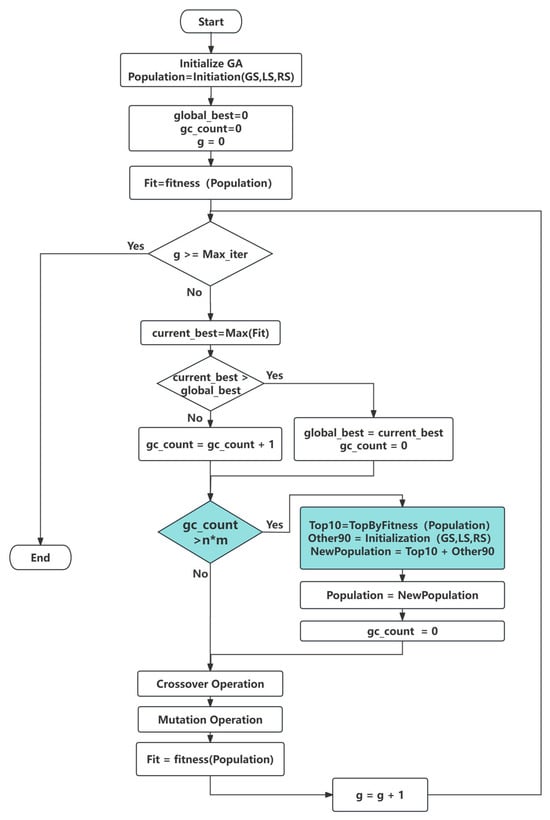
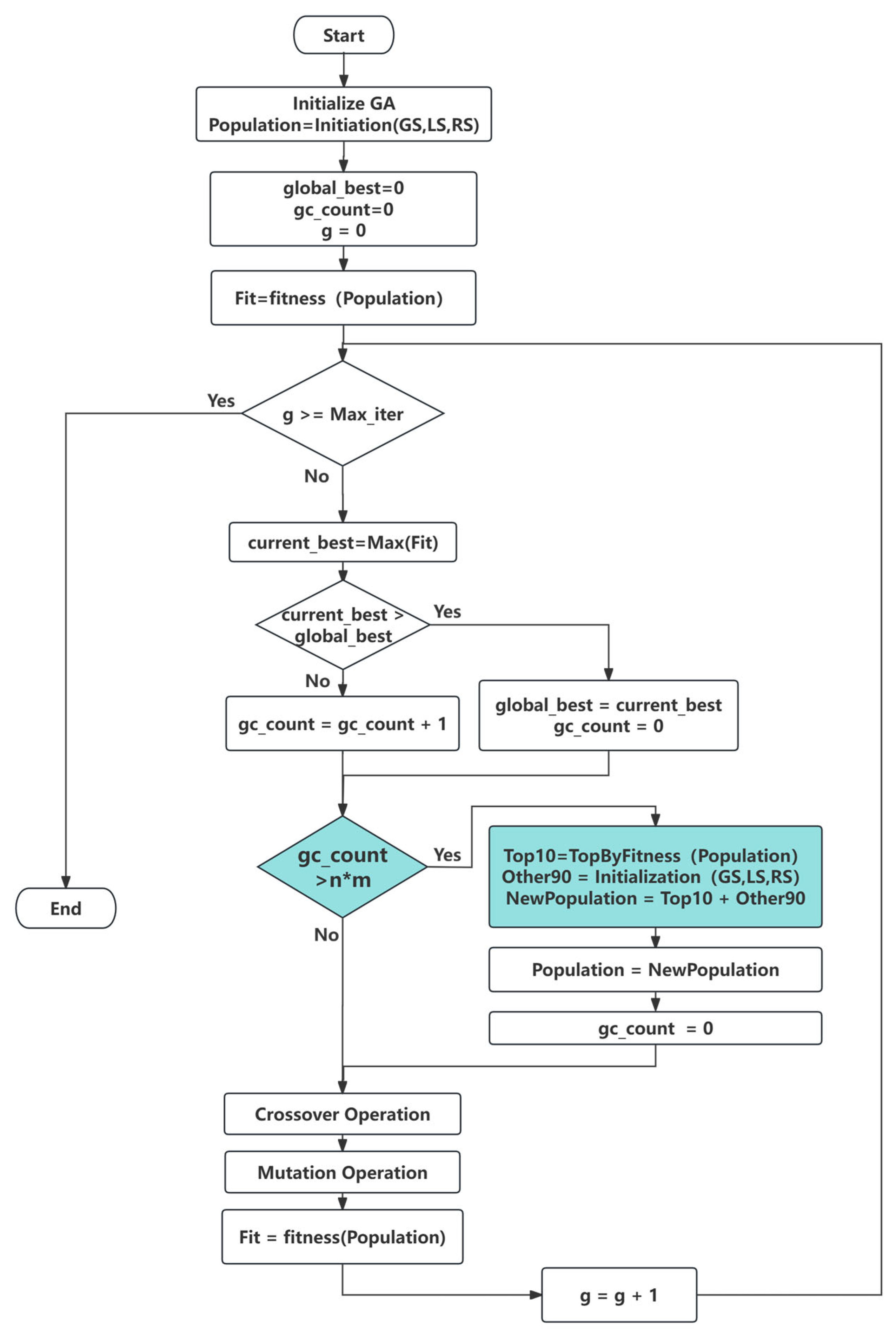
To enhance the algorithm’s capability to escape local optima, a population restructuring mechanism is proposed. When stagnation at a local optimum is detected, the algorithm evaluates the neighboring solutions of each individual and dynamically adjusts the population structure based on their fitness, thereby redirecting the search toward more promising regions of the solution space. Specifically, the top 10% of chromosomes with the highest fitness are preserved, while the remaining 90% are reinitialized to recommence the search process. This approach not only strengthens solution space exploration but also effectively mitigates premature convergence, leading to improved final solutions.

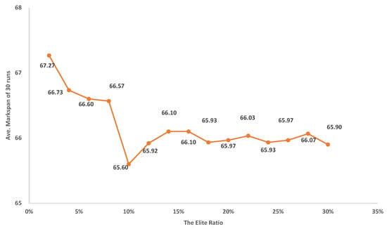
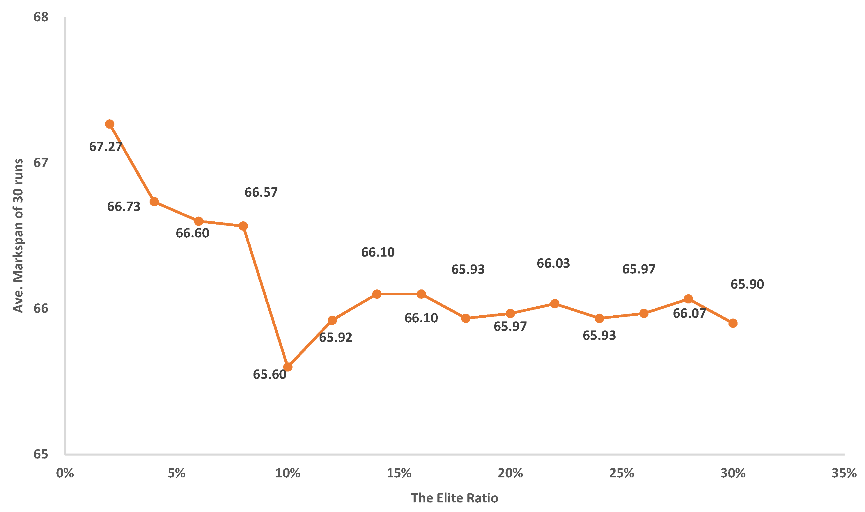
As shown in the Figure 1, the elite proportion of 10% yields the optimal average makespan—the key evaluation metric in this study. Notably, this specific proportion represents a novel configuration introduced, as it has not been explicitly recommended or systematically validated in prior literature on elite retention strategies.

Figure 1. Sensitivity Analysis on Elito Ratio.

When the elite proportion is reduced below 10% (e.g., 5%), the algorithm exhibits insufficient exploitation of high-quality solutions due to an inadequate number of elite chromosomes guiding the search. This leads to slower convergence and an increased tendency to become trapped in local optima. Conversely, when the proportion exceeds 10% (e.g., 15–30%), performance declines as excessive elitism reduces population diversity. The resulting homogeneity weakens the algorithm’s ability to explore new regions of the solution space, often causing premature convergence.

Thus, the 10% elite proportion—introduced as an innovation in SSDA strategy—is empirically demonstrated to strike an optimal balance between exploration and exploitation. The sensitivity analysis conducted on the MK04 instance robustly supports this finding. To enhance the clarity and reproducibility of our method, this sensitivity analysis has been incorporated into the revised manuscript, providing a transparent and justified rationale for this parameter choice.

The highlight area of Figure 2 illustrates the detailed procedure.

Figure 2. Flowchart of the SSDA.

3.3. GA Parameter Adjustment Strategy Based on Multi-Q-Table Reinforcement Learning

Genetic algorithms require careful tuning of key parameters—especially crossover rate (P_c) and mutation rate (P_m) to balance exploration and exploitation. Poor tuning can either disrupt good solutions or limit new solutions. To address this, reinforcement a learning (RL) framework for dynamic parameter adaptation is proposed. RL is an adaptive optimization method [29] where an agent interacts with its environment [30] to learn a policy that maximizes cumulative reward.

RL framework adjusts three parameters in real time: P_c, P_m, and a new probability coefficient Pf for the QBMF operator. Unlike offline tuning tools (e.g., IRACE, ParamILS), RL enables dynamic adaptation during the search process. The agent continuously updates parameters based on runtime feedback (e.g., makespan improvement), responding to changes such as convergence slowdown or loss of diversity. This provides more flexible and context-aware control than static tuning.

Therefore, this study designs an Improved GA based on Reinforcement Learning (IGARL). The IGARL agent adjusts P_f, P_c, and P_m using both current and historical population states. This online adaptation removes the need for instance-specific training, improving generality across FJSP benchmarks.

To optimize multiple parameters simultaneously, we use multiple Q-tables [31] that share the same state space but have separate action and reward dimensions for each parameter.

The iterative formula for Q-learning in reinforcement learning [32,33] is as follows:

$$Q(s_t,a_t)=(1-\alpha )Q(s_t,a_t)+\alpha [r_{t+1}+\gamma maxQ(s_{t+1},a_{t+1}\left)\right]$$

(2)

The iterative formula for the SARSA algorithm [30,34] is as follows:

$$Q(s_t,a_t)=(1-\alpha )Q(s_t,a_t)+\alpha [{\mathrm{r}}_{t+1}+\gamma Q(s_{t+1},a_{t+1}\left)\right]$$

(3)

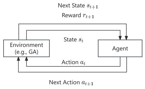
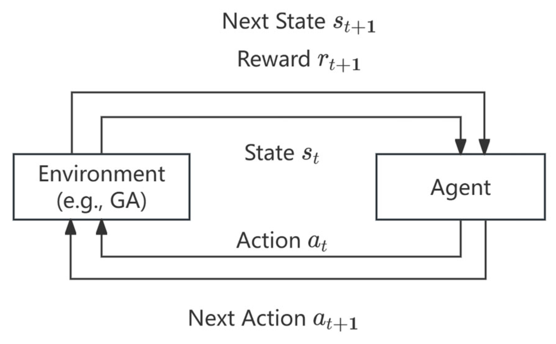
In Equations (2) and (3), α represents the learning rate, r_t+1 is the reward received after taking an action in state s_t, and γ refers to the discount factor. Here, the population within the genetic algorithm is treated as the agent [35], with the primary goal being parameter optimization. The configurations of states, actions, and rewards within the reinforcement learning framework are depicted in Figure 3.

Figure 3. Reinforce the learning block diagram.

3.3.1. State Set

In FJSP, the makespan defines the fitness of the chromosomes. Consequently, the environment construction in IGARL takes into account three key factors: the average fitness of the population, the fitness of the best-performing chromosome, and the fitness variance. These factors are normalized by comparing them to their respective values in the initial population.

The average fitness of the population, represented as f^∗, indicates the overall performance level of the population. A high average fitness value signifies that individuals generally perform well, whereas a low average fitness value implies weaker performance. The population size is denoted by N, and the calculation method is outlined in Equation (4).

$$f^{*}={\displaystyle \frac{\sum _{i=1}^{N}f\left(x_i^t\right)}{\sum _{i=1}^{N}f\left(x_i^1\right)}}$$

(4)

The optimal fitness of the population, represented as m^∗, indicates the highest performance level achieved by the best individual within the population. The calculation method is provided in Equation (5).

$$m^{*}={\displaystyle \frac{\mathrm{m}\mathrm{a}\mathrm{x}\left[f\right(x_i^t\left)\right]}{\mathrm{m}\mathrm{a}\mathrm{x}\left[f\right(x_i^1\left)\right]}}$$

(5)

Population diversity, denoted as d^∗, quantifies the variation among individuals within the population. Higher diversity indicates a wider spread of individuals across the solution space, enhancing the algorithm’s exploratory capabilities. On the other hand, lower diversity increases the likelihood of the algorithm becoming stuck in a local optimum. Variance is commonly employed to measure population diversity, with its calculation outlined in Equation (6).

$$d^{*}={\displaystyle \frac{\sum _{i=1}^N\left|f(x_i^t)-\frac{\sum _{i=1}^{N}f(x_i^t)}{N}\right|}{\sum _{i=1}^N\left|f(x_j^1)-\frac{\sum _{j=1}^{N}f(x_j^1)}{N}\right|}}$$

(6)

$$S^{*}=w_1{f}^{*}+w_2{d}^{*}+w_3{m}^{*}$$

(7)

In the Equation, f(x^t) denotes the fitness value of the chromosomes in generation t of the population, f(x¹) represents the fitness value of the chromosomes in the first generation, and max[f(x^t)] indicates the fitness value of the best-performing chromosome in the generation t.

Equations (4)–(6) denote the normalized average fitness, the fitness of the optimal chromosome, and the variance of the fitness of the population, respectively, as calculated from the first generation. Equation (7) defines the population state value, where the w₁, w₂, and w₃ are assigned respectively.

Based on the methodology outlined in [36], we conducted a series of experiments to determine the optimal weight combination for the parameters. The experimental results is summarized in the Table 5, demonstrate that the weight set w₁ = 0.2, w₂ = 0.6, and w₃ = 0.2 yields the best performance in terms of the average makespan.

Table 5. Performance comparison of makespan under different weight combinations.

#	Parameter Setting	Min (Makespan)	Max (Makespan)	Ave.
1	w1 = 0.2, w2 = 0.6, w3 = 0.2	63	67	65.6
2	w1 = 0.6, w2 = 0.2, w3 = 0.2	64	67	66.1
3	w1 = 0.2, w2 = 0.2, w3 = 0.6	63	67	65.7
4	w1 = 0.4, w2 = 0.4, w3 = 0.2	63	69	67.2
5	w1 = 0.4, w2 = 0.2, w3 = 0.4	63	68	66.2
6	w1 = 0.2, w2 = 0.4, w3 = 0.4	64	68	66.2
7	w1 = 0.35, w2 = 0.35, w3 = 0.3	64	68	66.1

The experiments, conducted with the condition of a population size of 480 and a maximum of 720 iterations, were executed 10 times using different random seeds on MK06 instance.

As shown in the Table 5, the weight combination w₁ = 0.2, w₂ = 0.6, and w₃ = 0.2 achieves the lowest average makespan of 65.6, outperforming all other tested configurations. This result confirms that this specific weight assignment optimally balances the contributions of the three components in our model, leading to the most efficient scheduling performance. Therefore, we adopt w₁ = 0.2, w₂ = 0.6, and w₃ = 0.2 as the final parameter setting for the proposed method.

The number of states is momentous. Too many states could be more precisely for self-learning, but it needs more exploration, which will affect the convergence of GA, while too few states could lead to poor results. According to the fitness of GA for solving FJSP and the value of S*, the state set is divided into 20 states for S = [s(1), s(2), …, s(19), s(20)] [36], where the interval value of S* is set as 0.05, e.g., when S* ∈ [0, 0.05], s = s(1); S* ∈ [0.05, 0.10], s = s(2) and so on.

The comprehensive sensitivity experiments are conducted and the results are shown in Table 6. The results clearly show that when the number of discrete states deviates from 20, the performance metrics such as Min, Max, and average values deteriorate. For example, with 10 discrete states, the average value is 68.3; with 40 discrete states, it is 67.4. In contrast, when using 20 discrete states, the average value reaches 67.0, which is relatively optimal. These experimental findings strongly support our design choice of using 20 discrete states, indicating that it is not an arbitrary decision but is based on solid experimental evidence.

Table 6. Discrete state of state’s sensitivity experiment.

#	Discrete State	Min (Makespan)	Max (Makespan)	Ave.	SD
1	10	64	70	68.3	1.83
2	20	63	67	67.0	1.94
3	30	64	67.4	67.4	1.51

Test conditions: Based on the MK06 case, tests were conducted with a population size of 500 and 200 iterations. The state discretization levels of 10, 20, and 40 were each tested 10 times, and the results were statistically analyzed.

3.3.2. Action Set

The agent adjusts the genetic algorithm by taking different actions for each generation of the population to improve the queen bee mating probability (P_f), the crossover probability (P_c), and the mutation probability (P_m). The calculation logic for P_c, P_m, and P_f is the same. P_c’s formula is provided in Equation (8) as an example.

$$p_c(t)=p_c(t-1)+\Delta {\omega }_1, \Delta {\omega }_1=\left\{\begin{array}{l}-0.02\\ 0.00\\ +0.02\end{array}\right.$$

(8)

The formula describes how the variable P_c evolves over time. The actions include three types: increase, remain unchanged, and decrease. At each time step t, its value is updated by adding a specific increment $\Delta {\omega }_1$ to its value from the previous time step t − 1. The increment $\Delta {\omega }_1$ can be either −0.02, 0.00, or +0.02, depending on performance. If performance improves then add 0.02 to the relevant parameters, and when it gets worse then subtract 0.02.

The sensitivity experiment has been conducted to further verify the settings and the result is shown in Table 7. Based on the experimental results for instance mk06, the configuration with 10 discrete states achieves the best overall performance. It yields the lowest minimum makespan (63), the lowest average makespan (66.9), and maintains a competitive standard deviation (1.97). While the setting with 5 discrete states shows a slightly lower average (67.0), its higher variability (SD = 1.94) and worse minimum makespan (64) make it less robust. The configuration with 20 discrete states performs the worst across all metrics. Therefore, 10 discrete states provides the optimal balance between solution quality and stability for this instance.

Table 7. Discrete state of action’s sensitivity experiment.

#	Discrete State	Min (Makespan)	Max (Makespan)	Ave.	SD
1	5	64	69	67.0	1.94
2	10	63	69	66.9	1.97
3	20	66	70	67.9	1.29

In the improved genetic algorithm, the queen bee mating probability (P_f) is initially set using heuristic methods, where simple experiments helped determine a relatively reasonable range of P_f ∈ [0.8, 1.0]. Reinforcement learning is then utilized to dynamically adjust this parameter. Additionally, a higher crossover probability (P_c) typically promotes genetic exchange among individuals in the population, increasing the likelihood of generating better solutions. This enhances the algorithm’s global search capability, allowing faster exploration of different regions in the solution space and avoiding premature convergence to local optima. In this study, the crossover probability is set within a relatively high range of P_c ∈ [0.8, 1.0].

On the other hand, appropriate mutation operations help maintain population diversity, preventing the population from losing diversity prematurely and leading to premature convergence. However, the mutation probability (P_m) should not be excessively high, as this would make the algorithm approximate a random search, negatively affecting efficiency and performance. In this study, the value of P_m is set within the range [0.1, 0.3].

The adjustment width for all three parameters is set to 0.2. The action set size is 10, with each parameter adjustment taking values of −0.02, 0 and +0.02.

3.3.3. Reward Mechanism

The reward mechanism offers feedback on the immediate impact of taking a specific action within a given state. The reward for the agent is calculated based on the changes in the average fitness of the population and the fitness of the best-performing chromosome. The learning objective is to optimize the parameters P_c, P_m and P_f with the corresponding rewards R_c, R_m, and R_f fed back to the environment. The specific calculation formulas are as follows:

$$R_c={\displaystyle \frac{\mathrm{m}\mathrm{a}\mathrm{x}\left[f\right(x_i^t\left)\right]-max\left[f\right(x_i^{t-1}\left)\right]}{\mathrm{m}\mathrm{a}\mathrm{x}\left[f\right(x_i^{t-1}\left)\right]}}$$

(9)

If the adjusted P_c leads to the optimal individual’s fitness surpassing that of the previous generation, it is deemed an effective exploration action, and the agent receives a reward. Equation (9) provides the reward for the adjusted P_c.

$$R_m={\displaystyle \frac{\sum _{i=1}^{N}f\left(x_i^t\right)-\sum _{i=1}^{N}f\left(x_i^{t-1}\right)}{\sum _{i=1}^{N}f\left(x_i^{t-1}\right)}}$$

(10)

Likewise, if adjusting P_m enhances the population’s average fitness, the agent is rewarded. The reward for the adjusted P_m is represented by Equation (10).

$$R_{\mathrm{f}}={\displaystyle \frac{\mathrm{m}\mathrm{a}\mathrm{x}\left[f\right(x_i^t\left)\right]-max\left[f\right(x_i^{t-1}\left)\right]}{\mathrm{m}\mathrm{a}\mathrm{x}\left[f\right(x_i^{t-1}\left)\right]}}$$

(11)

For the adjustment of P_f, considering that both the preset values of P_c and P_f are relatively high [0.8, 1.0], the agent’s reward is also determined based on changes in the fitness of the population’s optimal chromosome. Equation (11) provides the reward for the adjusted P_f.

3.4. IGARL Model Architecture

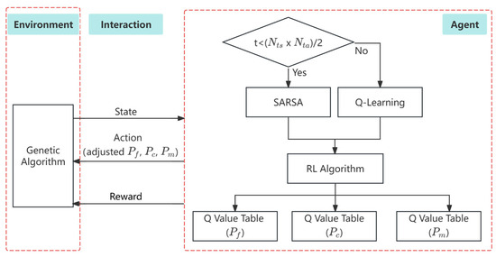
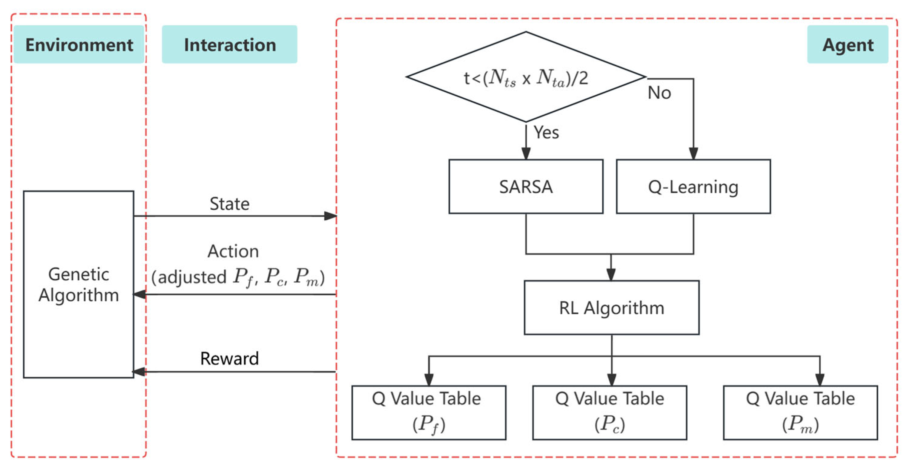
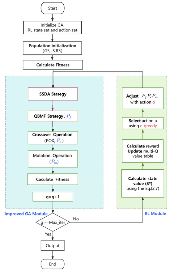
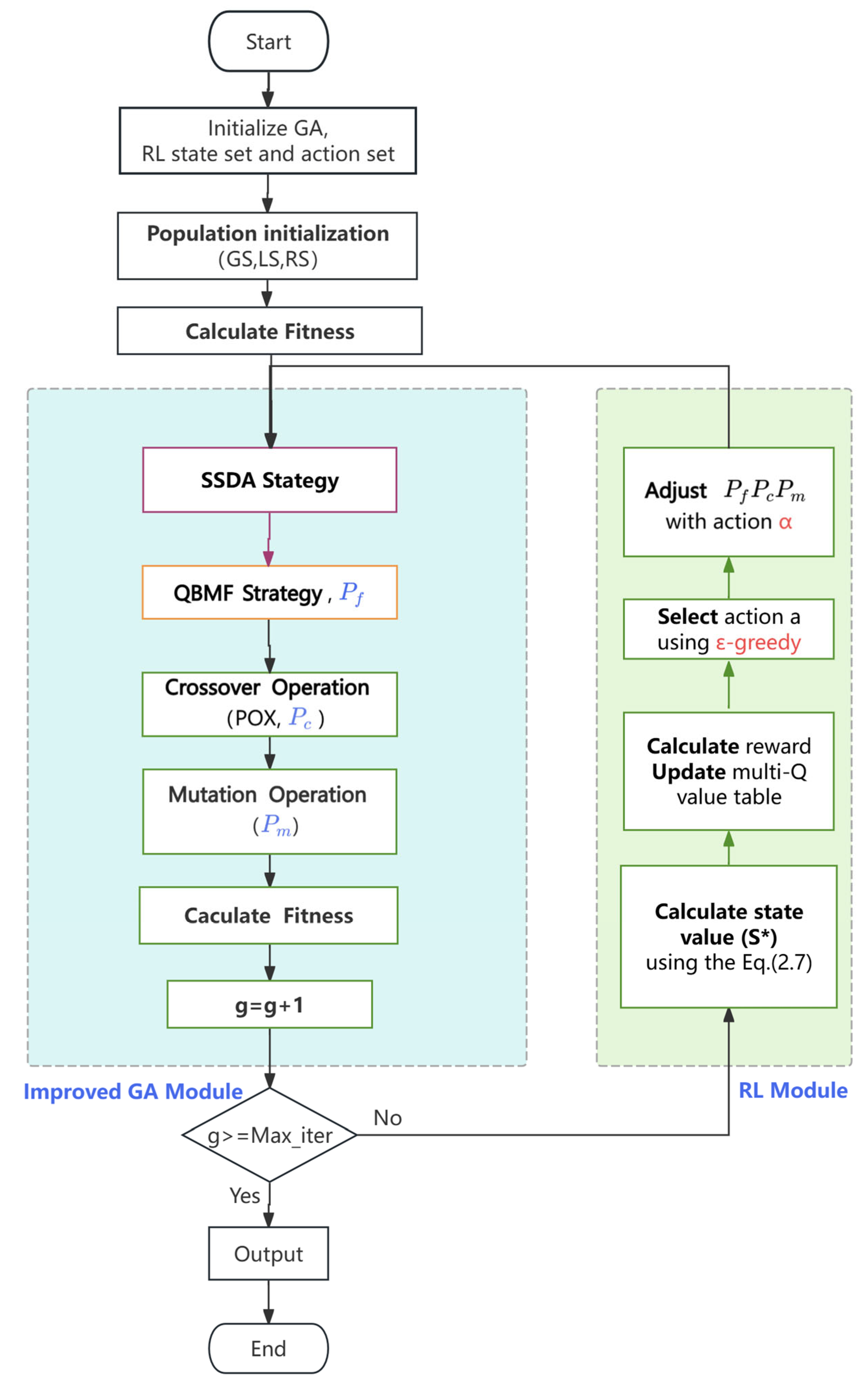
The combination of GA and RL demonstrates the advantages of “global exploration + local optimization,” making it suitable for tasks requiring a balance between breadth and depth of search, as well as handling dynamic and complex environments. The integration of these two approaches significantly enhances algorithm robustness, adaptability, and solution quality, especially in hybrid frameworks such as GA-RL [37]. The combined model of genetic algorithms and reinforcement learning consists of three components: environment, learning module, and reinforcement process. In this framework, the genetic algorithm is treated as the environment, where each iteration transitions the state from st to st+1. The learning module comprises a reinforcement learning agent and a Q-value table, where the agent represents the virtual object in the reinforcement learning algorithm. SARSA and Q-learning [23] are employed as key components of the learning module, leveraging their respective advantages to accelerate learning and improve overall performance. This approach applies SARSA and Q-learning at different stages. During the initial phase of reinforcement learning and GA, the SARSA algorithm is combined with the genetic algorithm to form IGARL. Once specific conditions are met, the SARSA algorithm transitions to the Q-learning algorithm. The conversion condition [36] guarantees Q-learning algorithms have adequate learning materials or learning experiences, which is determined by the quantity of Non-zero Q value, and the quantity of Q value is relevant to the number of states and the number of actions. So, in IGARL, the conversion condition is considered in the decision box of Figure 4.

Figure 4. Operational framework of IGARL.

The operational framework of IGARL is depicted in Figure 4. In the RL model, a hybrid strategy proposed by [30] is adopted, integrating SARSA and Q-learning for Q-table updates. Here, t represents the current iteration, N_ts denotes the total number of states, and N_ta denotes the total number of actions. The collaborative mechanism for the hybrid strategy is as follows: If the iteration count t is less than half the product of N_ts and N_ta, the Q-table is updated using the SARSA strategy. Otherwise, when t is greater than or equal to half the product of N_ts and N_ta, the Q-learning strategy is applied for Q-table updates.

The SARSA algorithm will be converted to the Q-learning algorithm if the conversion condition is met. This mechanism enables SARSA and Q-learning to collaboratively update the same Q-table, complementing each other’s strengths and improving the efficiency of Q-table optimization. Additionally, due to the dynamic adjustment of three parameters in the GA—P_f, P_c, and P_m, three separate Q-tables are used to record intermediate states, preventing mutual interference.

3.5. IGARL Algorithm Workflow

To address the slow convergence speed, susceptibility to local optima, and reliance on fixed mutation and crossover rates in genetic algorithms for the FJSP Problem, a scheduling optimization method based on collaborative agent reinforcement learning is proposed. This algorithm incorporates the QBMF to improve convergence speed and introduces a solution space diversity awakening strategy to avoid local optima. Through reinforcement learning, the algorithm can intelligently adjust key parameters, such as population selection rate, genetic crossover probability, and mutation probability. It evaluates state values comprehensively from three dimensions: population average fitness, optimal fitness, and population diversity. The complete procedure is outlined in below Algorithm 2, and Figure 5 illustrates the IGARL algorithm’s flowchart.

Algorithm 2: IGARL Algorithm Workflow

1:    begin

2:    population = GLR_Hybrid_Initialization(population_size)

3:    Initialize Q_table with all zeros

4:    iteration = 0

5:    best_solution = NULL

6:    previous_state = NULL

7:    previous_action = NULL

8:            while iteration < max_iterations do

9:                    for each chromosome in population do

10:                              chromosome.fitness = Evaluate_Fitness(chromosome)

11:                          end for

12:                  if Tunnel_Vision_Detected(population) then

13:                          population = Diversity_Awakening_Strategy(population)

14:                      end if

15:                      selected_population = Tournament_Selection(population, QBMF_Strategy)

16:                      offspring_population = Crossover(selected_population, crossover_rate)

17:                      offspring_population = Mutation(offspring_population, mutation_rate)

18:                      for each chromosome in offspring_population do

19:                            chromosome.fitness = Evaluate_Fitness(chromosome)

20:                      end for

21:                      current_best = Find_Best_Chromosome(offspring_population)

22:                      if best_solution is NULL or current_best.fitness > best_solution.fitness then

23:                          best_solution = current_best

24:                      end if

25:                      iteration = iteration + 1

26:                      if iteration >= max_iterations then

27:                          Break

28:                      end if

29:                      avg_fitness = Calculate_Average_Fitness(offspring_population)

30:                      best_fitness = current_best.fitness

31:                      population_diversity = Calculate_Diversity(offspring_population)

32:                      current_state = (avg_fitness, best_fitness, population_diversity)

33:                      reward = Calculate_Reward(avg_fitness, best_fitness, population_diversity)

34:                      if previous_state is not NULL then

35:                            old_q_value = Q_table[previous_state][previous_action]

36:                            max_future_q = MAX(Q_table[current_state][])

37:                            new_q_value = old_q_value + learning_rate_alpha * (reward + discount_factor_gamma * max_future_q − old_q_value)

38:                            Q_table[previous_state][previous_action] = new_q_value

39:                      end if

40:                      action = Greedy_Action_Selection(Q_table, current_state)

41:                      queen_mating_prob, crossover_rate, mutation_rate = Adjust_Parameters(action)

42:                      previous_state = current_state

43:                      previous_action = action

44:                      population = offspring_population

45:          end while

46:  return best_solution

Figure 5. The IGARL algorithm flowchart.

4. Experimental Analysis

The experiments were carried out on a laptop running in windows server 2019 and Python 3.12 with parameters following the original literature. Simulations ran on a server with an Intel Xeon Gold 5218 CPU (2.30 GHz), 64 GB RAM.

4.1. Analysis of Algorithm Improvement Effects

4.1.1. Effects of Queen Bee Mating Flight Strategy

In this study, the standard Brandimarte benchmark instances in the field of genetic algorithms were selected as experimental subjects. These instances were utilized to assess the algorithm’s performance and generate experimental results. The basic GA represents the initial state of the algorithm studied in this paper. The QBMF draws inspiration from the active selection mechanism in queen bee mating behavior. By dynamically adjusting resource allocation rules, this strategy enhances the optimization efficiency of the algorithm and accelerates its convergence speed. After applying the QBMF, rapid optimization was effectively achieved, and the number of iterations required to reach the optimal solution was significantly reduced.

The experimental results show that the algorithm employing the QBMF exhibits significantly better convergence performance compared to the basic GA. Among the 10 benchmark instances, 8 instances achieved the same optimal solution (C_max) as the basic GA, while the number of iterations decreased significantly and was consistently lower than that of the basic GA. The convergence speed improvement (CSI) increased by 10–60%. Furthermore, the strategy demonstrated substantial convergence speed improvements across different population sizes. The formula for calculating CSI is shown in Equation (12), and the detailed results are presented in Table 8.

CSI = (C_max − C_max*)/C_max × 100%

(12)

Table 8. Data Comparison Between GA with QBMF and Basic GA.

Instance	n × m	BKS	GA		GA (QBMF) *			GA (QBMF)
			Cmax	Tmin	C = Cmax *	Tmin *	CSI (%)	Cmax **	Tmin **
MK01	10 × 6	36	42	9	42	6	33%	42	6
MK02	10 × 6	24	29	31	29	28	10%	28	87
MK03	15 × 8	204	204	19	204	13	32%	204	13
MK04	15 × 8	48	66	90	66	36	60%	65	81
MK05	15 × 4	168	176	54	176	24	56%	173	40
MK06	10 × 10	33	73	99	73	68	31%	73	68
MK07	20 × 5	133	145	68	150	23	/	150	23
MK08	20 × 10	523	523	20	523	11	45%	523	11
MK09	20 × 10	299	317	108	317	57	47%	310	111
MK10	20 × 15	165	225	226	229	198	/	229	198

*: The Number of Iterations reach the Basic GA’s Optimal Solution After applying QBMF. **: The final result of improved GA with QBMF.

In the QBMF, the optimal chromosome from the previous iteration (the queen bee) undergoes crossover or mutation operations with 15 other chromosomes. This process allows the superior genes of the queen bee to be more effectively passed on to the next generation, thereby improving the overall fitness of the population and achieving rapid convergence. Additionally, under the QBMF, the optimal solutions of 8 out of 10 benchmark instances are superior to those obtained with the basic GA. These results indicate that the QBMF significantly enhances both convergence speed and the quality of the optimal solutions.

A statistical significance test was conducted to compare the results of the GA enhanced with QBMF and the standard GA. The test yielded a statistic of 7.0 with a p-value of 0.035. This result indicates that the performance improvement achieved by the QBMF enhanced GA is statistically significant, thereby demonstrating the robustness and stability of the improved outcomes.

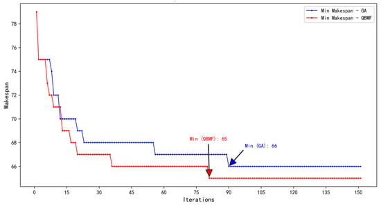
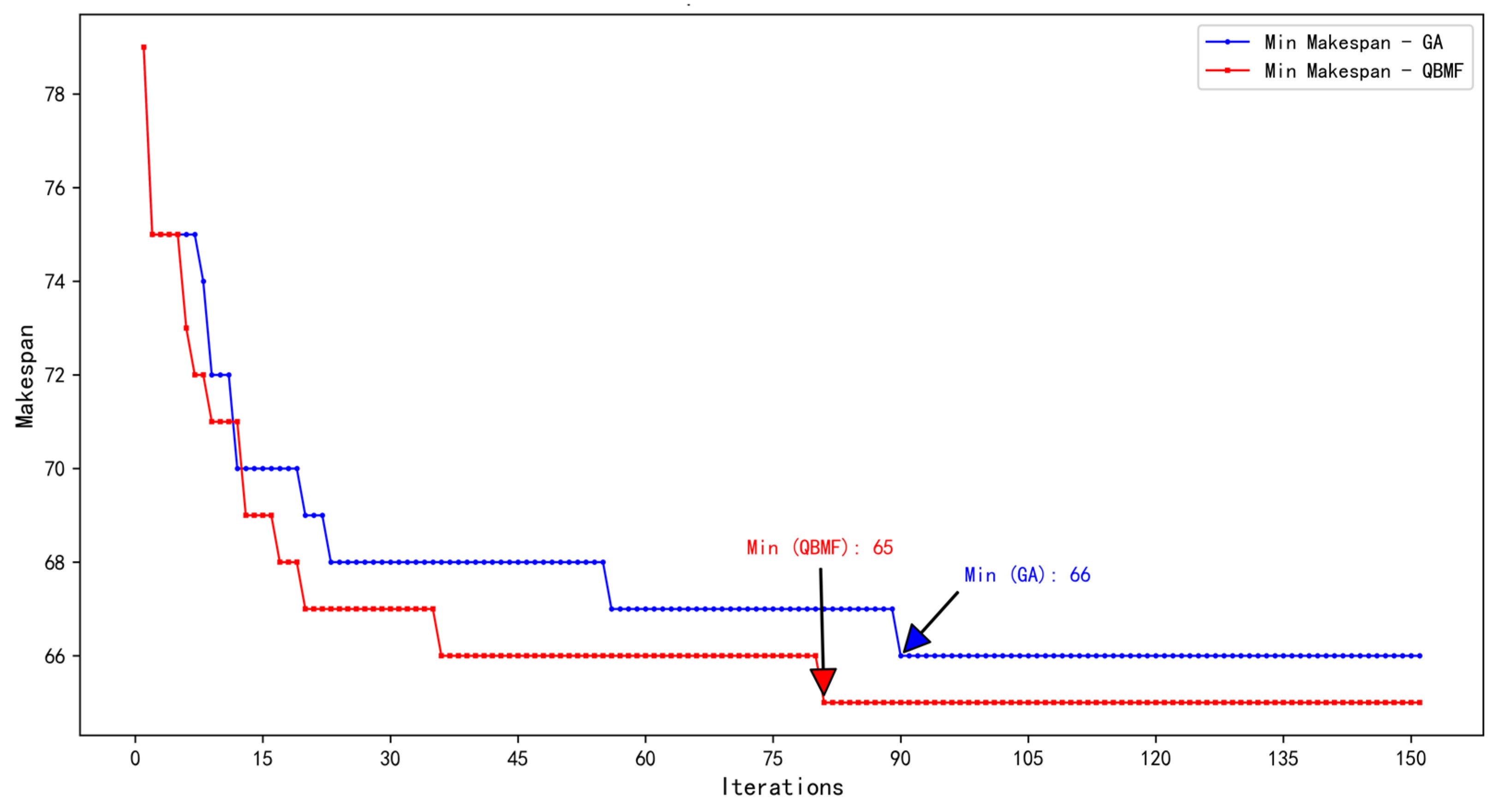
The implementation effects of the QBMF are illustrated in Gantt charts, as shown in Figure 6 and Figure 7 (using MK04 and MK05 as examples). Taking the standard instance MK04 as an example, as depicted in Figure 6, the basic GA requires 90 iterations to achieve the optimal solution of 66. In contrast, the improved genetic algorithm with the QBMF requires only 36 iterations to reach the same optimal solution, resulting in a 60% improvement in convergence speed. Additionally, the quality of the optimal solution demonstrates superior performance.

Figure 6. Implementation Effects of the QBMF (MK04).

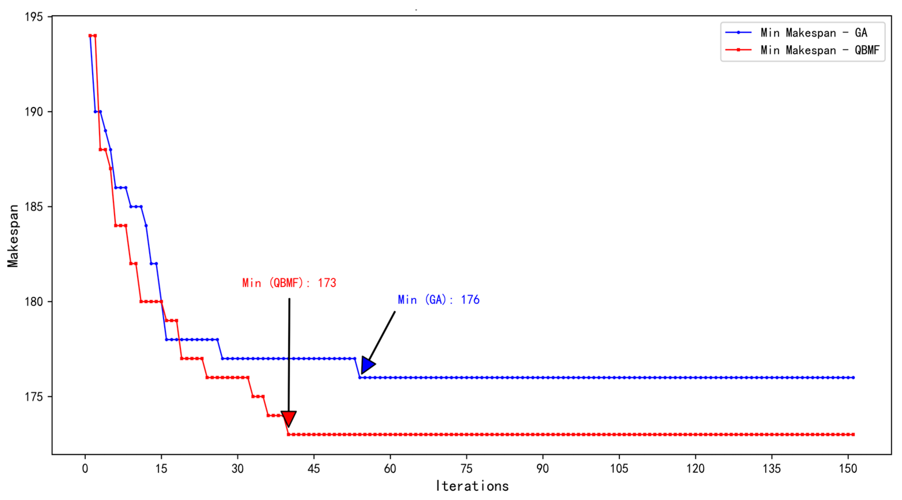
Figure 7. Implementation Effects of the QBMF (MK05).

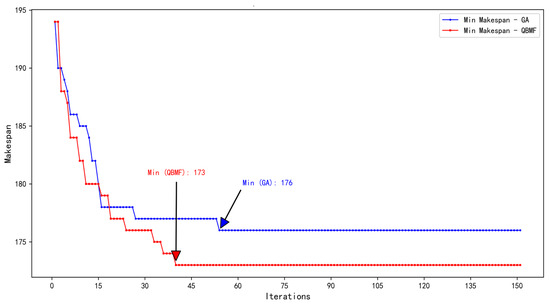
Similarly, in the standard instance MK05, as illustrated in Figure 7, comparable experimental results were observed. The basic GA requires 54 iterations to achieve the optimal solution of 176. In contrast, the improved genetic algorithm with the QBMF requires only 24 iterations to reach the same solution, resulting in a 56% improvement in convergence speed. Furthermore, the quality of the optimal solution is enhanced, improving from 176 to 173.

4.1.2. Effect of the Solution Space Diversity Awakening Strategy

The adoption of the QBMF in genetic algorithms (GAs) significantly enhances convergence performance. However, in two test cases, no new optimal solutions were generated after GC ($\mathrm{n}\ast \mathrm{m}$) consecutive iterations. Based on the tunnel vision phenomenon judgment rule, this situation was identified as a local optimum. To prevent getting stuck in local optima, an improved strategy was developed by combining the QBMF with a solution space diversity awakening mechanism. This strategy retains the top 10% of chromosomes with the best fitness and reinitializes the remaining chromosomes, restarting the algorithm to explore a broader solution space and escape local optima.

The combined effects of the QBMF and the SSDA are shown in Table 9. Experiments were conducted using three different algorithms: the basic GA, the GA with the QBMF, and the GA with both the QBMF and the SSDA. To ensure consistency, the same random seed was used for initialization, guaranteeing that the population at the start of each algorithm was identical. In these experiments, T_min represents the number of iterations required to achieve the optimal solution C_max.

Table 9. Result between the improved genetic algorithm (QBMF + SSDA) and basic GA.

Instance	n × m	BKS	GA		GA (QBMF + SSDA)
			Cmax	Tmin	Cmax	Tmin	Mean (Cmax)	SD (Cmax)
MK01	10 × 6	36	42	9	42	6	42.00	0.00
MK02	10 × 6	24	29	31	28	87	28.20	0.55
MK03	15 × 8	204	204	19	204	13	204.00	0.00
MK04	15 × 8	48	66	90	65	81	65.57	1.37
MK05	15 × 4	168	176	54	173	40	173.80	0.89
MK06	10 × 10	33	73	99	72	107	70.40	1.73
MK07	20 × 5	133	145	68	144	189	145.63	1.27
MK08	20 × 10	523	523	20	523	11	523.00	0.00
MK09	20 × 10	299	317	108	309	280	310.43	1.14
MK10	20 × 15	165	225	226	224	210	232.43	3.96

When comparing the GA with the queen bee mating and diversity awakening strategies to the basic GA, improvements in the optimal solution C_max were observed in 8 out of 10 test cases, with the exceptions being MK03 (204) and MK08 (523), where the values remained unchanged. Notably, for large populations such as MK07 and MK10, which were previously stuck in local optima due to tunnel vision, the combined strategy successfully overcame local optima and achieved new optimal solutions. These results clearly demonstrate the effectiveness of integrating the QBMF with the solution space diversity awakening mechanism in genetic algorithms.

Mean (C_max) and SD (C_max) are calculated based on the average makespan and its standard deviation from 10 independent runs for each benchmark instance.

The standard deviation (SD) values presented in the table quantify the stability and robustness of the proposed GA (QBMF + SSDA) algorithm across multiple benchmark instances. Specifically, lower SD values indicate more consistent and reliable performance in obtaining makespan (C_max) results over repeated runs. For example, instances such as MK01, MK03, and MK08 achieved an SD of 0.00, demonstrating perfect reproducibility and convergence to the same optimal or near-optimal solution in every trial. In contrast, instances with higher SD values, such as MK10 (SD = 3.96) and MK06 (SD = 1.73), reflect greater variability in outcomes, which may be attributed to the increased complexity of these problem instances. Overall, the consistently low SD values across most instances confirm that the enhanced algorithm not only improves solution quality but also maintains high solution stability, a key indicator of its practical reliability.

4.2. Comparison Between IGARL and Other Algorithms

To validate the effectiveness of the proposed improved genetic algorithm, the Improved Genetic Algorithm based on Reinforcement Learning (IGARL) was implemented using PyCharm 2024.3.2. The MK01-MK10 dataset designed by Brandimarte was selected as the test benchmark. For comparability with the SLGA algorithm [36], the population size and maximum number of iterations were initialized as follows: the population size was set to $\mathrm{n}\ast \mathrm{m}\ast 5$ and the maximum number of iterations to $\mathrm{n}\ast \mathrm{m}\ast 10$. In the genetic algorithm, the initial probability of the QBMF (P_f) was set to 0.9, and the number of drones was set to 15, based on natural behavior. The initial crossover probability (P_c) was set to 0.85, and the initial mutation rate (P_m) to 0.24. Additionally, the learning factor (α) and discount rate (γ) for reinforcement learning were set to 0.75 and 0.2, respectively, as per the SLGA algorithm.

The effectiveness of IGARL for solving the FJSP problem was evaluated by comparing the optimal solutions generated by IGARL and those from various other algorithms on the MK01-MK10 benchmark instances. The comparisons included the following algorithms: the Self-Learning Genetic Algorithm (SLGA) proposed by [36], the Deep Reinforcement Learning Algorithm (AC-SD) proposed by [38], the Ensemble Reinforcement Learning Algorithm (D5QN) proposed by [39,40], the CNN-based Deep Reinforcement Learning Algorithm (PPO + CNN) proposed by [41], and the Genetic Algorithm with Improved Crossover Operators (IGA) proposed by [42]. The comparison results are presented in Table 10 and Figure 8.

Table 10. Data comparison between the IGARL algorithm and other algorithms.

Ins.	BKS	SLGA (2021)		AC-SD (2021)		D5QN (2023)		PPO + CNN (2024)		IGA (2024)		IGARL
		Cmax	RDP	Cmax	RDP	Cmax	RDP	Cmax	RDP	Cmax	RDP	Cmax	RDP
MK01	36	40	11.1	44	22.2	42	16.6	41	13.8	42	16.6	40	11.1
MK02	24	27	12.5	28	16.6	31	29.1	29	20.8	31	29.1	27	12.5
MK03	204	204	0.0	245	20.1	204	0.0	204	0.0	204	0.0	204	0.0
MK04	48	60	25.0	74	54.1	69	43.7	72	50.0	73	52.0	60	25.0
MK05	168	172	2.3	193	14.8	180	7.1	282	67.8	177	5.3	173	2.9
MK06	33	69	109.0	123	272.7	68	106.0	73	121.2	85	157.5	63	90.9
MK07	133	144	8.2	216	62.4	153	15.0	152	14.2	155	16.5	142	6.7
MK08	523	523	0.0	523	0.0	523	0.0	523	0.0	523	0.0	523	0.0
MK09	299	320	7.0	386	29.1	315	5.3	328	9.7	339	13.3	307	2.6
MK10	165	254	53.9	337	104.2	230	39.3	243	47.3	266	61.2	204	23.6
ARPD	-		22.9		59.6		26.2		34.5		35.2		17.5

Figure 8. Comparison of results between IGARL and other algorithms.

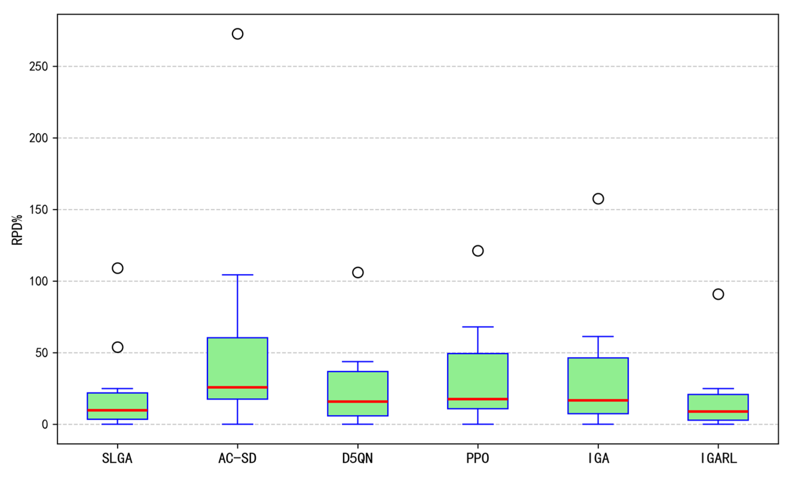
IGARL achieved better solutions than the other methods in 9 out of 10 standard test cases, demonstrating its superior solution quality. Additionally, the difference between the optimal solutions and the currently best known solutions, measured by the Relative Percentage Deviation (RPD) (see Equation (13)). The RPD, calculated against the Best-Known Solution (BKS), measures the relative percentage error of our algorithm’s solution and serves as our primary accuracy metric. The RPD of IGARL smaller than the other algorithms indicate its higher stability in individual cases. Further analysis of the average RPD across the 10 test cases showed that IGARL achieved an overall average RPD of 17.5%, compared to 22.9–59.6% for the other algorithms. This result highlights IGARL’s higher stability in both individual and overall test cases.

Moreover, a comparison of optimal solutions revealed that IGARL performed particularly well in solving more complex FJSP problems (e.g., MK09, MK10) with larger values of N and M, further demonstrating the feasibility and robustness of IGARL in FJSP optimization. For RPD calculations, BKS represents the current lower bound.

$$RPD={\displaystyle \frac{C_{\mathrm{m}\mathrm{a}\mathrm{x}}-BKS}{BKS}}\ast 100\%$$

(13)

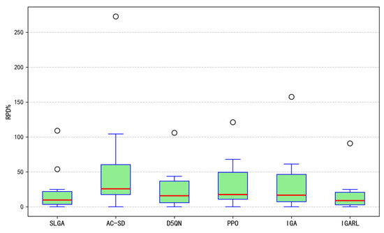
Figure 8 illustrates the overall distribution of RPD values. As shown in the Figure 8, the RPD values of IGARL are lower and more concentrated compared to other algorithms, indicating that IGARL outperforms its counterparts in solving the FJSP. This demonstrates that IGARL exhibits strong performance in addressing FJSPs, particularly for larger-scale problems, where it achieves superior results.

To further evaluate performance, the MK01-MK10 instances were independently executed 20 times. The optimal results obtained by the IGARL algorithm were compared with those of the SLGA algorithm. The comparative results are shown in Table 8.

As shown in Table 11, IGARL outperformed SLGA in most benchmark instances, except for MK03 and MK08 where both converged to identical solutions. This parity stems from the inherent low complexity and simple structure of these specific JSP instances. Their solution spaces lack challenging topography (e.g., numerous local optima or deceptive fitness landscapes), which fails to fully engage IGARL’s sophisticated adaptive exploration mechanisms. In such scenarios, even well-tuned conventional algorithms can efficiently approach optimal solutions, leaving minimal room for significant improvement by advanced hybrid methods. Therefore, the absence of performance gain on these instances does not indicate an IGARL limitation but underscores the context of problem difficulty. IGARL’s true advantage and robustness are more prominently manifested when applied to larger-scale, structurally complex instances like MK06, MK07, and MK10, where its adaptive capabilities are crucial for navigating intricate search spaces and achieving superior results. A comparison of the average optimal solutions from 20 runs (presented in Table 7) reveals that IGARL achieved an average optimal solution of 19.5% for each instance, significantly better than the SLGA algorithm’s average of 31.6%. These results highlight IGARL’s strong stability.

Table 11. A total of 20 times on the MK01-MK10 instances with IGARL and SLGA.

Instance	BKS	SLGA				IGARL
		Cmax	RDP	Cmax (Avg)	RDP (Avg)	Cmax	RDP	Cmax (Avg)	RDP (avg)
MK01	36	40	11.1	42	16.6	40	11.1	40.4	12.0
MK02	24	27	12.5	29.7	23.7	27	12.5	27.6	14.7
MK03	204	204	0.0	210.2	3.0	204	0.0	204	0.0
MK04	48	60	25.0	66.7	38.9	60	25.0	62.9	31.0
MK05	168	172	2.3	183.5	9.2	173	2.9	173.1	3.0
MK06	33	69	109.0	76.9	133.0	63	90.9	65.4	98.0
MK07	133	144	8.2	151.3	13.7	142	6.7	144.0	8.0
MK08	523	523	0.0	526.6	0.6	523	0.0	523	0.0
MK09	299	320	7.0	340.4	13.8	307	2.6	307.2	2.7
MK10	165	254	53.9	269.9	63.5	204	23.6	206.70	25.2
ARPD	-		22.9		31.6		17.5		19.5

The experimental results demonstrate that, compared to algorithms from existing literature, the proposed IGARL algorithm achieved superior solutions across multiple benchmark instances. Specifically, IGARL outperformed other algorithms, including the D5QN algorithm, PPO + CNN algorithm, AC-SD algorithm, IGA algorithm, and SLGA algorithm, in terms of solution efficiency, quality, and stability. Notably, IGARL maintained robust search performance even when solving larger-scale problems, showcasing its potential for addressing large-scale FJSP optimization.

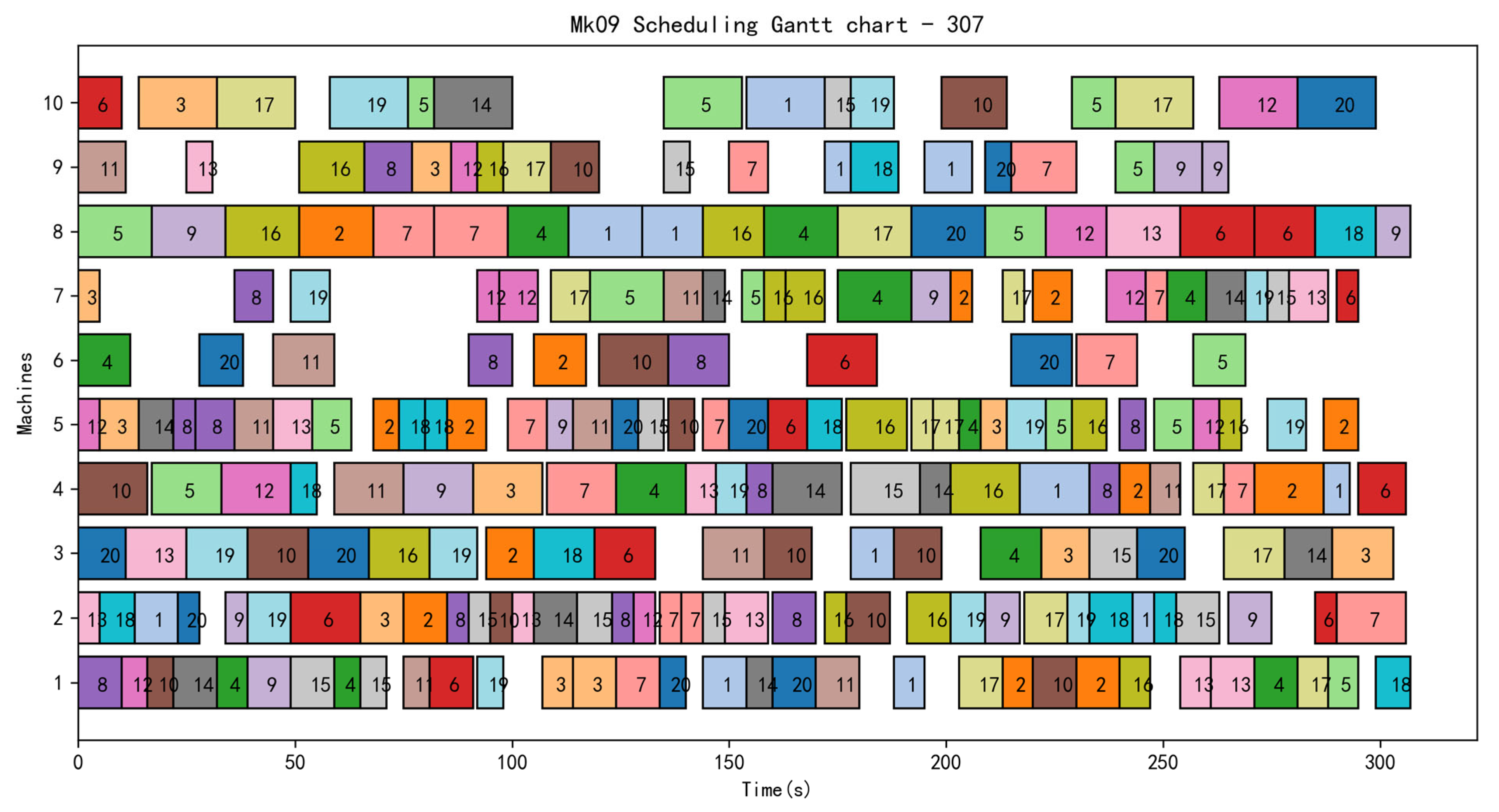
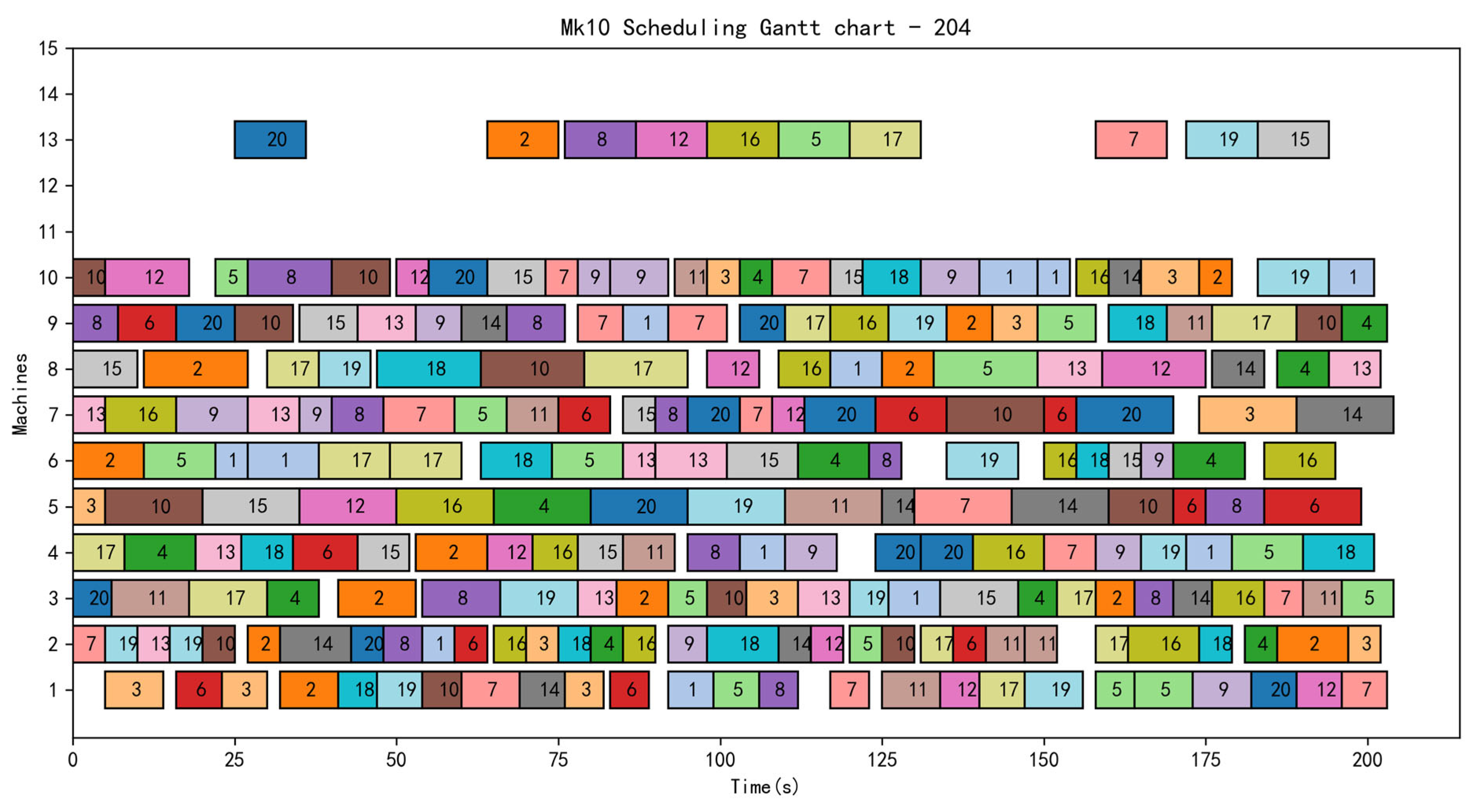
The Gantt chart for the IGARL-based MK09 instance (with C_max= 307) is presented in Figure 9, illustrating the optimal scheduling plan. In the chart, different colors represent distinct operations, while the sequence along the x-axis indicates the order of operations for each job. The duration of each block represents the operation’s processing time. The optimal scheduling time for this plan is 307. Similarly, the optimal scheduling time for the MK10 instance is 204, and the corresponding Gantt chart is presented in Figure 10.

Figure 9. The Gantt chart for the IGARL-based MK09 instance.

Figure 10. The Gantt chart for the IGARL-based MK10 instance.

To verify the performance of IGARL and evaluate the computational efficiency, we compared it with GA across standard benchmarks MK01–MK10, and the results are presented in Table 12. While IGARL incurs an average 6.27% increase in computation time compared to GA, this slight overhead is outweighed by its remarkable enhancements in solution quality, demonstrating a favorable trade-off between performance and efficiency.

Table 12. The running time of GA and IGARL based on instance.

Instance	n × m	GA (Sec.)	IGARL (Sec.)	Running Time Increase (%)
mk01	10 × 6	55.81	58.94	5.61
mk02	10 × 6	57.59	61.39	6.59
mk03	15 × 8	176.93	187.62	6.04
mk04	15 × 8	95.29	101.38	6.39
mk05	15 × 4	116.84	124.68	6.70
mk06	10 × 10	186.37	197.81	6.14
mk07	20 × 5	113.86	121.51	6.72
mk08	20 × 10	295.79	313.72	6.06
mk09	20 × 10	317.68	338.10	6.43
mk10	20 × 15	316.65	335.83	6.06
Ave.				6.27

Moreover, to further address concerns regarding scalability, we conducted additional experiments on larger-scale problems with 100 jobs and 50 machines. The results, shown in the attached file, indicate that even when faced with more complex scenarios, IGARL maintains its effectiveness. Although the computing time increases by 5.26% compared to GA in these larger instances, the consistent improvement in solution quality across different scales reinforces the practical value and robustness of our proposed method.

Experimental Conditions: Population size 100, maximum iterations 500. Under different random seeds, calculations were performed using the GA and IGARL algorithms, respectively. For each case from mk01 to mk10, 10 runs were conducted, recording the time consumption for each run, and the average time consumption across the 10 runs was taken.

5. Conclusions

In this study, an Improved Genetic Algorithm based on Reinforcement Learning (IGARL) is proposed to address the inherent challenges of traditional genetic algorithms in solving the Flexible Job-Shop Scheduling Problem (FJSP), such as slow convergence, vulnerability to local optima, and parameter sensitivity. The IGARL introduces several key innovations:

Optimization of Population Initialization and Selection: By integrating GS/LS/RS-based initialization and the Queen Bee Mating Flight (QBMF) strategy, the algorithm enhances the initial population quality and preserves superior genetic material. This approach not only optimizes the evolutionary trajectory but also significantly accelerates convergence.

Solution Space Diversity Awakening (SSDA) Strategy: To mitigate the risk of premature convergence and stagnation in local optima, a novel mechanism is designed to detect when the population is trapped and to selectively reset part of the population while retaining top individuals. This effectively maintains population diversity and enables the search to escape local optima.

Dynamic Parameter Adjustment via Reinforcement Learning: The use of reinforcement learning allows for real-time, adaptive adjustment of critical genetic parameters, such as crossover and mutation rates, as well as the queen bee mating probability, based on the evolving population state. This dynamic control enables the algorithm to better balance exploration and exploitation throughout the search process.

Experimental results on Brandimarte benchmark instances demonstrate that IGARL achieves a remarkable 10% to 60% improvement in convergence speed and consistently outperforms standard genetic algorithms in solution quality. Additionally, the algorithm shows strong stability, with the fluctuation of the average optimal solution remaining within 20%.

Despite these promising results, challenges remain, particularly regarding computational efficiency when addressing ultra-large-scale scheduling problems. Future research should focus on further optimizing the algorithm’s computational efficiency, investigating more advanced parameter self-adaptation strategies, and expanding the applicability of IGARL to more complex and diverse scheduling environments, such as dynamic or multi-objective production systems. Moreover, exploring hybrid approaches by integrating other machine learning techniques or leveraging parallel computing may further enhance the algorithm’s scalability and robustness.

References

- Gao, K.; Yang, F.; Zhou, M.; Pan, Q.; Suganthan, P.N. Flexible Job-Shop Rescheduling for New Job Insertion by Using Discrete Jaya Algorithm. IEEE Trans. Cybern. 2019, 49, 1944–1955. [Google Scholar] [CrossRef] [Scilit]
- Xu, Y.; Zhang, M.; Yang, M.; Wang, D. Hybrid quantum particle swarm optimization and variable neighborhood search for flexible job-shop scheduling problem. J. Manuf. Syst. 2024, 73, 334–348. [Google Scholar] [CrossRef] [Scilit]
- Azzouz, A.; Ennigrou, M.; Said, L.B. Flexible Job-shop Scheduling Problem with Sequence-dependent Setup Times using Genetic Algorithm. In Proceedings of the 18th International Conference on Enterprise Information Systems, Rome, Italy, 25–28 April 2016; pp. 47–53. [Google Scholar] [CrossRef] [Scilit]
- Jieran, Y.; Aimin, W.; Yan, G.; Xinyi, S. An Improved Grey Wolf Optimizer for Flexible Job-shop Scheduling Problem. In Proceedings of the 2020 IEEE 11th International Conference on Mechanical and Intelligent Manufacturing Technologies (ICMIMT), Cape Town, South Africa, 20–22 January 2020; pp. 213–217. [Google Scholar] [CrossRef] [Scilit]
- Jiang, X.; Tian, Z.; Liu, W.; Suo, Y.; Chen, K.; Xu, X.; Li, Z. Energy-efficient scheduling of flexible job shops with complex processes: A case study for the aerospace industry complex components in China. J. Ind. Inf. Integr. 2022, 27, 100293. [Google Scholar] [CrossRef] [Scilit]
- Zarrouk, R.; Bennour, I.E.; Jemai, A. A two-level particle swarm optimization algorithm for the flexible job shop scheduling problem. Swarm Intell. 2019, 13, 145–168. [Google Scholar] [CrossRef] [Scilit]
- Xu, M. Flexible job-shop scheduling optimization based on improved Gray Wolf algorithm. Front. Comput. Intell. Syst. 2024, 7, 25–28. [Google Scholar] [CrossRef] [Scilit]
- Luan, F.; Li, R.; Liu, S.Q.; Tang, B.; Li, S.; Masoud, M. An Improved Sparrow Search Algorithm for Solving the Energy-Saving Flexible Job Shop Scheduling Problem. Machines 2022, 10, 847. [Google Scholar] [CrossRef] [Scilit]
- Laha, D.; Gupta, J.N.D. An improved cuckoo search algorithm for scheduling jobs on identical parallel machines. Comput. Ind. Eng. 2018, 126, 348–360. [Google Scholar] [CrossRef] [Scilit]
- Fekih, A.; Hadda, H.; Kacem, I.; Hadj-Alouane, A.B. A hybrid genetic Tabu search algorithm for minimising total completion time in a flexible job-shop scheduling problem. Eur. J. Ind. Eng. 2020, 14, 763–781. [Google Scholar] [CrossRef] [Scilit]
- Alzaqebah, M.; Abdullah, S.; Malkawi, R.; Jawarneh, S. Self-adaptive bee colony optimisation algorithm for the flexible job-shop scheduling problem. Int. J. Oper. Res. 2021, 41, 53–70. [Google Scholar] [CrossRef] [Scilit]
- Wang, X.; Liu, C. A Hybrid Genetic Algorithm for Flexible Job Shop Scheduling Problem. In Proceedings of the 2022 5th World Conference on Mechanical Engineering and Intelligent Manufacturing (WCMEIM), Ma’anshan, China, 18–20 November 2022; pp. 1144–1148. [Google Scholar]
- Park, J.-S.; Ng, H.-Y.; Chua, T.-J.; Ng, Y.-T.; Kim, J.-W. Unified Genetic Algorithm Approach for Solving Flexible Job-Shop Scheduling Problem. Appl. Sci. 2021, 11, 6454. [Google Scholar] [CrossRef] [Scilit]
- Mnih, V.; Kavukcuoglu, K.; Silver, D.; Rusu, A.A.; Veness, J.; Bellemare, M.G.; Graves, A.; Riedmiller, M.; Fidjeland, A.K.; Ostrovski, G.; et al. Human-level control through deep reinforcement learning. Nature 2015, 518, 529–533. [Google Scholar] [CrossRef] [Scilit]
- Cheng, W.; Zhang, C.; Meng, L.; Zhang, B.; Gao, K.; Sang, H. Deep reinforcement learning for solving efficient and energy-saving flexible job shop scheduling problem with multi-AGV. Comput. Oper. Res. 2025, 181, 107087. [Google Scholar] [CrossRef] [Scilit]
- Köksal Ahmed, E.; Li, Z.; Veeravalli, B.; Ren, S. Reinforcement learning-enabled genetic algorithm for school bus scheduling. J. Intell. Transp. Syst. 2021, 26, 269–283. [Google Scholar] [CrossRef] [Scilit]
- Yang, Y.; Wang, L.; Cha, N.; Li, H. A Test Case Prioritization Based on Genetic Algorithm with Ant Colony and Reinforcement Learning Improvement. In Proceedings of the 2023 IEEE 47th Annual Computers, Software, and Applications Conference (COMPSAC), Torino, Italy, 26–30 June 2023; pp. 1588–1593. [Google Scholar] [CrossRef] [Scilit]
- Chen, Z.; Hu, Y.; Liu, J.; Wang, J.; Zhang, X. Solving the Flexible Job Shop Scheduling Problem with an Improved Genetic Algorithm Based on Reinforcement Learning. Sci. Technol. Eng. 2024, 24, 10848–10856. [Google Scholar]
- Chang, Z.; Yin, Z.; Sheng, N.; Xiao, P. Optimization of Multi-objective Fuzzy Flexible Job Shop Scheduling Problem. Sci. Technol. Eng. 2020, 20, 1099–1106. [Google Scholar]
- Yixiao, J.; Weixi, J.; Xin, H.; Xuan, S. Low-carbon Scheduling of Multi-objective Flexible Job-shop Based on Improved NSGA-II. China Mech. Eng. 2022, 33, 2564–2577. [Google Scholar] [CrossRef]
- Lei, K.; Guo, P.; Zhao, W.; Wang, Y.; Qian, L.; Meng, X.; Tang, L. A multi-action deep reinforcement learning framework for flexible Job-shop scheduling problem. Expert Syst. Appl. 2022, 205, 117796. [Google Scholar] [CrossRef] [Scilit]
- Sang, Y.; Tan, J. Intelligent factory many-objective distributed flexible job shop collaborative scheduling method. Comput. Ind. Eng. 2022, 164, 107884. [Google Scholar] [CrossRef] [Scilit]
- Zhao, F.; Di, S.; Wang, L. A Hyperheuristic with Q-Learning for the Multiobjective Energy-Efficient Distributed Blocking Flow Shop Scheduling Problem. IEEE Trans. Cybern. 2023, 53, 3337–3350. [Google Scholar] [CrossRef] [Scilit] [PubMed]
- He, Z.; Tang, B.; Luan, F. An Improved African Vulture Optimization Algorithm for Dual-Resource Constrained Multi-Objective Flexible Job Shop Scheduling Problems. Sensors 2023, 23, 90. [Google Scholar] [CrossRef] [Scilit]
- Sun, K.; Zheng, D.; Song, H.; Cheng, Z.; Lang, X.; Yuan, W.; Wang, J. Hybrid genetic algorithm with variable neighborhood search for flexible job shop scheduling problem in a machining system. Expert Syst. Appl. 2023, 215, 119359. [Google Scholar] [CrossRef] [Scilit]
- Zhang, G.; Gao, L.; Shi, Y. An effective genetic algorithm for the flexible job-shop scheduling problem. Expert Syst. Appl. 2011, 38, 3563–3573. [Google Scholar] [CrossRef] [Scilit]
- Cheng, L.; Tang, Q.; Zhang, L.; Yu, C. Scheduling flexible manufacturing cell with no-idle flow-lines and job-shop via Q-learning-based genetic algorithm. Comput. Ind. Eng. 2022, 169, 108293. [Google Scholar] [CrossRef] [Scilit]
- Xi, B.; Lei, D. Q-Learning-Based Teaching-Learning Optimization for Distributed Two-Stage Hybrid Flow Shop Scheduling with Fuzzy Processing Time. Complex Syst. Model. Simul. 2022, 2, 113–129. [Google Scholar] [CrossRef] [Scilit]
- Wang, H.; Gu, M.; Yu, Q.; Tao, Y.; Li, J.; Fei, H.; Yan, J.; Zhao, W.; Hong, T. Adaptive and large-scale service composition based on deep reinforcement learning. Knowl.-Based Syst. 2019, 180, 75–90. [Google Scholar] [CrossRef] [Scilit]
- Bai, R.; Chen, R.; Lei, X.; Wu, K. A Test Report Optimization Method Fusing Reinforcement Learning and Genetic Algorithms. Electronics 2024, 13, 4281. [Google Scholar] [CrossRef] [Scilit]
- Tang, H.; Xiao, Y.; Zhang, W.; Lei, D.; Wang, J.; Xu, T. A DQL-NSGA-III algorithm for solving the flexible job shop dynamic scheduling problem. Expert Syst. Appl. 2024, 237, 121723. [Google Scholar] [CrossRef] [Scilit]
- Hou, Y.; Wang, H.; Huang, X. A Q-learning-based multi-objective evolutionary algorithm for integrated green production and distribution scheduling problems. Eng. Appl. Artif. Intell. 2024, 127, 107434. [Google Scholar] [CrossRef] [Scilit]
- Famil Alamdar, P.; Seifi, A. A deep Q-learning approach to optimize ordering and dynamic pricing decisions in the presence of strategic customers. Int. J. Prod. Econ. 2024, 269, 109154. [Google Scholar] [CrossRef] [Scilit]
- Asghari, A.; Sohrabi, M.K.; Yaghmaee, F. Task scheduling, resource provisioning, and load balancing on scientific workflows using parallel SARSA reinforcement learning agents and genetic algorithm. J. Supercomput. 2021, 77, 2800–2828. [Google Scholar] [CrossRef] [Scilit]
- Long, X.; Zhang, J.; Zhou, K.; Jin, T. Dynamic Self-Learning Artificial Bee Colony Optimization Algorithm for Flexible Job-Shop Scheduling Problem with Job Insertion. Processes 2022, 10, 571. [Google Scholar] [CrossRef] [Scilit]
- Chen, R.; Yang, B.; Li, S.; Wang, S. A self-learning genetic algorithm based on reinforcement learning for flexible job-shop scheduling problem. Comput. Ind. Eng. 2020, 149, 106778. [Google Scholar] [CrossRef] [Scilit]
- Song, Y.; Wei, L.; Yang, Q.; Wu, J.; Xing, L.; Chen, Y. RL-GA: A Reinforcement Learning-based Genetic Algorithm for Electromagnetic Detection Satellite Scheduling Problem. Swarm Evol. Comput. 2023, 77, 101236. [Google Scholar] [CrossRef] [Scilit]
- Han, B.; Yang, J.-J. A Deep Reinforcement Learning Based Solution for Flexible Job Shop Scheduling Problem. Int. J. Simul. Model 2021, 20, 375–386. [Google Scholar] [CrossRef] [Scilit]
- Zhang, K.; Bi, L.; Jiao, X. Research on Flexible Job-shop Scheduling Problems with Integrated Reinforcement Learning Algorithm. China Mech. Eng. 2023, 34, 201–207. [Google Scholar] [CrossRef]
- Qin, H.; Xiang, Y.; Liu, F.; Han, Y.; Wang, Y. Enhancing quality-diversity algorithm by reinforcement learning for flexible job shop scheduling with transportation constraints. Swarm Evol. Comput. 2025, 93, 101849. [Google Scholar] [CrossRef] [Scilit]
- Li, X.; Li, Y.; Xie, H. Solving the Flexible Job Shop Scheduling Problem Using a Deep Reinforcement Learning Algorithm Based on CNN. Comput. Eng. Appl. 2024, 60, 312–320. [Google Scholar]
- Gao, Z.; Qiao, H.; Zhang, H. Research on an Improved Genetic Algorithm Based on Crossover Operator for Flexible Job Shop. J. Tonghua Norm. Univ. 2024, 12, 1–9. [Google Scholar]
Disclaimer/Publisher’s Note: The statements, opinions and data contained in all publications are solely those of the individual author(s) and contributor(s) and not of MDPI and/or the editor(s). MDPI and/or the editor(s) disclaim responsibility for any injury to people or property resulting from any ideas, methods, instructions or products referred to in the content. |
© 2026 by the authors. Licensee MDPI, Basel, Switzerland. This article is an open access article distributed under the terms and conditions of the Creative Commons Attribution (CC BY) license.