A Novel Algorithm for Determining the Window Size in Power Load Prediction

Abstract

The sliding window method is a commonly used data processing in time series forecasting tasks, and determining the appropriate window size is a crucial step in constructing predictive models. However, the current setting of window size parameters is often based on empirical knowledge, making the scientific determination of the optimal sliding window size highly significant. This paper proposes an algorithm for optimizing window size based on sample entropy, which is applicable not only to the original undecomposed sequences but also effectively to the decomposed sequences. The proposed algorithm has been validated using the open-source Elia grid data across multiple model architectures, including recurrent (GRU/LSTM) and attention-based (Transformer) networks. Experimental results demonstrate that the algorithm effectively determines an optimal window size of 106. The optimized window consistently leads to superior prediction performance, with the CEEMD-GRU model achieving a MAPE of 0.256, RMSE of 22.529, and MAE of 18.186—representing reductions of over 5% compared to the undecomposed benchmark. Furthermore, the enhancement is more significant for decomposed sequences, and the algorithm’s efficacy is validated across different neural network architectures (e.g., LSTM, GRU, Transformer), confirming its practical utility and generalizability.

1. Introduction

Power load forecasting plays an important role in modern power systems [1] because it is not only related to the stability of supply–demand balance but also informs both strategic planning and real-time operational decisions. With the demand for electricity in contemporary life growing continuously, ensuring the power system’s economic operation and the transmission network’s reliability has become paramount. The accuracy of electric load forecasting directly influences the decisions of the power supplier and therefore profoundly impacts the daily lives of normal residents. Consequently, electric load prediction remains a central topic of rigorous academic investigation and practical implementation.

However, power load forecasting is chaecent years, and emerging deep learning models. llenging due to several external factors, including political environment, economic policies, human activities, and irregular behaviors, showing its periodicity and volatility [2,3].

Based on the forecasting time scale, power load forecasting can be categorized into four types: ultra-short-term, short-term, medium-term, and long-term. Ultra-short-term electric load forecasting, focusing on predicting the load values in the next few tens of minutes, is mainly used for preventing sudden incidents and dealing with emergencies. Accurate ultra-short-term demand forecasting allows power-intensive enterprises to formulate intelligent demand-controlling strategies and adjust electricity usage plans in real time. This increases energy efficiency and economic returns [4] and maintains modern power systems’ stability and sustainability [5].

Due to its importance, power load forecasting has recently attracted considerable academic interest. Researchers continuously propose new forecasting models that can be categorized into three types after summarizing and reviewing relevant papers: traditional statistical models, machine learning models that have garnered attention in r The traditional statistical power load forecasting models rely on historical load data and use statistical principles and methodologies to predict future data points or trends. These approaches are based on in-depth analysis and pattern recognition of load data to capture various trends, seasonalities, periodicities, and other possible patterns in the data to provide predictions of future values. Time-series frameworks, which explicitly model trends, seasonality, periodicity, and random noise, have proven particularly effective in addressing the inherent complexity of power-load data. Notably, the autoregressive integrated moving average (ARIMA) model has been extensively adopted in load-forecasting applications owing to its ability to render non-stationary series stationary through differencing [6,7]. Furthermore, generalized autoregressive conditional heteroskedasticity (GARCH) models have also been employed to characterize and forecast time-varying volatility in load data [8,9].

With ongoing technological advances, an increasing number of machine-learning techniques have been developed and successfully applied to diverse domains, including power-load forecasting. Machine learning models have demonstrated significant advantages in power load forecasting. First, it processes large-scale and complex power load data efficiently, fully exploring the potential trends and patterns, thereby capturing seasonal, periodic, and nonlinear relationships in power load more accurately, improving prediction accuracy. Second, machine learning models have adaptability and can dynamically adjust the prediction model based on new inputs, making it suitable for the constantly changing situations in the power system. This flexibility makes machine learning models adapt better to the unpredictable changes in the power system, such as the integration of new energy sources or changes in load characteristics. Moreover, machine learning algorithms can integrate heterogeneous data sources, including meteorological data, economic data, and other factors, facilitating a comprehensive analysis of the multifaceted drivers of power load. Commonly used machine learning models include support vector machines [10,11,12] and tree models [13,14,15,16].

Compared to traditional prediction models, deep learning models perform significantly better in capturing complex relationships within data, and thereby excel in improving accuracy. Currently, various deep learning-based methods, including time-series convolutional networks and recurrent neural networks, not only provide data modeling and predictions with more powerful tools, but also introduce a deeper and broader perspective for research and applications in fields such as power load. Ke et al. [17] proposed a model that first compresses historical data, including power load, weather information, and holiday information, using an autoencoder (SAE). Then, they use a multi-layer gate recurrent unit (GRU) neural network for power load prediction. Yudantaka et al. [18] proposed a prediction model that combines a long short-term memory (LSTM) model and a multi-layer perception (MLP) network. The LSTM network is used to train the model in order to estimate load power. To solve the temperature prediction problem, they then train an MLP network using the correlation data between temperature variations and load fluctuations. Lastly, to determine the load compensation value, the outputs of the LSTM and MLP are combined.

Researchers have discovered that frequency decomposition techniques work well for handling nonlinear time series in recent years [19]. By breaking the sequence down into smaller frequency components of various time scales, these techniques are thought to be an efficient way to minimize their complexity [20]. These techniques include complete ensemble empirical mode decomposition (CEEMD) [7,14,21], ensemble empirical mode decomposition (EEMD) [22,23,24,25], and empirical mode decomposition (EMD) [26,27,28]. The prediction framework of these frequency decomposition algorithms usually consists of three steps: first, the original time series is broken down into multiple component sequences using a frequency decomposition algorithm; next, separate prediction models are constructed for each component sequence; and lastly, the prediction results of each component sequence are combined to produce the algorithm’s final prediction result. Because these prediction frameworks employ distinct prediction models, their prediction performances also vary. Frequency decomposition methods can significantly increase prediction accuracy when compared to prediction models that do not employ them.

Moreover, some researchers have conducted further studies on the component sequences obtained through frequency decomposition algorithms and discovered that different component sequences possess distinct characteristics. For instance, according to their sample entropy (SampEn), some scholars [29,30] have divided the component sequences into high-frequency and low-frequency sequences, and they have employed distinct prediction models for each sequence category. Then they summarized the prediction results and obtained the final results. Experimental results have shown that, compared to previous prediction frameworks, this prediction framework can effectively increase the prediction accuracy.

In addition, many scholars [31,32,33,34] have conducted further research on the component sequences. They reconstructed the sequences of the same category based on SampEn results and then used different models for prediction based on the reconstructed sequences. Their empirical results have confirmed that this approach is more effective than methods that do not perform signal reconstruction and can significantly improve prediction performance.

The sliding window method is a popular data preparation method that has attracted considerable interest in the field of time series prediction. However, there are still certain problems with calculating the ideal sliding window size based on empirical values, so figuring out the ideal sliding window size scientifically is a crucial research effort. Widodo et al. [35] adopted multi-core learning methods to achieve the automatic determination of the window size, providing new research pathways for solving the issue of time series sliding window size and also enriching the research methods in related fields. Meanwhile, by researching how sliding windows affect time series similarity methods in real-world applications, Peng et al. [36] developed an algorithm for determining the sliding window’s initial size. This method constructs upper and lower boundary curves with high fitting degrees and introduces trend weights in LB_Hust distance calculations, improving the efficiency of data similarity calculations while reducing the difficulty of mathematical modeling. Fan et al. [37] proposed a new Monte Carlo search method based on random sampling (MCSM) to optimize the size of the sliding window. The experimental studies by Dong et al. [38] and Jaén-Vargas et al. [39] also indicate that different window sizes may have a significant impact on prediction results and computational efficiency.

To determine the sliding window size more reasonably and scientifically, this study proposes a method that combines data sampling frequency with the SampEn average value of windowed sequence data for window size optimization. The main contributions of this article are as follows:

(1)

By measuring the complexity of time series using window data, this approach concentrates on the traits and variations in window data within the series and is better able to represent the series’ irregularity and complexity, yielding more accurate and trustworthy data for time series analysis;

(2)

In order to make the process of choosing the size of a sliding window more rational and scientific, this paper presents the SampEn and suggests a new method. This approach determines the sliding window size by calculating the SampEn of time series window data to assess the data’s complexity;

(3)

Verified by experimental data, the algorithm presented in this paper has demonstrated exceptional efficacy in both undivided and post-decomposition sequences. This exemplifies the strategy recommended in this article’s wide applicability and viability for handling many time series types.

In contrast to recent application-focused window tuning methods [40,41], our work provides a general-purpose optimization framework grounded in information theory (Sample Entropy). This allows our method to be applied across different models and, uniquely, to be effectively integrated with signal decomposition techniques, a combination not extensively explored in the current literature.

2. Methodology

This section establishes the theoretical and methodological framework for the study. It first introduces the foundational algorithms (EMD, CEEMD, LSTM, GRU, SampEn) and then details the novel window size optimization algorithm proposed.

2.1. Frequency Decomposition Algorithm

2.1.1. Empirical Mode Decomposition (EMD)

The EMD algorithm, proposed by Huang et al. in 1998 [42], is a method for processing non-stationary signals. This algorithm decomposes the signal to be studied into multiple Intrinsic Mode Functions (IMFs) and a residual component. The algorithm steps are as follows:

(1)

The upper envelope $u\left(t\right)$ and the lower envelope $l\left(t\right)$ of the data are fitted by the spline difference function, and the average value is obtained by using the Formula (1).

$$m\left(t\right)={\displaystyle \frac{u\left(t\right)+l\left(t\right)}{2}}$$

(1)

(2)

Let $h\left(t\right)=x\left(t\right)-m\left(t\right)$ and check whether $h\left(t\right)$ meets the requirements of the IMF, $h\left(t\right)$ is considered to be the first IMF of $x\left(t\right)$($IM{F}_1$).

(3)

If $h\left(t\right)$ does not satisfy the IMF, let $x\left(t\right)=h\left(t\right)$ be the original data and repeat step (i) until $h\left(t\right)$ satisfies the IMF condition, then $h\left(t\right)$ is considered as the $IM{F}_1$ of $x\left(t\right)$;

(4)

Separate the IMF from $x\left(t\right)$ such that $r_1\left(t\right)=x\left(t\right)-IM{F}_1$, where $r_1\left(t\right)$ is used as the original signal, and repeat the above steps n times to obtain the second IMF until the nth IMF is obtained. When $r_n\left(t\right)$ becomes monotonic, the whole EMD algorithm decomposition process is completed. The sum of all IMF and residual components is the original signal:

$$x\left(t\right)=\sum _{i=1}^{n}IM{F}_i+r_n\left(t\right)$$

(2)

2.1.2. Complementary Ensemble Empirical Mode Decomposition (CEEMD)

Empirical Mode Decomposition (EMD) has become a cornerstone technique for the analysis of nonlinear and non-stationary signals; however, it is susceptible to mode mixing, a phenomenon in which disparate frequency components are either conjoined within a single intrinsic mode function (IMF) or dispersed across multiple IMFs. To alleviate this issue, Wu et al. [43] introduced the Ensemble Empirical Mode Decomposition (EEMD) method, in which white noise is superimposed onto the original signal prior to decomposition. By performing EMD on numerous noise-augmented realizations and subsequently averaging the resulting IMFs, EEMD effectively attenuates spurious components arising from noise interference. Despite its advantages, the injection of white noise may itself give rise to reconstruction errors. In response, Yeh et al. [44] proposed the Complementary Ensemble Empirical Mode Decomposition (CEEMD) algorithm, which enhances noise cancellation by adding paired sequences of white noise with opposite signs to the signal before EMD. This complementary noise strategy not only suppresses mode mixing more robustly but also minimizes residual noise artifacts, yielding superior decomposition fidelity. Its steps are as follows:

(1)

Adding m sets of different white noise $n\left(t\right)$ to the original signal $x\left(t\right)$, we obtain:

$$\left[\begin{array}{c}{M}_{1i}\left(t\right)\\ M_{2i}\left(t\right)\end{array}\right]=\left[\begin{array}{cc}1& 1\\ 1& -1\end{array}\right]\left[\begin{array}{c}x\left(t\right)\\ n_i\left(t\right)\end{array}\right]i=1,2,3,\dots ,m$$

(3)

where $x\left(t\right)$, $M_{1i}\left(t\right)$, and $M_{2i}\left(t\right)$ represent the signal sequences after adding positive and negative noise, respectively. In total, $2m$ components are obtained after the process.

(2)

Each signal is decomposed using the EMD algorithm, and the jth $IMF$ of the ith signal is denoted as $IM{F}_{ij}$ (the residual component is also represented in this way);

(3)

The result of the CEEMD algorithm can be obtained by taking the mean value of the components obtained.

$$IM{F}_j={\displaystyle \frac{1}{2m}}\sum _{i=1}^{2m}IM{F}_{ij}$$

(4)

2.2. Neural Network Model

2.2.1. Long Short-Term Memory (LSTM) Network

Recurrent Neural Networks (RNNs) offer a natural framework for modeling sequential and time-dependent data; however, during back-propagation through time, they frequently suffer from vanishing and exploding gradients, which hinder the learning of long-range dependencies [45]. To overcome these shortcomings, Schmidhuber and colleagues introduced the Long Short-Term Memory (LSTM) architecture in 1997, embedding dedicated memory cells and gating mechanisms to regulate the flow of information into, out of, and within each cell [46]. Subsequent refinements—such as the addition of peephole connections, coupled forget-input gates, and more effective initialization schemes—have further strengthened the model’s capacity to preserve and propagate gradients over extended sequences, thereby effectively mitigating the vanishing gradient problem inherent to standard RNNs.

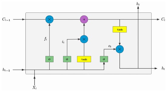
The LSTM network model framework is shown in Figure 1. $X_t$ represents the input information at time t, $C_t$ represents the unit state at time t, and $h_t$ represents the hidden state at time t.

Figure 1. The LSTM model structure.

2.2.2. The Gated Recurrent Unit (GRU) Model

In addition, Cho et al. [47] proposed the GRU model in 2014 as a variant of RNN networks, which showed excellent performance. Compared to the LSTM network, the structure of the GRU model is simpler and has fewer parameters, resulting in faster training speed. It is worth noting that LSTM networks and GRU networks are both derived from RNNs, so their internal unit structures are very similar. The difference is that the GRU network reduces one gating unit compared to the LSTM network, including only an update gate and a reset gate.

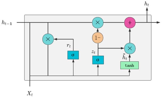
The GRU network model framework is shown in Figure 2. Where $z_t$ represents the update gate, $r_t$ represents the reset gate, ${\tilde{h}}_t$ is the sum of the input $x_t$ and the output result $h_{t-1}$ of the previous hidden layer.

Figure 2. The GRU model structure.

2.3. Sample Entropy (SampEn) Algorithm

SampEn is an algorithm for measuring the complexity of time series proposed by Richman et al. [48], which is an improvement over approximate entropy. It has the advantages of approximate entropy while avoiding the cumbersome process of self-matching and template matching, and eliminating the inconsistency of statistical quantities in approximate entropy. Compared with approximate entropy, SampEn has two advantages: it does not depend on the length of data for calculation, and it has better consistency. In addition, it also considers the information of the entire time series, can more fully reflect the complexity of the time series, and has a relatively simple calculation method, so it has wide applicability in practice. The specific steps are as follows:

(1)

Suppose $x\left(i\right)$ is a time series of length N, which can be constructed into a vector sequenc $X_m\left(1\right)$, …, $X_m(N-m+1)$ through it.

(2)

Define $d_{ij}[X\left(i\right),X\left(j\right)]$ (where $i\ne j$) as the absolute maximum difference between corresponding elements of $X_m\left(i\right)$ and $X_m\left(j\right)$.

(3)

Given a threshold r, the ratio of the number of $d_{ij}[X\left(i\right),X\left(j\right)]$≤ r to the total number is calculated and denoted as $B_r^m\left(i\right)$.

(4)

Calculate the average of all $B_r^m\left(i\right)$ values and name it $B^m\left(r\right)$. The calculation formula is as follows:

$$B^m\left(r\right)={\displaystyle \frac{1}{N-m}}\sum _{i=1}^{N-m}{B}_r^m\left(i\right)$$

(5)

(5)

Perform the repeated operations of steps (1) to (4) on the $(m+1)$-dimensional vector to obtain $B^{m+1}\left(r\right)$.

(6)

When N is a finite value, the estimated value of SampEn is:

$$SampEn(m,r,N)=-ln{\displaystyle \frac{B^{m+1}\left(r\right)}{B^m\left(r\right)}}$$

(6)

2.4. The Proposed Algorithm

To reasonably determine the window size and explore its impact on the performance of prediction models, this paper proposes a window size optimization strategy based on the SampEn algorithm (see Algorithm 1). This strategy aims to set the window size parameter appropriately, which is not only suitable for determining the window size of the original sequence but also effectively applicable to the determination of the window size for decomposed sequences, thus further enhancing prediction accuracy. The detailed steps and flowchart of the proposed algorithm are presented as follows:

(1)

Define a set of candidate window sizes, denoted as $W=\{w_1,w_2,\dots ,w_n\}$, where n represents the total number of candidate window sizes.

(2)

For each window size $w_i\in W$, apply the sliding window approach to the original data X to extract a set of window data sequences, denoted as $X_{w_i}^1,X_{w_i}^2,\dots ,X_{w_i}^m$, where m is the number of window data sequences that can be extracted for a given window size.

(3)

For each window data sequence $X_{w_i}^j$, compute its Sample Entropy (SampEn) value using the SampEn algorithm, denoted as $SampEn\left(X_{w_i}^j\right)$.

(4)

Calculate the mean (complexity) ${\mu }_{w_i}$ and standard deviation (volatility) ${\sigma }_{w_i}$ of the SampEn values for each window size $w_i$:

$${\mu }_{w_i}={\displaystyle \frac{1}{m}}\sum _{j=1}^{m}SampEn\left(X_{w_i}^j\right)$$

(7)

$${\sigma }_{w_i}=\sqrt{{\displaystyle \frac{1}{m}}\sum _{j=1}^m{\left(SampEn\left(X_{w_i}^j\right)-{\mu }_{w_i}\right)}^2}$$

(8)

(5)

Based on the specific requirements of the task or practical situation, assign weights $\alpha$ and $\beta$ (where $\alpha +\beta =1$) to the mean complexity ${\mu }_{w_i}$ and standard deviation (volatility) ${\sigma }_{w_i}$. Compute the combined coefficient $C_{w_i}$ for each window size $w_i$ using the weighted sum:

$$C_{w_i}=\alpha ·{\mu }_{w_i}+\beta ·{\sigma }_{w_i}$$

(9)

(6)

Select the window size $w_i$ that corresponds to the smallest combined coefficient $C_{w_i}$ as the optimal window size for the sliding window approach. This can be formally expressed as:

$$w_{\mathrm{final}}=\underset{w_i\in W}{\mathrm{argmin}}{C}_{w_i}$$

(10)

Algorithm 1: Optimal Window Size Selection using Sample Entropy

Require:        Dataset X, candidate window sizes $W=\{w_1,w_2,\dots ,w_n\}$ Ensure:        Optimal window size $w_{\mathrm{final}}$ 1: Define the set of candidate window sizes $W=\{w_1,w_2,\dots ,w_n\}$ 2: for $w_i\in W$ do 3:     Extract window data sequences $X_{w_i}^1,X_{w_i}^2,\dots ,X_{w_i}^m$ from the original data X using the sliding window approach 4:     for $X_{w_i}^j$ in the extracted window data sequences do 5:         Compute the Sample Entropy $SampEn\left(X_{w_i}^j\right)$ 6:     end for 7:     Compute the mean Sample Entropy ${\mu }_{w_i}$ for all window data sequences of size $w_i$ 8:     ${\mu }_{w_i}={\displaystyle \frac{1}{m}}{\sum }_{j=1}^{m}SampEn\left(X_{w_i}^j\right)$ 9:     Compute the standard deviation of Sample Entropy ${\sigma }_{w_i}$ for all window data sequences of size $w_i$ 10:     ${\sigma }_{w_i}=\sqrt{{\displaystyle \frac{1}{m}}{\sum }_{j=1}^m{(SampEn\left(X_{w_i}^j\right)-{\mu }_{w_i})}^2}$ 11:     Assign weights $\alpha$ and $\beta$ (where $\alpha +\beta =1$) to the mean complexity ${\mu }_{w_i}$ and standard deviation ${\sigma }_{w_i}$ 12:     Compute the combined coefficient $C_{w_i}$ for window size $w_i$ using the weighted sum 13:     $C_{w_i}=\alpha ·{\mu }_{w_i}+\beta ·{\sigma }_{w_i}$ 14: end for 15: Select the window size $w_i$ that corresponds to the smallest combined coefficient $C_{w_i}$ as the optimal window size $w_{\mathrm{final}}$ 16: $w_{\mathrm{final}}=\underset{w_i\in W}{\mathrm{argmin}}{C}_{w_i}$

2.5. Assessment Metric

In this article, we use the mean absolute error (MAE), root mean squared error (RMSE), and mean absolute percentage error (MAPE) as evaluation metrics. Their definitions are as follows:

$$RMSE=\sqrt{{\displaystyle \frac{1}{n}}\sum _{i=1}^n{(y_i-{\widehat{y}}_i)}^2}$$

(11)

$$MAPE={\displaystyle \frac{1}{n}}\sum _{i=1}^n{\displaystyle \frac{|y_i-{\widehat{y}}_i|}{y_i}}\times 100\%$$

(12)

$$MAE={\displaystyle \frac{1}{n}}\sum _{i=1}^n|y_i-{\widehat{y}}_i|$$

(13)

where n represents the length of the sequence, y and $\widehat{y}$, respectively, refer to the actual and predicted values.

3. Experimental Setup and Analysis

3.1. Data Set

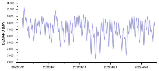
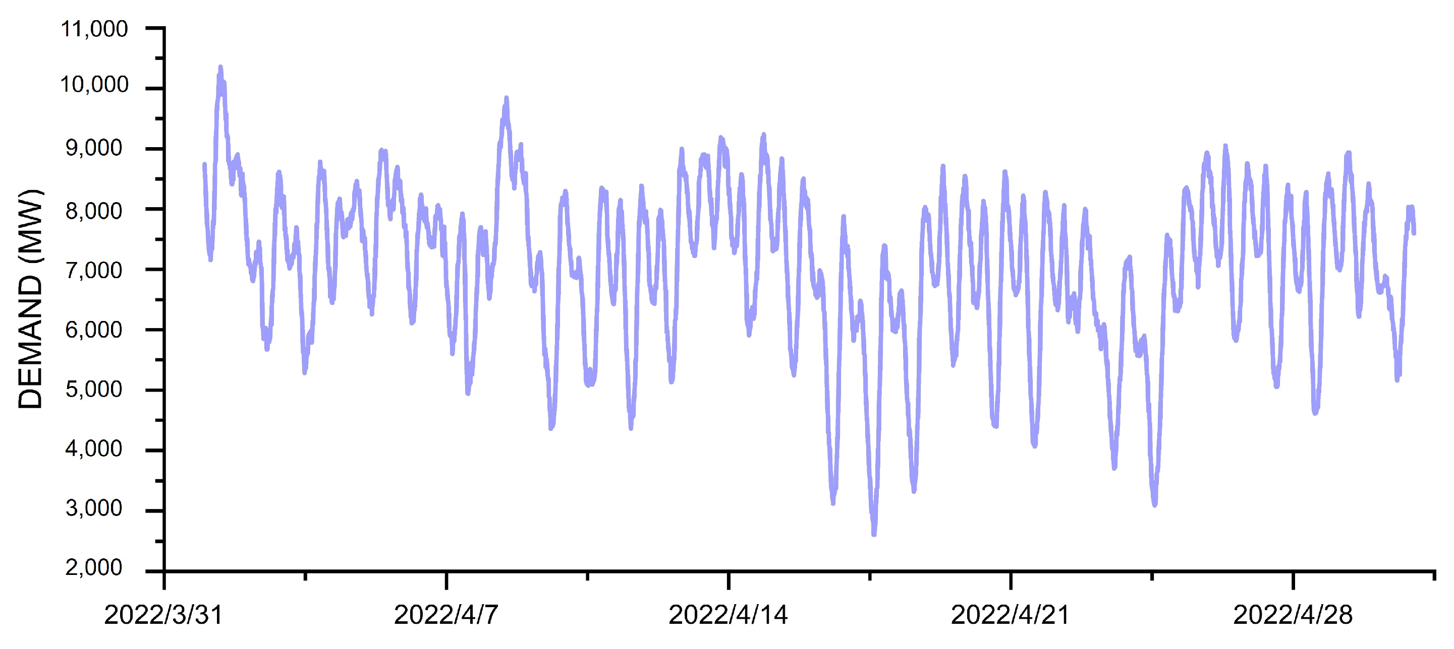
This study selects the open-source dataset from Elia GRID (https://opendata.elia.be/explore/dataset/ods003/information/ (accessed on 1 June 2024)) as the primary research subject. This dataset collects electricity load data from 1 April to 30 April 2022, with a sampling interval of 15 min, ensuring the timeliness and accuracy of the data. By observing Figure 3, it is not difficult to find that the data exhibits periodic characteristics. Particularly, the periodic fluctuations of the data are very prominent, which is closely related to people’s daily activity patterns.

Figure 3. Original power load series.

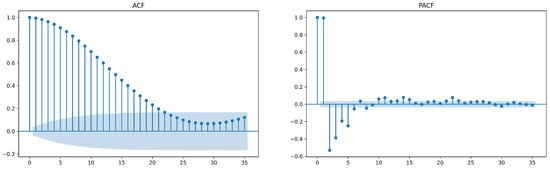
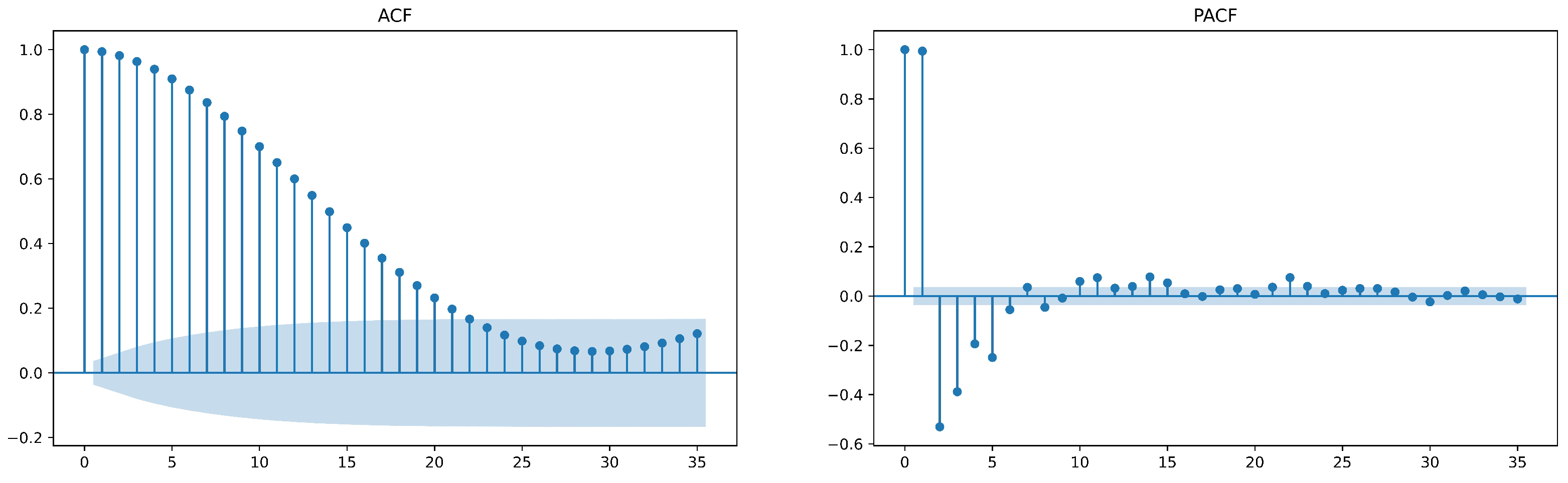
To gain a deeper understanding of the statistical properties of load data, this paper conducted tests and analyses on its stationarity, autocorrelation, and normality. The statistical test results are presented in Table 1. Firstly, the stationarity was evaluated using the Augmented Dickey-Fuller (ADF) test. The results showed that the p-value was 0.00, which is below the significance level of 0.05, thus rejecting the null hypothesis that the data series is stationary. Next, to explore the autocorrelation of the data, this paper employed the Autocorrelation Function (ACF), Partial Autocorrelation Function (PACF), and the Ljung–Box test. Based on the results in Table 1 and Figure 4, it can be concluded that there exists autocorrelation in the data. Finally, the normality of the data was tested using the Jarque–Bera test. The test results showed a p-value of 0.00, which is also below the significance level of 0.05, thus rejecting the null hypothesis and indicating that the data does not follow a normal distribution.

Table 1. Statistical test results of power load series.

Categories	p-Value	Hypothesis	Implication
ACF	N/A	N/A	Autocorrelation
PACF	N/A	N/A	Autocorrelation
ADF	0.00	Reject	Stationarity
Ljung–Box	0.00	Reject	Autocorrelation
Jarque–Bera	0.00	Reject	Non-normality

Note: N/A indicates Not Applicable, as the ACF and PACF do not provide a single p-value for hypothesis testing.

Figure 4. ACF and PACF result diagram.

The above results show that although the data are stationary, they contain a lot of noise with strong autocorrelation. In the face of this complex time series, traditional statistical models such as ARIMA and GARCH face great challenges in achieving accurate prediction modeling. Therefore, this paper introduces the frequency decomposition algorithm and neural network to optimize the prediction effect. The validation employs a two-stage, case-study design. Stage 1 (Case Study 1): The SampEn-based algorithm is applied to the undecomposed sequence to find the optimal window size, which then benchmarks models (RF, XGBoost, LSTM, GRU, Transformer). Stage 2 (Case Study 2): The algorithm is integrated into an EMD/CEEMD decomposition-reconstruction pipeline: it optimizes the window for each IMF component; components are forecast separately (LSTM/GRU/Transformer) and summed for the final prediction, enabling a comprehensive evaluation.

3.2. Case Study 1: Forecasting with Undecomposed Sequences

This case validates the window optimization algorithm on the original sequence. Procedure: (1) Apply the algorithm (Section 2.4) to find the optimal window from 86 to 106. (2) Build models (RF, XGBoost, LSTM, GRU, Transformer) using these optimal and baseline sizes. (3) Compare performance via MAE, RMSE, and MAPE to confirm the algorithm’s effectiveness.

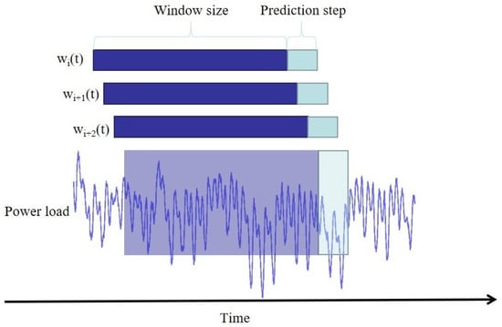
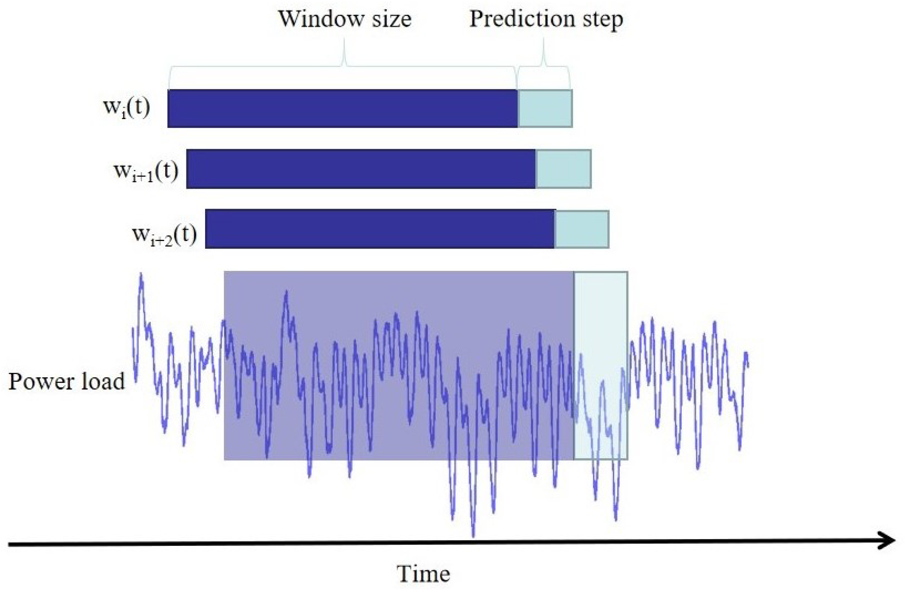
Figure 5 demonstrates the application of the sliding window method in electric power load forecasting. Faced with complex raw sequential data, the sliding window method divides these data into a series of interconnected segments in chronological order by setting a specific window size. Given an original sequence containing m data points, by setting the window size to n, we can obtain $m-n$ consecutive and overlapping window data segments, each containing n data points. These window data segments not only reflect the changing trends and characteristics of electric power load during specific periods, but also provide a valuable data foundation for the training of forecasting models. By learning the data correlations and patterns within each window segment, the model can more accurately predict future changes in electric power load. Therefore, the choice of window size is particularly crucial in the sliding window method, as it directly affects the range of data features that the model can capture, thus determining the accuracy and reliability of the forecasting results.

Figure 5. Sliding window method.

As a type of time series, power load data possesses its unique characteristics, the most prominent of which is periodicity. This periodicity is primarily influenced by multiple factors such as people’s daily habits, working patterns, seasonal changes, and weather patterns, making power load data occupy a special position in time series analysis. To accurately predict power load, it is necessary to consider its periodic characteristics and adopt appropriate data processing and analysis methods. Considering that the dataset used is sampled every 15 min, we initially chose 96 data points within a day as the window size. However, the choice of window size is not fixed and directly relates to the accuracy of the prediction model. To further enhance prediction accuracy, in this section, we introduce the SampEn algorithm to optimize and adjust the initial window size. Specifically, while maintaining the original window size of 96, we vary it by ±10 units, constructing a search space for window sizes ranging from 86 to 106. By applying the proposed algorithm, we search for a more suitable window size within this range, aiming to achieve more precise power load prediction results.

Our algorithm reveals the impact of window size changes on the complexity of the data sequence by calculating the mean SampEn of the window data sequence constructed under different window sizes. However, understanding complexity alone is insufficient. To further explore the overall picture of the window data sequence, we also calculate the standard deviation of its SampEn values under different window sizes, quantifying the degree of fluctuation in the data sequence. Nevertheless, we face a challenge in balancing the relationship between the mean SampEn (reflecting complexity) and the standard deviation (reflecting volatility). In the in-depth study of this section, after weighing up the options, we decided to assign a weight of 0.8 to the mean SampEn and a weight of 0.2 to the standard deviation. This weighting strategy aims to ensure that when evaluating window sizes, we can capture the complexity features of the data while not neglecting the important information about its volatility. Through this weight setting, we can more scientifically evaluate the data characteristics under different window sizes, thereby selecting a reasonable window size to construct an accurate power load prediction model.

After calculation, we obtained specific values of the mean SampEn, standard deviation, and comprehensive coefficient for different window sizes, as detailed in Table 2. Among these window sizes, the window size with the smallest comprehensive coefficient is 106, while the size with the largest comprehensive coefficient is 86.

Table 2. Numerical results corresponding to different window sizes.

Window Size	Mean	Rank	S.D.	Rank	Coefficient	Rank
86	0.33873	7	0.10786	21	0.29256	21
87	0.33862	5	0.10707	20	0.29231	20
88	0.33860	4	0.10664	19	0.29221	19
89	0.33844	2	0.10597	18	0.29194	17
90	0.33826	1	0.10503	17	0.29162	6
91	0.33858	3	0.10421	16	0.29170	10
92	0.33866	6	0.10356	15	0.29164	8
93	0.33878	8	0.10319	14	0.29166	9
94	0.33884	9	0.10280	13	0.29163	7
95	0.33917	11	0.10231	12	0.29180	12
96	0.33944	13	0.10183	11	0.29192	16
97	0.33964	16	0.10118	10	0.29194	18
98	0.33968	17	0.10067	9	0.29188	15
99	0.33978	19	0.10027	8	0.29188	14
100	0.33983	20	0.09977	7	0.29182	13
101	0.33984	21	0.09940	6	0.29176	11
102	0.33973	18	0.09903	5	0.29159	5
103	0.33960	15	0.09878	4	0.29144	4
104	0.33951	14	0.09850	3	0.29130	3
105	0.33930	12	0.09809	2	0.29106	2
106	0.33906	10	0.09766	1	0.29078	1

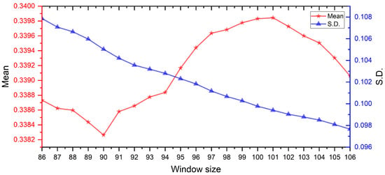
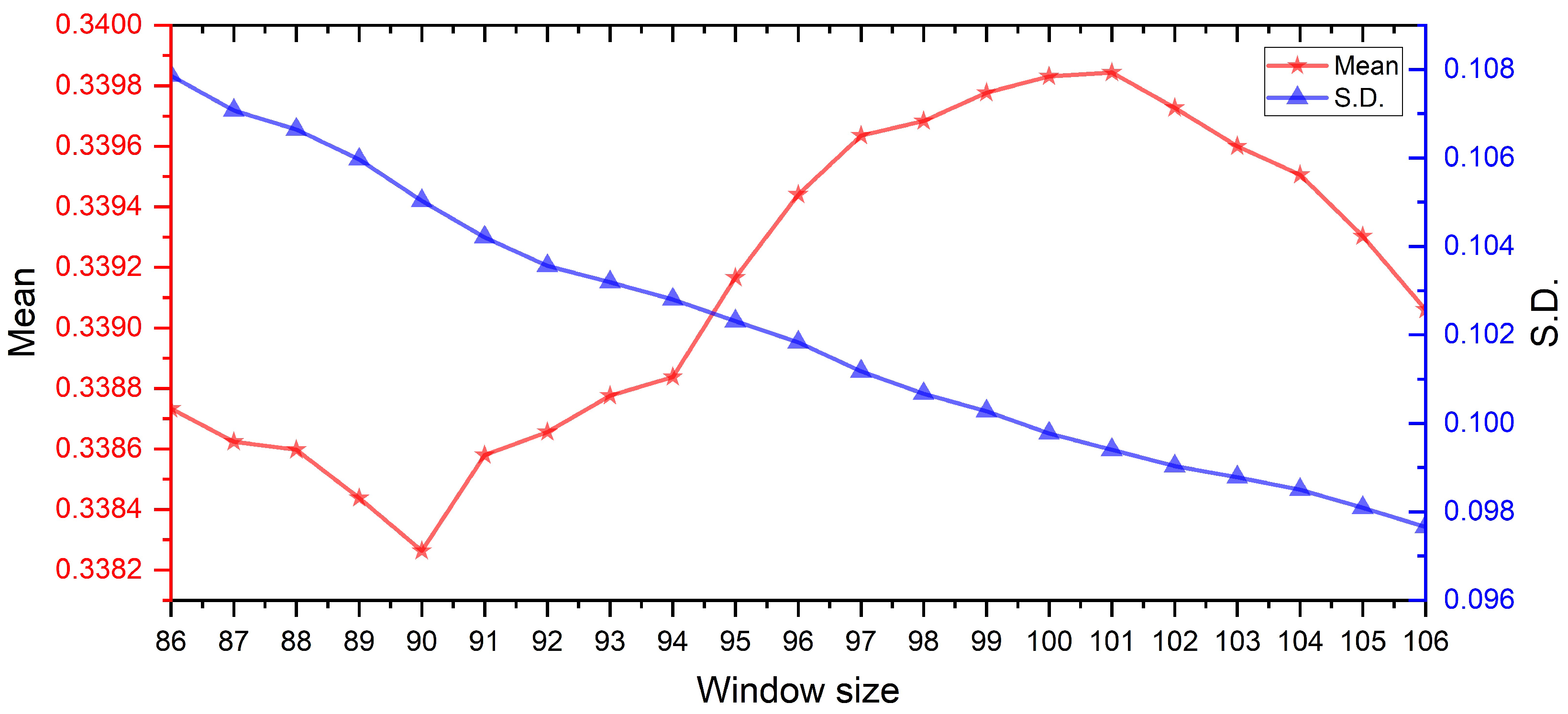
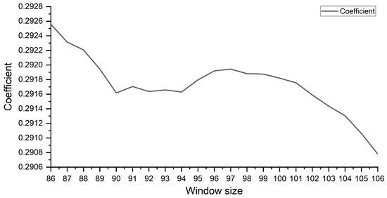
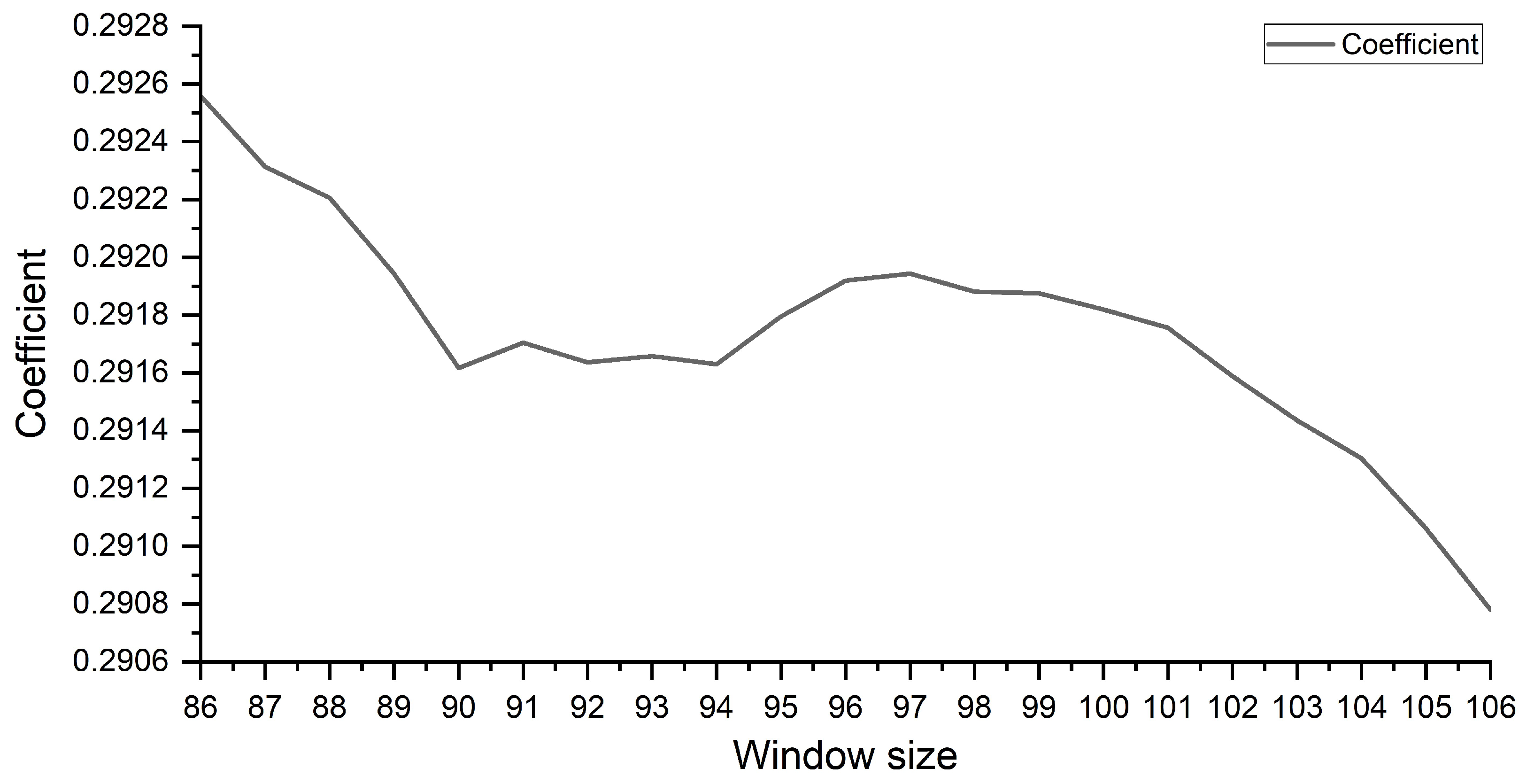
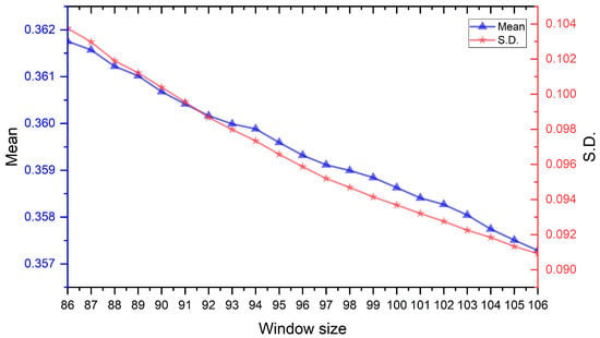
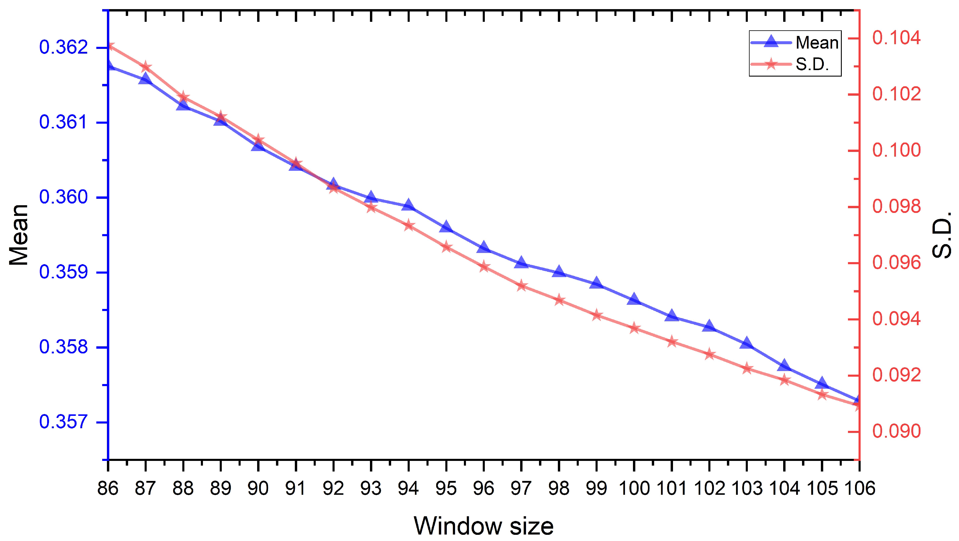
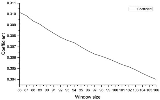
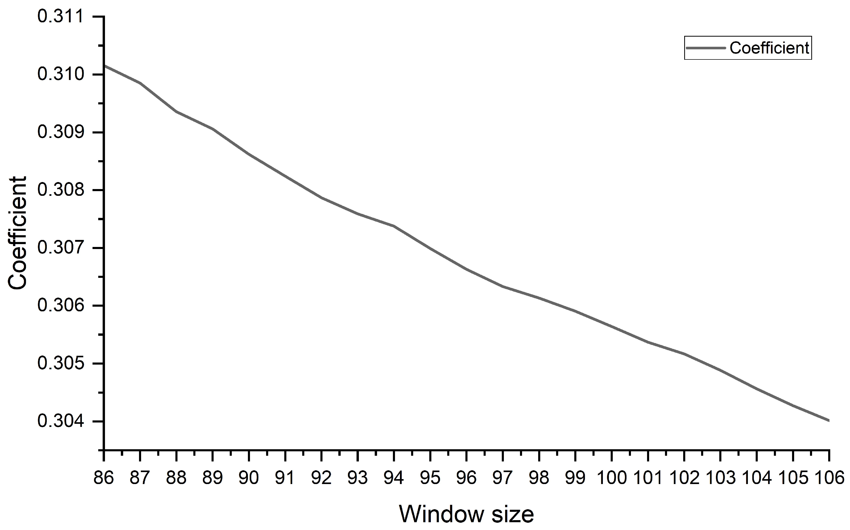
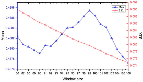
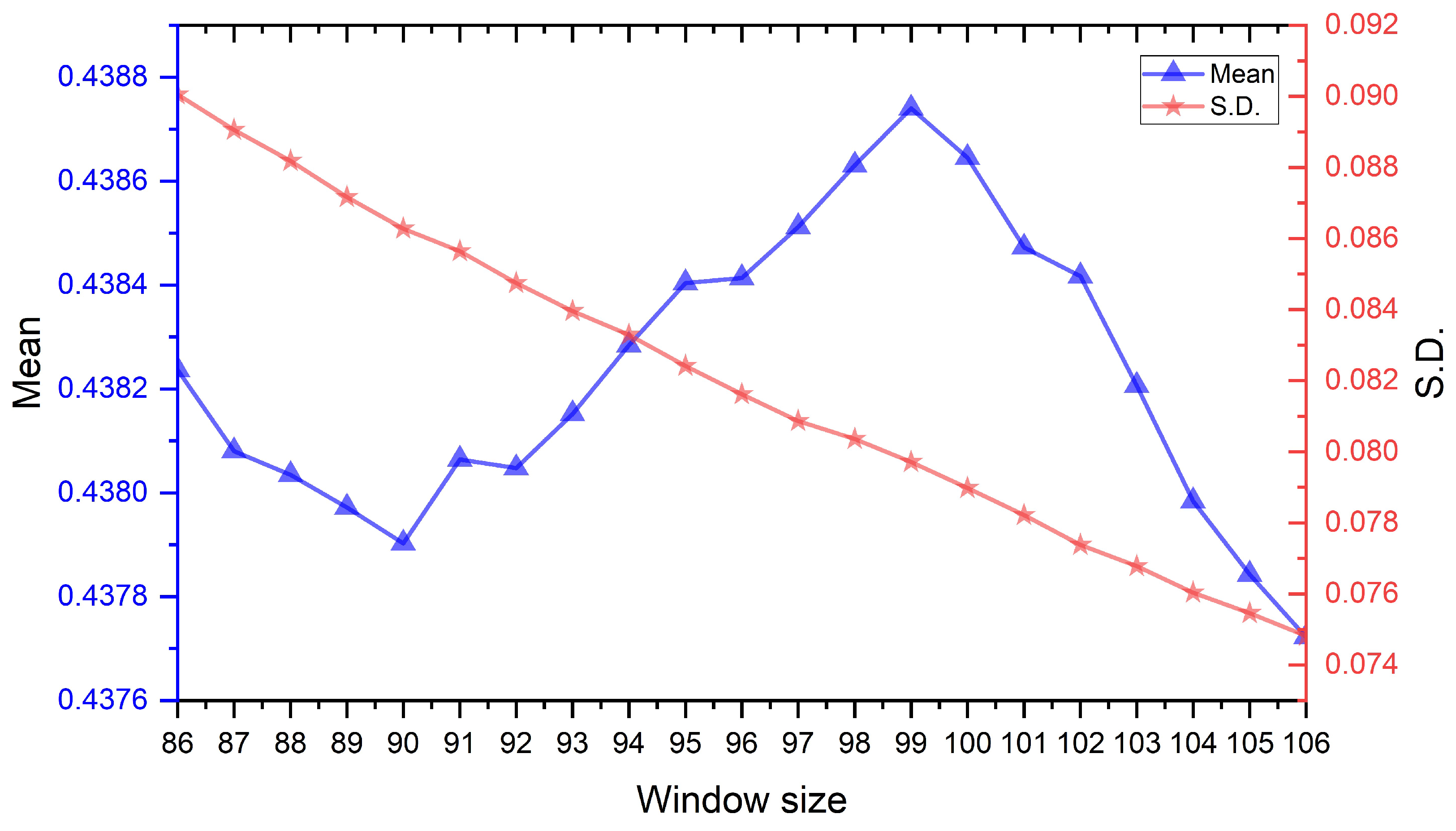
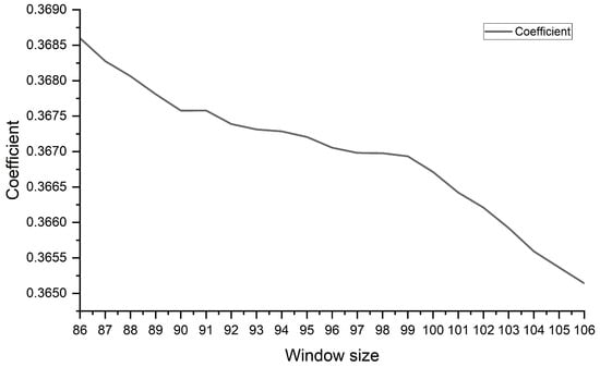
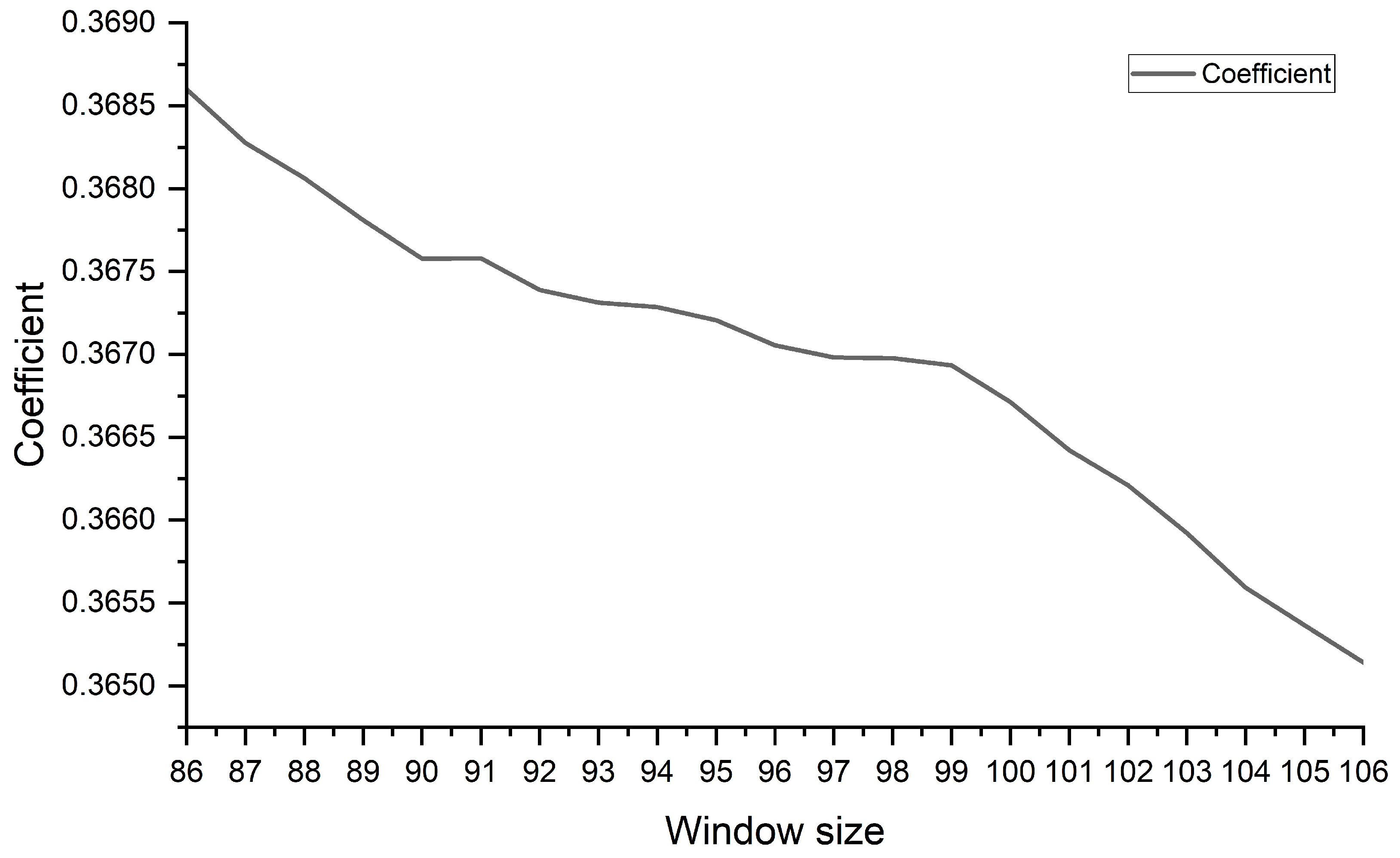
To more intuitively reveal the differences between them, we conducted a visualization process. The mean and standard deviation of SampEn are presented in Figure 6, while the comprehensive coefficient is shown in Figure 7. From Figure 6, it is clearly observable that as the window size gradually changes, the mean SampEn of the window data series exhibits a series of variations: initially, it declines, then gradually rises, and finally decreases again. This trend profoundly reveals the diversity of data sequence complexity under different window sizes. Notably, when the window size is set to 101, the mean SampEn reaches a peak of 0.33984, while it drops to a trough of 0.33826 when the window size is 90. Although changes in the window size indeed affect the mean SampEn, this difference is not significant. The gap between the maximum and minimum values is only 0.001581, reflecting the relatively stable characteristics of data sequence complexity under different window sizes. In contrast, the standard deviation gradually decreases as the window size increases, a trend that does not align with the changes in the mean SampEn. Additionally, by observing Figure 6, we can find that the comprehensive coefficient exhibits a similar fluctuating trend to the mean SampEn.

Figure 6. Mean and S.D. corresponding to different window sizes.

Figure 7. Coefficients corresponding to different window sizes.

To evaluate the feasibility and effectiveness of our proposed algorithm more objectively, we conducted experiments using various methods from the field of machine learning and neural networks. These methods include Random Forest (RF), XGBoost, GRU, and LSTM models. Their respective prediction accuracies are presented in Table 3, Table 4 and Table 5.

Table 3. MAE Index values of different models.

Window Size	GRU	Rank	LSTM	Rank	XGBoost	Rank	RF	Rank	Mean Rank
86	81.249	21	80.303	21	83.070	5	81.499	9	14
87	79.368	16	79.994	20	84.152	7	82.310	17	15
88	78.847	12	77.905	8	86.254	15	81.715	10	11.25
89	78.695	9	78.299	13	84.634	8	82.695	21	12.75
90	79.144	13	77.850	5	86.887	19	82.651	20	14.25
91	80.686	19	77.911	9	87.077	20	81.765	13	15.25
92	80.193	18	77.793	4	88.143	21	82.479	18	15.25
93	79.287	15	77.880	7	85.844	13	82.649	19	13.5
94	79.763	17	79.129	15	86.769	18	81.757	11	15.25
95	81.075	20	79.944	19	85.983	14	81.872	14	16.75
96	78.731	11	79.334	17	85.570	11	82.158	16	13.75
97	79.250	14	78.635	14	86.684	17	82.133	15	15
98	78.722	10	77.867	6	83.035	4	81.761	12	8
99	77.608	3	79.568	18	86.470	16	81.219	6	10.75
100	78.311	7	79.274	16	85.345	10	81.405	8	10.25
101	77.990	6	78.208	12	83.802	6	80.566	1	6.25
102	78.582	8	78.006	10	82.739	3	81.167	5	6.5
103	77.883	5	77.630	3	85.802	12	80.942	4	6
104	77.584	2	78.077	11	82.442	1	81.245	7	5.25
105	77.782	4	77.612	2	84.951	9	80.714	3	4.5
106	77.204	1	77.303	1	82.650	2	80.712	2	1.5

Table 4. RMSE Index values of different models.

Window Size	GRU	Rank	LSTM	Rank	XGBoost	Rank	RF	Rank	Mean Rank
86	100.387	17	100.525	18	103.937	2	101.648	8	11.25
87	98.328	13	101.284	20	105.843	8	102.370	12	13.25
88	97.753	9	98.050	11	107.574	12	101.641	7	9.75
89	97.901	10	96.921	3	106.919	11	102.545	14	9.5
90	100.394	18	98.058	12	108.657	18	102.938	20	17
91	101.228	21	97.448	7	108.909	20	102.383	13	15.25
92	101.178	20	97.767	9	109.321	21	102.791	17	16.75
93	99.256	15	98.215	14	107.842	15	103.113	21	16.25
94	100.699	19	100.040	16	107.700	13	102.736	16	16
95	99.958	16	101.363	21	108.192	17	102.927	19	18.25
96	97.657	7	100.389	17	107.800	14	102.870	18	14
97	97.935	11	97.351	5	107.965	16	102.668	15	11.75
98	97.395	6	97.232	4	104.321	3	102.074	11	6
99	97.392	5	100.536	19	108.812	19	101.715	9	13
100	98.757	14	98.922	15	106.675	9	101.963	10	12
101	97.265	2	98.201	13	105.246	6	100.958	1	5.5
102	97.334	4	97.617	8	104.923	4	101.501	5	5.25
103	97.270	3	96.839	2	106.785	10	101.384	4	4.75
104	97.659	8	97.998	10	105.094	5	101.601	6	7.25
105	98.204	12	96.795	1	105.622	7	101.183	3	5.75
106	97.054	1	97.386	6	103.237	1	101.125	2	2.5

Table 5. Detailed MAPE results for different models.

Window Size	GRU	Rank	LSTM	Rank	XGBoost	Rank	RF	Rank	Mean Rank
86	1.138	20	1.123	21	1.165	5	1.138	8	11.25
87	1.114	15	1.111	17	1.176	7	1.150	17	13.25
88	1.106	12	1.094	10	1.207	15	1.141	10	9.75
89	1.103	9	1.097	13	1.187	9	1.158	21	9.5
90	1.108	13	1.088	4	1.215	20	1.156	20	17
91	1.135	19	1.092	8	1.211	18	1.141	11	15.25
92	1.120	18	1.089	5	1.233	21	1.153	18	16.75
93	1.113	14	1.091	6	1.198	12	1.155	19	16.25
94	1.115	17	1.110	16	1.213	19	1.144	12	16
95	1.140	21	1.113	19	1.203	14	1.145	14	18.25
96	1.104	10	1.112	18	1.195	11	1.148	15	14
97	1.115	16	1.102	14	1.210	17	1.148	16	11.75
98	1.104	11	1.094	12	1.158	4	1.144	13	6
99	1.086	2	1.114	20	1.208	16	1.135	6	13
100	1.096	7	1.109	15	1.193	10	1.139	9	12
101	1.094	6	1.094	11	1.172	6	1.126	1	5.5
102	1.102	8	1.092	7	1.156	3	1.134	5	5.25
103	1.092	5	1.086	3	1.198	13	1.133	4	4.75
104	1.087	3	1.093	9	1.150	1	1.136	7	7.25
105	1.089	4	1.086	2	1.181	8	1.129	2	5.75
106	1.082	1	1.078	1	1.151	2	1.129	3	2.5

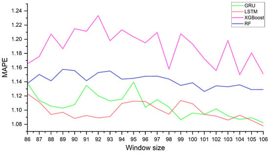
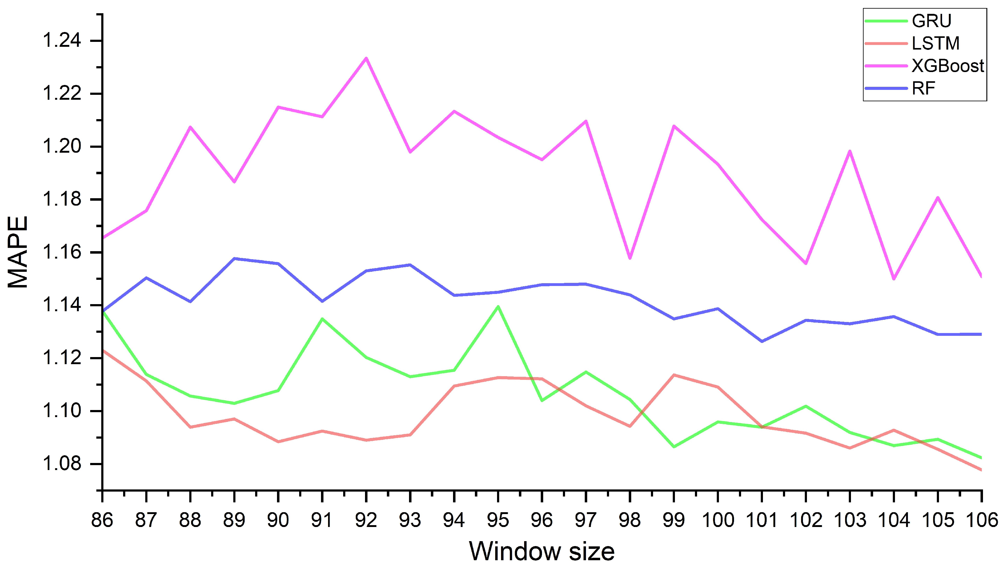
From Table 3, Table 4 and Table 5, we can clearly observe that there are differences in the predictive accuracy index values corresponding to different window sizes. We further visualized the predictive accuracy index values to more intuitively demonstrate their changing trends with the window size. As shown in Figure 8 (MAPE), the predictive accuracy exhibits significant fluctuations as the window size changes and does not vary monotonically. This non-monotonic trend is consistently observed across all evaluation metrics (MAE, RMSE, and MAPE), as detailed in the numerical results presented in Table 3, Table 4 and Table 5.

Figure 8. Visual comparison of MAPE values across different models.

When the window size was set to 106, the GRU model performed exceptionally well according to the MAE metric, with an MAE value of 77.204. At the same window size, the LSTM model also performed well, achieving an MAE score of 77.304, which is nearly equal to the ideal GRU model. With an MAE value of 81.249, the GRU model with a window size of 86, however, did not do very well. Its prediction accuracy dropped by 4.045, or over 5%, in comparison to the best GRU model. Furthermore, the prediction accuracy decreased by 1.527, or 1.94%, in comparison to the original GRU model with a window size of 96, which had an MAE value of 78.731. These comparative data indicate that the window size significantly impacts the model’s prediction accuracy, and selecting an appropriate window size is crucial for enhancing model performance. This trend applies not only to the MAE metric but also to the RMSE and MAPE metrics.

Furthermore, we discovered notable variations in prediction performance among the XGBoost algorithm, RF model, and neural network models by examining the numerical data in Table 3, Table 4 and Table 5. This discrepancy demonstrates how differently they handle complex data and emphasizes the benefit of neural network models for handling nonlinear data. The RMSE and MAPE measurements also show this performance gap, which supports the neural network models’ exceptional data prediction capabilities.

We investigated to assess how well various window sizes performed across a range of models and indicators. Using the MAE measure as an example, Table 3 shows that it performed best among the GRU and LSTM models when the window size was 106. The XGBoost technique and RF model came in second and third, respectively. We determined each model’s average performance under this window size and came up with a comprehensive score of 1.5, which indicates good performance. On the other hand, it nevertheless placed second in the LSTM and RF models, fourth in the GRU model, and ninth in the XGBoost method, with a total score of 4.5, even though overall performance was marginally worse when the window size was 105.

Additionally, when the window size was 106, the comprehensive scores under the RMSE and MAPE measures were 2.25 and 1.75, respectively, showing both good prediction performance. These experimental findings confirm the efficacy and viability of the suggested method in addition to demonstrating the logic of choosing a window size of 106. A window size of 106 consistently demonstrated exceptional prediction performance across a range of methods and evaluation metrics.

Also, we discovered that prediction results might be impacted by the selection of the prediction model and loss function. Therefore, depending on particular data properties and problem settings, it is vital to carefully choose appropriate loss functions and prediction models in real-world applications. This method can improve the accuracy and dependability of data analysis, further optimize model prediction performance, and more effectively satisfy real-world requirements.

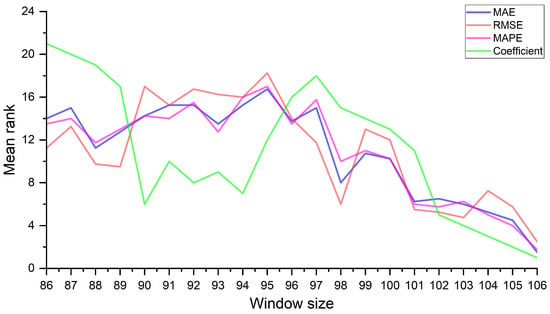
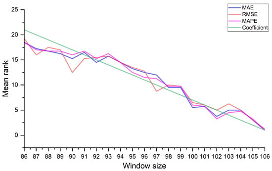
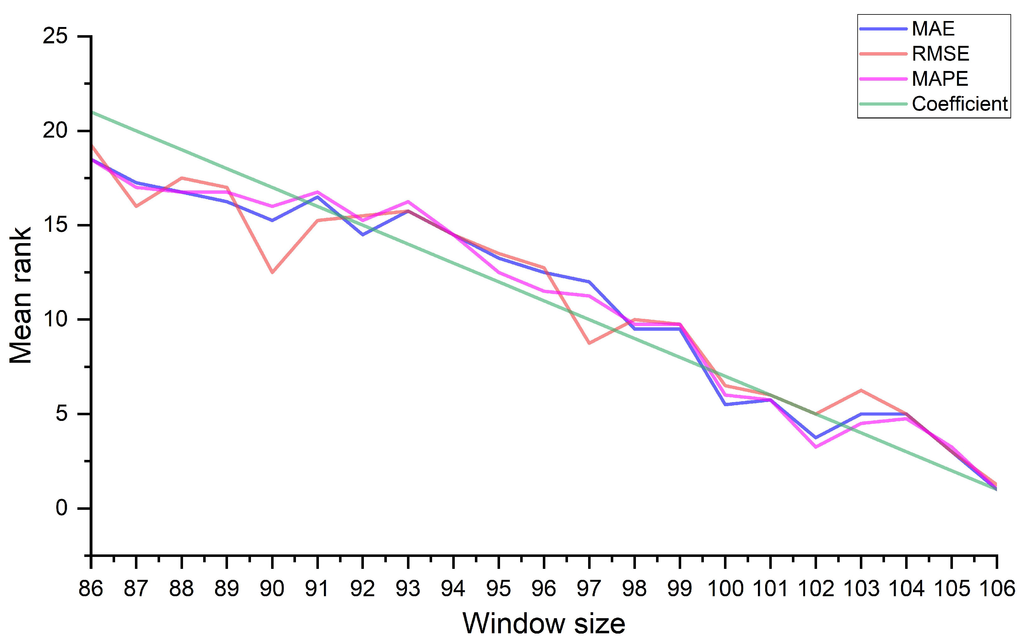
We visualized the comprehensive coefficient for different window sizes and their overall performance under various evaluation metrics, as shown in Figure 9. From Figure 9, we can observe a certain alignment between the overall performance trends of the evaluation metrics and the changes in the comprehensive coefficients, providing a reference for selecting appropriate window sizes. However, there are also some special cases, such as when the window size is 90, where, despite a relatively low comprehensive coefficient, the performance under various evaluation metrics is unsatisfactory. This phenomenon suggests that apart from the window size, there may be other unknown factors influencing the construction of the prediction model, which we have not yet considered. Therefore, when using the proposed algorithm, we recommend setting a broader range of alternative window sizes to avoid potential decreases in prediction performance due to special circumstances. In future research, we will further explore the reasons for this situation to optimize the prediction model construction process more comprehensively, improving prediction accuracy and stability.

Figure 9. Rank of different window sizes.

In this section, we verified the efficacy of the suggested technique by applying it to the sequence data of the undecomposed electric load. The suggested algorithm’s viability and logic were validated by comparing the experimental outcomes of several models and evaluation criteria. In the meantime, the experiment showed that the model’s prediction accuracy will be impacted by the window size choice. Furthermore, the mean value of SampEn shows a fluctuating feature rather than a single changing trend as the window size progressively increases. At the same time, SampEn’s standard deviation shows a clearly different trend, namely a progressive decline. Because of this, the comprehensive coefficient shows a trend of fluctuation that is comparable to that of the SampEn mean value. Therefore, when determining the appropriate window size, we must comprehensively consider the complexity and volatility of the data to find the best balance. In the Section 3.3, we will further explore the practical application of the proposed method in sequence decomposition. Through verification, we will evaluate the effectiveness and practicality of this method, providing practical guidance for solving actual problems. To further benchmark our method against contemporary architectures, we evaluated the Transformer model. The Transformer model also attained its optimal performance at a window size of 106 for the undecomposed sequence, with MAE, RMSE, and MAPE values of 77.21, 96.91, and 1.085. This result is noteworthy as it independently corroborates the optimality of the window size identified by our SampEn-based algorithm across a radically different model paradigm. While the Transformer’s accuracy is excellent, the GRU and LSTM models offer a compelling balance of high performance, lower training cost, and simpler architecture, making them highly practical for the task at hand.

3.3. Case Study 2: Forecasting with Decomposed Sequences

This case evaluates the algorithm within a decomposition-reconstruction pipeline. Steps: (1) Decompose the series using EMD/CEEMD (Section 2.1). (2) Determine the optimal window for each IMF. (3) Forecast components with LSTM, GRU, and Transformer models. (4) Reconstruct the final prediction by summation. (5) Compare accuracy against the undecomposed baseline to highlight the synergy between decomposition and adaptive window sizing.

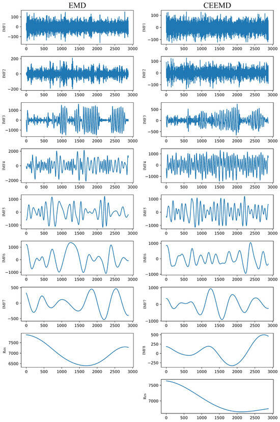
We employed both EMD and CEEMD algorithms to process the original electric power load sequence, obtaining their respective component sequences. The decomposition results are shown in Figure 10. Specifically, the EMD algorithm decomposed the original sequence into 8 component sequences, while the CEEMD algorithm, an optimized version of EMD, achieved a more refined decomposition by introducing complementary white noise data, ultimately generating 9 component sequences. Due to the introduction of this optimization step, CEEMD and EMD exhibit differences in the decomposition process, leading to varying numbers of component sequences. These component sequences not only represent different components and characteristics of the original sequence but also play a crucial role in building prediction models. The training process of the model is significantly influenced by these component sequences, as they provide distinct data features and patterns that enable the model to comprehensively learn and understand the intrinsic laws of the data. Additionally, prediction results may vary due to differences in component sequences, further emphasizing their importance in the prediction process. Therefore, when selecting and applying different decomposition algorithms, we need to consider their characteristics and impacts to better utilize component sequences in building and optimizing prediction models, thus achieving more accurate and reliable prediction results. Through a comparative analysis of EMD and CEEMD algorithms, we can gain a deeper understanding of their application effects in the decomposition of electric power load sequences.

Figure 10. Decomposition results of different decomposition algorithms.

To further analyze the characteristics of these component sequences, we calculated their SampEn means and standard deviations under different window sizes. To ensure consistency and fairness in the comparison, we maintained the same weights as in the undecomposed sequence during the calculation process. We have organized these detailed data into Table 6 and Table 7 for subsequent in-depth analysis and comparison. Moreover, to visually reveal the characteristics of these results, we conducted fine-grained visualization processing and presented the results in graphical form in Figure 11, Figure 12, Figure 13 and Figure 14.

Table 6. Calculation results corresponding to different window sizes of the EMD algorithm.

Window Size	Mean	Rank	S.D.	Rank	Coefficient	Rank
86	0.36175	21	0.10376	21	0.31015	21
87	0.36157	20	0.10297	20	0.30985	20
88	0.36122	19	0.10190	19	0.30936	19
89	0.36102	18	0.10122	18	0.30906	18
90	0.36068	17	0.10039	17	0.30862	17
91	0.36041	16	0.09955	16	0.30824	16
92	0.36017	15	0.09868	15	0.30787	15
93	0.35999	14	0.09799	14	0.30759	14
94	0.35988	13	0.09734	13	0.30738	13
95	0.35959	12	0.09658	12	0.30699	12
96	0.35932	11	0.09587	11	0.30663	11
97	0.35912	10	0.09520	10	0.30633	10
98	0.35899	9	0.09469	9	0.30613	9
99	0.35884	8	0.09415	8	0.30591	8
100	0.35863	7	0.09369	7	0.30564	7
101	0.35841	6	0.09321	6	0.30537	6
102	0.35827	5	0.09276	5	0.30517	5
103	0.35804	4	0.09225	4	0.30488	4
104	0.35774	3	0.09185	3	0.30457	3
105	0.35751	2	0.09133	2	0.30427	2
106	0.35729	1	0.09093	1	0.30401	1

Table 7. Calculation results corresponding to different window sizes of the CEEMD algorithm.

Window Size	Mean	Rank	S.D.	Rank	Coefficient	Rank
86	0.43824	12	0.09005	21	0.36860	21
87	0.43808	9	0.08906	20	0.36828	20
88	0.43803	6	0.08818	19	0.36806	19
89	0.43797	4	0.08716	18	0.36781	18
90	0.43790	3	0.08628	17	0.36758	16
91	0.43806	8	0.08564	16	0.36758	17
92	0.43805	7	0.08475	15	0.36739	15
93	0.43815	10	0.08396	14	0.36731	14
94	0.43828	13	0.08329	13	0.36729	13
95	0.43840	14	0.08241	12	0.36721	12
96	0.43841	15	0.08162	11	0.36705	11
97	0.43851	18	0.08087	10	0.36698	10
98	0.43863	19	0.08036	9	0.36698	9
99	0.43874	21	0.07971	8	0.36693	8
100	0.43864	20	0.07898	7	0.36671	7
101	0.43847	17	0.07822	6	0.36642	6
102	0.43842	16	0.07738	5	0.36621	5
103	0.43821	11	0.07678	4	0.36592	4
104	0.43798	5	0.07603	3	0.36559	3
105	0.43784	2	0.07546	2	0.36537	2
106	0.43772	1	0.07482	1	0.36514	1

Figure 11. Mean and S.D. of EMD algorithm with different window sizes.

Figure 12. Coefficient of EMD algorithm with different window sizes.

Figure 13. Mean and S.D. of CEEMD algorithm with different window sizes.

Figure 14. Coefficient of CEEMD algorithm with different window sizes.

Observing Figure 11, we can clearly see that as the window size gradually increases, both the mean and standard deviation of the SampEn for the EMD algorithm exhibit a relatively stable downward trend. This trend indicates that as the window size grows, the complexity of the data processed by the EMD algorithm gradually decreases, and the degree of data dispersion also diminishes, exhibiting more stable characteristics. However, the trend of the SampEn mean of the CEEMD algorithm differs from the EMD algorithm, showing a fluctuating and undulating pattern as the window size gradually increases, revealing more complex dynamic properties. Similar to the EMD algorithm, the standard deviation of the CEEMD algorithm also exhibits a gradual decrease during the process of increasing the window size. These results demonstrate that different decomposition algorithms yield different SampEn means when processing the same data.

According to the numerical results in Table 6 and Table 7, our proposed algorithm suggests that a window size of 106 is a reasonable choice. To validate the practical application effectiveness of the proposed algorithm in decomposing sequences, we further conducted an in-depth study on the prediction accuracy of LSTM and GRU models under different evaluation metrics for various decomposition algorithms with different window sizes. Through this analysis, we can comprehensively assess the performance and advantages of the proposed algorithm.

Furthermore, by observing Figure 13 and Figure 14, we notice that although the comprehensive coefficients of both algorithms gradually decrease with the increase in the window size, they exhibit contrasting trends in terms of the SampEn mean of the component sequences. Specifically, the SampEn mean of the component sequences obtained by the EMD algorithm gradually decreases as the window size increases, exhibiting a stable downward trend. In contrast, the SampEn mean of the component sequences obtained by the CEEMD algorithm exhibits a fluctuating pattern, indicating a more complex and diverse variation in its SampEn.

Table 8, Table 9 and Table 10 present the prediction results of the combined decomposition algorithm and neural network models, including MAE, RMSE, and MAPE as metrics for prediction accuracy. Upon careful examination, it is evident that both the EMD and CEEMD algorithms have significantly improved the prediction accuracy of neural network models compared to the original undecomposed series. Taking MAE as an example, the average MAE values for LSTM and GRU models without decomposition are 78.638 and 78.950, respectively. However, after introducing the EMD and CEEMD algorithms, the prediction accuracy of the neural network models has been notably enhanced. Specifically, the average MAE values of EMD-LSTM, EMD-GRU, CEEMD-LSTM, and CEEMD-GRU have been reduced to 41.966, 38.415, 21.086, and 19.407, respectively. Compared to the corresponding models without decomposition, these decomposed models have achieved remarkable improvements in MAE values, with average reductions of 36.984, 40.223, 57.864, and 59.231, respectively, representing accuracy enhancements of 36.984%, 40.223%, 57.864%, and 59.231%, respectively. This empirical result not only validates the practicability of decomposition algorithms in time series analysis but also highlights their immense potential and practical value in improving prediction accuracy. By selecting and applying decomposition algorithms appropriately, we can enhance the predictive performance of neural network models, thus providing more accurate and reliable prediction results for practical applications.

Table 8. The value of the MAE index predicted by the decomposition algorithm.

Window Size	EMD-LSTM		EMD-GRU		CEEMD-LSTM		CEEMD-GRU		Mean Rank
	Value	Rank	Value	Rank	Value	Rank	Value	Rank
86	42.987	20	39.348	17	22.154	18	20.758	19	18.5
87	42.957	19	39.563	19	21.137	11	20.865	20	17.25
88	42.479	13	39.472	18	22.470	21	19.937	15	16.75
89	42.212	10	39.725	20	21.653	14	20.966	21	16.25
90	42.232	11	39.870	21	21.649	13	19.959	16	15.25
91	42.638	16	39.205	16	21.970	17	20.005	17	16.5
92	42.734	17	38.472	10	22.283	19	19.503	12	14.5
93	43.625	21	38.605	13	21.835	15	19.884	14	15.75
94	42.569	14	38.535	11	22.400	20	19.527	13	14.5
95	42.423	12	38.827	15	21.852	16	19.204	10	13.25
96	42.842	18	38.030	9	21.630	12	19.265	11	12.5
97	42.586	15	37.922	8	20.597	7	20.145	18	12
98	41.781	9	38.675	14	20.374	6	19.201	9	9.5
99	41.699	8	38.562	12	20.890	10	19.066	8	9.5
100	41.422	7	37.279	2	20.729	9	18.540	4	5.5
101	41.400	6	37.691	6	20.044	5	18.588	6	5.75
102	40.968	5	37.300	3	20.034	4	18.324	3	3.75
103	40.414	2	37.592	5	20.601	8	18.562	5	5
104	40.461	3	37.790	7	19.712	3	18.759	7	5
105	40.719	4	37.368	4	19.572	2	18.313	2	3
106	40.137	1	36.889	1	19.215	1	18.186	1	1

Table 9. The value of the RMSE index predicted by the decomposition algorithm.

Window Size	EMD-LSTM		EMD-GRU		CEEMD-LSTM		CEEMD-GRU		Mean Rank
	Value	Rank	Value	Rank	Value	Rank	Value	Rank
86	57.839	21	52.457	21	27.225	16	25.600	19	19.25
87	56.214	13	52.328	20	26.432	11	25.693	20	16
88	57.563	19	51.503	16	27.699	19	24.637	16	17.5
89	57.202	17	51.949	18	26.502	12	25.962	21	17
90	54.501	4	52.018	19	26.653	13	24.356	14	12.5
91	56.131	12	51.330	14	27.387	17	24.763	18	15.25
92	57.036	16	51.363	15	27.532	18	24.341	13	15.5
93	57.431	18	50.427	9	27.772	21	24.512	15	15.75
94	56.879	14	51.036	12	27.731	20	24.060	12	14.5
95	56.924	15	51.744	17	26.859	14	23.347	8	13.5
96	57.565	20	50.039	6	27.118	15	23.875	10	12.75
97	54.459	3	50.337	8	25.442	7	24.682	17	8.75
98	55.667	10	51.105	13	25.394	6	23.964	11	10
99	55.625	9	50.992	11	26.049	10	23.588	9	9.75
100	55.334	7	49.758	4	25.829	8	23.128	7	6.5
101	56.003	11	49.918	5	25.120	4	22.915	4	6
102	55.388	8	49.316	2	25.183	5	22.925	5	5
103	55.294	6	50.159	7	25.942	9	22.892	3	6.25
104	54.381	1	50.443	10	24.456	3	23.126	6	5
105	54.809	5	49.678	3	24.422	2	22.537	2	3
106	54.418	2	48.599	1	23.992	1	22.529	1	1.25

Table 10. The value of the MAPE index predicted by the decomposition algorithm.

Window Size	EMD-LSTM		EMD-GRU		CEEMD-LSTM		CEEMD-GRU		Mean Rank
	Value	Rank	Value	Rank	Value	Rank	Value	Rank
86	0.607	20	0.548	16	0.311	18	0.294	20	18.5
87	0.607	19	0.552	19	0.297	11	0.289	19	17
88	0.602	15	0.552	18	0.317	20	0.277	14	16.75
89	0.598	13	0.559	20	0.305	13	0.295	21	16.75
90	0.589	10	0.560	21	0.307	17	0.280	16	16
91	0.605	18	0.551	17	0.306	14	0.281	18	16.75
92	0.603	16	0.539	11	0.319	21	0.276	13	15.25
93	0.615	21	0.541	13	0.307	16	0.279	15	16.25
94	0.604	17	0.539	10	0.313	19	0.272	12	14.5
95	0.595	11	0.544	15	0.306	15	0.270	9	12.5
96	0.599	14	0.533	9	0.299	12	0.271	11	11.5
97	0.597	12	0.531	8	0.291	8	0.281	17	11.25
98	0.588	8	0.543	14	0.288	7	0.271	10	9.75
99	0.589	9	0.540	12	0.293	10	0.267	8	9.75
100	0.582	7	0.523	3	0.291	9	0.260	5	6
101	0.582	6	0.528	6	0.284	5	0.262	6	5.75
102	0.575	5	0.523	2	0.281	4	0.257	2	3.25
103	0.571	3	0.527	5	0.288	6	0.260	4	4.5
104	0.569	2	0.530	7	0.278	3	0.264	7	4.75
105	0.573	4	0.523	4	0.275	2	0.258	3	3.25
106	0.565	1	0.516	1	0.270	1	0.256	1	1

The GRU model, with a window size of 106 and an MAE value of 36.889, is the best model when using the EMD method. This model’s MAE score is 38.789 lower than the best model without decomposition, indicating a notable 50.242% boost in prediction accuracy. In contrast, the LSTM model with a window size of 93 managed to obtain an MAE score of 43.625 while doing marginally worse in the EMD method. Even yet, this model’s MAE was 33.579 lower than the best model without decomposition, which resulted in a 43.494% increase in prediction accuracy. Consequently, prediction accuracy is successfully increased by merging neural network models with the deconstructed power load series using the EMD algorithm.

With a window size of 106 and an exceptionally low MAE value of 18.186, the GRU model continues to be the most notable in the application of the CEEMD method. This model obtains a considerable decrease of 59.019 in MAE when compared to the best model without decomposition, and its MAE value is lowered by 18.703 when compared to the top-performing model in the EMD algorithm. These findings further validate the effectiveness of the CEEMD algorithm by showing that the fusion of the original series processed by the algorithm with neural network models shows even more notable superiority when compared to the EMD method.

Compared to the EMD algorithm, the CEEMD algorithm exhibits more prominent performance in improving prediction accuracy. Among the CEEMD algorithms, the CEEMD-GRU model stands out as the most outstanding. Specifically, when the window size is set to 106 in the CEEMD algorithm, the CEEMD-GRU model achieves exceptionally low MAE, RMSE, and MAPE values of 18.186, 22.529, and 0.256, highlighting its superior predictive performance. Compared to the optimal model in the EMD algorithm, the CEEMD-GRU model achieves a reduction of 17.76 in MAE, representing a decrease of 50.70%; a reduction of 26.069 in RMSE, representing a decrease of 53.64%; and a reduction of 0.260 in MAPE, representing a decrease of 50.40%. These results demonstrate the excellent performance of the CEEMD algorithm combined with neural network models, further validating its superiority and application potential.

Subsequent analysis shows that the window size has a greater impact on the decomposed subseries than on the undecomposed series. The highest errors for LSTM and GRU models with varying window sizes in the EMD algorithm, using MAE as an example, are 3.488 and 2.981, respectively, corresponding to error proportions of 7.995% and 7.477%. However, these two models’ maximum errors in the CEEMD algorithm were 3.255 and 2.780, respectively, and their error percentages rose to 14.487% and 13.262%. With comparatively lower error percentages of 3.736% and 4.978%, the maximum MAE values for the LSTM and GRU models differed by 3.000 and 4.045 in the case of the undecomposed sequence. The partition of the original sequence into several component sequences by the decomposition method is probably the cause of this occurrence, where the cumulative effect of errors among various components raises the total error. This further emphasizes the importance of window size setting in decomposition algorithms, since a sensible window size selection is essential to raising the model’s prediction accuracy. Therefore, to effectively benefit from the combination of decomposition methods and neural network models and attain more accurate prediction outcomes, we must carefully examine window size selection in real applications.

Based on the proposed algorithm, a reasonable window size should be set to 106. To verify the effectiveness of the proposed algorithm in processing decomposed sequences, we adopted the EMD and CEEMD algorithms to decompose the original sequence, resulting in multiple component sequences. Subsequently, we utilized the outstanding LSTM and GRU models to predict these component sequences and combined the prediction results of each component sequence to obtain the final prediction. The experimental results showed that, with a window size set to 106, the LSTM and GRU models exhibited superior performance compared to other window sizes. This not only demonstrates the feasibility and effectiveness of the proposed algorithm in determining the window size for decomposed sequences, but also proves that the algorithm is not only applicable to undecomposed sequences but also to decomposed sequences.

In addition, to more intuitively compare the performance under different window sizes, we adopted a visualization process similar to that used for undecomposed sequences. For detailed information, please refer to Figure 15. We can clearly observe the impact of different window sizes on the algorithm’s performance, thus comprehensively evaluating the merits and demerits of window size settings.

Figure 15. Rank of different window sizes in decomposition algorithm.

Through the presentation of Figure 15, we can observe that it is reasonable and effective to determine the window size in the decomposition sequence using the proposed algorithm. The overall performance trends of different evaluation metrics are consistent with the performance trends of the window size obtained by the proposed algorithm, which further verifies the effectiveness of the proposed algorithm. Compared with the un-decomposed sequence, the effect is more significant when the decomposed sequence applies the proposed algorithm to determine the window size.

To quantitatively assess the value of the proposed SampEn-based optimization algorithm, we compare its final recommended window size (106) against the initial empirical baseline (96) from which the search originated. As summarized in Table 11, employing the optimized window size consistently leads to lower prediction errors across all evaluated model frameworks, including the state-of-the-art Transformer.

Table 11. Performance comparison between the empirical baseline window size (96) and the proposed SampEn-optimized window size (106).

Model Frame	Window Size	MAE	RMSE	MAPE	Improvement in MAPE
Undecomposed GRU	Baseline (w = 96)	78.731	97.657	1.104
	Proposed (w = 106)	77.204	97.054	1.082	−2%
Undecomposed LSTM	Baseline (w = 96)	79.334	100.389	1.112
	Proposed (w = 106)	77.303	97.386	1.078	−3.1%
Undecomposed Transformer	Baseline (w = 96)	78.496	97.196	1.113
	Proposed (w = 106)	77.21	96.91	1.085	−3.1%
CEEMD-GRU	Baseline (w = 96)	19.265	23.875	0.271
	Proposed (w = 106)	18.186	22.529	0.256	−5.5%
CEEMD-LSTM	Baseline (w = 96)	21.63	27.118	0.299
	Proposed (w = 106)	19.215	23.992	0.270	−9.7%
CEEMD-Transformer	Baseline (w = 96)	19.102	23.702	0.269
	Proposed (w = 106)	18.012	22.411	0.254	−5.5%

For undecomposed sequences, the optimized window brings modest but consistent improvements, reducing MAPE by 2.0% for GRU, 3.1% for LSTM, and 3.1% for Transformer. More significantly, for decomposed sequences, the improvement is substantially amplified. Specifically, the CEEMD-GRU model achieves a 5.5% reduction in MAPE (from 0.271 to 0.256), the CEEMD-LSTM model shows a 9.7% improvement (from 0.299 to 0.270), and the CEEMD-Transformer model also benefits with a 5.5% reduction (from 0.269 to 0.254).

This unified analysis demonstrates two key points: First, our algorithm effectively guides the selection from a reasonable empirical starting point to a scientifically optimized one, with particularly strong benefits when integrated with frequency decomposition techniques. Second, and perhaps more importantly, the algorithm’s effectiveness is not limited to RNN-based models (GRU/LSTM); it generalizes robustly to a completely different model architecture (Transformer). This strongly suggests that the algorithm captures an intrinsic property of the data sequence relevant to temporal modeling, rather than overfitting to a specific model type. The Transformer model was also integrated into the decomposition framework. The CEEMD-Transformer combination with a window size of 106 achieved impressive results (MAE: 18.021, RMSE: 22.411, MAPE: 0.254). This again confirms that our window size optimization algorithm is architecture-agnostic and delivers benefits even to top-performing models.

4. Conclusions and Limitations

4.1. Conclusions

This study addresses the empirical and often suboptimal setting of the sliding window size in power load forecasting by proposing a novel, data-driven optimization algorithm based on Sample Entropy (SampEn). The contributions of this work, as initially outlined in the Introduction, are validated and concluded as follows:

Our method shifts the focus from the entire series to the local complexity captured within sliding windows. By calculating the SampEn of windowed data sequences, we directly measure the irregularity and complexity inherent in specific temporal segments of the power load series. This approach provides a more granular and reliable basis for time series analysis than using global statistics, as confirmed by the sensitivity of the composite coefficient ($C_{w_i}$) to window size changes.

We introduced a systematic framework that determines the optimal sliding window size by analyzing the mean (complexity) and standard deviation (volatility) of SampEn across candidate windows. This replaces reliance on empirical rules (e.g., using 96 points). Crucially, a direct numerical comparison (see Table 11) demonstrates that the algorithm-optimized window size (106) consistently outperforms the initial empirical baseline (96) across all tested models. The experimental results on the Elia grid data demonstrate that the algorithm consistently identifies window size 106 as optimal, leading to superior forecasting performance across multiple models (GRU, LSTM, XGBoost, RF, and Transformer) and evaluation metrics (MAE, RMSE, MAPE).

The proposed algorithm demonstrates notable versatility. Beyond the original sequence, it proves particularly effective when integrated with frequency decomposition techniques (EMD and CEEMD). The most significant performance gains were observed for decomposed sequences, especially with the CEEMD-GRU model, which achieved MAE, RMSE, and MAPE values of 18.186, 22.529, and 0.256, respectively. This represents an improvement of over 5% in key metrics compared to the undecomposed GRU model. Furthermore, the algorithm’s effectiveness was robustly validated on the Transformer architecture, confirming that its benefits are not model-specific but derive from capturing data-intrinsic temporal characteristics. These results confirm that our method is not only applicable but also highly beneficial for complex forecasting pipelines involving signal decomposition.

4.2. Limitations and Future Work

While the proposed algorithm shows promising results, its performance is inherently linked to the characteristics of the input time series, suggesting the following limitations and avenues for future research:

Dependence on Data Regularity: The algorithm assumes a certain degree of regularity or persistent patterns within the series to compute meaningful SampEn values. Its effectiveness might diminish for series with abrupt structural breaks, regime changes, or extremely chaotic (high-noise) segments, as the local complexity measure may become unstable and fail to guide a consistent window size selection.

Parameter Sensitivity: The algorithm involves parameters such as the weights ($\alpha ,\beta$) for combining mean SampEn and standard deviation, and the SampEn calculation parameters ($m,r$). Although we used standard settings (e.g., $\alpha =0.8,\beta =0.2$), their optimal values may vary for datasets with different sampling frequencies or amplitude ranges. An adaptive parameter selection strategy could be explored.

Generalizability to Other Domains: This study validated the method primarily on short-term power load data, which exhibits strong daily and weekly seasonality. Further testing on time series from other domains (e.g., finance, healthcare) with different characteristics (trend-dominated, sparse events) is necessary to fully establish its generalizability.

Future work will focus on addressing these limitations by testing the algorithm on more diverse datasets, investigating adaptive parameter tuning, and exploring hybridization with other meta-heuristic optimization techniques to reduce computational cost and enhance robustness.

References

- Cui, C.; He, M.; Di, F.; Lu, Y.; Dai, Y.; Lv, F. Research on power load forecasting method based on LSTM model. In Proceedings of the 2020 IEEE 5th Information Technology and Mechatronics Engineering Conference (ITOEC), Chongqing, China, 12–14 June 2020; pp. 1657–1660. [Google Scholar]
- Amral, N.; Ozveren, C.S.; King, D. Short term load forecasting using multiple linear regression. In Proceedings of the 2007 42nd International Universities Power Engineering Conference, Brighton, UK, 4–6 September 2007; pp. 1192–1198. [Google Scholar]
- Liu, H.; Zhang, H.; Huang, Q.; Shen, Y.; Su, F. Power load forecasting based on data analysis and neural networks. In Proceedings of the 2018 Chinese Automation Congress (CAC), Xi’an, China, 30 November–2 December 2018; pp. 744–748. [Google Scholar]
- Raza, M.Q.; Khosravi, A. A review on artificial intelligence based load demand forecasting techniques for smart grid and buildings. Renew. Sustain. Energy Rev. 2015, 50, 1352–1372. [Google Scholar] [CrossRef] [Scilit]
- Liao, W.; Ge, L.; Bak-Jensen, B.; Pillai, J.R.; Yang, Z. Scenario prediction for power loads using a pixel convolutional neural network and an optimization strategy. Energy Rep. 2022, 8, 6659–6671. [Google Scholar] [CrossRef] [Scilit]
- Gangwar, P.; Mallick, A.; Chakrabarti, S.; Singh, S.N. Short-term forecasting-based network reconfiguration for unbalanced distribution systems with distributed generators. IEEE Trans. Ind. Inform. 2019, 16, 4378–4389. [Google Scholar] [CrossRef] [Scilit]
- Zhang, J.; Wei, Y.M.; Li, D.; Tan, Z.; Zhou, J. Short term electricity load forecasting using a hybrid model. Energy 2018, 158, 774–781. [Google Scholar] [CrossRef] [Scilit]
- Chen, H.; Li, F.; Wang, Y. Wind power forecasting based on outlier smooth transition autoregressive GARCH model. J. Mod. Power Syst. Clean Energy 2018, 6, 532–539. [Google Scholar] [CrossRef] [Scilit]
- Chen, H.; Zhang, J.; Tao, Y.; Tan, F. Asymmetric GARCH type models for asymmetric volatility characteristics analysis and wind power forecasting. Prot. Control Mod. Power Syst. 2019, 4, 1–11. [Google Scholar] [CrossRef] [Scilit]
- Lin, K.P.; Pai, P.F. Solar power output forecasting using evolutionary seasonal decomposition least-square support vector regression. J. Clean. Prod. 2016, 134, 456–462. [Google Scholar] [CrossRef] [Scilit]
- Shi, J.; Lee, W.J.; Liu, Y.; Yang, Y.; Wang, P. Forecasting power output of photovoltaic systems based on weather classification and support vector machines. IEEE Trans. Ind. Appl. 2012, 48, 1064–1069. [Google Scholar] [CrossRef] [Scilit]
- Yang, L.; He, M.; Zhang, J.; Vittal, V. Support-vector-machine-enhanced markov model for short-term wind power forecast. IEEE Trans. Sustain. Energy 2015, 6, 791–799. [Google Scholar] [CrossRef] [Scilit]
- Guo, Z.; Zhou, K.; Zhang, X.; Yang, S. A deep learning model for short-term power load and probability density forecasting. Energy 2018, 160, 1186–1200. [Google Scholar] [CrossRef] [Scilit]
- Niu, D.; Wang, K.; Sun, L.; Wu, J.; Xu, X. Short-term photovoltaic power generation forecasting based on random forest feature selection and CEEMD: A case study. Appl. Soft Comput. 2020, 93, 106389. [Google Scholar] [CrossRef] [Scilit]
- Xue, P.; Jiang, Y.; Zhou, Z.; Chen, X.; Fang, X.; Liu, J. Multi-step ahead forecasting of heat load in district heating systems using machine learning algorithms. Energy 2019, 188, 116085. [Google Scholar] [CrossRef] [Scilit]
- Zha, W.; Liu, J.; Li, Y.; Liang, Y. Ultra-short-term power forecast method for the wind farm based on feature selection and temporal convolution network. ISA Trans. 2022, 129, 405–414. [Google Scholar] [CrossRef] [Scilit] [PubMed]
- Ke, K.; Hongbin, S.; Chengkang, Z.; Brown, C. Short-term electrical load forecasting method based on stacked auto-encoding and GRU neural network. Evol. Intell. 2019, 12, 385–394. [Google Scholar] [CrossRef] [Scilit]
- Yudantaka, K.; Kim, J.S.; Song, H. Dual deep learning networks based load forecasting with partial real-time information and its application to system marginal price prediction. Energies 2019, 13, 148. [Google Scholar] [CrossRef] [Scilit]
- Xian, L.; He, K.; Wang, C.; Lai, K.K. Factor analysis of financial time series using EEMD-ICA based approach. Sustain. Futur. 2020, 2, 100003. [Google Scholar] [CrossRef] [Scilit]
- Ali, M.; Prasad, R.; Xiang, Y.; Yaseen, Z.M. Complete ensemble empirical mode decomposition hybridized with random forest and kernel ridge regression model for monthly rainfall forecasts. J. Hydrol. 2020, 584, 124647. [Google Scholar] [CrossRef] [Scilit]
- Zhang, J.; Li, D.; Hao, Y.; Tan, Z. A hybrid model using signal processing technology, econometric models and neural network for carbon spot price forecasting. J. Clean. Prod. 2018, 204, 958–964. [Google Scholar] [CrossRef] [Scilit]
- Wu, C.; Wang, J.; Chen, X.; Du, P.; Yang, W. A novel hybrid system based on multi-objective optimization for wind speed forecasting. Renew. Energy 2020, 146, 149–165. [Google Scholar] [CrossRef] [Scilit]
- Li, J.; Deng, D.; Zhao, J.; Cai, D.; Hu, W.; Zhang, M.; Huang, Q. A novel hybrid short-term load forecasting method of smart grid using MLR and LSTM neural network. IEEE Trans. Ind. Inform. 2020, 17, 2443–2452. [Google Scholar] [CrossRef] [Scilit]
- Yue, W.; Liu, Q.; Ruan, Y.; Qian, F.; Meng, H. A prediction approach with mode decomposition-recombination technique for short-term load forecasting. Sustain. Cities Soc. 2022, 85, 104034. [Google Scholar] [CrossRef] [Scilit]
- Fan, C.; Ding, C.; Xiao, L.; Cheng, F.; Ai, Z. Deep belief ensemble network based on MOEA/D for short-term load forecasting. Nonlinear Dyn. 2021, 105, 2405–2430. [Google Scholar] [CrossRef] [Scilit]
- Behera, M.K.; Nayak, N. A comparative study on short-term PV power forecasting using decomposition based optimized extreme learning machine algorithm. Eng. Sci. Technol. Int. J. 2020, 23, 156–167. [Google Scholar] [CrossRef] [Scilit]
- Fan, G.F.; Wei, X.; Li, Y.T.; Hong, W.C. Forecasting electricity consumption using a novel hybrid model. Sustain. Cities Soc. 2020, 61, 102320. [Google Scholar] [CrossRef] [Scilit]
- Sulaiman, S.M.; Jeyanthy, P.A.; Devaraj, D.; Shihabudheen, K.V. A novel hybrid short-term electricity forecasting technique for residential loads using Empirical Mode Decomposition and Extreme Learning Machines. Comput. Electr. Eng. 2022, 98, 107663. [Google Scholar] [CrossRef] [Scilit]
- Huang, S.; Zhang, J.; He, Y.; Fu, X.; Fan, L.; Yao, G.; Wen, Y. Short-Term Load Forecasting Based on the CEEMDAN-Sample Entropy-BPNN-Transformer. Energies 2022, 15, 3659. [Google Scholar] [CrossRef] [Scilit]
- Yan, H.; Wu, Z. A hybrid short-term wind power prediction model combining data processing, multiple parameters optimization and multi-intelligent models apportion strategy. IEEE Access 2020, 8, 227126–227140. [Google Scholar] [CrossRef] [Scilit]
- Yue, Y.; Zhao, Y.; Zhao, H.; Wang, H. Short-term wind speed combined prediction for wind farms. In Proceedings of the 2017 IEEE International Conference on Mechatronics and Automation (ICMA), Takamatsu, Japan, 6–9 August 2017; IEEE: Piscataway, NJ, USA, 2017; pp. 18–22. [Google Scholar]
- Duan, J.; Wang, P.; Ma, W.; Tian, X.; Fang, S.; Cheng, Y.; Chang, Y.; Liu, H. Short-term wind power forecasting using the hybrid model of improved variational mode decomposition and Correntropy Long Short-term memory neural network. Energy 2021, 214, 118980. [Google Scholar] [CrossRef] [Scilit]
- Li, K.; Huang, W.; Hu, G.; Li, J. Ultra-short term power load forecasting based on CEEMDAN-SE and LSTM neural network. Energy Build. 2023, 279, 112666. [Google Scholar] [CrossRef] [Scilit]
- Pang, M.; Zhang, L.; Zhang, Y.; Zhou, A.; Dou, J.; Deng, Z. Ultra-Short-Term Wind Speed Forecasting Using the Hybrid Model of Subseries Reconstruction and Broad Learning System. Energies 2022, 15, 4492. [Google Scholar] [CrossRef] [Scilit]
- Widodo, A.; Budi, I.; Widjaja, B. Automatic lag selection in time series forecasting using multiple kernel learning. Int. J. Mach. Learn. Cybern. 2016, 7, 95–110. [Google Scholar] [CrossRef] [Scilit]
- Peng, C.; Tang, Z.; Gui, W.; Chen, Q.; He, J. A bidirectional weighted boundary distance algorithm for time series similarity computation based on optimized sliding window size. J. Ind. Manag. Optim. 2021, 17, 205. [Google Scholar] [CrossRef] [Scilit]
- Fan, Z.; Feng, H.; Jiang, J.; Zhao, C.; Jiang, N.; Wang, W.; Zeng, F. Monte Carlo optimization for sliding window size in Dixon quality control of environmental monitoring time series data. Appl. Sci. 2020, 10, 1876. [Google Scholar] [CrossRef] [Scilit]
- Dong, L.; Fang, D.; Wang, X.; Wei, W.; Damaševičius, R.; Scherer, R.; Woźniak, M. Prediction of streamflow based on dynamic sliding window LSTM. Water 2020, 12, 3032. [Google Scholar] [CrossRef] [Scilit]
- Jaén-Vargas, M.; Leiva, K.M.R.; Fernandes, F.; Gonçalves, S.B.; Silva, M.T.; Lopes, D.S.; Olmedo, J.J.S. Effects of sliding window variation in the performance of acceleration-based human activity recognition using deep learning models. PeerJ Comput. Sci. 2022, 8, e1052. [Google Scholar] [CrossRef] [Scilit] [PubMed]
- Sun, S.; Gu, M.; Liu, T. Adaptive Sliding Window–Dynamic Time Warping-Based Fluctuation Series Prediction for the Capacity of Lithium-Ion Batteries. Electronics 2024, 13, 2501. [Google Scholar] [CrossRef] [Scilit]
- Jiang, H.; Wang, Y.; Guo, Z.; Zhou, H.; Wu, J.; Li, X. Landslide Displacement Prediction Stacking Deep Learning Algorithms: A Case Study of Shengjibao Landslide in the Three Gorges Reservoir Area of China. Water 2024, 16, 3141. [Google Scholar] [CrossRef] [Scilit]
- Huang, N.E.; Shen, Z.; Long, S.R.; Wu, M.C.; Shih, H.H.; Zheng, Q.; Yen, N.C.; Tung, C.C.; Liu, H.H. The empirical mode decomposition and the Hilbert spectrum for nonlinear and non-stationary time series analysis. Proc. R. Soc. Lond. Ser. Math. Phys. Eng. Sci. 1998, 454, 903–995. [Google Scholar] [CrossRef] [Scilit]
- Wu, Z.; Huang, N.E. Ensemble empirical mode decomposition: A noise-assisted data analysis method. Adv. Adapt. Data Anal. 2009, 1, 1–41. [Google Scholar] [CrossRef] [Scilit]
- Yeh, J.R.; Shieh, J.S.; Huang, N.E. Complementary ensemble empirical mode decomposition: A novel noise enhanced data analysis method. Adv. Adapt. Data Anal. 2010, 2, 135–156. [Google Scholar] [CrossRef] [Scilit]
- Bengio, Y.; Simard, P.; Frasconi, P. Learning long-term dependencies with gradient descent is difficult. IEEE Trans. Neural Netw. 1994, 5, 157–166. [Google Scholar] [CrossRef] [Scilit] [PubMed]
- Hochreiter, S.; Schmidhuber, J. Long short-term memory. Neural Comput. 1997, 9, 1735–1780. [Google Scholar] [CrossRef] [Scilit] [PubMed]
- Cho, K.; Van Merriënboer, B.; Bahdanau, D.; Bengio, Y. On the properties of neural machine translation: Encoder-decoder approaches. arXiv 2014, arXiv:1409.1259. [Google Scholar] [CrossRef] [Scilit]
- Richman, J.S.; Moorman, J.R. Physiological time-series analysis using approximate entropy and sample entropy. Am. J.-Physiol.-Heart Circ. Physiol. 2000, 278, H2039–H2049. [Google Scholar] [CrossRef] [Scilit] [PubMed]
Disclaimer/Publisher’s Note: The statements, opinions and data contained in all publications are solely those of the individual author(s) and contributor(s) and not of MDPI and/or the editor(s). MDPI and/or the editor(s) disclaim responsibility for any injury to people or property resulting from any ideas, methods, instructions or products referred to in the content. |
© 2026 by the authors. Licensee MDPI, Basel, Switzerland. This article is an open access article distributed under the terms and conditions of the Creative Commons Attribution (CC BY) license.