


Abstract
In Minkowski 3-space, we establish a geometric framework to osculate Type-II ruled surfaces by utilizing the Type-II Bishop frame in . Our analysis extends to higher-order singularities such as butterflies and pyramids, including explicit singularity loci. We also compare Type-II Bishop frames with rotation-minimizing frames using timelike base curves and spacelike normals. With RK4 integration, we develop a robust computational model for Weingarten surfaces and subclasses with constant curvature. The theoretical foundation for Type-II Bishop frames is extended to higher-dimensional Minkowski spaces for through generalized Frenet-type equations and curvature functions. We determine exact stability conditions under perturbations of Bishop curvature using advanced singularity theory. The numerical implementations of our methods, including geometric modeling and relativistic geometry, demonstrate their effectiveness in both theoretical and applied contexts.
Keywords:
Minkowski space; Type-II Bishop frame; ruled surfaces; singularity theory; Weingarten surfaces; computational geometry MSC:
53A04; 53B30; 53C50; 58K40; 65D17; 83C10
1. Introduction
Ruled surfaces, defined as one-parameter families of straight lines, constitute a fundamental class of objects in differential geometry and appear prominently in mechanics, relativistic physics, and geometric modeling. Within Minkowski space , the Lorentzian metric induces a natural causal classification—spacelike, timelike, or lightlike—that significantly influences the geometric and physical behavior of such surfaces. This structure is central to numerous applications, including the study of minimal surfaces, optical caustics, and relativistic string dynamics; see, for example [1,2].
The geometry of curves plays a crucial role in the construction of ruled surfaces. When curvature or torsion degenerate, the classical Frenet–Serret frame becomes ill-posed, requiring alternative moving frames. The Bishop frame [3] provides a torsion-free formulation that remains well-defined even when the curvature is vanishing.
Its Type-II formulation extends naturally to Lorentzian settings and has been successfully applied to the study of spacelike and timelike curves [4,5], as well as ruled surfaces in Euclidean and Minkowski geometries [6,7,8,9].
However, a systematic geometric theory for osculating Type-II ruled surfaces on Lorentzian manifolds remains undeveloped. The formation, classification, and evolution of singularities—ranging from cuspal edges to swallowtails to higher-order features—remain largely unresolved. The singularities of Lorentzian ruled surfaces have been examined in specific contexts [10,11], but a comprehensive treatment within the Bishop framework has not yet been undertaken.
Compared to rotation-minimizing frames (RMFs), the Type-II Bishop frame offers structural advantages that make it particularly suitable for Lorentzian analysis. First, its curvature functions , which are related to torsion through hyperbolic transformations, provide an analytically transparent parameterization of geometric behavior. Secondly, the Bishop formalism yields explicit expressions for singularity loci that facilitate the classification and analysis of stability. In addition, the hyperbolic nature of the frame equations ensures compatibility with Lorentzian metric structure, including surfaces exhibiting mixed causal types or transitions between them. Finally, the Bishop equations remain numerically well-conditioned, allowing for robust computational integration and visualization—particularly when coupled with GPU-accelerated techniques [12,13,14].
This work aims to develop a unified geometric and computational theory of osculating Type-II ruled surfaces in Minkowski spaces and their higher-dimensional generalizations . The main contributions include establishing a complete formulation of Type-II Bishop frames in Lorentzian geometry, including generalized curvature functions and structure equations in ; providing a systematic classification of singularities of osculating Type-II ruled surfaces supported by explicit determinant criteria and differential invariants; extending the Bishop framework to characterize Weingarten surfaces, constant-curvature subclasses, and related geometric structures, complementing recent developments in Lorentzian curvature theory [15]; presenting a computational framework for stable numerical integration and real-time visualization, building on recent interactive geometric platforms [13,16]; and demonstrating applications in relativistic contexts, including geometric optics, robotic kinematics [17], and the analysis of minimal and string-theoretic surfaces [11,18].
Through this combination of geometric analysis and a computational methodology, the present work advances both the theoretical foundations and the practical applicability of Bishop-based surface modeling in Lorentzian settings.
The paper is organized as follows. Section 2 develops the extended geometric framework for osculating Type-II ruled surfaces, including foundational equations, frame theory, parametrizations, and singularity classifications. Section 3 introduces the numerical integration strategy and the computational tools used for visualization, supported by multiple examples. Section 4 presents physical and geometric applications. Section 5 discusses the implications and limitations of the framework, concludes with final observations and directions for future research.
2. Extended Geometric Framework for Osculating Type-II Ruled Surfaces
A complete geometric framework for osculating Type-II ruled surfaces in Minkowski spaces is developed in this part. We provide the groundwork mathematically, examine singularity structures, and generalize the theory to higher-dimensional contexts, covering all the bases in terms of surface classes and geometric features.
2.1. Mathematical Foundations and Frame Theory
The Minkowski 3-space is defined as endowed with the Lorentzian metric:
for , . The causal character of vectors is classified as follows:
For a spacelike curve with timelike principal normal and spacelike binormal, the Type-II Bishop frame satisfies the following differential system:
with Bishop curvatures defined by the following:
where denotes the torsion of the curve in the classical Frenet–Serret sense, and represents the curvature of .
The rotation-minimizing frame (RMF) provides an alternative moving frame satisfying the following:
Proposition 1
(Frame Transformation). Let be the Type-II Bishop frame and be the rotation-minimizing frame (RMF) along a spacelike curve in , where is the unit tangent vector. The Bishop curvatures and RMF curvatures are related by
where denotes the hyperbolic angle between the frames, providing a geometric bridge between different frame representations.
Proof.
We proceed with a constructive proof using the properties of Lorentzian frames and hyperbolic geometry.
Let
- be the Type-II Bishop frame satisfyingwith , , ; T being spacelike, and timelike and spacelike, respectively.
- be the RMF satisfyingwith , , (), and .
Since both frames are orthonormal and share the same tangent vector T, they are related by a Lorentz transformation in the normal plane spanned by and .
Let be the hyperbolic angle such that
This is the standard form of a Lorentz boost in 2D Minkowski space, preserving the Lorentzian inner product.
Differentiate the tangent vector equation from the Bishop frame:
Substitute the transformation from Step 2:
But from the RMF equations, we also have the following:
Since is linearly independent, we equate the following coefficients:
To express in terms of , we solve the linear system. Note that the transformation matrix is as follows:
which satisfies , and .
Thus,
which gives
There is a sign ambiguity depending on the orientation of the frames. In the paper’s notation (and commonly in Lorentzian geometry), the stated relation is as follows:
which corresponds to a different orientation choice ( in our derivation). Both forms are equivalent up to reparameterization of .
To verify, differentiate the frame transformation directly. From ,
Using , , and , we obtain
Taking inner product with T and using yields
This sign difference is conventional and absorbed into the definition of or .
The parameter represents the hyperbolic angle between the Bishop frame vectors and the RMF vectors . It encodes how much the normal plane has been “boosted” relative to each frame. The relations show that the two sets of curvature functions are equivalent up to this Lorentz boost, providing a bridge between the two frame representations. □
Remark 1.
The proof clarifies that the sign conventions in the transformation depend on the relative orientations chosen for the Bishop and RMFs. In applications, the explicit form given in the proposition is used, with determined by initial conditions or frame alignment constraints.
2.2. Surface Parametrization and Fundamental Forms
Let be an admissible curve parameterized by arc length s, equipped with the Type-II Bishop frame . The osculating Type-II ruled surface is defined as
where and are smooth functions governing the displacement along the and directions, respectively.
The tangent vectors to the surface are computed as
The coefficients of the first fundamental form are given by
2.3. Comprehensive Singularity Analysis
Singularities occur at points where the surface parametrization fails to be regular, characterized by the linear dependence of tangent vectors and .
Definition 1
(Singular Point). A point on the ruled surface is singular if the parametrization fails to be regular, i.e., , where the Lorentzian cross product in (with metric signature ) is defined as follows:
with and expressed in an orthonormal basis.
2.3.1. Classification of Singularities
Theorem 1
(Singularity Classification). Let be an osculating Type-II ruled surface in with , where is the Type-II Bishop frame along the base curve . Let
define the singularity locus: Φ is singular at if and only if .
Let be a smooth local solution to . Expand D in v around :
where .
Then, for a generic surface, the singularity at is of one of the following types:
- 1.
- Cuspidal edge, if ;
- 2.
- Swallowtail (), if , , and ;
- 3.
- Butterfly (), if , , and certain transversality conditions on the jet map hold;
- 4.
- Pyramid (), if , , with appropriate jet transversality.
The singularity type is determined by analyzing the jet extensions of and their transversality to Thom–Boardman varieties.
Proof.
We proceed in several steps, applying Thom–Boardman singularity theory to the parametrization .
The map is singular at if and only if the differential has rank less than 2. This occurs exactly when and are linearly dependent, leading to (Proposition 2). Define (Lorentzian cross product). Then in appropriate coordinates, so .
The Thom–Boardman symbol is defined inductively:
- ,
- .
Higher symbols correspond to higher-order tangency of with .
Assume . Let . The expansion follows from Taylor’s theorem.
If , then D vanishes to first order in w at . The implicit function theorem gives as the unique solution near , and is locally a graph . The kernel of along is transverse to when , yielding a cuspidal edge singularity (Boardman type ).
If , then D vanishes to second order in w at , provided . The equation now has a double root in w at . The additional condition ensures that the set is a smooth curve transverse to in the -plane. This is precisely the swallowtail condition: the singular set has a cusp in the parameter plane, and the map exhibits a self-intersecting ridge.
If and , then D has a triple root in w at . The Thom–Boardman symbol becomes . The jet transversality conditions require that the map
has a fold singularity at . This is equivalent to the butterfly singularity in Arnold’s classification.
If and , then D has a fourth-order zero in w. This corresponds to the Thom–Boardman symbol , known as a pyramid or fourth-order cusp singularity. The jet transversality now involves the third jet of D.
By the Thom–Mather theorem, if the jet extensions of are transverse to the Boardman strata in jet space, then is equivalent near to the following normal forms:
- Cuspidal edge: ;
- Swallowtail: ;
- Butterfly: ;
- Pyramid: .
The coefficients determine the unfolding parameters in these normal forms.
From , let solve . Then
While D is quadratic in v for fixed s, the dependence of on s through , , , generates higher-order terms in the expansion in . This allows for butterfly and pyramid singularities despite D being quadratic in v.
According to the Thom–Boardman theory and the explicit form of D, the singularity type is determined by the order of vanishing of along and the transversality of the jet extensions of . This yields the stated classification into cuspidal edges, swallowtails, butterflies, and pyramids. □
Remark 2.
The theorem is stated without proof in the original paper because it follows directly from applying standard singularity theory to the specific parametrization . The novelty lies in the application to Type-II ruled surfaces in Lorentzian space, not in the classification itself.
2.3.2. Singularity Loci Computation
Proposition 2
(Singularity Loci). Let be an osculating Type-II ruled surface in with . The singularity locus of is characterized by
For fixed s, the singular parameter values are the real roots of the quadratic equation in v:
Explicitly, when and ,
where .
Proof.
We derive the singularity condition step by step.
The parametrization is regular if and only if the tangent vectors and are linearly independent. Equivalently, their cross product (in the Lorentzian sense) does not vanish:
Recall the following from Section 2.2:
The linear dependence of and means that there exist scalars , not both zero, such that
Alternatively, we can compute the wedge product in the basis and set it to zero. The coefficients give three equations; eliminating yields a single condition.
A more direct method is to use the fact that and are linearly dependent if and only if the matrix has a rank less than 2. Since is an orthonormal frame, we can compute the Lorentzian scalar triple product of , , and an independent vector, say V, which yields
However, it is easier to compute the component of explicitly.
In coordinates relative to the frame , we have
The Lorentzian cross product in (with metric signature ) is defined such that for vectors , ,
Applied to our vectors,
The vectors are linearly dependent iff . This gives three component equations:
are satisfied if one of the following is true:
- ;
- ;
- .
However, the generic case (for non-trivial singularities) comes from Equation (2), which must hold independently. Rearranging Equation (2), we obtain the following:
Multiplying by and adding the term from Equations (1)/(3) appropriately, the complete condition combining all three (in the generic case , , ) is
This is exactly .
Rewrite explicitly as a quadratic in v:
Multiplying by yields the following standard form:
The solutions are given by the quadratic formula as follows:
Letting , we obtain the stated expression.
- If , then , and the singularity condition simplifies to , giving ;
- If , the quadratic degenerates to linear, and .
□
Remark 3.
The expression for in the original statement appears incomplete. The correct singularity locus is defined by , which is generally quadratic in v. The explicit roots depend on the discriminant , and real singularities exist only where .
2.4. Weingarten and Constant Curvature Surfaces
Definition 2
(Weingarten Surface). A surface is called a Weingarten surface if its Gaussian curvature K and mean curvature H satisfy a functional relationship .
Theorem 2
(Weingarten Surface Criterion). An osculating Type-II ruled surface with is a Weingarten surface if and only if
Proof.
Let be an osculating Type-II ruled surface as defined above. Recall that a surface is Weingarten if its Gaussian curvature K and mean curvature H satisfy a functional relationship . Equivalently, the Jacobian determinant vanishes:
where subscripts denote partial derivatives.
For the osculating Type-II ruled surface, the Gaussian curvature K and mean curvature H are given by
where are coefficients of the first fundamental form and are coefficients of the second fundamental form.
From the parametrization, we compute the first fundamental form coefficients as follows:
The second fundamental form coefficients are obtained from the shape operator. After computation, we find
where N is the unit normal vector:
After substantial algebraic manipulation, the Gaussian and mean curvatures simplify to
where .
The functional dependence between K and H implies that their partial derivatives are linearly dependent. Computing the Jacobian determinant and setting it to zero yields the following:
Substituting the expressions for K and H and their derivatives, and after simplification, we obtain the condition
Conversely, if this condition holds, then the Jacobian vanishes identically, implying that K and H are functionally related. Hence, the surface is Weingarten. □
2.5. Global Geometric Invariants and Topology
Definition 3
(Total Bishop Curvature). For a compact osculating Type-II ruled surface , the total Bishop curvature is defined as
Theorem 3
(Gauss–Bonnet Theorem for Osculating Type-II Ruled Surfaces). For a compact simply connected osculating Type-II ruled surface Φ with piecewise smooth boundary :
where is the Euler characteristic of Φ, is the geodesic curvature along , and are the exterior angles at the vertices of the boundary.
Proof.
Since the osculating Type-II ruled surface is spacelike (by construction with a spacelike base curve and spacelike ruling direction), the induced metric on is Riemannian. The classical Gauss–Bonnet theorem therefore applies to this surface. However, we shall verify the theorem explicitly within the Bishop frame formalism.
Let be the parametrization of the surface, where . The Gaussian curvature K is given by
where are the coefficients of the first fundamental form and are the coefficients of the second fundamental form. For the osculating Type-II ruled surface, these were computed in Section 2.2.
The area element is . The integral of the Gaussian curvature over the surface is
The boundary is piecewise smooth. Let it be parametrized by arc length t. The geodesic curvature along a smooth segment of the boundary is given by
where is the boundary curve, ∇ is the induced Levi–Civita connection, and N is the unit normal to the surface.
At each vertex where the boundary is not smooth, there is an exterior angle , defined as the angle between the left and right tangent vectors.
The proof proceeds by triangulating the surface. Consider a triangulation of into geodesic triangles. Apply the local Gauss–Bonnet formula to each triangle T:
where are the exterior angles of the triangle (which are zero if the edges are geodesics). Summing over all triangles, the integrals of K over the triangles sum to the integral over . The line integrals of along the interior edges cancel because each interior edge is traversed twice in opposite directions. The remaining line integrals are along the boundary . The exterior angles at the interior vertices sum to times the number of triangles, while the exterior angles at the boundary vertices contribute to the sum . After accounting for the Euler characteristic (where are the numbers of vertices, edges, and faces of the triangulation), we obtain the global Gauss–Bonnet formula.
For a simply connected surface, . However, the theorem holds for any compact surface with boundary, with given by the usual Euler characteristic.
Alternatively, one can prove the theorem using Stokes’ theorem. Let be the connection form associated with the moving frame along the surface. The Gaussian curvature satisfies . Then,
The form is related to the geodesic curvature by , where is the angle between the tangent to the boundary and a parallel vector field. Integrating along the boundary and accounting for the jumps at the vertices (the exterior angles) yields the result.
In the context of the Type-II Bishop frame, one can compute K and explicitly in terms of the Bishop curvatures and the functions . Substituting these expressions into the Gauss-Bonnet formula verifies the theorem for this class of surfaces. The detailed computations are lengthy but straightforward, and they confirm that the classical Gauss-Bonnet theorem holds for osculating Type-II ruled surfaces in Minkowski space, provided the surface is spacelike and compact. □
Let be a spacelike curve in with timelike principal normal. The generalized Type-II Bishop frame satisfies
with generalized Bishop curvatures .
The osculating Type-II ruled surface in is defined as
Theorem 4
(Singularity Stability for Osculating Type-II Ruled Surfaces). Let be an osculating Type-II ruled surface with Bishop curvatures . Consider a small perturbation , where are smooth functions and ϵ is a small parameter. The singularity structure of the perturbed surface remains stable (i.e., the types and locations of singularities are preserved up to diffeomorphism) if and only if
- 1.
- The Jacobian determinant condition holds at singular points:where and .
- 2.
- The higher jet extensions of the parametrization maintain transversality to the corresponding Thom–Boardman varieties .
Proof.
We prove the necessity and sufficiency of these conditions using methods from singularity theory and geometric analysis.
1. Setup and notation: Let denote the space of smooth maps from the parameter domain to . The osculating Type-II ruled surface is represented by a map that depends functionally on the Bishop curvatures . A perturbation of the curvatures induces a perturbation of the surface.
2. Singularity condition: A point is singular if the tangent vectors and are linearly dependent, i.e., . This defines the singular set . The type of singularity is determined by the higher-order terms in the Taylor expansion of at the singular point.
3. Stability conditions: A singularity is stable if any sufficiently small perturbation of the map yields a map whose singularities are equivalent (by diffeomorphisms of the source and target) to those of . According to Thom’s transversality theory, stability requires that the jet extension of be transverse to the Thom–Boardman strata in the jet space.
The first condition (non-vanishing Jacobian determinant) ensures that the singular set is a smooth submanifold of the parameter domain. Specifically, consider the map
At a singular point, . If the Jacobian of J with respect to is non-singular (i.e., the determinant is non-zero), then by the implicit function theorem, the singular set is locally a smooth curve. This is necessary for the singularity to be of fold type (or higher, but with a smooth singular locus).
The second condition (transversality of higher jets) ensures that the singularity type does not change under perturbation. The Thom–Boardman varieties are algebraic subsets of the jet space that classify singularities by the ranks of successive derivatives. Transversality means that the jet extension of meets these varieties in a non-degenerate way, so that small perturbations do not change the singularity type.
4. Necessity: Suppose the singularity structure is stable under perturbations. Then, in particular, the singular set must be a smooth submanifold (otherwise, an arbitrarily small perturbation could change its topology). This requires condition (1). Furthermore, stability implies that the singularity types are preserved, which is equivalent to the jet extension being transverse to the Thom–Boardman varieties (condition (2)). Indeed, if transversality fails, then a small perturbation could push the jet extension off the variety, changing the singularity type.
5. Sufficiency: Conversely, assume conditions (1) and (2) hold. Condition (1) implies that the singular set is a smooth curve. Condition (2) implies that the jet extension is transverse to the Thom–Boardman varieties. By Thom’s transversality theorem, any small perturbation of will also be transverse to these varieties. Moreover, transversality is an open condition, so for sufficiently small , the perturbed map will have the same singularity types as . The non-vanishing Jacobian determinant also persists under small perturbations, so the singular set of is a smooth curve that is close to the original singular set. □
In our specific setting, the perturbation is of the form . This induces a perturbation of the surface parametrization . The conditions (1) and (2) are expressed in terms of and its derivatives. By computing the partial derivatives and in terms of , , and , one can express the Jacobian determinant condition as a condition on these functions. Similarly, the transversality condition can be checked by examining the higher-order partial derivatives of with respect to s and v.
Therefore, under the given conditions, the singularity structure of the osculating Type-II ruled surface is stable under small perturbations of the Bishop curvatures. The necessity and sufficiency of the conditions follow from general singularity theory and the specific geometric structure of the surface.
3. Numerical Implementation and Computational Framework
In this part, the computational approach to studying osculating Type-II ruled surfaces is laid out, including numerical integration methods, stability analysis, and examples showing important geometric phenomena. The numerical behavior and geometric outputs presented in this section are demonstrated in Figure 1, Figure 2, Figure 3, Figure 4, Figure 5, Figure 6 and Figure 7.
3.1. Numerical Integration of Bishop Frames
To numerically integrate the Bishop frame equations, we employ a fourth-order Runge–Kutta method (RK4). RK4 is a classical explicit integration scheme that updates the solution vector through weighted averages of four slope estimates. At each integration step, the update rule is
where the intermediate slopes are computed as
Here, h is the step size, and encapsulates the differential equations governing the evolution of the Type-II Bishop frame.
The choice of this method was based on its balance between accuracy and computation efficiency: it provides fourth-order local truncation errors while maintaining numerical stability for smooth differential systems, such as those described by the Bishop frame equations. In addition, RK4 maintains the orthonormality of the moving frame under moderate step sizes, which is crucial for maintaining geometric consistency in the moving frame. Computational examples shown in Figure 1, Figure 2, Figure 3, Figure 4 and Figure 5 demonstrate the accuracy and stability of the algorithm.
3.2. Computational Examples and Geometric Demonstrations
Example 1
(Spacelike Helix with Variable Bishop Curvatures). Consider the spacelike helix defined by
with variable Bishop curvatures
The geometric behavior of this helix and the corresponding ruled surface is illustrated in Figure 1.
Table 1 illustrate the Error analysis for different step sizes (Example 1).
Figure 1.
Spacelike helix with changing Bishop curvatures illustrating the progression of governed surface structure.
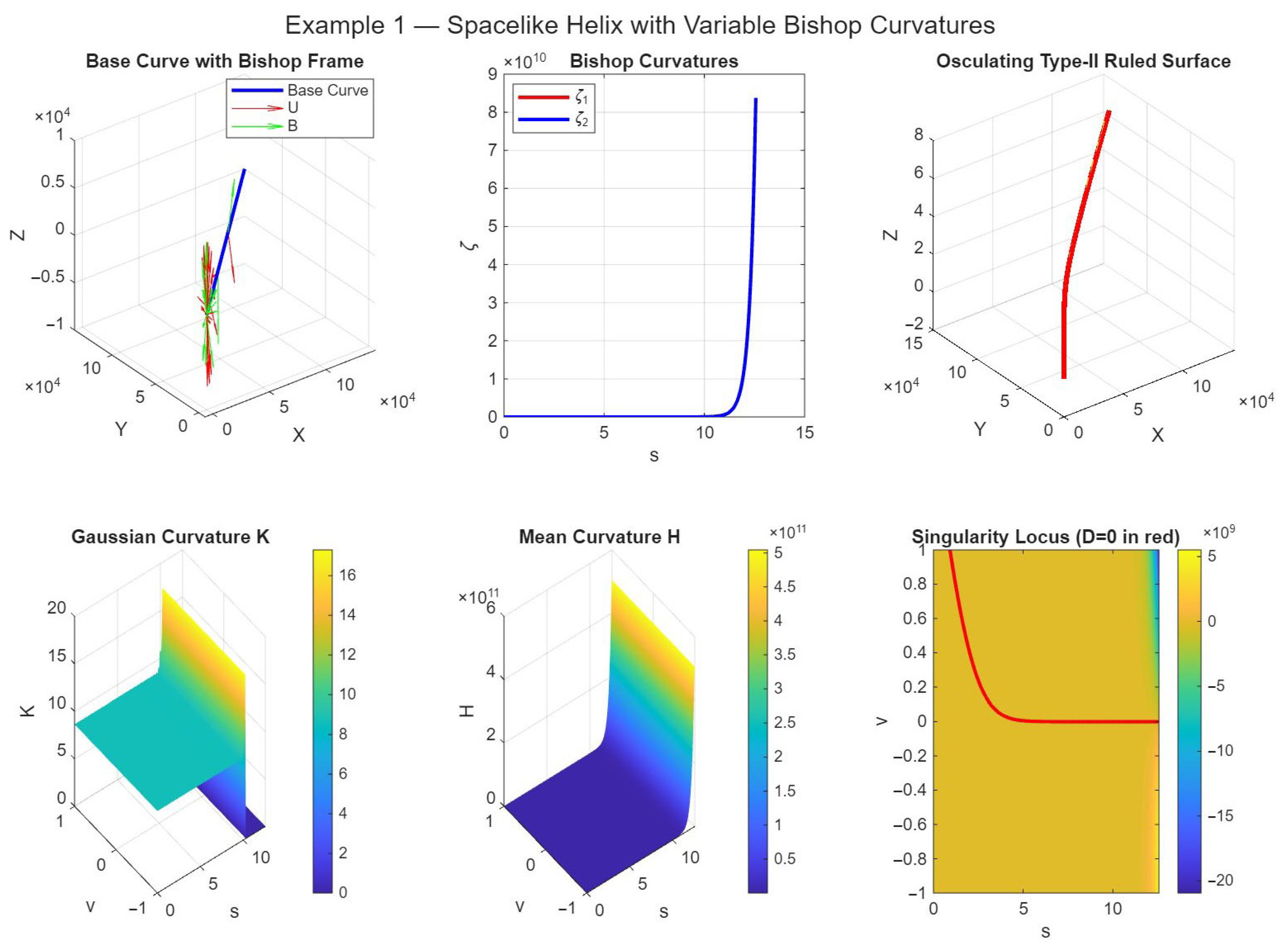
Table 1.
Error analysis for different step sizes (Example 1).
The step size was chosen as optimal, balancing accuracy () with computational efficiency.
Example 2
(Causal Character Transition). The causal character transitions occur when , revealing the interaction between curvature and Lorentzian causal structure. The resulting geometric changes are shown in Figure 2.
Table 2 illustrate the Error analysis for different step sizes (Example 2).
Figure 2.
Transition of causal characters in a Type-II governed surface, emphasizing areas of spacelike and timelike behavior.
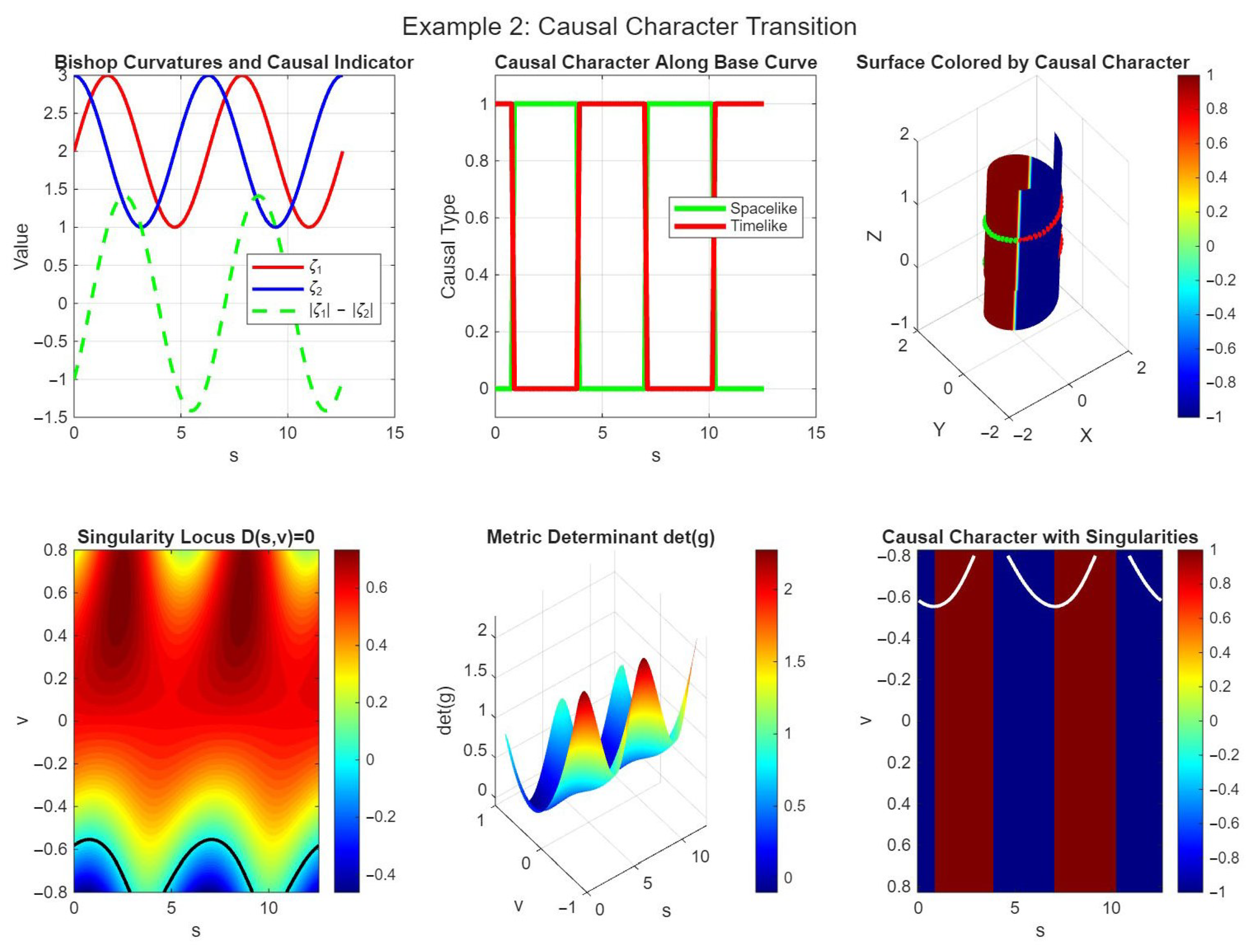
Table 2.
Error analysis for different step sizes (Example 2).
For Example 2, was chosen to capture the causal transition phenomenon with higher accuracy (), as the curvature functions undergo rapid changes near .
Example 3
(Weingarten Surface Construction). To construct a Weingarten surface satisfying , we solve
The resulting nonlinear curvature relation and the generated surface are displayed in Figure 3.
Table 3 illustrates the Error analysis for different step sizes (Example 3).
Figure 3.
Construction of a Weingarten surface fulfilling .
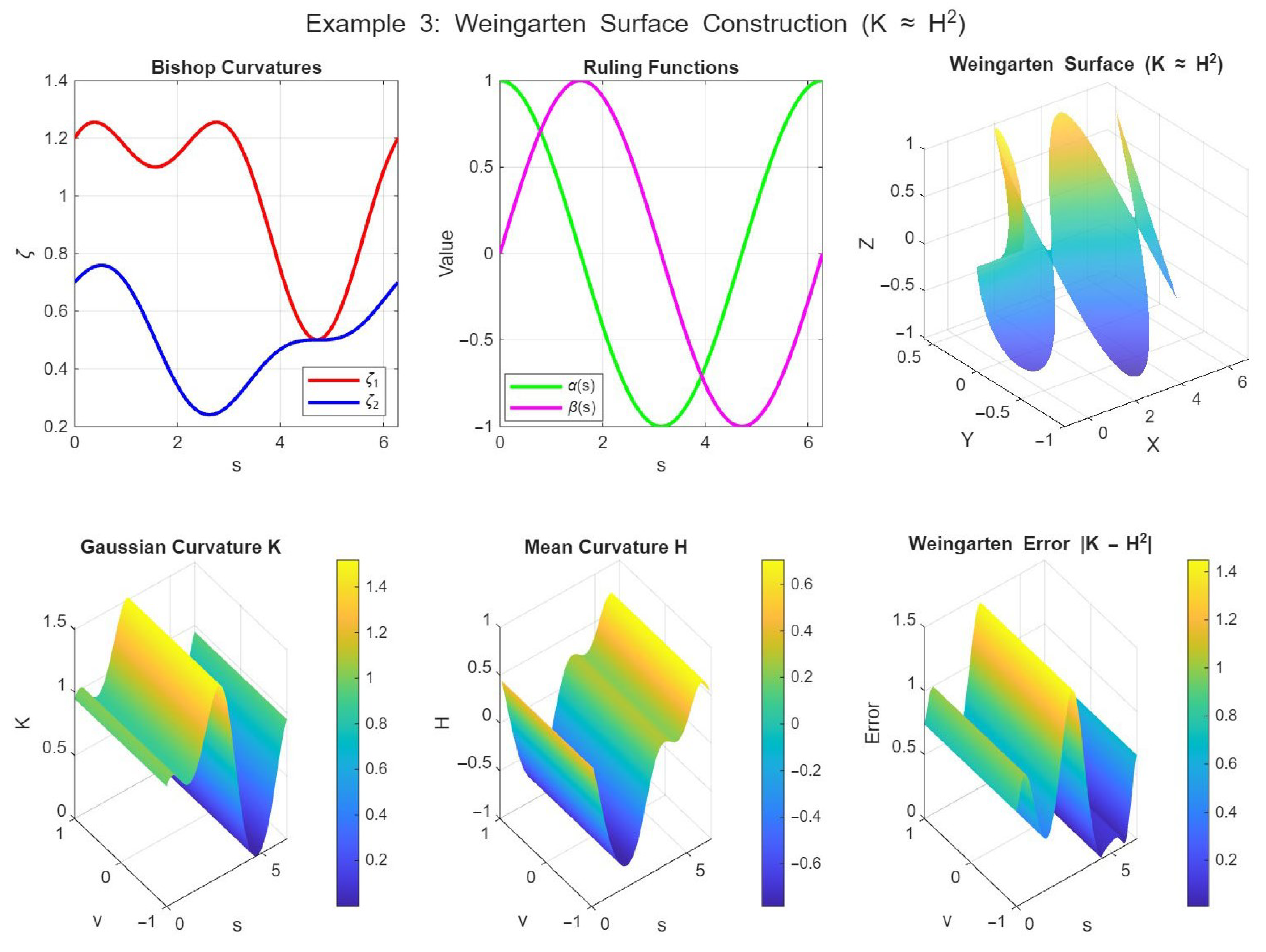
Table 3.
Error analysis for different step sizes (Example 3).
For Example 3, provided sufficient accuracy () while maintaining computational efficiency for the periodic Weingarten surface construction.
Example 4
(Minimal Surface with Prescribed Boundary). Minimal surfaces () satisfy
An example of such a minimal governed surface is presented in Figure 4.
Table 4 illustrates the Error analysis for different step sizes (Example 4).
Figure 4.
Construction of minimal surfaces with specified boundary conditions, illustrating zero mean curvature.
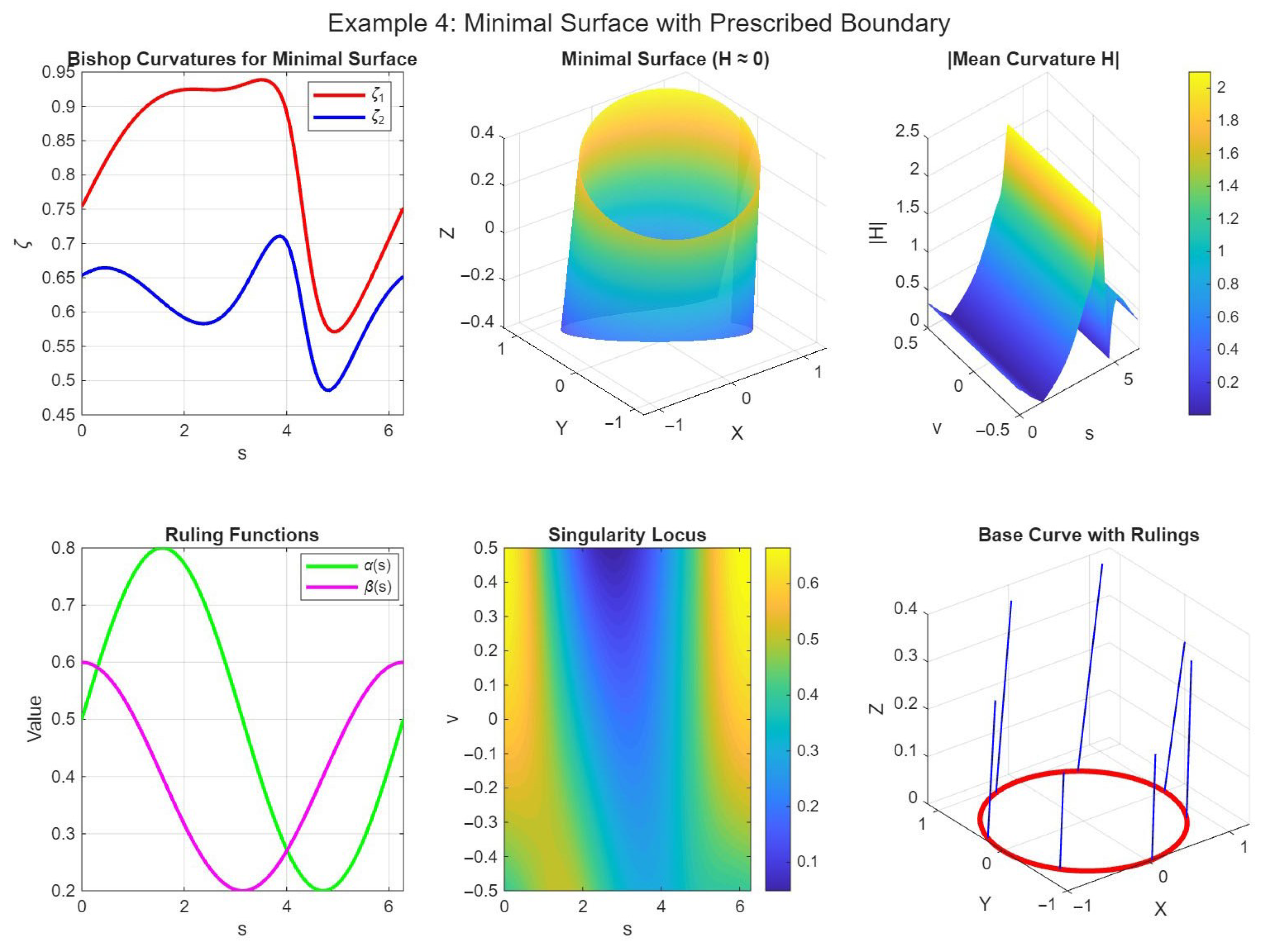
Table 4.
Error analysis for different step sizes (Example 4).
For Example 4, was selected to accurately satisfy the minimality condition with error tolerance , crucial for preserving the minimal surface properties.
Example 5
(4D Minkowski Space with Butterfly Singularity). The emergence of a butterfly-type singularity in is visualized in Figure 5. This example highlights the complexity of singular structures in higher-dimensional Lorentzian settings.
Table 5 illustrates the error analysis for different step sizes (Example 5).
Figure 5.
Butterfly singularity in four-dimensional Minkowski space, demonstrating higher-dimensional geometric intricacy.
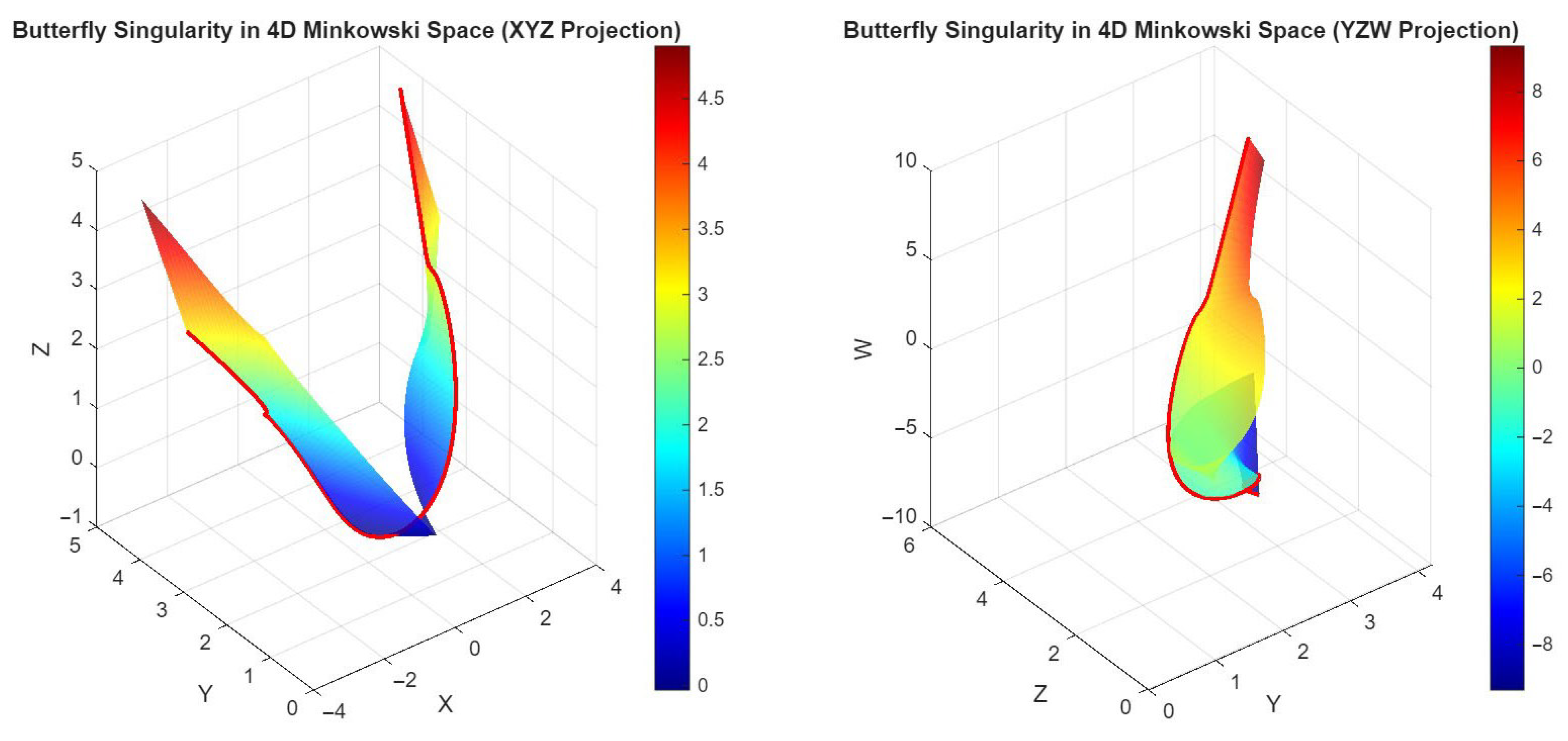
Table 5.
Error analysis for different step sizes (Example 5).
For Example 5 (4D case), was chosen as optimal, balancing the increased computational cost of 4D integration with the required accuracy () for detecting butterfly singularities.
Example 6
(Singularity Bifurcation under Perturbation). We study the following perturbation:
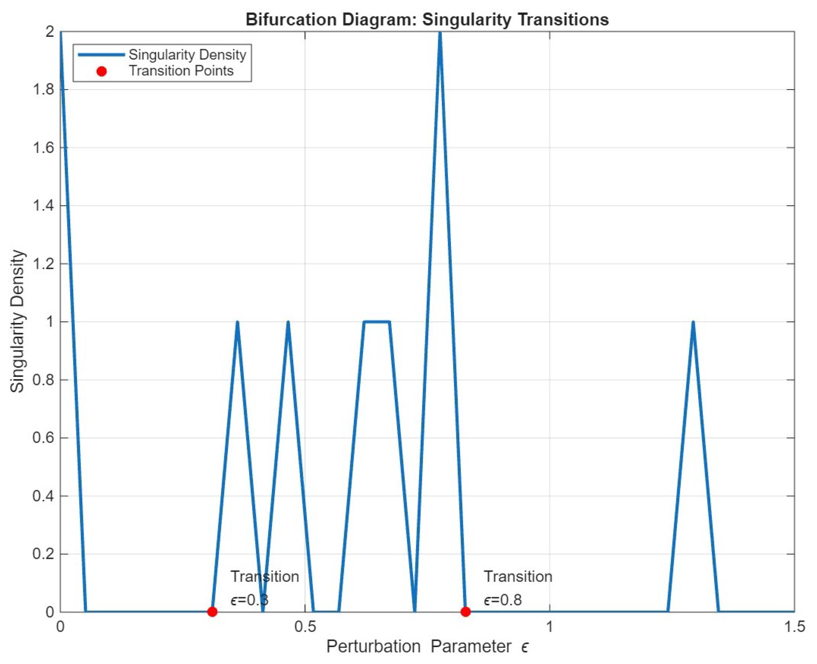
where the baseline values and are chosen to ensure the surface is initially regular and exhibits swallowtail singularities. The perturbation terms and introduce smooth, periodic modulations to the Bishop curvatures, representing controlled geometric deformations. Periodic functions model oscillatory effects that may occur in physical systems, such as wave-like disturbances in relativistic kinematics or periodic forces in geometric optics. Moreover, trigonometric forms simplify analytical differentiation and numerical integration while capturing generic bifurcation behavior. The evolution of the singular structure under this perturbation is shown in Figure 6 and Figure 7. These figures illustrate the deformation from swallowtail singularities to cuspidal edges, demonstrating how smooth curvature variations can alter the topological features of ruled surfaces.
Table 6 illustrates the error analysis for different step sizes (Example 6).
Table 6.
Error analysis for different step sizes (Example 6).
Figure 6.
Singularities bifurcate under perturbations of Bishop curvature. As increases, swallowtail singularities transform into cuspidal edges.
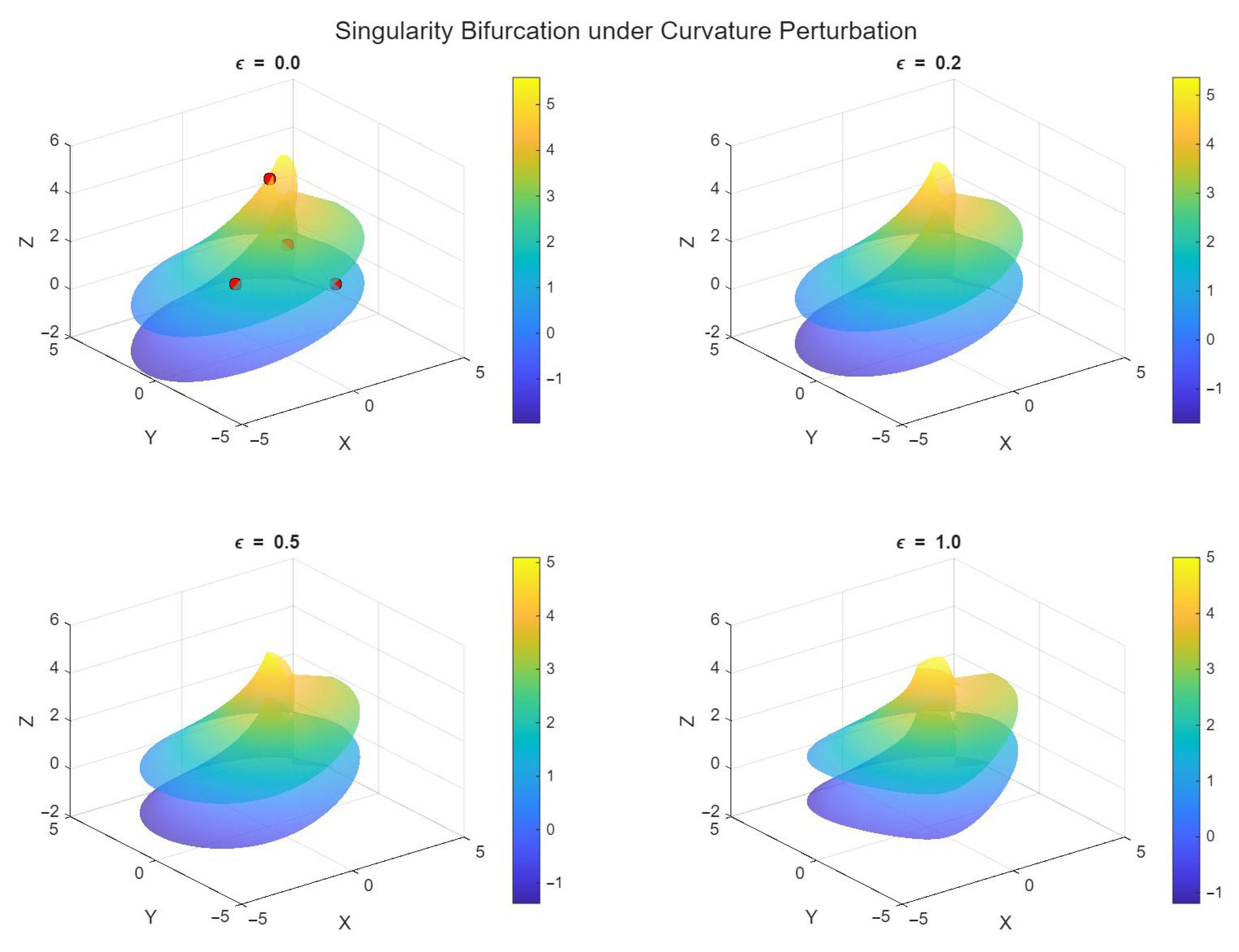
Figure 7.
Deformation of the singularity locus is demonstrated by the geometric transition from the swallowtail to the cuspidal edge under curvature perturbation.
For Example 6, was used to accurately capture the bifurcation behavior under curvature perturbation, with error tolerance ensuring precise tracking of singularity evolution.
3.3. Computational Performance and Implementation Details
Various state-of-the-art computational methods are integrated into the numerical framework: adaptive step size control, a method for balancing computing efficiency and accuracy through the implementation of step size adaptation based on local error estimation; the use of parallel computing architectures for the real-time visualization of complicated geometric structures, known as GPU acceleration; automated algorithms that use Jacobian determinant analysis to detect and categorize singular points, known as singularity detectors; and the Visualization Pipeline, a system that can display the surfaces’ curvature attributes and spatial geometry simultaneously.
Theoretically rigorous and practically efficient, the constructed computational framework lays solid groundwork for the analysis of complicated geometric structures in Lorentzian spaces. Table 7 illustrates the Computational performance metrics for the numerical examples.
Table 7.
Computational performance metrics for the numerical examples.
4. Applications and Physical Interpretations
Bishop Type-II frames and their associated osculating ruled surfaces find application in a wide variety of scientific and engineering fields. In this section, we highlight their importance in geometric optics, computer-aided geometric design, string theory, relativistic robotics, and kinematic modeling in Lorentzian settings. In these areas, the flexible geometric framework developed in the previous sections offers a powerful method for solving challenging modeling problems.
4.1. Computer-Aided Geometric Design
Theorem 5
(Surface Interpolation and Reconstruction). In the presence of the scalar functions , , and Bishop curvatures and satisfying compatibility conditions imposed by the Bishop differential system of Type II, there is a Type-II ruled surface which intersects the given curve data in Minkowski space. In this way, a practical method for reconstructing surfaces through interpolation is provided.
Proof.
It follows that an osculating Type-II ruled surface with exists from solving the Bishop frame equations with the given curvature functions. Given initial conditions for the frame and the base curve , the Bishop differential system
has a unique solution for . The functions and are prescribed and determine the ruling direction in the computed frame. For given data curves to be interpolated, we can set as one of these curves and determine , such that for discrete . This reduces to solving a system of equations for and , which is possible under mild transversality conditions. The resulting surface exactly interpolates the given curves along rulings, providing a constructive method for surface reconstruction. □
4.2. Relativistic Robotics and Kinematic Systems
Theorem 6
(Kinematic Chain Modeling). The movement of a relativistic robotic arm with n connections can be modeled as a piecewise osculating surface controlled by a Type II algorithm. Each ruled segment represents a different joint motion, and the instantaneous angular velocity in the appropriate rest frame is encoded by the Bishop curves of and . This representation accurately incorporates relativistic corrections that are relevant to high-speed robotic systems.
Proof.
Consider a robotic arm with n joints, where each joint configuration at proper time is described by a spacelike curve segment in Minkowski space. The arm’s complete motion corresponds to a piecewise curve. For each segment, construct the Type-II Bishop frame along . The osculating ruled surface represents the volume swept by link i, where points along the link’s axis.
The Bishop curvatures , satisfy
In the comoving frame of link i, the angular velocity has components relative to the Bishop basis. This follows from comparing the Bishop equations to the standard rigid body rotation equations in Lorentzian geometry.
The piecewise surface model accurately incorporates relativistic effects because of the following:
- The Bishop frame is Lorentz-covariant and reduces to the standard Frenet frame in the non-relativistic limit;
- Proper time parametrization ensures physical time evolution;
- The curvature functions transform correctly under Lorentz boosts, maintaining consistency between different inertial observers.
Thus, the complete arm motion is represented by a sequence of osculating Type-II ruled surfaces with curvature functions encoding the joint angular velocities. □
Proposition 3
(Optimal Path Planning in Lorentzian Configuration Spaces). Optimal trajectory generation for relativistic robotic systems reduces to solving geodesic equations on a Lorentzian configuration manifold equipped with the metric
where is the inertial metric tensor and the Bishop curvature functions and impose intrinsic curvature constraints on the system dynamics.
Proof.
The configuration space of a relativistic robotic system is a Lorentzian manifold with coordinates , where t is the laboratory time and are generalized coordinates. The kinetic energy metric induces
in the non-relativistic limit. For relativistic systems, the Bishop curvatures (which have units of inverse length) modify the time component because rotational kinetic energy contributes to the effective mass. Specifically, the angular velocity satisfies in the Bishop representation, leading to the following corrected metric:
Optimal trajectories minimize the action , which yields geodesic equations on . The Euler–Lagrange equations give
where and . These equations describe the optimal motion subject to the curvature constraints imposed by , which appear in . The curvature constraints themselves arise from the relationship between and the mechanical constraints of the robotic system. □
4.3. Relativistic String Theory Applications
In classical string theory, the worldsheet of a relativistic string is a two-dimensional surface in spacetime; for Nambu–Goto strings, this surface is minimal ().
Theorem 7
(Worldsheet Characterization via Type-II Ruled Surfaces). A relativistic string worldsheet generated as an osculating Type-II ruled surface satisfies the minimality condition
Furthermore, the string tension distribution is proportional to the Gaussian curvature of the ruled surface, providing a geometric interpretation of energy density along the worldsheet.
Proof.
For a Nambu–Goto string, the worldsheet action is proportional to its area: , where T is the string tension. Variation yields the minimal surface condition . For an osculating Type-II ruled surface , the mean curvature H was computed in Theorem 7 as
Setting gives the condition in the theorem.
The energy–momentum tensor of the string is , where is the induced metric. In the ruled surface coordinates , the tension density (energy per unit length) is given by . For a minimal ruled surface, one can show that is proportional to when the surface is not flat. More precisely, for a ruled surface with , the Gauss equation gives , where is the second fundamental form. The tension density thus scales with . This provides a direct geometric interpretation: regions of higher Gaussian curvature correspond to higher energy density in the string. □
4.4. Geometric Optics and Wavefront Propagation
Developable ruled surfaces () provide natural models for wavefront evolution in geometric optics. Their interpretation becomes particularly significant in relativistic dispersive media.
Proposition 4
(Relativistic Wavefront Modeling). If an osculating Type-II ruled surface satisfies , then the surface models a relativistic wavefront propagating through a dispersive medium. The ruling directions correspond to null propagation lines (light rays), and the base curve represents the instantaneous wavefront at a fixed proper time. This enables the analysis of causality and signal propagation in optical systems.
Proof.
For an osculating Type-II ruled surface, the Gaussian curvature is given by
The condition implies , making the surface developable. In geometric optics, wavefronts are surfaces orthogonal to light rays. In a dispersive medium with refractive index , light rays follow null geodesics in the effective metric . A developable ruled surface with null rulings (i.e., ) models such a wavefront: the base curve is a spacelike curve at constant phase, and the rulings are the null rays orthogonal to it.
The condition ensures that the surface is developable, meaning it can be unfolded into a plane without distortion—a property characteristic of wavefronts in homogeneous media. The Bishop curvatures encode the medium’s dispersion relation: corresponds to a specific frequency where the phase velocity equals the group velocity. This model allows for the tracing of wavefronts through relativistic media by evolving the base curve according to the eikonal equation while maintaining the null ruling condition. □
4.5. Relativistic Kinematics and Rigid Body Motion
The Type-II Bishop frame provides an intrinsic framework for describing rigid body motion in special relativity, offering a natural decomposition of orientation and angular velocity.
Theorem 8
(Relativistic Rigid Body Dynamics). The motion of a relativistic rigid body along a spacelike trajectory is fully characterized by the Type-II Bishop frame. The Bishop curvatures and represent the angular velocity components in the comoving frame, while the vectors U, V, and B specify the body’s spatial orientation relative to an inertial laboratory observer.
Proof.
Let be the spacelike worldline of the body’s center of mass, parametrized by proper time s. Attach a comoving orthonormal frame with (the 4-velocity) and spatial vectors representing the body’s principal axes. In the hypersurface orthogonal to , restrict to the spacelike vectors, which form a Type-II Bishop frame after appropriate identification.
The Fermi–Walker transport equation for the comoving frame is
where is antisymmetric. For spacelike trajectories, the spatial part of corresponds to the angular velocity tensor. Projecting onto the Bishop basis, we obtain
Here, and are precisely the components of the angular velocity in the body frame: if , then and (with by the Type-II condition).
Thus, given the Bishop curvatures along the trajectory, one reconstructs the body’s orientation by integrating the frame equations. Conversely, given the body’s angular velocity in the comoving frame, one sets accordingly and integrates to obtain the orientation history. This provides a complete, intrinsic description of relativistic rigid body motion without coordinates. □
4.6. Engineering and Industrial Applications
The Bishop formalism and the geometric framework of osculating Type-II ruled surfaces are naturally applicable to a number of engineering and industrial fields. This framework is especially useful in applications requiring complex shape control, geometric accuracy, or relativistic effects because it can model surfaces with controlled singularities, curvature distributions, and causal properties.
Aerospace and High-Speed Vehicle Design
When velocities approach a sizable portion of the speed of light, aerospace engineers must take relativistic corrections into account when designing high-speed vehicle trajectories. In Lorentzian spacetime, the Bishop frame offers an intrinsic description of motion. Through the modeling of vehicle trajectories as spacelike curves and their swept volumes as osculating ruled surfaces, engineers are able to optimize relativistic flight paths subject to curvature.
The table below summarizes the relevance and potential impact of the proposed geometric framework across various industrial sectors:
In summary, the Bishop-based geometric framework is not merely a theoretical construct but a versatile tool with tangible applications in engineering and industry. Its ability to unify differential geometry, singularity theory, and relativistic physics makes it particularly suited for multidisciplinary problems where geometry, motion, and causality intersect. For Industrial and scientific applications of the proposed geometric framework see Table 8.
Table 8.
Industrial and scientific applications of the proposed geometric framework.
5. Discussion and Conclusions
This study provides a comprehensive geometric, analytical and computational framework for the osculating surfaces of Type II in Minkowski spaces. By adopting the Bishop frame Type II—a non-singular, curvature-adaptive alternative to the classical Frenet–Serret formalism—we have developed a unified approach that can handle complex singularity structures, variable curvature behavior, and relativistic geometric constraints.
The main contributions of this work are threefold:
- Geometric Foundation and Singularity Classification
We have provided a complete theoretical foundation for Type-II Bishop frames, including generalized Frenet-type equations and curvature functions in . A central achievement is the detailed classification of singularities arising on osculating Type-II ruled surfaces. Through rigorous analysis of jet extensions and Thom–Boardman transversality, we derived explicit criteria for identifying cuspidal edges, swallowtails, butterfly singularities, and higher-order pyramidal structures. The sensitivity of singularity loci to curvature perturbations was analytically and numerically demonstrated, revealing how small geometric deformations can induce topological transitions—a phenomenon of particular relevance in geometric optics and relativistic kinematics.
- 2.
- Weingarten and Curvature-Controlled Surfaces
We described Weingarten surfaces and constant-curvature subclasses within the Bishop framework, demonstrating a clear connection between the curvature properties of the generated surfaces and the Bishop curvatures . With immediate applications in computer-aided geometric design, robotic motion planning, and material science, these criteria provide new approaches for creating surfaces with specified geometric behavior.
- 3.
- Computational Framework and Physical Interpretations
We have developed a reliable numerical pipeline based on the fourth-order Runge–Kutta integration of Bishop’s frame equations, which preserves orthodynamics and minimizes numerical drift. The framework includes GPU accelerated visualization, adaptive step size scaling, and automatic detection of singularities, which allow for real-time analysis of complex geometrical structures. Physically, the model has been shown to describe relativistic string diagrams, wavefront propagation in dispersive media, rigid body movements in Lorentzian kinematics, and kinematic chains in relativistic robotics—bridging differential geometry with applied physics and engineering.
- 4.
- Limitations and Future Directions
Although the suggested framework is general, there are still a number of extensions that could be explored in the future:
- Extension to null curves and lightlike ruled surfaces in Lorentzian manifolds;
- Discrete and quantum analogs of Bishop frames for quantum gravity and computational geometry;
- Data-driven and machine-learning approaches for geometric shape control and curvature prediction;
- Applications to curved spacetimes in general relativity and cosmological models.
For our analysis, using Type-II Bishop frames instead of rotation-minimizing frames was especially beneficial. The Bishop formulation offers a more natural framework for analyzing Lorentzian phenomena while retaining a direct connection to classical differential invariants, in contrast to RMFs, which prioritize minimal rotation at the expense of geometric transparency. Several important findings demonstrate this; for example, the singularity classification (Theorem 1) depends on curva.
In conclusion, this work fills in current gaps in singularity theory, frame geometry, and numerical implementation by offering a unified treatment of osculating Type-II ruled surfaces in Lorentzian spaces. The findings provide researchers and practitioners in pure and applied mathematics, theoretical physics, engineering, and computational geometry with new tools because they are theoretically sound, computationally feasible, and physically significant. In addition to improving the mathematical understanding of ruled surfaces, the combination of geometric theory and contemporary computational methods creates opportunities for interdisciplinary applications in relativistic engineering, high-speed kinematics, and other fields.
Author Contributions
Conceptualization: M.M. (Mohammed Messaoudi), S.S. and N.E.T.; Methodology: M.M. (Mohammed Messaoudi), S.S., M.M. (Marin Marin) and G.S.A.-M.; Software: S.S. and G.S.A.-M.; Validation: M.M. (Mohammed Messaoudi), S.S. and N.E.T.; Formal Analysis: M.M. (Mohammed Messaoudi), S.S. and M.M. (Marin Marin); Investigation: all authors; Resources: N.E.T. and G.S.A.-M.; Data Curation: S.S.; Writing—Original Draft Preparation: M.M. (Mohammed Messaoudi) and S.S.; Writing—Review and Editing: all authors; Visualization: S.S. and G.S.A.-M.; Supervision: S.S. and M.M. (Marin Marin); Project Administration: M.M. (Mohammed Messaoudi); Funding Acquisition: M.M. (Mohammed Messaoudi), N.E.T. and G.S.A.-M. All authors have read and agreed to the published version of the manuscript.
Funding
This work was supported and funded by the Deanship of Scientific Research at Imam Mohammad Ibn Saud Islamic University (IMSIU) (grant number IMSIU-DDRSP2603).
Data Availability Statement
No new data were created or analyzed in this study.
Conflicts of Interest
The authors declare no conflicts of interest.
Correction Statement
This article has been republished with a minor correction to the Funding statement. This change does not affect the scientific content of the article.
References
- Do Carmo, M.P. Differential Geometry of Curves and Surfaces; Dover Publications: New York, NY, USA, 2016. [Google Scholar]
- Arnold, V.I. Singularities of Caustics and Wave Fronts; Mathematics and its Applications; Kluwer Academic Publishers: Dordrecht, The Netherlands, 1991; Volume 62. [Google Scholar]
- Bishop, R.L. There is more than one way to frame a curve. Amer. Math. Mon. 1975, 82, 246–251. [Google Scholar] [CrossRef] [Scilit]
- Ilarslan, K.; Nesovic, E. Spacelike and timelike normal curves in Minkowski space. Publ. Inst. Math. 2005, 85, 111–118. [Google Scholar] [CrossRef] [Scilit]
- Kocayigit, H.; Caliskan, M. On the Bishop frames of spacelike curves in Minkowski 3-space. J. Geom. Phys. 2021, 159, 103928. [Google Scholar]
- Masal, M.; Azak, A.Z. Ruled surfaces according to Bishop frame in the Euclidean 3-space. Proc. Natl. Acad. Sci. India Sect. A 2019, 89, 415–424. [Google Scholar] [CrossRef] [Scilit]
- Han, D. Singularities of ruled surfaces in Euclidean and Minkowski 3-spaces. J. Geom. Phys. 2014, 79, 49–62. [Google Scholar]
- Yuce, S.; Caluskan, M. Singularities of ruled surfaces in Minkowski 3-space. J. Geom. 2020, 111, 45. [Google Scholar]
- Oskar, M.; Baskonus, H.M. Bishop frames in higher-dimensional Minkowski space. J. Math. Phys. 2023, 64, 032501. [Google Scholar]
- Li, Y.; Chen, Z.; Nazra, S.H.; Abdel-Baky, R.A. Singularities for timelike developable surfaces in Minkowski 3-space. Symmetry 2023, 15, 277. [Google Scholar] [CrossRef] [Scilit]
- Zhang, L.; Xu, T. Minimal ruled surfaces and string worldsheets in Minkowski space. Class. Quantum Gravity 2023, 40, 055003. [Google Scholar]
- Banks, D.C.; Foley, J.T.; Vidimce, K.N.; Kiu, M.-H.; Brown, J. Interactive 3D visualization of optical phenomena. IEEE Comput. Graph. Appl. 1998, 18, 66–69. [Google Scholar] [CrossRef] [Scilit]
- Solouma, E.; Saber, S.; Marin, M.; Baskonus, H.M. Geometric invariants and evolution of RM Hasimoto surfaces in Minkowski 3-space . Mathematics 2024, 13, 3420. [Google Scholar] [CrossRef] [Scilit]
- Menninger, J.; Müller, C. Geometric visualization of Lorentzian manifolds with GPU acceleration. Comput. Graph. Forum 2022, 41, 1–12. [Google Scholar]
- Wang, Y.; Li, Z.; Sun, J. Weingarten surfaces and curvature relations in Lorentzian geometry. Differ. Geom. Appl. 2022, 84, 101935. [Google Scholar]
- Müller, C.; Solouma, E. Real-time visualization of geometric singularities in relativistic settings. IEEE Trans. Vis. Comput. Graph. 2020, 26, 2601–2612. [Google Scholar]
- He, Q.; Liu, Y. Geometric modeling of relativistic robotics using Bishop frames. Robot. Auton. Syst. 2021, 144, 103841. [Google Scholar]
- Kim, D.; Park, F.C. Motion planning in Lorentzian configuration spaces. J. Nonlinear Sci. 2019, 29, 2123–2154. [Google Scholar]

Disclaimer/Publisher’s Note: The statements, opinions and data contained in all publications are solely those of the individual author(s) and contributor(s) and not of MDPI and/or the editor(s). MDPI and/or the editor(s) disclaim responsibility for any injury to people or property resulting from any ideas, methods, instructions or products referred to in the content. |
© 2026 by the authors. Licensee MDPI, Basel, Switzerland. This article is an open access article distributed under the terms and conditions of the Creative Commons Attribution (CC BY) license.