Tau-Theory-Based Guidance Methodology for Helicopter Obstacle Field Navigation ^†

Abstract

This study presents a Tau-theory-based guidance methodology for obstacle avoidance in low-altitude, high-speed rotorcraft operations, especially within obstacle-dense and degraded visual environments (DVEs). A geometric approach is employed to develop the obstacle avoidance algorithms. The methodology considers both inner-loop and outer-loop guidance with a decision logic that determines the appropriate maneuver (turn, climb, or deceleration) based on real-time analysis of the environment and the helicopter’s operational limits. Extensive desktop simulations conducted in the MATLAB/Simulink environment, using FLIGHTLAB^® high-fidelity nonlinear models and different pilot models, demonstrate the method’s ability to guide pilots with safe and efficient trajectories for obstacle field navigation. These findings lay the groundwork for potential real-world implementations in both manned and autonomous rotorcraft missions.

1. Introduction

Operating a helicopter close to the terrain with low situational awareness (SA) significantly increases risk by dramatically reducing reaction times. The Tau-theory-based obstacle avoidance methodology aims to facilitate real-time trajectory adjustments through visual cueing applications or autopilot implementations. This methodology focuses on reducing workload and improving pilot SA without increasing cognitive load while maneuvering around obstacles in obstacle-dense and degraded visual environments. The goal of this methodology is to enhance the safety and efficiency of low-altitude, high-speed rotorcraft missions.

The Tau-theory-based obstacle avoidance methodology comprises either the inner-loop guidance algorithms, consisting of bank angle guidance, rate of climb guidance, and pitch angle guidance, or the outer-loop guidance algorithms, consisting of heading angle guidance, flight path angle guidance, and deceleration trajectory guidance. They correspond to three obstacle avoidance maneuvers: turning away from the obstacle, climbing over the obstacle, and reducing speed for successful obstacle field navigation. Decision logic integrates these algorithms, ensuring smooth transitions between them across varying obstacle fields.

In this study, several desktop simulations were performed in the MATLAB/Simulink (v24a) environment during the development phase using pilot models. These simulations served both as sensitivity analysis to determine key design parameters and as evaluations of system performance.

The main novelty of the proposed Tau-theory-based guidance methodology lies in its ability to operate in real-time without any prior knowledge of the surrounding environment. The algorithm provides three-dimensional obstacle avoidance guidance in generic and dynamically changing environments, remaining independent of the number, size, or geometric complexity of the obstacles encountered. Because the approach is formulated entirely through simple geometric relations, it is computationally efficient and well suited for real-time onboard implementation. Its modular structure also enables straightforward integration with different sensing technologies—including LiDAR, radar, or vision-based systems—making it highly adaptable to a wide range of rotorcraft platforms and operational conditions. The ease of implementation and low computational demand make the method particularly advantageous for both piloted vehicles via appropriate cueing and Unmanned Aerial Vehicles (UAVs) with embedded autonomous guidance systems.

The paper is organized as follows. Introduction introduces the motivation and objectives of developing a real-time obstacle avoidance methodology for rotorcraft operating in obstacle-dense and degraded visual environments. Section 2 reviews previous research on obstacle avoidance, trajectory generation, and guidance algorithms, highlighting the limitations of existing approaches. Section 3 presents the proposed Tau-theory-based guidance methodology, describing the inner-loop and outer-loop guidance algorithms associated with turning, climbing, and deceleration maneuvers, along with the decision logic that governs transitions between them. Section 4 details the simulation setup, sensitivity analysis, and performance evaluation, comparing the inner-loop and outer-loop guidance implementations under various flight scenarios. Finally, Section 4.4 summarizes the main findings, discusses the advantages of the proposed approach in terms of real-time feasibility and adaptability, and outlines directions for future work.

2. Background

Obstacle avoidance is a widely studied problem for various types of vehicles. Over the years, several methods have been developed to address this challenge, including reactive methods based on geometry/kinematics [1,2], optimal trajectory generation [3], path planning based on the panel method [4], pilot cueing [5], and others [6,7,8,9,10,11].

Recent research further extends these developments with a wide range of modern obstacle-avoidance strategies, including bio-inspired and hybrid optimization-based trajectory planning [12,13,14], reactive potential-field and safety-field approaches incorporating improved repulsion dynamics and stability considerations [15,16,17,18], sampling-based local replanning integrated with real-time perception and mapping [19,20], geometric clustering and environment-understanding techniques using LiDAR–camera fusion or Gaussian-mixture modeling [21,22], heuristic trajectory generation for complex infrastructure inspections [23], maneuver-primitive/trim-library-driven agile guidance for fixed-wing UAVs [24], and multi-agent or learning-based approaches enabling cooperative and adaptive avoidance behavior in dynamic environments [25,26,27].

Many studies have aimed to improve the ability to detect and avoid obstacles safely and efficiently. Although these studies have achieved significant progress, most still rely on predefined environment data, heavy computation, or simplified vehicle dynamics. The goal of the proposed Tau-theory-based guidance method is to overcome these issues by using time-to-collision information as a perceptual variable, enabling real-time, map-independent obstacle avoidance within realistic helicopter performance limits.

Binet and Rakotomamonjy [5] developed an obstacle avoidance methodology for a helicopter using Tau theory [28], introducing haptic cueing through force bias on the lateral cyclic. Building upon this approach, a visual guidance method based on Tau theory was proposed in [29]. This method generates bank angle guidance to help the pilot execute a coordinated turn, avoiding obstacles and safely adjusting the helicopter’s trajectory. The rotorcraft’s altitude and speed are maintained throughout the maneuver, while obstacles are treated as having infinite height, limiting the method to the two-dimensional (2D) plane. Consequently, further adjustments were required to extend the methodology to a three-dimensional (3D) space.

Padfield [30] explains that when pilots encounter obstacles, they have three options: turn away, climb over, or stop before reaching the obstacle. Stopping is the least favorable option for time-critical missions as it risks compromising mission success. Therefore, pilots may be advised to decelerate if the helicopter’s operational limits are exceeded during a turning or climbing maneuver. In light of these considerations, Esmek et al. [31] propose an algorithm incorporating three guidance methods—bank angle guidance, rate of climb guidance, and pitch angle guidance—along with a decision logic to ensure smooth transitions between them. Although bank angle guidance addresses 2D obstacle avoidance, the rate of climb guidance extends the capability to 3D space. Deceleration guidance further enhances safety and, with decision logic, the algorithm operates seamlessly under varying terrain and flight conditions.

Tau theory [28] forms the foundation for the algorithms that generate the bank angle, the rate of climb, and the deceleration guidance. The deceleration guidance algorithm calculates the deceleration trajectory while maintaining a constant rate of change of $\tau$, following Lee’s study [28] on how time-to-collision information influences visual control of braking in traffic. Once the deceleration trajectory is generated, it is converted into pitch angle guidance through dynamic inversion (DI), as described in [32]. Finally, the decision logic ensures smooth transitions between guidance methods based on desktop simulations that assess the individual performance of the bank angle and rate of climb guidance algorithms. This approach ensures that the helicopter remains within its operational limits while safely navigating around obstacles.

Although the inner-loop guidance presented in [31], which includes bank angle, pitch angle, and rate of climb guidance, performs well in desktop simulations using a pilot model, pilot interviews indicate that it is highly time-sensitive, leaving pilots with almost no reaction time. This increases the workload and necessitates an outer-loop guidance. To address this, Esmek et al. [33] consider outer-loop guidance in addition to making the decision logic used in [31] more elaborate by accounting for power and rotor stall limits.

3. Methodology

Inner-loop and outer-loop guidance methodologies associated with three obstacle avoidance maneuvers, i.e., turning, climbing, and deceleration, are explained in the following sections.

Table 1. Guidance methods.

Maneuver	Inner-Loop	Outer-Loop
Turn	Bank Angle	Heading Angle
Decelerate	Pitch Angle	Deceleration Trajectory
Climb	Rate of Climb	Flight Path Angle

summarizes the guidance methods. The inner-loop guidance generates attitude-level guidance for immediate obstacle avoidance, while the outer-loop guidance provides trajectory adjustments. The decision logic determines which avoidance maneuver should be executed and when it should begin.

3.1. Inner Loop Guidance

The inner-loop guidance consists of bank angle guidance for turning, rate of climb guidance for climbing, and pitch angle guidance for deceleration.

3.1.1. Bank Angle Guidance

The geometric approach of the bank angle guidance algorithm is illustrated in Figure 1. In this algorithm, an obstacle of any shape is surrounded by a red circle with radius $R_O$ with center O. A safety bubble outside the obstacle is shown as a green circle with a radius of $R_S$. $R_S$ is one of the design parameters whose value can be set via extensive simulations for successful avoidance. The helicopter is also inside a black circle with a radius of $R_H$ with a center of C, which is the helicopter’s center of gravity.

The pilot is expected to perform a turn maneuver to follow the brown line (dash-dot-dash line) shown in Figure 1. This algorithm calculates the necessary bank angle ($\phi$) guidance to complete this turn maneuver. The goal is to clear the obstacle by making a coordinated turn until the ground velocity, which can be seen as the orange solid arrow as ${\overrightarrow{V_G}}^I$ in Figure 1, and the tangent line between the helicopter and the safety bubble are parallel to each other. In this algorithm, an Inertial Reference Frame fixed to Earth is used. The superscript and subscript “I” represent the Inertial Reference Frame. The $x_I$-axis of the inertial frame points to the North, the $y_I$-axis to the East, and the $z_I$-axis down.

Three angle definitions are used to build this algorithm. One is $\chi$, the heading angle, which indicates the direction of the helicopter’s ground speed. The ground velocity does not include the vertical velocity; it is the North-East plane projection of the vehicle’s inertial velocity. Next is $\kappa$, which is the argument of the vector drawn from the helicopter’s center of gravity to the center of the obstacle in the inertial frame. The relation for $\kappa$ angle is given in Equations (1) and (2). $\chi$ and $\kappa$ are shown in Figure 1b. The other is $\delta$, which is half the angle between the two intersecting tangent lines, as shown in Figure 1a. $\delta$ is calculated as follows:

$$C{O}_I^I=\left[\begin{array}{c}{x}_I\\ y_I\\ z_I\end{array}\right]$$

(1)

$$\kappa ={tan}^{-1}\left({\displaystyle \frac{y_I}{x_I}}\right)$$

(2)

$$\delta ={sin}^{-1}\left({\displaystyle \frac{\sqrt{R_S^2+R_H^2}}{\sqrt{x_I^2+y_I^2}}}\right)$$

(3)

The location of the obstacle with respect to the helicopter’s trajectory is determined by the relationship between $\chi$, $\kappa$, and $\delta$; in other words, three-angle information is utilized to decide whether there is a collision risk or not with the current ground velocity (${\overrightarrow{V_G}}^I$). In addition, how much angle to turn in a certain amount of time is also calculated using these angles. In this method, the direction of the turn rate is chosen according to the smallest turn rate. If $\chi$ is between ($\kappa +\delta$) and ($\kappa -\delta$), it indicates the collision risk. A right turn guidance is initiated if $|\kappa +\delta -\chi |$ is less than $|\kappa -\delta -\chi |$.

The ratio of distance and velocity formulation [28] is used to estimate time-to-collision ($\tau$). First, the instantaneous distance-to-collision is obtained as:

$$D_{remain}=\sqrt{x_I^2+y_I^2}-R_S-R_H$$

(4)

Then, $\tau$ is computed as the ratio of $D_{remain}$ and the component of the vehicle’s ground velocity along the line-of-sight between the vehicle and the obstacle.

$$\tau ={\displaystyle \frac{D_{remain}}{|{\overrightarrow{V_G}}^I|cos(\chi -\kappa )}}$$

(5)

The required turn rate ($\omega$) is determined using the time-to-collision estimate.

$$\omega ={\displaystyle \frac{|\kappa +\delta -\chi |}{\tau }}\to \mathrm{if}\mathrm{right}\mathrm{turn}$$

(6)

$$\omega ={\displaystyle \frac{|\kappa -\delta -\chi |}{\tau }}\to \mathrm{if}\mathrm{left}\mathrm{turn}$$

(7)

The radius of turn (r) becomes:

$$r={\displaystyle \frac{|{\overrightarrow{V_G}}^I|}{\omega }}$$

(8)

The required bank angle (${\phi }_{cmd}$) for a coordinated turn is obtained as:

$${\phi }_{cmd}=\pm ta{n}^{-1}\left({\displaystyle \frac{{\overrightarrow{V_G^I}}^2}{gr}}\right)$$

(9)

where g is the acceleration due to gravity. The sign of the required bank angle in Equation (9) depends on the logic that decides the direction of the turn.

The bank angle guidance begins to be computed when the estimated time-to-collision is less than a threshold time, ${\tau }_m$ (margin value of the $\tau$), chosen according to the assumption of how far the onboard sensor can detect an obstacle. ${\tau }_m$ is the second design parameter to be selected. This threshold time can also be translated as the threshold distance. However, in this study, instead of the threshold distance, the threshold time, ${\tau }_m$, is used.

3.1.2. Rate of Climb Guidance

The illustration for the rate of climb (ROC) guidance is given in Figure 2, which is a side view of Figure 1. In 3D space, it is assumed that the helicopter is inside a sphere with radius $R_H$ and the obstacle with any shape is inside a cylinder with radius $R_O$ and height $H_O$. Figure 2 shows the side view of the cylinder outside the obstacle as a red rectangle and the safety bubble extended to the height of the obstacle as a green rectangle. The radius of the safety bubble is determined by extensive simulations, as explained in the Bank Angle Guidance section.

The rate of climb guidance is calculated from the vertical distance between the height above the terrain (HAT) of the lowest point of the sphere surrounding the helicopter and the highest point of the obstacle, which is the height of the cylinder outside the obstacle. The calculation of the rate of climb guidance is given in Equations (10) and (11).

$$\mathsf{\Delta }H=H_O-(HAT-R_H)$$

(10)

$$RO{C}_{cmd}={\displaystyle \frac{\mathsf{\Delta }H}{\tau }}$$

(11)

3.1.3. Pitch Angle Guidance for Deceleration

The study by Lee [28] investigates the effect of time-to-collision information on visual control of braking in traffic, which concludes that the easiest type of information to control braking is visually perceived time-to-collision information, rather than distance, speed, or deceleration/acceleration and that the driver maintains a safe margin value of the derivative of time-to-collision (${\dot{\tau }}_m$) while controlling braking. Therefore, the deceleration guidance algorithm, which calculates the deceleration trajectory while keeping $\dot{\tau }$ constant, is based on this study. The derivation of the deceleration trajectory is explained in detail in the appendix of [28] and in Appendix A. of this manuscript. Denoting $U\left(t\right)=|{\overrightarrow{V_G}}^I\left(t\right)|cos(\chi -\kappa )$ and $X\left(t\right)=D_{remain}\left(t\right)$, Equation (5) becomes:

$$\tau ={\displaystyle \frac{X\left(t\right)}{U\left(t\right)}}$$

(12)

where $X\left(t\right)$ is the distance to the obstacle and $U\left(t\right)\ge 0$ is the magnitude of the forward speed. Therefore, as the vehicle approaches the obstacle,

$${\displaystyle \frac{dX\left(t\right)}{dt}}=-U\left(t\right)<0$$

(13)

Differentiating (12) and using (13) yields

$$\dot{\tau }={\displaystyle \frac{\dot{X}U-X\dot{U}}{U^2}}={\displaystyle \frac{(-U)U-X\dot{U}}{U^2}}=-1-\tau \left(t\right){\displaystyle \frac{1}{U\left(t\right)}}{\displaystyle \frac{dU\left(t\right)}{dt}}$$

(14)

It is assumed that the deceleration starts at $t=0$; therefore, $U\left(0\right)$ is the speed at which the deceleration starts, and $X\left(0\right)$ is the distance from the obstacle at $t=0$. The deceleration trajectory is obtained by solving (14) with the constant $\dot{\tau }={\dot{\tau }}_m$, giving the following.

$$U\left(t\right)=U\left(0\right){\left(1+{\displaystyle \frac{{\dot{\tau }}_{m}U\left(0\right)t}{X\left(0\right)}}\right)}^{-1-\frac{1}{{\dot{\tau }}_m}}$$

(15)

The deceleration trajectory Equation (15) guarantees that the vehicle stops when it reaches the obstacle, when $-1<{\dot{\tau }}_m<0$. Because deceleration occurs linearly when ${\dot{\tau }}_m=-0.5$, ${\dot{\tau }}_m$ is selected as $-0.5$ to avoid abrupt changes in the guidance.

After generating the deceleration trajectory $U\left(t\right)$, it is transformed into a pitch angle guidance using dynamic inversion as described in [32]. Figure 3 shows the block diagram of the transition from the deceleration trajectory to the pitch angle guidance. In Figure 3 u is the velocity in the x-direction of the body frame, ${\nu }_u$ is the pseudo-control, g is the acceleration due to gravity and $\theta$ is the Euler pitch angle. The stability derivative $X_u$ is scheduled with flight speed. Linear Time-Invariant (LTI) models used in the dynamic inversion are extracted at different flight speeds and zero sideslip trim conditions using the generic helicopter model in FLIGHTLAB^® v3.10.1 [34].

Since $U\left(t\right)$ is along the line-of-sight between the vehicle and the obstacle, the component of $U\left(t\right)$ along the x-axis of the body-fixed frame, $u_{cmd}$, is found as:

$$u_{cmd}=U\left(t\right)(cos\left(\kappa \right)cos\left(\psi \right)cos\left(\theta \right)+sin\left(\kappa \right)sin\left(\psi \right)cos\left(\theta \right))$$

(16)

where $\theta$ and $\psi$ are the Euler pitch and yaw angles.

A first-order command model is used to specify the desired response of the system, which is given in Equation (17), where T is the time constant. T is selected as 1 s for this application. A PI controller is used for the error compensation of the generated deceleration trajectory, where the proportional gain $K_P$ is 1 and the integral gain $K_I$ is 0.001.

$$G_{ideal}\left(s\right)={\displaystyle \frac{1}{Ts+1}}$$

(17)

An approximation to the linearized translational dynamics in the x-direction of the body frame can be written as given in [32].

$$\dot{u}=X_{u}u-g\theta$$

(18)

Replacing $\dot{u}$ with the pseudo control ${\nu }_u$ gives the required pitch angle $\mathsf{\Delta }\theta$ for deceleration guidance.

$$\mathsf{\Delta }{\theta }_{cmd}={\displaystyle \frac{X_{u}u-{\nu }_u}{g}}$$

(19)

3.2. Outer Loop Guidance

The outer-loop guidance consists of heading angle guidance for turning, flight path angle guidance for climbing, and deceleration trajectory guidance for reducing the vehicle speed.

3.2.1. Heading Angle Guidance

The heading angle guidance, ${\chi }_{cmd}$, is found using the bank angle guidance, as shown in Equation (20).

$${\chi }_{cmd}={\displaystyle \frac{tan\left({\phi }_{cmd}\right)\tau g}{|{\overrightarrow{V_G}}^I|}}$$

(20)

3.2.2. Flight Path Angle Guidance

The flight path angle guidance, ${\gamma }_{cmd}$, is found by using the rate of climb guidance, as shown in Equation (21).

$${\gamma }_{cmd}=ta{n}^{-1}\left({\displaystyle \frac{RO{C}_{cmd}}{|{\overrightarrow{V_G}}^I|cos(\chi -\kappa )}}\right)$$

(21)

3.2.3. Trajectory Guidance for Deceleration

The purpose of the deceleration trajectory guidance is to follow the commanded deceleration velocity given in Equation (16) during climbing or turning in obstacle avoidance maneuvers. It is the outer-loop form of the deceleration guidance.

3.3. Decision Logic

A decision-making algorithm is implemented to determine whether a helicopter should perform a climb or turn maneuver to avoid detected obstacles, while staying within its operational limits. The process begins by detecting all obstacles within a specified range from the helicopter’s current position. For each obstacle, the algorithm calculates its relative position and evaluates its proximity in horizontal and vertical directions.

An obstacle is considered a threat if:

• The required vertical clearance is positive (i.e., collision would occur without an obstacle avoidance maneuver)
• The obstacle lies within the collision cone,

  $$\kappa -\delta \le \chi \le \kappa +\delta$$

In this study, guidance algorithms are developed for speeds higher than 60 knots. Different guidance algorithms should be used for low-airspeed flight ($<=40$ knots). The logic is summarized in Figure 4. A pseudo-code of the decision logic is given in Appendix B.

3.3.1. Turn Maneuver Evaluation

The decision logic evaluates all obstacles on the helicopter’s trajectory and selects the closest obstacle with the steepest required flight path angle (FPA) for which a climb maneuver is not possible within $\tau$ seconds, using the excess power at the best climb rate speed. This obstacle becomes a hard constraint, requiring a turn maneuver. In the flow chart in Figure 4, the obstacle requiring the steepest FPA, for which climb is not feasible within $\tau$ seconds, is defined as ‘The Wall’, aiming to increase readability and clarity. The required flight path angle to avoid obstacles by climbing is determined by examining the horizontal and vertical distances to the helicopter.

The turn guidance is generated by identifying the closest gap that is wide enough for the helicopter to pass through. In other words, if there is an obstacle that the helicopter must turn to avoid, all the obstacles around it are checked, and the safest and closest heading to turn to is found.

In high-speed flight, the turning maneuver is mainly limited by the retreating blade stall. Therefore, the Equivalent Retreating Indicated Tip Speed (ERITS) parameter is checked at each time step during the turn maneuver to avoid the retreating blade stall. If the ERITS parameter is less than the selected value for the onset of the retreating blade stall, then the deceleration guidance is initiated.

Limited by Rotor Stall

The ERITS parameter is an empirical metric developed by Sikorsky to support real-time rotor stall detection in helicopters. It is defined as in Equation (22).

$$\mathrm{ERITS}=\left(\mathsf{\Omega }R\sqrt{{\displaystyle \frac{\rho }{{\rho }_{SL}}}}-V_i\right)\sqrt{{\displaystyle \frac{W_0}{N_{z}W}}}$$

(22)

where $W_0$ is a nominal reference weight, W is the current aircraft weight, $N_z$ is the load factor, $\rho$ is the air density at the flight altitude, ${\rho }_{SL}$ is the standard sea-level air density, $\mathsf{\Omega }$ is the rotor angular speed, R is the rotor radius, and $V_i$ is the indicated airspeed. The derivation of the ERITS expression is given in [35]. The ERITS parameter correlates inversely with the lift coefficient at the retreating blade tip at approximately 270° azimuth, under the simplifying assumption of a uniform lift distribution across the blade. As such, a low ERITS value is expected to indicate a high retreating blade lift coefficient, which can be a precursor to retreating blade stall. Although the parameter is physics-based, the threshold for detecting stall, i.e., the ERITS limit, is empirically determined. This approach has been shown to be conservative, sometimes indicating stall in conditions where none is observed, particularly in maneuvers where dynamic blade interactions complicate the interpretation of control loads. Nevertheless, the simplicity of ERITS makes it a practical parameter for onboard implementation, especially when augmented with additional context such as altitude or load factor adjustments [35,36].

3.3.2. Climb Maneuver Evaluation

After determining that a direct climb over the steepest obstacle (“The Wall”) is not feasible, the algorithm evaluates other obstacles that are closer to the helicopter. For each such obstacle, the required flight path angle is computed, and the system identifies the one with the steepest FPA that the helicopter might still be able to clear.

The algorithm then checks whether the available excess power is sufficient to achieve the required climb in $\tau$ seconds. If not, it assesses whether sufficient excess power can be recovered through deceleration, based on the approximation that the power required for forward flight scales with the cube of airspeed above the best climb rate speed. If deceleration enables the helicopter to generate the required excess power, the deceleration guidance is initiated. If deceleration still does not yield sufficient excess power, the obstacle with the next steepest FPA, closer to the helicopter than the original “The Wall”, becomes the new hard constraint requiring a turn maneuver. This updated obstacle is then designated as the new “The Wall.”

At each time step, all maneuvers required to avoid detected obstacles on the helicopter’s trajectory are recalculated from the beginning, taking into account the current flight condition and all detected obstacles.

Limited by Engine Power

To climb a vertical distance $\mathsf{\Delta }H$, the required gravitational potential energy is given by:

$$E_{\mathrm{required}}=W\mathsf{\Delta }H$$

(23)

To achieve this climb in $\tau$ seconds, the required average power is:

$$P_{\mathrm{required}}={\displaystyle \frac{E_{\mathrm{required}}}{\tau }}$$

(24)

The available excess power is computed as:

$$P_{\mathrm{excess}}=0.9{\eta }_{\mathrm{engine}}\left(Q_{\max }-Q_{\mathrm{engine}}\right){\mathsf{\Omega }}_{\mathrm{engine}}$$

(25)

where ${\eta }_{\mathrm{engine}}$ is the engine efficiency, $Q_{\max }$ is the maximum continuous torque, $Q_{\mathrm{engine}}$ is the current engine torque, and ${\mathsf{\Omega }}_{\mathrm{engine}}$ is the engine power turbine angular speed. It is assumed that approximately 90% of the total engine power is delivered to the main rotor. If $P_{\mathrm{required}}>P_{\mathrm{excess}}$, the system evaluates whether the necessary excess power can be recovered through deceleration. This is approximated by assuming that the power required to maintain forward flight scales with the cube of airspeed above the best climb rate speed. If deceleration yields sufficient excess power to meet $P_{\mathrm{required}}$, the deceleration guidance is initiated.

4. Results and Discussion

4.1. Simulation Setup

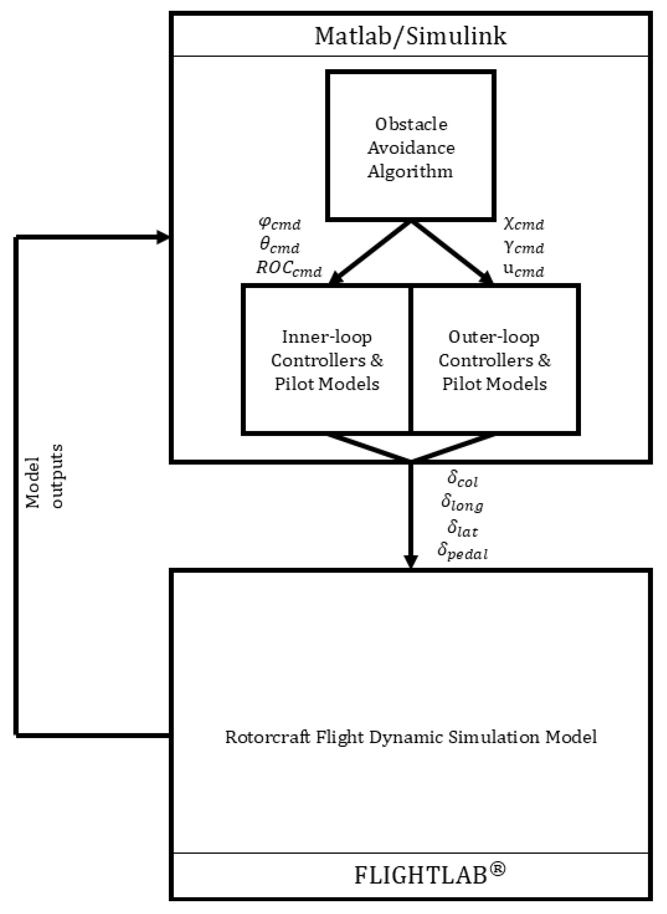
To test the performance of the methodologies in terms of obstacle avoidance and mission completion within the specified time interval capability, and to perform sensitivity analysis to determine key design parameters, several desktop simulations were conducted. For this purpose, both the LTI model extracted using the FLIGHTLAB^® generic helicopter model and the nonlinear model itself were used, and the simulations were performed in the MATLAB/Simulink environment. A block diagram of the desktop simulation setup is shown in Figure 5.

Different pilot models are used to complete the simulations. The pilot models based on the crossover model [37,38] are used to give commands. The transfer function of the pilot model is shown in Equation (26), where $K_p$ is the pilot gain, $T_L$ and $T_I$ are lead-lag time constants, and ${\tau }_e$ is the time delay. These parameters for each pilot are selected as listed in

Table 2. Pilot models.

Pilot	${\mathit{T}}_{\mathit{L}}$ [s]	${\mathit{T}}_{\mathit{I}}$ [s]	${\mathit{\tau }}_{\mathit{e}}$ [s]
Pilot A	0.2	0.2	0.2
Pilot B	0.1	0.3	0.3

. The pilot gains are the same for both pilot models.

$$Y_p\left(s\right)=K_p{\displaystyle \frac{1+T_{L}s}{1+T_{I}s}}.e^{-{\tau }_{e}s}$$

(26)

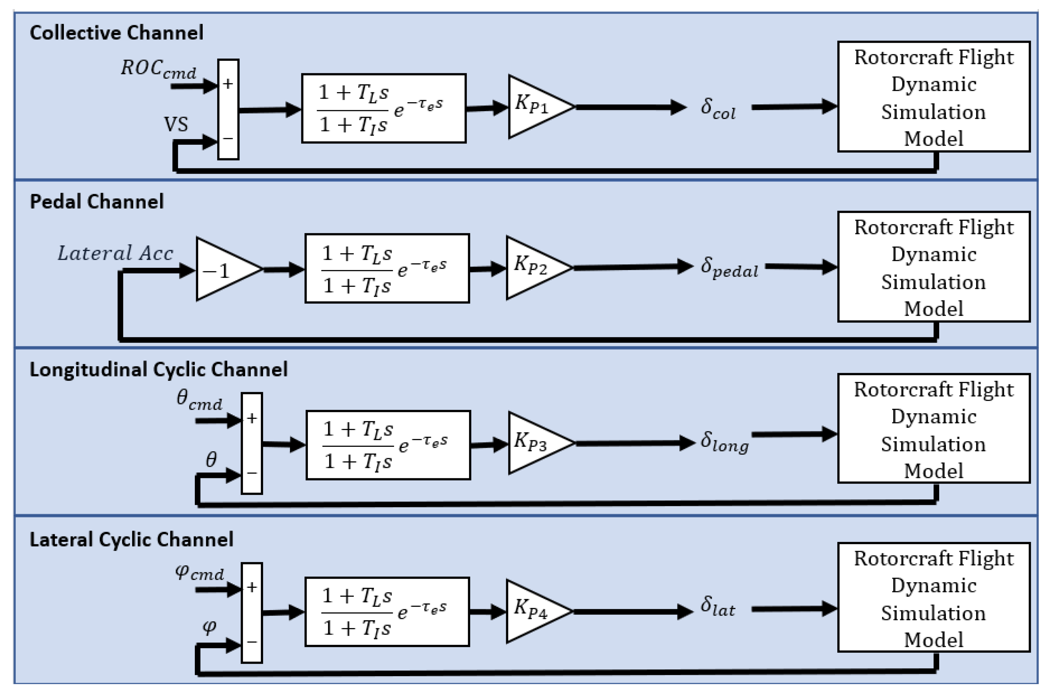
The architecture of the controllers consists of four input channels. The following control architecture is used for inner-loop guidance:

• The collective channel tracks the rate of climb guidance. The pilot model finds the appropriate collective input.
• In the pedal channel, zero lateral acceleration is achieved for a forward speed greater than 60 knots. The pilot model finds the required pedal input for zero lateral acceleration.
• In the longitudinal cyclic channel, the pitch angle guidance is followed. The pilot model finds the required longitudinal cyclic input for that pitch angle.
• In the lateral cyclic channel, the pilot model follows the bank angle guidance.

The inner-loop controller architecture is given in Figure 6.

The gains of the inner-loop pilot models used in this study are given in

Table 3. Inner-loop controller gains.

${\mathit{K}}_{\mathit{P}1}$	${\mathit{K}}_{\mathit{P}2}$	${\mathit{K}}_{\mathit{P}3}$	${\mathit{K}}_{\mathit{P}4}$
1.5	−10	30	50

. The gains are arbitrarily selected to achieve successful obstacle avoidance maneuvers with minimal control movements, while maintaining stability.

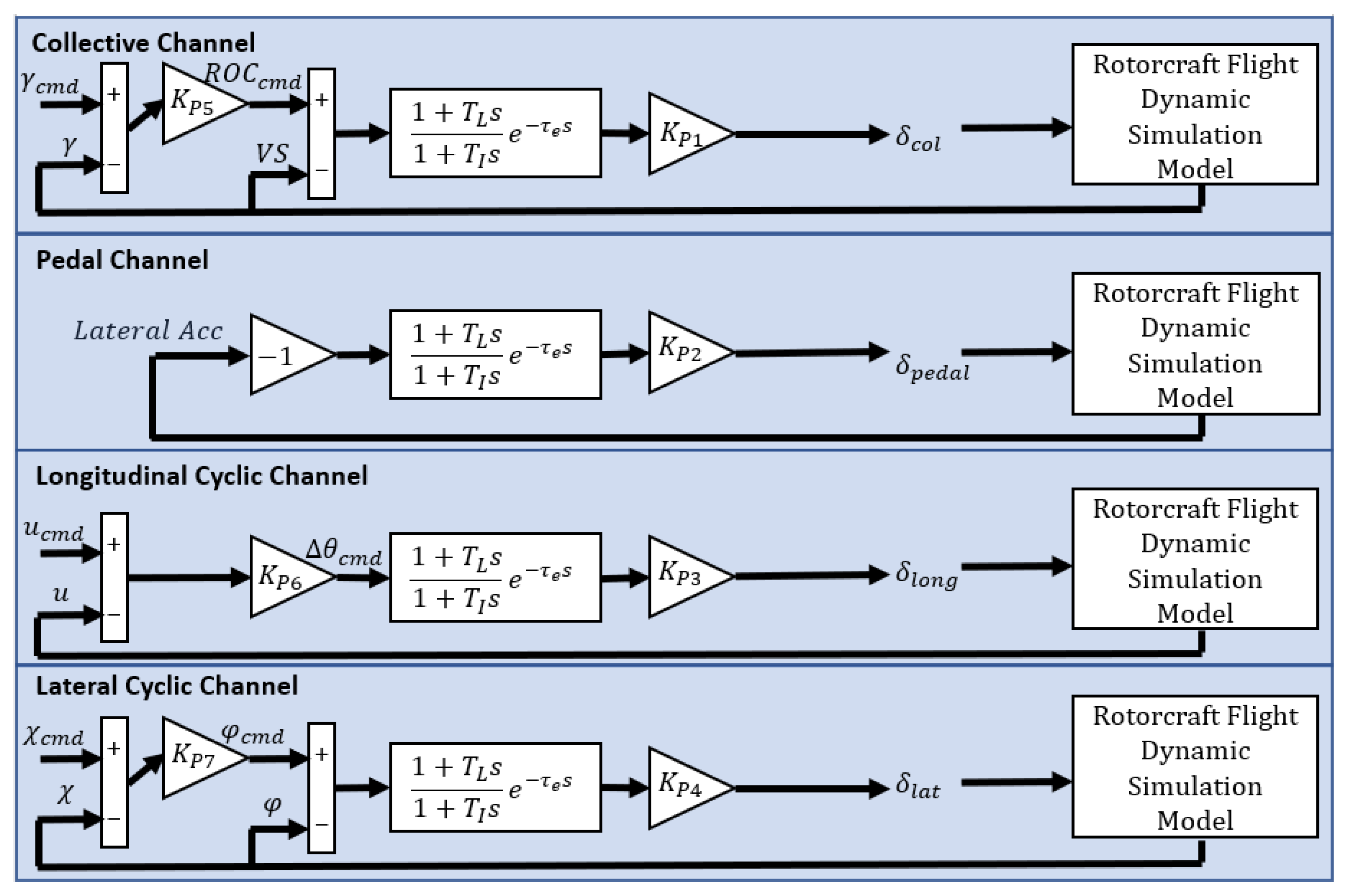
The following control architecture is used for the outer-loop guidance simulations:

• In the collective channel, the cascaded controller structure is used. The outer loop controls the flight path angle, and the inner loop controls the vertical speed.
• In the pedal channel, the pilot model achieves zero lateral acceleration.
• The longitudinal cyclic channel uses the cascaded controller structure. The deceleration trajectory guidance is followed in the outer loop. The inner loop controls the pitch angle.
• In the lateral cyclic channel, the cascaded controller structure is used. The outer loop controls the heading angle, and the inner loop controls the bank angle.

Lead-lag time constants and time delay are kept at zero except for the inner loops in the four input channels. The outer-loop controller architecture is given in Figure 7.

The gains of the outer-loop pilot models used in this study are given in

Table 4. Outer-loop controller gains.

${\mathit{K}}_{\mathit{P}1}$	${\mathit{K}}_{\mathit{P}2}$	${\mathit{K}}_{\mathit{P}3}$	${\mathit{K}}_{\mathit{P}4}$	${\mathit{K}}_{\mathit{P}5}$	${\mathit{K}}_{\mathit{P}6}$	${\mathit{K}}_{\mathit{P}7}$
1.5	−10	30	50	150	−0.01	2

. Similar to inner-loop pilot models, gains of the outer-loop pilot models are selected arbitrarily to achieve successful obstacle avoidance maneuvers with minimal control movements and without compromising stability.

4.2. Sensitivity Analysis and Design Parameter Selection

Safety Bubble’s Radius, Safety Margin Above the Obstacle, and Threshold Time, ${\tau }_m$

Since the sensitivity analysis required many consecutive simulations, they were performed using the LTI model extracted from the FLIGHTLAB^® generic helicopter model in 80 knots forward flight trim condition with zero sideslip and with different values of ${\tau }_m$. In the simulations, a sufficient initial distance between the obstacle and the helicopter is maintained, and the sizes and positions of the obstacles are varied with respect to the helicopter’s trajectory. The goal of this sensitivity analysis is to determine the two design parameters: the safety bubble’s radius ($R_S$) and the optimal threshold time (${\tau }_m$). The radius of the safety bubble is determined by repeating the simulations until the safety bubble is large enough that the helicopter does not hit the obstacle while performing the avoidance maneuver. The state vector is given by:

$$x^T=\left[uvwpqr\varphi \theta \psi \right]$$

(27)

where u, v, and w are the body-fixed velocities; p, q, and r are the angular rates, $\varphi$, $\theta$, and $\psi$ are the Euler angles. The control vector is:

$$u^T=\left[{\delta }_{long}{\delta }_{lat}{\delta }_{col}{\delta }_{pedal}\right]$$

(28)

where ${\delta }_{long}$ and ${\delta }_{lat}$ are the longitudinal and lateral cyclic inputs, ${\delta }_{col}$ is the collective input, and ${\delta }_{pedal}$ is the pedal input.

Sensitivity analyses are performed using obstacles with radii of 1 ft, 5 ft, 10 ft, 20 ft, 30 ft, 50 ft, 100 ft, 150 ft, 300 ft, 500 ft, 1000 ft, and 2000 ft. All obstacles are either centered on the helicopter’s trajectory or located slightly to the right of it. For each obstacle, the detection distance varies between 135 ft and 8100 ft, corresponding to time-to-collision values from 1 s to 60 s for a helicopter flying at 80 knots. The required radius for the safety bubble is determined for each case, with a fixed radius of 50 ft applied around the helicopter.

The analyses show that simulations performed with Pilot B consistently require a larger safety bubble. Therefore, these simulations are used to select a conservative safety bubble radius around the obstacle. Furthermore, the largest bank angle command occurs when the obstacle is centered with respect to the helicopter’s trajectory, which also requires a larger safety bubble. Consequently, the safety bubble radius is conservatively selected using the results of the centered obstacle simulations.

The key findings from these analyses are as follows:

1.

Obstacles with smaller radii (e.g., 50 ft) generate higher bank angle commands, making this method impractical for very small obstacles due to the helicopter’s structural and control limits. Therefore, bigger safety bubbles are needed for small obstacles.

2.

The generic helicopter model that is used in the simulations cannot make turns with a bank angle higher than approximately ${60}^{\circ }$ at 80 knots forward flight at constant altitude. Since the load factor is 2 when the bank angle is ${60}^{\circ }$, it is seen that the helicopter is limited to a maximum load factor of 2 for this flight condition.

3.

The ratio $\frac{R_S}{R_O}$ increases as the obstacle size decreases.

4.

As the distance from which the bank angle command is generated decreases, the bank angle command increases, further raising the $\frac{R_S}{R_O}$ ratio.

5.

Obstacles with radii greater than 1000 ft cannot be avoided if the command is generated with a threshold time ${\tau }_m<5$ s.

6.

For smoother turns, the command should ideally be given earlier. However, in highly congested environments, this may not always be feasible. Therefore, subsequent simulations use a threshold time of ${\tau }_m=10 s$ or higher, with an adaptive safety bubble radius that scales with the obstacle size given in

Table 5. Safety bubble radius.

Obstacle	${\mathit{R}}_{\mathit{S}}/{\mathit{R}}_{\mathit{O}}$	${\mathit{R}}_{\mathit{S}}/{\mathit{R}}_{\mathit{O}}$	${\mathit{R}}_{\mathit{S}}/{\mathit{R}}_{\mathit{O}}$	${\mathit{R}}_{\mathit{S}}/{\mathit{R}}_{\mathit{O}}$
Radius [ft]	${\mathit{\tau }}_{\mathit{m}}=\mathbf{10}$ s	${\mathit{\tau }}_{\mathit{m}}=\mathbf{20}$ s	${\mathit{\tau }}_{\mathit{m}}=\mathbf{30}$ s	${\mathit{\tau }}_{\mathit{m}}=\mathbf{60}$ s
1	68.8	48.7	41.1	31.8
5	15.2	11.2	9.7	7.9
10	8.5	6.4	5.7	4.8
20	5.1	4.0	3.6	3.2
30	3.9	3.2	2.9	2.6
50	3.0	2.5	2.3	2.1
100	2.2	1.9	1.8	1.6
150	1.9	1.6	1.6	1.5
300	1.5	1.4	1.3	1.3
500	1.4	1.3	1.2	1.2
1000	1.2	1.2	1.1	1.1
2000	1.2	1.1	1.1	1.1

. $\frac{R_S}{R_O}$ ratios for obstacles with 1 ft to 2000 ft radii are given in Table 5 when ${\tau }_m=10$ s, ${\tau }_m=20$ s, ${\tau }_m=30$ s, and ${\tau }_m=60$ s.

Similar to those performed for the bank angle guidance investigation, to determine the necessary safety margin above the obstacle for the rate of climb guidance, a series of sensitivity analyses is performed by changing the height of the obstacles, in addition to all the variables used in the aforementioned sensitivity analysis. However, it is observed that no significant pattern exists; therefore, as a safety margin, 30 ft above the height of the obstacles is used.

4.3. Results

In order to demonstrate and compare the performance of both inner-loop and outer-loop obstacle avoidance guidance methodologies in terms of obstacle avoidance and mission completion within the specified time interval capability, FLIGHTLAB^® high-fidelity nonlinear generic helicopter model is used. Desktop simulations begin with 80 knots forward flight trim conditions with zero sideslip. These simulations are performed using the “Pilot A” pilot models. In all simulations, the mission is plotted as the helicopter moves from the $(x_I,y_I)=(0,0)$ ft coordinates in the inertial frame at 150 ft altitude to the target point $(x_I,y_I)$ = (12,000 ± 50,0 ± 50) ft coordinates in the inertial frame at 150 ± 50 ft altitude. The number, size, and location of obstacles are kept as variables, generating different terrain scenarios. The number of obstacles changes between 5 to 20. The radius of each obstacle ranges from 50 to 500 ft, and the height from 50 to 1000 ft. The obstacles are randomly placed on the area with coordinates ranging from $(x_I,y_I)=(3000,-1500)$ ft to $(x_I,y_I)=(9000,1500)$ ft. In the simulations, the radius of the sphere surrounding the helicopter is set to 50 ft. Finally, ${\tau }_m$ is fixed to 30 s; in other words, the obstacle avoidance algorithm starts to work when the time-to-collision is less than 30 s. The selected limit value for ERITS is conservatively set at 420 ft/s, and the available maximum continuous power is 2796.7 hp.

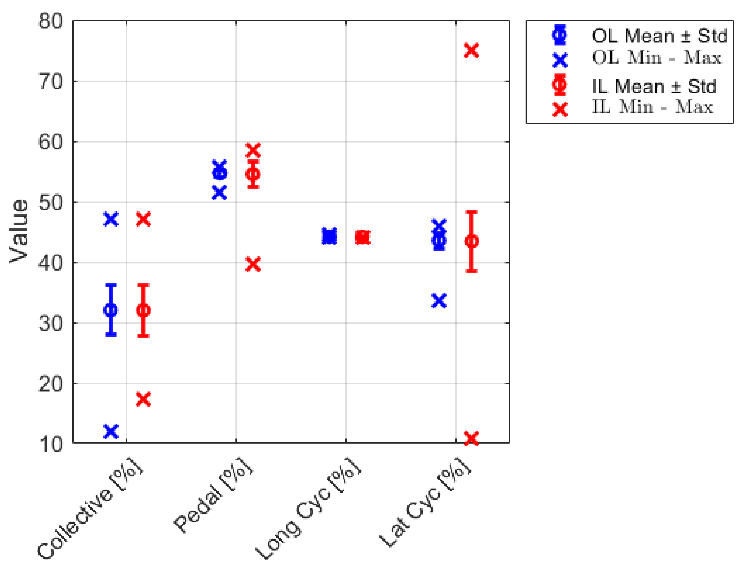
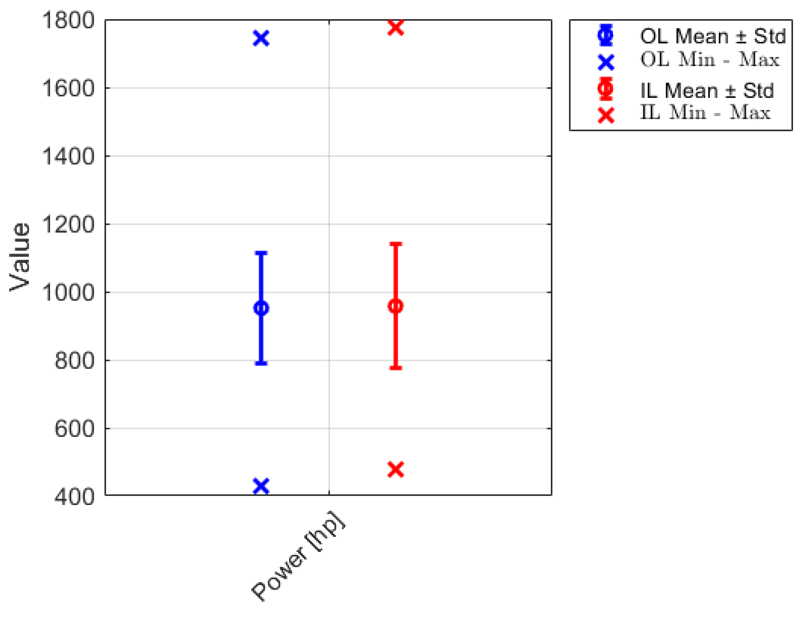
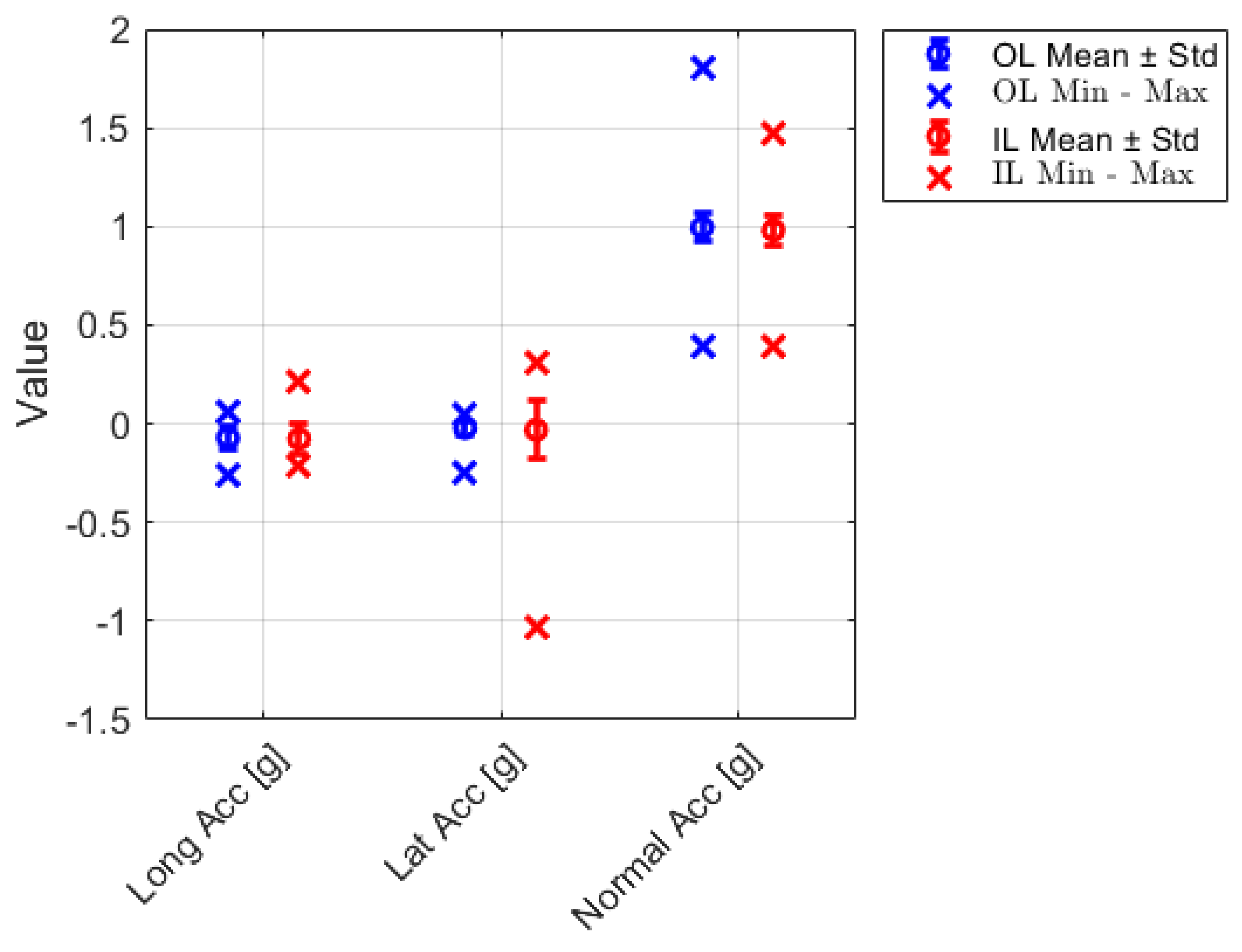
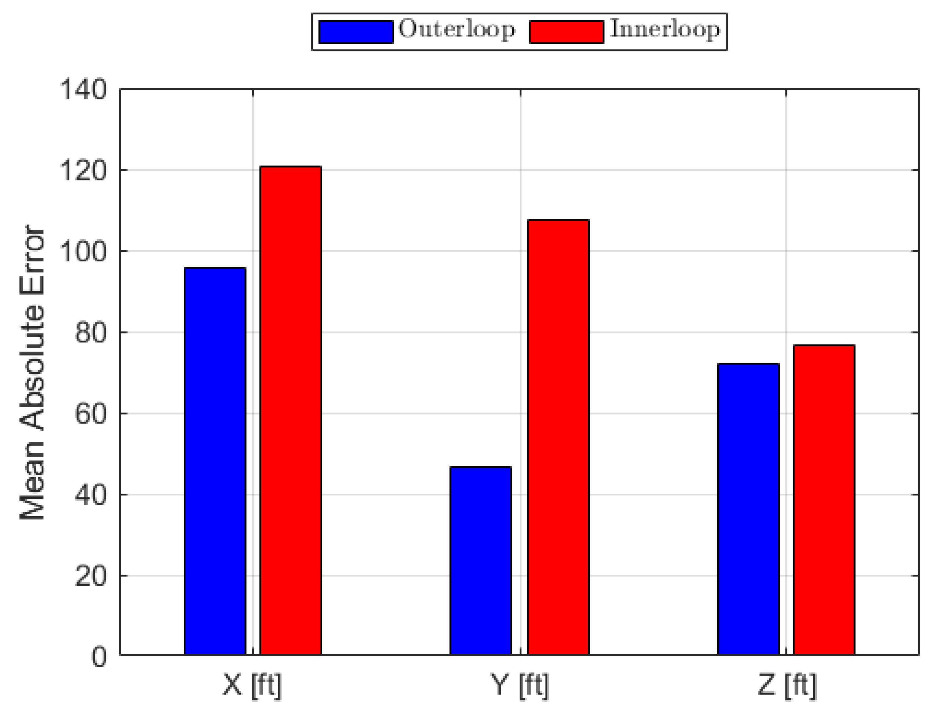
Figure 8, Figure 9, Figure 10 and Figure 11 compare the performance of the inner-loop and outer-loop guidance methodologies across control movements, power usage, accelerations, and deviation from the mission trajectory. Collectively, the results demonstrate that both methods can successfully complete obstacle avoidance missions while remaining within operational limits. However, distinct behavioral differences are observed between the two control architectures. Data distributions were obtained from successful simulations collected from 200 consecutive runs for both guidance methods. As the nonlinear model simulations used a rubber engine with no strict power limits, several of the simulations, though successful in completing the mission, were found to exceed the engine power limit of 2796.7 hp, perhaps due to the arbitrarily selected pilot model gains. As such, those simulation runs where power limit violations occurred were eliminated from the data distribution results shown in this paper, giving 44 simulations used in the inner-loop guidance evaluations and 37 simulations used in the outer-loop guidance evaluations. This suggests that inner-loop guidance was more successful in completing missions.

Figure 8 compares the control input distributions across the collective, pedal, longitudinal, and lateral cyclic channels. The outer-loop guidance exhibits smaller movements in the control inputs, whereas the inner-loop guidance requires larger lateral cyclic activity to follow the commanded guidance.

Figure 9 compares the required power distributions. The outer-loop guidance simulations display a slightly narrower mean range of standard devices, indicating slightly more stable power management and efficient energy usage.

Figure 10 presents the acceleration distributions along the longitudinal, lateral, and normal directions. The outer-loop guidance simulations maintain accelerations within moderate limits, resulting in smoother motion, while the inner-loop guidance simulations show higher peaks, particularly in the lateral axis, indicating more aggressive maneuvering. However, in one particular case, the outer-loop guidance simulation showed the highest normal acceleration peak, which is 1.8 g.

Figure 11 shows the mean absolute errors of the helicopter’s position in the longitudinal ($x_I$), lateral ($y_I$), and vertical ($z_I$) directions with respect to the initial mission trajectory, indicating the trajectory deviations. The outer-loop guidance yields smaller deviations from the mission trajectory across all axes. In contrast, inner-loop guidance exhibits higher mean absolute errors, especially along the lateral axis. This suggests that the outer-loop guidance achieves smoother path tracking, whereas the inner-loop guidance commands attitude angles directly, resulting in more abrupt corrections and increased positional deviation.

An overall mission-level comparison of the two methods reveals a difference: the outer-loop guidance completes the mission in 93 s, while the inner-loop guidance takes approximately 96 s. Without disruptions, a vehicle traveling at 80 knots would complete the mission in 88.9 s. Due to avoidance maneuvers, missions finish 4 to 7 s later than the theoretical time. A 3-s reduction in mean simulation time further demonstrates the outer-loop methodology’s efficiency in maintaining forward progress with smoother, energy-conscious maneuvers.

In terms of computation time, it is found that both methodologies have very little simulation time and can be used in real time when compared.

To further assess the robustness of each guidance methodology, the closest and farthest clearance distances from obstacles are collected in both the horizontal and vertical planes for both the inner-loop and outer-loop guidance simulations, based on 200 simulations each. For the inner-loop guidance, the closest clearance distance was 78.7 ft, and the farthest clearance distance was 3360.4 ft in the horizontal plane. The closest clearance distance was 11.3 ft, and the farthest clearance distance was 72.9 ft in the vertical plane. For the outer-loop guidance methodology, the closest and farthest clearance distances were 97.9 ft and 3911.7 ft, respectively, in the horizontal plane, and 15.8 ft and 30 ft, respectively, in the vertical plane. These results suggest that the outer-loop guidance maintains a larger minimum clearance and a wider horizontal safety corridor, while the inner-loop guidance provides greater vertical maneuvering freedom.

Table 6. Quantitative comparison of inner-loop and outer-loop obstacle avoidance guidance methodologies.

Metric	Inner-Loop Guidance	Outer-Loop Guidance
Number of successful runs	44/200	37/200
Mission completion time [s]	96	93
Control Activity Mean ± Std (Min-Max)
Collective [%]	$32\pm 4$  (17–47)	$32\pm 4$  (12–47)
Pedal [%]	$55\pm 2$  (40–59)	$55\pm 0.5$  (51.5–56)
Longitudinal Cyclic [%]	$44\pm 0.5$  (43-45)	$44\pm 0.5$  (43–45)
Lateral Cyclic [%]	$43\pm 5$  (11–75)	$43\pm 1$  (33–46)
Overall control behavior	Larger lateral activity	Smaller, smoother inputs
Trajectory deviation (MAE) in $x_I$ [ft]	121.0	96.0
Trajectory deviation (MAE) in $y_I$ [ft]	107.5	46.5
Trajectory deviation (MAE) in $z_I$ [ft]	77.0	72.0
Power Mean ± Std (Min-Max) [hp]	958 ± 181   (477–1778)	951 ± 161   (427–1743)
Longitudinal acceleration [g]	−0.08 ± 0.07	−0.07 ± 0.06
Lateral acceleration [g]	−0.03 ± 0.15	−0.02 ± 0.04
Normal acceleration [g]	1.0 ± 0.08	1.0 ± 0.07
Closest horizontal clearance [ft]	78.7	97.9
Farthest horizontal clearance [ft]	3360.4	3911.7
Closest vertical clearance [ft]	11.3	15.8
Farthest vertical clearance [ft]	72.9	30.0

provides a summary of the key performance metrics investigated for both methodologies.

4.3.1. Inner-Loop Guidance Example Desktop Simulation Results

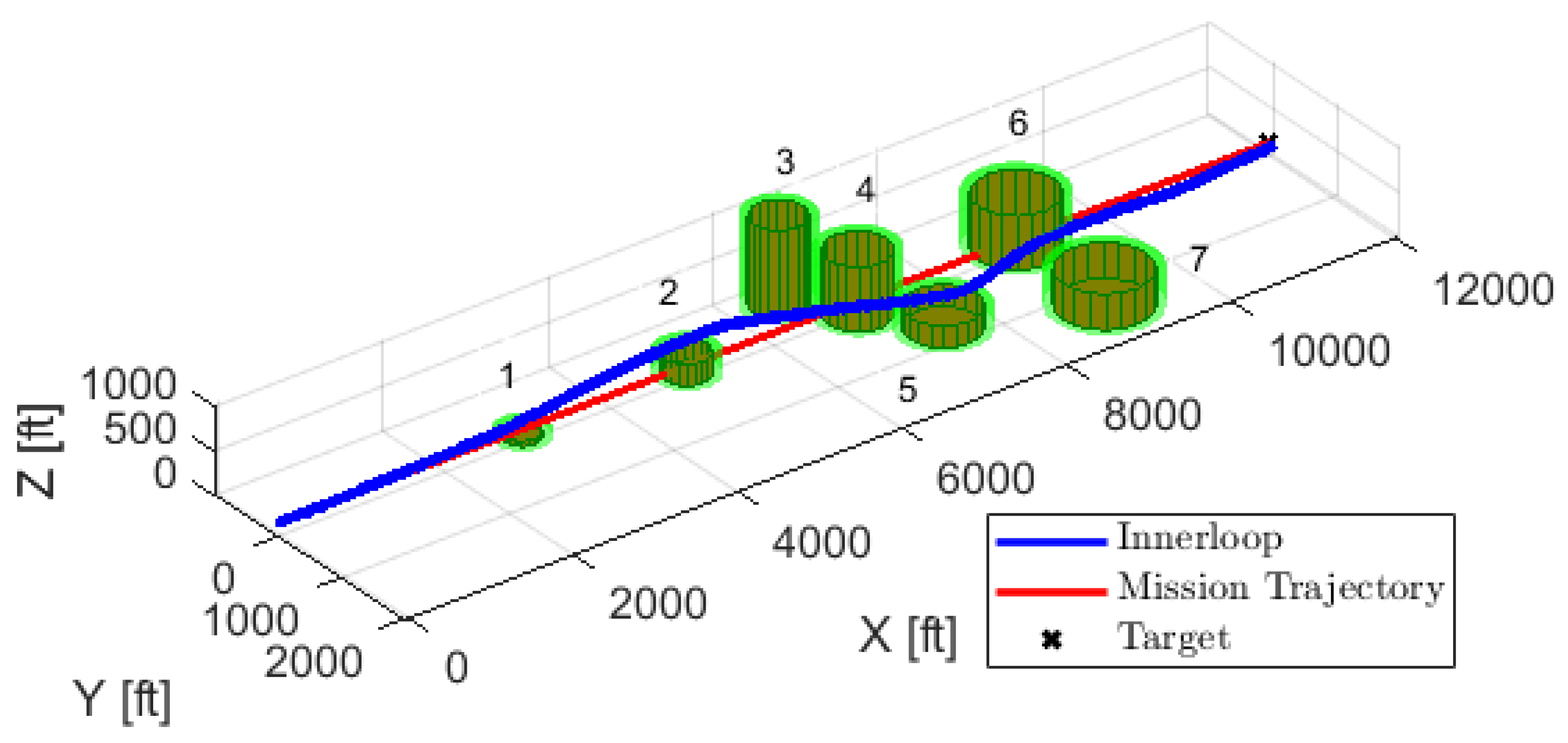
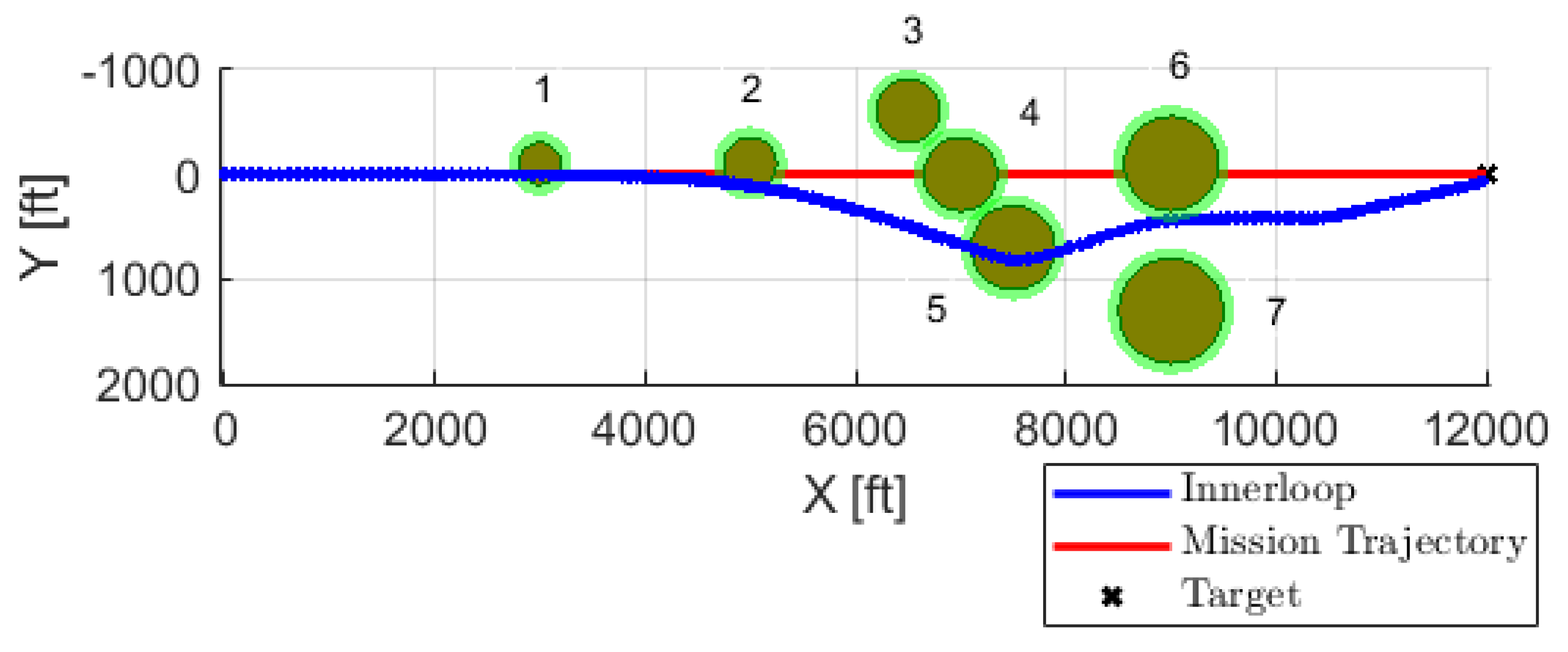
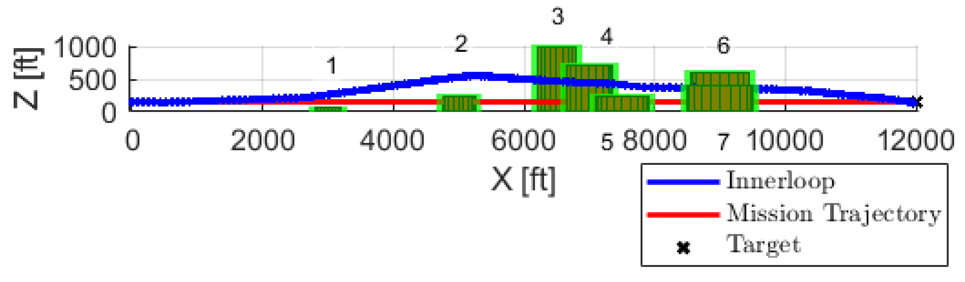
The results of a sample simulation performed for the inner-loop guidance from the top, side, and isometric views are shown in Figure 12, Figure 13, and Figure 14, respectively. For this simulation, the obstacle specifications are given in

Table 7. Environment data.

Obstacle Number	Radius [ft]	Height [ft]	Location (${\mathit{x}}_{\mathit{I}}$,${\mathit{y}}_{\mathit{I}}$) [ft]
1	200	60	(3000, −100)
2	250	240	(5000, −100)
3	300	1000	(6500, −600)
4	350	720	(7000, 0)
5	400	240	(7500, 700)
6	450	600	(9000, −100)
7	500	400	(9000, 1300)

. The obstacle numbers can be seen in Figure 12, Figure 13 and Figure 14.

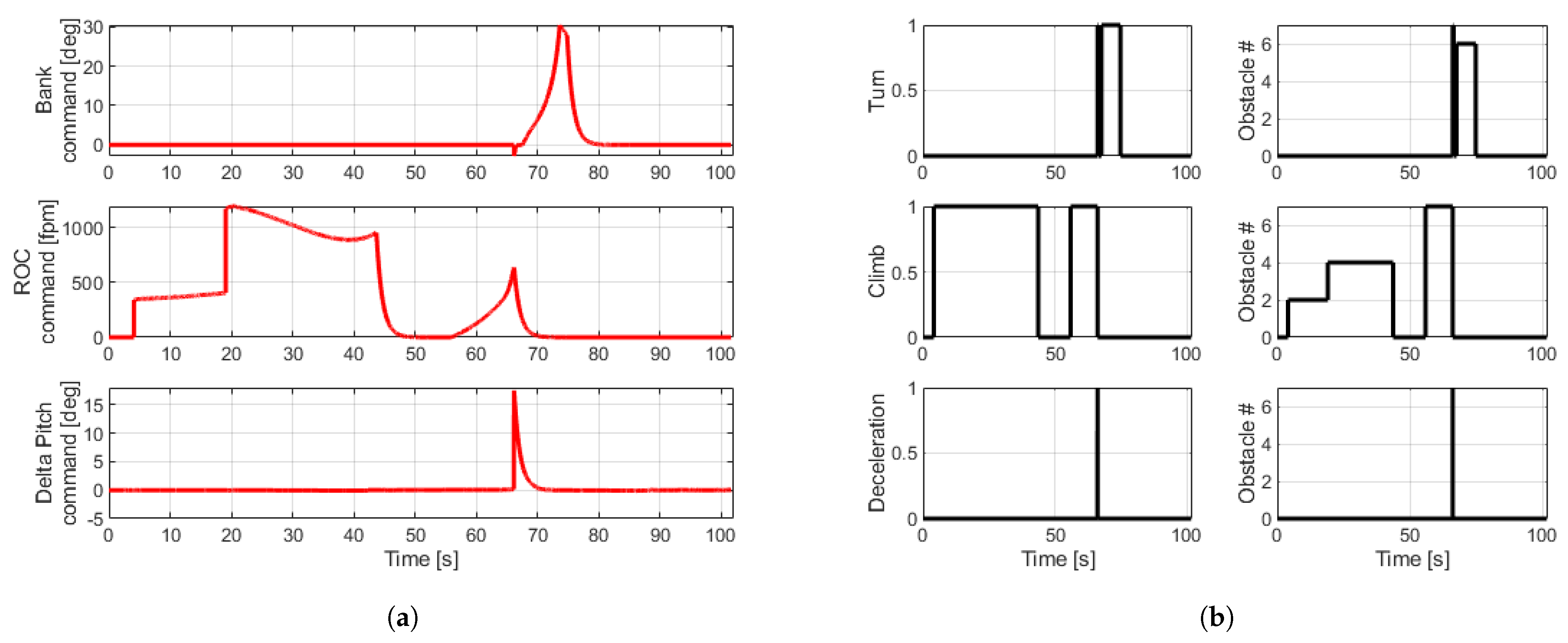
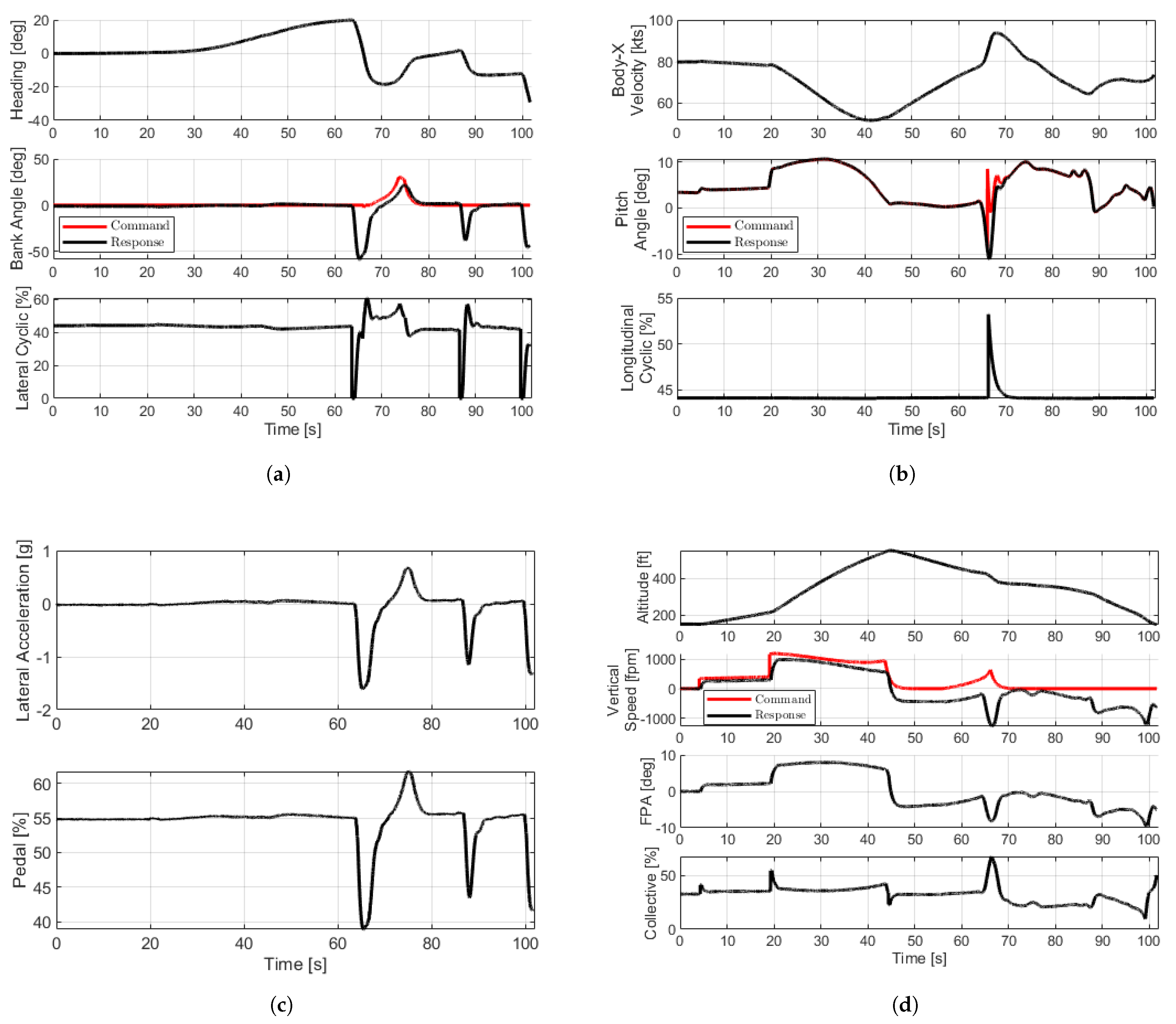
As can be seen, the trajectory resulting from the inner-loop guidance methods differs from the mission trajectory. Figure 15 shows the obstacle avoidance maneuvers, as well as the turn, climb, and deceleration commands that lead the helicopter to this different trajectory. It also illustrates the obstacles that are avoided by performing these maneuvers. Figure 16 shows the helicopter response in all four channels for inner-loop guidance simulations. Pilot models follow the bank angle, the rate of climb, and the pitch angle guidance for the inner-loop guidance.

In this example, the helicopter performs three obstacle avoidance maneuvers: turning, climbing, and decelerating while en route to the target. Since Obstacle #1 lies below the helicopter’s initial altitude, it is passed over without any maneuver. Then, the climb maneuver is initiated upon detecting Obstacle #2. Since the helicopter has enough power, it climbs over Obstacle #2 at its current speed. Then, Obstacle #4 is detected at 19 s, as it is on the helicopter’s trajectory. To avoid Obstacle #4, the climb maneuver continues with an increased rate of climb. Because the excess power is enough to climb over Obstacle #4, the avoidance maneuver is started at 80 knots. An increased yaw rate occurs with increased torque, causing the helicopter to move to the right during the climb maneuver. The heading changes and the avoidance maneuver stops before reaching Obstacle #4. As the Obstacle #5 is below the helicopter, it moves over it without any maneuvers. At 53 s, it encounters Obstacle #7 and initiates a climbing avoidance maneuver to avoid it. At 65 s, the helicopter turns toward the target while still climbing. However, this maneuver causes the helicopter to lose altitude. Therefore, it first slows down in order to continue the climbing maneuver at lower power settings. However, because it cannot climb over Obstacle #7, it then turns slightly left to avoid it. These three maneuvers occur in less than a second. As it avoids Obstacle #7, it moves through the gap between Obstacle #6 and Obstacle #7. When the helicopter faces Obstacle #6, it cannot climb over it, so a turning avoidance maneuver is initiated. After leaving all the obstacles behind, at 75 s, the helicopter begins to lose altitude and make maneuvers to complete the mission, and finally reaches the target at almost 102 s.

4.3.2. Outer-Loop Guidance Example Desktop Simulation Results

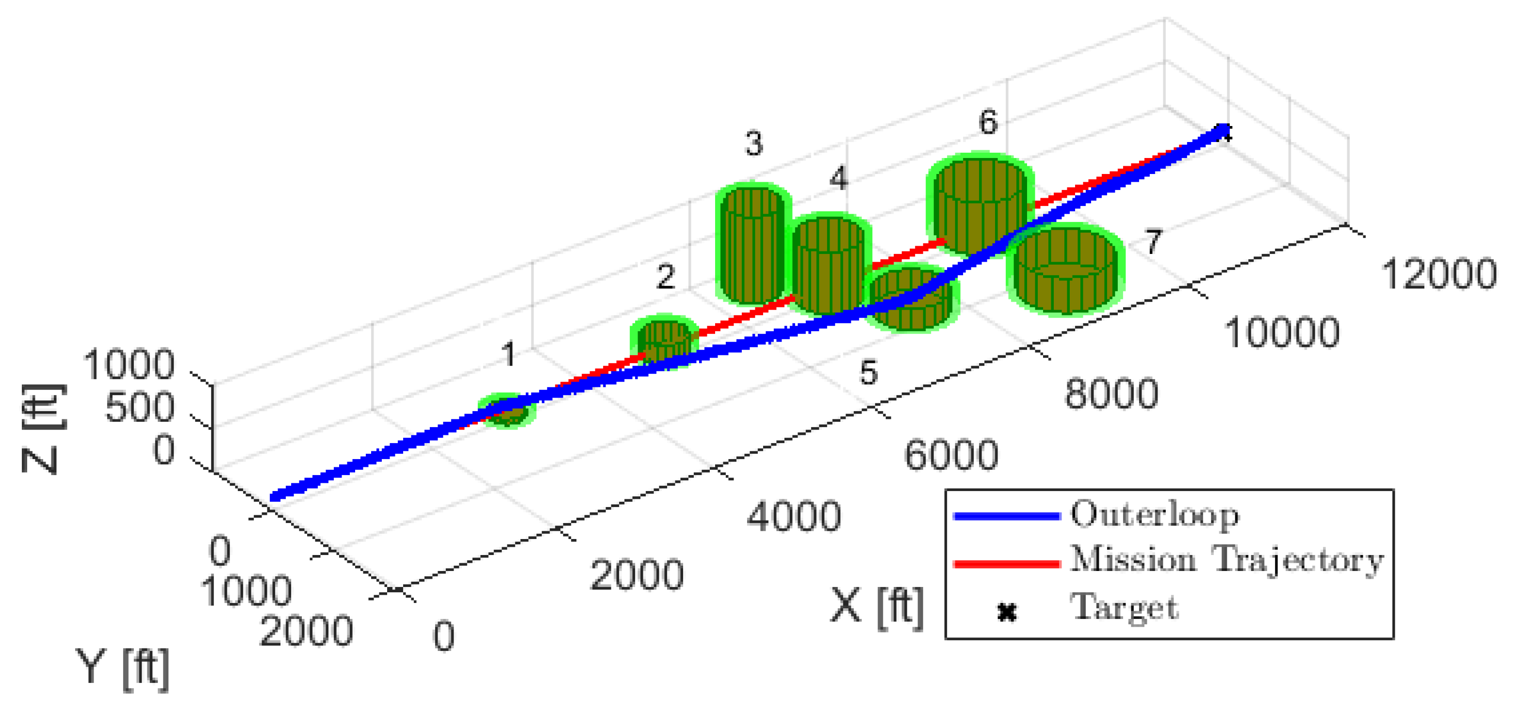
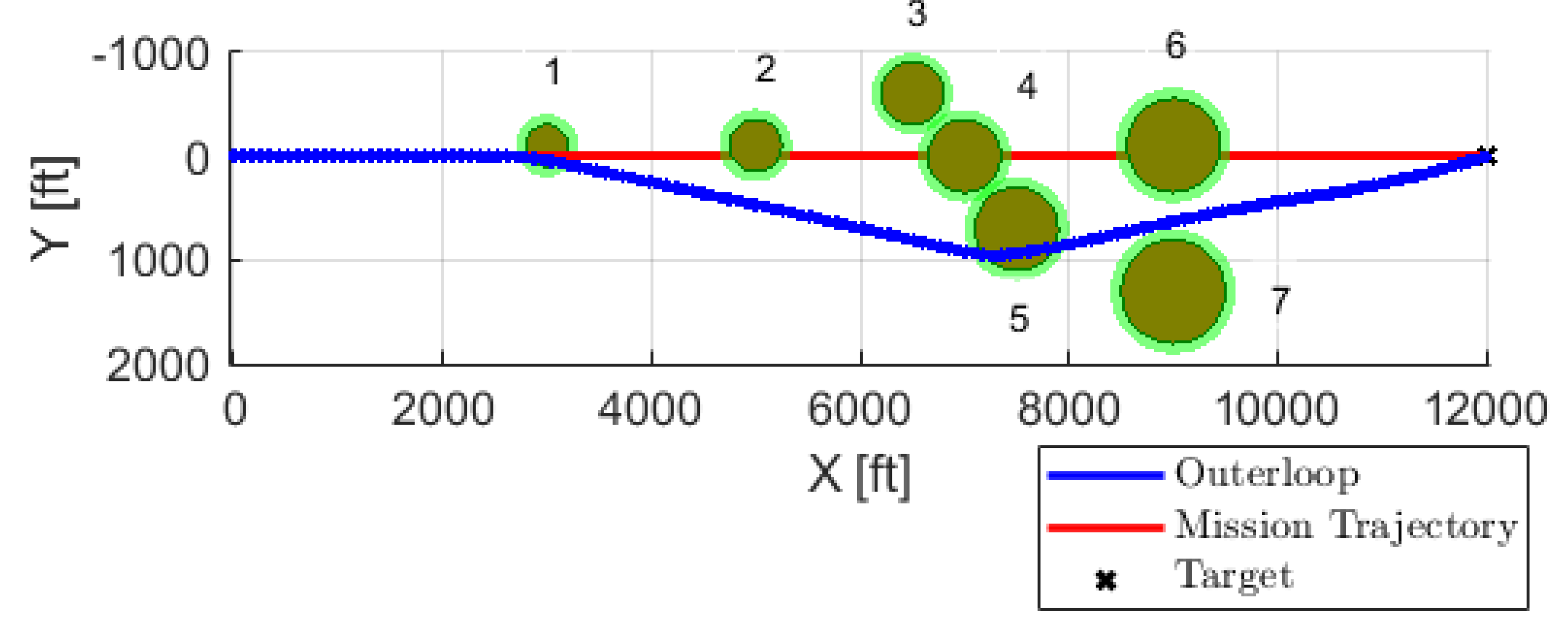
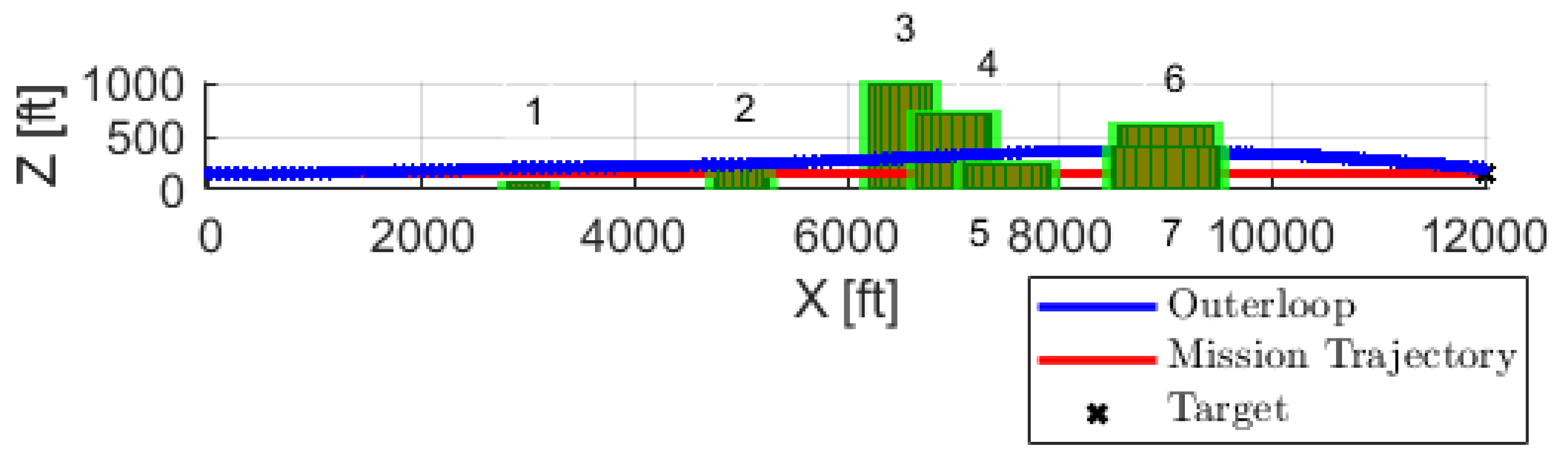
The results of the simulation performed for the outer-loop guidance from the top, side, and isometric views are shown in Figure 17, Figure 18 and Figure 19, respectively. In this simulation, the same terrain data given in Table 7 is used.

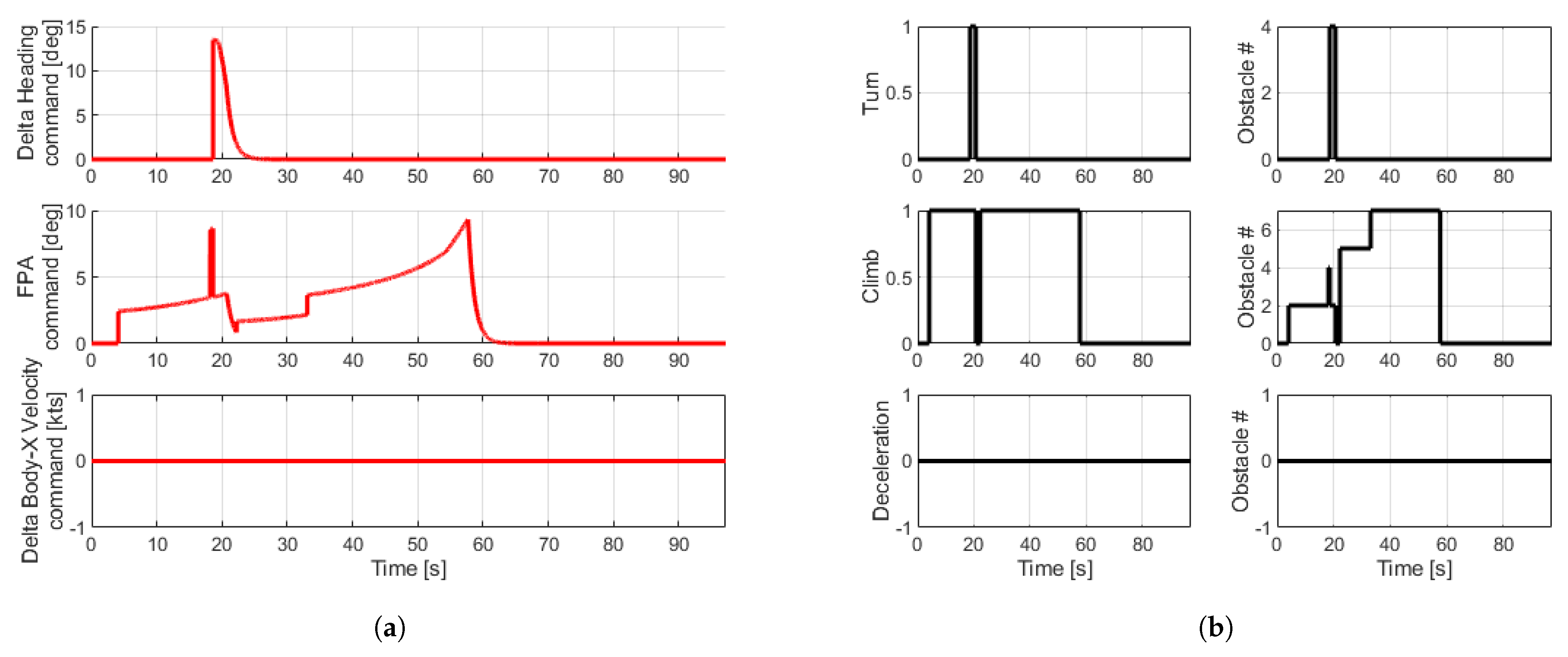
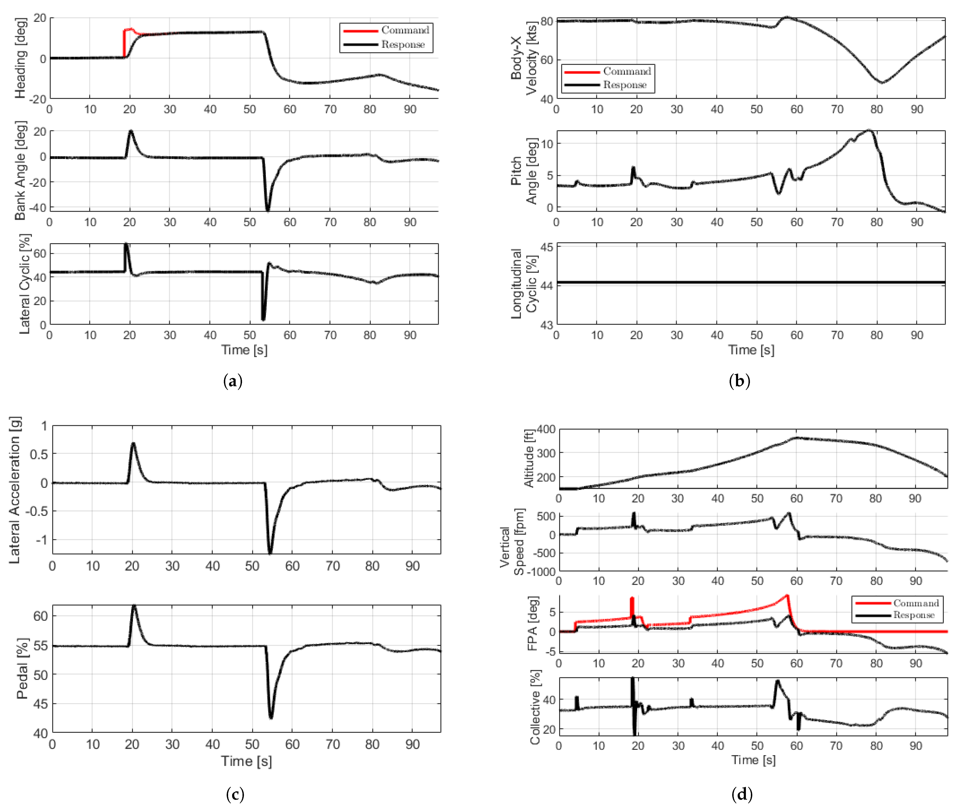
Figure 20 shows the obstacle avoidance maneuvers, as well as the turn, climb, and deceleration commands for outer-loop guidance simulations. It also illustrates the obstacles that are avoided by performing these maneuvers. Figure 21 shows the helicopter response in all four channels.

In the outer-loop guidance simulation example, the helicopter performs two obstacle avoidance maneuvers while navigating to the target: turning and climbing. Avoidance maneuvers are very similar to the inner-loop avoidance maneuver for Obstacles #1 and #2. Since excess power is insufficient even if the helicopter is decelerated, a turn maneuver is performed to avoid Obstacle #4. Due to Obstacle #3, a larger bank angle is required to avoid Obstacles #3 and #4 if a left turn is performed. Therefore, bank angle guidance is generated to avoid Obstacle #4 by making a right turn. After avoiding Obstacle #4, the helicopter starts to climb over, first Obstacle #5, then Obstacle #7, which are both in front of the helicopter. Once the helicopter reaches an altitude higher than Obstacle #7, it turns toward the target and begins to move through the gap between Obstacle #6 and #7. After leaving all obstacles behind in 57 s, the helicopter begins to lose altitude in order to complete the mission. Finally, it reaches the target at around 97 s.

4.4. Conclusions

This study shows an obstacle avoidance methodology based on the Tau theory. The results of the desktop simulations lead to the following key conclusions.

1.

An inner-loop and an outer-loop guidance methodologies were developed for helicopter obstacle avoidance that integrate turning, climbing, and deceleration maneuvers, guided by a decision logic framework. This framework evaluates maneuver feasibility based on available excess power and aerodynamic limits.

2.

A decision-making algorithm was implemented to evaluate all obstacles on the trajectory, determine the most suitable avoidance strategy, and execute smooth transitions between maneuvers while maintaining the aircraft within operational limits.

3.

Desktop simulations using FLIGHTLAB-based nonlinear helicopter models and pilot transfer function models confirmed the feasibility of both of the guidance methodologies for dynamic, low-altitude, high-speed terrain-following flights, especially in obstacle-dense, degraded visual environments. Both inner-loop and outer-loop guidance approaches successfully complete the mission in the simulated environment across varied terrain scenarios.

4.

The outer-loop guidance demonstrates superior smoothness, trajectory precision, and energy efficiency, while the inner-loop guidance offers faster attitude-level response and higher success rates in dense obstacle environments.

5.

These results collectively validate the readiness of the Tau-theory-based guidance framework for integration into real-world applications. Extending the framework for fully autonomous obstacle avoidance or optionally-piloted vehicle applications represents a promising avenue for broader operational deployment.

Despite its demonstrated feasibility and efficiency, several aspects need further investigation. The current framework assumes idealized sensor data and instantaneous obstacle detection; therefore, future studies should include sensor latency, field-of-view limitations, and environmental noise to assess robustness. Additionally, pilot-in-the-loop evaluations are necessary to analyze the influence of pilot cueing applications on pilot workload under a DVE. Finally, incorporating tuned and more sophisticated control algorithms can improve maneuver optimization and successful mission completion. Addressing these challenges will further advance the readiness of the proposed guidance framework for operational use in both manned and autonomous rotorcraft applications.