A Nonlinear Model of Three-Layer Groundwater Flow with Evaporation Dependent on the Critical Groundwater Level

Abstract

A nonlinear mathematical model is developed for unsteady groundwater flow in a three-layer heterogeneous aquifer system, comprising a confined aquifer, a covering layer, and a weakly permeable barrier. The model incorporates infiltration and evaporation governed by the M.M. Krylov–S.F. Averyanov law, where evaporation intensity depends on a critical groundwater level. Governing equations are nondimensionalized and solved using the alternating direction implicit (ADI) method with quasi-linearization to treat nonlinearities. Periodic variations in precipitation and evaporation are considered, alongside variable boundary permeabilities. The approach enables realistic simulation of multi-layer aquifer dynamics under diverse climatic and hydrogeological conditions, offering a robust tool for sustainable groundwater management, drought risk assessment, and aquifer protection strategies.

1. Introduction

Groundwater resources constitute the primary source of freshwater for over 2.5 billion people globally and support approximately 40% of irrigated agriculture worldwide [1,2]. In arid and semi-arid regions, where surface water resources are limited or seasonally variable, groundwater becomes the sole reliable water source for domestic, agricultural, and industrial purposes [3,4,5]. The sustainable management of these resources requires accurate mathematical models capable of simulating complex groundwater flow dynamics under various hydrogeological conditions.

Multi-layered aquifer systems represent a prevalent hydrogeological configuration in sedimentary basins worldwide. These systems typically consist of alternating sequences of high-permeability aquifers and low-permeability aquitards, creating complex three-dimensional flow patterns that challenge conventional modeling approaches [6,7]. The accurate simulation of such systems becomes particularly critical in regions experiencing rapid groundwater depletion, where understanding vertical flow exchanges between layers determines the long-term sustainability of water extraction strategies. The interaction between groundwater and atmospheric processes through evaporation and infiltration fundamentally controls the water balance in shallow aquifer systems [8]. In areas where groundwater levels are shallow, evaporation can account for 50–70% of the total groundwater discharge. Therefore, an accurate representation of evaporation is of crucial importance for a reliable assessment of water resources [9,10,11,12,13,14].

2. Literature Review, Research Gaps, and Contributions

2.1. Literature Review

The mathematical modeling of multi-layered groundwater systems has undergone substantial evolution over the past five decades, progressing from simplified analytical solutions to sophisticated numerical frameworks capable of simulating complex heterogeneous formations. Early foundational work by Bear [7] and Hantush [8] established analytical solutions for steady-state flow in multi-layer systems under restrictive assumptions of homogeneity and simplified boundary conditions. While these classical approaches provided valuable insights into fundamental flow patterns, their applicability remained limited to idealized configurations that rarely reflect natural hydrogeological complexity.

The development of numerical methods marked a paradigm shift in multi-layer aquifer modeling capabilities. Wang and Anderson pioneered the application of finite difference methods to multi-layer systems, establishing the theoretical foundation for what would become MODFLOW, now the international standard for groundwater modeling [15]. Recent advances documented by Langevin et al. [16] in MODFLOW 6 introduce generalized control-volume finite-difference approaches that support unstructured grids and enable simulation of complex geological geometries previously impossible with structured grid approaches. The capability to handle over 8.1 billion unknowns demonstrates the dramatic expansion in computational capacity that now enables continental-scale multi-layer simulations [17].

Significant contributions to multi-layer aquifer modeling have emerged from analytical and semi-analytical approaches. Ravshanov et al. [18] developed approximate analytical solutions for fluid filtration problems in multilayer porous media, providing valuable benchmarks for numerical model validation. Their subsequent work on unsteady filtration in three-layer bounded reservoirs introduced analytical solutions that capture transient behavior while maintaining computational efficiency. These analytical frameworks have proven particularly useful for preliminary assessments and verification of more complex numerical models.

The numerical modeling of groundwater flow in heterogeneous multi-layer systems has advanced through various computational approaches. Ravshanov and colleagues demonstrated the effectiveness of numerical algorithms for studying fluid filtration in three-layer interacting pressure porous formations, revealing complex inter-layer exchange mechanisms [19]. Their work on numerical and mathematical modeling of changes in groundwater levels in two-layer media provided insights into the coupled nature of confined and unconfined aquifer interactions. These studies have highlighted the importance of accurately representing vertical hydraulic connections between layers, particularly in systems with significant pressure differentials.

The coupling of surface and subsurface processes represents a critical advancement in hydrological system modeling. Recent global-scale two-layer transient groundwater models have successfully simulated lateral groundwater flows while incorporating vertical aquifer structure information, identifying hotspot regions of groundwater depletion worldwide [20,21]. The integration of big geological data has enabled more detailed stratigraphic modeling, with studies incorporating over 29,000 well logs to construct multi-layer representations of complex aquifer systems [22].

Understanding vertical flow exchange mechanisms between aquifer layers has received renewed attention in recent literature. Studies of compaction in multi-layer aquifer systems due to groundwater withdrawal have revealed that subsidence can be contributed by compaction in different layers, with single-layer groundwater users responsible for large-area compaction while significant local compaction can be attributed to multi-layer users [23]. The analytical quasi-three-dimensional groundwater models coupled with deformation models have proven effective in clarifying the causes and estimating the amount of compaction in systems with spatially and temporally varying pumping activities [24].

The representation of complex boundary conditions and nonlinear processes in groundwater models has evolved significantly. Ravshanov and Daliev [18,19] developed nonlinear mathematical models to predict changes in underground water level and salt concentration, incorporating the coupled effects of evaporation and salt transport. Their work demonstrated that nonlinear formulations are essential for accurately representing systems where evaporation and salt accumulation create feedback mechanisms that influence groundwater dynamics. Advanced numerical techniques for solving nonlinear groundwater flow equations have been developed to address computational challenges. These techniques have proven particularly valuable for problems involving multiple interacting nonlinear processes.

The representation of evapotranspiration processes in groundwater models remains an area of active development. Despite the fundamental importance of evaporation in controlling shallow groundwater dynamics, most contemporary models employ simplified formulations that fail to capture the full nonlinearity of the evaporation-depth relationship [25,26]. The classical Krylov–Averyanov law [14], while physically based, is rarely implemented in its complete nonlinear form due to numerical challenges in solving the resulting equations. This simplification can lead to errors exceeding 30% in water balance calculations for systems with shallow water tables [27].

Recent advances in machine learning approaches have shown promise for groundwater level prediction. Deep learning models, including Long Short-Term Memory networks and automated machine learning frameworks, have achieved high accuracy in forecasting water table fluctuations [28]. Studies have demonstrated that these AI-driven models can effectively handle sparse, brief data to mimic irregular and non-linear time series with classification accuracies exceeding 0.93 [29]. However, these data-driven approaches often lack the physical basis necessary for understanding complex process interactions and cannot adequately represent the nonlinear coupling between evaporation, infiltration, and vertical drainage that characterizes multi-layer systems [30,31].

2.2. Research Gaps

Despite substantial advances in multi-layer groundwater modeling, critical gaps remain that limit the accurate simulation of complex hydrogeological systems under realistic conditions. These gaps span theoretical formulations, numerical implementations, and practical applications, collectively constraining our ability to develop reliable predictions for water resource management.

The treatment of evaporation processes in multi-layer models remains fundamentally incomplete. While the Krylov–Averyanov law provides a physically based framework for relating evaporation rate to groundwater depth, its full nonlinear implementation is absent from major modeling platforms including MODFLOW and ParFlow [16,17]. Current models typically employ either constant evaporation rates or simplified linear decay functions that fail to capture the critical depth threshold behavior that governs actual evaporation processes [32]. This simplification can lead to substantial errors in water balance calculations for systems with shallow water tables, yet the numerical challenges of implementing the complete nonlinear formulation have prevented its widespread adoption.

The simultaneous consideration of vertical drainage, infiltration, and nonlinear evaporation within a unified mathematical framework represents a significant unaddressed challenge. Existing models typically treat these processes independently or through loosely coupled approaches that may violate mass conservation principles [33]. The strong nonlinear coupling between these processes, particularly under transient conditions with varying precipitation and evaporation patterns, requires solution techniques that maintain numerical stability while preserving physical consistency [34].

Boundary conditions in multi-layer models generally assume constant or simple time-varying permeabilities that inadequately represent the complex dynamics at geological interfaces. River–aquifer boundaries, in particular, exhibit spatial and temporal variations in hydraulic conductivity due to sediment deposition, erosion, and biological processes that can alter effective permeability by orders of magnitude [35,36]. Current modeling approaches lack mechanisms for incorporating these variable boundary permeabilities in a physically consistent manner.

The dimensionalization of governing equations for multi-layer systems has received insufficient attention despite its importance for model generalization and numerical efficiency. Most existing models operate in dimensional form, requiring case-specific parameter adjustments that complicate model transferability and comparison across different hydrogeological settings [37]. The development of properly scaled dimensionless formulations would enable more systematic analysis of controlling parameters and facilitate the identification of similarity solutions applicable across diverse aquifer systems [38].

2.3. Contributions

This research advances the field of multi-layer groundwater modeling through four primary contributions that address fundamental gaps in current modeling capabilities while maintaining computational tractability for practical applications.

First, this study develops a comprehensive nonlinear mathematical model that fully implements the M.M. Krylov–S.F. Averyanov evaporation law with its critical depth dependency within a three-layer heterogeneous aquifer system framework. Unlike existing simplified approaches [14], our formulation preserves the complete nonlinear relationship between evaporation intensity and groundwater depth, including the threshold behavior at critical depth where evaporation ceases. This achievement enables reliable modeling of water balance in areas with shallow water levels, where evaporation serves as the primary mechanism of water loss.

Second, this research introduces a systematic dimensionless formulation of the governing equations that enables universal application across different spatial scales and hydrogeological settings. Through careful selection of characteristic scales based on system properties, we transform the dimensional equations into a canonical form that reveals the fundamental dimensionless parameters controlling system behavior. This transformation facilitates numerical solution while providing insight into the relative importance of various physical processes.

Third, this research implements an advanced numerical solution strategy combining the alternating direction implicit method with quasi-linearization techniques specifically adapted for handling the strong nonlinearities arising from the Krylov–Averyanov law. The quasi-linearization approach iteratively updates the nonlinear coefficients while maintaining the favorable stability properties of the ADI scheme, achieving convergence rates superior to traditional iterative methods [39].

Fourth, the model is extended to incorporate temporally and spatially variable boundary permeabilities that represent realistic conditions at river–aquifer interfaces and geological contacts. The formulation allows hydraulic conductivity at boundaries to vary as functions of both space and time, capturing effects such as seasonal sediment deposition and clogging-unclogging cycles. This capability enables simulation of complex boundary processes that significantly influence groundwater flow patterns but have been inadequately represented in previous multi-layer models [40].

3. Methodology

3.1. Problem Formulation

The mathematical formulation of groundwater flow in multi-layered aquifer systems requires careful consideration of the physical processes occurring within each hydrogeological unit and the interactions between adjacent layers. This section presents a comprehensive mathematical model for unsteady groundwater flow in a three-layer heterogeneous system that incorporates the complex nonlinear processes governing water movement in natural aquifer systems.

3.1.1. Physical System Description

We consider a three-dimensional heterogeneous aquifer system consisting of three distinct hydrogeological units with contrasting hydraulic properties. The system comprises a main confined aquifer of thickness $m$, overlain by a semi-permeable covering layer of thickness $m_v$, and underlain by a weakly permeable barrier layer of thickness $m_p$. This configuration represents a typical sedimentary sequence found in many alluvial basins worldwide, where alternating depositional environments have created stratified systems with significant hydraulic conductivity contrasts.

The main aquifer represents the primary water-bearing formation, characterized by high hydraulic conductivity $k_p$ and serving as the principal groundwater resource. The overlying covering layer, with intermediate hydraulic conductivity $k_g$, allows vertical water exchange with the surface while providing partial confinement to the main aquifer. The underlying barrier layer, with low hydraulic conductivity $k_v$, restricts downward water movement and defines the lower boundary of the active flow system.

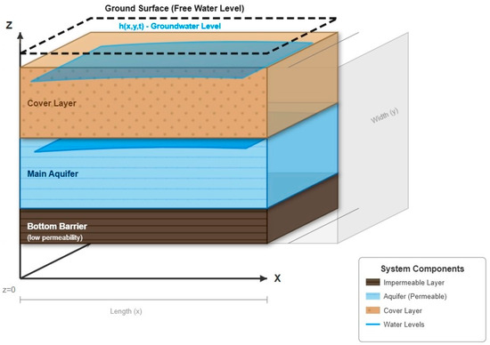
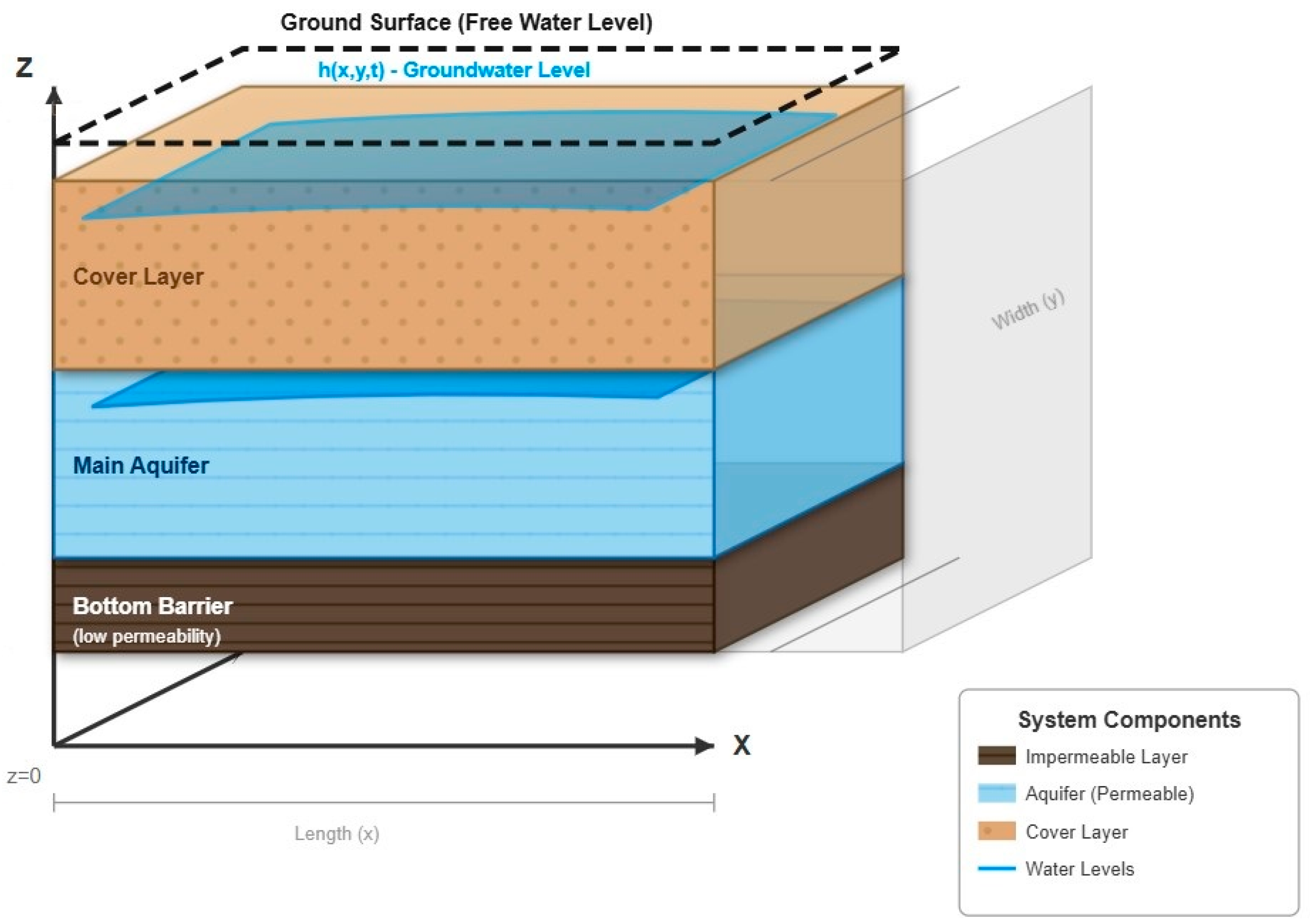
The spatial domain G is defined as a rectangular region with horizontal dimensions $L_x$ and $L_y$ in the $x$ and $y$ directions, respectively. The vertical extent encompasses all three layers, with the water table surface forming the upper boundary and the base of the barrier layer constituting the lower boundary. Figure 1 illustrates the conceptual model of the three-layered groundwater system, showing the relative positions of each layer and the primary flow components.

Figure 1. Three-layered groundwater system.

3.1.2. Fundamental Assumptions

The mathematical model is developed under the following fundamental assumptions that balance physical realism with computational tractability:

The Dupuit–Forchheimer approximation applies to horizontal flow in the covering layer, whereby vertical flow components are negligible compared to horizontal components, and the hydraulic gradient equals the slope of the water table [36].

Flow in the main confined aquifer follows Darcy’s law [15] with spatially variable but temporally constant hydraulic conductivity, represented by the transmissivity function

$$T(x,y)=k_p(x,y)\cdot m_p.$$

Vertical flow through the barrier layer occurs under quasi-steady conditions, with the vertical hydraulic gradient assumed constant throughout the layer thickness at any given time. The aquifer materials exhibit elastic storage behavior, characterized by specific yield ${\mu }_v$ in the unconfined covering layer and specific storage coefficients $\mu$ and ${\mu }_p$ in the confined layers.

Water density and viscosity remain constant throughout the domain, eliminating buoyancy effects and allowing the use of hydraulic head as the primary state variable. The principle of mass conservation [7] applies at all scales, with no internal sources or sinks except for explicitly defined wells, drains, or other hydraulic structures.

3.1.3. Governing Equations

Based on these assumptions and applying the principle of mass conservation to each layer, we derive the following system of coupled partial differential equations governing groundwater flow:

$$\left\{\begin{array}{l}{\mu }_v{\displaystyle \frac{\partial h}{\partial t}}={\displaystyle \frac{\partial }{\partial x}}\left(k_{g}h{\displaystyle \frac{\partial h}{\partial x}}\right)+{\displaystyle \frac{\partial }{\partial y}}\left(k_{g}h{\displaystyle \frac{\partial h}{\partial y}}\right)-k_g\left(1-{\displaystyle \frac{H}{h}}\right)+f-W\\ \mu {\displaystyle \frac{\partial H}{\partial t}}={\displaystyle \frac{\partial }{\partial x}}\left(T{\displaystyle \frac{\partial H}{\partial x}}\right)+{\displaystyle \frac{\partial }{\partial y}}\left(T{\displaystyle \frac{\partial H}{\partial y}}\right)+k_g\left(1-{\displaystyle \frac{H}{h}}\right)-k_p{\left.{\displaystyle \frac{\partial u}{\partial z}}\right|}_{z=m_p}\\ {\displaystyle \frac{\partial u}{\partial t}}=a_p{\displaystyle \frac{{\partial }^{2}u}{\partial z^2}}\end{array}\right.$$

(1)

where $x$, $y$, and $z$ are spatial coordinates (m), $(x,y,z)\in G$, $G$ is filtration domain, $t$ is time (days), $h(x,y,t)$ is groundwater level from the free surface to the upper boundary of the main aquifer (m), $H(x,y,t)$ is pressure in the main aquifer (m), $u(x,y,z,t)$ is pressure at the boundary of the weakly permeable layer (m), $k_g,k,k_p,m_v,m,m_p$ are filtration coefficients (m/day) and thicknesses (m) of the covering layer, main layer, and weakly permeable layer, respectively, $T(x,y)=mk$ is hydraulic conductivity function of the main aquifer (m²/day), $a_p={\displaystyle \frac{k_p{m}_p}{{\mu }_p^{\ast }}}$ is piezoconductivity coefficient of the low-permeability layer (m²/day), ${\mu }_v$ is water yield coefficient or deficit in saturation degree of the covering layer (-), $\mu ,{\mu }_p$ are water release coefficients (-), $\xi ,\eta$ are permeability coefficients at the boundaries (for example, riverbed permeability) (m/day), and $f$ is infiltration function (m/day). The following ratio is used to calculate precipitation [41,42,43]:

$$f=f_0+\Delta f\sin wt,$$

where $f_0$ is average monthly variation in precipitation amount, $\Delta f$ is annual variation in precipitation amount, and $w$ is cyclic frequency of monthly variation (1/day).

For evaporation, we apply the M.M. Krylov-S.F. Averyanov law [17]. We consider the horizontal components of the filtration velocity in the covering layer. Evaporation is accounted for according to the Krylov–Averyanov theory, i.e., its intensity depends on the depth of the groundwater level. The form of this dependence is adopted as follows [17]:

$$W=\left\{\begin{array}{l}{W}_S{\left(1-{\displaystyle \frac{h}{h_{kr}}}\right)}^n, h>h_{kr}\\ 0, h\le h_{kr}\end{array}\right.$$

(2)

$W$—evaporation intensity at groundwater depth $h$ (m/day); $W_S$—evaporation intensity from the soil surface under conditions of very high groundwater level (can be assumed approximately equal to evaporation from the water surface); $n$—parameter; $h_{kr}$—critical groundwater level. According to this, if the groundwater level is above the evaporation threshold, i.e., the critical level, evaporation occurs based on the above law. If the level does not exceed the critical level, evaporation is not observed.

The following formula was used to calculate the periodic changes in evaporation [44]:

$$W_S=W_0+\Delta W\sin wt$$

where $W_0$—average monthly change in evaporation; $\Delta W$—annual amplitude of evaporation change; $w$—cyclic frequency of monthly change.

3.1.4. Boundary and Initial Conditions

The mathematical problem requires specification of appropriate boundary conditions at the domain boundaries and initial conditions throughout the domain. At the lateral boundaries, we prescribe mixed-type conditions that account for variable permeability:

• Initial conditions:

$${\left.h\right|}_{t=0}=h_0,{\left.H\right|}_{t=0}=H_0,{\left.u\right|}_{t=0}=u_0.$$

(3)

Boundary conditions:

$$\begin{array}{l}{\left.k_{g}h{\displaystyle \frac{\partial h}{\partial x}}\right|}_{x=0}=-\xi (h-h_A); {\left.k_{g}h{\displaystyle \frac{\partial h}{\partial x}}\right|}_{x=L}=\xi (h-h_B);\\ {\left.k_{g}h{\displaystyle \frac{\partial h}{\partial y}}\right|}_{y=0}=-\xi (h-h_C); k_{g}h{\left.{\displaystyle \frac{\partial h}{\partial y}}\right|}_{y=L}=\xi (h-h_D);\end{array}$$

(4)

$$\begin{array}{l}{\left.T{\displaystyle \frac{\partial H}{\partial x}}\right|}_{x=0}=-\eta (H-H_A); {\left.T{\displaystyle \frac{\partial H}{\partial x}}\right|}_{x=L}=\eta (H-H_B);\\ {\left.T{\displaystyle \frac{\partial H}{\partial y}}\right|}_{y=0}=-\eta (H-H_C); {\left.T{\displaystyle \frac{\partial H}{\partial y}}\right|}_{y=L}=\eta (H-H_D);\end{array}$$

(5)

$${\left.{\displaystyle \frac{\partial u}{\partial z}}\right|}_{z=0}=0.$$

(6)

where $h_0$ is initial groundwater level (m), $h_A,h_B,h_C,h_D$ are groundwater levels at the boundaries (m), $H_0$ is initial pressure in the main aquifer (m), $H_A,H_B,H_C,H_D$ are pressures in the main aquifer at the boundaries (m), and $u_0$ is initial pressure at the boundary of the weakly permeable layer (m).

Equations (4) and (5) represent the four outer boundaries of the computational domain shown in Figure 1, denoted as A, B, C, and D:

• A: Western boundary (x = 0).
• B: Eastern boundary (x = L_x).
• C: Southern boundary (y = 0).
• D: Northern boundary (y = L_y).

A mixed-type condition is applied at each boundary, which expresses the water flow through the boundary in terms of the permeability coefficient $(k_i)$ and the hydraulic head difference. This approach allows modeling of the real interaction between a river, canal, or other water body and the aquifer.

3.2. Solution of the Problem

This problem is solved for the case where n = 2. This selection is based on several scientific principles. The parameter n is an empirical coefficient representing the capillary properties of soil, specifically how the efficiency of moisture uplift changes as the groundwater level decreases. Scientific literature indicates that its value typically ranges from 1 to 4, depending on the soil’s mechanical composition.

• n = 1 (Linear model): This value implies a linear decrease in evaporation intensity as the water table deepens. This approach is often considered an oversimplification for complex natural processes.
• n = 2 (Parabolic model): This value is widely used for medium loamy and sandy loam soils. It reflects a sharper, nonlinear (parabolic) decrease in evaporation intensity as the water level approaches the critical depth. This situation more closely resembles the real physical process that occurs due to the disruption of the capillary system.
• n > 2: These values are typically characteristic of heavy, clayey soils, which can draw moisture from considerable depths due to strong capillarity. After the water level passes a certain threshold, evaporation stops very abruptly.

The alluvial deposits of the Zarafshan River valley, which are the object of this research, are primarily composed of medium loamy and sandy loam soils. Therefore, choosing the value n = 2 for this area is considered the most physically justified and optimal option. This selection allows the model to more accurately reflect real hydrogeological conditions. In this case, the system of Equation (1) will have the following form:

$$\left\{\begin{array}{l}{\mu }_v{\displaystyle \frac{\partial h}{\partial t}}={\displaystyle \frac{\partial }{\partial x}}\left(k_{g}h{\displaystyle \frac{\partial h}{\partial x}}\right)+{\displaystyle \frac{\partial }{\partial y}}\left(k_{g}h{\displaystyle \frac{\partial h}{\partial y}}\right)-k_g\left(1-{\displaystyle \frac{H}{h}}\right)+f-W_S{\left(1-{\displaystyle \frac{h}{h_{kr}}}\right)}^2\\ \mu {\displaystyle \frac{\partial H}{\partial t}}={\displaystyle \frac{\partial }{\partial x}}\left(T{\displaystyle \frac{\partial H}{\partial x}}\right)+{\displaystyle \frac{\partial }{\partial y}}\left(T{\displaystyle \frac{\partial H}{\partial y}}\right)+k_g\left(1-{\displaystyle \frac{H}{h}}\right)-k_p{\left.{\displaystyle \frac{\partial u}{\partial z}}\right|}_{z=m_p}\\ {\displaystyle \frac{\partial u}{\partial t}}=a_p{\displaystyle \frac{{\partial }^{2}u}{\partial z^2}}\end{array}\right.$$

(7)

To solve the Problem (7), Equations (3)–(6), the equation and its initial and boundary conditions are first converted into dimensionless quantities. For this purpose, the following transformations are used:

$$\begin{array}{l}{h}^{\ast }={\displaystyle \frac{h}{H_{xar}}}; H^{\ast }={\displaystyle \frac{H}{H_{xar}}}; u^{\ast }={\displaystyle \frac{u}{H_{xar}}}; x^{\ast }={\displaystyle \frac{x}{L}}; y^{\ast }={\displaystyle \frac{y}{L}}; z^{\ast }={\displaystyle \frac{z}{m_p}}; T^{\ast }={\displaystyle \frac{T}{T_0}}; k_g^{\ast }={\displaystyle \frac{k_g}{k_0}};\\ \tau ={\displaystyle \frac{T_0}{\mu L^2}}t; h_{kr}^{\ast }={\displaystyle \frac{h_{kr}}{H_{xar}}};k_p^{\ast }={\displaystyle \frac{k_p}{k_0}};{\xi }^{\ast }={\displaystyle \frac{\xi }{{\xi }_0}};{\eta }^{\ast }={\displaystyle \frac{\eta }{{\eta }_0}}\end{array}$$

where $H_{chr}, T_0, k_0, {\xi }_0, {\eta }_0$—pressure function, filtration permeability, filtration coefficient and some characteristic values of the permeability coefficients at the boundaries; $L$—maximum length of the region $G$ in plan view.

The system of equations in Equation (7) is transformed into dimensionless form. For this purpose, each equation is converted to a separate dimensionless form. The dimensionless form of the first equation in the system of equations:

$${\mu }_v{\displaystyle \frac{\partial h^{\ast }}{\partial \tau }}=\alpha \left[{\displaystyle \frac{\partial }{\partial x^{\ast }}}\left(k_g^{\ast }{h}^{\ast }{\displaystyle \frac{\partial h^{\ast }}{\partial x^{\ast }}}\right)+{\displaystyle \frac{\partial }{\partial y^{\ast }}}\left(k_g^{\ast }{h}^{\ast }{\displaystyle \frac{\partial h^{\ast }}{\partial y^{\ast }}}\right)\right]-\beta k_g^{\ast }\left(1-{\displaystyle \frac{H^{\ast }}{h^{\ast }}}\right)+f^{\ast }-W_s^{\ast }{\left(1-{\displaystyle \frac{h^{\ast }}{h_{kr}^{\ast }}}\right)}^2$$

where $f^{\ast }={\displaystyle \frac{\mu L^2}{T_0{H}_{chr}}}f$, $W_s^{\ast }={\displaystyle \frac{\mu L^2}{T_0{H}_{chr}}}{W}_s$.

• The dimensionless form of the second equation is:

  $${\displaystyle \frac{\partial H^{\ast }}{\partial \tau }}={\displaystyle \frac{\partial }{\partial x^{\ast }}}\left(T^{\ast }{\displaystyle \frac{\partial H^{\ast }}{\partial x^{\ast }}}\right)+{\displaystyle \frac{\partial }{\partial y^{\ast }}}\left(T^{\ast }{\displaystyle \frac{\partial H^{\ast }}{\partial y^{\ast }}}\right)+\gamma k_g^{\ast }\left(1-{\displaystyle \frac{H^{\ast }}{h^{\ast }}}\right)-\lambda k_p^{\ast }{\left.{\displaystyle \frac{\partial u^{\ast }}{\partial z^{\ast }}}\right|}_{z^{\ast }=1}$$

  The dimensionless form of the third equation is:

  $${\displaystyle \frac{\partial u\ast }{\partial \tau }}=\rho {\displaystyle \frac{{\partial }^2{u}^{\ast }}{\partial {(z^{\ast })}^2}}$$

  To obtain a simplified form, we remove the “*” symbol from the equations, and as a result, the dimensionless form of the system of equations in Equation (7) will be:

  $$\left\{\begin{array}{l}{\mu }_v{\displaystyle \frac{\partial h}{\partial \tau }}=\alpha \left[{\displaystyle \frac{\partial }{\partial x}}\left(k_{g}h{\displaystyle \frac{\partial h}{\partial x}}\right)+{\displaystyle \frac{\partial }{\partial y}}\left(k_{g}h{\displaystyle \frac{\partial h}{\partial y}}\right)\right]-\beta k_g\left(1-{\displaystyle \frac{H}{h}}\right)+f-W_s{\left(1-{\displaystyle \frac{h}{h_{kr}}}\right)}^2\\ {\displaystyle \frac{\partial H}{\partial \tau }}={\displaystyle \frac{\partial }{\partial x}}\left(T{\displaystyle \frac{\partial H}{\partial x}}\right)+{\displaystyle \frac{\partial }{\partial y}}\left(T{\displaystyle \frac{\partial H}{\partial y}}\right)+\gamma k_g\left(1-{\displaystyle \frac{H}{h}}\right)-\lambda k_p{\left.{\displaystyle \frac{\partial u}{\partial z}}\right|}_{z=1}\\ {\displaystyle \frac{\partial u}{\partial \tau }}=\rho {\displaystyle \frac{{\partial }^{2}u}{\partial z^2}}\end{array}\right.$$

  (8)

  where $\alpha ={\displaystyle \frac{\mu k_0{H}_{chr}}{T_0}}$, $\beta ={\displaystyle \frac{\mu k_0{L}^2}{T_0{H}_{chr}}}$, $\gamma ={\displaystyle \frac{k_0{L}^2}{T_0{H}_{chr}}}$, $\lambda ={\displaystyle \frac{k_0{L}^2}{T_0{m}_p}}$, and $\rho ={\displaystyle \frac{a_p\mu L^2}{T_0{m}_p^2}}$.

The initial and boundary conditions are also converted to dimensionless form: ${\left.h^{\ast }\right|}_{\tau =0}=h_0^{\ast }, {\left.H^{\ast }\right|}_{\tau =0}=H_0^{\ast }, {\left.u^{\ast }\right|}_{\tau =0}=u_0^{\ast }.$

$$\begin{array}{l}{\left.\sigma k_g^{\ast }{h}^{\ast }{\displaystyle \frac{\partial h^{\ast }}{\partial x^{\ast }}}\right|}_{x^{\ast }=0}=-{\xi }^{\ast }(h^{\ast }-h_A^{\ast }); {\left.\sigma k_g^{\ast }{h}^{\ast }{\displaystyle \frac{\partial h^{\ast }}{\partial x^{\ast }}}\right|}_{x^{\ast }=1}={\xi }^{\ast }(h^{\ast }-h_B^{\ast });\\ {\left.\sigma k_g^{\ast }{h}^{\ast }{\displaystyle \frac{\partial h^{\ast }}{\partial y^{\ast }}}\right|}_{y^{\ast }=0}=-{\xi }^{\ast }(h^{\ast }-h_C^{\ast }); {\left.\sigma k_g^{\ast }{h}^{\ast }{\displaystyle \frac{\partial h^{\ast }}{\partial y^{\ast }}}\right|}_{y^{\ast }=1}={\xi }^{\ast }(h^{\ast }-h_D^{\ast });\end{array}$$

$$\begin{array}{l}\theta {\left.T^{\ast }{\displaystyle \frac{\partial H^{\ast }}{\partial x^{\ast }}}\right|}_{x^{\ast }=0}=-{\eta }^{\ast }(H^{\ast }-H_A^{\ast }); \theta {\left.T^{\ast }{\displaystyle \frac{\partial H^{\ast }}{\partial x^{\ast }}}\right|}_{x^{\ast }=1}={\eta }^{\ast }(H^{\ast }-H_B^{\ast });\\ \theta {\left.T^{\ast }{\displaystyle \frac{\partial H^{\ast }}{\partial y^{\ast }}}\right|}_{y^{\ast }=0}=-{\eta }^{\ast }(H^{\ast }-H_C^{\ast }); \theta {\left.T^{\ast }{\displaystyle \frac{\partial H^{\ast }}{\partial y^{\ast }}}\right|}_{y^{\ast }=1}={\eta }^{\ast }(H^{\ast }-H_D^{\ast });\end{array}$$

$${\left.{\displaystyle \frac{\partial u^{\ast }}{\partial z^{\ast }}}\right|}_{z^{\ast }=0}=0.$$

where $\sigma ={\displaystyle \frac{k_0{H}_{chr}}{{\xi }_{0}L}}$ and $\theta ={\displaystyle \frac{k_0{H}_{chr}}{{\eta }_{0}L}}$.

• For convenience, we remove the “*” symbol from the initial and boundary conditions:

  $${\left.h\right|}_{\tau =0}=h_0,{\left.H\right|}_{\tau =0}=H_0,{\left.u\right|}_{\tau =0}=u_0.$$

  (9)

  $$\begin{array}{l}{\left.\sigma k_{g}h{\displaystyle \frac{\partial h}{\partial x}}\right|}_{x=0}=-\xi (h-h_A); {\left.\sigma k_{g}h{\displaystyle \frac{\partial h}{\partial x}}\right|}_{x=1}=\xi (h-h_B);\\ {\left.\sigma k_{g}h{\displaystyle \frac{\partial h}{\partial y}}\right|}_{y=0}=-\xi (h-h_C); {\left.\sigma k_{g}h{\displaystyle \frac{\partial h}{\partial y}}\right|}_{y=1}=\xi (h-h_D);\end{array}$$

  (10)

  $$\begin{array}{l}\theta {\left.T{\displaystyle \frac{\partial H}{\partial x}}\right|}_{x=0}=-\eta (H-H_A); \theta {\left.T{\displaystyle \frac{\partial H}{\partial x}}\right|}_{x=1}=\eta (H-H_B);\\ \theta {\left.T{\displaystyle \frac{\partial H}{\partial y}}\right|}_{y=0}=-\eta (H-H_C); \theta {\left.T{\displaystyle \frac{\partial H}{\partial y}}\right|}_{y=1}=\eta (H-H_D);\end{array}$$

  (11)

  $${\left.{\displaystyle \frac{\partial u}{\partial z}}\right|}_{z=0}=0.$$

  (12)

  Let’s rewrite the system of equations in Equation (8):

  $$\left\{\begin{array}{l}{\displaystyle \frac{{\mu }_v}{\tilde{h}}}{\displaystyle \frac{\partial h^2}{\partial \tau }}={\displaystyle \frac{\alpha }{2}}\left[{\displaystyle \frac{\partial }{\partial x}}\left(k_g{\displaystyle \frac{\partial h^2}{\partial x}}\right)+{\displaystyle \frac{\partial }{\partial y}}\left(k_g{\displaystyle \frac{\partial h^2}{\partial y}}\right)\right]-\beta k_g\left(1-{\displaystyle \frac{H}{h}}\right)+f-W_s+2W_s{\displaystyle \frac{h}{h_{cr}}}-W_s{\displaystyle \frac{h^2}{h_{cr}^2}}\\ {\displaystyle \frac{\partial H}{\partial \tau }}={\displaystyle \frac{\partial }{\partial x}}\left(T{\displaystyle \frac{\partial H}{\partial x}}\right)+{\displaystyle \frac{\partial }{\partial y}}\left(T{\displaystyle \frac{\partial H}{\partial y}}\right)+\gamma k_g\left(1-{\displaystyle \frac{H}{h}}\right)-\lambda k_p{\displaystyle \frac{\partial u(x,y,1)}{\partial z}}\\ {\displaystyle \frac{\partial u}{\partial \tau }}=\rho {\displaystyle \frac{{\partial }^{2}u}{\partial z^2}}\end{array}\right.$$

  (13)

  where $\tilde{h}$ represents the value from the previous iteration during the calculation process. The boundary conditions are also rewritten as follows:

  $$\begin{array}{l}{\left.{\displaystyle \frac{\sigma k_g}{2}}\cdot {\displaystyle \frac{\partial h^2}{\partial x}}\right|}_{x=0}=-\xi (h-h_A); {\left.{\displaystyle \frac{\sigma k_g}{2}}\cdot {\displaystyle \frac{\partial h^2}{\partial x}}\right|}_{x=1}=\xi (h-h_B);\\ {\left.{\displaystyle \frac{\sigma k_g}{2}}\cdot {\displaystyle \frac{\partial h^2}{\partial y}}\right|}_{y=0}=-\xi (h-h_C); {\left.{\displaystyle \frac{\sigma k_g}{2}}\cdot {\displaystyle \frac{\partial h^2}{\partial y}}\right|}_{y=1}=\xi (h-h_D);\end{array}$$

  (14)

  $$\begin{array}{l}\theta {\left.T{\displaystyle \frac{\partial H}{\partial x}}\right|}_{x=0}=-\eta (H-H_A); \theta {\left.T{\displaystyle \frac{\partial H}{\partial x}}\right|}_{x=1}=\eta (H-H_B);\\ \theta {\left.T{\displaystyle \frac{\partial H}{\partial y}}\right|}_{y=0}=-\eta (H-H_C); \theta {\left.T{\displaystyle \frac{\partial H}{\partial y}}\right|}_{y=1}=\eta (H-H_D);\end{array}$$

  (15)

  $${\left.{\displaystyle \frac{\partial u}{\partial z}}\right|}_{z=0}=0.$$

  (16)

Numerical Solution of the Problem

To solve the problem numerically, we create a grid on some plane G. Such a grid is created in the form:

$${\Omega }_{\Delta x,\Delta y,\Delta t}=\left\{x_i=i\Delta x,i=\overline{0,N_x};y_j=j\Delta y,j=\overline{0,N_y};t_n=n\Delta t,n=\overline{0,N_t}\right\}.$$

Equation (13) is then numerically solved using the alternating directions method [41,42,43]. To accomplish this, we first apply a scheme that is implicit in the x-direction and explicit in the y-direction and then discretize Equation (13):

$$\begin{array}{l}{\displaystyle \frac{{(h_{i,j}^{n+\frac{1}{2}})}^2-{(h_{i,j}^n)}^2}{0.5\Delta t}}={\displaystyle \frac{\alpha h_{i,j}^n}{{\mu }_v}}{\left[{\displaystyle \frac{\partial }{\partial x}}\left(k{\displaystyle \frac{\partial h^2}{\partial x}}\right)\right]}_{i,j}^{n+{\displaystyle \frac{1}{2}}}+{\displaystyle \frac{\alpha h_{i,j}^n}{{\mu }_v}}{\left[{\displaystyle \frac{\partial }{\partial y}}\left(k{\displaystyle \frac{\partial h^2}{\partial y}}\right)\right]}_{i,j}^n-\\ -{\displaystyle \frac{h_{i,j}^n\beta k_g}{{\mu }_v}}\left(1-{\displaystyle \frac{H_{i,j}}{h_{i,j}}}\right)+{\displaystyle \frac{h_{i,j}^n{f}_{i,j}}{{\mu }_v}}-{\displaystyle \frac{\Delta t{h}_{i,j}^n{W}_{i,j}}{{\mu }_v}}{\left(1-{\displaystyle \frac{h_{i,j}^n}{h_{kr}}}\right)}^2\end{array}$$

(17)

By introducing the notations $\chi ={\displaystyle \frac{\alpha \Delta t}{2{\mu }_v}}$ and

• $F_{i,j}=-{\displaystyle \frac{h_{i,j}^n\beta k_g}{{\mu }_v}}\left(1-{\displaystyle \frac{H_{i,j}}{h_{i,j}}}\right)+{\displaystyle \frac{h_{i,j}^n{f}_{i,j}}{{\mu }_v}}-{\displaystyle \frac{\Delta t{h}_{i,j}^n{W}_{i,j}}{{\mu }_v}}{\left(1-{\displaystyle \frac{h_{i,j}^n}{h_{kr}}}\right)}^2$, Equation (17) is written in the following form:

  $${(h_{i,j}^{n+{\displaystyle \frac{1}{2}}})}^2={(h_{i,j}^n)}^2+\chi h_{i,j}^n{\left[{\displaystyle \frac{\partial }{\partial x}}\left(k{\displaystyle \frac{\partial h^2}{\partial x}}\right)\right]}_{i,j}^{n+{\displaystyle \frac{1}{2}}}+\chi h_{i,j}^n{\left[{\displaystyle \frac{\partial }{\partial y}}\left(k{\displaystyle \frac{\partial h^2}{\partial y}}\right)\right]}_{i,j}^n+F_{i,j}$$

  (18)

  Along the time layer, the implicit half-step in the $x$ direction is discretized as follows:

  $${\left[{\displaystyle \frac{\partial }{\partial x}}\left(k{\displaystyle \frac{\partial h^2}{\partial x}}\right)\right]}_{i,j}^{n+{\displaystyle \frac{1}{2}}}\approx {\displaystyle \frac{1}{\Delta x^2}}\left[\begin{array}{l}{k}_{i+{\displaystyle \frac{1}{2}},j}{(h_{i+1,j}^{n+{\displaystyle \frac{1}{2}}})}^2-(k_{i+{\displaystyle \frac{1}{2}},j}+k_{i-{\displaystyle \frac{1}{2}},j}){(h_{i,j}^{n+{\displaystyle \frac{1}{2}}})}^2+\\ +k_{i-{\displaystyle \frac{1}{2}},j}{(h_{i-1,j}^{n+{\displaystyle \frac{1}{2}}})}^2\end{array}\right]$$

  (19)

  In Equation (19), a quasi-linear substitution is applied for the unknowns. In finite-difference schemes, for unknown terms, substitution is performed using the quasi-linear transformation ${\tilde{h}}_{i,j}=h_{i,j}^n$ based on the formula $h^2\approx 2\tilde{h}h-{\tilde{h}}^2$ [43,44]:

  $$\begin{array}{c}{\left[{\displaystyle \frac{\partial }{\partial x}}\left(k{\displaystyle \frac{\partial h^2}{\partial x}}\right)\right]}_{i,j}^{n+{\displaystyle \frac{1}{2}}}\approx {\displaystyle \frac{2k_{i+\frac{1}{2},j}{h}_{i+1,j}^n}{\Delta x^2}}{h}_{i+1,j}^{n+{\displaystyle \frac{1}{2}}}-\\ -{\displaystyle \frac{2(k_{i+\frac{1}{2},j}+k_{i-\frac{1}{2},j})h_{i,j}^n}{\Delta x^2}}{h}_{i,j}^{n+{\displaystyle \frac{1}{2}}}+{\displaystyle \frac{2k_{i-\frac{1}{2},j}{h}_{i-1,j}^n}{\Delta x^2}}{h}_{i-1,j}^{n+{\displaystyle \frac{1}{2}}}-\\ -{\displaystyle \frac{1}{\Delta x^2}}\left[k_{i+{\displaystyle \frac{1}{2}},j}{(h_{i+1,j}^n)}^2-(k_{i+{\displaystyle \frac{1}{2}},j}+k_{i-{\displaystyle \frac{1}{2}},j}){(h_{i,j}^n)}^2+k_{i-{\displaystyle \frac{1}{2}},j}{(h_{i-1,j}^n)}^2\right]\end{array}$$

  (20)

  where $k_{i+{\displaystyle \frac{1}{2}},j}\approx {\displaystyle \frac{k_{i+1,j}+k_{i,j}}{2}},k_{i-{\displaystyle \frac{1}{2}},j}\approx {\displaystyle \frac{k_{i,j}+k_{i-1,j}}{2}}$.
  The discrete form of the differential of Equation (17) along the $y$-axis is as follows:

  $${\left[{\displaystyle \frac{\partial }{\partial y}}\left(k{\displaystyle \frac{\partial h^2}{\partial y}}\right)\right]}_{i,j}^n\approx {\displaystyle \frac{1}{\Delta y^2}}\left[\begin{array}{l}{k}_{i,j+{\displaystyle \frac{1}{2}}}{(h_{i,j+1}^n)}^2-(k_{i,j+{\displaystyle \frac{1}{2}}}+k_{i,j-{\displaystyle \frac{1}{2}}}){(h_{i,j}^n)}^2+\\ +k_{i,j-{\displaystyle \frac{1}{2}}}{(h_{i,j-1}^n)}^2\end{array}\right]$$

  (21)

  where $k_{i,j+{\displaystyle \frac{1}{2}}}\approx {\displaystyle \frac{k_{i,j+1}+k_{i,j}}{2}},k_{i,j-{\displaystyle \frac{1}{2}}}\approx {\displaystyle \frac{k_{i,j}+k_{i,j-1}}{2}}$.
  Based on Equations (20) and (21), Equation (17) takes the following form:

  $$\begin{array}{l}{h}_{i,j}^{n+{\displaystyle \frac{1}{2}}}=h_{i,j}^n+\\ +{\displaystyle \frac{\chi }{2}}\left[{\displaystyle \frac{2k_{i+\frac{1}{2},j}{h}_{i+1,j}^n}{\Delta x^2}}{h}_{i+1,j}^{n+{\displaystyle \frac{1}{2}}}-{\displaystyle \frac{2(k_{i+\frac{1}{2},j}+k_{i-\frac{1}{2},j})h_{i,j}^n}{\Delta x^2}}{h}_{i,j}^{n+{\displaystyle \frac{1}{2}}}+{\displaystyle \frac{2k_{i-\frac{1}{2},j}{h}_{i-1,j}^n}{\Delta x^2}}{h}_{i-1,j}^{n+{\displaystyle \frac{1}{2}}}\right]-\\ -{\displaystyle \frac{\chi }{2\Delta x^2}}\left[k_{i+{\displaystyle \frac{1}{2}},j}{(h_{i+1,j}^n)}^2-(k_{i+{\displaystyle \frac{1}{2}},j}+k_{i-{\displaystyle \frac{1}{2}},j}){(h_{i,j}^n)}^2+k_{i-{\displaystyle \frac{1}{2}},j}{(h_{i-1,j}^n)}^2\right]+\\ +{\displaystyle \frac{\chi }{2\Delta y^2}}\left[k_{i,j+{\displaystyle \frac{1}{2}}}{(h_{i,j+1}^n)}^2-(k_{i,j+{\displaystyle \frac{1}{2}}}+k_{i,j-{\displaystyle \frac{1}{2}}}){(h_{i,j}^n)}^2+k_{i,j-{\displaystyle \frac{1}{2}}}{(h_{i,j-1}^n)}^2\right]+\\ +F_{i,j}\end{array}$$

  (22)

  Based on transformations of Equation (22), a system of three-point equations is constructed:

  $$\begin{array}{c}-{\displaystyle \frac{\chi k_{i-\frac{1}{2},j}{h}_{i-1,j}^n}{\Delta x^2}}{h}_{i-1,j}^{n+{\displaystyle \frac{1}{2}}}+\left(1+{\displaystyle \frac{\chi (k_{i+\frac{1}{2},j}+k_{i-\frac{1}{2},j})h_{i,j}^n}{\Delta x^2}}\right)h_{i,j}^{n+{\displaystyle \frac{1}{2}}}-{\displaystyle \frac{\chi k_{i+\frac{1}{2},j}{h}_{i+1,j}^n}{\Delta x^2}}{h}_{i+1,j}^{n+{\displaystyle \frac{1}{2}}}=\\ =h_{i,j}^n-{\displaystyle \frac{\chi }{2\Delta x^2}}\left[k_{i+{\displaystyle \frac{1}{2}},j}{(h_{i+1,j}^n)}^2-(k_{i+{\displaystyle \frac{1}{2}},j}+k_{i-{\displaystyle \frac{1}{2}},j}){(h_{i,j}^n)}^2+k_{i-{\displaystyle \frac{1}{2}},j}{(h_{i-1,j}^n)}^2\right]+\\ +{\displaystyle \frac{\chi }{2\Delta y^2}}\left[k_{i,j+{\displaystyle \frac{1}{2}}}{(h_{i,j+1}^n)}^2-(k_{i,j+{\displaystyle \frac{1}{2}}}+k_{i,j-{\displaystyle \frac{1}{2}}}){(h_{i,j}^n)}^2+k_{i,j-{\displaystyle \frac{1}{2}}}{(h_{i,j-1}^n)}^2\right]+F_{i,j}\end{array}$$

  (23)

  For convenience in solving using the Thomas algorithm, the system of equations in Equation (22) is written in the following form:

  $$a_i{h}_{i-1,j}^{n+{\displaystyle \frac{1}{2}}}-c_i{h}_{i,j}^{n+{\displaystyle \frac{1}{2}}}+b_i{h}_{i+1,j}^{n+{\displaystyle \frac{1}{2}}}=-d_i$$

  (24)

  where

  $$\begin{array}{l}{a}_i=-{\displaystyle \frac{\chi k_{i-\frac{1}{2},j}{h}_{i-1,j}^n}{\Delta x^2}},c_i=-\left(1+{\displaystyle \frac{\chi (k_{i+\frac{1}{2},j}+k_{i-\frac{1}{2},j})h_{i,j}^n}{\Delta x^2}}\right),b_i=-{\displaystyle \frac{\chi k_{i+\frac{1}{2},j}{h}_{i+1,j}^n}{\Delta x^2}},\\ d_i=-h_{i,j}^n+{\displaystyle \frac{\chi }{2\Delta x^2}}\left[k_{i+{\displaystyle \frac{1}{2}},j}{(h_{i+1,j}^n)}^2-(k_{i+{\displaystyle \frac{1}{2}},j}+k_{i-{\displaystyle \frac{1}{2}},j}){(h_{i,j}^n)}^2+k_{i-{\displaystyle \frac{1}{2}},j}{(h_{i-1,j}^n)}^2\right]-\\ -{\displaystyle \frac{\chi }{2\Delta y^2}}\left[k_{i,j+{\displaystyle \frac{1}{2}}}{(h_{i,j+1}^n)}^2-(k_{i,j+{\displaystyle \frac{1}{2}}}+k_{i,j-{\displaystyle \frac{1}{2}}}){(h_{i,j}^n)}^2+k_{i,j-{\displaystyle \frac{1}{2}}}{(h_{i,j-1}^n)}^2\right]-F_{i,j}.\end{array}$$

  The boundary conditions (Equation (13)) are discretized and written together with the main equation in the form of a system of equations:

  $$\left\{\begin{array}{c}(1-6p_1{h}_{0,j}^n)h_{0,j}^{n+{\displaystyle \frac{1}{2}}}+8p_1{h}_{1,j}^n{h}_{1,j}^{n+{\displaystyle \frac{1}{2}}}-2p_1{h}_{2,j}^n{h}_{2,j}^{n+{\displaystyle \frac{1}{2}}}=\\ =-p_1\left[3{(h_{0,j}^n)}^2-4{(h_{1,j}^n)}^2+{(h_{2,j}^n)}^2\right]+h_A\\ a_i{h}_{i-1,j}^{n+{\displaystyle \frac{1}{2}}}-c_i{h}_{i,j}^{n+{\displaystyle \frac{1}{2}}}+b_i{h}_{i+1,j}^{n+{\displaystyle \frac{1}{2}}}=-d_i\\ (6p_1{h}_{N_x,j}^n-1)h_{N_x,j}^{n+{\displaystyle \frac{1}{2}}}-8p_1{h}_{N_x-1,j}^n{h}_{N_x-1,j}^{n+{\displaystyle \frac{1}{2}}}+2p_1{h}_{N_x-2,j}^n{h}_{N_x-2,j}^{n+{\displaystyle \frac{1}{2}}}=\\ =-p_1\left[-3{(h_{N_x,j}^n)}^2+4{(h_{N_x-1,j}^n)}^2-{(h_{N_x-2,j}^n)}^2\right]-h_B\end{array}\right.$$

  (25)

  where $p_1={\displaystyle \frac{\sigma k_g}{4\xi \Delta x}}$.

Boundaries in the y-direction are used to calculate a specific vector on the right side of the system. Here, the “Fictitious node” method is applied. For the lower boundary (j = 0): we first write the condition for the known n-th time layer. We replace ${\displaystyle \frac{\partial h^2}{\partial y}}$ with the central difference around j = 0: ${\displaystyle \frac{{(h_{i,1}^n)}^2-{(h_{i,-1}^n)}^2}{2\Delta y}}$. From the resulting equation, we find the value of the fictitious node ${(h_{i,-1}^n)}^2$ using $h_{i,1}^n$ and $h_{i,0}^n$. The calculated fictitious node value is used to compute the right-hand side vector $d_i$ for the row j = 0 of the main equation. Then, at the upper boundary (j = N_y), we write the condition for the n-th time layer. We replace ${\displaystyle \frac{\partial h^2}{\partial y}}$ with the central difference around j = N_y: ${\displaystyle \frac{{(h_{i,N_y+1}^n)}^2-{(h_{i,N_y-1}^n)}^2}{2\Delta y}}$. We determine the fictitious node ${(h_{i,N_y+1}^n)}^2$ using $h_{i,N_y}^n$ and $h_{i,N_y-1}^n$. The obtained fictitious node value is used to calculate the right-hand side vector $d_i$ for the row j = N_y of the main equation.

We seek the solution of the system of equations in Equation (24) in the form $h_{i,j}^{n+{\displaystyle \frac{1}{2}}}=h_{i+1,j}^{n+{\displaystyle \frac{1}{2}}}{A}_{i+1}+B_{i+1},i=0,1,2,\dots ,N_x-1$ according to Thomas’s algorithm. The $A_{i+1},B_{i+1}$ terms are determined using recurrent formulas $A_{i+1}={\displaystyle \frac{b_i}{c_i-a_i{A}_i}},$ $B_{i+1}={\displaystyle \frac{d_i+a_i{B}_i}{c_i-a_i{A}_i}},$ $i=1,2,\dots ,N_x-1$.

The process of checking convergence in the above calculations involves comparing the solution obtained in the current iteration with the solution from the previous iteration. This comparison is carried out by estimating the maximum absolute difference between consecutive iterative values at all spatial points and is expressed as $\left|{\left(h_{i,j}^{n+{\displaystyle \frac{1}{2}}}\right)}^{\left(s+1\right)}-{\left(h_{i,j}^{n+{\displaystyle \frac{1}{2}}}\right)}^{\left(s\right)}\right|<\epsilon$. Here, ε is a predetermined convergence threshold, typically set to a small value such as 10⁻⁵. When the convergence criterion is met, the iterative process for the current j-th horizontal line is considered complete. At this point, the solution $h_{i,j}^{n+{\displaystyle \frac{1}{2}}}$ is set equal to the final iterative value $h_{i,j}^{(s+1)}$ and the algorithm proceeds to process the next horizontal line with index j + 1. If the convergence criterion is not satisfied, the current solution estimate is updated by setting $h^{(s)}$ equal to $h^{(s+1)}$, and the calculation process returns to recalculating the coefficients of the tridiagonal matrix before performing another iteration. This iterative process continues until the first half-step of the Alternating Direction Implicit (ADI) method is completed for each horizontal line.

As the next step, Equation (18) is written in the form of a system of three-point equations, using a computational scheme that is implicit in the y-direction and explicit in the x-direction:

$$a_j{h}_{i,j-1}^{n+1}-c_j{h}_{i,j}^{n+1}+b_j{h}_{i,j+1}^{n+1}=-d_j$$

(26)

where

$$a_j=-{\displaystyle \frac{\chi k_{i,j-\frac{1}{2}}{h}_{i,j-1}^{n+\frac{1}{2}}}{\Delta y^2}}, c_j=-\left(1+{\displaystyle \frac{\chi (k_{i,j+\frac{1}{2}}+k_{i,j-\frac{1}{2}})h_{i,j}^{n+\frac{1}{2}}}{\Delta y^2}}\right),b_j=-{\displaystyle \frac{\chi k_{i,j+\frac{1}{2}}{h}_{i,j+1}^{n+\frac{1}{2}}}{\Delta y^2}},$$

$$\begin{array}{l}{d}_j=-h_{i,j}^{n+{\displaystyle \frac{1}{2}}}-{\displaystyle \frac{\chi }{2\Delta x^2}}\left[k_{i+{\displaystyle \frac{1}{2}},j}{(h_{i+1,j}^{n+{\displaystyle \frac{1}{2}}})}^2-(k_{i+{\displaystyle \frac{1}{2}},j}+k_{i-{\displaystyle \frac{1}{2}},j}){(h_{i,j}^{n+{\displaystyle \frac{1}{2}}})}^2+k_{i-{\displaystyle \frac{1}{2}},j}{(h_{i-1,j}^{n+{\displaystyle \frac{1}{2}}})}^2\right]+\\ +{\displaystyle \frac{\chi }{2\Delta y^2}}\left[k_{i,j+{\displaystyle \frac{1}{2}}}{(h_{i,j+1}^{n+{\displaystyle \frac{1}{2}}})}^2-(k_{i,j+{\displaystyle \frac{1}{2}}}+k_{i,j-{\displaystyle \frac{1}{2}}}){(h_{i,j}^{n+{\displaystyle \frac{1}{2}}})}^2+k_{i,j-{\displaystyle \frac{1}{2}}}{(h_{i,j-1}^{n+{\displaystyle \frac{1}{2}}})}^2\right]-F_{i,j}^{n+{\displaystyle \frac{1}{2}}}\end{array}$$

For unknown terms, the quasi-linear substitution ${\tilde{h}}_{i,j}=h_{i,j}^{n+{\displaystyle \frac{1}{2}}}$ is applied.

Using the approximation of the system of equations in Equation (26) and the boundary conditions in Equation (13), the following system of equations is obtained:

$$\left\{\begin{array}{c}(1-6p_2{h}_{i,0}^{n+{\displaystyle \frac{1}{2}}})h_{i,0}^{n+1}+8p_1{h}_{i,1}^{n+{\displaystyle \frac{1}{2}}}{h}_{i,1}^{n+1}-2p_1{h}_{i,2}^{n+{\displaystyle \frac{1}{2}}}{h}_{i,2}^{n+1}=\\ =-p_1\left[3{(h_{i,0}^{n+{\displaystyle \frac{1}{2}}})}^2-4{(h_{i,1}^{n+{\displaystyle \frac{1}{2}}})}^2+{(h_{i,2}^{n+{\displaystyle \frac{1}{2}}})}^2\right]+h_C,\\ a_j{h}_{i,j-1}^{n+1}-c_j{h}_{i,j}^{n+1}+b_j{h}_{i,j+1}^{n+1}=-d_j,\\ (6p_2{h}_{i,N_y}^{n+{\displaystyle \frac{1}{2}}}-1)h_{i,N_y}^{n+1}-8p_2{h}_{i,N_y-1}^{n+{\displaystyle \frac{1}{2}}}{h}_{i,N_y-1}^{n+1}+2p_2{h}_{i,N_y-2}^{n+{\displaystyle \frac{1}{2}}}{h}_{i,N_y-2}^{n+1}=\\ =-p_2\left[-3{(h_{i,N_y}^{n+{\displaystyle \frac{1}{2}}})}^2+4{(h_{i,N_y-1}^{n+{\displaystyle \frac{1}{2}}})}^2-{(h_{i,N_y-2}^{n+{\displaystyle \frac{1}{2}}})}^2\right]-h_D.\end{array}\right.$$

(27)

where $p_2={\displaystyle \frac{\sigma k_g}{4\xi \Delta y}}$.

Similarly to the case in the y-direction described above, the boundaries in the x-direction are used to calculate a specific vector on the right side of the system. Boundary conditions are applied to calculate the vector dj on the right side of the vertical system. The same approach is used for both the left boundary (i = 0) and the right boundary (i = N_x): first, the condition is explicitly expressed for the $n+1/2$ time layer, then the second derivative is approximated using the central difference scheme, and the fictitious node value is determined. The obtained fictitious node values are then used to calculate the vector $d_j$ for the columns i = 0 and i = N_x, respectively.

In the second half-step, the same iterative tridiagonal matrix algorithm is applied as in the first half-step. The main difference is that now the solution process operates along vertical lines in the computational domain and progresses through the j index rather than the i index.

Discretization of the main layer equation. The numerical solution approach for Equation (2) in System (8) is presented below. In the discretization of the second equation, special attention is required for the spatial variability of the transmissivity function T. Values between nodes are calculated using the arithmetic mean. This approach provides a physically accurate flow approximation. Unlike the first equation, the second equation does not require quasi-linearization. The coefficients of the tridiagonal system are directly determined by transmissivity values and vertical flow parameters. This simplifies the calculation process and reduces the number of iterations.

The connection with the lower dense layer is specific to the second equation and is expressed by the term $\lambda k_p{\left.{\displaystyle \frac{\partial u}{\partial z}}\right|}_{z=1}$. This term is related to the solution of the third equation and ensures a complete connection between the layers. The first equation does not have such a connection with the lower layer.

The boundary conditions (Equation (14)) for the second equation have a simpler form than those for the first equation. Due to the absence of nonlinear terms, the boundary conditions are directly incorporated into the tridiagonal system. In the first equation, however, the boundary conditions must also be included in the quasi-linearization process.

In conclusion, the numerical solution of the second equation is simpler than that of the first and requires fewer computational resources. However, both equations are based on the general principles of the ADI method and, when solved together, describe the complete hydrogeological system.

Discretization of the barrier layer equation. In the vertical direction, the barrier layer is divided into N_z layers, and the pressure value is calculated for each layer. The spatial derivative is approximated using a central difference scheme:

$${\displaystyle \frac{{\partial }^{2}u}{\partial z^2}}\approx {\displaystyle \frac{u_{k+1}-2u_k+u_{k-1}}{\Delta z^2}}$$

For time integration, a fully implicit scheme is employed, as this scheme is unconditionally stable and allows for the use of large time steps. The application of the implicit scheme generates a system of tridiagonal equations for each vertical column.

The role of boundary conditions. Boundary conditions are crucial for the third equation. At the upper boundary (z = 1), the pressure is linked to the pressure in the main layer: ${\left.u\right|}_{z=1}=H$. This condition ensures a continuous pressure distribution between the main layer and the barrier layer.

At the lower boundary (z = 0), an impermeable boundary condition (Equation (15)) is typically applied: ${\left.{\displaystyle \frac{\partial u}{\partial z}}\right|}_{z=0}=0$. This condition signifies that there is no water flow beneath the barrier layer. The boundary condition is implemented using the fictitious node method to maintain second-order accuracy.

The solution of the third equation influences the first and second equations through vertical drainage terms. The flow from the main layer to the barrier layer is expressed as $\lambda k_p{\left.{\displaystyle \frac{\partial u}{\partial z}}\right|}_{z=1}$. This term appears in the second equation as a source term and describes the water exchange between the layers.

Unlike the first and second equations, the third equation contains no nonlinear terms. This characteristic eliminates the need for iterative quasi-linearization and allows for the direct solution of a linear system. Consequently, the computational process is accelerated and convergence issues are reduced.

Computational efficiency. Due to the simplicity of the third equation, its numerical solution requires minimal computational resources. Since an independent vertical one-dimensional problem is solved at each point (i, j), the solution of this equation has little impact on the overall computational time of the system. The size of the tridiagonal system depends only on the number of vertical divisions and typically does not exceed 10–20 nodes.

The third equation can be considered in a quasi-stationary approximation, i.e., when the time derivative is small compared to other equations. In this case, the equation becomes elliptic and can be solved directly, further accelerating the calculation process.

The following algorithm presents an optimized parallel implementation using OpenMP technology, designed for efficient execution on modern multi-core personal computers with 4–16 processing cores (Algorithm 1).

Algorithm 1:  GroundwaterFlow_Parallel

// ============= MAIN CONFIGURATION ============= STRUCTURE Config // Grid parameters INTEGER Nx = 200 // Number of points in X direction INTEGER Ny = 200 // Number of points in Y direction INTEGER Nz = 10 // Number of points in Z direction // Parallel computing INTEGER num_threads = GET_SYSTEM_CORES() // Number of system cores // Convergence parameters REAL epsilon = 1 × 10−6 INTEGER max_iter = 100 END STRUCTURE // ============= MAIN PROGRAM ============= PROCEDURE Main() // Configure OpenMP environment CALL omp_set_num_threads(Config.num_threads) // Memory allocation ALLOCATE h[Nx][Ny], h_new[Nx][Ny] ALLOCATE H[Nx][Ny], H_new[Nx][Ny] ALLOCATE u[Nx][Ny][Nz] ALLOCATE W[Nx][Ny], f[Nx][Ny] // Initialize boundary conditions CALL Initialize_Arrays() // Main time loop FOR time_step = 1 TO max_time_steps DO // Calculate evaporation and infiltration in parallel CALL Calculate_Source_Terms_Parallel(time_step) // Apply ADI method CALL ADI_Method_Parallel(time_step) // Solve main aquifer layer equation CALL Solve_Main_Layer_Parallel(time_step) // Solve bottom barrier layer equation CALL Solve_Bottom_Layer_Parallel(time_step) // Update solutions CALL Update_Solutions() END FOR END PROCEDURE // ============= EVAPORATION AND INFILTRATION ============= PROCEDURE Calculate_Source_Terms_Parallel(time_step) current_time = time_step × dt #pragma omp parallel for collapse(2) FOR i = 0 TO Nx−1 DO FOR j = 0 TO Ny(−1 DO // Evaporation calculation IF h[i][j] > hkr THEN W[i][j] = WS * (1 − h[i][j]/hkr)2 * (1 + sin(w*current_time)) ELSE W[i][j] = 0 END IF // Infiltration calculation f[i][j] = f0 + delta_f * sin(w*current_time) END FOR END FOR END PROCEDURE // ============= ADI METHOD − OPTIMIZED ============= PROCEDURE ADI_Method_Parallel(time_step) // Parallel solution in X direction CALL ADI_X_Direction_Parallel() // Wait for all threads to complete #pragma omp barrier // Parallel solution in Y direction CALL ADI_Y_Direction_Parallel() END PROCEDURE // ============= ADI IN X DIRECTION ============= PROCEDURE ADI_X_Direction_Parallel() // Separate thread for each j row #pragma omp parallel for schedule(dynamic) FOR j = 0 TO Ny−1 DO // Local arrays (separate for each thread) REAL a[Nx], b[Nx], c[Nx], d[Nx] REAL h_temp[Nx] converged = FALSE iter = 0 WHILE NOT converged AND iter < max_iter DO iter = iter + 1 // Store previous values FOR i = 0 TO Nx−1 DO h_temp[i] = h[i][j] END FOR // Build tridiagonal system coefficients FOR i = 1 TO Nx−2 DO kg_east = (kg[i][j] + kg[i + 1][j]) / 2.0 kg_west = (kg[i−1][j] + kg[i][j]) / 2.0 // Quasi-linearization IF h_temp[i] > hkr THEN nonlinear = 2.0 * h_temp[i] / (hkr * hkr) ELSE nonlinear = 0 END IF a[i] = −dt * kg_west / (dx * dx) c[i] = −dt * kg_east / (dx * dx) b[i] = 1 + dt * (kg_west + kg_east) / (dx * dx) + dt * nonlinear // Right-hand side d[i] = h[i][j] + dt * (H[i][j] − h[i][j]) + dt * (f[i][j] − W[i][j]) // Add Y-direction diffusion IF j > 0 AND j < Ny−1 THEN kg_north = (kg[i][j] + kg[i][j + 1]) / 2.0 kg_south = (kg[i][j−1] + kg[i][j]) / 2.0 d[i] = d[i] + dt * (kg_north * (h[i][j + 1] − h[i][j]) − kg_south * (h[i][j] - h[i][j−1])) / (dy * dy) END IF END FOR // Boundary conditions a[0] = 0; b[0] = 1; c[0] = 0; d[0] = h_boundary_west(j) a[Nx−1] = 0; b[Nx-1] = 1; c[Nx−1] = 0; d[Nx−1] = h_boundary_east(j) // Apply Thomas algorithm (sequential) CALL Thomas_Solve(a, b, c, d, h_new[0][j], Nx) // Check convergence max_error = 0 FOR i = 0 TO Nx−1 DO error = ABS(h_new[i][j] − h[i][j]) max_error = MAX(max_error, error) h[i][j] = h_new[i][j] END FOR converged = (max_error < epsilon) END WHILE END FOR END PROCEDURE // ============= ADI IN Y DIRECTION ============= PROCEDURE ADI_Y_Direction_Parallel() // Separate thread for each i column #pragma omp parallel for schedule(dynamic) FOR i = 0 TO Nx−1 DO REAL a[Ny], b[Ny], c[Ny], d[Ny] REAL h_temp[Ny] converged = FALSE iter = 0 WHILE NOT converged AND iter < max_iter DO iter = iter + 1 FOR j = 0 TO Ny−1 DO h_temp[j] = h[i][j] END FOR // Tridiagonal system (for Y direction) FOR j = 1 TO Ny-2 DO kg_north = (kg[i][j] + kg[i][j + 1]) / 2.0 kg_south = (kg[i][j−1] + kg[i][j]) / 2.0 IF h_temp[j] > hkr THEN nonlinear = 2.0 * h_temp[j] / (hkr * hkr) ELSE nonlinear = 0 END IF a[j] = −dt * kg_south / (dy * dy) c[j] = −dt * kg_north / (dy * dy) b[j] = 1 + dt * (kg_south + kg_north) / (dy * dy) + dt * nonlinear d[j] = h[i][j] + dt * (H[i][j] − h[i][j]) + dt * (f[i][j] − W[i][j]) END FOR // Boundary conditions a[0] = 0; b[0] = 1; c[0] = 0; d[0] = h_boundary_south(i) a[Ny−1] = 0; b[Ny−1] = 1; c[Ny−1] = 0; d[Ny−1] = h_boundary_north(i) CALL Thomas_Solve(a, b, c, d, h_new[i][0], Ny) // Convergence check max_error = 0 FOR j = 0 TO Ny−1 DO error = ABS(h_new[i][j] − h[i][j]) max_error = MAX(max_error, error) h[i][j] = h_new[i][j] END FOR converged = (max_error < epsilon) END WHILE END FOR END PROCEDURE // ============= MAIN AQUIFER LAYER EQUATION ============= PROCEDURE Solve_Main_Layer_Parallel(time_step) // Calculate transmissivity values #pragma omp parallel for collapse(2) FOR i = 0 TO Nx−1 DO FOR j = 0 TO Ny−1 DO T[i][j] = kp[i][j] * mp END FOR END FOR // Solve using ADI method #pragma omp parallel sections { #pragma omp section { // X direction FOR j = 0 TO Ny−1 DO CALL Solve_H_Line_X(j) END FOR } #pragma omp section { // Y direction (after X completes) #pragma omp barrier FOR i = 0 TO Nx−1 DO CALL Solve_H_Line_Y(i) END FOR } } END PROCEDURE // ============= BOTTOM LAYER − PARALLEL ============= PROCEDURE Solve_Bottom_Layer_Parallel(time_step) // Each (i,j) point is independent #pragma omp parallel for collapse(2) FOR i = 0 TO Nx−1 DO FOR j = 0 TO Ny−1 DO // Local vertical system REAL au[Nz], bu[Nz], cu[Nz], du[Nz] REAL u_temp[Nz] // Vertical tridiagonal system FOR k = 1 TO Nz−2 DO au[k] = −rho / (dz * dz) cu[k] = −rho / (dz * dz) bu[k] = 1.0/dt + 2.0*rho / (dz * dz) du[k] = u[i][j][k] / dt END FOR // Boundary conditions u_temp[Nz−1] = H[i][j] // Upper boundary u_temp[0] = u[i][j][1] // Lower boundary (gradient = 0) // Thomas algorithm CALL Thomas_Solve(au, bu, cu, du, u_temp, Nz) // Update results FOR k = 0 TO Nz-1 DO u[i][j][k] = u_temp[k] END FOR END FOR END FOR END PROCEDURE // ============= THOMAS ALGORITHM ============= PROCEDURE Thomas_Solve(a[], b[], c[], d[], x[], n) // This procedure executes sequentially REAL alpha[n], beta[n] // Forward sweep alpha[0] = b[0] beta[0] = d[0] / b[0] FOR i = 1 TO n−1 DO alpha[i] = b[i] − a[i] * c[i-1] / alpha[i−1] beta[i] = (d[i] − a[i] * beta[i−1]) / alpha[i] END FOR // Backward substitution x[n−1] = beta[n−1] FOR i = n−2 DOWNTO 0 DO x[i] = beta[i] − c[i] * x[i + 1] / alpha[i] END FOR END PROCEDURE // ============= MEMORY MANAGEMENT ============= PROCEDURE Memory_Optimization() // Data reorganization for cache optimization #pragma omp parallel for FOR block = 0 TO num_blocks−1 DO block_i = (block / blocks_per_row) * block_size block_j = (block % blocks_per_row) * block_size FOR i = block_i TO MIN(block_i + block_size, Nx) DO FOR j = block_j TO MIN(block_j + block_size, Ny) DO // Process within block Process_Cell(i, j) END FOR END FOR END FOR END PROCEDURE

The OpenMP directives enable maximum utilization of available processor cores. The implementation can achieve speedup factors of 3–10× on modern computers with 4–16 cores, while maintaining minimal memory footprint and ensuring efficient cache hierarchy utilization.

4. Results and Discussion

This section presents the results and analysis of numerical experiments conducted to demonstrate the advantages of the proposed nonlinear model over the traditional linear approach.

4.1. Design of Sensitivity Analysis

Three main scenarios were developed to determine under which conditions the difference between the predictions of linear and nonlinear evaporation models would be most significant. The geological and climatic characteristics of a 50 × 50 m experimental plot in the Zarafshan River valley were used as the basis for the case study parameters.

The Zarafshon River valley is one of the most crucial agricultural regions in Uzbekistan, encompassing over 800,000 hectares of irrigated land. The area is situated in a semi-arid climate (with annual precipitation of 300–400 mm), and due to intensive agricultural activities, groundwater serves as the primary water source. Over the past two decades, climate change and excessive water consumption have led to a 30–40% decrease in groundwater levels, resulting in ecological and economic challenges. Consequently, accurate modeling of groundwater dynamics in this region is of paramount importance for sustainable water resource management.

4.2. Comparative Analysis of Scenario Results

The results of the sensitivity analysis revealed that the magnitude of differences between the models is strongly dependent on initial conditions. It is evident that in Scenario 1 (“High level”), the results of both models are nearly identical, while in Scenario 2 (“Critical level”), the difference between them increases significantly over time. In Scenario 3 (“Extreme drought”), this disparity reaches its peak (Table 1).

Table 1. Results of the sensitivity analysis conducted.

Scenario Name	Initial Water Level $\left({\mathit{h}}_0\right)$	Critical Level $\left({\mathit{h}}_{\mathit{c}\mathit{r}}\right)$	Climatic Conditions	Objective
1. High level	$h_0\gg h_{cr}$	6.0 m	Standard	To compare model behavior when the water level is high.
2. Critical level	$h_0\approx h_{cr}$	6.0 m	Standard	To identify differences when the water level is near the critical point.
3. Extreme drought	$h_0\approx h_{cr}$	6.0 m	High evaporation, no infiltration	To analyze model reaction under severe drought conditions.

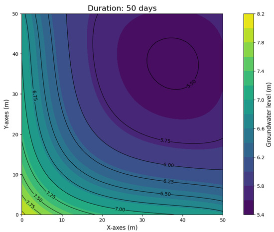
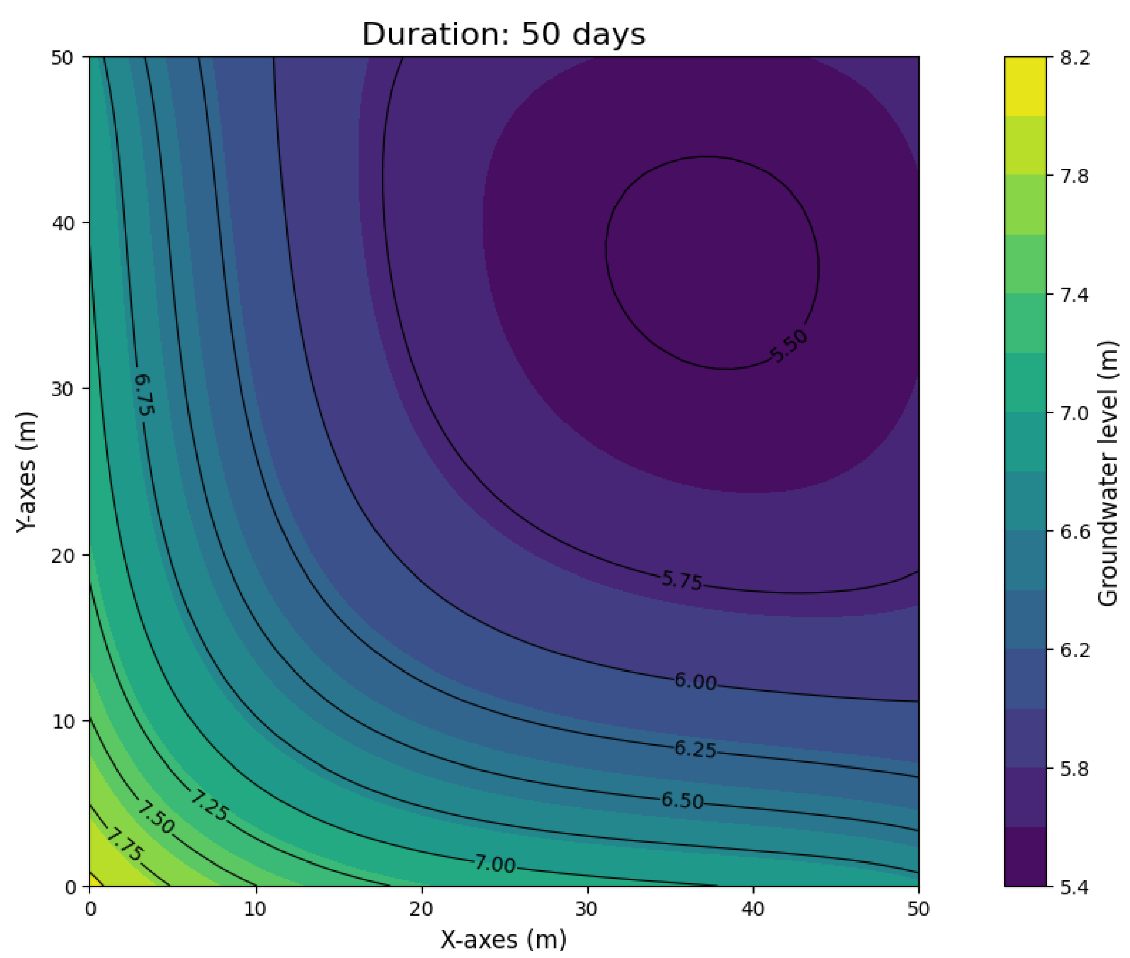
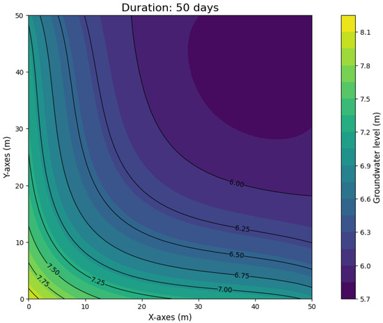
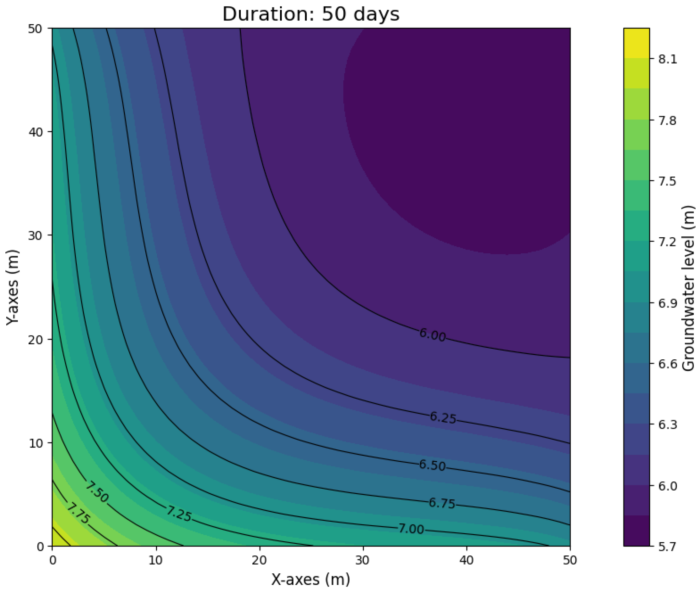
Figure 2 shows the “pessimistic” prediction of the linear model after 50 days of drought. According to it, in the northeastern part of the field, the water level will drop to 5.5 m, which is significantly lower than the established agronomic threshold of 6.0 m.

Figure 2. Changes in groundwater level based on the law of linear evaporation.

In contrast, according to the results of the nonlinear model shown in Figure 3, the water level in the same area stabilizes around 6.0 m. This phenomenon demonstrates the self-regulation mechanism of the nonlinear model: as the water level approaches the critical point, the evaporation intensity decreases sharply, which prevents further decrease in the water level.

Figure 3. Changes in groundwater level based on the law of nonlinear evaporation.

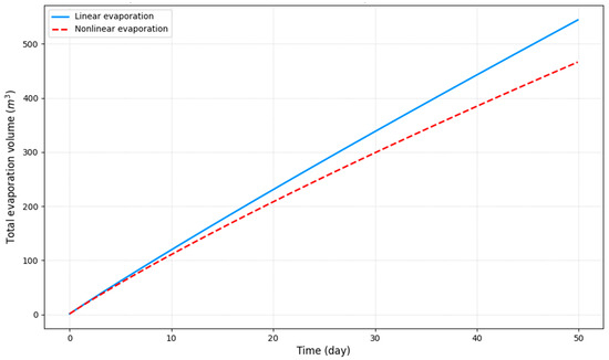
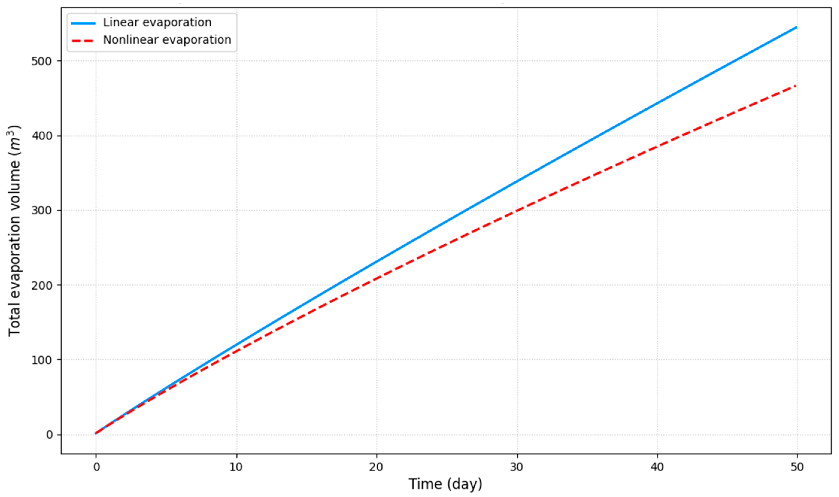
The main reason for the difference between these two results is shown in Figure 4. The linear model (continuous line) continues to evaporate water at an almost constant intensity over time. The nonlinear model (dotted line) reduces the rate of evaporation (the slope of the curve) as the water level decreases, reflecting the system’s water “saving” characteristic.

Figure 4. Comparison of linear and nonlinear evaporation volumes over time.

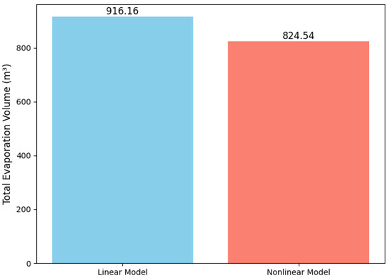
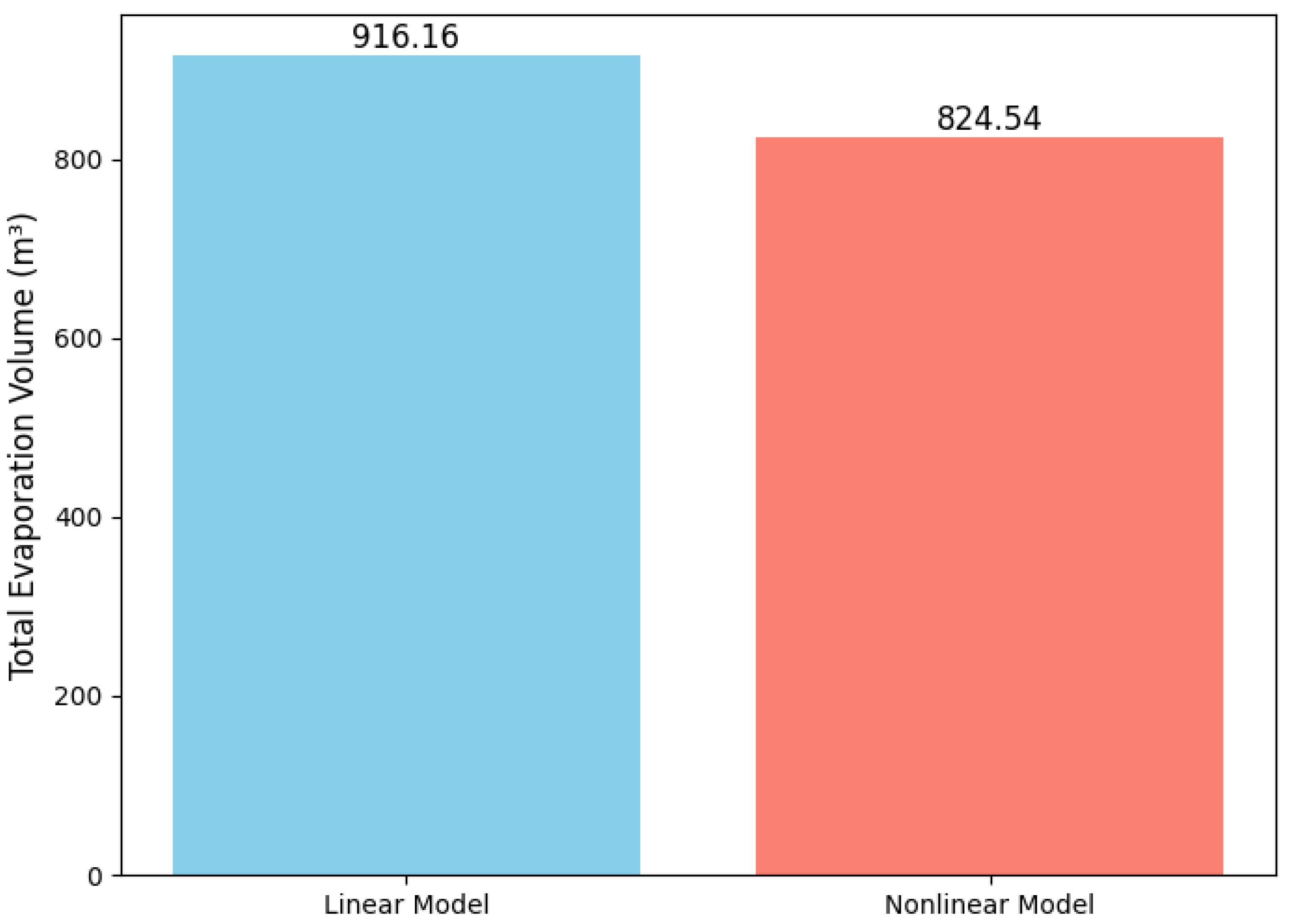
The quantitative difference in total water losses is clearly illustrated in Figure 5. Under scenario 2, at the end of 50 days, the linear model predicted 91.6 m3 (or ~11%) more water evaporation than the nonlinear model (916.16 m3 versus 824.54 m3). Sensitivity analysis showed that under even more severe conditions, such as scenario 3 (“Extreme Drought”), this difference could exceed 30%.

Figure 5. Total Evaporation Volume over 50 Days.

4.3. Validating the Model with Field Data

To validate the theoretical advantages of the proposed nonlinear model in practice and evaluate its accuracy in describing real hydrogeological processes, it was tested against field data. This section presents the data used for validation, the methodology applied, and an analysis of the obtained results.

4.3.1. Model Parameterization and Determination of Main Hydrogeological Indicators

To maximize the model’s alignment with the real conditions of the experimental site in the Zarafshan River valley and ensure the reliability of validation results, the main hydrogeological parameters were determined using a comprehensive set of field and laboratory studies.

Transmissivity coefficient (T): The transmissivity coefficient (T) of the main aquifer was determined using pumping tests conducted at the KZ-1 observation well, located at the center of the experimental site. The pumping test lasted 72 h, with groundwater level drawdown continuously measured in three observation piezometers located 10, 25, and 50 m from the central well. The obtained data were analyzed using Theis’s non-steady flow formula [24]. Calculations revealed that the average hydraulic conductivity value for the main aquifer is T = 180 m²/day. This value falls within the range typical for alluvial deposits.

Filtration coefficient (k_g): The filtration coefficient of the upper confining layer (k_g) was determined under laboratory conditions. For this purpose, undisturbed soil samples were taken from the confining layer at depths of 1.5 m, 3.0 m, and 4.5 m during piezometer drilling. In the laboratory, these samples were tested using a constant-head permeameter. Analysis results showed that the average filtration coefficient of the layer is k_g = 0.8 m/day.

Specific yield coefficient (μ_v): The specific yield coefficient (μ_v) for the upper confining layer was also calculated based on laboratory analyses. The aforementioned soil samples were first fully saturated with water, and then the volume of water freely draining under the influence of gravity was measured. The results were expressed as a percentage of the total soil volume. The experiment revealed that the soil texture is sandy loam, and its specific yield coefficient is μ_v = 0.18. This value corresponds to those reported in scientific literature for sandy loam soils.

The parameters obtained through these field and laboratory studies were incorporated into the model, establishing a foundation for verifying the correspondence of its forecast results with actual field data.

4.3.2. Research Area and Field Data

For validation, an experimental plot measuring 50 × 50 m in the Zarafshan River valley was selected. Daily fluctuations in groundwater levels were measured at the KZ-1 observation well located in this area during a 50-day dry period from 1 June to 20 July 2024. During this period, almost no precipitation was observed, which allowed for a clear study of the evaporation process’s influence on the groundwater regime. Daily data (air temperature, potential evapotranspiration) from the Zarafshan agrometeorological station, located 3.2 km from the study area, were used as input parameters for the model. This distance is considered acceptable for ensuring uniform microclimatic conditions.

4.3.3. Validation Methodology

During the validation process, model calculations were carried out for both cases of the Krylov–Averyanov law—linear (n = 1) and nonlinear (n = 2). The actual groundwater level measured at the KZ-1 well on June 1 was input into the model as an initial condition.

To quantitatively assess the degree of correspondence between the models and the observed data, the following statistical indicators were used:

• Root Mean Square Error (RMSE): This indicates the average deviation of the model results from the actual values. The closer its value is to zero, the more accurate the model is considered to be.

$$RMSE=\sqrt{\frac{{\displaystyle \sum _{i=1}^N{(h_{sim,i}-h_{obs,i})}^2}}{N}}$$

where $h_{sim}$—modeled level; $h_{obs}$—observed level; N—number of observations.

2.

Nash-Sutcliffe Efficiency (NSE): This evaluates the model’s predictive capability. The closer its value is to 1, the more reliable the model. If $NSE\le 0$, it indicates that the model results are worse than the average value of the observations.

$$NSE=1-{\displaystyle \frac{{\displaystyle \sum _{i=1}^N{(h_{sim,i}-h_{obs,i})}^2}}{{\displaystyle \sum _{i=1}^N{(h_{sim,i}-{\overline{h}}_{obs,i})}^2}}}$$

where ${\overline{h}}_{obs}$ is the average value of the observed levels.

4.3.4. Results and Analysis

The calculation results of both models for a 50-day period were compared with actual observations from the KZ-1 well.

As evident from the table, the RMSE value of the nonlinear model (0.09 m) is more than three times lower than that of the linear model (0.28 m), indicating its significantly higher accuracy (Table 2). Furthermore, the NSE value calculated for the nonlinear model, which equals 0.94 (very close to 1), confirms that its predictive ability is “very high.” In contrast, the NSE value of 0.65 for the linear model can only be assessed as “satisfactory.”

Table 2. Statistical accuracy indicators of the models.

Model Type	RMSE (m)	NSE
Linear model (n = 1)	0.28	0.65
Nonlinear model (n = 2)	0.09	0.94

5. Conclusions

The conducted analysis and experiments demonstrate that when the groundwater level fluctuates around the critical depth affecting evaporation, the use of a simple linear model leads to an artificial overestimation of water losses. The nonlinear model more accurately reflects intensive evaporation at high water levels and its sharp decrease as the level drops, which corresponds to real physical processes, such as the reduced efficiency of capillary rise.

The difference of ~11% in the model results may seem insignificant for a small area, but it should be noted that this error is systematic. If this approach were applied to a larger area, for example, 5 × 5 km, the volume of water lost could amount to millions of cubic meters. This indicates that selecting the correct evaporation model for long-term water resource planning is of great economic importance.

In conclusion, to reliably predict the groundwater regime under conditions of water scarcity and climate change, it is crucial to model physically based nonlinear processes that more closely reflect real-world conditions.

In this study, validation is limited to data from a single well. In the future, using data from multiple wells to verify that the model accurately reflects spatial distribution will further enhance the model’s reliability.

References

- State of Global Water Resources 2023 Report. World Meteorological Organization, WMO-No.1362. 2024. Available online: https://wmo.int/zh-hans/news/media-centre/wmobaogaoqiangdiaoquanqiushuiziyuanriyiduanquehejinzhang (accessed on 7 October 2024).
- Condon, L.E.; Kollet, S.; Bierkens, M.F.P.; Fogg, G.E.; Maxwell, R.M.; Hill, M.C.; Fransen, H.H.; Verhoef, A.; Van Loon, A.F.; Sulis, M.; et al. Global Groundwater Modeling and Monitoring: Opportunities and Challenges. Water Resour. Res. 2021, 57, e2020WR029500. [Google Scholar] [CrossRef] [Scilit]
- Sutanudjaja, E.H.; van Beek, L.P.H.; Wanders, N.; Wada, Y.; Bosmans, J.H.C.; Drost, N.; van der Ent, R.J.; de Graaf, I.E.M.; Hoch, J.M.; de Jong, K.; et al. PCR-GLOBWB 2: A 5 arcmin global hydrological and water resources model. Geosci. Model Dev. 2018, 11, 2429–2453. [Google Scholar] [CrossRef] [Scilit]
- Amini, M.; Rasoulzadeh, A.; Azizi Mobaser, J.; Hamdi Ahmadabad, Y.; Pollacco, J.A.P.; Fernández-Gálvez, J. Hydro-pedotransfer functions to estimate evaporation from bare soil surface in semi-arid regions. Environ. Res. Commun. 2025, 7, 11786221251349047. [Google Scholar] [CrossRef] [Scilit]
- de Graaf, I.E.M.; Gleeson, T.; van Beek, L.P.H.; Sutanudjaja, E.H.; Bierkens, M.F.P. A global-scale two-layer transient groundwater model: Development and application to groundwater depletion. Adv. Water Resour. 2017, 102, 53–67. [Google Scholar] [CrossRef] [Scilit]
- Bakker, M. The effective vertical anisotropy of layered aquifers. Groundwater 2025, 63, 45–58. [Google Scholar] [CrossRef] [Scilit]
- Bear, J. Dynamics of Fluids in Porous Media; American Elsevier Publishing Company: New York, NY, USA, 1972; 764p. [Google Scholar]
- Hantush, M.S. Modification of the theory of leaky aquifers. J. Geophys. Res. 1960, 65, 3713–3725. [Google Scholar] [CrossRef] [Scilit]
- Lei, K.; Ma, F.; Liu, J.; Luo, Y.; Cui, W.; Zhou, Y.; Liu, H.; Wang, X.; Tian, M.; Zhao, L. Leaking Recharge Mechanism in the Multi-Layer Aquifer System of a Typical Land Subsidence Area in Beijing. Proc. IAHS 2020, 382, 309–314. [Google Scholar] [CrossRef] [Scilit]
- Shah, N.; Nachabe, M.; Ross, M. Extinction depth and evapotranspiration from ground water under selected land covers. Ground Water 2007, 45, 329–338. [Google Scholar] [CrossRef] [Scilit]
- Scanlon, B.R.; Fakhreddine, S.; Rateb, A.; de Graaf, I.; Famiglietti, J.; Gleeson, T.; Grafton, R.Q.; Jobbagy, E.; Kebede, S.; Kolusu, S.R.; et al. Global water resources and the role of groundwater in a resilient water future. Nat. Rev. Earth Environ. 2023, 4, 87–101. [Google Scholar] [CrossRef] [Scilit]
- Sophocleous, M. Interactions between groundwater and surface water: The state of the science. Hydrogeol. J. 2002, 10, 52–67. [Google Scholar] [CrossRef] [Scilit]
- Doble, R.C.; Crosbie, R.S. Review: Current and emerging methods for catchment-scale modelling of recharge and evapotranspiration from shallow groundwater. Hydrogeol. J. 2017, 25, 3–23. [Google Scholar] [CrossRef] [Scilit]
- Averyanov, S.F. Filtration from Canals and Its Influence on Groundwater Regime; Kolos: Moscow, Russia, 1982; p. 237. [Google Scholar]
- Wang, H.F.; Anderson, M.P. Introduction to Groundwater Modeling: Finite Difference and Finite Element Methods; W.H. Freeman and Company: San Francisco, CA, USA, 1982; 237p. [Google Scholar]
- Langevin, C.D.; Hughes, J.D.; Banta, E.R.; Provost, A.M.; Niswonger, R.G.; Panday, S. Documentation for the MODFLOW 6 Groundwater Flow Model—Version 6.3.0; U.S. Geological Survey Techniques and Methods, Book 6, Chapter A55; U.S. Geological Survey: Reston, VA, USA, 2022; 215p. [Google Scholar]
- Kuffour, B.N.O.; Engdahl, N.B.; Woodward, C.S.; Condon, L.E.; Kollet, S.; Maxwell, R.M. ParFlow v3.5.0 Documentation: Integrated Hydrologic Model; Technical Report LLNL-SM-813485; Lawrence Livermore National Laboratory: Livermore, CA, USA, 2020. [Google Scholar]
- Daliev, S.; Ravshanov, N. Numerical and mathematical modeling of changes in groundwater levels in two-layer media. In Proceedings of the 2022 International Conference on Information Science and Communications Technologies (ICISCT), Tashkent, Uzbekistan, 28–30 September 2022. [Google Scholar]
- Ravshanov, N.; Daliev, S. Non-linear mathematical model to predict the changes in underground water level and salt concentration. J. Phys. Conf. Ser. 2020, 1441, 012163. [Google Scholar] [CrossRef] [Scilit]
- Mansour, M.; Walthall, S.; Hughes, A. The Importance of Using Multi-Level Piezometers to Improve the Estimation of Aquifer Properties from Pumping Tests in Complex Heterogeneous Aquifers. Water 2025, 17, 2338. [Google Scholar] [CrossRef] [Scilit]
- Zlotnik, V.A.; Cardenas, M.B.; Toundykov, D. Effects of multiscale anisotropy on basin and hyporheic groundwater flow. Ground Water 2011, 49, 576–583. [Google Scholar] [CrossRef] [Scilit]
- Janssen, J.; Tootchi, A.; Ameli, A.A. Tackling Water Table Depth Modeling via Machine Learning: From Proxy Observations to Verifiability. Adv. Water Resour. 2025, 201, 104955. [Google Scholar] [CrossRef] [Scilit]
- Hung, W.C.; Hwang, C.; Chang, C.P.; Yen, J.Y.; Liu, C.H.; Yang, W.H. Modeling compaction of multi-layer aquifer system due to groundwater withdrawal. Eng. Geol. 2015, 187, 143–155. [Google Scholar]
- Zipper, S.C.; Dallemagne, T.; Gleeson, T.; Boerman, T.C.; Hartmann, A. Groundwater pumping impacts on real stream networks: Testing the performance of simple management tools. Water Resour. Res. 2023, 54, e2022WR032134. [Google Scholar] [CrossRef] [Scilit]
- Camporese, M.; Paniconi, C.; Putti, M.; Orlandini, S. Surface–Subsurface Flow Modeling with Path-Based Runoff Routing, Boundary Condition-Based Coupling, and Assimilation of Multisource Observation Data. Water Resour. Res. 2010, 46, W02512. [Google Scholar] [CrossRef] [Scilit]
- Rubin, J. Theoretical analysis of two-dimensional, transient flow of water in unsaturated and partly unsaturated soils. Soil Sci. Soc. Am. J. 1968, 32, 607–615. [Google Scholar] [CrossRef] [Scilit]
- Zhang, Q.; Volker, R.E.; Lockington, D.A. Experimental Investigation of Contaminant Transport in Coastal Groundwater. Adv. Environ. Res. 2002, 6, 229–237. [Google Scholar] [CrossRef] [Scilit]
- Feng, F.; Ghorbani, H.; Radwan, A.E. Predicting groundwater level using traditional and deep machine learning algorithms. Front. Environ. Sci. 2024, 12, 1291327. [Google Scholar] [CrossRef] [Scilit]
- Igwebuike, N.; Ajayi, M.; Okolie, C.; Kanyerere, T.; Halihan, T. Application of Machine Learning and Deep Learning for Predicting Groundwater Levels in the West Coast Aquifer System, South Africa. Earth Sci. Inform. 2025, 18, 6. [Google Scholar] [CrossRef] [Scilit]
- Vahdat-Aboueshagh, H.; Tsai, F.T.C. Irrigation-intensive groundwater modeling of complex aquifer systems through integration of big geological data. Front. Water 2021, 3, 623476. [Google Scholar] [CrossRef] [Scilit]
- Batelaan, O.; De Smedt, F. GIS-based recharge estimation by coupling surface–subsurface water balances. J. Hydrol. 2007, 337, 337–355. [Google Scholar] [CrossRef] [Scilit]
- Condon, L.E.; Maxwell, R.M. Simulating the sensitivity of evapotranspiration and streamflow to large-scale groundwater depletion. Sci. Adv. 2019, 5, eaav4574. [Google Scholar] [CrossRef] [Scilit]
- Sahoo, S.; Russo, T.A.; Elliott, J.; Foster, I. Machine learning algorithms for modeling groundwater level changes in agricultural regions of the U.S. Water Resour. Res. 2017, 53, 3878–3895. [Google Scholar]
- Wunsch, A.; Liesch, T.; Broda, S. Groundwater level forecasting with artificial neural networks: A comparison of long short-term memory, convolutional neural networks, and non-linear autoregressive networks with exogenous input. Hydrol. Earth Syst. Sci. 2021, 25, 1671–1687. [Google Scholar] [CrossRef] [Scilit]
- Zeng, X.; Decker, M. Improving the numerical solution of soil moisture-based Richards equation for land models with a deep or shallow water table. J. Hydrometeorol. 2009, 10, 308–319. [Google Scholar] [CrossRef] [Scilit]
- Brunner, P.; Simmons, C.T. HydroGeoSphere: A fully integrated, physically based hydrological model. Ground Water 2012, 50, 170–176. [Google Scholar] [CrossRef] [Scilit]
- Paniconi, C.; Putti, M. Physically Based Modeling in Catchment Hydrology at 50: Survey and Outlook. Water Resour. Res. 2015, 51, 7090–7129. [Google Scholar] [CrossRef] [Scilit]
- Brunner, P.; Therrien, R.; Renard, P.; Simmons, C.T.; Franssen, H.J.H. Advances in understanding river–groundwater interactions. Rev. Geophys. 2017, 55, 818–854. [Google Scholar] [CrossRef] [Scilit]
- Fleckenstein, J.H.; Krause, S.; Hannah, D.M.; Boano, F. Groundwater–surface water interactions: New methods and models to improve understanding of processes and dynamics. Adv. Water Resour. 2010, 33, 1291–1295. [Google Scholar] [CrossRef] [Scilit]
- Dagan, G.; Neuman, S.P. Subsurface Flow and Transport: A Stochastic Approach; Cambridge University Press: Cambridge, UK, 1997; p. 241. [Google Scholar]
- Peaceman, D.W.; Rachford, H.H. The numerical solution of parabolic and elliptic differential equations. J. Soc. Ind. Appl. Math. 1955, 3, 28–41. [Google Scholar] [CrossRef] [Scilit]
- An, H.; Ichikawa, Y.; Tachikawa, Y.; Shiiba, M. A New Iterative Alternating Direction Implicit (IADI) Algorithm for Multi-Dimensional Saturated–Unsaturated Flow. J. Hydrol. 2011, 408, 127–139. [Google Scholar] [CrossRef] [Scilit]
- Bellman, R.E.; Kalaba, R.E. Quasilinearization and Nonlinear Boundary-Value Problems; Elsevier: New York, NY, USA, 1965. [Google Scholar]
- Mukhamadiyev, A.; Karimov, M. Model of Aquifer-Level Changes Based on Evaporation Intensity and Infiltration Coefficient. Mathematics 2025, 13, 2562. [Google Scholar] [CrossRef] [Scilit]
Disclaimer/Publisher’s Note: The statements, opinions and data contained in all publications are solely those of the individual author(s) and contributor(s) and not of MDPI and/or the editor(s). MDPI and/or the editor(s) disclaim responsibility for any injury to people or property resulting from any ideas, methods, instructions or products referred to in the content. |
© 2026 by the authors. Licensee MDPI, Basel, Switzerland. This article is an open access article distributed under the terms and conditions of the Creative Commons Attribution (CC BY) license.