


Abstract
The article discusses the control of nonlinear processes with first-order dominant dynamics, focusing on implementation using modern hardware available in various programmable devices and embedded systems. The first two approaches rely on linearization with an ultra-local process model, considering small changes of the process input and output around a fixed operating point, which can be adjusted through gain scheduling with the setpoint variable. This model is used to configure either the historically established automatic reset controller (ARC) or a stabilizing proportional (P) controller enhanced by an inversion-based disturbance observer (DOB). This solution can be interpreted as an application of modern control theory (MCT), as DOB-based control (DOBC) or as advanced disturbance rejection control (ADRC). Alternatively, they can be viewed as a special case of automatic offset control (AOC) based on two types of linear process models. In the third design method, setpoint tracking by exact linearization (EL) is extended with a nonlinear DOB designed using the inverse of the nonlinear process dynamics (EEL). The fourth approach augments EL-based tracking with a DOB derived from the transfer functions of nonlinear processes (NTF). An illustrative example involving the control of a liquid reservoir with a variable cross-section clarifies motivation for the definition of (linear) local and ultra-local process models as well as their advantages in designing robust control that accounts for process uncertainties. Thus, the speed, homogeneity, and shape of transient responses, the ability to reconstruct disturbances, control signal saturation, and measurement noise attenuation are evaluated according to the assumptions specified in the controller design. The novelty of the paper lies in presenting a unifying perspective on several seemingly different control options under the impact of measurement noise. By explaining their essence, advantages, and disadvantages, it provides a foundation for controlling more complex time-delayed systems. The paper emphasizes that certain aspects of controller design, often overlooked in traditional linearization procedures, can significantly improve closed-loop properties.
Keywords:
automatic reset; automatic offset; disturbance observer; ADRC; nonlinear control; linearization; gain scheduling; exact linearization; nonlinear transfer functions; constrained control MSC:
93B52
1. Introduction
Discovered in 1930s, automatic reset controllers (ARCs) have been among the most widely used solutions in automatic control for decades. Despite the abundance of instructions for their correct use, their essence has never received attention corresponding to their significance. Interesting details of ARC development are given, for example, in [1]. However, their original designation has fallen into disuse and has been replaced by the only partially accurate acronym PID ( from proportional–integral–derivative) controllers. Drawing attention to this terminological problem is not just a matter of taste. The incorrect designation and resulting misinterpretation of PID controllers are, in fact, obstacles to their understanding and further development [2]. PID controllers limit the study of ARCs to the proportional control band, which, without sufficient consideration, led to problems such as integrator windup. Windup can be eliminated [3,4,5,6,7,8,9,10], but it complicates controller design. For a long time, PID controllers also overshadowed the search for connections between ARCs and other contemporary approaches and structures in automatic control. Thus, given the prominent position of the ARC in automatic control, this article begins with issues surrounding its use and generalization in a nonlinear context based on disturbance observer-based control (DOBC). The term disturbance observer (DOB) was first used in automatic control theory in the second half of the 1980s [11,12,13,14,15]. It appeared in connection with the development of structures for disturbance compensation, which were intended to improve upon the results achieved with PID controllers. However, the pioneers of DOBC did not notice the key fact that the basics of DOB can be found even in PID controllers themselves, more precisely in the most frequently used industrial controllers originally called automatic reset [1,2,16,17]. ARC has only recently been explained as a model-based approach with a simplified DOB designed on the basis of integrative first-order models with a simplified structure [18]. This neglected both integrator inversion and possible process dead time. These DOB simplifications reflected the limited capabilities of the original analog (pneumatic) implementations [18]. The dead time of the process model was implicitly considered by one of the first controller tuning methods, which approximated the step response by a tangent through the inflection point [19]. However, in ARCs, dead time was used only for controller tuning. One of the most important advantages of modern programmable control devices is increased processing power, which makes it possible to use full-scale DOBs that include inversion of the process model together with the process dead-time model. The full-scale DOB allows for separate design of the stabilizing controller and the DOB itself. In the nominal case, the DOB does not affect the dynamics of the stabilization processes [17]. This is analogous to the separate treatment of stabilization and state reconstruction that appeared in state-space-based approaches of modern control theory (MCT) [20,21,22,23]. However, although MCT rigorously solved numerous problems in automatic controller design, it failed to address two serious issues. First, by misunderstanding the previous phase of development, it started from distorted interpretations of industrial ARCs as PID controllers and did not develop them further in a correct manner. Moreover, MCT emerged during the dominance of analog technology, when controllers designed in the continuous-time domain did not include dead-time elements. These appeared only in postmodern internal model control (IMC) structures [24], developed from the Smith predictor [25] with reconstruction and compensation of output disturbances by a parallel process model. In IMC, reconstruction of output disturbances resulted in correction of the setpoint values of the remaining loop, equivalent to feedforward control. However, this concept could not be used without modifications to control unstable and marginally stable processes. For integrating systems, the output disturbance can be shown to be unobservable [26]. Even unstable open-loop processes cannot be addressed in the feedforward control concept.
Understanding ARC as a model-based structure with a stabilizing controller and a simplified DOB designed for single integrator plus dead-time (IPDT) process models has recently enabled [18] their generalization to controllers using higher-order (HO) derivatives [18,27]. HO derivatives have been shown to reduce the impact of dead time through “approximate inversion.” By improving disturbance response, this also allows the replacement of more complex local linear models with simplified ultra-local (integral) models [28]. The effort to generalize ARC to HO process models ultimately led to the concept of automatic offset controllers (AOCs) [29]. However, in this article, the AOC concept will be presented only in a simplified context for systems with dominant first-order dynamics. The closed-loop dead time, which is important for adding missing process information when using ultra-local models (compared to local models), will be addressed only briefly. It will be necessary to make assumptions about achieving equivalent performance when using both local and ultra-local models.
Definition 1
(AOC for processes with a dominant first-order dynamics). For a generally nonlinear process with dominant first-order dynamics, the AOC consists of a stabilizing P controller possibly supplemented by an “approximate inversion” of the loop dead time using the feedback controller with mth-order derivatives. The stabilizing control is augmented by a DOB including the model dead time. The DOB inverts the process model to reconstruct and compensate for external and internal disturbances.
The concept of AOC, formulated with the distinction between two types of linear models, addresses the long-standing neglect of the linearization problem in the control of nonlinear processes [17] and time-delayed systems. In the simulations presented in this paper for evaluating different controllers, loop dead-time and its possible compensation are neglected, corresponding to . Both the P and DOB designs can be based on local or ultra-local process models, which correspond to process linearization around a chosen equilibrium point. The use of ultra-local models is motivated by controller simplification and robust control aspects. AOC, incorporating ultra-local models, helps to demonstrate mutual connections among ARC, MCT, DOB-based control (DOBC) [11,12,15,30], and other widely used automatic control methods, such as active disturbance rejection control (ADRC) [31,32,33,34,35,36,37,38,39]. Another control approach, developed within flatness-based control [40] and known as intelligent PID control, is also referred to as model-free control [41]. Understanding the similarities and significant differences among these alternatives should contribute to a more effective deployment and improved teaching of control for simple nonlinear processes. Highlighting and confronting the key features of the alternative approaches considered is the most effective way to reduce the ever-growing amount of knowledge. Thus, this can help keep the overall expanding content of the automatic control discipline to be sustainably understandable. Linearization of nonlinear processes to obtain a linear model that simplifies controller calculation has been present since the early periods of control (see, e.g., [42]). Numerous textbooks are available on nonlinear systems [43,44,45], as well as on differential geometric [46] and algebraic methods [47]. The latter have been generalized by introducing transfer functions to nonlinear systems [48]. There has also been significant development of methods that extend linear techniques to nonlinear processes, such as gain scheduling [43,49,50,51,52,53,54,55,56]. The large number of professional journals and conferences focused on nonlinear control suggests continued interest in this area of automatic control. However, there are also completely opposite indications, as shown, for example, by the IFAC survey [57], which reveals a widespread lack of awareness of the progress achieved. This does not indicate a health of research environment in the nonlinear control area, but may point to a problem of misunderstanding the essence that all other postmodern approaches have adopted since the emergence of MCT in the 1960s. We will demonstrate this with three common shortcomings: The design of control for nonlinear systems is often implemented by linearizing them, considering small increments of input and output around a chosen equilibrium point. However, it is not always verified whether such work with small increments is actually imposed on the system by the control structure itself. Paper [17] recently demonstrated that the ARC structure can inherently support linearization for small input and output changes around a fixed operating point when extended with appropriate gain scheduling and signal injections to ensure small deviations from equilibrium. Therefore, its use in programmable devices can be successfully extended to the control of nonlinear processes without significant modifications. Omitting these injections is possible but will generate fictitious disturbances and cause some deterioration in control performance. When linearizing the process by introducing small increments in input and output, another important consideration arises. Traditional approaches have mostly sought to fully utilize the available partial derivatives. However, this can be unnecessarily complex or even unfeasible, and it does not always yield better control results. The second important aspect of linearization examined in the article is therefore the use of two types of linear process models.
The third overlooked point regarding the linearization of nonlinear processes emerged with the development of control technology. Implementing gain scheduling using programmable devices and embedded systems does not require the traditional ARC design with a simplified DOB. By omitting DOB simplification, at least nominally, loop stabilization and disturbance compensation can be considered separately. However, since the linearized model generally only approximates a nonlinear process, after changes in the scheduling parameter—even when no external disturbance affects the system—the linearization-based DOB registers a nonzero disturbance. In situations requiring advanced reconstruction and disturbance compensation, there may be motivation to use more advanced DOBs that are not limited to small deviations from the operating point. If, in this paper, we illustrate a nonlinear system with dominant first-order dynamics, such as a liquid reservoir, many of the resulting observations may also apply to other current engineering problems through physical analogies. This may include the accumulation of kinetic energy and the elimination of external disturbances in vehicle systems [58]. Alternatively, precise reconstruction of disturbances may be required in the control and monitoring of fuel cells, which are increasingly used as energy storage devices (see, e.g., [59,60]).
Since the discovery of ARC, many alternatives have emerged. Exact linearization (EL), developed within the framework of differential geometry [46] and also known as feedback linearization, arose from the idea of eliminating nonlinear process feedback by applying a counteracting signal. This allows the controller to use linear feedback. An important similarity between the ARC design and the EL controller is that stabilization in EL is also designed for a pure integrator system. However, while the ARC design reduces the nonlinear feedback of the process to an approximation by a constant, the EL design transforms the initial nonlinear system into a pure integrator by introducing counteracting feedback, thereby eliminating the internal process nonlinearity. To compensate for possible external or internal disturbances, an extension of the EL controller, denoted as EEL, will be proposed. It uses a nonlinear DOB based on the differential equation of the first-order process.
Another alternative for the analysis and synthesis of nonlinear processes was developed using algebraic methods, resulting in the generalization of the transfer function methodology, which was previously used only in linear systems. Thus, a nonlinear DOB can also be designed for EL using the nonlinear transfer function (NTF) methodology.
To provide a practical demonstration of the unifying saturated design for first-order nonlinear processes using ARC, AOC, EEL, and NTF, the remainder of this paper is organized as follows. Section 2 presents the gain-scheduled model-based controller design, which utilizes a full disturbance observer (DOB) including the inverse ultra-local process model (denoted as DOBC). This approach generalizes the simplified DOB of ARCs by incorporating process model inversion, which is neglected in the simplified version. Both ARC and AOC are applied to an illustrative example of a nonlinear liquid tank with a variable cross-section, as considered in [17]. The discussion of possible process uncertainties explains the critical aspects of local model identification and highlights the advantages of the simpler ultra-local model. It also shows how the reduced precision of ultra-local models can be offset by decreasing loop dead time and storing information obtained from previous transient response evaluations. Section 3 introduces two additional alternatives, EEL and NTF. Both linear and saturating controllers were tested by simulation, both without measurement noise and with noise introduced as random numbers. The resulting transients are evaluated by quantifying them with modified monotonicity-based performance measures. This assesses deviations of the process output and input from ideal transients, considering a specified number of monotonic segments in the controller design. The paper concludes with a summary of the main findings and novel contributions in the Section 5.
2. Linearization-Based Constrained Controller Design
The structure of automatic reset-based controllers can be derived from the need to control integrative (ultra-local) first-order processes. However, its use can be extended both to the control of time-delayed processes [18] and to the control of much more complex nonlinear processes with dominant dynamics described for by a differential Equation [17]
Here, represents the output of the process, is its input, and f is a function differentiable with respect to both variables y and u. Using the Taylor series expansion,
around an operating point specified as
and considering just small increments of the input and output
the system can be approximated by linear model
For sufficiently small deviations (4) from X,
the system (1) can be characterized by a Laplace transfer function
Hence, the operating point symbol X can be omitted for the sake of simplicity. Several model-based approaches have been discussed, for example, in [26]. Those based on ultra-local models, in which is formally considered, are particularly suitable for application due to their simplicity. This means that obtaining the term that requires partial derivatives of f with respect to y can simply be omitted [17]. This procedure is typically used, but not consistently enough, in ADRC.
2.1. Input Disturbance Reconstruction and Compensation
Several possible approaches to reconstruction of an input disturbance have been formulated for the first-order system (1) with an ultra-local model corresponding to . The difference between the actual input to the process model in (7) and the controller output can be represented as the reconstructed input disturbance
In disturbance observer-based control (DOBC), the input of the model can be simply calculated from its output by means of transfer functions according to
To compensate for the dynamics of the filter used to calculate in (8)–(9), the same filter must also be applied to the output of the controller . This provides a filtered reconstructed disturbance
This formula can be written as follows:
Its use can be encountered in several model-based approaches.
Remark 1
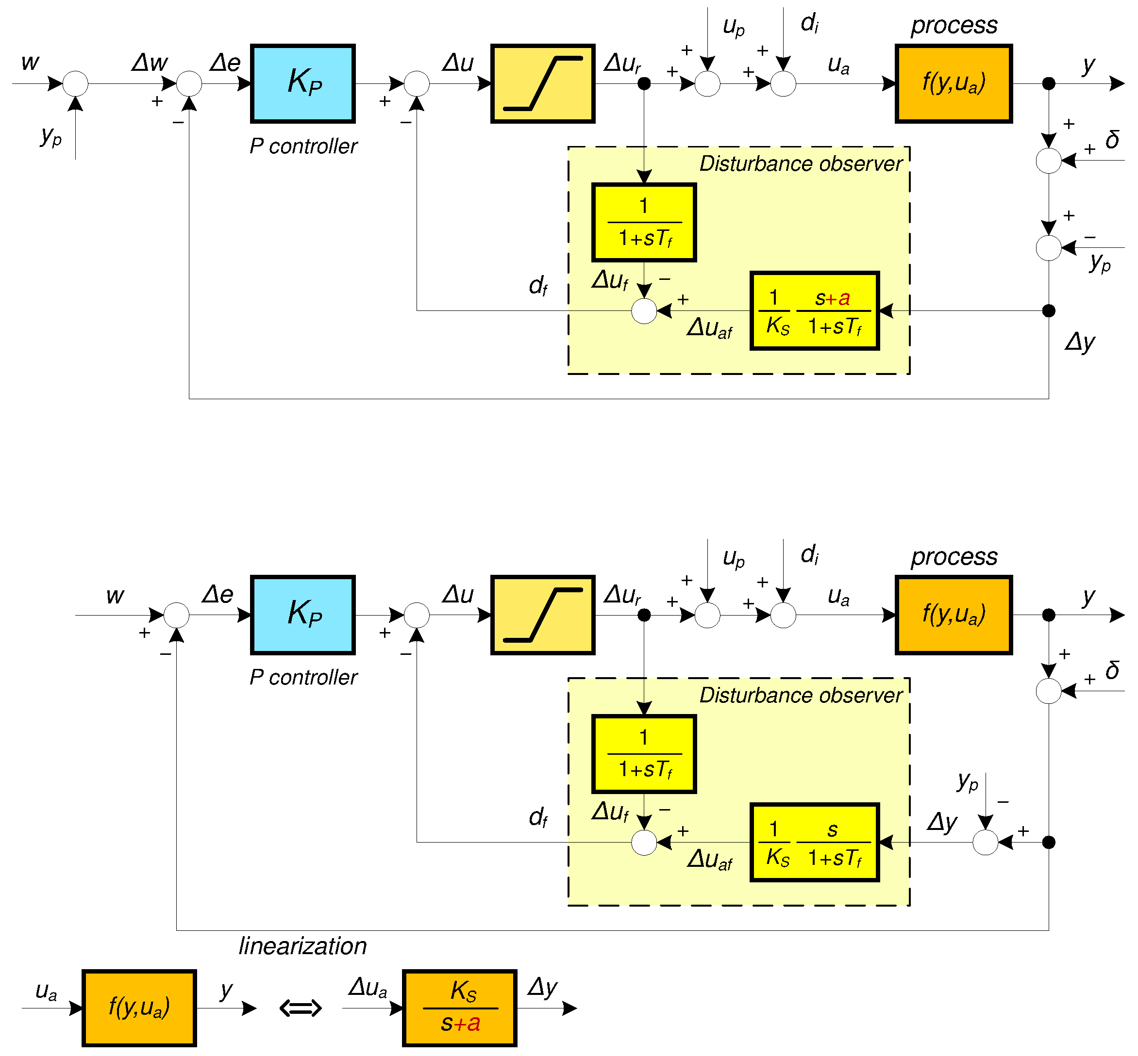
(ARC, MCT, DOBC, ADRC and AOC). Based on the linearization of the process (7), the DOB-based controller (DOBC) can be created using a polynomial formulation of the reconstructed input disturbance as the difference between the reconstructed input to the process model and the output of the controller (11) [11,12,15,30,61,62]. For inversion of the dominant first-order model, a filter with is usually used. However, in DOBC, it would formally be possible to use all integer values . Figure 1 above shows a possible implementation of a whole family of linearization-based control systems of (1) with the setpoint w.
ADRC [31,63,64,65,66,67,68,69,70] uses for the derivation of the DOB the state-space approaches of MCT [20,21,22,23,71]. The disturbance reconstruction is implemented by an extended state observer (ESO) representing mostly an identical Luenberger observer designed for “ultra-local” (integral) process model with (ULM) in (7) and in (11). The derivation of a reduced ESO that would allow (11) with is considerably rarer.
The modeling errors resulting from the use of ULM with are usually merged with external disturbances into “a lumped or total disturbance”. However, in MCT, ESO was used for a long time before pioneering work in ADRC [31,63] and was not limited to working with ultra-local models considering and . Leaving aside the historical context and details of the usual setup and interpretation, ADRC and DOBC can be considered equivalent approaches. In the context of compensating for nonlinear process properties with injection of operating points and possible transport delay, we will interpret all DOB-based controllers using (11) as special cases of automatic offset control (AOC).
In ARC, the overall DOB design is further simplified by choosing with in (11). Despite this simplification, it is still useful to consider ARC as a special case of model-based control.
Figure 1.
Proportional controller with a DOB derived by linearization of nonlinear processes (1) using local and ultra-local models based on small increments around the operating point ) (3), with subtracted from the process output y and added as the controller offset to (above); the alternative scheme with shifted summation points, formulated just for ultra-local model (neglecting the red term ) (middle); -measurement noise and equivalence of the nonlinear process and its linearization for small input and output increments (below).
2.2. Dynamics of Nominal ARC and AOC
For the “nominal” ultra-local model and the stabilizing controller gain , the closed-loop characteristic polynomial is
A stable closed-loop pole can be replaced with a positive closed-loop time constant
The gain can thus be expressed in terms of as
The differences between ARC and AOC (including DOBC and ADRC) occur for activated reconstruction and compensation of disturbances. When using the full DOB of AOC with in the nominal case with zero external disturbance , the reconstructed disturbance will also be zero, . Therefore, the full nominal DOB does not affect the dynamics of the setpoint tracking. This is decoupled from the disturbance reconstruction dynamics characterized by the time constant .
Historical ARCs with the “trivial” option and significantly simplify the DOB structure. This reduces the influence of measurement noise superimposed on the process output (see Figure 1 below) and the impact of a (stepwise) changing operating point on the input of . However, the closed-loop dynamics of the setpoint tracking imposed by the stabilizing controller gain (13) changes by adding the simplified DOB specified with . In the proportional band of the saturation nonlinearity, the structure achieved corresponds to the PI controller
Loop stabilization and disturbance reconstruction are not decoupled. The closed-loop transfer function of ARC with the ultra-local model
remains stable for all and . The responses are significantly different from the situation with full DOB with the characteristic polynomial (12). The occurrence of overshooting in due to zero could be eliminated by using a prefilter
In the general case with ,
The closed-loop transfer function with such a generalized ARC is
In this paper, it will be used with , where it can be shown to be stable for all and . For example, with and , the system has a characteristic polynomial
By applying Routh’s test, it can be shown that the polynomial remains stable for all and . However, the responses are significantly different from the situation with the full DOB of AOC. This still has the characteristic polynomial (12) and the increased order of the circuit will only be apparent in the introduction of transient responses activated by the initial conditions of DOB.
In general, the occurrence of overshooting due to the zero of (19) could be eliminated by using a prefilter
The effect of neglecting the term by choosing in the linearization of the process based on the ultra-local model can easily be treated by simulation. This is the most appropriate method for comparing the performance of ARC and AOC, when, intuitively, the influence of the neglected term of the full DOB of AOC can be expected to decrease with increasing , when the performance of ARC approaches that of AOC.
2.3. Gain Scheduling Design
To manually adjust historical analog ARCs, only a single operating point () could be considered when linearizing the system. The achievement of the vicinity of the given operating point was realized with manual control or with the help of a special start-up program. Attention must be paid to achieving bumpless transfer. To improve closed-loop performance for output y that changes over a relatively wide range of operating points X, closed-loop performance can be improved by appropriate changes to X. Such an approach to change in controller parameters is usually reported as gain scheduling, although it does not have to be related only to changes in gain. When control algorithms are implemented with programmable devices and embedded systems, control performance can be significantly increased by adjusting the controller setting separately for each new setpoint response based on the gain scheduling parameter
This choice introduces a control error at the input and thus allows us to rearrange the control loop. In the proportional band of control, DOB feedback with time constant gives the PI-like controller transfer function
This, according to Figure 1 below with and , follows from
with
However, the equivalence of the given gain scheduling structure with the use of a PI controller is only given for illustration, because from the point of view of implementation, the anti-windup DOB structure is more advantageous. This holds both with regard to disturbance reconstruction and dynamics in the control saturation area. It is also important to note that even after the introduction of gain scheduling, the setpoint responses with nominal process and full DOB retain with the controller (23) the time constants (13). The disturbance responses will still be characterized by the DOB time constant .
Step changes in the gain scheduling parameter , specifying injection of at the input of the derivative block , as seen in Figure 1, create pulses in the reconstructed disturbance at the DOB output. They decay in time and do not affect the resulting steady-states. Therefore, it will also be interesting to evaluate how circuit operation would change if step changes of were simply omitted. This situation is similar to implementing a PID controller with setpoint weighting and not using control error in the derivative action. Therefore, in the following evaluations, we will deal with two modifications of the DOB controller with process linearization based on small deviations from the operating point. The additional index 1 or 0 indicates whether at the input of the block we will subtract , or whether at this summation point .
Here, it should yet be noted that the acquisition of control increments for the linearization of the process around (4) should finally be completed by the inverse calculation of the total output
This step generally accelerates the convergence of disturbance reconstruction [17], and although its need is evident from some works [52], many other contributions in the field of linearization forget about it [53,55,72]. The omission of injection of and is also one of the fundamental differences between the usual implementation of ADRC and DOBC and the consistent approach of AOC.
Since , the calculation of the increments in the control signal that include the offset can then be expressed as
Here, corresponds to the saturation of the (previous) control increment performed with the limit values
as follows:
We expect that the inversion of the linearized process dynamics required to reconstruct the actual input of the model in a full DOB of AOC will lead to a higher amplification of measurement noise than in the simplified DOB of ARCs.
2.4. Illustrative Example
The included illustrative example considers a hydraulic one-tank system with a variable cross-section in Figure 2 treated recently in [17]. Based on the difference in the flow rates of the outlet and inlet , the rate of change in the liquid level can be described by the differential equation
Thus, compared to (29), it corresponds to and . The research reported in [17] was dealing with simulating four different options of the model-based control proposed by linearization around a steady state (3) with , , ARC, and DOB and the scheduling parameter :
It was used to derive the gain-scheduled model
In [17], the linearization of the process gave for the linearization parameters
Such a large range of linearization parameters required the use of gain scheduling. Since linearization with for the gain scheduling using led to possible stability problems, in this article, the controller design based on small signal increments is limited only to the ultra-local model assuming . It is described by the single parameter , when it was sufficient to assume and to ensure stability. Hence,
To complement [17], which focused on the importance of considering the offset in the controller output, the focus is now also extended to the impact of the additional signal injected into the input of . Thus, the evaluation is extended to fully cover the changes in structure necessary to maintain operation with small deviations from the operating point corresponding to the linearization used. The effect of completely omitting both corrections, as is usually practiced in DOBC and ADRC, is also addressed.
Figure 2.
One-level hydraulic system with a variable cross-section.
Next, the basic uncertainties of the hydraulic process and the possibilities of taking them into account by working with local and ultra-local models will be clarified.
2.5. System Uncertainties and the Design of Robust Controllers
When we look at the linearization parameters (7), it should be noted that the parameter is given by the geometric dimensions of the tank. Thus, it mostly does not change much during the operation of the device. On the other hand, the parameter a is given by linearization at the point as
The coefficient c in (30) depends on the opening of the outlet valve that can change during transient responses. Therefore, for each possible opening of the output valve, c will need to be identified when designing the controller. Furthermore, experimentation with the identification and control of hydraulic systems [73] showed that considering the output flow through a valve in the form of square root dependence represents a too strong simplification of reality. In real control, we should consider a more general expression of the output valve flow
The limit value corresponds to an idealized laminar flow. The real values of the coefficient E vary over a wider range due to turbulent flows and air-filled valves. Ultimately, the parameters in (36) depend on the actual level y in the reservoir, as well as on the construction parameters of the valve and its opening. Hence, obtaining the exact values of c and E that are variable during transient responses is essentially unfeasible. Based on this fact, the question arises as to what extent the output valve parameters c and E must be used in the controller design. We will seek the answer to this question by first assuming a linear process with known values of the parameters. Thus, we can find out to what extent and under what other circumstances the parameter a can be omitted from a simplified design assuming . We expect that the use of a simplified process model will lead to the emergence of an equivalent disturbance in the control. Its identification and compensation through a corrective process can require several correction steps. Their speed, in general, can depend on a loop transport delay , which limits the speed of information transmission. Inspired by the paper [28], it was possible to formulate the following statement:
Lemma 1
(Ultra-local versus local MRDP-optimal AR controller design). Consider the first-order time-delayed (FOTD) local process model
controlled by MRDP-optimal AR controllers and derived for and and rewritten with respect to (15) as
When applying and to the process (37), they produce the IE values and . Then, there exists an interval of the dead-time values , for which it holds
where ϵ is a small positive number. This means that by using the controller designed for the “more accurate” FOTD model, one obtains transient responses that provide roughly the same value of as when using the controller designed for the simpler IPDT model corresponding to the parameter with .
Proof.
For the chosen AR controller (38), prefilter with or and FOTD process
where the transfer functions of the setpoint and disturbance responses are
For the characteristic quasi-polynomial
the triple real dominant pole (TRDP) of (42) satisfies conditions , , and . The “optimal” parameters and are given by the set of formulas [28]
For the dead time of the loop located in the feedforward path, by means of (41) and by the final value theorem of the Laplace transform, the and values corresponding to unit setpoint and disturbance step can be derived as
Repetition of the MRDP-design with and for the IPDT model corresponding to the parameter in (40) gives the solution
The application of the obtained solution to control the FOTD process gives
Since, for , the values of (44) converge to the values of (46), it is possible to find a value of for which they differ less than the chosen tolerances . □
Comparing controllers based on local and ultra-local models for and gives the values and (see also Table 1). The corresponding relative deviations are therefore % and %. If the value of is reduced to one-hundredth of the time constant of the process , the differences will be significantly smaller: and . The relative deviations are also reduced to values of % and %. This means that the given FOTD process (37) can be controlled even without identifying the parameter a. It possibly only needs to work with a sufficiently small transport delay .
Table 1.
Comparison of IE values of MRDP-optimal AR and AO controllers designed for and in controlling the FOTD process (37) with , and ; [%].
The work [28] further shows that by using PID and PIDA controllers with higher-order derivatives, the agreement regions of designs based on IPDT and FOTD models can be extended to processes with higher values of . We will further show that the extension of agreement to higher values of can also be achieved by using AOCs with full DOB. However, the new approach expands the range of options available.
Lemma 2
(Ultra-local versus local linear models in robust AO controller design). Consider the integral of error (IE) values achieved in controlling the FOTD local process model (37) by MRDP-optimal AO controllers and derived for and
When applied to the process (37), they produce the IE values and . Then, there exists an interval of the dead-time values , for which it holds (39), where ϵ is a small positive number. This means that by using the controller designed for the “more accurate” FOTD model, we will obtain transient responses that provide roughly the same values of as when using the controller designed using the simpler IPDT model corresponding to the parameter .
Proof.
The MRDP-optimal controller (47) is specified by the double real dominant pole of the characteristic quasi-polynomial corresponding to the gain of the 2DOF P controller
For FOTD process (37), the charateristic quasi-polynomial is
The “optimal” gain satisfies conditions and that can be expressed by two equations:
The DOB time constant in (47) can be specified (especially with regard to measurement noise attenuation) relatively freely. If we do not want to unnecessarily increase the number of adjustable parameters, we can use as its default value the time constant
The application of the obtained , tuning to control the FOTD process, gives
Remark 2
(IE values of AO controller). Linear feedback of FOTD processes corresponds to steady states with . Therefore, can be derived from the known process model (37) or by experimental evaluations of closed-loop steady state with , when results from the experiment. Such a steady state can be achieved with the controller (47) starting its activity with some . However, this means that the step responses of controller from to can be characterized by at least two transient responses depending on the default initial value (e.g., ) and an “optimal” value . Experimentally finding the optimal value of , which depends only on the value of w, can be interpreted as a controller learning phase. For simplicity, in the next text, we will consider just the second option with known from previous experiments.
The MRDP-optimal controller (47) is specified by the double real dominant pole of the characteristic quasi-polynomial corresponding to the gain of the 2DOF P controller (48) and IPDT model that gives
The “optimal” gain satisfies conditions and , which can be expressed by two equations:
In the simplest case, the DOB time constant in (47) can be specified as
The application of the obtained tuning to control the FOTD process gives
Since for the share of individual items in (52) and (56) is equal to 1, it is possible to find a value of for which they differ less than corresponds to the chosen tolerance . □
IE values of MRDP-optimal AR and AO controllers in controlling the FOTD process (37) designed for the actual value of and for at and are in Table 1. The comparison shows that the use of AO reduces, at given values of , the errors resulting from the replacement of a more accurate controller with its estimate based on an ultra-local model. At the same time, it also significantly reduces the achieved IE values. Although we will not work further with estimates of in the following text, an important result of the proposed theorems is the indication of circumstances under which the use of ultra-local controllers makes sense.
Lemmas 1 and 2 show that despite the simplifications, AR and AO designed using ultra-local models can provide the same closed-loop performance as the traditional, but more complex, design using local linear models. The computational times required to implement ARC and AOC, which are reflected in the total loop delay, differ only by the values required to calculate the more complex DOB of AOC. At the same time, the threshold values of given by the chosen value of for AOC are higher than for ARC. This suggests that implementing AOC satisfying the specified value of may be even simpler than in the case of ARC. Thus, the evaluation of the performance agreements obtained using AR and AO controllers based on local and ultra-local models also suggests that it will probably be possible to formulate a hypothesis, according to which, AO controllers are less demanding on closed-loop dead-time values than historical AR controllers. The article [28] also suggests that at higher values of , it will be possible to work with AR and AO controllers using derivatives of the process output.
3. Exact Linearization Supplemented with Disturbance Compensation
Before we begin to evaluate the impact of individual design parameters, we will introduce two more alternative control methods based on EL. The exact linearization of a process by feedback [46] is based on the transformation of a general nonlinear system into a chain of integrators, the input of which is affected by all internal nonlinear feedbacks of the system. This transformation is based on the gradual differentiation of the output of the process. In the case of the illustrative example (30) considered, the nonlinear system is already in the required form and no transformation is needed. The hydraulic process is only a special case of a nonlinear system
In the fields of mechatronics, servo systems, process control, and many other control areas, such a nonlinear system can be encountered very often. The “linear” dependence of the output derivative on u, as in (30), simplifies the following controller design.
If the nonlinear function is sufficiently known around the considered working point and , influence of can be eliminated by positive feedback considered with the opposite sign (Figure 3)
Then, the controller design proceeds in the same way as in the case of integrative process (12)–(13). The result of the design will be a stabilizing P controller with a selectable pole position , respectively, a time constant value . In contrast to the linearization design, the offset correction is now directly achieved by in (58). By shifting the summation point before the saturation nonlinearity in Figure 3, the need for transformation of the limit values of the control signal is eliminated. However, the nonlinearity of the process must also be taken into account for reconstruction and compensation of external disturbances .
Figure 3.
Scheme of the exact linearization of the process with nonlinear feedback by replicating and using its output with the opposite sign.
3.1. Extended Exact Linearization (EEL)
The reconstructed disturbance can be calculated by comparing the estimated input of the process with the controller output . The estimate of follows from the inversion of the process dynamics (32). Taking into account the measurement of the output of the process y and of the output of the controller ,
Since the value of is generally not measured, it will need to be reconstructed. In accomplishing this step, there are numerous possible alternatives. Starting from the derivative definition, one can simply approximate the derivative by a difference:
The advantage of (60) is its simplicity and the possibility of using it for arbitrary integer multiples of the sampling period . However, in circuits with measurement noise, the feedback approximation by introducing a closed-loop differentiator with a relatively small time constant (but still significantly larger than the sampling period ) usually gives better filtration, when
Other alternative solutions include, for example, a tracking differentiator by a second-order transfer function [63] or the use of finite impulse response (FIR) filters typical for intelligent PID control [41,74]. Similarly to the velocity implementations of PID controllers [55], the use of small derivative time constants will not lead to a significant increase in noise amplitudes, if the resulting disturbance value is filtered by a low-pass filter
with an equivalent delay .
By reconstructing and compensating for the filtered disturbance corresponding to filtration of (59) and formally written as
it is possible to implement “windupless” integral action, called extended exact linearization (EEL). However, the transfer function-like notation (63) violates the usual rules of transfer function algebra for linear systems, and therefore its interpretation for the design of simulation schemes requires increased attention. From the point of view of the design of the simulation scheme in Figure 4, we emphasize that when multiplying by the functions or , it is no longer a matter of ordinary multiplication of a signal by a constant, but a multiplication of two signals.
Figure 4.
Scheme of the extended exact linearization of the process with nonlinear gain and nonlinear feedback .
3.2. Illustrative Example (Cont.)
Obviously, the nonlinear system (30) used to illustrate linearization by small deviations from equilibrium states is linear with respect to u. It can therefore be used to illustrate EEL, assuming that
Remark 3
(Controller offset in AOC and EEL). In the GS controller with the scheduling parameter w, the work with small input increments is guaranteed by the injection of the signal (31) related to the setpoint value according to (26). Within the EEL framework, a similar injection related to the immediate output is called compensation of the nonlinear process feedback. For large jumps in w, injection (26) is likely to not provide perfect compensation for according to (58), and the usual neglect of in AOC is expected to lead to greater deviations from ideal responses. The question is whether the much higher directivity of the EEL design compared to the linearization method using small deviations from the working point will also be reflected in the improved properties obtained using EEL.
The EEL application was tested with the setting of the stabilizing P controller by time constant and the equivalent DOB delay . From , the filter time constants (62) were calculated for according to . Each experiment was evaluated with the values , , and . Ten small steps of the setpoint variable from to cover a wide range of changes in process dynamics.
The responses in Figure 5 left correspond to simulations without measurement noise with the value and the approximations of the output derivative according to (61) (EEL11a) and (60) (EEL11b). For the smallest steps of w, the dynamics of the process is higher than the required dynamics given by the value of . The corresponding control signal u shows a monotonic transition to a new steady-state value there. For steps to higher values of w, the transients need to be accelerated relative to the selected value of , which is reflected in the initial peak of u, whose amplitude increases with increasing w.
The simulation of the setpoint steps corresponds to an external disturbance . Nevertheless, in the curves of the reconstructed disturbance after the step changes in w there are visible peaks with amplitudes increasing with the value of w. To reduce these amplitudes, it would be necessary to further reduce the value of . However, with a decrease in the ratio of , there would also be a decrease in the reconstruction accuracy based on the relations valid for continuous-time systems using (61). Obviously, for small values of , replacing the derivative with the difference gives better responses with a smaller peak . However, to reduce the influence of measurement noise, it is appropriate to work with values . Therefore, slightly better results can be expected when the derivative is approximated according to (61). To evaluate the impact of measurement noise, random noise with a maximum amplitude of was generated with a sampling period of using the “Uniform Random Number” block in Matlab/Simulink (https://www.mathworks.com/products/matlab.html, accessed on 4 January 2026) and added to the process output. The corresponding responses with derivative approximation, according to (61) for and the three variants with the value , , are in Figure 5 (right), labeled EEL12-32. The influence of measurement noise on the reconstructed disturbance appears to be the most significant for . By increasing the filter order from to , a significant increase in the noise attenuation is no longer evident.
Although the dynamics of individual setpoint steps of y appears to be independent of w (due to applied control), significant changes in the dynamics of the process input u are manifested by the increasing amplitude of the superimposed measurement noise as w increases. Later, all of these changes will be quantitatively evaluated. However, before that, let us introduce another alternative of the DOB design, which, at least under idealized conditions, allows us to achieve the separability of setpoint and disturbance responses known from linear systems.
3.3. DOB Based on Nonlinear Transfer Functions (NTFs)
Works based on linearization of nonlinear systems by small increments of output and input around equilibrium points have proven themselves in practice for a long time. Despite this, in conjunction with the gain scheduling required to account for larger changes in process variables and the need for accurate reconstruction of external disturbances, their use still does not lead to perfect results [17]. In nominal linear systems, the state and disturbance reconstruction can be carried out independently of changes in the setpoint variable. In contrast, due to setpoint changes, some fictitious disturbances arise even with precisely known nonlinear process models. As shown by the EEL discussed above and based directly on the nonlinear differential equation of the system (30), the imperfections are not completely eliminated. Complete elimination of changes in the setpoint variable to the reconstructed disturbance can, at least under ideal conditions, only be achieved by designing a DOB based on nonlinear transfer functions (see Appendix A). Under certain circumstances, the results obtained for small increments of the considered system quantities can be analytically integrated within the implementation, which will allow one to work directly with their current values.
If we denote the reconstructed filtered input to the process according to (A7) as (as in Figure 4), the inverted process dynamics can be implemented according to
The reconstructed disturbance can then be expressed as
If it is necessary to increase the filtration order n in calculating , one can consider
The setpoint step responses NTF11-31 in Figure 6 on the left, obtained for according to (67) without measurement noise, show an almost ideal independence of the reconstructed disturbance from changes in w. However, when considering measurement noise with amplitude (Figure 6 right), their influence is no more negligible and will probably require an improved filtration with values of .
With regard to the practical application of disturbance reconstruction using NTF, it will be important to compare the results achieved with those corresponding to alternative approaches. For a broad comparison, a detailed quantification of emerging differences will be possible using several different performance measures.
4. Quantified Simulation Experiments
The detailed quantitative comparison considers closed-loop ARC and AOC (DOBC and ADRC) responses based on linearization via ultra-local models with the scheduling parameter with EL controllers extended by DOB to EEL and to NTF for two sets of tuning parameters given as
and
Among the possible criteria for choosing a suitable controller design are the following:
- Speed of transient responses;
- Shapes of transient responses at the input and output of the process;
- Homogeneity of transient responses over the entire range of changes in the process output;
- Excessive controller effort;
- Measurement noise attenuation;
- Performance of disturbance reconstruction;
- Controller complexity;
- Process identification requirements;
- Reliability and transparency of controller tuning.
To verify the homogeneity of transients in the entire considered range of output changes , the setpoint variable w is split into a sequence of ten steps of size 0.1. The size of the required time constant was chosen first so that transient responses occurred mainly in the proportional control band specified by . For the first sequence of transient responses in Figure 7 (left), was chosen. For the responses in Figure 7 (right), .
AOC11 and AOC21 denote the responses of AOC implemented according to Figure 1 (below), taking into account the values of the working point and . In AOC10 and AOC20, the signal at the DOB input is omitted. In the case of AOC1X and AOC2X, the offset in the controller output is also omitted. In terms of output waveforms, all the responses in Figure 7 show high homogeneity, although the overshooting of ARC responses at increases slightly with increasing w. The extreme values of the control signal u and the amplitudes of kicks in also increase.
A detailed comparison of different controller implementations is based on values of the integral of absolute error (IAE) and on the monotonicity-based performance measures of the input and output signals of the process.
4.1. Speed Evaluation
The integral of the absolute error is defined as
To verify the design requirement (13), the values of the setpoint responses are normed by the time constant used for the controller gain setting and the value according to
An ideal match with the first-order exponential response specified by should give the value 1 in (71) [75]. With respect to Figure 8, except for responses corresponding to ARC1, ARC2, DOB11, DOB21 and, to a slight extent, one segment NTF1/NTF2, all remaining responses fulfill the requirement specified by . The deviation of the measured values of is not surprising in the case of ARC1 and ARC2 with simplified DOB. However, AOC11 and AOC21, which correspond to AOC based on ultra-local models, are also somewhat simplified. Their values approach the ideal value of 1 for , when the time constant of the linearization process approaches the value of 3.8 and for . The output responses corresponding to DOB11 and DOB21 are faster than when corresponding to and with a small overshoot, which is documented not only by , but also by the detailed waveforms of the first setpoint step segment in Figure 9. Omitting the contribution at the input of (see Figure 1) leads to nearly ideal IAE values for both DOB10 and DOB20 (Figure 8). The slowest responses for small values of w are given by AOC1X and AOC2X corresponding to the usual implementation of DOBC and ADRC without correction signals and . In the case of ARC1 and ARC2, DOB11 and DOB21, as well as AOC1X and AOC2X, increasing also results in a slowdown of setpoint responses. The improved AOC results at lower values of w could be achieved with a lower value of , albeit only under the assumption that the time transport delay of the circuit and the measurement noise can be neglected.
Figure 9.
Detail of step responses from Figure 7 without measurement noise (left) for and with a noise amplitude (right); (full curves) and (dotted).
According to [76], the use of IAE values is more useful than alternative measures such as ISE (underestimating lower control error values) or ITAE (enhancing noise impact with increasing time). However, since the minimum of IAE corresponds to moderate overshooting, it should be combined with appropriate shape-related performance measures that quantify the deviations from monotonicity of particular signal segments.
4.2. Disturbance Reconstruction
Analog ARCs did not externally use reconstructed disturbance values. Thus, one of the basic benefits of using programmable devices to implement ARCs, AOCs, and other alternatives is the possibility of monitoring disturbances. The setpoint responses in Figure 7 were recorded with the external disturbance value . Therefore, the reconstructed disturbance should also give the value . To test the given requirement, it is appropriate to use as a performance measure the total variation (TV). It is defined as the sum of the absolute values of all increments in the given signal. In the case of , it is calculated from the samples measured with the sampling period according to
The curves obtained shown in Figure 7 should be supplemented with the information that the dotted curves overlap with the solid curves, i.e., they are independent of the value of . For both ARC1 and ARC2, as well as AOC11 and AOC21, the reconstructed disturbance values are most affected by step changes in the setpoint variable used as the scheduling parameter. The exceptions are the waveforms corresponding to AOC1X and AOC2X. These show the response of the so-called “lumped”, or “total disturbance” [31], combining the external disturbance with the internal feedback of the process.
In addition to the values , which are a measure of the total waviness of the reconstructed disturbance, the extreme values obtained from are also important. The waveforms in Figure 10 show the largest deviations from the actual external disturbance for in AOC11 and AOC21. They can be significantly reduced by omitting at the input of in AOC10 and AOC20. The use of ARC and EEL leads to a further reduction in extreme deviations , which are still significantly higher than for NTF in the loop without measurement noise. In the case of a circuit with measurement noise, however, the situation changes significantly, and when considering acceptable solutions, even the oldest ARC might not be without a chance.
Figure 10.
Extreme values of the reconstructed disturbance of step responses of hydro system from Figure 7 for (full curves) and (dotted); (above)—without measurement noise; (below)—with a noise amplitude .
Remark 4
(Independence of from w). Almost an ideal independence of the reconstructed filtered disturbance from the setpoint changes w is ensured by the design based on NTF. Only this approach allows us to achieve properties equivalent to the nominal design of a DOB for linear systems, which can ideally be independent of w.
Significant differences in the particular approaches in the achieved responses will have to be taken into account in situations where reconstructed disturbances are important for the internal diagnostics of the controlled process.
4.3. Monotonicity of the Process Output
A response y is monotonic if its total variation , represented by the sum of the absolute values of all increments, corresponds to the total step change from an initial value (e.g., ) to a final value . To evaluate the deviation from the monotonicity of the output after a change in the setpoint, the performance measure can therefore be applied [18], which is defined as
For the steps , the percentage of overshoot () will be less than half of . Evaluation of values in Figure 8 shows that, in Figure 7, the monotonicity of the output y is mostly violated in the case of ARC1, ARC2, DOB11, and DOB21. In the case of AOC represented by responses AOC11 and AOC21, the reason is the use of simplified ultra-local models. The output overshoot can be avoided here by omitting at the DOB input (responses AOC10 and AOC20). In the case of ARCs, the reason is the overall simplification of DOB based on an ultra-local process model.
4.4. Evaluation of the Process Input
The analysis of the process output y must be supplemented by the qualitative and quantitative analysis of the process input (controller output u). This analysis will be based on the modification of the total sum of the increments . Since the response of the input of the integrative process model to a step change in the setpoint, or disturbance, has to optimally consist of two monotonic segments [18], when evaluating deviations from such an ideal shape, the performance measure can be calculated according to
it enumerates deviations from two monotonic input intervals that form a pulse with an extreme amplitude. During the first monotonic interval, the control signal changes from an initial value to an extreme value . After the turning point, the control signal decreases from to a steady-state value . The deviations from the ideal shape of the input of the process that occur in ARC1 and ARC2 grow with increasing values of w.
4.5. Impact of the Measurement Noise
The effects of measurement noise can be simulated by adding random noise with the amplitude to the output of the process y. In the Matlab/Simulink environment, it was generated by the “Uniform Random Number” block. The sampling period was the same as for the closed-loop simulation. An immediate and detailed picture of the impact of noise is provided for the first setpoint step by comparison in Figure 9. The order of displaying simulations of particular controllers in Figure 11 was adjusted so that options with higher amplitudes due to noise did not overlap the less corrupted responses as much as possible. Noise fluctuations are clearly visible in all performance measures monitored, including values in Figure 12.
Figure 12.
Performance measures of the setpoint steps from Figure 11 for (full curves) and (dotted); noise amplitude .
Although the possibility of using ARCs for disturbance reconstruction is more or less unnoticed in the professional literature, they correspond to the lowest amplitude of noise over the course of among all solutions, which is also signaled by the lowest value of . Surprisingly, the roughly equal sensitivity of to noise in all three controllers based on DOB with process linearization using small increments around the operating point, with characteristics overlapping the curves measured for NTF with DOB based on nonlinear transfer functions, may also be noted.
The roughly equal sensitivity of these controllers to measurement noise is also evident in terms of the measure, which characterizes excessive controller effort spent on activities that do not contribute to the desired dynamic changes of the process output. From this perspective, ARCs are significantly better, roughly equivalent to EEL. EEL and ARC represent the most advantageous alternatives in terms of the ripple of the output signal from the process and its deviations from the monotonicity expressed in terms of .
4.6. Use of Combined Cost Function
In more demanding control applications, the goal of controller design is to simultaneously optimize multiple criteria. When the requirement is to achieve the fastest possible transients with the lowest possible excessive controller effort, a combined cost function can be used, chosen as
According to Figure 13, in terms of this criterion, the best alternatives are EEL1 and EEL2, closely followed by AOC20. It allows us to determine whether the signal smoothing achieved by using the applied filters is not disproportionately at the expense of prolonging transient responses. Note that the worst results are obtained with the simplified DOB, i.e., AOC1X and AOC2X (expecially for low w). We emphasize this because this variant also corresponds to the usual ADRC modification. Although its use emphasizes its suitability for nonlinear systems, the injection of operating points is forgotten. It also points to the worse results of ARC2, AOC10, and, surprisingly, to NTF1 with the theoretically most perfect DOB as well.
4.7. Use of Higher-Order Filters
The use of higher-order filters in DOB can significantly contribute to smoothing individual signals without noticeably changing their overall shape. Due to the poorer dynamics of transient responses and the inability to reconstruct only external disturbances, “linear” DOBX structures without corrections of controller output by offset are omitted from further comparisons.
Visually, the changes by increasing the order of filters in the responses from Figure 11 are hardly distinguishable and, therefore, we do not show them. Those interested can obtain them by using publicly provided programs that supplement the article. The evaluation in Figure 14 was performed for and with the same values of the equivalent delay as for , to which the filter time constant was adjusted. These settings should not significantly affect disturbance responses. Two sets of tuning parameters are specified as follows:
and
The use of increased values and is important mainly from the point of view of a smooth disturbance reconstruction measured in terms of (see Figure 12). In terms of the combined cost function J, with the exception of ARC, for , there is an improvement compared to in Figure 13. However, with the change from to 3, the values of J increase even slightly.
4.8. Disturbance Responses with Saturated Control
All controllers considered above are based on the concept of disturbance reconstruction and compensation, which allows the influence of control signal saturation to be taken into account by the DOB structure. Thus, it avoids the occurrence of excessive integration (windup) typical of PID control with an explicit integrator. Due to this, saturated control with inputs, which are admissible from the point of view of achieving steady states, does not lead to undesirable effects, only to prolongation of transient responses [17].
Definition 2
(Admissible imputs and saturation limits). Admissible inputs represent the setpoint value w and input disturbances that enable the achievement of steady states with the constrained control signal .
In the case of saturated setpoint responses, the length of the setpoint responses depends on the saturation limits. Thus, it is no longer possible to evaluate the homogeneity of transients but only the invariance of their shape.
To illustrate the possible problems under saturated control, an experiment was designed starting with an initial setpoint step from zero to a relatively low level (see Figure 15). At this output level, the process was exposed to input disturbances at times and . Then, at , a larger setpoint step was implemented to the level . At this setpoint level, input disturbances were applied at times and . The controller parameters were set according to (68). The DOBX structure without correction of the controller output was again omitted.
The evaluation of in these four disturbance steps is shown in Figure 16. The detailed time-courses of the input and output of the process are in Figure 17. As already shown by the evaluation of in Figure 12, excessive controller effort changes significantly with the change in w. Moreover, to achieve a comparable effect on the output, the amplitudes of the external disturbances applied also change significantly (from to ). When comparing in Figure 16 below, the results of the first two disturbances are multiplied by a weighting factor of 50 to obtain graphically comparable values. When explaining the lower values of of the third set of disturbance responses compared to the fourth set, it should be noted that during the control signal being at the saturation limit, the value of excessive controller effort does not increase. In the case of a larger setpoint step, there is an obvious overshoot above the setpoint value, which is reflected in the increased values of and , similar to Figure 8.
Figure 17.
Details of disturbance steps from Figure 15; (left)—no noise; (right)—noise amplitude .
The first set of disturbance steps with non-saturated control applied at shows roughly the same values for ARC and AOC controllers based on the ultra-local process model. The largest output overshoot corresponds to ARC and the fastest decaying disturbance to EEL and NTF. These conclusions do not change significantly even in the presence of measurement noise.
EEL and NTF react faster to the second disturbance step at , causing the control signal to drop to the lower limit. Although the process output reaches the setpoint value sooner than with ARC and DOBC, in terms of , they yield worse results.
The interpretation of reactions to the third disturbance with a steady-state control signal value close to the upper saturation limit at deserves the greatest attention. Due to the dominant influence of the saturation, the responses achieved are approximately the same, with the exception of the slowest ARC. However, in the presence of measurement noise and the asymmetric limitation of the control signal, a permanent control error arises. This takes the smallest value, especially for the slowest ARC.
In the fourth set of reactions to the disturbance step in , only ARC differs significantly by the largest output overshoot, which increases the values of and for . However, for , the corresponding value of is no longer by far the largest.
4.9. Summary
In conclusion, we do not provide a final ranking of the individual approaches evaluated. In general, it is not possible to determine globally valid weighting coefficients for the items in the multi-criteria evaluation. This is not the purpose of this article, as the results of the comparison can be interpreted in a wide variety of contexts. The main objective is to build an understanding that will allow the final solution to be adapted to current requirements. From this perspective, the use of the combined cost function (75) may be debatable, as it may be necessary to assign different weights to the speed of transient responses and to the excessive controller effort. For example, we can choose , where k is the weighting coefficient. Furthermore, when using EEL and NTF, nonlinear process models are employed, which may have more uncertainties than their ultra-local model approximations.
The most important finding of the simulation experiment reveals a significant historical lack of linearization when considering small increments of the input and output of the process around a stationary operating point . Although procedures for obtaining a linearized process model are widely covered in automatic control textbooks, they rarely address the structural aspects needed to support such linearization. The ARC and AOC structures (including DOBC and ADRC), when considering small input and output increments, require the injection of into the controller output and into the DOB input. Injecting can serve as an alternative to compensate for nonlinearity in EL. Omitting this injection can cause significant deterioration of circuit dynamics and result in the reconstruction of the total or lumped disturbance instead of just the external disturbance. In contrast, neglecting the injection of at the input of the DOB based on an ultra-local process model has significantly less severe consequences.
The evaluation of the multi-criteria analysis shows that none of the considered modifications yields universally optimal results. Improvement in a selected performance measure may be accompanied by a possible deterioration in other indicators. Depending on the specifics of the application, it is necessary to consider whether some modern methods, such as NTF or EEL, are required for implementation, or if the historically oldest ARC based on simplified ultra-local process models is sufficient. The paper also emphasizes that the new technology based on programmable devices offers much broader possibilities for implementing controllers for nonlinear processes than traditional analog technologies. This applies not only to the implementation of gain scheduling, but also to the injection of working points and reconstruction of disturbances. Wide new possibilities are also offered for previously neglected fault diagnostics.
Regarding the complexity of individual controllers, from the perspective of current programmable device development, the existing differences may not play a significant role. More important are the differences in the demands for thorough mastery of the theoretical background required by each approach, where exact linearization and especially the algebraic approach based on nonlinear transfer functions with non-commutative multiplication clearly exceed the typical scope of a bachelor’s or master’s degree. The advantages of a simple linearization-based design, considering small input and output increments, are also due to the simplicity of the task. When addressing more complex examples that led to the development of differential geometry and algebraic approaches, their comparison can provide new insights.
5. Conclusions
The paper reminds us that industrial automatic reset controllers were the precursors to a broad family of robust control solutions for nonlinear first-order processes. It also demonstrates that meeting all requirements for a specific application may not be possible with a single design methodology. Therefore, consistent quantitative verification of multi-criteria controller requirements and performance measures is necessary to compare several related approaches and provide a comprehensive view of the problem. The paper includes a detailed discussion that, at first glance, might seem unnecessary. However, it clearly shows that the scope of the approaches studied—regardless of their age, complexity, or mathematical elegance—cannot be further reduced or simplified in practice. From this perspective, the main contribution is the unification of several related approaches, initiated by a new interpretation of automatic offset controllers. The paper avoids explicit use of the three PID controller components and returns to the fundamental nature of industrial controllers based on automatic resetting of the controller offset. The article’s dominant contribution is to highlight the close relationships among all contemporary control design approaches denoted by the abbreviations ARC, MTC, DOBC, and ADRC, which can be unified by the recently introduced concept of AOC. In comparing AOC with EEL and NTF, the paper identifies similarities and differences and draws several important conclusions.
The first conclusion is that the choice of particular linearized models for nonlinear processes has a significant impact on the robustness of the control design. Ultra-local (integrating) models are especially important in practice due to their simplicity and their ability to eliminate process nonlinearity. They support interpreting ARC and AOC as DOB-based approaches. This partially explains comments about the widening gap between theory (based on PID) and practice (historically dominated by ARC). PID corresponds to a description of ARC that is valid only in the proportional control band, making it an imperfect starting point for controller modifications that address the specifics of many practical applications. Understanding this discrepancy between theory and practice clarifies conservative attitudes in practice regarding the adoption of the latest theoretical advances and their inclusion in control education. Many practitioners trust ARC, which has often outpaced theoretical development. However, reconciling theory and practice requires a correct interpretation of ARC and extending the innovative concept of AOC to nonlinear control as well.
The paper also addresses the frequent omission of important design steps when linearizing nonlinear systems by considering small signal increments in ARC and AOC. “Linear” controllers that neglect the injection of signals corresponding to scheduled operating points (common in ARC and AOC) can produce smoother reconstructed disturbance signals, but this generally leads to poorer transient responses at the process input and output. The reconstructed “lumped” or total disturbance is a combination of external disturbance with other process signals that can exceed the magnitude of external disturbances alone. The most effective solution is the combination of EL with NTF, but only under idealized conditions without measurement noise or process uncertainties.
Author Contributions
Conceptualization, M.H. (Mikulas Huba); Methodology, M.H. (Mikulas Huba) and M.H. (Miroslav Halas); Software, M.H. (Mikulas Huba) and M.H. (Miroslav Halas); Validation, M.H. (Mikulas Huba); Writing–original draft, M.H. (Mikulas Huba), M.H. (Miroslav Halas) and D.V.; Writing—review & editing, M.H. (Mikulas Huba), P.B., D.V. and M.H. (Miroslav Halas); Visualization, M.H. (Mikulas Huba), P.B. and D.V.; Project administration, M.H. (Mikulas Huba) and P.B. All authors have read and agreed to the published version of the manuscript.
Funding
This research was supported in part by the following grants: Grant No. 1/0821/25 financed by the Scientific Grant Agency of the Ministry of Education, Research, Development and Youth of the Slovak Republic (VEGA); Research Program P2-0001 (Systems and Control) financed by the Slovenian Research and Innovation Agency; and Grant Agreement No. 101007175 (project REACTT) financed by Clean Hydrogen Partnership (EU Horizon 2020).
Data Availability Statement
The programs and datasets generated and analyzed during the current study are available in the Zenodo repository, https://doi.org/10.5281/zenodo.17962657.
Conflicts of Interest
The authors declare no conflicts of interest.
Abbreviations
The following abbreviations are used in this manuscript:
| ADRC | Active Disturbance Rejection Control |
| AO | Automatic Offset |
| AR | Automatic Reset |
| ARC | Automatic Reset Control |
| DOB | Disturbance Observer |
| DOBC | Disturbance Observer-Based Control |
| EL | Exact Linearization |
| EEL | Extended Exact Linearization |
| ESO | Extended State Observer |
| GS | Gain Scheduled |
| IAE | Integral of Absolute Error |
| IE | Integral of Error |
| ISE | Integral of Squared Error |
| ITAE | Integral of Time multiplied by Absolute Error |
| MCT | Modern Control Theory |
| NTF | Nonlinear Transfer Function |
| P | Proportional |
| PI | Proportional–Integral |
| PID | Proportional–Integral–Derivative |
| TV | Total Variation |
| TV0 | Deviation from Monotonicity |
| TV1 | Deviation from One-Pulse shape |
| ULM | Ultra-Local Model |
Appendix A. Transfer Function Approach to Nonlinear Systems
We briefly recall the polynomial/transfer function approach of [48,77,78] and the algebraic setting of [47].
The nonlinear systems considered here are objects defined by the state equations of the form
where , , and are the state, input, and output of the system, or by the input–output differential equation of the form
In (A1) and (A2), the functions f, h, and F are the elements of the differential field of meromorphic functions of variables or , respectively, denoted by . The time derivative operator is defined on in the usual way.
- Define the formal vector space of differential one-forms as
The time derivative operator defined on induces the time derivative operator, by abuse of notation denoted by the same symbol, that acts on elements from as follows. Let be from . Then,
The time derivative operator defined on induces the left skew polynomial ring of polynomials in s over with the usual addition and the non-commutative multiplication defined by the commutation rule
for any . Thus, represents the ring of linear ordinary time derivative operators that act on any as follows. Let . Then,
Lemma A1
(Ore condition [79,80]). For all nonzero , there exist nonzero such that
Thus, the ring can be embedded to the non-commutative quotient field by defining quotient as
The addition and multiplication in are defined as
where by Ore condition, and
where again by Ore condition. See [79,80]. Note that the multiplication in is non-commutative as well.
Example A1.
Consider the one-tank system (30)
where . Then, after differentiating
Hence, the transfer function is
Note that with every control system (A1) or (A2), one can always associate a transfer function from . However, the converse is not true. However, with every , one can always associate corresponding input–output differential one-form; this one-form might not be exact/integrable. If the one-form is exact or can be made exact (that is, it is integrable), then there exists input–output differential equation such that its transfer function is . This fact plays a crucial role in designing various compensators for nonlinear systems (A1) or (A2); see, for instance, [81,82].
For any polynomial , one can obtain an alternative representation if the indeterminate s is moved on the left in each summand. From the commutation rule, (A3) implies that for any . Applying the latter on yields
for some . Such a representation of the polynomial will be called adjoint. Formally, the adjoint polynomials were introduced in [83].
Example A2.
Consider the system from Example A1 where
are in . Then, the adjoint polynomials are
Thus, the adjoint transfer function reads
Adjoint transfer functions are employed to find a realization of the form (A1) for a nonlinear system of the form (A2); see [82,84].
Additional structural properties of transfer functions of nonlinear systems were discussed in [85]. In [47], a notion of transfer equivalence was given by means of irreducible input–output systems. Then, its characterization in terms of transfer functions can be stated as follows.
Definition A1
([47]). Two nonlinear systems are said to be transfer equivalent if they admit the same irreducible input–output representation of the form
Proposition A1
([85]). Two nonlinear systems are transfer equivalent if and only if they have the same transfer function.
The DOB for a nonlinear system of the form (A1) or (A2) can now be designed using the transfer function formalism of nonlinear systems in an analogous way as it is designed for linear systems.
If the transfer function of a nonlinear system is , then the DOB transfer function reads
where and m is chosen such that is a proper transfer function. Thus, .
Example A3
(Continuation of Example A1). For the transfer function (A4) of the tank system, one can set
Then, the DOB transfer function and, respectively, the adjoint transfer function is
The nonlinear DOB input–output representation can be found as follows. One has . Thus,
Therefore, the input–output representation of the nonlinear disturbance observer is
Now, one needs to find the state-space representation of the DOB (A6), that is, to solve the realization problem as discussed in [82]. From the adjoint transfer function (A5), which can be written as
one can write down the realization in terms of (not necessarily exact) differential one-forms
From the last equation, one obtains
which is an exact differential one-form
Hence, the change in coordinates
transforms the input–output representation of the nonlinear DOB (A6) to the state-space representation
which is the nonlinear DOB we were looking for.
As a controller that generates the base controller output u (see Figure 3), one can use, for instance, the feedback linearization.
References
- Bennett, S. The Past of PID Controllers. In IFAC Proceedings Volumes, Proceedings of the IFAC Workshop on Digital Control: Past, Present and Future of PID Control, Terrassa, Spain, 5–7 April 2000; Pergamon: Oxford, UK, 2000; Volume 33, pp. 1–11. [Google Scholar] [CrossRef] [Scilit]
- Hu, Y.; Gao, Z. On Mason Reset Based control and the scale of integration. Control Theory Technol. 2025, 23, 104426. [Google Scholar] [CrossRef] [Scilit]
- Fertik, H.; Ross, C. Direct digital control algorithm with anti-windup feature. ISA Trans. 1967, 6, 317–328. [Google Scholar]
- Glattfelder, A.; Schaufelberger, W. Generalised Anti-Windup. In Proceedings of the Preprints ECC 93, Groningen, The Netherlands, 28 June–1 July 1993; pp. 1078–1083. [Google Scholar] [CrossRef] [Scilit]
- Hanus, R.; Kinnaert, M.; Henrotte, J. Conditioning technique, a general anti-windup and bumpless transfer method. Automatica 1987, 23, 729–739. [Google Scholar] [CrossRef] [Scilit]
- Peng, Y.; Vrančič, D.; Hanus, R. Anti-Windup, Bumpless and Conditioned Trnasfer Techniques for PID Controllers. IEEE Control Syst. 1996, 16, 48–57. [Google Scholar] [CrossRef] [Scilit]
- Choi, J.W.; Lee, S.C. Antiwindup Strategy for PI-Type Speed Controller. Ind. Electron. IEEE Trans. 2009, 56, 2039–2046. [Google Scholar] [CrossRef] [Scilit]
- Edwards, C.; Postlethwaite, I. Anti-windup and bumpless-transfer schemes. Automatica 1998, 34, 199–210. [Google Scholar] [CrossRef] [Scilit]
- Hippe, P. Windup in Control; Springer: London, UK, 2006. [Google Scholar] [CrossRef] [Scilit]
- Kothare, M.; P.J. Campo, P.; Morari, M.; Nett, C.V. A Unified Framework for the Study of Anti-windup Designs. Automatica 1994, 30, 1869–1883. [Google Scholar] [CrossRef] [Scilit]
- Ohishi, K. A new servo method in mechantronics. Trans. Jpn. Soc. Electr. Eng. D 1987, 177, 83–86. [Google Scholar] [CrossRef] [Scilit]
- Ohishi, K.; Nakao, M.; Ohnishi, K.; Miyachi, K. Microprocessor-Controlled DC Motor for Load-Insensitive Position Servo System. IEEE Trans. Ind. Electron. 1987, IE-34, 44–49. [Google Scholar] [CrossRef] [Scilit]
- Umeno, T.; Hori, Y. Robust DC servosystem design based on the parameterization of two degrees of freedom control systems. In Proceedings of the 15th Annual Conference of IEEE Industrial Electronics Society, Philadelphia, PA, USA, 6–10 November 1989; Volume 2, pp. 313–318. [Google Scholar] [CrossRef] [Scilit]
- Umeno, T.; Hori, Y. Robust speed control of dc servomotors using modern two-degree-of-freedom controller design. IEEE Trans. Ind. Electr. 1991, 38, 363–368. [Google Scholar] [CrossRef] [Scilit]
- Sariyildiz, E.; Ohnishi, K. Design constraints of disturbance observer in the presence of time delay. In Proceedings of the IEEE International Conference on Mechatronics (ICM), Vicenza, Italy, 27 February–1 March 2013; pp. 69–74. [Google Scholar] [CrossRef] [Scilit]
- Bennet, S. A Brief History of Automatic Control. IEEE Control Syst. 1996, 16, 17–25. [Google Scholar] [CrossRef] [Scilit]
- Huba, M.; Bistak, P.; Vrancic, D. Gain-Scheduled Disturbance Observer-Based Saturated Controllers for Non-Linear First-Order System. Appl. Sci. 2025, 15, 2812. [Google Scholar] [CrossRef] [Scilit]
- Huba, M.; Bisták, P.; Vrančić, D. Series PID Control with Higher-Order Derivatives for Processes Approximated by IPDT Models. IEEE Trans. Autom. Sci. Eng. 2024, 21, 4406–4418. [Google Scholar] [CrossRef] [Scilit]
- Ziegler, J.G.; Nichols, N.B. Optimum settings for automatic controllers. Trans. ASME 1942, 759–768. [CrossRef] [Scilit]
- Luenberger, D. Observers for multivariable systems. IEEE Trans. Autom. Control 1966, 11, 190–197. [Google Scholar] [CrossRef] [Scilit]
- Brogan, W.L. Modern Control Theory; Pearson Education India: Chennai, India, 1991. [Google Scholar]
- Ackermann, J. Abtastregelung; Springer: Berlin/Heidelberg, Germany, 1988. [Google Scholar] [CrossRef] [Scilit]
- Ogata, K. Modern Control Engineering, 3rd ed.; Prentice Hall: Upper Saddle River, NJ, USA, 1997. [Google Scholar]
- Morari, M.; Zafiriou, E. Robust Process Control; Prentice Hall: Englewood Cliffs, NJ, USA, 1989. [Google Scholar]
- Smith, O. Closser control of loops with dead time. Chem. Eng. Prog. 1957, 53, 217–219. [Google Scholar]
- Huba, M.; Žáková, K.; Bisták, P.; Hypiusová, M.; Ťapák, P. Seeking a unique view to control of simple models. IFAC-PapersOnLine 2019, 52, 91–96. [Google Scholar] [CrossRef] [Scilit]
- Huba, M.; Skrinarova, J.; Vranic, D.; Bistak, P. New Generation of Higher-Order Controllers: Leveraging PID Control for Improved System Response. IEEE Access 2025, 13, 164567–164591. [Google Scholar] [CrossRef] [Scilit]
- Huba, M.; Vrančič, D. Comparing filtered PI, PID and PIDD2 control for the FOTD plants. IFAC-PapersOnLine 2018, 51, 954–959. [Google Scholar] [CrossRef] [Scilit]
- Huba, M.; Bistak, P.; Vrancic, D.; Sun, M. PID versus Model-Based Control for the Double Integrator Plus Dead-Time: Noise Attenuation and Robustness Aspects. Mathematics 2025, 13, 664. [Google Scholar] [CrossRef] [Scilit]
- Sariyildiz, E.; Oboe, R.; Ohnishi, K. Disturbance Observer-Based Robust Control and Its Applications: 35th Anniversary Overview. IEEE Trans. Ind. Electron. 2020, 67, 2042–2053. [Google Scholar] [CrossRef] [Scilit]
- Gao, Z. On the centrality of disturbance rejection in automatic control. ISA Trans. 2014, 53, 850–857. [Google Scholar] [CrossRef] [Scilit]
- Wu, Z.; Gao, Z.; Li, D.; Chen, Y.; Liu, Y. On transitioning from PID to ADRC in thermal power plants. Control Theory Technol. 2021, 19, 3–18. [Google Scholar] [CrossRef] [Scilit]
- Lin, P.; Wu, Z.; Fei, Z.; Sun, X.M. A Generalized PID Interpretation for High-Order LADRC and Cascade LADRC for Servo Systems. IEEE Trans. Ind. Electron. 2022, 69, 5207–5214. [Google Scholar] [CrossRef] [Scilit]
- Sun, Y.; Su, Z.G.; Sun, L.; Zhao, G. Time-Delay Active Disturbance Rejection Control of Wet Electrostatic Precipitator in Power Plants. IEEE Trans. Autom. Sci. Eng. 2023, 20, 2748–2760. [Google Scholar] [CrossRef] [Scilit]
- Wang, R.; Li, X.; Zhang, J.; Zhang, J.; Li, W.; Liu, Y.; Fu, W.; Ma, X. Speed Control for a Marine Diesel Engine Based on the Combined Linear-Nonlinear Active Disturbance Rejection Control. Math. Probl. Eng. 2018, 2018, 7641862. [Google Scholar] [CrossRef] [Scilit]
- Madonski, R.; Herbst, G.; Stankovic, M. ADRC in output and error form: Connection, equivalence, performance. Control Theory Technol. 2023, 21, 56–71. [Google Scholar] [CrossRef] [Scilit]
- Stankovic, M.; Ting, H.; Madonski, R. From PID to ADRC and back: Expressing error-based active disturbance rejection control schemes as standard industrial 1DOF and 2DOF controllers. Asian J. Control 2024, 26, 2796–2806. [Google Scholar] [CrossRef] [Scilit]
- Amokrane, S.B.; Laidouni, M.Z.; Adli, T.; Madonski, R.; Stankovic, M. Active disturbance rejection control for unmanned tracked vehicles in leader–follower scenarios: Discrete-time implementation and field test validation. Mechatronics 2024, 97, 103114. [Google Scholar] [CrossRef] [Scilit]
- Wang, H.; Zuo, Y.; Zhao, C.; Lee, C.H.T. Developing a Unified Framework for PMSM Speed Regulation: Active Disturbance Rejection Control via Generalized PI Control. World Electr. Veh. J. 2025, 16, 193. [Google Scholar] [CrossRef] [Scilit]
- Fliess, M.; Levine, J.; Martin, P.; Ollivier, F.; Rouchon, P. Controlling Nonlinear Systems by Flatness. In Systems and Control in the Twenty-First Century. Systems & Control: Foundations & Applications; Byrnes, C.I., Datta, B.N., Martin, C.F., Gilliam, D.S., Eds.; Birkhäuser: Boston, MA, USA, 1997. [Google Scholar] [CrossRef] [Scilit]
- Fliess, M.; Join, C. An alternative to proportional-integral and proportional-integral-derivative regulators: Intelligent proportional-derivative regulators. Int. J. Robust Nonlinear Control 2021, 32, 9512–9524. [Google Scholar] [CrossRef] [Scilit]
- Oldenbourg, R.; Sartorius, H. Dynamik Selbsttätiger Regelungen, 2nd ed.; R. Oldenbourg: München, Germany, 1951. [Google Scholar]
- Khalil, H. Nonlinear Systems, 2nd ed.; Prentice Hall: London, UK, 1996. [Google Scholar]
- Vidyasagar, M. Nonlinear System Analysis, 2nd ed.; Prentice Hall: Englewood Cliffs, NJ, USA, 1993. [Google Scholar]
- Slotine, J.; Li, W. Applied Nonlinear Control; Prentice Hall: Englewood Cliffs, NJ, USA, 1991. [Google Scholar]
- Isidori, A. Nonlinear Control Systems, 3rd ed.; Springer: New York, NY, USA, 1995. [Google Scholar] [CrossRef] [Scilit]
- Conte, G.; Moog, C.; Perdon, A. Algebraic Methods for Nonlinear Control Systems; Springer: London, UK, 2007. [Google Scholar] [CrossRef] [Scilit]
- Halás, M. An algebraic framework generalizing the concept of transfer functions to nonlinear systems. Automatica 2008, 44, 1181–1190. [Google Scholar] [CrossRef] [Scilit]
- Baumann, W.; Rugh, W. Feedback Control of Nonlinear Systems by Extended Linearization. IEEE Trans. Autom. Control 1986, 31, 40–46. [Google Scholar] [CrossRef] [Scilit]
- Wang, J.; Rugh, W. Feedback Linearization Families for Nonlinear Systems. IEEE Trans. Autom. Control 1987, 32, 935–940. [Google Scholar] [CrossRef] [Scilit]
- Wang, J.; Rugh, W. Parametrized Linear Systems and Linearization Families for Nonlinear Systems. IEEE Trans. Circuits Syst. 1987, 34, 650–657. [Google Scholar] [CrossRef] [Scilit]
- Rugh, W.J. Analytical Framework for Gain Scheduling. In Proceedings of the 1990 American Control Conference, San Diego, CA, USA, 23–25 May 1990; pp. 1688–1694. [Google Scholar] [CrossRef] [Scilit]
- Klatt, K.; Engell, S. Nichtlinearer Reglerentwurf mit Gain-Scheduling Techniken. In Entwurf Nichtlinearer Regelungen; Engell, S., Ed.; R.Oldenbourg: München, Germany, 1995; pp. 93–121. [Google Scholar]
- Lawrence, D.; Rugh, W. Gain Scheduling Dynamic Linear Controllers for a Nonlinear Plant. Automatica 1995, 31, 381–390. [Google Scholar] [CrossRef] [Scilit]
- Kaminer, I.; Pascoal, A.; Khargonekar, P.; Coleman, E. A Velocity Algorithm for the Implementation of Gain-scheduled Controllers. Automatica 1995, 31, 1185–1191. [Google Scholar] [CrossRef] [Scilit]
- Tepljakov, A.; Petlenkov, E.; Belikov, J. Gain and order scheduled fractional-order PID control of fluid level in a multi-tank system. In Proceedings of the ICFDA’14 International Conference on Fractional Differentiation and Its Applications 2014, Catania, Italy, 23–25 June 2014; pp. 1–6. [Google Scholar] [CrossRef] [Scilit]
- Samad, T. A Survey on Industry Impact and Challenges Thereof [Technical Activities]. IEEE Control Syst. Mag. 2017, 37, 17–18. [Google Scholar] [CrossRef] [Scilit]
- Tapak, P.; Kocur, M.; Matej, J. On-Board Fuel Consumption Meter Field Testing Results. Energies 2023, 16, 6861. [Google Scholar] [CrossRef] [Scilit]
- Dolenc, B.; Boskoski, P.; Stepancic, M.; Pohjoranta, A.; Juricic, D. State of health estimation and remaining useful life prediction of solid oxide fuel cell stack. Energy Convers. Manag. 2017, 148, 993–1002. [Google Scholar] [CrossRef] [Scilit]
- Nusev, G.; Morel, B.; Mougin, J.; Juricic, D.; Boskoski, P. Condition monitoring of solid oxide fuel cells by fast electrochemical impedance spectroscopy: A case example of detecting deficiencies in fuel supply. J. Power Sources 2021, 489, 229491. [Google Scholar] [CrossRef] [Scilit]
- Schrijver, E.; van Dijk, J. Disturbance Observers for Rigid Mechanical Systems. J. Dyn. Syst. Meas. Control 2002, 124, 539–548. [Google Scholar] [CrossRef] [Scilit]
- Chen, W.H.; Yang, J.; Guo, L.; Li, S. Disturbance-Observer-Based Control and Related Methods—An Overview. IEEE Trans. Ind. Electron. 2016, 63, 1083–1095. [Google Scholar] [CrossRef] [Scilit]
- Han, J. From PID to Active Disturbance Rejection Control. IEEE Trans. Ind. Electron. 2009, 56, 900–906. [Google Scholar] [CrossRef] [Scilit]
- Sira-Ramirez, H.; Zurita-Bustamante, E. On the equivalence between ADRC and Flat Filter based controllers: A frequency domain approach. Control Eng. Pract. 2021, 107, 104656. [Google Scholar] [CrossRef] [Scilit]
- Sira-Ramirez, H.; Gomez Leon, B.C.; Aguilar-Orduna, M.A.; Zurita-Bustamante, E.W. Equivalence between Reduced Order Extended State Observer based Active Disturbance Rejection Control and Disturbance Observers Based control schemes. In Proceedings of the 2021 IEEE Conference on Control Technology and Applications (CCTA), San Diego, CA, USA, 9–11 August 2021; pp. 447–452. [Google Scholar] [CrossRef] [Scilit]
- Gomez-Leon, B.C.; Aguilar-Orduna, M.A.; Sira-Ramirez, H.J.; Garrido-Moctezuma, R.A. On the ADRC Control of Dynamically Feedback Linearizable Systems: A Cascade Buck-Buck DC-DC Converter Example. In Proceedings of the 2024 American Control Conference (ACC), Toronto, ON, Canada, 10–12 July 2024; pp. 2977–2982. [Google Scholar] [CrossRef] [Scilit]
- Li, H.; Wang, G.; Shi, T.; Cao, Y.; Li, C.; Xia, C. Self-Supervised Learning-Based Multi Parameters Optimisation Framework in Servo Systems. IEEE Trans. Power Electron. 2025, 40, 16123–16128. [Google Scholar] [CrossRef] [Scilit]
- Herbst, G.; Madonski, R. Linear Active Disturbance Rejection Control. In Active Disturbance Rejection Control: From Principles to Practice; Springer Nature: Cham, Switzerland, 2025; pp. 29–44. [Google Scholar] [CrossRef] [Scilit]
- Mrotek, M.; Michalski, J.; Madonski, R.; Pazderski, D.; Retinger, M. Towards backward compatibility of ADRC: Revisiting classical state-feedback control with integral compensator. Bull. Pol. Acad. Sci. Tech. Sci. 2025, 73, e152608. [Google Scholar] [CrossRef] [Scilit]
- Mrotek, M.; Michalski, J.; Zurita-Bustamante, E.W.; Madonski, R.; Pazderski, D. Embedding System Knowledge in Nonlinear Active Disturbance Rejection Control: Insights from a Magnetic Levitation System. Electronics 2025, 14, 4811. [Google Scholar] [CrossRef] [Scilit]
- Sontag, E.D. Mathematical Control Theory: Deterministic Finite Dimensional Systems, 2nd ed.; Springer: New York, NY, USA, 1998. [Google Scholar] [CrossRef] [Scilit]
- Leith, D.; Leithead, W. Gain-scheduled controller design: An analytic framework directly incorporating non-equilibrium plant dynamics. Int. J. Control 1998, 70, 249–269. [Google Scholar] [CrossRef] [Scilit]
- Inteco. Multitank System, User’s Manual; Inteco: Krakow, Poland, 2008; Available online: www.inteco.com.pl (accessed on 20 September 2025).
- Fliess, M.; Join, C. Model-free control. Int. J. Control 2013, 86, 2228–2252. [Google Scholar] [CrossRef] [Scilit]
- Åström, K.J.; Hägglund, T. Advanced PID Control; ISA, Research Triangle Park: Durham, NC, USA, 2006. [Google Scholar]
- Shinskey, F. How good are Our Controllers in Absolute Performance and Robustness. Meas. Control 1990, 23, 114–121. [Google Scholar] [CrossRef] [Scilit]
- Zheng, Y.; Cao, L. Transfer function description for nonlinear systems. J. East China Norm. Univ. (Nat. Sci.) 1995, 2, 15–26. [Google Scholar]
- Zheng, Y.; Willems, J.; Zhang, C. A polynomial approach to nonlinear system controllability. IEEE Trans. Autom. Control 2001, 46, 1782–1788. [Google Scholar] [CrossRef]
- Ore, O. Linear equations in non-commutative fields. Ann. Math. 1931, 32, 463–477. [Google Scholar] [CrossRef] [Scilit]
- Ore, O. Theory of non-commutative polynomials. Ann. Math. 1933, 34, 480–508. [Google Scholar] [CrossRef] [Scilit]
- Halás, M.; Kotta, Ü.; Moog, C. Transfer function approach to the model matching problem of nonlinear systems. In Proceedings of the 17th IFAC World Congress, Seoul, Republic of Korea, 6–11 July 2008. [Google Scholar] [CrossRef] [Scilit]
- Halás, M.; Dodek, M. Realization of Proper Nonlinear Systems and Its Application to the Disturbance Observer for Van der Pol Oscillator. IEEE Access 2025, 13, 33220–33230. [Google Scholar] [CrossRef] [Scilit]
- Abramov, S.; Le, H.; Li, Z. Univariate Ore polynomial rings in computer algebra. J. Math. Sci. 2005, 131, 5885–5903. [Google Scholar] [CrossRef] [Scilit]
- Halás, M.; Kotta, Ü. A transfer function approach to the realisation problem of nonlinear systems. Int. J. Control 2012, 85, 320–331. [Google Scholar] [CrossRef] [Scilit]
- Perdon, A.; Moog, C.; Conte, G. The pole-zero structure of nonlinear control systems. In Proceedings of the 7th IFAC Symposium NOLCOS, Pretoria, South Africa, 21–24 August 2007. [Google Scholar] [CrossRef] [Scilit]
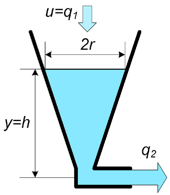
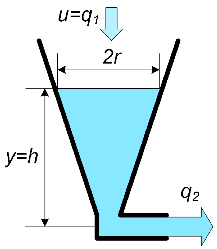
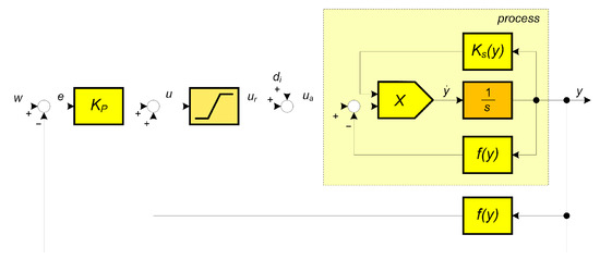
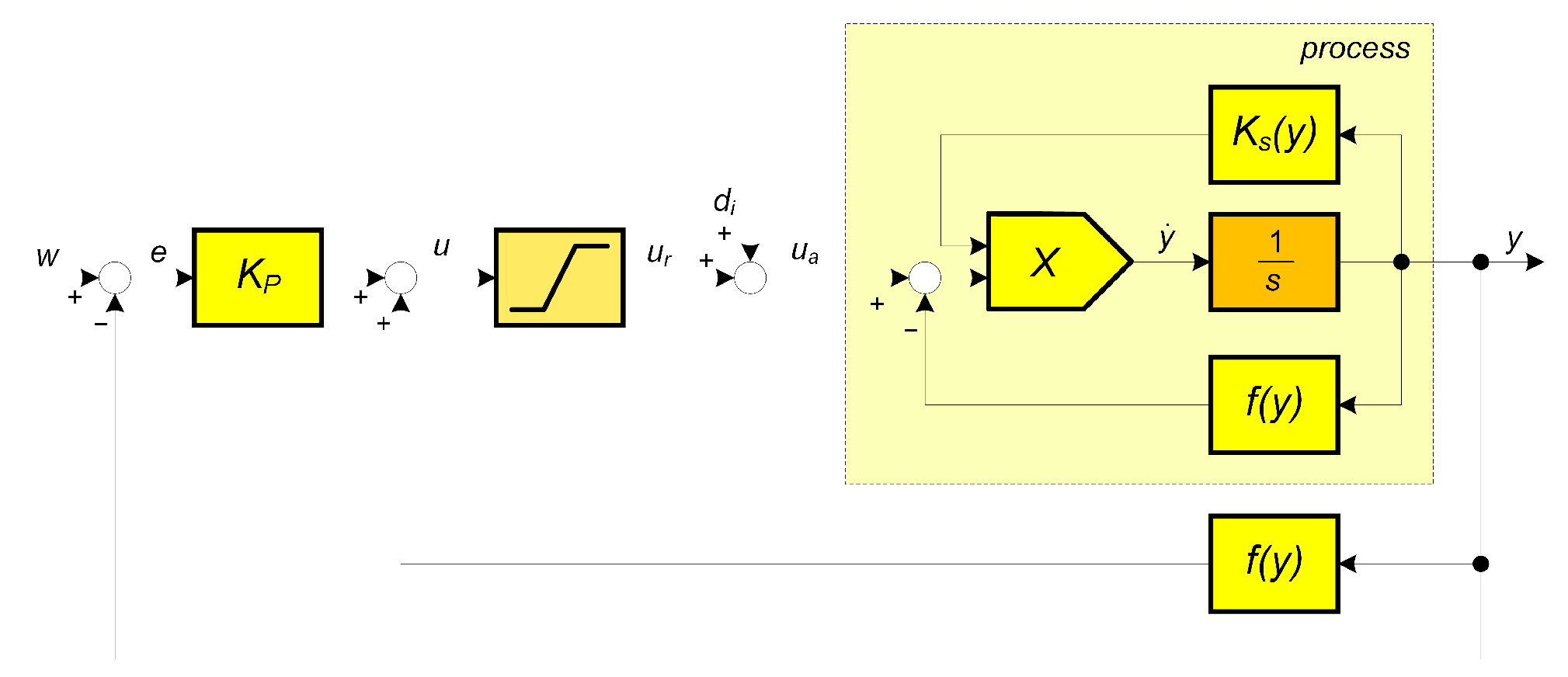
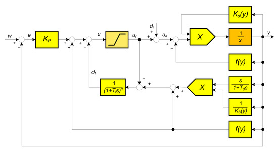
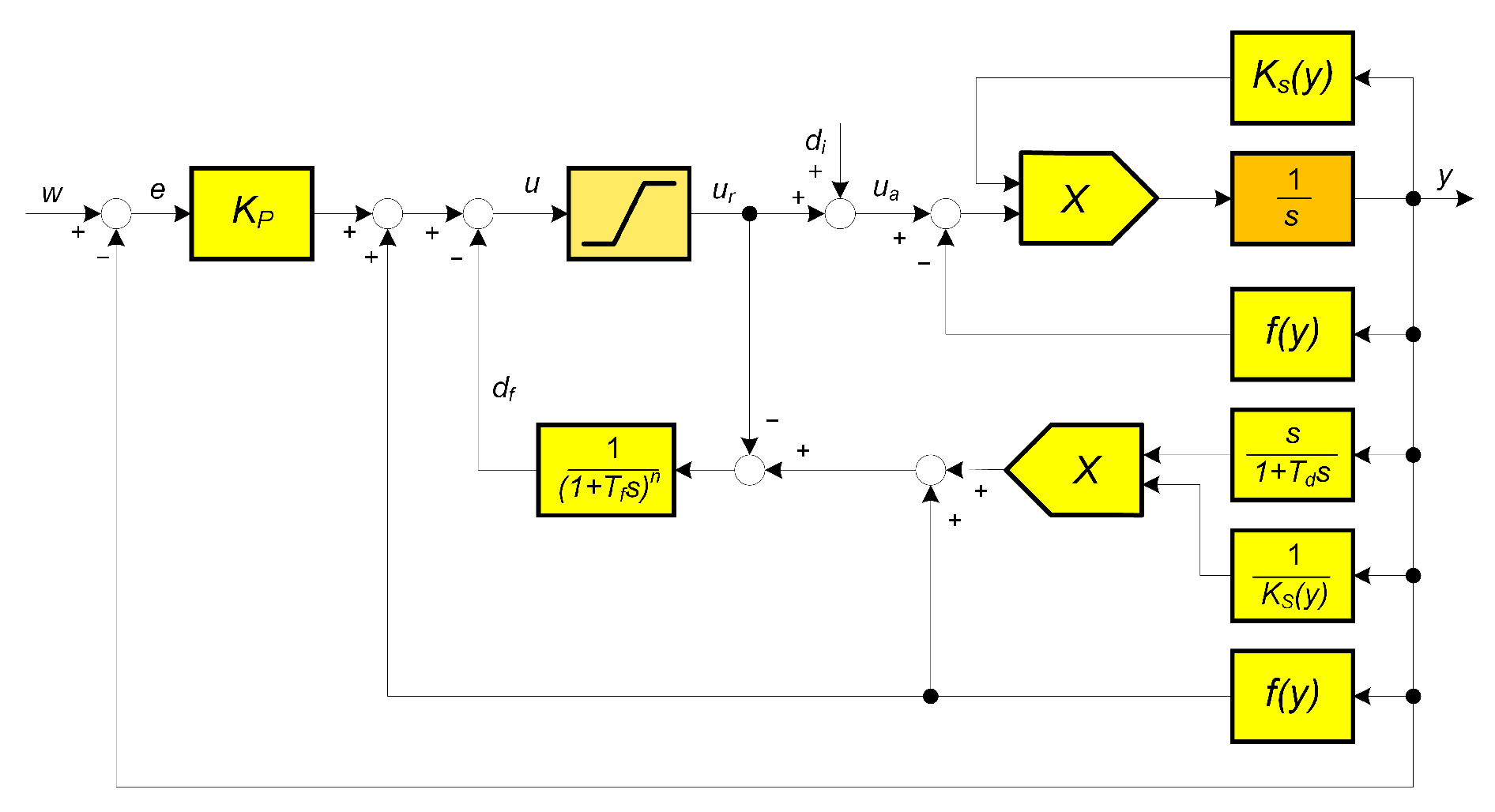
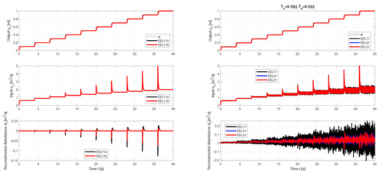
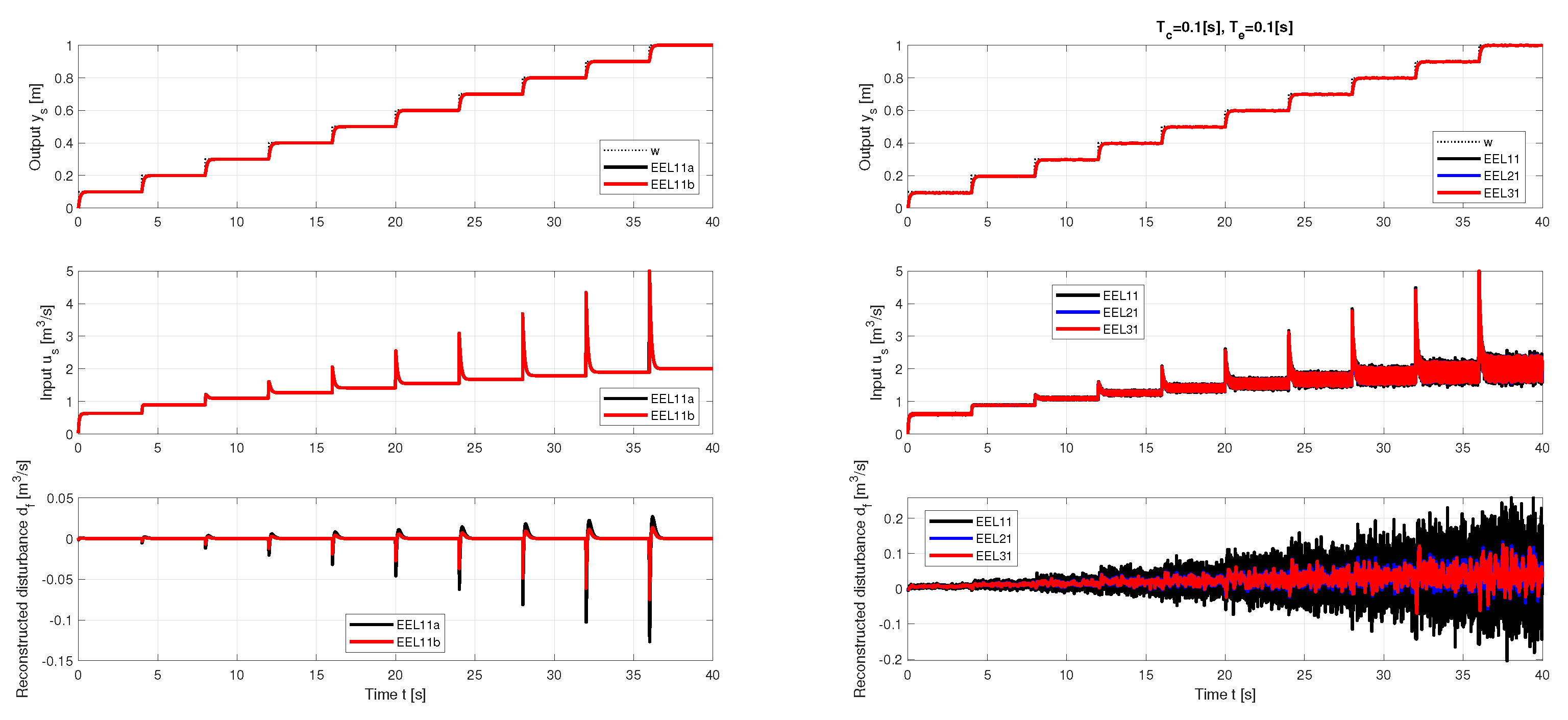
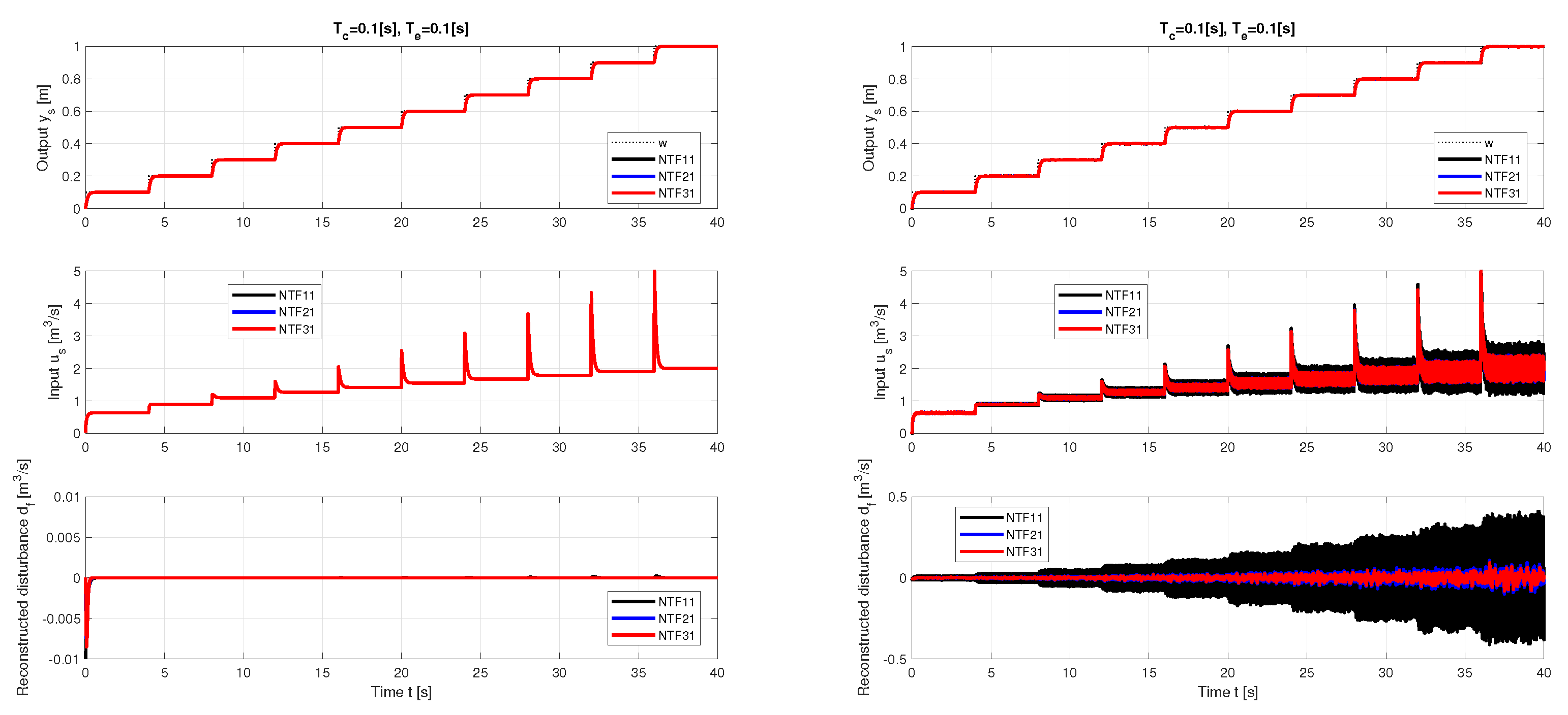
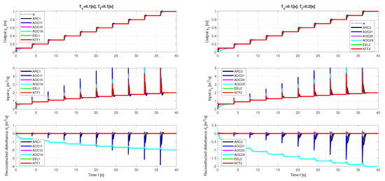
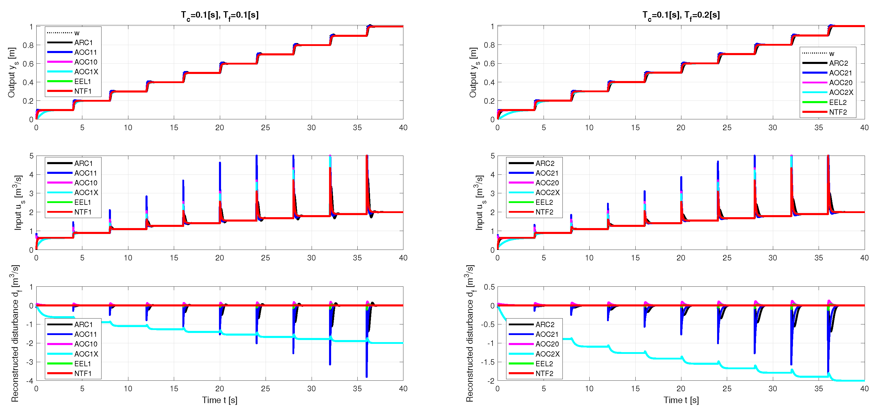
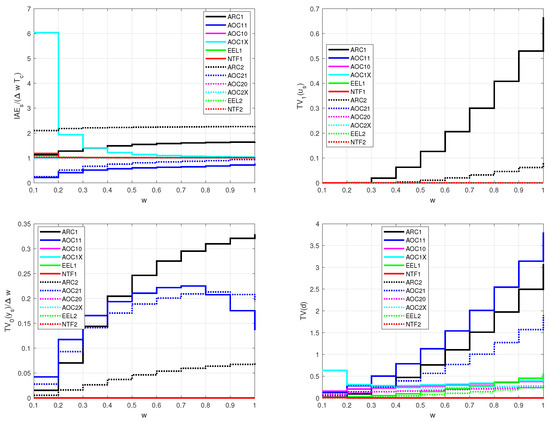
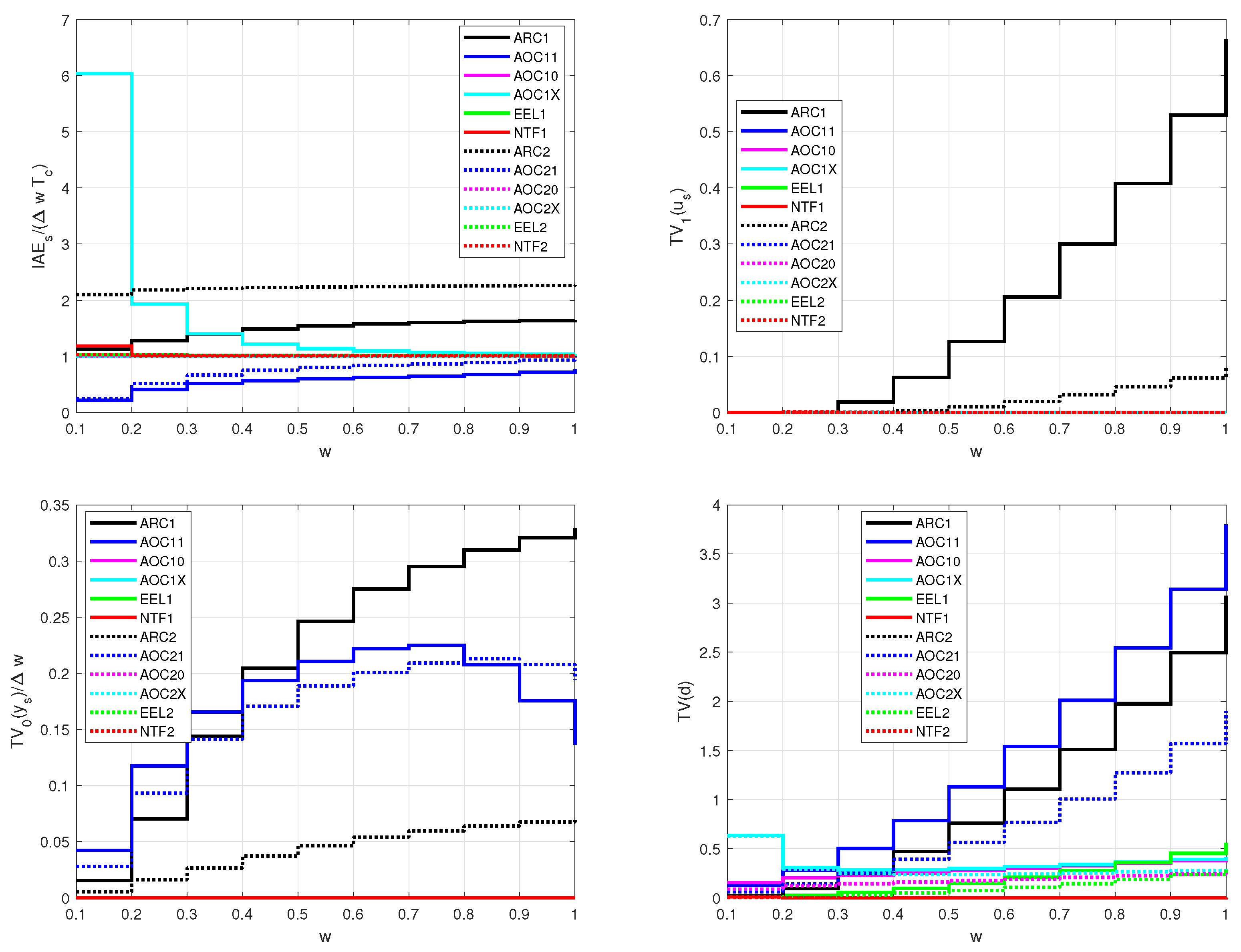
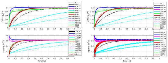
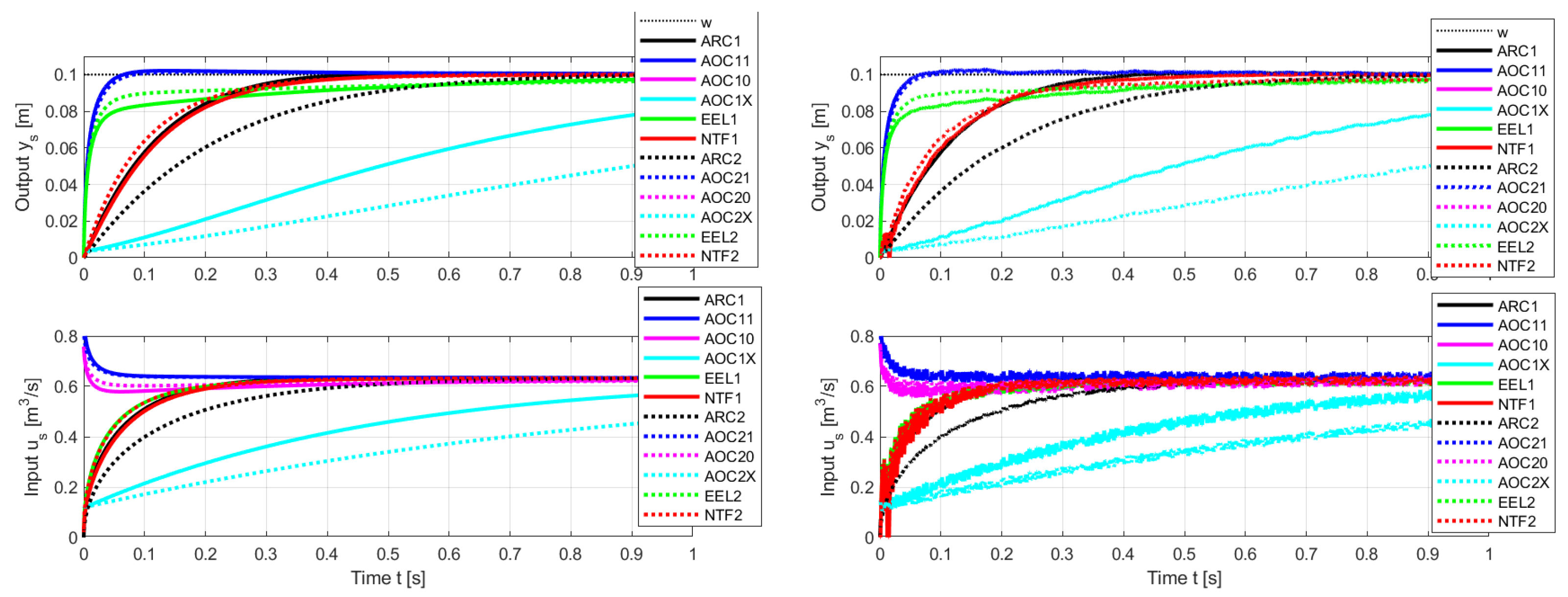
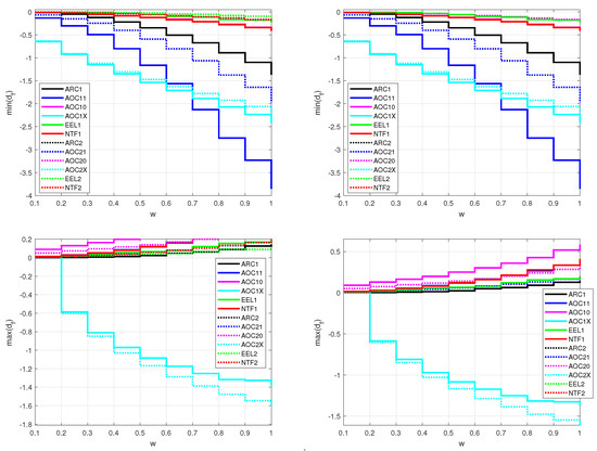
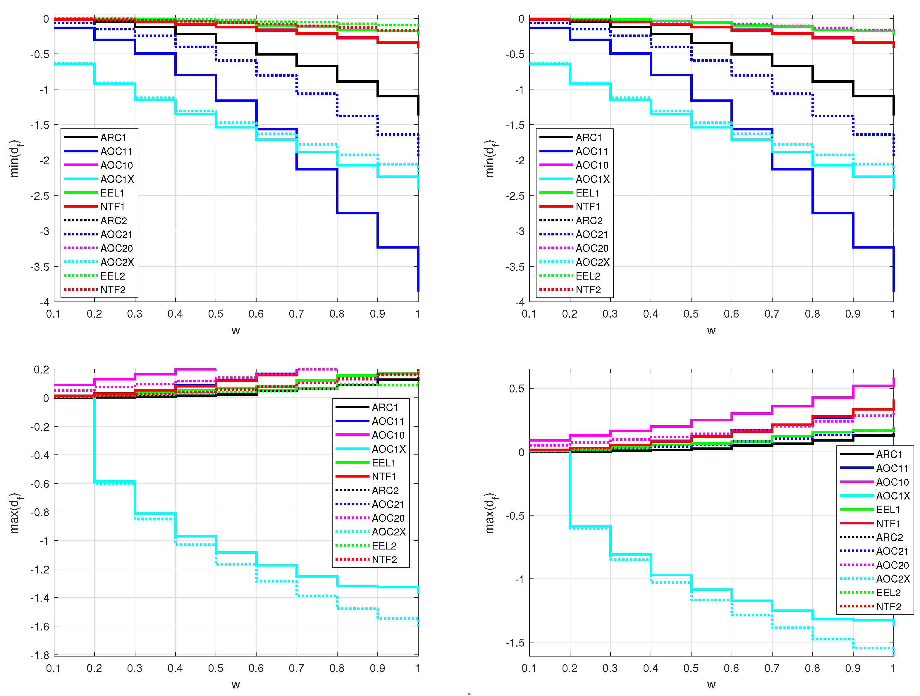
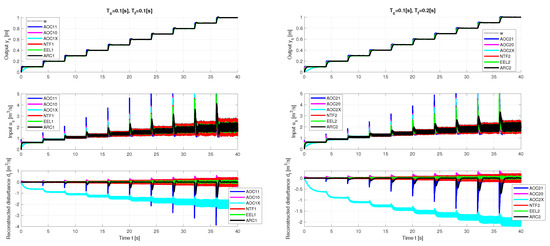
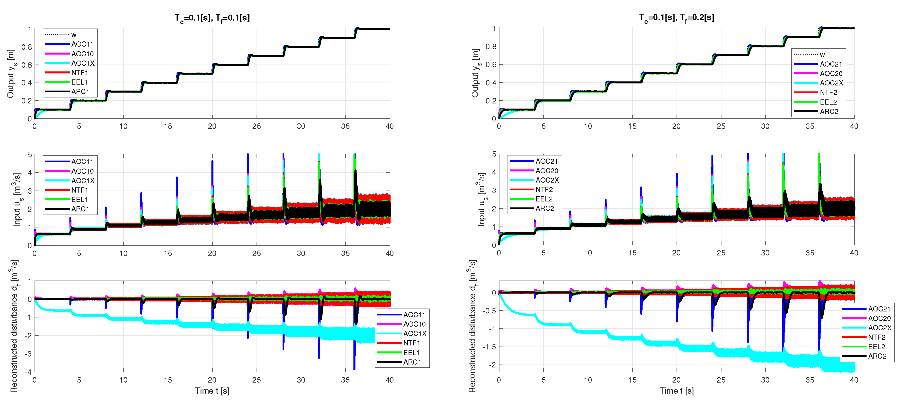
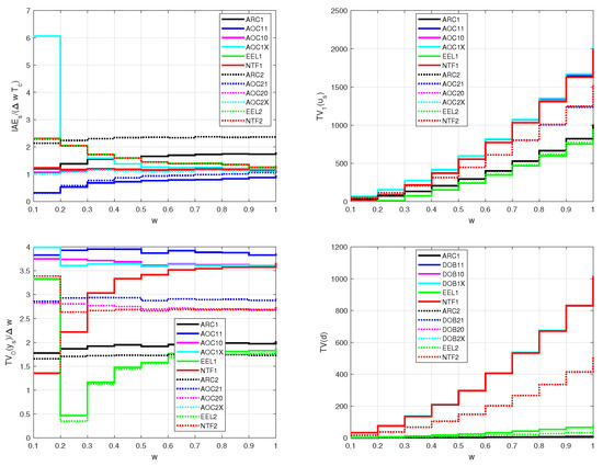
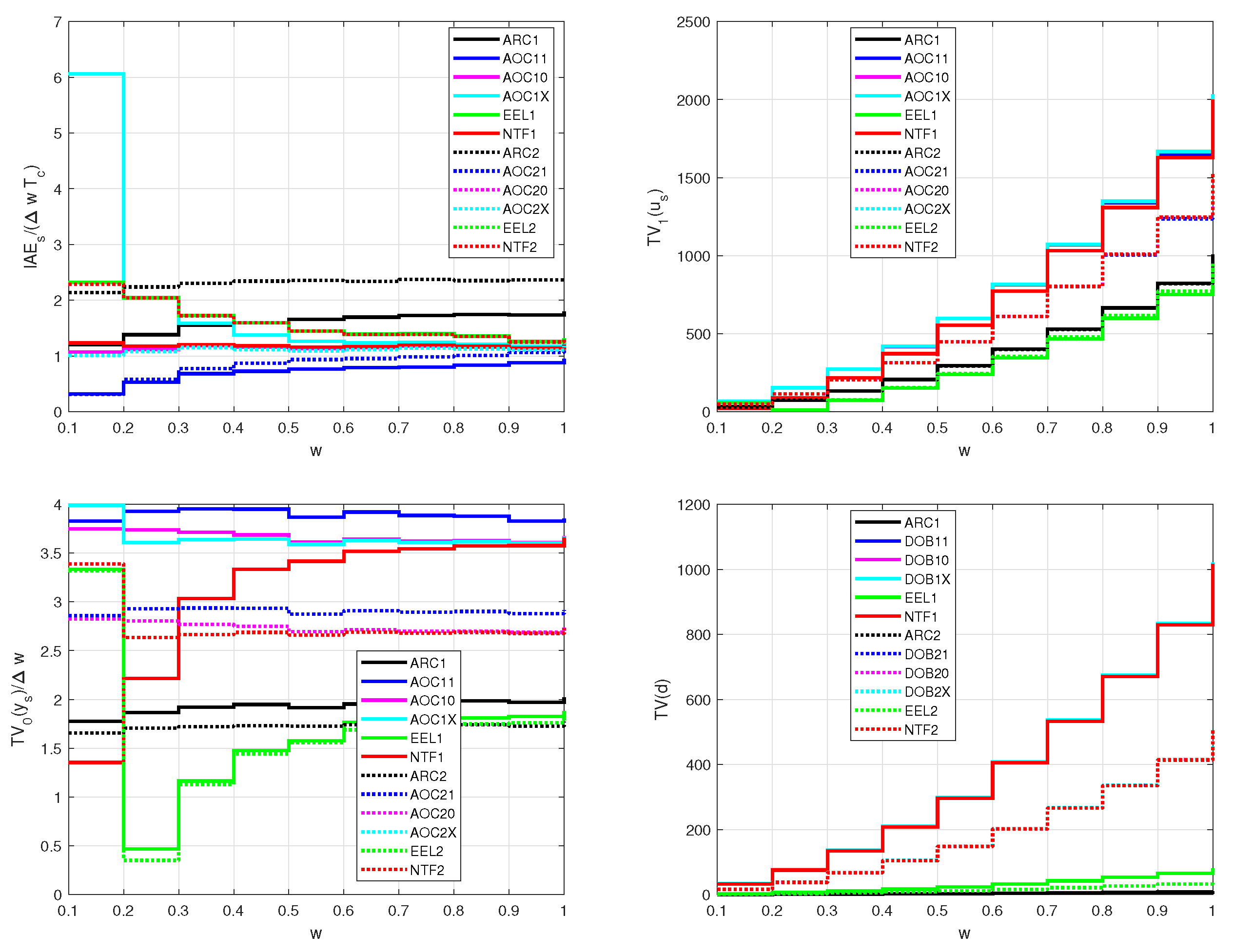
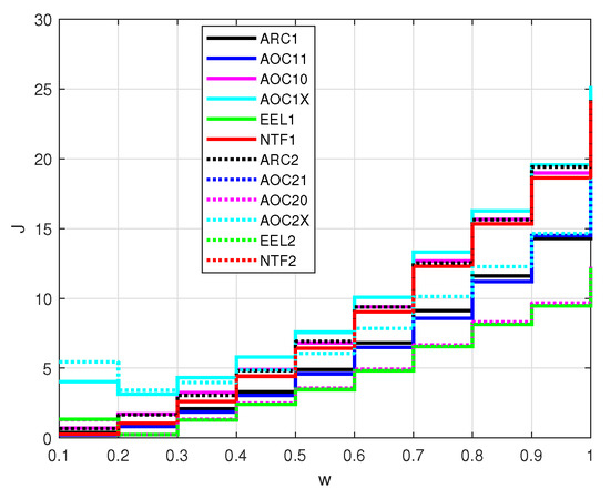
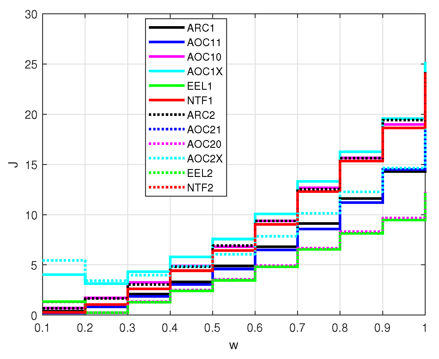
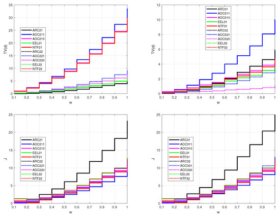
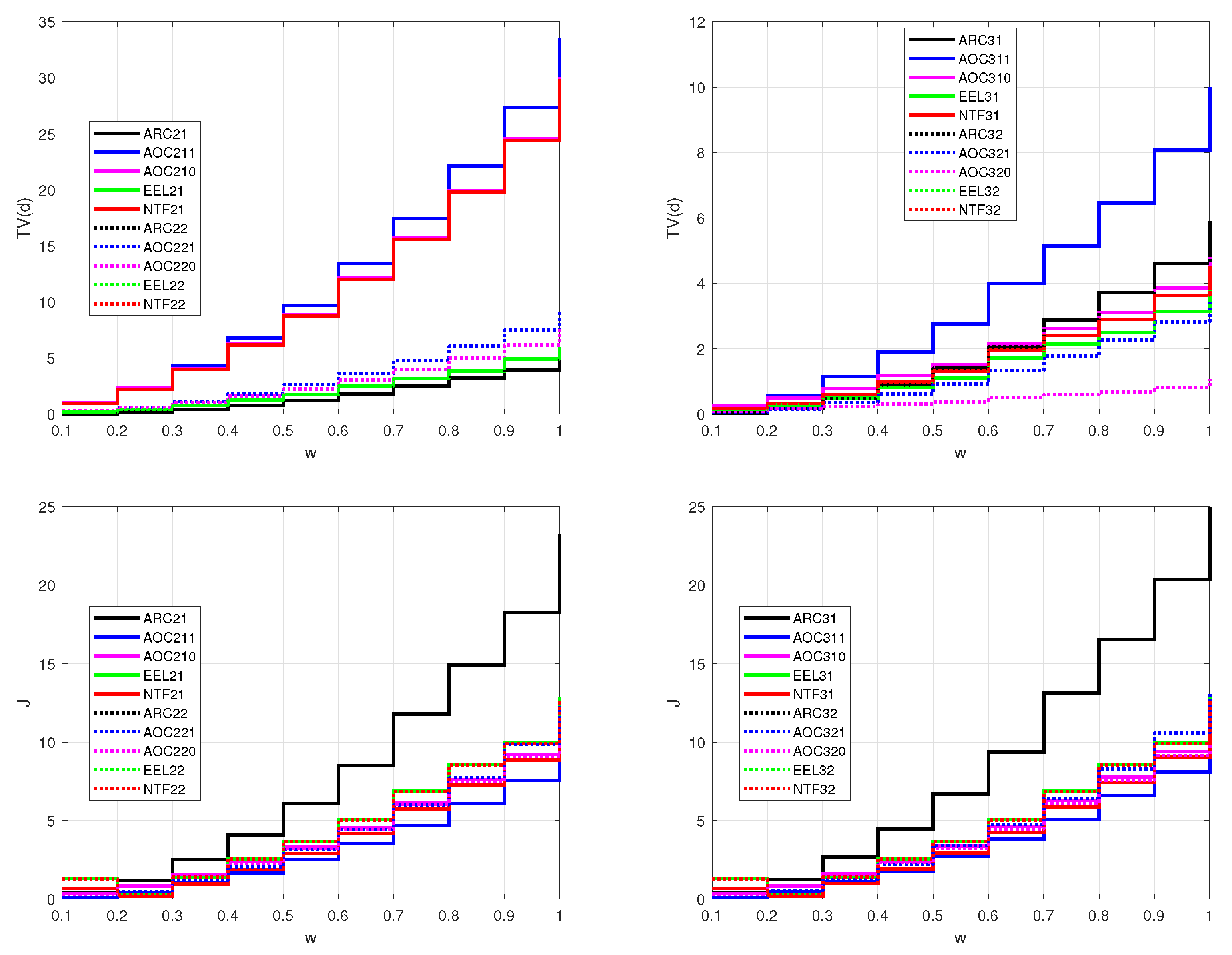
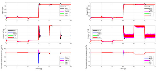
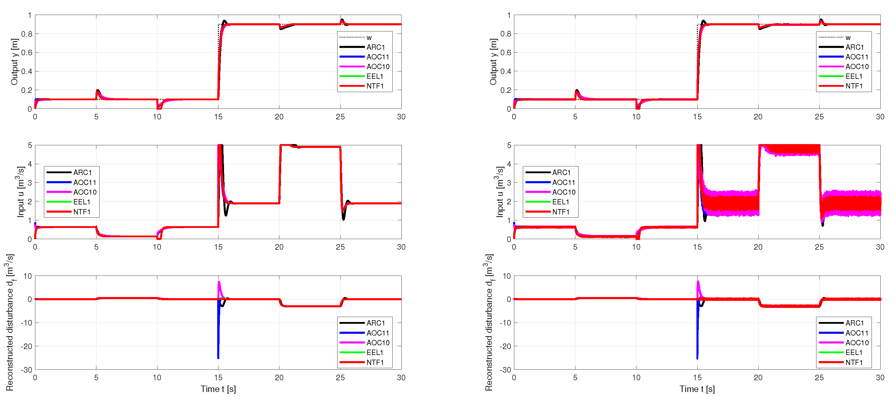
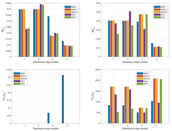
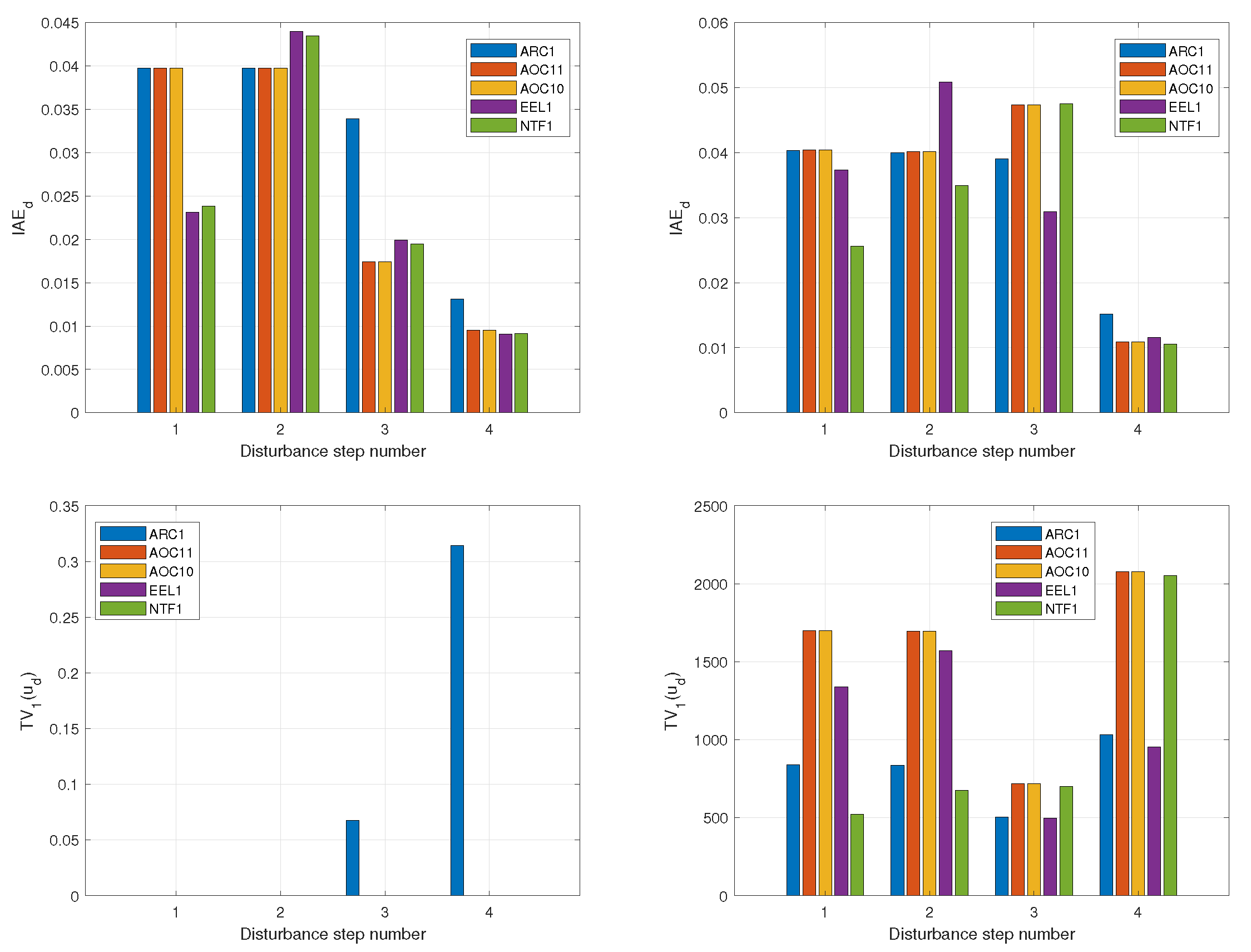
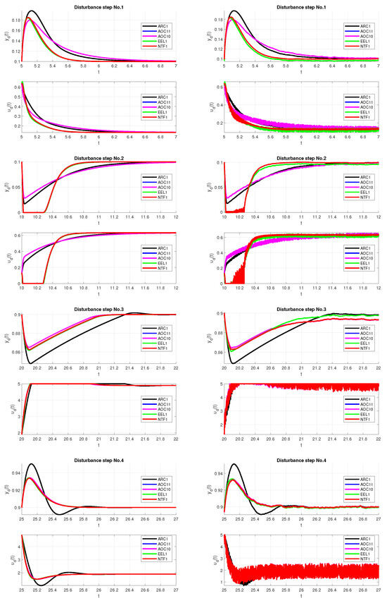
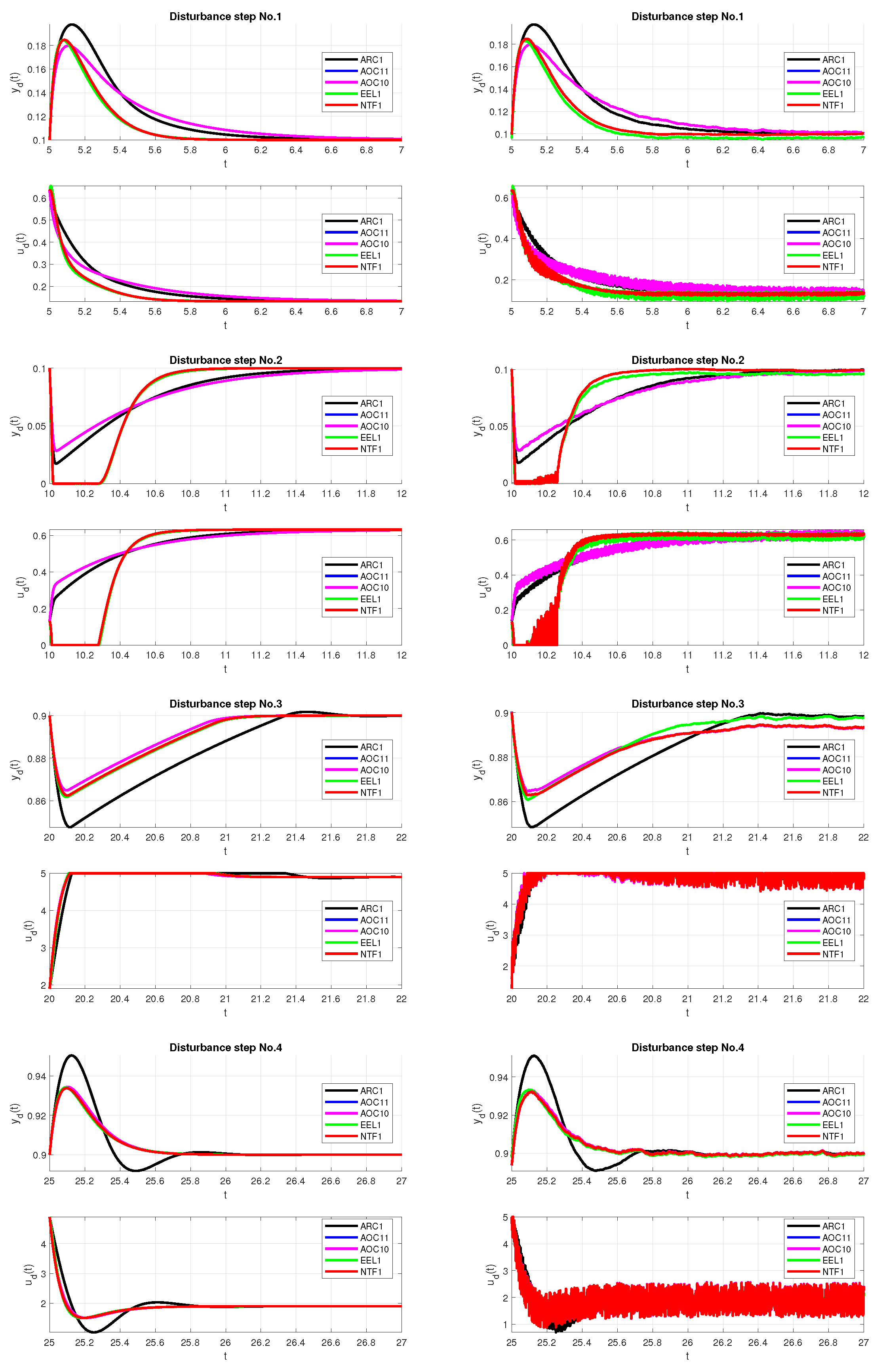

Disclaimer/Publisher’s Note: The statements, opinions and data contained in all publications are solely those of the individual author(s) and contributor(s) and not of MDPI and/or the editor(s). MDPI and/or the editor(s) disclaim responsibility for any injury to people or property resulting from any ideas, methods, instructions or products referred to in the content. |
© 2026 by the authors. Licensee MDPI, Basel, Switzerland. This article is an open access article distributed under the terms and conditions of the Creative Commons Attribution (CC BY) license.