Three Algebraic Conjugates with Zero Sum: A Graph-Theoretic Approach

Abstract

We give an alternative graph-theoretic proof that 20 is the least degree not divisible by 3 of an algebraic number having three distinct conjugates with zero sum. The proof excludes degree 16 through local constraints on vertex-transitive graphs of valency 6. The underlying graph construction can be studied in arbitrary degree, without the special degree restrictions of our group-theoretic arguments.

1. Introduction

Let $\alpha$ be an algebraic number of degree d over $\mathbb{Q}$, and suppose that three distinct algebraic conjugates ${\alpha }_1,{\alpha }_2,{\alpha }_3$ of $\alpha$ satisfy ${\alpha }_1+{\alpha }_2+{\alpha }_3=0$. In 2004, Dubickas and Smyth [1] asked whether d must be divisible by 3. Stong constructed a counterexample of degree 20: the irreducible polynomial

$$x^{20}+4·5^9{x}^{10}+16·5^{15}$$

has three distinct roots whose sum is zero (see [1]). This raises the natural question of determining the least degree d not divisible by 3 for which such a relation can occur. Recently, we established the following result:

Theorem 1 

([2] (to appear in Proc. Am. Math. Soc.)). Let $d>1$ be the smallest positive integer not a multiple of 3 for which there exists an algebraic number of degree d whose three algebraic conjugates sum to zero. Then $d=20$.

The relation among three conjugates is a special case of

$$a_1{\alpha }_1+a_2{\alpha }_2+\cdots +a_d{\alpha }_d=0,$$

(1)

where ${\alpha }_1,\dots ,{\alpha }_d$ are the conjugates of an algebraic number of degree d and $a_1,\dots ,a_d\in \mathbb{Z}$ are not all zero. Such a relation is called trivial when $a_1=\cdots =a_d$. For prime d, Kurbatov proved that every such relation is trivial [3]; related foundational results appear in [4,5], and Girstmair developed a representation-theoretic framework for the general problem [6]. Sparse additive relations have subsequently been studied in [7,8,9,10,11,12,13,14,15,16,17], with a multiplicative analogue considered in [18].

This paper develops the graph-theoretic proof introduced in [19], giving an alternative proof of Theorem 1. In the remaining case $d=16$, zero-sum triples yield a Galois-invariant linear 3-uniform hypergraph and a vertex-transitive graph of valency 6. Local constraints on its triangles reduce the arithmetic problem to explicit exclusions within the census of 40 such graphs [20,21].

Our group-theoretic arguments in [2] apply to the special degree families $d=p^m$ and $d=2p^m$: they exclude zero-sum triples when $p\ne 3$ in the first family and $p\ge 5$ in the second, where p is prime and $m\ge 1$. These arguments use the corresponding orbit structure of Sylow subgroups. The graph construction has no such restriction on the degree and can, in principle, be studied for arbitrary d. Proposition 1 supplies the general incidence constraints, while the degree-16 analysis illustrates how the local restrictions in Lemma 8 can be combined with finite census computations. This formulation allows the structural arguments and the explicit graph witnesses to be checked separately.

Section 2 collects the auxiliary results, and Section 3 gives the proof of Theorem 1. Appendix A specifies the complete executable verification script, census data, and recorded output supplied with this manuscript.

2. Auxiliary Results

The first general result related to linear relations among algebraic conjugates of a given algebraic number was obtained by Kurbatov [3]:

Lemma 1. 

The equality

$$k_1{\alpha }_1+k_2{\alpha }_2+\cdots +k_d{\alpha }_d=0$$

with conjugates ${\alpha }_1,{\alpha }_2,\dots ,{\alpha }_d$ of an algebraic number α of prime degree d over $\mathbb{Q}$ and $k_1,k_2,\dots ,k_d\in \mathbb{Z}$ can only hold if $k_1=k_2=\cdots =k_d$.

The result of Smyth [22] will be used several times in the proof of Theorem 1 to eliminate impossible relations among algebraic conjugates:

Lemma 2. 

If ${\alpha }_1,{\alpha }_2,{\alpha }_3$ are three conjugates of an algebraic number satisfying ${\alpha }_1\ne {\alpha }_2$, then $2{\alpha }_1\ne {\alpha }_2+{\alpha }_3$.

Dubickas [23] (see also [5], Theorem 3’) generalized Lemma 2 as follows:

Lemma 3. 

If ${\alpha }_1,{\alpha }_2,\dots ,{\alpha }_d$, where $d⩾3$, are distinct algebraic numbers conjugate over a field K of characteristic zero, and $k_1,k_2,\dots ,k_d$ are non-zero rational numbers satisfying $|k_1|⩾|k_2|+\cdots +|k_d|$, then

$$k_1{\alpha }_1+k_2{\alpha }_2+\cdots +k_d{\alpha }_d\notin K.$$

Also, we will use the result proved by Dubickas and Jankauskas [14].

Lemma 4. 

The equality

$$k_1{\alpha }_1+k_2{\alpha }_2+\cdots +k_d{\alpha }_d=0$$

with conjugates ${\alpha }_1,{\alpha }_2,\dots ,{\alpha }_d$ of an algebraic number α of degree d over $\mathbb{Q}$ and $k_1,k_2,\dots ,k_d\in \mathbb{Z}$ satisfying ${\sum }_{i=1}^d{k}_i\ne 0$ can only hold if $tr\left(\alpha \right):={\alpha }_1+{\alpha }_2+\cdots +{\alpha }_d=0$.

3. Proof of Theorem 1

Proof. 

Let d be a positive integer not divisible by 3. Let $\alpha$ be an algebraic number over $\mathbb{Q}$ of degree d whose three algebraic conjugates sum to zero. Suppose that d is the smallest possible such positive integer.

By the example of Stong [1], $d⩽20$. Dubickas and Jankauskas proved that $d⩾10$ (see Theorem 1.2 in [14]). By Lemma 1, d cannot be a prime number. Thus $d\in \{10,14,16,20\}$. Recently, Virbalas eliminated the cases $d=10$ and $d=14$ by proving that $d\ne 2p$, where $p⩾5$ is a prime number (see Theorem 1.1 in [24]). So $d=16$ or $d=20$. Our goal is to show that $d\ne 16$. This will establish that $d=20$.

Assume, to the contrary, that there exists an algebraic number $\alpha$ of degree $d=16$ whose algebraic conjugates ${\alpha }_1,{\alpha }_2,{\alpha }_3$ satisfy the relation

$${\alpha }_1+{\alpha }_2+{\alpha }_3=0.$$

(2)

Clearly, these three conjugates cannot all be equal. Moreover, if some two conjugates are equal, say ${\alpha }_1={\alpha }_2$, then $2{\alpha }_1+{\alpha }_3=0$, which is impossible (we can choose an automorphism $\pi$ in the Galois group of the normal closure of $\mathbb{Q}\left(\alpha \right)$ which maps ${\alpha }_1$ to ${\alpha }^{\prime }$ having the maximal absolute value m; then $2{\alpha }_1+{\alpha }_3=0$ is mapped to $2{\alpha }^{\prime }+\pi \left({\alpha }_3\right)=0$ and $2m=|2{\alpha }^{\prime }|=|-\pi \left({\alpha }_3\right)|⩽m$, which is impossible). Hence, all three conjugates in (2) are distinct.

Let ${\alpha }_1,{\alpha }_2,\dots ,{\alpha }_{16}$ be the algebraic conjugates of $\alpha$. Lemma 4 implies that $tr\left(\alpha \right)={\alpha }_1+{\alpha }_2+\cdots +{\alpha }_{16}=0$. Let G be the Galois group of the normal closure of $\mathbb{Q}\left(\alpha \right)$ over $\mathbb{Q}$. Note that this normal closure is also the splitting field of the minimal polynomial of $\alpha$ over $\mathbb{Q}$, and therefore G is the Galois group of this polynomial. The group G corresponds to some transitive subgroup of the full symmetric group $S_{16}$.

Two relations ${\alpha }_i+{\alpha }_j+{\alpha }_k=0$ and ${\alpha }_{i^{\prime }}+{\alpha }_{j^{\prime }}+{\alpha }_{k^{\prime }}=0$, where all the summands are algebraic conjugates of $\alpha$, are called distinct if

$$\{{\alpha }_i,{\alpha }_j,{\alpha }_k\}\ne \{{\alpha }_{i^{\prime }},{\alpha }_{j^{\prime }},{\alpha }_{k^{\prime }}\}.$$

Lemma 5. 

For any two distinct relations ${\alpha }_i+{\alpha }_j+{\alpha }_k=0$ and ${\alpha }_{i^{\prime }}+{\alpha }_{j^{\prime }}+{\alpha }_{k^{\prime }}=0$, we have $|\{i,j,k\}\cap \{i^{\prime },j^{\prime },k^{\prime }\}|⩽1$.

Proof. 

Since the relations are distinct, we have that $|\{i,j,k\}\cap \{i^{\prime },j^{\prime },k^{\prime }\}|⩽2$. On the other hand, if, say, $\{j,k\}=\{j^{\prime },k^{\prime }\}$, then ${\alpha }_i=-{\alpha }_j-{\alpha }_k=-{\alpha }_{j^{\prime }}-{\alpha }_{k^{\prime }}={\alpha }_{i^{\prime }}$. Since the conjugates are distinct, $i=i^{\prime }$, so the two relations coincide, a contradiction. Hence, the claim follows.    □

Lemma 6. 

For any fixed $i_0\in \{1,2,\dots ,16\}$, the number of distinct relations of the form ${\alpha }_{i_0}+{\alpha }_j+{\alpha }_k=0$ is less than 6.

Proof. 

Assume, to the contrary, that for a fixed $i_0$ there exist six distinct relations of the form ${\alpha }_{i_0}+{\alpha }_j+{\alpha }_k=0$. Lemma 5 implies that for any two distinct relations ${\alpha }_{i_0}+{\alpha }_{j_1}+{\alpha }_{k_1}=0$ and ${\alpha }_{i_0}+{\alpha }_{j_2}+{\alpha }_{k_2}=0$ the sets $\{j_1,k_1\}$ and $\{j_2,k_2\}$ are disjoint. Without loss of generality, we consider the following six relations (after relabeling the conjugates of $\alpha$, if necessary):

$$\begin{array}{c}{\alpha }_1+{\alpha }_2+{\alpha }_3=0,\hfill \\ {\alpha }_1+{\alpha }_4+{\alpha }_5=0,\hfill \\ {\alpha }_1+{\alpha }_6+{\alpha }_7=0,\hfill \\ {\alpha }_1+{\alpha }_8+{\alpha }_9=0,\hfill \\ {\alpha }_1+{\alpha }_{10}+{\alpha }_{11}=0,\hfill \\ {\alpha }_1+{\alpha }_{12}+{\alpha }_{13}=0.\hfill \end{array}$$

By adding all of them and using $tr\left(\alpha \right)=0$, we obtain

$$6{\alpha }_1+{\alpha }_2+{\alpha }_3+\cdots +{\alpha }_{13}=5{\alpha }_1-{\alpha }_{14}-{\alpha }_{15}-{\alpha }_{16}=0,$$

which is impossible by Lemma 3.    □

We say that two relations ${\alpha }_i+{\alpha }_j+{\alpha }_k=0$ and ${\alpha }_{i^{\prime }}+{\alpha }_{j^{\prime }}+{\alpha }_{k^{\prime }}=0$ are conjugate if there exists an automorphism $\pi \in G$ such that

$$\{{\alpha }_i,{\alpha }_j,{\alpha }_k\}=\{\pi \left({\alpha }_{i^{\prime }}\right),\pi \left({\alpha }_{j^{\prime }}\right),\pi \left({\alpha }_{k^{\prime }}\right)\}.$$

One can easily see that this conjugacy relation is an equivalence relation on the set of all possible relations of the form ${\alpha }_i+{\alpha }_j+{\alpha }_k=0$.

Lemma 7. 

The following statements are true.

   (i)

Any two relations of the form ${\alpha }_i+{\alpha }_j+{\alpha }_k=0$ are conjugate.

  (ii)

There are exactly 16 distinct such relations.

 (iii)

Each algebraic conjugate of α appears in exactly 3 distinct such relations.

Proof. 

Consider a relation ${\alpha }_i+{\alpha }_j+{\alpha }_k=0$ and its equivalence class $\mathcal{C}({\alpha }_i,{\alpha }_j,{\alpha }_k)$, consisting of all the distinct relations that are conjugate to ${\alpha }_i+{\alpha }_j+{\alpha }_k=0$. Let $N=\left|\mathcal{C}\right({\alpha }_i,{\alpha }_j,{\alpha }_k\left)\right|$. Since the Galois group G acts transitively on the set $\{{\alpha }_1,{\alpha }_2,\dots ,{\alpha }_{16}\}$, each conjugate ${\alpha }_i$ appears an equal number of times, say l, in the relations in $\mathcal{C}({\alpha }_i,{\alpha }_j,{\alpha }_k)$. We have N distinct relations in $\mathcal{C}({\alpha }_i,{\alpha }_j,{\alpha }_k)$ and each such relation involves three distinct conjugates of $\alpha$. Thus, there are $3N$ appearances of conjugates of $\alpha$ in $\mathcal{C}({\alpha }_i,{\alpha }_j,{\alpha }_k)$. On the other hand, this number can be counted in a different way — each conjugate of $\alpha$ appears exactly l times. Hence, $3N=16l$. Since the class is nonempty and G acts transitively, $l>0$. As $\gcd (3,16)=1$, we have $3\mid l$. Lemma 6 gives $l<6$, so $l=3$ and $N=16$.

Assume that there are two distinct equivalence classes. Each contains three distinct relations involving ${\alpha }_1$. Thus, in total, we have six distinct relations involving ${\alpha }_1$. This contradicts Lemma 6. Hence, the lemma follows.    □

By Lemma 7, we have exactly 16 distinct relations of the form ${\alpha }_i+{\alpha }_j+{\alpha }_k=0$ and each ${\alpha }_i$ appears in exactly 3 distinct such relations. Without loss of generality, we assume the following system of distinct relations:

$$\begin{array}{cccccc}{\alpha }_1\hfill & +\hfill & {\alpha }_2\hfill & +\hfill & {\alpha }_3\hfill & =0,\\ {\alpha }_1\hfill & +\hfill & {\alpha }_4\hfill & +\hfill & {\alpha }_5\hfill & =0,\\ {\alpha }_1\hfill & +\hfill & {\alpha }_6\hfill & +\hfill & {\alpha }_7\hfill & =0,\\ {\alpha }_{i_{41}}\hfill & +\hfill & {\alpha }_{i_{42}}\hfill & +\hfill & {\alpha }_{i_{43}}\hfill & =0,\\ {\alpha }_{i_{51}}\hfill & +\hfill & {\alpha }_{i_{52}}\hfill & +\hfill & {\alpha }_{i_{53}}\hfill & =0,\\ & ⋮\hfill & & ⋮\hfill & & ⋮\hfill \\ {\alpha }_{i_{161}}\hfill & +\hfill & {\alpha }_{i_{162}}\hfill & +\hfill & {\alpha }_{i_{163}}\hfill & =0.\end{array}$$

(3)

This system of relations is equivalent to the following one:

$$\begin{array}{ccccccccccccc}-{\alpha }_1\hfill & =\hfill & {\alpha }_2\hfill & +\hfill & {\alpha }_3\hfill & =\hfill & {\alpha }_4\hfill & +\hfill & {\alpha }_5\hfill & =\hfill & {\alpha }_6\hfill & +\hfill & {\alpha }_7,\hfill \\ -{\alpha }_2\hfill & =\hfill & {\alpha }_1\hfill & +\hfill & {\alpha }_3\hfill & =\hfill & {\alpha }_{j_{23}}\hfill & +\hfill & {\alpha }_{j_{24}}\hfill & =\hfill & {\alpha }_{j_{25}}\hfill & +\hfill & {\alpha }_{j_{26}},\hfill \\ -{\alpha }_3\hfill & =\hfill & {\alpha }_1\hfill & +\hfill & {\alpha }_2\hfill & =\hfill & {\alpha }_{j_{33}}\hfill & +\hfill & {\alpha }_{j_{34}}\hfill & =\hfill & {\alpha }_{j_{35}}\hfill & +\hfill & {\alpha }_{j_{36}},\hfill \\ -{\alpha }_4\hfill & =\hfill & {\alpha }_1\hfill & +\hfill & {\alpha }_5\hfill & =\hfill & {\alpha }_{j_{43}}\hfill & +\hfill & {\alpha }_{j_{44}}\hfill & =\hfill & {\alpha }_{j_{45}}\hfill & +\hfill & {\alpha }_{j_{46}},\hfill \\ -{\alpha }_5\hfill & =\hfill & {\alpha }_1\hfill & +\hfill & {\alpha }_4\hfill & =\hfill & {\alpha }_{j_{53}}\hfill & +\hfill & {\alpha }_{j_{54}}\hfill & =\hfill & {\alpha }_{j_{55}}\hfill & +\hfill & {\alpha }_{j_{56}},\hfill \\ -{\alpha }_6\hfill & =\hfill & {\alpha }_1\hfill & +\hfill & {\alpha }_7\hfill & =\hfill & {\alpha }_{j_{63}}\hfill & +\hfill & {\alpha }_{j_{64}}\hfill & =\hfill & {\alpha }_{j_{65}}\hfill & +\hfill & {\alpha }_{j_{66}},\hfill \\ -{\alpha }_7\hfill & =\hfill & {\alpha }_1\hfill & +\hfill & {\alpha }_6\hfill & =\hfill & {\alpha }_{j_{73}}\hfill & +\hfill & {\alpha }_{j_{74}}\hfill & =\hfill & {\alpha }_{j_{75}}\hfill & +\hfill & {\alpha }_{j_{76}},\hfill \\ -{\alpha }_8\hfill & =\hfill & {\alpha }_{j_{81}}\hfill & +\hfill & {\alpha }_{j_{82}}\hfill & =\hfill & {\alpha }_{j_{83}}\hfill & +\hfill & {\alpha }_{j_{84}}\hfill & =\hfill & {\alpha }_{j_{85}}\hfill & +\hfill & {\alpha }_{j_{86}},\hfill \\ & ⋮\hfill & & & & ⋮\hfill & & & & ⋮\hfill & & & \\ -{\alpha }_{16}\hfill & =\hfill & {\alpha }_{j_{161}}\hfill & +\hfill & {\alpha }_{j_{162}}\hfill & =\hfill & {\alpha }_{j_{163}}\hfill & +\hfill & {\alpha }_{j_{164}}\hfill & =\hfill & {\alpha }_{j_{165}}\hfill & +\hfill & {\alpha }_{j_{166}}.\hfill \end{array}$$

(4)

Note that $-{\alpha }_1,-{\alpha }_2,\dots ,-{\alpha }_{16}$ are the algebraic conjugates of $-{\alpha }_1$. Since ${\alpha }_1+{\alpha }_2=-{\alpha }_3$ and $\mathbb{Q}(-{\alpha }_3)=\mathbb{Q}\left({\alpha }_3\right)$, we have $\mathrm{deg}({\alpha }_1+{\alpha }_2)=16$. Each sum ${\alpha }_i+{\alpha }_j$ appearing in (4) is therefore an algebraic conjugate of ${\alpha }_1+{\alpha }_2$.

Note that each algebraic conjugate of ${\alpha }_1+{\alpha }_2$ has exactly three distinct representations as a sum ${\alpha }_i+{\alpha }_j$ (see $\left(iii\right)$ in Lemma 7).

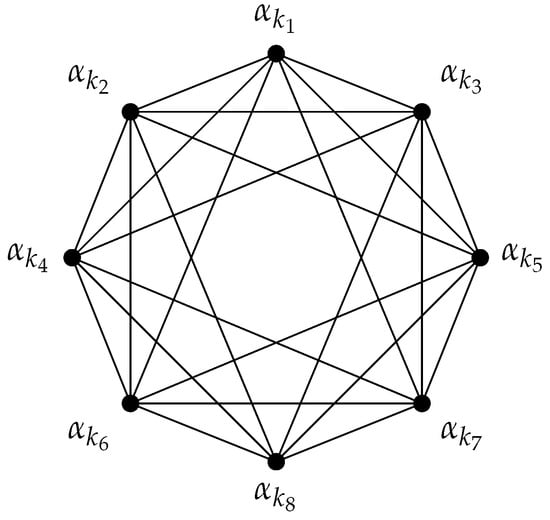
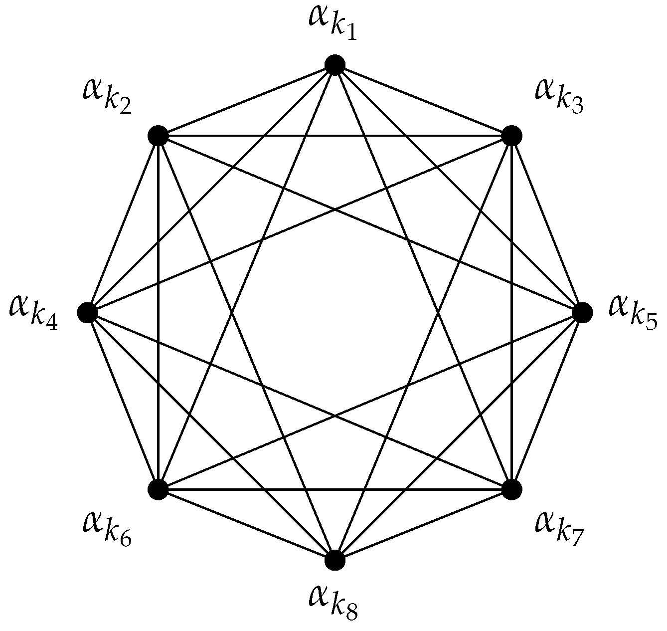
Now, we will introduce the graph-theoretic approach to this problem. Let $\mathcal{G}=(V,E)$ be the finite simple undirected graph with $V:=\{{\alpha }_1,\dots ,{\alpha }_{16}\}$. For $i\ne j$, the vertices ${\alpha }_i$ and ${\alpha }_j$ are joined by an edge, denoted $({\alpha }_i,{\alpha }_j)$ or $({\alpha }_j,{\alpha }_i)$, if ${\alpha }_i+{\alpha }_j$ is a conjugate of ${\alpha }_1+{\alpha }_2$, equivalently, if this sum appears in (4).

Note that each vertex of $\mathcal{G}$ must have the same number of edges. In other words, the graph $\mathcal{G}$ is regular. This follows directly from the fact that each ${\alpha }_i$ appears exactly six times in (4) (or, equivalently, each ${\alpha }_i$ appears in three distinct relations ${\alpha }_i+{\alpha }_j+{\alpha }_k=0$ and each such relation implies two edges $({\alpha }_i,{\alpha }_j)$ and $({\alpha }_i,{\alpha }_k)$, connecting the vertex ${\alpha }_i$), i.e., $\mathrm{deg}\left(v\right)=6$ for each $v\in V$. In such a setting, $\mathcal{G}$ must have $(16·6)/2=48$ edges. Furthermore, since the Galois group G is transitive on the set of conjugates $\{{\alpha }_1,{\alpha }_2,\dots ,{\alpha }_{16}\}$ and, by Lemma 7, any two relations of the form ${\alpha }_i+{\alpha }_j+{\alpha }_k=0$ are conjugate, the graph $\mathcal{G}$ must be vertex-transitive. It is known that there are exactly 40 vertex-transitive graphs on 16 vertices of degree 6. This was established by McKay and Royle [20] in their complete enumeration of transitive graphs on at most 26 vertices. The explicit list is maintained in [21] (https://doi.org/10.5281/zenodo.4010122) (see also the House of Graphs [25]). All 40 of these graphs, named ${\mathcal{G}}_1,{\mathcal{G}}_2,\dots ,{\mathcal{G}}_{40}$, are given in Table 1. Note that these graphs are given in graph6 format (this format was invented by Brendan McKay [26,27] and is recognized by SageMath [28]).

Table 1. All 40 vertex-transitive graphs on 16 vertices of degree 6 (see [21]).

Graph	Code in graph6 Format
${\mathcal{G}}_1$	OsaC???FzrMkYwXwJw@|?
${\mathcal{G}}_2$	OsaC???RxnNKYw\WJs@}?
${\mathcal{G}}_3$	OsaC???]ZrK{XwFwB{B{?
${\mathcal{G}}_4$	OsaCB@_EWrKrXeFwB{B{?
${\mathcal{G}}_5$	OsaKYCQGbRIjXKLWJEHqc
${\mathcal{G}}_6$	OsaKYCcQXRBKSbLDmTBi_
${\mathcal{G}}_7$	OsaKYDDGgdLBUELQeibr?
${\mathcal{G}}_8$	OsaKYPDHOiDFEM[wMPRcg
${\mathcal{G}}_9$	OsaKg?dQGid\[S[qLSQy_
${\mathcal{G}}_{10}$	OsaKg?hSZEkkTIIdJWPyA
${\mathcal{G}}_{11}$	OsaKiCaC‘RbMYKTYLabiC
${\mathcal{G}}_{12}$	OsaKiCdPPDaUBR]WNAboS
${\mathcal{G}}_{13}$	OsaSWSTOhDKiXQUEfBbr?
${\mathcal{G}}_{14}$	OsaSXCdOha‘T[DRRNEAyC
${\mathcal{G}}_{15}$	OsaSXDCSXRbKTBIdmSBY@
${\mathcal{G}}_{16}$	OsaSYHBGpH‘XDL]SNDBoK
${\mathcal{G}}_{17}$	Osedw?DOYFHBSZW\Fg@w‘
${\mathcal{G}}_{18}$	Osedw?HOYFGbSZW\Fg@w‘
${\mathcal{G}}_{19}$	Osedw@??pJhMP\UWEjBpA
${\mathcal{G}}_{20}$	OsfDw?@G‘bgmW\RWFFAyA
${\mathcal{G}}_{21}$	OsfDw@@GXPCZP]TSFDayA
${\mathcal{G}}_{22}$	OsfLg?@WYHcZQYKXJcPuA
${\mathcal{G}}_{23}$	Osqsw@@AXCclW]USEXaxA
${\mathcal{G}}_{24}$	Osqsy@@GWRcdGtUEESqyA
${\mathcal{G}}_{25}$	OtaCXOTHOphhRKSsKTJcK
${\mathcal{G}}_{26}$	OtaLw?@OaRgn[S[Kdk?z@
${\mathcal{G}}_{27}$	OtaLw?@ObBiNQ[P[fg@x@
${\mathcal{G}}_{28}$	OtaLw?BOBBhNP[S[fa@y@
${\mathcal{G}}_{29}$	OtaLy@@AWJg[WFSFfg@x@
${\mathcal{G}}_{30}$	OtaLyD‘SYQGhKBKB‘eOXb
${\mathcal{G}}_{31}$	Ota\W@@GYChJS]PZFc@u@
${\mathcal{G}}_{32}$	Otakw?@QYbKLPLOufc@u@
${\mathcal{G}}_{33}$	Otaky@@GWbhBPROlfc@u@
${\mathcal{G}}_{34}$	OtrTOGBW@‘hIP]G|Bg_tP
${\mathcal{G}}_{35}$	Ouj\w?@?YBcMSUILIhPTI
${\mathcal{G}}_{36}$	O{fL_@HKQJCZCsBW_pzp_
${\mathcal{G}}_{37}$	O{fL_CCQP‘GmCzB[C\Joo
${\mathcal{G}}_{38}$	O}akqPPWOV@iHIDHcROcj
${\mathcal{G}}_{39}$	O~aKYPDOxQBHHIGeacocj
${\mathcal{G}}_{40}$	O~z\w?@?WB_M?Z?V_Fz{?

The goal is to prove that for every $i\in \{1,2,\dots 40\}$, the graphs $\mathcal{G}$ and ${\mathcal{G}}_i$ are not isomorphic.

Note that a relation ${\alpha }_i+{\alpha }_j+{\alpha }_k=0$ in (3) implies the three equalities ${\alpha }_i+{\alpha }_j=-{\alpha }_k,{\alpha }_i+{\alpha }_k=-{\alpha }_j$, and ${\alpha }_j+{\alpha }_k=-{\alpha }_i$. Thus, the three sums on the left are algebraic conjugates of ${\alpha }_1+{\alpha }_2=-{\alpha }_3$. In other words, edges $({\alpha }_i,{\alpha }_j),({\alpha }_i,{\alpha }_k)$, and $({\alpha }_j,{\alpha }_k)$ form a triangle in our graph $\mathcal{G}$. On the other hand, if, for three distinct conjugates ${\alpha }_a,{\alpha }_b,{\alpha }_c$, all three edges $({\alpha }_a,{\alpha }_b),({\alpha }_b,{\alpha }_c)$ and $({\alpha }_a,{\alpha }_c)$ belong to $\mathcal{G}$, then the relation ${\alpha }_a+{\alpha }_b+{\alpha }_c=0$ need not hold. If it does, then we say that the vertices ${\alpha }_a,{\alpha }_b,{\alpha }_c$ form a zero-sum triangle $▵({\alpha }_a,{\alpha }_b,{\alpha }_c)$.

Write ${\mathrm{deg}}_{\mathcal{G}}\left(v\right)$ for the degree of a vertex v in a graph $\mathcal{G}$, $N\left(v\right)$ for its open neighborhood, and $N\left[v\right]=N\left(v\right)\cup \left\{v\right\}$ for its closed neighborhood. The induced graph on a vertex set retains exactly the edges with both endpoints in that set. We denote the graph induced on $N\left[v\right]$ by $\mathcal{G}\left(v\right)$; degrees in $\mathcal{G}\left(v\right)$ are taken within this induced graph.

Lemma 8. 

The following statements are true for the graph $\mathcal{G}$.

   (i)

Two distinct zero-sum triangles share at most one vertex.

  (ii)

Every edge $(\alpha ,{\alpha }^{\prime })$, $\alpha \ne {\alpha }^{\prime }$, belongs to exactly one zero-sum triangle $▵(\alpha ,{\alpha }^{\prime },{\alpha }^{″})$ and the vertex ${\alpha }^{\prime \prime }$ belongs to the open neighborhood $N\left(\alpha \right)$ of α.

 (iii)

If $\alpha ,{\alpha }^{\prime },{\alpha }^{″}$ are three distinct vertices such that ${\alpha }^{\prime },{\alpha }^{″}\in N\left(\alpha \right)$, ${\mathrm{deg}}_{\mathcal{G}\left(\alpha \right)}\left({\alpha }^{\prime }\right)=2$ and $({\alpha }^{\prime },{\alpha }^{″})$ is an edge in $\mathcal{G}$, then $▵(\alpha ,{\alpha }^{\prime },{\alpha }^{″})$ is a zero-sum triangle.

 (iv)

If $▵(\alpha ,{\alpha }_a,{\alpha }_b)$ and $▵(\alpha ,{\alpha }_c,{\alpha }_d)$ are two distinct zero-sum triangles, then either $({\alpha }_a,{\alpha }_d)$ or $({\alpha }_b,{\alpha }_c)$ is not an edge in $\mathcal{G}$.

Proof. 

Part $\left(i\right)$ follows from the definition of the graph $\mathcal{G}$ and Lemma 5.

$\left(ii\right)$. Let $(\alpha ,{\alpha }^{\prime })$, $\alpha \ne {\alpha }^{\prime }$, be an edge in $\mathcal{G}$. Then, according to the definition of $\mathcal{G}$, the sum $\alpha +{\alpha }^{\prime }$ is an algebraic conjugate of ${\alpha }_1+{\alpha }_2=-{\alpha }_3$. Hence, $\alpha +{\alpha }^{\prime }=-{\alpha }^{″}$ for a conjugate ${\alpha }^{″}$. If ${\alpha }^{″}$ equaled either endpoint, we would obtain $2\beta +\gamma =0$ for conjugates $\beta ,\gamma$, which the maximal-absolute-value argument following (2) excludes. Thus, the three vertices are distinct, and $▵(\alpha ,{\alpha }^{\prime },{\alpha }^{″})$ is a zero-sum triangle. Part $\left(i\right)$ makes it the unique zero-sum triangle containing $(\alpha ,{\alpha }^{\prime })$. Moreover, $(\alpha ,{\alpha }^{″})$ is also an edge in $\mathcal{G}$, since $\alpha +{\alpha }^{″}=-{\alpha }^{\prime }$ is an algebraic conjugate of ${\alpha }_1+{\alpha }_2=-{\alpha }_3$. So ${\alpha }^{″}$ is adjacent to $\alpha$, ${\alpha }^{″}\ne \alpha$, and therefore ${\alpha }^{″}\in N\left(\alpha \right)$.

$\left(iii\right)$. Since ${\alpha }^{\prime }\in N\left(\alpha \right)$, we have that $(\alpha ,{\alpha }^{\prime })$ is an edge in $\mathcal{G}$. Applying part $\left(ii\right)$, we obtain that there exists a vertex $\tilde{\alpha }\in N\left(\alpha \right)$ such that the triangle $▵(\alpha ,{\alpha }^{\prime },\tilde{\alpha })$ is a zero-sum triangle. This, together with ${\mathrm{deg}}_{\mathcal{G}\left(\alpha \right)}\left({\alpha }^{\prime }\right)=2$, implies that in the induced graph $\mathcal{G}\left(\alpha \right)$ the vertex ${\alpha }^{\prime }$ is adjacent only to $\alpha$ and $\tilde{\alpha }$. On the other hand, the edge $({\alpha }^{\prime },{\alpha }^{″})$ is in $\mathcal{G}$ and ${\alpha }^{\prime },{\alpha }^{″}\in N\left(\alpha \right)$. Thus, the edge $({\alpha }^{\prime },{\alpha }^{″})$ belongs to the induced graph $\mathcal{G}\left(\alpha \right)$, and therefore ${\alpha }^{\prime }$ is adjacent to ${\alpha }^{″}$ in $\mathcal{G}\left(\alpha \right)$. Hence, $\tilde{\alpha }={\alpha }^{″}$ and the claim follows.

$\left(iv\right)$. Assume, to the contrary, that $▵(\alpha ,{\alpha }_a,{\alpha }_b)$ and $▵(\alpha ,{\alpha }_c,{\alpha }_d)$ are two distinct zero-sum triangles and both $({\alpha }_a,{\alpha }_d)$ and $({\alpha }_b,{\alpha }_c)$ are edges in $\mathcal{G}$. Part $\left(ii\right)$ implies the existence of zero-sum triangles $▵({\alpha }_a,{\alpha }_d,{\alpha }^{\prime })$ and $▵({\alpha }_b,{\alpha }_c,{\alpha }^{″})$. Note that ${\alpha }^{\prime }\ne \alpha$, since, in view of part $\left(i\right)$, zero-sum triangles $▵(\alpha ,{\alpha }_a,{\alpha }_b)$ and $▵({\alpha }_a,{\alpha }_d,{\alpha }^{\prime })$ share exactly one vertex ${\alpha }_a$. Similarly, ${\alpha }^{″}\ne \alpha$. Now, the four obtained zero-sum triangles imply the relations

$$\begin{array}{c}\hfill \alpha +{\alpha }_a+{\alpha }_b=0,\\ \hfill \alpha +{\alpha }_c+{\alpha }_d=0,\\ \hfill {\alpha }_a+{\alpha }_d+{\alpha }^{\prime }=0,\\ \hfill {\alpha }_b+{\alpha }_c+{\alpha }^{″}=0.\end{array}$$

(5)

By adding the first two relations in (5) and using the expressions for ${\alpha }^{\prime }$ and ${\alpha }^{″}$ from the last two relations in (5), we obtain

$$2\alpha +({\alpha }_a+{\alpha }_d)+({\alpha }_b+{\alpha }_c)=2\alpha -{\alpha }^{\prime }-{\alpha }^{″}=0.$$

This contradicts Lemma 2, since ${\alpha }^{\prime }\ne \alpha$.    □

Proposition 1. 

Let V be the full set of n conjugates of an algebraic number over $\mathbb{Q}$, and suppose that its set $\mathcal{B}$ of zero-sum triples of distinct elements is nonempty. Then $\mathcal{B}$ is a Galois-invariant linear 3-uniform hypergraph: distinct blocks meet in at most one vertex, and each vertex belongs to the same positive number r of blocks. Its pair graph Γ, whose edges join distinct vertices in a common block, is vertex-transitive and $2r$-regular. Its $nr$ edges are partitioned into the $nr/3$ block triangles. Moreover,

$$rv+\sum _{w\in N_{\mathrm{\Gamma }}\left(v\right)}w=0(v\in V),$$

so distinct vertices have distinct open neighborhoods. In the degree-16 setting above, $\mathrm{\Gamma }=\mathcal{G}$, $r=3$, and there are 16 blocks and 48 edges.

Proof. 

Two zero-sum triples containing the same pair have the same third vertex. Galois transitivity makes the block degree $r>0$ constant and makes $\mathrm{\Gamma }$ vertex-transitive. Linearity gives $2r$ distinct neighbors per vertex; counting incidences gives the asserted totals. Summing the r block relations through v gives the displayed identity. Equal open neighborhoods would imply $r(v-v^{\prime })=0$, hence $v=v^{\prime }$. Finally, Lemma 7 gives $r=3$ in the degree-16 setting.    □

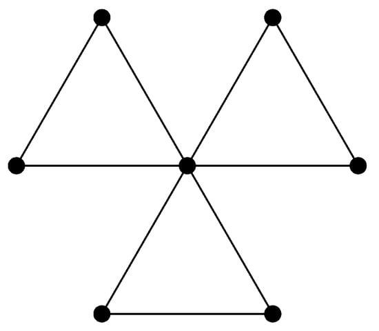
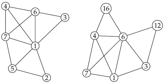
First, consider the graph shown in Figure 1.

Figure 1. Graph FyTAG in graph6 format.

Notice that the first three equations in (3) imply that this graph must be a subgraph of $\mathcal{G}$. We check with SageMath [28] that none of the following 29 graphs

$${\mathcal{G}}_1,{\mathcal{G}}_2,\dots ,{\mathcal{G}}_{19};{\mathcal{G}}_{25},{\mathcal{G}}_{26},\dots ,{\mathcal{G}}_{33};{\mathcal{G}}_{39}$$

has a subgraph isomorphic to the graph FyTAG. Hence, $\mathcal{G}$ is isomorphic to one of the graphs in the following set

$$\{{\mathcal{G}}_{20},{\mathcal{G}}_{21},{\mathcal{G}}_{22},{\mathcal{G}}_{23},{\mathcal{G}}_{24},{\mathcal{G}}_{34},{\mathcal{G}}_{35},{\mathcal{G}}_{36},{\mathcal{G}}_{37},{\mathcal{G}}_{38},{\mathcal{G}}_{40}\}.$$

(6)

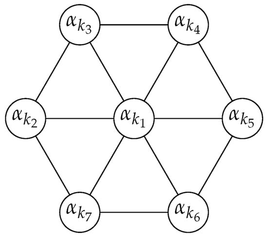
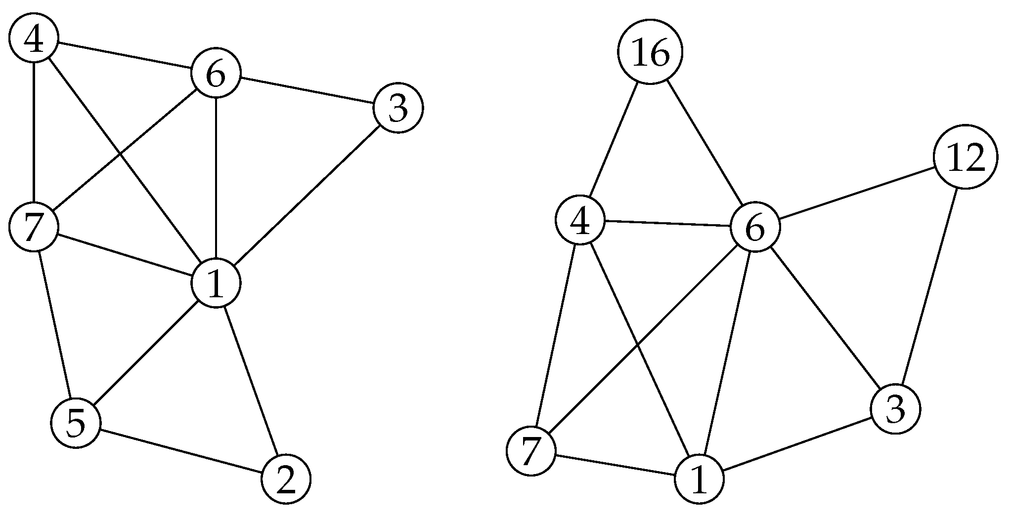
We claim that $\mathcal{G}$ is not isomorphic to any graph in the set $\{{\mathcal{G}}_{34},{\mathcal{G}}_{36},{\mathcal{G}}_{37},{\mathcal{G}}_{38}\}$. Indeed, consider the graph shown in Figure 2.

Figure 2. Graph F}TJG in graph6 format.

We will prove that this graph cannot be an induced subgraph of $\mathcal{G}$. Assume, to the contrary, that the graph F}TJG is an induced subgraph of $\mathcal{G}$. By $\left(ii\right)$ of Lemma 8, the edge $({\alpha }_{k_1},{\alpha }_{k_2})$ belongs to a zero-sum triangle $▵({\alpha }_{k_1},{\alpha }_{k_2},{\alpha }^{\prime })$, where ${\alpha }^{\prime }\in N\left({\alpha }_{k_1}\right)$. Since ${\alpha }_{k_3}$ and ${\alpha }_{k_7}$ are the only vertices in $N\left({\alpha }_{k_1}\right)$ that are adjacent to ${\alpha }_{k_2}$, we obtain that ${\alpha }^{\prime }={\alpha }_{k_3}$ or ${\alpha }_{k_7}$. Without loss of generality, assume ${\alpha }^{\prime }={\alpha }_{k_3}$. Thus, $▵({\alpha }_{k_1},{\alpha }_{k_2},{\alpha }_{k_3})$ is a zero-sum triangle. Now part $\left(i\right)$ of Lemma 8 implies that neither $▵({\alpha }_{k_1},{\alpha }_{k_3},{\alpha }_{k_4})$ nor $▵({\alpha }_{k_1},{\alpha }_{k_2},{\alpha }_{k_7})$ is a zero-sum triangle. Applying $\left(ii\right)$ of Lemma 8, we obtain that the edges $({\alpha }_{k_3},{\alpha }_{k_4})$ and $({\alpha }_{k_2},{\alpha }_{k_7})$ belong to zero-sum triangles $▵({\alpha }_{k_3},{\alpha }_{k_4},\tilde{\alpha })$ and $▵({\alpha }_{k_2},{\alpha }_{k_7},{\alpha }^{″})$, respectively, and $\tilde{\alpha },{\alpha }^{″}\notin N\left[{\alpha }_{k_1}\right]=\{{\alpha }_{k_1},{\alpha }_{k_2},\dots ,{\alpha }_{k_7}\}$.

Analogously, applying part $\left(ii\right)$ of Lemma 8, we obtain that

$$▵({\alpha }_{k_1},{\alpha }_{k_4},{\alpha }_{k_5})\mathrm{and}▵({\alpha }_{k_1},{\alpha }_{k_6},{\alpha }_{k_7})$$

are zero-sum triangles, $▵({\alpha }_{k_1},{\alpha }_{k_5},{\alpha }_{k_6})$ is not a zero-sum triangle and there exists a vertex ${\alpha }^{‴}$ such that $▵({\alpha }_{k_5},{\alpha }_{k_6},{\alpha }^{‴})$ is a zero-sum triangle and ${\alpha }^{‴}\notin N\left[{\alpha }_{k_1}\right]$.

Now, all obtained zero-sum triangles imply the relations

$$\begin{array}{c}{\alpha }_{k_1}+{\alpha }_{k_2}+{\alpha }_{k_3}=0,\hfill \\ {\alpha }_{k_1}+{\alpha }_{k_4}+{\alpha }_{k_5}=0,\hfill \\ {\alpha }_{k_1}+{\alpha }_{k_6}+{\alpha }_{k_7}=0,\hfill \\ {\alpha }_{k_3}+{\alpha }_{k_4}+\tilde{\alpha }=0,\hfill \\ {\alpha }_{k_5}+{\alpha }_{k_6}+{\alpha }^{\prime \prime \prime }=0,\hfill \\ {\alpha }_{k_2}+{\alpha }_{k_7}+{\alpha }^{\prime \prime }=0.\hfill \end{array}$$

(7)

By adding the first three relations in (7) and using the expressions for $\tilde{\alpha },{\alpha }^{″},$${\alpha }^{‴}$ from the last three relations in (7), we obtain

$$3{\alpha }_{k_1}+({\alpha }_{k_3}+{\alpha }_{k_4})+({\alpha }_{k_5}+{\alpha }_{k_6})+({\alpha }_{k_2}+{\alpha }_{k_7})=3{\alpha }_{k_1}-\tilde{\alpha }-{\alpha }^{‴}-{\alpha }^{″}=0.$$

If $\tilde{\alpha }={\alpha }^{″}={\alpha }^{‴}$, the last equality gives ${\alpha }_{k_1}=\tilde{\alpha }$, contrary to $\tilde{\alpha }\notin N\left[{\alpha }_{k_1}\right]$. Otherwise, collect equal terms among $\tilde{\alpha },{\alpha }^{″},{\alpha }^{‴}$, all of which differ from ${\alpha }_{k_1}$. The resulting relation has three or four distinct conjugates, with nonzero rational coefficients $(3,-2,-1)$ or $(3,-1,-1,-1)$, respectively. In both cases, the absolute value of the first coefficient equals the sum of the others’ absolute values, so Lemma 3 gives a contradiction.This proves that the graph F}TJG cannot be an induced subgraph of $\mathcal{G}$.

We check with SageMath [28] that each graph in $\{{\mathcal{G}}_{34},{\mathcal{G}}_{36},{\mathcal{G}}_{37},{\mathcal{G}}_{38}\}$ contains an induced subgraph isomorphic to F}TJG. Hence, $\mathcal{G}$ is not isomorphic to any of these graphs. This, together with (6), implies that $\mathcal{G}$ must be isomorphic to some graph in the following set

$$\{{\mathcal{G}}_{20},{\mathcal{G}}_{21},{\mathcal{G}}_{22},{\mathcal{G}}_{23},{\mathcal{G}}_{24},{\mathcal{G}}_{35},{\mathcal{G}}_{40}\}.$$

Next, we will prove that $\mathcal{G}$ is not isomorphic to any of the first five graphs in the set above, namely, $\{{\mathcal{G}}_{20},{\mathcal{G}}_{21},{\mathcal{G}}_{22},{\mathcal{G}}_{23},{\mathcal{G}}_{24}\}$.

The 16 vertices of each graph ${\mathcal{G}}_i$, $i\in \{20,21,22,23,24\}$, are labeled by the numbers $1,2,\dots ,16$. We will consider every such graph ${\mathcal{G}}_i$ separately. Assuming that $\mathcal{G}$ is isomorphic to ${\mathcal{G}}_i$, we will show that it leads to a contradiction. We will identify each vertex $v\in \{1,2,\dots ,16\}$ of ${\mathcal{G}}_i$ with ${\alpha }_v$. Thus, instead of treating $\mathcal{G}$ and ${\mathcal{G}}_i$ as isomorphic graphs, we will treat them as coinciding graphs, i.e., $\mathcal{G}={\mathcal{G}}_i$.

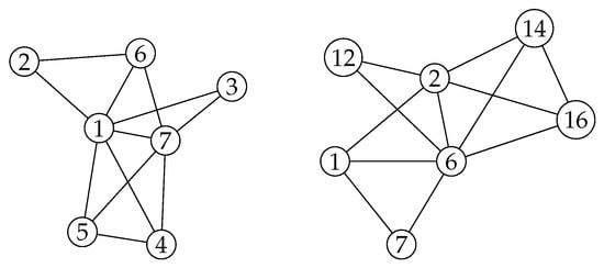
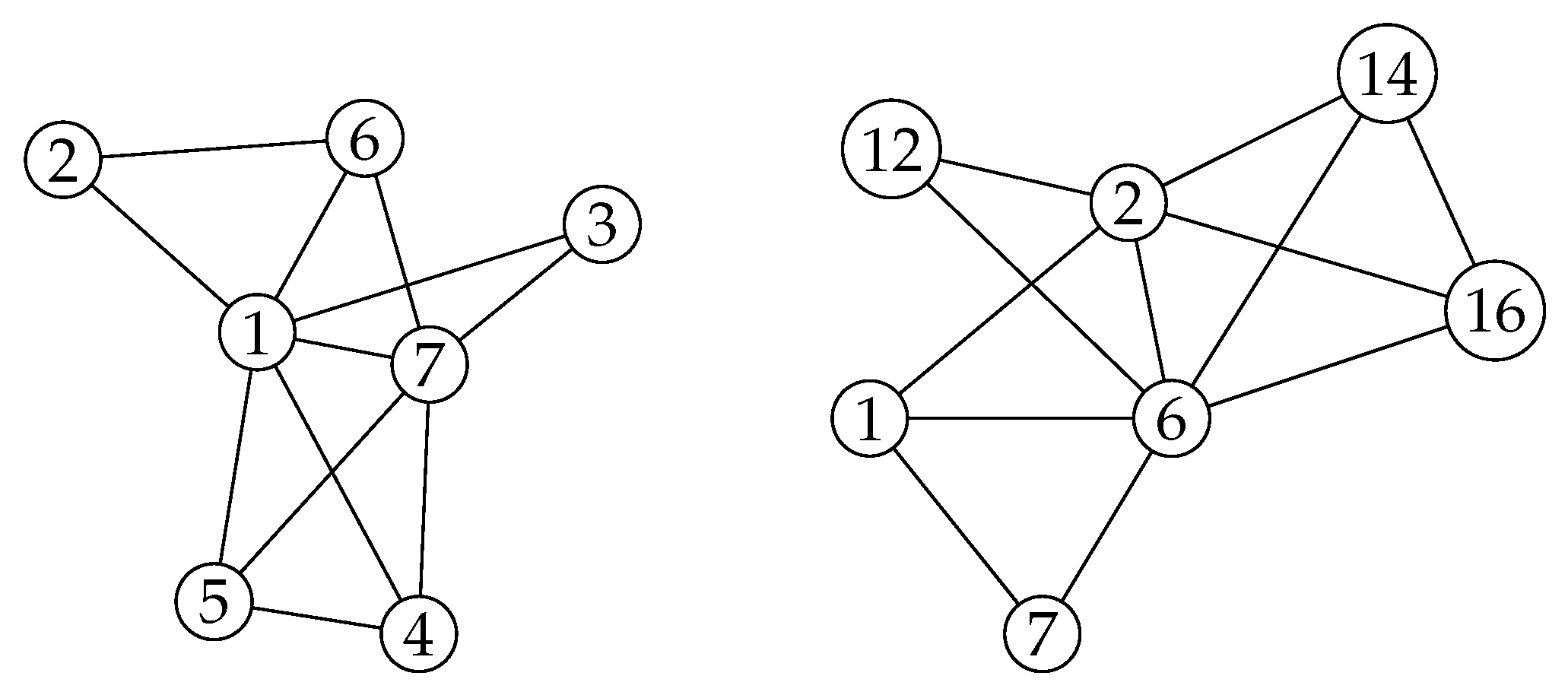
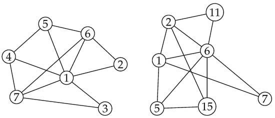
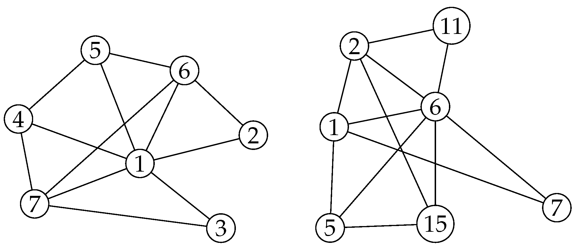
Assume that $\mathcal{G}={\mathcal{G}}_{20}$. The induced subgraphs ${\mathcal{G}}_{20}\left({\alpha }_1\right)$ and ${\mathcal{G}}_{20}\left({\alpha }_6\right)$ are shown in Figure 3.

Figure 3. Induced subgraphs ${\mathcal{G}}_{20}\left({\alpha }_1\right)$ and ${\mathcal{G}}_{20}\left({\alpha }_6\right)$.

We have that ${\alpha }_2,{\alpha }_6\in N\left({\alpha }_1\right)$, ${\mathrm{deg}}_{{\mathcal{G}}_{20}\left({\alpha }_1\right)}\left({\alpha }_2\right)=2$ and $({\alpha }_2,{\alpha }_6)$ is an edge in ${\mathcal{G}}_{20}$. Hence, part $\left(iii\right)$ of Lemma 8 implies that $▵({\alpha }_1,{\alpha }_2,$${\alpha }_6)$ is a zero-sum triangle. Similarly, ${\alpha }_1,{\alpha }_7\in N\left({\alpha }_6\right)$, ${\mathrm{deg}}_{{\mathcal{G}}_{20}\left({\alpha }_6\right)}\left({\alpha }_7\right)=2$ and $({\alpha }_1,{\alpha }_7)$ is an edge in ${\mathcal{G}}_{20}$. Again, applying part $\left(iii\right)$ of Lemma 8, we obtain that $▵({\alpha }_1,{\alpha }_6,{\alpha }_7)$ is a zero-sum triangle. Thus, the zero-sum triangles $▵({\alpha }_1,{\alpha }_2,{\alpha }_6)$ and $▵({\alpha }_1,{\alpha }_6,{\alpha }_7)$ share two distinct vertices ${\alpha }_1$ and ${\alpha }_6$. This contradicts part $\left(i\right)$ of Lemma 8. Thus, $\mathcal{G}\ne {\mathcal{G}}_{20}$.

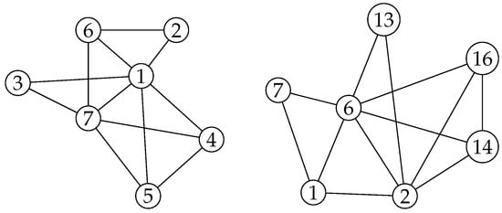
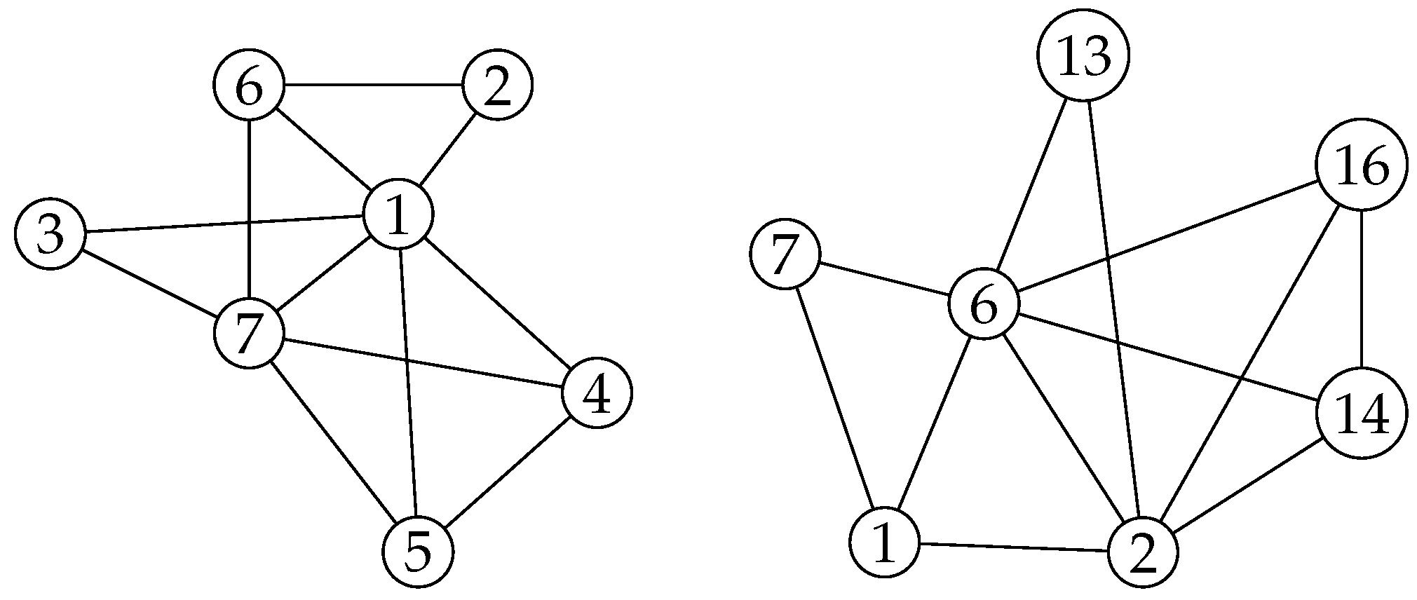
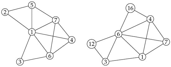
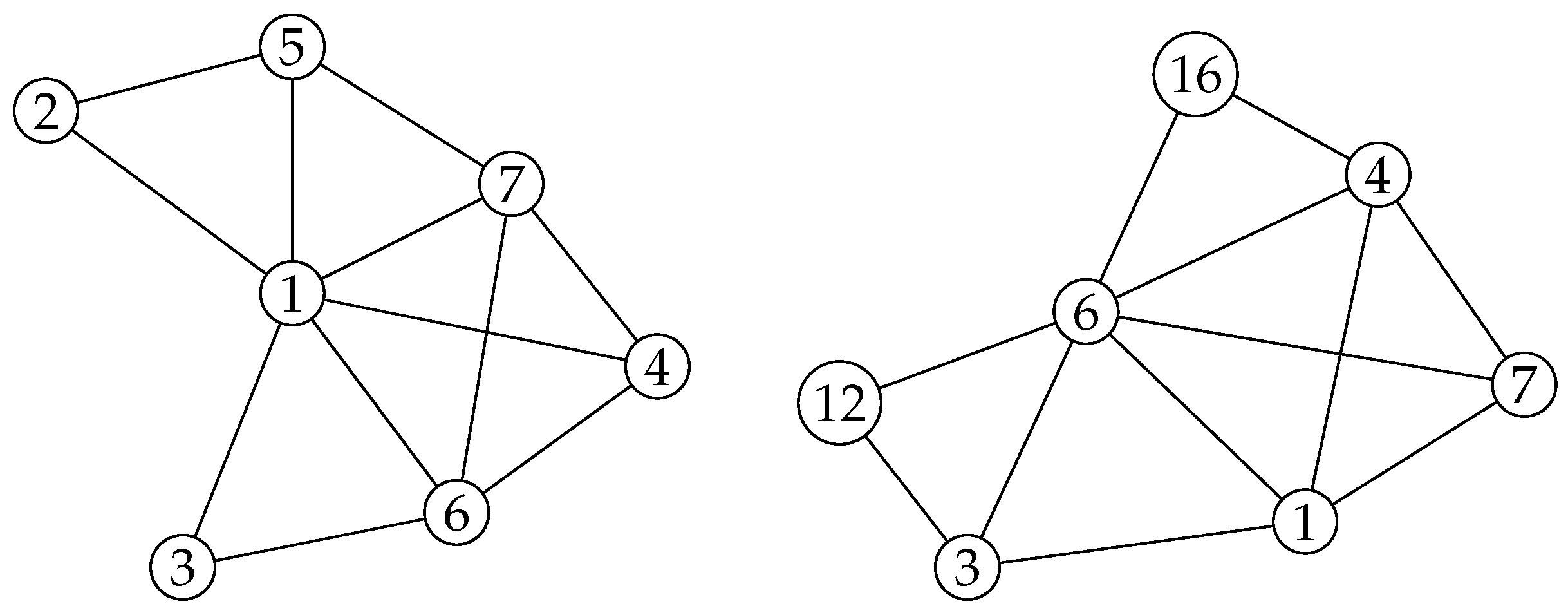
Table 2 gives the witnesses for all five cases, using the vertex labels in Figure 3, Figure 4, Figure 5, Figure 6 and Figure 7. Each ordered triple $(v,u,w)$ means that u has degree 2 in ${\mathcal{G}}_i\left(v\right)$ and is adjacent there to v and w. Lemma 8 (iii) therefore forces the corresponding zero-sum triangle. In every row, the two forced triangles share an edge, contradicting Lemma 8 (i).

Table 2. Forced zero-sum triangles; vertex numbers denote conjugates.

Graph Indices	$(\mathit{v},\mathit{u},\mathit{w})$, First	$(\mathit{v},\mathit{u},\mathit{w})$, Second	Shared Edge
$20,21,22$	$(1,2,6)$	$(6,7,1)$	$\{1,6\}$
$23,24$	$(1,3,6)$	$(6,12,3)$	$\{3,6\}$

Figure 4. Induced subgraphs ${\mathcal{G}}_{21}\left({\alpha }_1\right)$ and ${\mathcal{G}}_{21}\left({\alpha }_6\right)$.

Figure 5. Induced subgraphs ${\mathcal{G}}_{22}\left({\alpha }_1\right)$ and ${\mathcal{G}}_{22}\left({\alpha }_6\right)$.

Figure 6. Induced subgraphs ${\mathcal{G}}_{23}\left({\alpha }_1\right)$ and ${\mathcal{G}}_{23}\left({\alpha }_6\right)$.

Figure 7. Induced subgraphs ${\mathcal{G}}_{24}\left({\alpha }_1\right)$ and ${\mathcal{G}}_{24}\left({\alpha }_6\right)$.

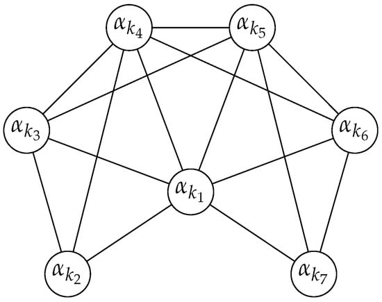
Hence, we are left with two cases: $\mathcal{G}={\mathcal{G}}_{35}$ or $\mathcal{G}={\mathcal{G}}_{40}$. To eliminate the first case, consider the graph shown in Figure 8.

Figure 8. Graph Fummw in graph6 format.

We will prove that this graph cannot be an induced subgraph of $\mathcal{G}$. Assume, to the contrary, that it is. By $\left(ii\right)$ of Lemma 8, the edge $({\alpha }_{k_1},{\alpha }_{k_2})$ belongs to a zero-sum triangle $▵({\alpha }_{k_1},{\alpha }_{k_2},{\alpha }^{\prime })$, where ${\alpha }^{\prime }\in N\left({\alpha }_{k_1}\right)$. Since ${\alpha }_{k_3}$ and ${\alpha }_{k_4}$ are the only vertices in $N\left({\alpha }_{k_1}\right)$ that are adjacent to ${\alpha }_{k_2}$, we obtain that ${\alpha }^{\prime }={\alpha }_{k_3}$ or ${\alpha }_{k_4}$. Thus, we have to consider two cases: $\left(i\right)$$▵({\alpha }_{k_1},{\alpha }_{k_2},{\alpha }_{k_3})$ is a zero-sum triangle; $\left(ii\right)$$▵({\alpha }_{k_1},{\alpha }_{k_2},{\alpha }_{k_4})$ is a zero-sum triangle.

Case $\left(i\right)$: $▵({\alpha }_{k_1},{\alpha }_{k_2},{\alpha }_{k_3})$ is a zero-sum triangle. By part $\left(ii\right)$ of Lemma 8, the edge $({\alpha }_{k_1},{\alpha }_{k_4})$ belongs to a zero-sum triangle $▵({\alpha }_{k_1},{\alpha }_{k_4},{\alpha }^{″})$, where ${\alpha }^{″}\in N\left({\alpha }_{k_1}\right)$. We have that ${\alpha }^{″}\in \{{\alpha }_{k_2},{\alpha }_{k_3},{\alpha }_{k_5},{\alpha }_{k_6}\}$, since ${\alpha }_{k_4}$ is not adjacent to ${\alpha }_{k_7}$. Part $\left(i\right)$ of Lemma 8 implies that neither $▵({\alpha }_{k_1},{\alpha }_{k_4},{\alpha }_{k_2})$ nor $▵({\alpha }_{k_1},{\alpha }_{k_4},$${\alpha }_{k_3})$ is a zero-sum triangle. Hence, ${\alpha }^{″}\in \{{\alpha }_{k_5},{\alpha }_{k_6}\}$.

Assume that ${\alpha }^{″}={\alpha }_{k_5}$. Then $▵({\alpha }_{k_1},{\alpha }_{k_4},{\alpha }_{k_5})$ and $▵({\alpha }_{k_1},{\alpha }_{k_2},{\alpha }_{k_3})$ are zero-sum triangles, while $({\alpha }_{k_2},{\alpha }_{k_4})$ and $({\alpha }_{k_3},{\alpha }_{k_5})$ are edges of $\mathcal{G}$. This contradicts part $\left(iv\right)$ of Lemma 8.

Assume that ${\alpha }^{″}={\alpha }_{k_6}$, so that $▵({\alpha }_{k_1},{\alpha }_{k_4},{\alpha }_{k_6})$ is a zero-sum triangle. Part $\left(i\right)$ of Lemma 8 implies that $▵({\alpha }_{k_1},{\alpha }_{k_6},{\alpha }_{k_7})$ is not a zero-sum triangle, since it shares an edge with the zero-sum triangle $▵({\alpha }_{k_1},{\alpha }_{k_4},{\alpha }_{k_6})$. Hence, $▵({\alpha }_{k_1},{\alpha }_{k_5},{\alpha }_{k_7})$ is a zero-sum triangle. Now, we have two zero-sum triangles $▵({\alpha }_{k_1},{\alpha }_{k_4},{\alpha }_{k_6})$ and $▵({\alpha }_{k_1},{\alpha }_{k_5},{\alpha }_{k_7})$, and $({\alpha }_{k_4},{\alpha }_{k_5})$ together with $({\alpha }_{k_6},{\alpha }_{k_7})$ are edges in $\mathcal{G}$. This contradicts part $\left(iv\right)$ of Lemma 8.

Case $\left(ii\right)$: $▵({\alpha }_{k_1},{\alpha }_{k_2},{\alpha }_{k_4})$ is a zero-sum triangle. Part $\left(i\right)$ of Lemma 8 implies that neither $▵({\alpha }_{k_1},{\alpha }_{k_3},{\alpha }_{k_2})$ nor $▵({\alpha }_{k_1},{\alpha }_{k_3},{\alpha }_{k_4})$ is a zero-sum triangle, since they share an edge with the zero-sum triangle $▵({\alpha }_{k_1},{\alpha }_{k_2},{\alpha }_{k_4})$. Hence, $▵({\alpha }_{k_1},{\alpha }_{k_3},{\alpha }_{k_5})$ is a zero-sum triangle. Now, we have two zero-sum triangles $▵({\alpha }_{k_1},{\alpha }_{k_2},{\alpha }_{k_4})$ and $▵({\alpha }_{k_1},{\alpha }_{k_3},{\alpha }_{k_5})$, and $({\alpha }_{k_2},{\alpha }_{k_3})$ together with $({\alpha }_{k_4},{\alpha }_{k_5})$ are edges in $\mathcal{G}$. This contradicts part $\left(iv\right)$ of Lemma 8.

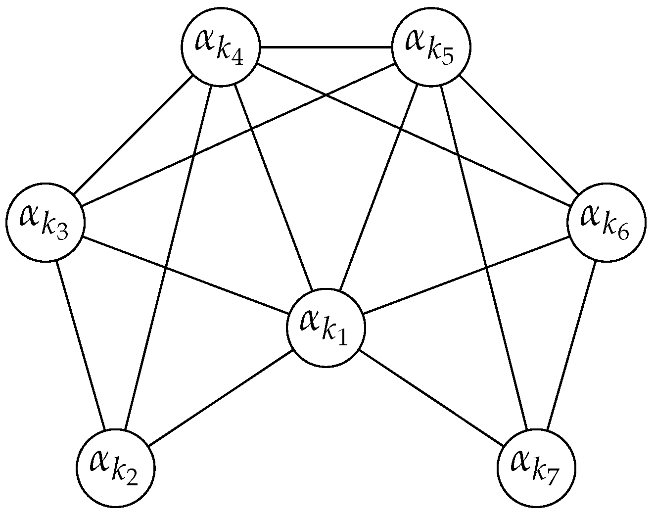
This completes the proof that the graph Fummw cannot be an induced subgraph of $\mathcal{G}$. We check with SageMath [28] that the graph ${\mathcal{G}}_{35}$ contains an induced subgraph isomorphic to Fummw. Therefore, $\mathcal{G}\ne {\mathcal{G}}_{35}$, and we are left to consider the last option $\mathcal{G}={\mathcal{G}}_{40}$. To do so, consider the graph shown in Figure 9.

Figure 9. Graph G~z\z{ in graph6 format.

We will prove that this graph cannot be an induced subgraph of $\mathcal{G}$. Assume, to the contrary, that it is. Part $\left(iii\right)$ of Lemma 7 implies that there exist three distinct relations ${\alpha }_{k_1}+{\alpha }_i^{\prime }+{\alpha }_i^{″}=0$, $i\in \{1,2,3\}$, which correspond to three distinct zero-sum triangles $▵({\alpha }_{k_1},{\alpha }_i^{\prime },{\alpha }_i^{″})$. Then part $\left(ii\right)$ of Lemma 8 yields ${\alpha }_i^{\prime },{\alpha }_i^{″}\in N\left({\alpha }_{k_1}\right)$ for every $i\in \{1,2,3\}$. Moreover, applying part $\left(i\right)$ of Lemma 8, we obtain that any two of the three sets $\{{\alpha }_i^{\prime },{\alpha }_i^{″}\}$, $i\in \{1,2,3\}$, are disjoint. Hence,

$$\{{\alpha }_1^{\prime },{\alpha }_1^{″},{\alpha }_2^{\prime },{\alpha }_2^{″},{\alpha }_3^{\prime },{\alpha }_3^{″}\}=N\left({\alpha }_{k_1}\right)=\{{\alpha }_{k_2},{\alpha }_{k_3},{\alpha }_{k_4},{\alpha }_{k_5},{\alpha }_{k_6},{\alpha }_{k_7}\}.$$

Now, adding up the relations ${\alpha }_{k_1}+{\alpha }_i^{\prime }+{\alpha }_i^{″}=0$, $i\in \{1,2,3\}$, we obtain

$$3{\alpha }_{k_1}+{\alpha }_{k_2}+{\alpha }_{k_3}+{\alpha }_{k_4}+{\alpha }_{k_5}+{\alpha }_{k_6}+{\alpha }_{k_7}=0.$$

(8)

Analogously, considering the three relations ${\alpha }_{k_8}+{\tilde{\alpha }}_i^{\prime }+{\tilde{\alpha }}_i^{″}=0$, $i\in \{1,2,3\}$, we obtain

$$3{\alpha }_{k_8}+{\alpha }_{k_2}+{\alpha }_{k_3}+{\alpha }_{k_4}+{\alpha }_{k_5}+{\alpha }_{k_6}+{\alpha }_{k_7}=0.$$

This equality, together with (8), implies that ${\alpha }_{k_1}={\alpha }_{k_8}$, which is a contradiction. Hence, the graph G~z\z{ cannot be an induced subgraph of $\mathcal{G}$. We check with SageMath [28] that the graph ${\mathcal{G}}_{40}$ contains an induced subgraph isomorphic to G~z\z{. Therefore, $\mathcal{G}\ne {\mathcal{G}}_{40}$.

Finally, we have proved that $\mathcal{G}\ne {\mathcal{G}}_i$ for $i=1,2,\dots 40$. Thus, no algebraic number of degree $d=16$ satisfies the relation (2).

References

- Dubickas, A.; Smyth, C.; Stong, R. Polynomials with Three Distinct Zeros Summing to Zero: 11123. Am. Math. Mon. 2006, 113, 941–942. [Google Scholar] [CrossRef] [Scilit]
- Baronėnas, Ž.; Drungilas, P.; Jankauskas, J. No three algebraic conjugates of degree sixteen sum to zero. arXiv 2026, arXiv:2608.03583. [Google Scholar]
- Kurbatov, V.A. Galoissche Erweiterungen vom Primzahlgrad und ihre primitiven Elemente. Izv. Vyssh. Uchebn. Zaved. Mat. 1977, 176, 61–66. [Google Scholar]
- Baron, G.; Drmota, M.; Skałba, M. Polynomial relations between polynomial roots. J. Algebra 1995, 177, 827–846. [Google Scholar] [CrossRef] [Scilit]
- Dixon, J.D. Polynomials with nontrivial relations between their roots. Acta Arith. 1997, 82, 293–302. [Google Scholar] [CrossRef] [Scilit]
- Girstmair, K. Linear relations between roots of polynomials. Acta Arith. 1999, 89, 53–96. [Google Scholar] [CrossRef] [Scilit]
- Girstmair, K. Linear dependence of zeros of polynomials and construction of primitive elements. Manuscr. Math. 1982, 39, 81–97. [Google Scholar] [CrossRef] [Scilit]
- Girstmair, K. The Galois relation x1 = x2 + x3 and Fermat over finite fields. Acta Arith. 2006, 124, 357–370. [Google Scholar] [CrossRef] [Scilit]
- Girstmair, K. The Galois relation x1 = x2 + x3 for finite simple groups. Acta Arith. 2007, 127, 301–303. [Google Scholar] [CrossRef] [Scilit]
- Girstmair, K. The Galois relations x1 = x2 + x3 and x1 = x2x3 for certain solvable groups. Ann. Sci. Math. Québec 2008, 32, 171–174. [Google Scholar]
- Lalande, F. La relation linéaire a = b + c + ⋯ + t entre les racines d’un polynôme. J. Théorie Nr. Bordx. 2007, 19, 473–484. [Google Scholar] [CrossRef] [Scilit]
- Lalande, F. À propos de la relation galoisienne x1 = x2 + x3. J. Théorie Nr. Bordx. 2010, 22, 661–673. [Google Scholar] [CrossRef] [Scilit]
- Dubickas, A.; Hare, K.G.; Jankauskas, J. No two non-real conjugates of a Pisot number have the same imaginary part. Math. Comput. 2017, 86, 935–950. [Google Scholar] [CrossRef] [Scilit]
- Dubickas, A.; Jankauskas, J. Simple linear relations between conjugate algebraic numbers of low degree. J. Ramanujan Math. Soc. 2015, 30, 219–235. [Google Scholar]
- Baronėnas, Ž.; Drungilas, P.; Jankauskas, J. Linear relations of four conjugates of an algebraic number. Can. Math. Bull. 2026, 69, 299–314. [Google Scholar] [CrossRef] [Scilit]
- Dubickas, A.; Virbalas, P. Additive and multiplicative relations with algebraic conjugates. Rev. Unión Mat. Argent. 2026, 69, 143–154. [Google Scholar] [CrossRef] [Scilit]
- Kitaoka, Y. Notes on the Distribution of Roots Modulo a Prime of a Polynomial. Unif. Distrib. Theory 2017, 12, 91–117. [Google Scholar] [CrossRef] [Scilit]
- Holgado, Á.S. Nontriviality of the module of relations for degree 4 polynomials. Acta Math. Hung. 2025, 176, 236–243. [Google Scholar] [CrossRef] [Scilit]
- Baronėnas, Ž.; Drungilas, P.; Jankauskas, J. No three algebraic conjugates of degree sixteen sum to zero. arXiv 2026, arXiv:2606.06222. [Google Scholar]
- McKay, B.D.; Royle, G.F. The transitive graphs with at most 26 vertices. Ars Comb. 1990, 30, 161–176. [Google Scholar]
- Royle, G.; Holt, D. Vertex-transitive Graphs On Fewer Than 48 Vertices. 2020. Available online: https://zenodo.org/records/4010122 (accessed on 21 August 2026).
- Smyth, C.J. Conjugate algebraic numbers on conics. Acta Arith. 1982, 40, 333–346. [Google Scholar] [CrossRef] [Scilit]
- Dubickas, A. On the degree of a linear form in conjugates of an algebraic number. Ill. J. Math. 2002, 46, 571–585. [Google Scholar] [CrossRef] [Scilit]
- Virbalas, P. Linear relations between three algebraic conjugates of degree twice a prime. Glas. Mat. 2025, 60, 229–242. [Google Scholar] [CrossRef] [Scilit]
- Coolsaet, K.; D’hondt, S.; Goedgebeur, J. House of Graphs 2.0: A database of interesting graphs and more. Discret. Appl. Math. 2023, 325, 97–107. [Google Scholar] [CrossRef] [Scilit]
- McKay, B.D.; Piperno, A. Practical graph isomorphism, II. J. Symb. Comput. 2014, 60, 94–112. [Google Scholar] [CrossRef] [Scilit]
- McKay, B.D. Description of graph6, sparse6 and digraph6 Encodings. Available online: https://users.cecs.anu.edu.au/~bdm/data/formats.txt (accessed on 30 May 2026).
- The Sage Developers. SageMath, the Sage Mathematics Software System (Version 10.6.0). 2025. Available online: https://www.sagemath.org (accessed on 24 August 2026).
Disclaimer/Publisher’s Note: The statements, opinions and data contained in all publications are solely those of the individual author(s) and contributor(s) and not of MDPI and/or the editor(s). MDPI and/or the editor(s) disclaim responsibility for any injury to people or property resulting from any ideas, methods, instructions or products referred to in the content. |
© 2026 by the authors. Licensee MDPI, Basel, Switzerland. This article is an open access article distributed under the terms and conditions of the Creative Commons Attribution (CC BY) license.