State-Space-Reconstructed High-Order Fully Actuated Control for Oxygen Excess Ratio Regulation in PEM Fuel Cells

Abstract

Precise oxygen excess ratio (OER) regulation in proton exchange membrane fuel cells must prevent oxygen starvation without excessive compressor power. Direct high-order fully actuated system (HOFAS) control differentiates an OER output whose actuation gain depends on stack current and becomes nonsmooth at ideal load steps. We instead control the supply-manifold-to-cathode pressure difference, yielding a second-order model with a constant nominal input coefficient, and use a third-order linear extended state observer (LESO) to estimate gain mismatch and nonlinear terms. A composite Lyapunov analysis establishes conditional uniform ultimate boundedness under smooth-load, bounded-disturbance-derivative, and unsaturated-input assumptions, with additional conditions for internal states and OER error. Simulations with parameter mismatch, measurement noise, actuator limits, sensing and actuation nonidealities, and a WLTC-like profile show bounded trajectories and a tracking–actuation trade-off. Output reconstruction reduces dependence on instantaneous current scheduling and supports rate-limited implementation, while direct-OER-HOFAS and super-twisting benchmarks can achieve lower tracking error at higher voltage activity.

1. Introduction

Proton exchange membrane fuel cells (PEMFCs) require cathode air management that supplies enough oxygen during load transients without excessive compressor power. The oxygen excess ratio (OER) is therefore a key regulated variable: low OER causes oxygen starvation, whereas excessive OER increases parasitic consumption [1,2]. Existing PI, disturbance-observer, sliding-mode, predictive, and prescribed-performance controllers improve robustness in different ways, but can require detailed models, online optimization, or high gains that amplify measurement noise and chattering [3,4,5,6,7,8,9,10,11,12,13].

The high-order fully actuated system (HOFAS) framework maps nonlinear dynamics to a parameterized linear closed-loop structure and has been combined with observers and predictive or sliding-mode controllers in several applications [14,15,16,17,18,19,20,21,22,23]. Its direct use with OER as the output, however, presents a structural limitation. Since ${\lambda }_{{\mathrm{O}}_2}=c_I(p_{\mathrm{sm}}-p_{\mathrm{ca}})$ with $c_I\propto I_{\mathrm{st}}^{-1}$, differentiating twice introduces load-dependent gain terms and derivatives of $c_I$. These derivatives are not classically bounded at an ideal current step, so the usual bounded-disturbance-derivative argument is not applicable there.

A particularly relevant recent direction is the nonlinear-observer-based HOFAS air-supply controller for fuel cells reported by Li et al. [23]. This fuel-cell-specific study is complemented by recent HOFAS observer developments based on extended-state observation [19] and high-gain derivative approximation for uncertain strict-feedback systems [21]; those studies establish useful estimation mechanisms but do not analyze the present PEMFC OER output-reconstruction issue. Li et al. demonstrate the value of combining HOFAS coordinates with nonlinear state/uncertainty estimation. The two designs address complementary sources of difficulty: a nonlinear observer can exploit plant nonlinearities in the estimation error injection, whereas the output reconstruction proposed here removes stack current from the multiplicative nominal input coefficient before observer tuning. The corresponding trade-off is that nonlinear-observer designs generally require more plant-specific model information and nonlinear-gain tuning, while the LESO used here has a transparent bandwidth parameterization. Consequently, replacing the LESO by a nonlinear observer would not, by itself, remove the $I_{\mathrm{st}}^{-1}$ dependence or the associated ${\dot{c}}_I$ and ${\ddot{c}}_I$ terms if OER remains the differentiated output. Conversely, output reconstruction does not claim that a linear observer is superior to the nonlinear observer in [23]; it isolates a structural regularity issue and gives a constant-$B_0$ analysis under explicitly stated conditions. Since the cited studies and the present work use different plant models, measured outputs, constraints, and test protocols, their numerical performance values should not be compared directly. A combined reconstructed-output/nonlinear-observer design is a natural next step, but it is outside the scope of this manuscript.

This study resolves that issue by reconstructing the controlled output as the pressure difference. The resulting nominal second-order model has an input coefficient independent of stack current; gain mismatch and nonlinear terms are estimated by a third-order linear extended state observer (LESO). A composite Lyapunov analysis states the precise smooth-load, bounded-disturbance-derivative, unsaturated-input, noise-free, and forward-completeness conditions for closed-loop UUB, while the disturbance-free case yields exponential tracking convergence. An internal-dynamics lemma and an OER-error corollary state the additional conditions needed to transfer these results to the physical states and OER.

The principal scientific contributions are:

(1)

A state-space-reconstructed HOFAS–LESO formulation that removes stack current from the nominal actuation gain.

(2)

A closed-loop architecture that combines adaptive pressure-difference reference generation, tracking differentiation, and LESO-based disturbance compensation.

(3)

A conditional stability analysis that gives the composite UUB result, its explicit ultimate-radius estimate, the disturbance-free exponential limit, and the stated internal-dynamics and OER-error corollaries.

Separately, the manuscript reports the following validation and reproducibility activities, which are not claimed as additional methodological contributions:

(4)

A controlled numerical comparison with PI, ISMC, relative-degree-consistent STSMC, HOFAS-without-LESO, and the strong gain-scheduled Direct-OER-HOFAS benchmark under common perturbation, noise, and actuator constraints.

(5)

Independent reproducibility and stress tests covering Monte Carlo noise realizations, time-step refinement, smooth-load assumption matching, sensing/actuation nonidealities, and a WLTC-like multisegment profile.

Items (4) and (5) document the scope, repeatability, and limitations of the proposed method rather than introducing new control-theoretic mechanisms.

2. Notation and Abbreviations

Table 1, Table 2 and Table 3 list, in numerical order, the principal variables, parameters, and abbreviations used in the model, controller, and numerical experiments. Units are SI units unless stated otherwise; “dimensionless” denotes a pure number. Symbols introduced only for intermediate proof steps are defined locally where they first occur.

Table 1. Symbols used in the PEMFC air-path and power model (Equations (1)–(15)).

Symbol	Meaning and SI Unit/Dimension
t	Time (s).
${\omega }_{\mathrm{cp}}$, $J_{\mathrm{cp}}$	Compressor angular speed (rad/s); compressor rotational inertia (kg m2).
${\tau }_{\mathrm{cm}}$, ${\tau }_{\mathrm{cp}}$	Motor electromagnetic torque and compressor load torque (N m).
$I_{\mathrm{cm}}$, $I_{\mathrm{st}}$	Compressor-motor armature current and stack current, respectively (A).
$v_{\mathrm{cm}}$	Applied compressor-motor voltage (V).
$R_{\mathrm{cm}}$, $k_v$, $k_t$, ${\eta }_{\mathrm{cm}}$	Armature resistance ($\mathsf{\Omega }$); back-EMF coefficient (V s/rad); motor torque constant (N m/A); motor efficiency (dimensionless).
$p_{\mathrm{sm}}$, $p_{\mathrm{ca}}$, $p_{\mathrm{atm}}$	Supply-manifold, cathode, and ambient pressures (Pa).
$V_{\mathrm{sm}}$, $V_{\mathrm{ca}}$	Supply-manifold and cathode volumes (m3).
$T_{\mathrm{sm}}$, $T_{\mathrm{ca}}$, $T_{\mathrm{atm}}$	Manifold, cathode, and ambient temperatures (K).
$W_{\mathrm{cp}}$, $W_{\mathrm{sm},\mathrm{out}}$, $W_{\mathrm{ca},\mathrm{out}}$	Compressor, manifold-outlet, and cathode-outlet mass flow rates (kg/s).
$W_{{\mathrm{O}}_2,\mathrm{rct}}$	Oxygen consumption rate in the electrochemical reaction (kg/s).
$c_1$, $c_2$	Linearized compressor-flow coefficients in $W_{\mathrm{cp}}=c_1{\omega }_{\mathrm{cp}}-c_2(p_{\mathrm{sm}}-p_{\mathrm{atm}})$ (kg/rad and kg/(s Pa)).
$k_{\mathrm{sm}}$, $k_{\mathrm{ca}}$	Manifold and cathode flow-restriction coefficients (kg/(s Pa)).
$R_a$, $C_p$, $\gamma$	Specific gas constant (J/(kg K)); specific heat capacity (J/(kg K)); heat-capacity ratio (dimensionless).
${\eta }_{\mathrm{cp}}$	Compressor isentropic efficiency (dimensionless).
$M_{{\mathrm{O}}_2}$, n, F	Oxygen molar mass (kg/mol); number of cells (dimensionless); Faraday constant (C/mol).
$x_{{\mathrm{O}}_2,\mathrm{atm}}$	Oxygen mass fraction in ambient air (dimensionless).
${\lambda }_{{\mathrm{O}}_2}$, ${\lambda }_{\mathrm{ref}}$, $c_I$	Oxygen excess ratio and reference (dimensionless); OER-to-pressure coefficient (Pa−1).
$V_{\mathrm{cell}}$, $E_{\mathrm{oc}}$, ${\eta }_{\mathrm{con}}$	Cell voltage, open-circuit voltage parameter, and concentration overpotential (V).
$P_{\mathrm{stack}}$, $P_{\mathrm{comp}}$, $P_{\mathrm{net}}$	Stack, compressor, and net power (W).

Table 2. Symbols used in the reconstructed HOFAS–LESO controller and analysis.

Symbol	Meaning and SI Unit/Dimension
y, $y_d$, $y_r$	Pressure difference $p_{\mathrm{sm}}-p_{\mathrm{ca}}$, raw reference, and tracking-differentiator reference (Pa).
u	Control input identified with $v_{\mathrm{cm}}$ (V).
$B_0$, $B_a$, $\Delta B$	Nominal, actual, and mismatch input coefficient (Pa/(s2 V)); units follow $\ddot{y}=\overline{f}+B_{0}u$.
$f_a$, $\overline{f}$, h	Actual drift, lumped drift including gain mismatch, and its derivative (Pa/s2, Pa/s3).
$y_1$, $y_2$, $y_3$	Extended-state coordinates $(y,\dot{y},\overline{f})$ with units Pa, Pa/s, and Pa/s2.
$z_1$, $z_2$, $z_3$	LESO state estimates with the same units as $y_1$, $y_2$, and $y_3$.
${\beta }_1$, ${\beta }_2$, ${\beta }_3$, ${\omega }_o$	LESO gains and observer bandwidth (s−1, s−2, s−3, and rad/s).
$k_1$, $k_2$, ${\omega }_c$	HOFAS/pole-placement gains and control bandwidth (s−1, s−2, and rad/s).
$r_{\mathrm{td}}$, ${\tau }_r$	Tracking-differentiator rate and measurement-filter time constant (rad/s and s).
${\widehat{\lambda }}_{{\mathrm{O}}_2}$, $\widehat{y}$, ${\widehat{I}}_{\mathrm{st}}$, ${\widehat{k}}_d$	Filtered OER, pressure difference, current, and adaptive reference gain (dimensionless, Pa, A, and Pa/A).
$e_o$, e, $e_{\lambda }$	Observer, pressure-tracking, and OER-tracking errors (Pa, Pa, and dimensionless).
$V_o$, $V_c$, $P_o$, $P_c$	Observer and closed-loop Lyapunov functions and their positive-definite matrices (energy-like scalars and matrices).
L, ${\delta }_r$, $\epsilon$	Bound on $\left|h\right|$, reference-generation mismatch, and small positive regularization constant (Pa/s3, Pa, and dimensionless or signal-unit dependent).
$\Delta t$, ${\dot{v}}_{\max }$	Numerical time step (s) and voltage slew-rate limit (V/s).
${\xi }_{\lambda }$, ${\xi }_y$	Unit Gaussian measurement-noise sequences (dimensionless).
IAE, ITAE	Integral absolute error and integral time-weighted absolute error (dimensionless-seconds and dimensionless-seconds2).
$\nu$, $s_{\mathrm{I}}$, $s_{\mathrm{ST}}$	STSMC integral state and ISMC/STSMC sliding variables (controller-scaled signal units).

Table 3. Abbreviations used in the manuscript.

Abbreviation	Expanded Form and Use
PEMFC	Proton exchange membrane fuel cell.
OER	Oxygen excess ratio.
HOFAS	High-order fully actuated system.
LESO/ESO	Linear extended state observer/extended state observer.
TD	Tracking differentiator.
PI	Proportional–integral controller.
ISMC	Integral sliding-mode control.
STSMC	Super-twisting sliding-mode control.
RL	Rate-limited implementation.
IAE/ITAE	Integral absolute error/integral time-weighted absolute error.
RK4	Classical fourth-order Runge–Kutta integration.
UUB	Uniform ultimate boundedness.
WLTC	Worldwide Harmonized Light Vehicles Test Cycle; here used only as a WLTC-like synthetic profile.

3. PEMFC Air-Supply Model and Problem Formulation

3.1. Control-Oriented Nonlinear Model

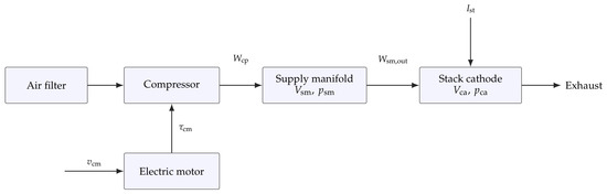
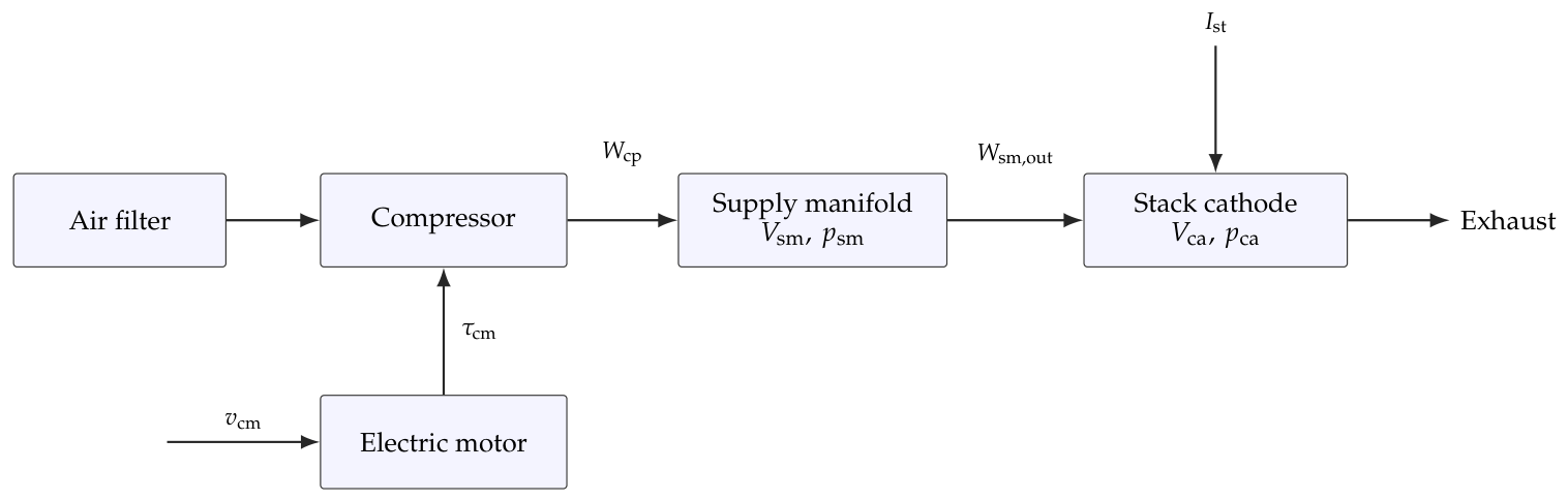
The cathode air path consists of an electric compressor, a supply manifold, and a stack cathode, as shown in Figure 1. A standard third-order control-oriented air-path model is adopted [1,2].

Figure 1. Control-oriented structure of the PEMFC cathode air-supply subsystem.

The compressor-shaft dynamics are

$${\dot{\omega }}_{\mathrm{cp}}={\displaystyle \frac{1}{J_{\mathrm{cp}}}}({\tau }_{\mathrm{cm}}-{\tau }_{\mathrm{cp}}),$$

(1)

where

$$I_{\mathrm{cm}}={\displaystyle \frac{v_{\mathrm{cm}}-k_v{\omega }_{\mathrm{cp}}}{R_{\mathrm{cm}}}},{\tau }_{\mathrm{cm}}={\eta }_{\mathrm{cm}}{k}_t{I}_{\mathrm{cm}}$$

(2)

and

$${\tau }_{\mathrm{cp}}={\displaystyle \frac{C_p{T}_{\mathrm{atm}}}{{\omega }_{\mathrm{cp}}{\eta }_{\mathrm{cp}}}}\left[{\left({\displaystyle \frac{p_{\mathrm{sm}}}{p_{\mathrm{atm}}}}\right)}^{(\gamma -1)/\gamma }-1\right]W_{\mathrm{cp}}.$$

(3)

The compressor mass flow is approximated in the operating region by

$$W_{\mathrm{cp}}=c_1{\omega }_{\mathrm{cp}}-c_2(p_{\mathrm{sm}}-p_{\mathrm{atm}}).$$

(4)

The supply-manifold and cathode pressures satisfy

$${\dot{p}}_{\mathrm{sm}}={\displaystyle \frac{R_a{T}_{\mathrm{sm}}}{V_{\mathrm{sm}}}}(W_{\mathrm{cp}}-W_{\mathrm{sm},\mathrm{out}}),$$

(5)

$${\dot{p}}_{\mathrm{ca}}={\displaystyle \frac{R_a{T}_{\mathrm{ca}}}{V_{\mathrm{ca}}}}(W_{\mathrm{sm},\mathrm{out}}-W_{\mathrm{ca},\mathrm{out}}-W_{{\mathrm{O}}_2,\mathrm{rct}}),$$

(6)

with

$$W_{\mathrm{sm},\mathrm{out}}=k_{\mathrm{sm}}(p_{\mathrm{sm}}-p_{\mathrm{ca}}),$$

(7)

$$W_{\mathrm{ca},\mathrm{out}}=k_{\mathrm{ca}}(p_{\mathrm{ca}}-p_{\mathrm{atm}}),$$

(8)

$$W_{{\mathrm{O}}_2,\mathrm{rct}}=M_{{\mathrm{O}}_2}{\displaystyle \frac{n{I}_{\mathrm{st}}}{4F}}.$$

(9)

$${\lambda }_{{\mathrm{O}}_2}={\displaystyle \frac{x_{{\mathrm{O}}_2,\mathrm{atm}}{W}_{\mathrm{sm},\mathrm{out}}}{W_{{\mathrm{O}}_2,\mathrm{rct}}}}=c_I(p_{\mathrm{sm}}-p_{\mathrm{ca}}),c_I={\displaystyle \frac{x_{{\mathrm{O}}_2,\mathrm{atm}}{k}_{\mathrm{sm}}}{W_{{\mathrm{O}}_2,\mathrm{rct}}}},$$

(10)

where $x_{{\mathrm{O}}_2,\mathrm{atm}}=0.233$.

For efficiency evaluation, the semi-empirical cell-voltage and power models are

$$V_{\mathrm{cell}}=E_{\mathrm{oc}}-0.0006I_{\mathrm{st}}-0.03\ln (I_{\mathrm{st}}+1)-{\eta }_{\mathrm{con}},$$

(11)

$${\eta }_{\mathrm{con}}=0.05{\left({\displaystyle \frac{{\lambda }_{\mathrm{ref}}}{{\lambda }_{{\mathrm{O}}_2}}}\right)}^4,{\lambda }_{\mathrm{ref}}=2,$$

(12)

$$P_{\mathrm{stack}}=n{V}_{\mathrm{cell}}{I}_{\mathrm{st}},$$

(13)

$$P_{\mathrm{comp}}=v_{\mathrm{cm}}\max (0,I_{\mathrm{cm}}),$$

(14)

$$P_{\mathrm{net}}=P_{\mathrm{stack}}-P_{\mathrm{comp}}.$$

(15)

The authors do not claim Equations (1)–(10) as original. The compressor-shaft balance, motor torque relation, compressor-flow approximation, manifold/cathode mass balances, restriction laws, and Faraday-law oxygen-consumption term in Equations (1)–(9) are adapted from the established control-oriented PEMFC air-path model of Pukrushpan et al. [1,2]. Equation (10) is the corresponding supplied-to-consumed oxygen-flow definition, also standard in that literature. The numerical constants and the compact cell-voltage/concentration-loss relations in Equations (11)–(15) are semi-empirical evaluation relations assembled for this study; their modeling role is stated explicitly, and they are not presented as a new electrochemical model. Their use is consistent with established PEMFC performance-modeling practice [24,25].

The signed armature current in Equation (2) permits active electrical braking and preserves the affine voltage channel used below. Negative braking energy is assumed to be dissipated by the drive and is not credited to net stack power, which explains the positive-part convention in $P_{\mathrm{comp}}$. Electrical-equivalent dynamic models provide a complementary route for stack-level model validation [25]. The present study instead retains the gas-path pressure and compressor dynamics because the manipulated voltage acts on the OER through the cathode air-supply subsystem.

Constant manifold temperatures and linearized flow restrictions are used, as is customary in control-oriented PEMFC studies. Their residual modeling errors are treated as part of the total disturbance.

3.2. Structural Limitation of Direct OER-Based HOFAS Control

If ${\lambda }_{{\mathrm{O}}_2}$ is directly selected as the HOFAS output, differentiating Equation (10) twice produces ${\dot{c}}_I$ and ${\ddot{c}}_I$. Moreover, the actuation coefficient has the form $B_{\lambda }=c_I{B}_0$ and thus changes with $I_{\mathrm{st}}$. An ideal load step makes the derivatives of $c_I$ distributional rather than classically bounded, and the load-dependent gain weakens direct pole-parameterization arguments.

The proposed reconstruction instead selects the pressure difference. Table 4 summarizes the distinction. The transformation does not claim that every disturbance derivative remains bounded at an ideal step; it removes load current from the multiplicative nominal gain and permits a rigorous analysis for smooth loads.

Table 4. Structural comparison of direct OER and reconstructed pressure-difference formulations.

Item	Direct OER Output	Reconstructed Output
Controlled output	${\lambda }_{{\mathrm{O}}_2}$	$p_{\mathrm{sm}}-p_{\mathrm{ca}}$
Fully actuated model	${\ddot{\lambda }}_{{\mathrm{O}}_2}=f_{\lambda }+B_{\lambda }u$	$\ddot{y}=\overline{f}+B_{0}u$
Nominal gain	$B_{\lambda }=c_I{B}_0$, $c_I\propto I_{\mathrm{st}}^{-1}$	Constant $B_0$
Load-current path	Gain and disturbance channels	Reference and additive disturbance channels
Step-load derivatives	Includes ${\dot{c}}_I,{\ddot{c}}_I$	Absent from nominal gain
Analysis condition	Time-varying gain must be handled	Constant nominal gain and bounded $\dot{\overline{f}}$

The table is read row by row. In the direct-OER formulation, the factor $c_I\propto I_{\mathrm{st}}^{-1}$ appears in the nominal input gain $B_{\lambda }=c_I{B}_0$ and in the differentiated disturbance channels; consequently, a load step changes the gain and introduces the nonclassical terms ${\dot{c}}_I$ and ${\ddot{c}}_I$. In the reconstructed formulation, the controlled variable is the pressure difference, so the nominal gain is the constant $B_0$; the stack current enters through the reference-generation path and the additive disturbance instead. Thus, the table summarizes a structural distinction in the two models. It does not assert that every disturbance derivative is bounded during an ideal step; the rigorous bounded-derivative analysis is restricted to the smooth-load conditions stated in Assumption 1.

4. State-Space-Reconstructed HOFAS-LESO Control

4.1. Output Reconstruction and Fully Actuated Transformation

The general HOFAS parameterization and pole-placement notation used in Equations (16)–(35) follow the HOFAS framework and observer/controller constructions reported by Duan and subsequent HOFAS studies [14,15,16,17,18,19,20,21,22,23]. The reconstructed-output formulation, algebraic reconstruction, adaptive reference path, and composite Lyapunov derivations that follow are the present paper’s formulation and analysis. The LESO structure itself is a standard active-disturbance-rejection observer, for which the cited observer references are provided [26,27,28,29,30]; the novelty claimed here is its integration with the reconstructed PEMFC pressure-difference model, not the observer equations in isolation.

$$y=p_{\mathrm{sm}}-p_{\mathrm{ca}}.$$

(16)

The OER is then related algebraically to the reconstructed output:

$${\lambda }_{{\mathrm{O}}_2}=c_{I}y.$$

(17)

For a target ${\lambda }_{{\mathrm{O}}_2}^{\ast }$, the nominal pressure-difference reference is

$$y_d={\displaystyle \frac{{\lambda }_{{\mathrm{O}}_2}^{\ast }}{c_I}}={\displaystyle \frac{{\lambda }_{{\mathrm{O}}_2}^{\ast }{M}_{{\mathrm{O}}_2}n}{4F{x}_{{\mathrm{O}}_2,\mathrm{atm}}{k}_{\mathrm{sm}}}}{I}_{\mathrm{st}}=k_d{I}_{\mathrm{st}}.$$

(18)

Using Equations (5) and (6),

$$\dot{y}={\displaystyle \frac{R_a{T}_{\mathrm{sm}}}{V_{\mathrm{sm}}}}(W_{\mathrm{cp}}-W_{\mathrm{sm},\mathrm{out}})-{\displaystyle \frac{R_a{T}_{\mathrm{ca}}}{V_{\mathrm{ca}}}}(W_{\mathrm{sm},\mathrm{out}}-W_{\mathrm{ca},\mathrm{out}}-W_{{\mathrm{O}}_2,\mathrm{rct}})$$

(19)

$$={\displaystyle \frac{R_a{T}_{\mathrm{sm}}}{V_{\mathrm{sm}}}}{c}_1{\omega }_{\mathrm{cp}}+f_1(p_{\mathrm{sm}},p_{\mathrm{ca}},I_{\mathrm{st}}),$$

(20)

where

$$\begin{array}{cc}\hfill f_1=& -{\displaystyle \frac{R_a{T}_{\mathrm{sm}}}{V_{\mathrm{sm}}}}\left[c_2(p_{\mathrm{sm}}-p_{\mathrm{atm}})+W_{\mathrm{sm},\mathrm{out}}\right]\hfill \\ \hfill & -{\displaystyle \frac{R_a{T}_{\mathrm{ca}}}{V_{\mathrm{ca}}}}(W_{\mathrm{sm},\mathrm{out}}-W_{\mathrm{ca},\mathrm{out}}-W_{{\mathrm{O}}_2,\mathrm{rct}}).\hfill \end{array}$$

(21)

Differentiating once more and substituting Equations (1) and (2) gives the actual plant model:

$$\ddot{y}=f_a+B_{a}u,u=v_{\mathrm{cm}},$$

(22)

where

$$B_a={\displaystyle \frac{R_a{T}_{\mathrm{sm}}}{V_{\mathrm{sm}}}}{\displaystyle \frac{c_1{\eta }_{\mathrm{cm}}{k}_t}{J_{\mathrm{cp}}{R}_{\mathrm{cm}}}},$$

(23)

$$f_a=-{\displaystyle \frac{R_a{T}_{\mathrm{sm}}}{V_{\mathrm{sm}}}}{\displaystyle \frac{c_1}{J_{\mathrm{cp}}}}\left({\displaystyle \frac{{\eta }_{\mathrm{cm}}{k}_t{k}_v}{R_{\mathrm{cm}}}}{\omega }_{\mathrm{cp}}+{\tau }_{\mathrm{cp}}\right)+{\dot{f}}_1.$$

(24)

The mismatch model is

$$\Delta B=B_a-B_0,\overline{f}=f_a+\Delta Bu,\ddot{y}=\overline{f}+B_{0}u.$$

(25)

The nominal coefficient is independent of $I_{\mathrm{st}}$; actual parameter variations enter the LESO disturbance channel through $\Delta Bu$.

The term $\Delta Bu$ makes the LESO disturbance matched but not exogenous: when the parameter mismatch $\Delta B$ is constant, $h=\dot{\overline{f}}={\dot{f}}_a+\Delta B\dot{u}$. Consequently, the bounded-h condition in Assumption 1 is a closed-loop regularity hypothesis that includes the applied-input trajectory; it is not an independent disturbance bound that holds for arbitrary controller commands. This is why the theorem is stated conditionally for a forward-complete, unsaturated solution in the smooth operating region. If saturation, rate limiting, actuator dynamics, or discontinuous load changes are included in the plant model, the corresponding applied input and augmented disturbance must be redefined and a new bound on h established before invoking the theorem.

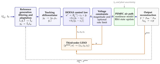
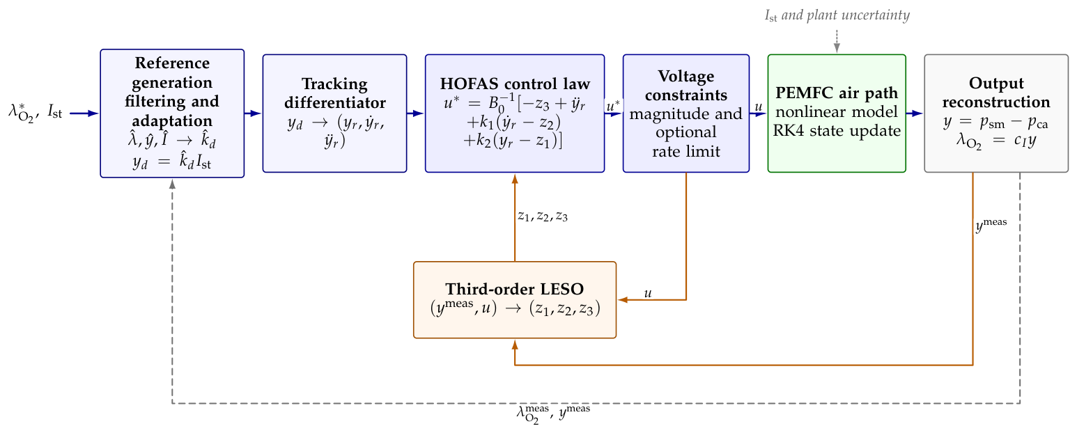
The complete reconstructed HOFAS–LESO architecture is shown in Figure 2.

Figure 2. Reconstructed HOFAS–LESO control architecture.

Remark 1.

At each sample, the measured OER ${\lambda }_{{\mathrm{O}}_2}^{\mathrm{meas}}$, pressure difference $y^{\mathrm{meas}}$, and stack current $I_{\mathrm{st}}$ first pass through the three filters with time constant ${\tau }_r$. Their states form the slowly varying coefficient ${\widehat{k}}_d$, while the unfiltered current provides the fast feedforward $y_d={\widehat{k}}_d{I}_{\mathrm{st}}$. The tracking differentiator supplies $(y_r,{\dot{y}}_r,{\ddot{y}}_r)$ to the HOFAS law. In parallel, the LESO receives the measured pressure difference and the applied voltage after magnitude and optional rate limiting, and returns $(z_1,z_2,z_3)$ for disturbance compensation. The constrained voltage drives the PEMFC air-path state update; the reconstructed pressure difference and OER then close the observer and reference-generation feedback paths.

4.2. Linear Extended State Observer

If $h\left(t\right)=\dot{\overline{f}}$ exists and is bounded, Equation (25) becomes

$${\dot{y}}_1=y_2,{\dot{y}}_2=y_3+B_{0}u,{\dot{y}}_3=h\left(t\right).$$

(26)

The third-order LESO is [26,27,28,29,30]

$$\begin{array}{cc}\hfill e_o& =z_1-y,\hfill \\ \hfill {\dot{z}}_1& =z_2-{\beta }_1{e}_o,\hfill \\ \hfill {\dot{z}}_2& =z_3+B_{0}u-{\beta }_2{e}_o,\hfill \\ \hfill {\dot{z}}_3& =-{\beta }_3{e}_o,\hfill \end{array}$$

(27)

with bandwidth parameterization

$${\beta }_1=3{\omega }_o,{\beta }_2=3{\omega }_o^2,{\beta }_3={\omega }_o^3.$$

(28)

4.3. Reference Generator and Control Law

The nominal reference in Equation (18) depends on $k_{\mathrm{sm}}$. To adapt the current-to-pressure coefficient while retaining fast load-current feedforward, filtered OER, pressure-difference, and stack-current signals are generated by the following filters:

$${\dot{\widehat{\lambda }}}_{{\mathrm{O}}_2}={\displaystyle \frac{{\lambda }_{{\mathrm{O}}_2}^{\mathrm{meas}}-{\widehat{\lambda }}_{{\mathrm{O}}_2}}{{\tau }_r}}.$$

(29)

$$\dot{\widehat{y}}={\displaystyle \frac{y^{\mathrm{meas}}-\widehat{y}}{{\tau }_r}}.$$

(30)

$${\dot{\widehat{I}}}_{\mathrm{st}}={\displaystyle \frac{I_{\mathrm{st}}-{\widehat{I}}_{\mathrm{st}}}{{\tau }_r}}.$$

(31)

The slowly calibrated coefficient and instantaneous reference are defined as follows:

$${\widehat{k}}_d={\displaystyle \frac{\widehat{y}}{\max ({\widehat{I}}_{\mathrm{st}},I_{\min })}}{\displaystyle \frac{{\lambda }_{{\mathrm{O}}_2}^{\ast }}{\max ({\widehat{\lambda }}_{{\mathrm{O}}_2},{ϵ}_r)}}.$$

(32)

$$y_d={\widehat{k}}_d{I}_{\mathrm{st}}.$$

(33)

Here $I_{\min }=10$ A and ${ϵ}_r=0.5$. The implementation uses ${\tau }_r=0.05$ s. At steady state, $I_{\mathrm{st}}={\widehat{I}}_{\mathrm{st}}$ and Equations (32) and (33) reduce to the algebraic OER-to-pressure relation; during a load transient, $I_{\mathrm{st}}/{\widehat{I}}_{\mathrm{st}}$ provides the explicitly modeled fast feedforward used in the simulations. A second-order tracking differentiator, represented in continuous time by

$${\ddot{y}}_r+2r_{\mathrm{td}}{\dot{y}}_r+r_{\mathrm{td}}^2{y}_r=r_{\mathrm{td}}^2{y}_d,$$

(34)

smooths discontinuous commands before their derivatives enter the control law.

The pressure-tracking error and control law are defined as follows:

$$\begin{array}{cc}\hfill e& =y-y_r,\hfill \\ \hfill u& ={\displaystyle \frac{1}{B_0}}\left[-z_3+{\ddot{y}}_r+k_1({\dot{y}}_r-z_2)+k_2(y_r-z_1)\right].\hfill \end{array}$$

(35)

The gains are

$$k_1=2{\omega }_c,k_2={\omega }_c^2.$$

(36)

Using ${\tilde{e}}_i=z_i-y_i$ gives

$$\ddot{e}+k_1\dot{e}+k_{2}e=-{\tilde{e}}_3-k_1{\tilde{e}}_2-k_2{\tilde{e}}_1.$$

(37)

4.4. Bandwidth Tuning and Practical Initial Selection

The three bandwidth-like quantities are selected in a fixed order so that pole placement, disturbance estimation, and reference smoothing are not tuned to compensate for one another. First, the controller bandwidth ${\omega }_c$ is selected from the required pressure-difference transient and the available voltage activity. Because $k_1=2{\omega }_c$ and $k_2={\omega }_c^2$, the nominal tracking polynomial is ${(s+{\omega }_c)}^2$; hence $1/{\omega }_c$ is the nominal closed-loop time constant and approximately $5.8/{\omega }_c$ is the 2% settling-time scale of the critically damped reference model. The initial value ${\omega }_c=30$ rad/s gives a 33.3 ms time constant and a 0.193 s nominal settling scale, which is fast relative to the imposed load segments while remaining a conservative starting point for the voltage-constrained simulation. Increasing it to 40 rad/s is retained as a sensitivity case rather than treated as an automatically better setting.

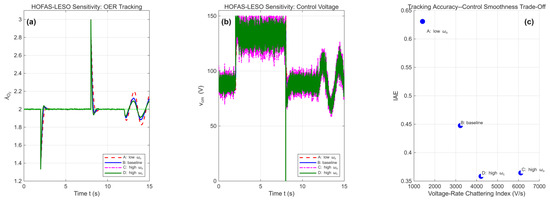
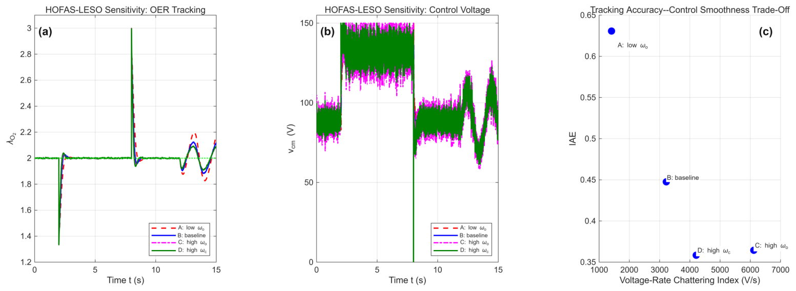
Second, the LESO bandwidth ${\omega }_o$ is selected after ${\omega }_c$ and is kept larger than the control bandwidth so that the lumped drift is estimated before it significantly affects the tracking error. The observer polynomial is ${(s+{\omega }_o)}^3$ from Equation (28), consistent with bandwidth parameterization practice [26,27]; the practical initial ratio ${\omega }_o/{\omega }_c=2.5$ therefore gives ${\omega }_o=75$ rad/s for ${\omega }_c=30$ rad/s. A smaller ratio leaves more observer lag, whereas a much larger ratio passes more measurement noise into $z_3$ and increases voltage activity. The reported sensitivity cases quantify this choice: ${\omega }_o=50$ raises IAE to 0.6307, while ${\omega }_o=100$ reduces IAE to 0.3644 but increases the voltage-rate index to 6114.04 V/s, compared with 3221.82 V/s at ${\omega }_o=75$.

Finally, the tracking-differentiator (observer-differentiator) bandwidth, denoted by $r_{\mathrm{td}}$ to distinguish it from the LESO bandwidth, is chosen to be at least as fast as the controller but close to the observer bandwidth. The filter in Equation (34) has polynomial ${(s+r_{\mathrm{td}})}^2$; $r_{\mathrm{td}}=80$ rad/s gives a nominal 2% smoothing time of approximately $5.8/r_{\mathrm{td}}=0.073$ s. This value is fast enough to pass the intended reference transitions, yet it regularizes the ideal step before ${\dot{y}}_r$ and ${\ddot{y}}_r$ enter the control law. The value is held fixed in the bandwidth-sensitivity table so that the effects of ${\omega }_o$ and ${\omega }_c$ remain identifiable.

$${\omega }_c^{\left(0\right)}=30\mathrm{rad}/\mathrm{s},{\omega }_o^{\left(0\right)}=2.5{\omega }_c^{\left(0\right)}=75\mathrm{rad}/\mathrm{s},r_{\mathrm{td}}^{\left(0\right)}=2.67{\omega }_c^{\left(0\right)}\approx 80\mathrm{rad}/\mathrm{s}.$$

(38)

For each candidate set, the same perturbed plant, initial equilibrium, load profile, sampling step, measurement realization, and voltage constraints are used. A candidate is retained only when the magnitude constraint is respected and the OER remains in the prescribed operating region; among feasible candidates, IAE is considered together with voltage-rate activity and net-power change. With the reported $\Delta t=1$ ms update, the fastest selected rates satisfy ${\omega }_o\Delta t=0.075$ and $r_{\mathrm{td}}\Delta t=0.080$, so the observer and differentiator dynamics are resolved without introducing a numerically stiff bandwidth. This procedure explains why $({\omega }_o,{\omega }_c,r_{\mathrm{td}})=(75,30,80)$ rad/s is used as the baseline: it is a reproducible compromise between observer lag, tracking speed, noise sensitivity, and actuator activity, not a claim of global parameter optimality. The measurement-filter time constant ${\tau }_r=0.05$ s is kept separate from these three bandwidths because it belongs to the adaptive reference calibration path rather than to the HOFAS error dynamics.

4.5. Uniform Ultimate Boundedness

Assumption 1

(Continuous-time analysis conditions).

1. 

$I_{\mathrm{st}}\in C^2$ satisfies $0<I_{\ast }\le I_{\mathrm{st}}\left(t\right)\le I^{\ast }<\infty$, and ${\dot{I}}_{\mathrm{st}}$ and ${\ddot{I}}_{\mathrm{st}}$ are bounded. The filtered current satisfies ${\widehat{I}}_{\mathrm{st}}\ge I_{\min }>0$, and the filters in Equations (29)–(31) and (34) produce bounded $y_r$, ${\dot{y}}_r$, and ${\ddot{y}}_r$.

2. 

$B_a=B_0+\Delta B$, and the lumped disturbance $\overline{f}=f_a+\Delta Bu$ is absolutely continuous with $\left|\dot{\overline{f}}\right|=\left|h\left(t\right)\right|\le L$ in the operating region. This is an imposed regularity condition; it is not a conclusion that u or $\dot{u}$ is globally bounded.

3. 

The ideal continuous-time control input is unsaturated, and the observer receives the noise-free output y.

4. 

The smoothed $y_r$ is treated as a bounded exogenous reference. The strict theorem conclusion concerns $y-y_r$; Corollary 2 relates this bound to OER tracking while retaining the reference-generation mismatch explicitly.

For the parameter-perturbation study, $J_{\mathrm{cp},\mathrm{a}}$ and $k_{\mathrm{sm},\mathrm{a}}$ are constant, so $\Delta B$ is constant and the input-dependent contribution to h is exactly $\Delta B\dot{u}$. If these coefficients vary with time, their variation contributes an additional term $\dot{\Delta B}u$ and must be included in the imposed bound on h.

Theorem 1

(Conditional UUB of the reconstructed closed loop). Under Assumption 1, consider Equations (25), (27) and (35). Let $k_1=2{\omega }_c$ and $k_2={\omega }_c^2$. If the composite Lyapunov weight ${\gamma }_o$ satisfies Equation (49), then the pressure-difference tracking errors $e=y-y_r$ and $\dot{e}$, together with the observer errors ${\tilde{e}}_i=z_i-y_i$, are uniformly ultimately bounded.

Proof. 

The observer-error dynamics are

$${\dot{\tilde{e}}}_1={\tilde{e}}_2-3{\omega }_o{\tilde{e}}_1,{\dot{\tilde{e}}}_2={\tilde{e}}_3-3{\omega }_o^2{\tilde{e}}_1,{\dot{\tilde{e}}}_3=-h\left(t\right)-{\omega }_o^3{\tilde{e}}_1.$$

(39)

Define ${ϵ}_i={\tilde{e}}_i/{\omega }_o^{i-1}$ and $\mathit{ϵ}={[{ϵ}_1,{ϵ}_2,{ϵ}_3]}^T$. Then

$$\dot{\mathit{ϵ}}={\omega }_o{A}_o\mathit{ϵ}+B_o{\displaystyle \frac{h\left(t\right)}{{\omega }_o^2}},A_o=\left[\begin{array}{ccc}-3& 1& 0\\ -3& 0& 1\\ -1& 0& 0\end{array}\right],B_o=\left[\begin{array}{c}0\\ 0\\ -1\end{array}\right].$$

(40)

$A_o$ is Hurwitz. Let $P_o>0$ solve $A_o^T{P}_o+P_o{A}_o=-I$ and set $V_o={\mathit{ϵ}}^T{P}_o\mathit{ϵ}$. Therefore,

$${\dot{V}}_o\le -{\omega }_o{\parallel \mathit{ϵ}\parallel }^2+{\displaystyle \frac{2\parallel P_o{B}_o\parallel L}{{\omega }_o^2}}\parallel \mathit{ϵ}\parallel .$$

(41)

Equation (41) gives the scaled-error order

$$\parallel \mathit{ϵ}\parallel =O\left({\displaystyle \frac{L}{{\omega }_o^3}}\right).$$

(42)

Returning to the unscaled coordinates gives

$$\left|{\tilde{e}}_1\right|=O\left({\displaystyle \frac{L}{{\omega }_o^3}}\right),\left|{\tilde{e}}_2\right|=O\left({\displaystyle \frac{L}{{\omega }_o^2}}\right),\left|{\tilde{e}}_3\right|=O\left({\displaystyle \frac{L}{{\omega }_o}}\right).$$

(43)

Thus, the $L/{\omega }_o^3$ order applies to the scaled error vector, not to every unscaled LESO state error.

Let $\mathit{\eta }={[e,\dot{e}]}^T$ and

$$A_c=\left[\begin{array}{cc}0& 1\\ -k_2& -k_1\end{array}\right],B_c=\left[\begin{array}{c}0\\ 1\end{array}\right].$$

(44)

Then $\dot{\mathit{\eta }}=A_c\mathit{\eta }-B_c({\tilde{e}}_3+k_1{\tilde{e}}_2+k_2{\tilde{e}}_1)$. Let $P_c>0$ solve $A_c^T{P}_c+P_c{A}_c=-I$, define $M_c=\parallel P_c{B}_c\parallel$, and consider

$$V={\mathit{\eta }}^T{P}_c\mathit{\eta }+{\gamma }_o{V}_o.$$

(45)

Using $\left|{\tilde{e}}_1\right|\le \parallel \mathit{ϵ}\parallel$, $\left|{\tilde{e}}_2\right|\le {\omega }_o\parallel \mathit{ϵ}\parallel$, $\left|{\tilde{e}}_3\right|\le {\omega }_o^2\parallel \mathit{ϵ}\parallel$, and Young’s inequality gives

$$\dot{V}\le -{\displaystyle \frac{1}{2}}{\parallel \mathit{\eta }\parallel }^2-a_o{\parallel \mathit{ϵ}\parallel }^2+d_o\parallel \mathit{ϵ}\parallel ,$$

(46)

$$a_o={\gamma }_o{\omega }_o-2M_c^2{({\omega }_o^2+2{\omega }_c{\omega }_o+{\omega }_c^2)}^2,$$

(47)

$$d_o={\displaystyle \frac{2{\gamma }_o\parallel P_o{B}_o\parallel L}{{\omega }_o^2}}.$$

(48)

Hence, $a_o>0$ if

$${\gamma }_o>{\displaystyle \frac{2M_c^2{({\omega }_o^2+2{\omega }_c{\omega }_o+{\omega }_c^2)}^2}{{\omega }_o}}.$$

(49)

Moreover, $-a_o{\parallel \mathit{ϵ}\parallel }^2+d_o\parallel \mathit{ϵ}\parallel \le -(a_o/2){\parallel \mathit{ϵ}\parallel }^2+d_o^2/\left(2a_o\right)$. Thus, $\dot{V}$ is negative outside a compact set, proving UUB of $\mathit{\eta }$ and $\mathit{ϵ}$, and therefore of e, $\dot{e}$, and ${\tilde{e}}_i$.

For ${\omega }_o=75$ and ${\omega }_c=30$, $P_c=\left[\begin{array}{cc}7.5417& 5.56\times {10}^{-4}\\ 5.56\times {10}^{-4}& 8.34\times {10}^{-3}\end{array}\right]$ and $M_c\approx 8.36\times {10}^{-3}$, so Equation (49) gives ${\gamma }_o>226.6$. This is sufficient, not necessary. With the generalized inequality $2ab\le \lambda a^2+b^2/\lambda$, $0<\lambda <1$, the bound becomes ${\gamma }_o>M_c^2{({\omega }_o^2+2{\omega }_c{\omega }_o+{\omega }_c^2)}^2/\left(\lambda {\omega }_o\right)$, illustrating the conservatism introduced by cross-term bounding. □

Corollary 1

(Closed-loop stability and tracking convergence). Under Assumption 1, consider a forward-complete ideal continuous-time solution in the stated operating region. Assume $B_0>0$, choose ${\omega }_o>0$ and ${\omega }_c>0$, and select ${\gamma }_o$ so that Equation (49) holds. Then the reconstructed closed-loop error state is uniformly ultimately bounded for every bounded disturbance derivative $\left|h\right(t\left)\right|\le L$. If $L=0$, the pressure-difference tracking error, its derivative, and all observer errors converge exponentially to zero. The OER error also converges to zero in this case provided the reference mismatch ${\delta }_r=y_r-y_d^{\ast }$ converges to zero.

Proof. 

The preceding Lyapunov calculation gives the explicit bound. Define

$$\mathit{\xi }={\left[\begin{array}{cc}{\mathit{\eta }}^T& {\mathit{ϵ}}^T\end{array}\right]}^T,Q=\mathrm{diag}(P_c,{\gamma }_o{P}_o),q_Q={\lambda }_{\max }\left(Q\right),c_Q=\min \left\{{\displaystyle \frac{1}{2}},{\displaystyle \frac{a_o}{2}}\right\}>0.$$

(50)

Since $V={\mathit{\xi }}^{T}Q\mathit{\xi }$, the estimate in Equation (46) and Young’s inequality imply

$$\dot{V}\le -c_Q{\parallel \mathit{\xi }\parallel }^2+{\displaystyle \frac{d_o^2}{2a_o}}\le -{\displaystyle \frac{c_Q}{q_Q}}V+{\displaystyle \frac{d_o^2}{2a_o}}.$$

(51)

Let ${\kappa }_Q=c_Q/q_Q>0$ and $b_Q=d_o^2/\left(2a_o\right)$. Applying the scalar comparison lemma to Equation (51) gives, for every $t\ge t_0$ along the forward-complete solution,

$$V\left(t\right)\le e^{-{\kappa }_Q(t-t_0)}V\left(t_0\right)+{\displaystyle \frac{b_Q}{{\kappa }_Q}}\left(1-e^{-{\kappa }_Q(t-t_0)}\right).$$

(52)

Therefore, for $L>0$ the complete reconstructed closed-loop error state is uniformly ultimately bounded, with

$$\underset{t\to \infty }{\lim \sup }V\left(t\right)\le {\overline{V}}_L:={\displaystyle \frac{q_Q{d}_o^2}{2a_o{c}_Q}},\underset{t\to \infty }{\lim \sup }\parallel \mathit{\eta }\left(t\right)\parallel \le \sqrt{{\displaystyle \frac{{\overline{V}}_L}{{\lambda }_{\min }\left(P_c\right)}}}.$$

(53)

In particular, this gives an explicit ultimate bound for the pressure-difference tracking error $\left|e\right|\le \parallel \mathit{\eta }\parallel$. If $L=0$ (equivalently, $h\left(t\right)\equiv 0$), then $d_o=0$ and Equation (51) reduces to $\dot{V}\le -(c_Q/q_Q)V$; hence, $\mathit{\eta }$ and $\mathit{ϵ}$ converge exponentially to zero, and so do e, $\dot{e}$, and all unscaled observer errors ${\tilde{e}}_i$. Thus, exact asymptotic pressure-difference tracking is guaranteed only in this disturbance-free ideal case; for bounded nonzero h, the rigorous guarantee is convergence to the stated UUB set. Exact OER tracking additionally requires the reference-generation mismatch ${\delta }_r=y_r-y_d^{\ast }$ to converge to zero; otherwise Corollary 2 gives the corresponding OER ultimate bound. □

Lemma 1

(Bounded internal dynamics). Under Assumption 1 and Theorem 1, the central conclusion is conditional internal-state boundedness: any forward-complete solution with positive physical coefficients that remains in the smooth compressor-model operating region ${\omega }_{\mathrm{cp}}>0$ has bounded $p_{\mathrm{ca}}$, $p_{\mathrm{sm}}$, and ${\omega }_{\mathrm{cp}}$.

Proof. 

Theorem 1 and bounded $y_r$ and ${\dot{y}}_r$ imply bounded $y=e+y_r$ and $\dot{y}=\dot{e}+{\dot{y}}_r$. Using $W_{\mathrm{sm},\mathrm{out}}=k_{\mathrm{sm}}y$ in Equation (6) gives

$${\dot{p}}_{\mathrm{ca}}=-a_{\mathrm{ca}}{p}_{\mathrm{ca}}+b_{\mathrm{ca}}\left(t\right),a_{\mathrm{ca}}={\displaystyle \frac{R_a{T}_{\mathrm{ca}}{k}_{\mathrm{ca}}}{V_{\mathrm{ca}}}}>0,$$

(54)

where

$$b_{\mathrm{ca}}\left(t\right)={\displaystyle \frac{R_a{T}_{\mathrm{ca}}}{V_{\mathrm{ca}}}}\left(k_{\mathrm{sm}}y+k_{\mathrm{ca}}{p}_{\mathrm{atm}}-{\displaystyle \frac{M_{{\mathrm{O}}_2}n{I}_{\mathrm{st}}}{4F}}\right).$$

(55)

Because y and $I_{\mathrm{st}}$ are bounded, $b_{\mathrm{ca}}$ is bounded; the exponentially stable scalar system (54) therefore gives bounded $p_{\mathrm{ca}}$. Equation (16) then gives bounded $p_{\mathrm{sm}}=p_{\mathrm{ca}}+y$. Finally, Equation (20) yields

$${\omega }_{\mathrm{cp}}={\displaystyle \frac{V_{\mathrm{sm}}}{R_a{T}_{\mathrm{sm}}{c}_1}}(\dot{y}-f_1).$$

(56)

The expression $f_1$ in Equation (21) is bounded when $p_{\mathrm{sm}}$, $p_{\mathrm{ca}}$, and $I_{\mathrm{st}}$ are bounded. The following estimates make the resulting bound on ${\omega }_{\mathrm{cp}}$ explicit.

Let $t_0$ be the initial time and define finite bounds $\overline{y}={\sup }_{t\ge t_0}\left|y\left(t\right)\right|$, $\overline{\dot{y}}={\sup }_{t\ge t_0}\left|\dot{y}\left(t\right)\right|$, and $\overline{I}=I^{\ast }$. Here, “uniformly ultimately bounded” is used in its standard sense: the trajectories are bounded for all $t\ge t_0$ and enter a fixed ultimate bound after a finite transient. Hence, Theorem 1 and the bounded reference in Assumption 1 imply $\overline{y},\overline{\dot{y}}<\infty$. Set ${\alpha }_{\mathrm{ca}}=R_a{T}_{\mathrm{ca}}/V_{\mathrm{ca}}$ and $q_{{\mathrm{O}}_2}=M_{{\mathrm{O}}_2}n/\left(4F\right)$. Then Equation (55) satisfies

$$|b_{\mathrm{ca}}\left(t\right)|\le {\overline{b}}_{\mathrm{ca}}:={\alpha }_{\mathrm{ca}}\left[k_{\mathrm{sm}}\overline{y}+k_{\mathrm{ca}}\left|p_{\mathrm{atm}}\right|+q_{{\mathrm{O}}_2}\overline{I}\right].$$

(57)

The variation-of-constants formula for Equation (54) therefore gives

$$\begin{array}{cc}\hfill |p_{\mathrm{ca}}\left(t\right)|& \le e^{-a_{\mathrm{ca}}(t-t_0)}\left|p_{\mathrm{ca}}\left(t_0\right)\right|+{\displaystyle \frac{{\overline{b}}_{\mathrm{ca}}}{a_{\mathrm{ca}}}}\left(1-e^{-a_{\mathrm{ca}}(t-t_0)}\right)\hfill \\ \hfill & \le {\overline{p}}_{\mathrm{ca}}:=\left|p_{\mathrm{ca}}\left(t_0\right)\right|+{\displaystyle \frac{{\overline{b}}_{\mathrm{ca}}}{a_{\mathrm{ca}}}}.\hfill \end{array}$$

(58)

Consequently, $|p_{\mathrm{sm}}\left(t\right)|\le {\overline{p}}_{\mathrm{sm}}:={\overline{p}}_{\mathrm{ca}}+\overline{y}$. Using $W_{\mathrm{sm},\mathrm{out}}=k_{\mathrm{sm}}y$ in Equation (21),

$$\begin{array}{cc}\hfill \left|f_1\left(t\right)\right|& \le {\overline{f}}_1:={\displaystyle \frac{R_a{T}_{\mathrm{sm}}}{V_{\mathrm{sm}}}}\left[c_2\left({\overline{p}}_{\mathrm{sm}}+\left|p_{\mathrm{atm}}\right|\right)+k_{\mathrm{sm}}\overline{y}\right]\hfill \\ \hfill & +{\alpha }_{\mathrm{ca}}\left[k_{\mathrm{sm}}\overline{y}+k_{\mathrm{ca}}\left({\overline{p}}_{\mathrm{ca}}+\left|p_{\mathrm{atm}}\right|\right)+q_{{\mathrm{O}}_2}\overline{I}\right].\hfill \end{array}$$

(59)

Since $R_a,T_{\mathrm{sm}},V_{\mathrm{sm}}$, and $c_1$ are positive, Equation (56) now yields the explicit speed bound

$$\left|{\omega }_{\mathrm{cp}}\left(t\right)\right|\le {\overline{\omega }}_{\mathrm{cp}}:={\displaystyle \frac{V_{\mathrm{sm}}}{R_a{T}_{\mathrm{sm}}{c}_1}}\left(\overline{\dot{y}}+{\overline{f}}_1\right)<\infty .$$

(60)

This estimate depends only on the bounded tracking/reference quantities, the initial cathode pressure, and the bounded stack current; it does not assume a bound on ${\omega }_{\mathrm{cp}}$ in order to establish the bound. □

Lemma 1 therefore emphasizes conditional, trajectory-wise boundedness of the internal pressure and compressor-speed states. It does not establish positive invariance of the sets $p_{\mathrm{sm}}>p_{\mathrm{atm}}$, $p_{\mathrm{ca}}\ge p_{\mathrm{atm}}$, and ${\omega }_{\mathrm{cp}}>0$ under the closed-loop vector field. The numerical implementation checks these domains at every integration step, but this check is not a proof of invariance or a global compressor-surge/physical-safety guarantee.

Corollary 2

(OER tracking bound). Let $y_d^{\ast }\left(t\right)={\lambda }_{{\mathrm{O}}_2}^{\ast }/c_I\left(t\right)$ denote the exact algebraic pressure-difference reference and ${\delta }_r=y_r-y_d^{\ast }$. If e and ${\delta }_r$ are uniformly ultimately bounded with respective ultimate bounds $\overline{e}$ and ${\overline{\delta }}_r$, so that

$$\underset{t\to \infty }{\lim \sup }\left|e\left(t\right)\right|\le \overline{e},\underset{t\to \infty }{\lim \sup }\left|{\delta }_r\left(t\right)\right|\le {\overline{\delta }}_r,$$

(61)

then the OER tracking error is uniformly ultimately bounded and satisfies

$$\underset{t\to \infty }{\lim \sup }|{\lambda }_{{\mathrm{O}}_2}\left(t\right)-{\lambda }_{{\mathrm{O}}_2}^{\ast }\left(t\right)|\le {\overline{c}}_I(\overline{e}+{\overline{\delta }}_r),{\overline{c}}_I={\displaystyle \frac{4F{x}_{{\mathrm{O}}_2,\mathrm{atm}}{k}_{\mathrm{sm}}}{M_{{\mathrm{O}}_2}n{I}_{\ast }}}.$$

(62)

Proof. 

Assumption 1 gives $I_{\mathrm{st}}\ge I_{\ast }>0$ and hence $0<c_I\left(t\right)\le {\overline{c}}_I$. Equation (17) and ${\lambda }_{{\mathrm{O}}_2}^{\ast }=c_I{y}_d^{\ast }$ give

$${\lambda }_{{\mathrm{O}}_2}-{\lambda }_{{\mathrm{O}}_2}^{\ast }=c_I(y-y_d^{\ast })=c_I(e+{\delta }_r).$$

(63)

Taking the limit superior and applying the triangle inequality proves Equation (62). □

Remark 2.

Theorem 1 does not cover ideal load steps, sensor noise, or input saturation. The assumption-matched check in Section 5 is the only numerical case intended to mirror the smooth-load, noise-free, unsaturated hypotheses; it checks consistency of the implementation but does not replace the proof or establish a data-driven bound on h. Lemma 1 establishes boundedness along a solution in the smooth compressor operating region but does not prove positive invariance of that region. Corollary 2 retains the reference-generation mismatch ${\delta }_r$ rather than assuming that the adaptive reference is exact. The ideal-step, noisy, saturated, rate-limited, delayed, biased, and lagged cases are deliberately retained as discrete-time engineering stress tests and are not presented as direct numerical verification of the continuous-time UUB result.

5. Numerical Results

5.1. Simulation Configuration

The nonlinear model is implemented in MWORKS using a fixed-step fourth-order Runge–Kutta scheme with $\Delta t=0.001$ s. The time vectors are generated as integer multiples of $\Delta t$, including both endpoints. Table 5 lists the nominal parameters.

Table 5. Nominal parameters of the PEMFC cathode air-supply model.

Parameter	Symbol	Value
Compressor inertia	$J_{\mathrm{cp}}$	$5\times {10}^{-5}$ kg m2
Cathode volume	$V_{\mathrm{ca}}$	$0.01$ m3
Supply-manifold volume	$V_{\mathrm{sm}}$	$0.02$ m3
Air gas constant	$R_a$	287 J/(kg K)
Manifold/cathode temperature	$T_{\mathrm{sm}},T_{\mathrm{ca}}$	353 K
Ambient temperature	$T_{\mathrm{atm}}$	298 K
Ambient pressure	$p_{\mathrm{atm}}$	$101,325$ Pa
Specific heat	$C_p$	1005 J/(kg K)
Heat-capacity ratio	$\gamma$	$1.4$
Compressor efficiency	${\eta }_{\mathrm{cp}}$	$0.8$
Motor efficiency	${\eta }_{\mathrm{cm}}$	$0.9$
Torque constant	$k_t$	$0.05$ N m/A
Stator resistance	$R_{\mathrm{cm}}$	$0.8\mathsf{\Omega }$
Back-EMF coefficient	$k_v$	$0.05$ V/(rad/s)
Compressor-flow coefficients	$c_1,c_2$	$2\times {10}^{-5},5\times {10}^{-7}$
Manifold restriction	$k_{\mathrm{sm}}$	$2\times {10}^{-6}$ kg/(s Pa)
Cathode restriction	$k_{\mathrm{ca}}$	$1.8\times {10}^{-6}$ kg/(s Pa)
Oxygen molar mass	$M_{{\mathrm{O}}_2}$	$0.032$ kg/mol
Faraday constant	F	$96,485$ C/mol
Atmospheric oxygen mass fraction	$x_{{\mathrm{O}}_2,\mathrm{atm}}$	$0.233$
Number of cells	n	300
Open-circuit voltage coefficient	$E_{\mathrm{oc}}$	$1.05$ V

The actual plant uses $J_{\mathrm{cp},\mathrm{a}}=1.2J_{\mathrm{cp}}$ and $k_{\mathrm{sm},\mathrm{a}}=0.8k_{\mathrm{sm}}$, while every controller retains nominal parameters. Independent unit Gaussian sequences ${\xi }_{\lambda }$ and ${\xi }_y$ are generated once with random seed 42 and shared by all controllers. The measured signals are ${\lambda }^{\mathrm{meas}}=\lambda (1+0.01{\xi }_{\lambda })$ and $y^{\mathrm{meas}}=y(1+0.01{\xi }_y)$, so the conditional standard deviation is exactly 1% of each instantaneous signal. All control voltages are limited to 0–150 V and initialized with their operating-point bias at 100 A.

The PI baseline uses $K_p=15$ and $K_i=60$ with integral anti-windup. For the two sliding-mode baselines, let $e_{\lambda }={\lambda }_{{\mathrm{O}}_2}^{\mathrm{meas}}-{\lambda }_{{\mathrm{O}}_2}^{\ast }$ and let ${\widehat{\dot{e}}}_{\lambda }$ denote an 80 rad/s low-pass derivative estimate. The ISMC implementation is

$$s_{\mathrm{I}}={\widehat{\dot{e}}}_{\lambda }+c_s{e}_{\lambda }+c_i\int e_{\lambda }dt,$$

(64)

$$v_{\mathrm{cm}}=v_{\mathrm{cm},0}+B_{\lambda }^{-1}\left[-c_s{\widehat{\dot{e}}}_{\lambda }-c_i{e}_{\lambda }-{\eta }_{\mathrm{smc}}\mathrm{sat}\left({\displaystyle \frac{s_{\mathrm{I}}}{\mathsf{\Phi }}}\right)-k_{\mathrm{smc}}{s}_{\mathrm{I}}\right],$$

(65)

with $c_s=20$, $c_i=15$, ${\eta }_{\mathrm{smc}}=15$, $k_{\mathrm{smc}}=20$, and $\mathsf{\Phi }=0.05$. Because the OER has a relative degree of two with respect to compressor voltage, the STSMC sliding variable includes the error derivative so that $s_{\mathrm{ST}}$ has a relative degree of one:

$$s_{\mathrm{ST}}={\widehat{\dot{e}}}_{\lambda }+c_{\mathrm{ST}}{e}_{\lambda },$$

(66)

$$\dot{\nu }=-{\alpha }_{\mathrm{ST}}{\sigma }_{{\mathsf{\Phi }}_{\mathrm{ST}}}\left(s_{\mathrm{ST}}\right),$$

(67)

$$v_{\mathrm{cm}}=v_{\mathrm{cm},0}+B_{\lambda }^{-1}\left[-c_{\mathrm{ST}}{\widehat{\dot{e}}}_{\lambda }-{\lambda }_{\mathrm{ST}}\sqrt{|s_{\mathrm{ST}}|+{ϵ}_s}{\sigma }_{{\mathsf{\Phi }}_{\mathrm{ST}}}\left(s_{\mathrm{ST}}\right)+\nu \right],$$

(68)

where ${\sigma }_{\mathsf{\Phi }}\left(s\right)=\mathrm{sign}\left(s\right)$ for $\left|s\right|>\mathsf{\Phi }$ and ${\sigma }_{\mathsf{\Phi }}\left(s\right)=s/\mathsf{\Phi }$ otherwise [31]. A finite, reproducible grid uses $c_{\mathrm{ST}}\in \{10,20,30,40,60\}$, ${\lambda }_{\mathrm{ST}}\in \{20,40,60,80,120\}$, ${\alpha }_{\mathrm{ST}}\in \{100,200,400,800,1600\}$, and ${\mathsf{\Phi }}_{\mathrm{ST}}\in \{0.1,0.25,0.5\}$. The minimum-IAE candidate satisfying the common 0–150 V constraint is $(60,120,1600,0.1)$; the normalized integral state is limited to $\left|\nu \right|\le 2000$ for anti-windup. HOFAS-NoESO uses the same adaptive reference, reconstructed output, ${\omega }_c=30$, $r_{\mathrm{td}}=80$ rad/s, and operating-point bias $v_{\mathrm{cm},0}$, but omits online disturbance estimation. HOFAS-LESO uses ${\omega }_o=75$, ${\omega }_c=30$, and $r_{\mathrm{td}}=80$ rad/s.

The baseline HOFAS–LESO values used in the numerical experiments are ${\omega }_o=75$, ${\omega }_c=30$, and $r_{\mathrm{td}}=80$ rad/s, as selected by the procedure in Section 4. These quantities are bandwidths, so all three are expressed in rad/s; the sensitivity cases below vary ${\omega }_o$ and ${\omega }_c$ while retaining $r_{\mathrm{td}}=80$ rad/s.

For a direct test of the output-selection argument, Direct-OER-HOFAS uses the measured OER as the LESO output and the exact nominal gain schedule

$$B_{\lambda }\left(I_{\mathrm{st}}\right)={\displaystyle \frac{x_{{\mathrm{O}}_2,\mathrm{atm}}{k}_{\mathrm{sm}}}{M_{{\mathrm{O}}_2}n{I}_{\mathrm{st}}/\left(4F\right)}}{B}_0.$$

(69)

Its observer and controller use the same ${\omega }_o=75$ and ${\omega }_c=30$ as the reconstructed method.

This benchmark is informative because it uses the instantaneous load current to invert $B_{\lambda }\left(I_{\mathrm{st}}\right)$ at every sample; it is not covered by the constant-gain proof in Section 4.

To assess actuator feasibility, HOFAS-LESO-RL applies the original command $v_k^{\ast }$ through

$$v_k^{\mathrm{RL}}=\mathrm{clip}\left(v_k^{\ast },v_{k-1}^{\mathrm{RL}}-{\dot{v}}_{\max }\Delta t,v_{k-1}^{\mathrm{RL}}+{\dot{v}}_{\max }\Delta t\right),{\dot{v}}_{\max }=1000\mathrm{V}/\mathrm{s},$$

(70)

followed by the common 0–150 V magnitude constraint. The LESO is updated with the applied, rather than unconstrained, voltage.

The 15 s stress-test profile starts at 100 A, steps to 150 A at 2 s, returns to 100 A at 8 s, and becomes $I_{\mathrm{st}}=100+20\sin \left(\pi (t-12)\right)$ A after 12 s. The ideal steps, multiplicative measurement noise, and 0–150 V magnitude constraint are deliberately retained to test the sampled implementation under engineering conditions. Only the sinusoidal segment satisfies the smooth-load assumption of Theorem 1; consequently, the results based on this profile are not presented as a direct numerical verification of that theorem.

5.2. Alignment of Theoretical Conditions and Numerical Cases

To make the relationship between the theorem and the simulations explicit, we include a separate assumption-matched check using the same perturbed plant and HOFAS–LESO controller. The stack current is $I_{\mathrm{st}}\left(t\right)=100+20\sin \left(\pi t\right)$ A over the complete 15 s interval, which is $C^{\infty }$ and satisfies $80\le I_{\mathrm{st}}\le 120$ A, $\left|{\dot{I}}_{\mathrm{st}}\right|\le 20\pi \mathrm{A}/\mathrm{s}$, and $\left|{\ddot{I}}_{\mathrm{st}}\right|\le 20{\pi }^2\mathrm{A}/{\mathrm{s}}^2$. The output measurements are noise free, measurement delay and sensor bias are disabled, and both the voltage-magnitude and voltage-rate limiters are disabled.

In this condition-matched run, the IAE is 1.112215.

The OER range is $[1.884471,2.122036]$.

The unconstrained commanded voltage remains in $[68.8947,108.0243]$ V (maximum sample-to-sample rate 499.06 V/s). Thus, the 0–150 V saturation is inactive in this run. The finite trajectory and bounded numerical input are reported as a consistency check for the stated operating conditions; they do not constitute an empirical proof of the analytical bound $\left|h\right(t\left)\right|\le L$, which remains an assumption of Theorem 1.

The primary comparison in Table 6, the Monte Carlo study, and the rate-limited, delayed, biased, and actuator-lag cases are therefore engineering stress tests. They intentionally violate one or more hypotheses of the theorem and are used to quantify performance degradation and implementation feasibility, not to claim UUB under noise, saturation, ideal steps, delays, biases, or unmodeled actuator dynamics. The noise-free time-step study removes measurement noise but retains the ideal steps and magnitude saturation, so it is a discretization check rather than the assumption-matched theorem check above.

Table 6. Performance under 20% parameter perturbation and multiplicative 1% measurement noise.

Controller	Min. OER	Max. OER	IAE	ITAE	Settling (s)	Mean ${\mathit{P}}_{\mathbf{net}}$ (kW)	Rate Index (V/s)	Max. Rate (V/s)
PI	1.3333	1.9964	2.0171	16.3545	2.1810	27.0972	433.71	14,831.88
ISMC	1.3331	1.8836	2.9302	22.0372	N/A	26.8741	6500.38	125,069.26
STSMC	1.3333	2.0115	0.3362	2.6058	0.2860	26.7279	23,341.84	131,623.69
HOFAS-NoESO	1.3336	1.7023	2.2247	14.1249	N/A	26.6375	3660.69	116,000.26
HOFAS-LESO	1.3339	2.0285	0.4476	4.1578	0.2480	27.3142	3221.82	140,649.86
Direct-OER-HOFAS	1.3327	2.0265	0.2755	2.1854	0.2280	27.3336	2569.37	75,384.05
HOFAS-LESO-RL	1.3318	2.0279	0.5323	4.7500	0.2760	27.3274	935.81	1000.00

Note: Bold values indicate the most favorable result in the corresponding ranked metric: the largest minimum OER or mean net power, and the smallest IAE, ITAE, settling time, rate index, or maximum rate. Maximum OER is reported but is not ranked.

Three additional validation protocols use an independent implementation of the reported controller equations; a regression assertion requires this implementation to reproduce the primary HOFAS-LESO IAE within $5\times {10}^{-6}$.

First, 30 independent noise realizations use seeds 1001–1030. Within each realization, STSMC, HOFAS-LESO, Direct-OER-HOFAS, and HOFAS-LESO-RL receive the same OER and pressure-noise sequences. The reported 95% confidence interval (CI) for the mean is $\overline{x}\pm 1.96s/\sqrt{30}$, where s is the sample standard deviation.

Second, the complete sampled-data observer/controller and RK4 plant are rerun without measurement noise at $\Delta t\in \{2,1,0.5\}$ ms. Removing white noise prevents changes in the sampled-noise bandwidth from being confounded with numerical convergence; coarse-grid OER trajectories are compared with the interpolated 0.5 ms result.

Third, HOFAS-LESO is subjected to illustrative nonidealities while retaining the 1% noise realization with seed 42. The adverse bias combination is $+0.5\%$ on OER, $-0.5\%$ on pressure difference, and $+0.5\%$ on measured current. A common 5 ms delay is applied to these three measured signals. The 10 ms actuator-lag case uses the exact discrete update

$$v_{\mathrm{a},k}=e^{-\Delta t/{\tau }_a}{v}_{\mathrm{a},k-1}+\left(1-e^{-\Delta t/{\tau }_a}\right)v_k^{\ast },{\tau }_a=0.01\mathrm{s},$$

(71)

and both the plant and LESO receive the applied voltage $v_{\mathrm{a},k}$. These bias, delay, and lag values are declared engineering stress-test settings, not component specifications.

For tuning fairness, every controller uses the same perturbed plant, initial equilibrium, 15 s load profile, 1 ms integration step, multiplicative 1% noise realization, 0–150 V magnitude constraint, and performance definitions. PI and ISMC gains are fixed before the comparison; the STSMC gains are selected by a finite grid using IAE subject to the common voltage constraint. HOFAS-LESO and HOFAS-NoESO share the same adaptive reference, tracking differentiator, controller bandwidth, operating-point bias, and reconstructed output; they differ only by online disturbance estimation. Direct-OER-HOFAS uses the same observer and controller bandwidths and the exact instantaneous nominal gain schedule, so it is intentionally a strong and favorable benchmark rather than a weakened baseline.

5.3. Comparative Tracking and Power Performance

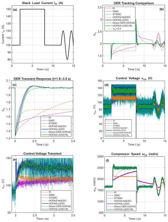
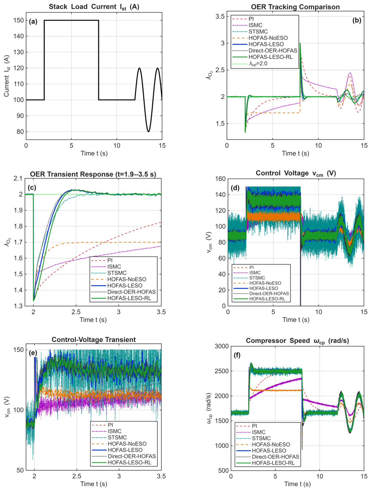
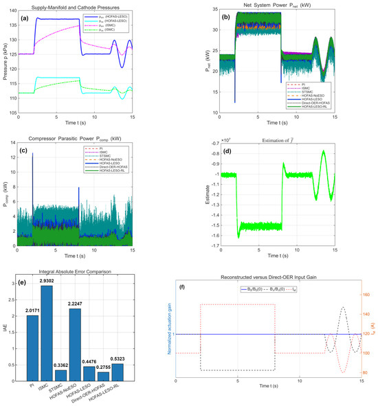
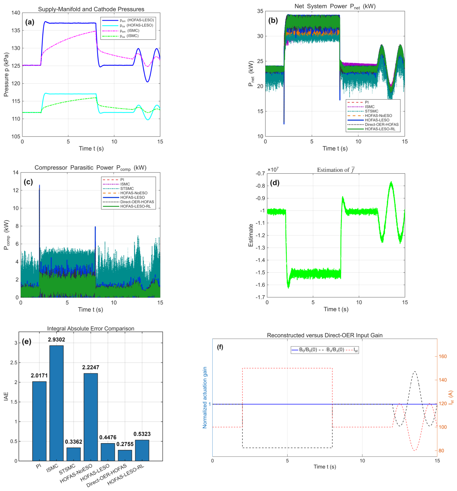
Figure 3 and Figure 4 show the responses. Table 6 reports integral absolute error (IAE), integral time-weighted absolute error (ITAE), settling time, mean net power, the steady-window voltage-rate index $\mathrm{std}(\Delta v_{\mathrm{cm}})/\Delta t$ over 5–7 s, and the full-profile maximum $\max |\Delta v_{\mathrm{cm}}|/\Delta t$. Settling time is the first entry into the $\pm 5\%$ OER band that is maintained for 0.5 s within the first constant-load segment $2\le t<8$ s; a controller that does not satisfy this criterion before the next load change is reported as N/A.

Figure 3. Control responses under 20% parameter perturbation and multiplicative 1% OER/pressure-difference measurement noise: (a) imposed stack-current profile; (b) full-horizon OER tracking for all controllers; (c) enlarged OER transient around the 100–150 A step; (d) full-horizon compressor voltage; (e) enlarged voltage transient; and (f) compressor-shaft speed. The green dotted line in panels (b,c) is the reference ${\lambda }_{\mathrm{ref}}=2$.

Figure 4. Physical and performance diagnostics under the perturbed and noisy condition: (a) supply-manifold and cathode pressures for HOFAS–LESO and ISMC; (b) net system power for all controllers; (c) compressor parasitic power; (d) LESO total-disturbance estimate for $\overline{f}$; (e) IAE comparison; and (f) normalized reconstructed and direct-OER actuation gains together with stack current. Panel (f) shows the constant reconstructed gain versus the $I_{\mathrm{st}}^{-1}$-dependent direct gain.

For readability, Figure 3 uses a conventional two-column, three-row panel grid. The panels are exported independently at 600 dpi with a common footprint, and the shared caption identifies the six panels without repeating text below each image.

In Figure 3, panels (a–c) isolate the imposed load and the resulting OER transients, while panels (d–f) show the voltage effort and the associated compressor-speed response. The paired full-horizon and zoomed panels make the step response and the later sinusoidal-load behavior readable at the final print width.

The multi-controller legends in Figure 3 use one fixed order throughout: PI, ISMC, STSMC, HOFAS-NoESO, HOFAS-LESO, Direct-OER-HOFAS, and HOFAS-LESO-RL; the reference line is listed separately. The primary reconstructed traces use heavier solid lines, while comparison traces use distinct dashed, dash-dotted, or dotted styles. This fixed ordering and the enlarged legend text allow a curve to be identified consistently between the full-horizon panels and their zoomed counterparts.

Figure 4 separates the physical-state response (a), energy consequences (b,c), observer behavior (d), aggregate tracking error (e), and the structural gain comparison (f). This panel-by-panel presentation explains which evidence supports performance claims and which evidence supports the output-reconstruction argument.

For readability, Figure 4 uses the same conventional two-column, three-row panel grid and 600 dpi independent exports. The figure uses the same controller order and color/line-style mapping as Figure 3. The legend is panel-specific: panel (a) lists only the two pressure comparisons, panels (b,c) list all controllers, panel (d) contains the single LESO estimate, panel (e) prints the numerical IAE values directly above the bars, and panel (f) lists only the two normalized gains and stack current.

HOFAS-LESO reduces IAE by 77.8%, 84.7%, and 79.9% relative to PI, ISMC, and the bias-compensated HOFAS-NoESO ablation, respectively.

The fair NoESO result (IAE 2.2247 and mean net power 26.6375 kW) shows a substantial performance penalty when online disturbance estimation is omitted, while the simulated trajectories remain bounded.

The 0.2480 s HOFAS-LESO settling time is 88.6% shorter than that of PI and 13.3% shorter than that of STSMC.

The relative-degree-consistent, grid-tuned STSMC attains an IAE of 0.3362, 24.9% below that of HOFAS-LESO. This tracking advantage requires a steady-window voltage-rate index of 23341.84 V/s, whereas HOFAS-LESO requires 3221.82 V/s, an 86.2% reduction. STSMC also gives a lower mean net power (26.7279 versus 27.3142 kW). Consequently, the numerical comparison supports a tracking–actuation trade-off and does not support universal tracking superiority of the reconstructed controller.

The gain-scheduled Direct-OER-HOFAS benchmark achieves the best unconstrained numerical tracking, with IAE 0.2755 versus 0.4476 for reconstructed HOFAS-LESO.

This comparison clarifies the scope of the proposed method: output reconstruction is not claimed to dominate an ideal gain-scheduled direct controller in sampled-data simulation.

Rather, Figure 4 shows that $B_{\lambda }$ decreases by 33.3% when current rises from 100 to 150 A, while $B_0$ remains constant; at the ideal step, the direct model also contains nonclassical ${\dot{c}}_I$ and ${\ddot{c}}_I$. These facts prevent the direct benchmark from inheriting the proposed constant-gain continuous-time proof.

The lower direct-controller rate index (2569.37 versus 3221.82 V/s) and slightly higher mean net power (27.3336 versus 27.3142 kW) are also acknowledged. They do not establish a practical advantage for reconstruction under ideal instantaneous current scheduling; rather, they quantify the tracking–actuation trade-off at that favorable benchmark condition. The reconstructed formulation is motivated by a less demanding analytical and implementation contract: it avoids differentiating the load-dependent OER gain and does not require the controller to invert an instantaneous current-dependent coefficient at every sample.

The unconstrained HOFAS-LESO has a full-profile maximum voltage rate of 140,649.86 V/s. Equation (70) reduces this value by 99.29% to exactly 1000 V/s. The cost is an 18.9% increase in IAE, from 0.4476 to 0.5323, and a 0.0280 s increase in settling time; mean net power is essentially unchanged. The rate-limited result therefore demonstrates a concrete accuracy–actuator-feasibility trade-off instead of inferring feasibility from the standard-deviation index alone.

5.4. Computational Complexity

Table 7 gives hand-counted primitive arithmetic operations in one discrete controller update. Because comparisons, memory access, and operation-specific latency are excluded, these counts indicate algorithmic order rather than measured execution time.

Table 7. Approximate per-step arithmetic counts.

Controller	Operations/Step	Relative to PI
PI	4	$1.0\times$
ISMC	31	$7.8\times$
STSMC	34	$8.5\times$
HOFAS-NoESO	35	$8.8\times$
HOFAS-LESO	43	$10.8\times$
Direct-OER-HOFAS	25	$6.2\times$
HOFAS-LESO-RL	47	$11.8\times$

At approximately 43 primitive arithmetic operations per step, HOFAS-LESO remains of the same arithmetic order as the sliding-mode baselines. The limiter adds approximately four comparison/update operations, giving 47 operations per step. These hand counts exclude comparison operations, transcendental-operation latency, memory access, and implementation overhead; they indicate arithmetic order only. A hardware timing study is required before making platform-specific real-time claims.

5.5. Bandwidth Sensitivity

Four configurations are evaluated with the tracking-differentiator bandwidth held at $r_{\mathrm{td}}=80$ rad/s: A, $({\omega }_o,{\omega }_c)=(50,30)$; B, $(75,30)$; C, $(100,30)$; and D, $(75,40)$. Table 8 and Figure 5 illustrate the trade-off and provide the reproducible local check used after the initial selection.

Table 8. HOFAS-LESO bandwidth sensitivity.

Case	${\mathit{\omega }}_{\mathit{o}}$	${\mathit{\omega }}_{\mathit{c}}$	Min. OER	IAE	Mean ${\mathit{P}}_{\mathbf{net}}$ (kW)	Chattering (V/s)
A: low observer bandwidth	50	30	1.3337	0.6307	27.3106	1409.63
B: baseline	75	30	1.3339	0.4476	27.3142	3221.82
C: high observer bandwidth	100	30	1.3339	0.3644	27.2343	6114.04
D: high control bandwidth	75	40	1.3340	0.3585	27.2993	4211.02

Note: Bold values indicate the most favorable result in the corresponding metric: the largest minimum OER or mean net power, and the smallest IAE or voltage-rate chattering index.

Figure 5. Bandwidth sensitivity of HOFAS–LESO: (a) OER trajectories for the four observer/controller bandwidth configurations; (b) corresponding compressor-voltage trajectories; and (c) the IAE versus voltage-rate chattering-index trade-off, with labels A–D matching Table 8.

In Figure 5, panel (a) shows tracking changes caused by bandwidth selection, panel (b) shows the voltage activity that produces those changes, and panel (c) summarizes the accuracy–smoothness trade-off as a two-dimensional point set.

Increasing ${\omega }_o$ from 50 to 75 reduces IAE from 0.6307 to 0.4476, whereas increasing it to 100 raises the voltage-rate index by 89.8% relative to the baseline and reduces net power. Increasing ${\omega }_c$ from 30 to 40 improves IAE to 0.3585 but raises the voltage-rate index by 30.7%. Thus, the bandwidths have transparent but non-negligible tracking/noise trade-offs.

5.6. Robustness to Parameter Perturbations

The inertia is increased and the manifold restriction is decreased simultaneously by 0%, 10%, 20%, 30%, and 50%. The same multiplicative 1% noise sequences remain active. Each case is initialized with its own equilibrium pressure difference rather than reusing the 20% case.

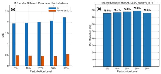
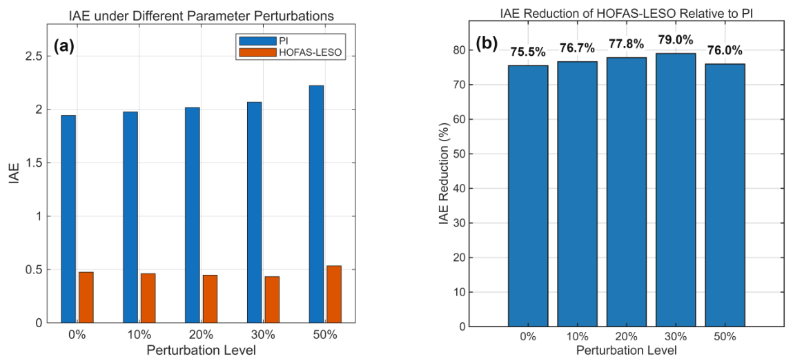
Figure 6 uses panel (a) to report the two controller errors on a common scale and panel (b) to normalize the comparison by the PI baseline. The numerical values are also retained in Table 9 for exact reading.

Figure 6. Robustness to simultaneous compressor-inertia and manifold-restriction perturbations: (a) absolute IAE of PI and HOFAS–LESO at 0%, 10%, 20%, 30%, and 50% perturbation; and (b) the corresponding percentage reduction in IAE achieved by HOFAS–LESO relative to PI.

Table 9. IAE under multiple parameter-perturbation levels.

Perturbation	PI IAE	HOFAS-LESO IAE	Reduction
0%	1.9439	0.4761	75.5%
10%	1.9768	0.4616	76.7%
20%	2.0171	0.4476	77.8%
30%	2.0677	0.4341	79.0%
50%	2.2224	0.5344	76.0%

HOFAS-LESO retains a 75.5–79.0% IAE reduction relative to PI through 30% simultaneous perturbation and a 76.0% reduction at 50%. Its IAE remains within 0.4341–0.5344. Each perturbation case is initialized at its own physical equilibrium, while the controller retains nominal $B_0$ and the same bandwidths.

5.7. Statistical and Time-Step Validation

Table 10 reports the 30-realization Monte Carlo results. The confidence intervals are narrow relative to the separation between controller means, and their ordering agrees with the fixed-seed comparison: Direct-OER-HOFAS gives the lowest IAE, followed by STSMC, HOFAS-LESO, and the rate-limited HOFAS-LESO-RL. Thus, the tracking ranking reported in Table 6 is not attributable to the selected seed 42. The Monte Carlo test addresses measurement-noise repeatability at the fixed 20% plant mismatch; it does not represent a probability distribution over physical parameters.

Table 10. Monte Carlo IAE statistics for 30 independent 1% measurement-noise realizations.

Controller	Mean IAE	Standard Deviation	95% CI for Mean
STSMC	0.3331	0.0040	[0.3317, 0.3346]
HOFAS-LESO	0.4489	0.0014	[0.4484, 0.4494]
Direct-OER-HOFAS	0.2761	0.0013	[0.2756, 0.2766]
HOFAS-LESO-RL	0.5298	0.0052	[0.5279, 0.5316]

Note: Bold values indicate the smallest mean IAE and standard deviation among the compared controllers.

The noise-free convergence results in Table 11 refer to the complete discretized algorithm, including Euler updates of the LESO, adaptive filters, and tracking differentiator, together with RK4 integration of the plant. Relative to the 0.5 ms result, the 1 ms setting changes IAE by 0.3702% and has a maximum pointwise OER difference of $6.06\times {10}^{-3}$. The 2 ms setting gives larger but still bounded differences. This supports the selected 1 ms step as a numerically resolved setting for the reported model; it is not a formal convergence-order estimate because the input contains aligned ideal steps and the controller contains saturation.

Table 11. Noise-free time-step convergence of HOFAS-LESO.

$\mathbf{\Delta }\mathit{t}$ (ms)	IAE	IAE Difference from 0.5 ms	Max. OER Difference
2.0	0.436897	1.2539%	$2.0093\times {10}^{-2}$
1.0	0.433084	0.3702%	$6.0568\times {10}^{-3}$
0.5	0.431487	0	0

5.8. Sensor and Actuator Nonidealities

The validation quantities are reported in Table 10, Table 11 and Table 12. The former compact three-panel validation graphic is replaced by these tables because each protocol contains a small set of aggregate data points; the tabular format gives the exact means, confidence intervals, convergence differences, and nonideality values without duplicating the data.

Table 12. HOFAS-LESO performance under illustrative sensing and actuation nonidealities.

Scenario	IAE	Min. OER	Settling (s)	Mean ${\mathit{P}}_{\mathbf{net}}$ (kW)	Max. Rate (V/s)
Baseline	0.4476	1.3339	0.2480	27.3142	140,649.86
Sensor bias	0.5339	1.3272	0.2540	27.2865	139,895.21
5 ms measurement delay	0.4542	1.3339	0.2470	27.3127	141,475.52
10 ms actuator lag	0.4876	1.3341	0.2630	27.3310	12,910.09
Combined	0.5784	1.3275	0.2690	27.3011	13,173.20

Table 12 summarizes the sensing and actuation stress tests. The 5 ms delay alone increases IAE by only 1.5%, whereas the 10 ms actuator lag increases it by 8.9% and substantially lowers the maximum applied-voltage rate. The adverse sensor-bias combination increases IAE by 19.3%, confirming that the adaptive reference is more sensitive to persistent calibration error than to the tested short delay. Under all three nonidealities simultaneously, IAE is 0.5784, the minimum OER is 1.3275, and settling time increases from 0.2480 to 0.2690 s. The trajectories remain finite and within the 0–150 V and positive-pressure/OER domains, but this test does not establish robustness for arbitrary bias, delay, or unmodeled actuator dynamics.

Because the direct benchmark schedules $B_{\lambda }$ with the measured current, we repeat the same stress cases for Direct-OER-HOFAS. Its IAE is 0.2755 in the ideal case, 0.2755 with a 0.5% current bias, 0.2874 with a 5 ms measurement delay, and 0.4145 under the combined $+0.5\%$ OER bias, $+0.5\%$ current bias, 5 ms delay, and 10 ms actuator lag. Direct-OER-HOFAS therefore remains numerically competitive, and sometimes superior, in these mild sampled-data tests. These results do not imply universal numerical superiority: the practical rationale for reconstruction is the elimination of exact instantaneous gain scheduling and the associated nonsmooth load-derivative terms, while its performance benefit under hardware-calibrated uncertainty remains an empirical question.

5.9. WLTC-like Multisegment Load Profile

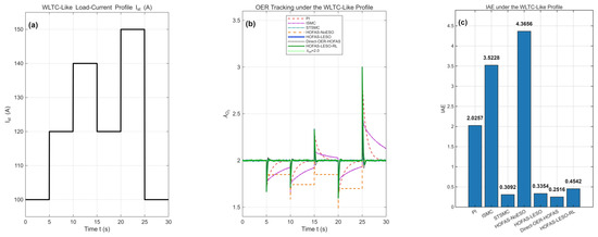
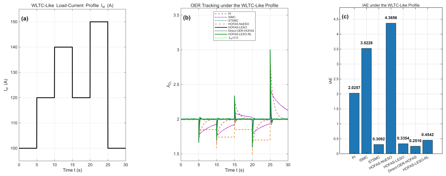
A 30 s profile contains 100 A (0–5 s), 120 A (5–10 s), 140 A (10–15 s), 120 A (15–20 s), 150 A (20–25 s), and 100 A (25–30 s). This is a WLTC-like multisegment stress profile, not a standardized WLTC current trace derived from a vehicle speed-to-power map.

In Figure 7, panel (a) identifies the six load transitions, panel (b) shows the transient and inter-segment OER behavior, and panel (c) reports the aggregate tracking cost that is listed numerically in Table 13.

Figure 7. WLTC-like multisegment validation: (a) imposed stack-current sequence with six constant-load segments; (b) OER trajectories of all controllers and the ${\lambda }_{\mathrm{ref}}=2$ target; and (c) controller-wise IAE over the complete 30 s profile. The profile is deliberately labeled WLTC-like because it is synthetic rather than a standardized vehicle-cycle current trace.

Table 13. Performance under the WLTC-like load profile.

Controller	IAE	Mean ${\mathit{P}}_{\mathbf{net}}$ (kW)	Rate Index (V/s)	Max. Rate (V/s)
PI	2.0257	27.5329	440.60	15,660.96
ISMC	3.5228	27.3965	5794.64	133,024.70
STSMC	0.3092	26.9173	20,853.90	150,000.00
HOFAS-NoESO	4.3656	26.9145	3378.77	110,142.35
HOFAS-LESO	0.3354	27.5762	2895.97	129,756.80
Direct-OER-HOFAS	0.2516	27.5829	2195.03	78,586.45
HOFAS-LESO-RL	0.4542	27.5939	909.05	1000.00

Note: Bold values indicate the most favorable result in the corresponding metric: the smallest IAE, rate index, or maximum rate, and the largest mean net power.

The reconstructed HOFAS-LESO reduces IAE by 83.4%, 90.5%, and 92.3% relative to PI, ISMC, and the bias-compensated HOFAS-NoESO, respectively. Grid-tuned STSMC gives a slightly lower IAE (0.3092 versus 0.3354), but its voltage-rate index is 7.2 times that of HOFAS-LESO and it reaches the full 150,000 V/s sample-to-sample magnitude limit. Direct-OER-HOFAS again gives the smallest unconstrained IAE. HOFAS-LESO-RL retains an IAE of 0.4542 and enforces the 1000 V/s limit at every load transition. The NoESO comparison supports the value of online disturbance estimation without relying on an incorrectly zero-biased ablation.

6. Discussion

The main contribution is the model structure produced by output selection. Direct OER differentiation embeds $I_{\mathrm{st}}^{-1}$ in the actuation gain, whereas pressure-difference reconstruction leaves a constant nominal gain and moves load dependence to reference generation and an additive disturbance channel. This structure better matches HOFAS pole assignment and LESO disturbance estimation.

Relation to the recent nonlinear-observer HOFAS literature. Li et al. [23] provide the most direct recent precedent in this application area by combining a nonlinear observer with an HOFAS air-supply controller for a fuel-cell subsystem. Their work and the present study emphasize different design levers: nonlinear observation addresses how state and uncertainty information is injected into the HOFAS coordinates, whereas the present output reconstruction addresses where the load current appears in the input channel. The latter distinction remains relevant even if a nonlinear observer is adopted, because an OER-output formulation still carries the factor $c_I\propto I_{\mathrm{st}}^{-1}$ and its load derivatives. Accordingly, the present LESO results should be interpreted as a constant-nominal-gain baseline and a structural analysis complementary to, rather than a performance replacement for, nonlinear-observer HOFAS control.

The direct benchmark sharpens the scope of this contribution. With exact current scheduling and discrete-time saturation, it outperforms the reconstructed controller in IAE; therefore, the numerical evidence does not support a blanket performance-superiority claim for output reconstruction. Its advantage comes with a time-varying gain, an instantaneous OER jump under ideal current steps, and disturbance terms containing load-current derivatives. The proposed reconstruction instead offers a constant nominal gain and a continuous pressure state through an ideal current step, which are the ingredients used in the UUB argument. The two formulations consequently trade sampled-data tracking performance against analytical regularity.

Interpretation boundary. The UUB theorem applies only to a forward-complete continuous-time solution with a smooth load, bounded lumped-disturbance derivative, noise-free output, unsaturated input, and operation inside the stated smooth compressor region. Ideal load steps, sensor noise, magnitude or rate saturation, delays, biases, and actuator lag violate one or more of these hypotheses. The corresponding digital simulations are therefore engineering stress tests and implementation checks; they do not prove UUB for the non-ideal loop, nor can they substitute for hardware-in-the-loop or experimental verification based on calibrated sensors, measured compressor maps, and device-specific actuator limits.

The current-sensor delay has a particularly direct effect on the gain-scheduled benchmark. Let $I_m\left(t\right)=I_{\mathrm{st}}(t-{\tau }_I)$ be the current used by Direct-OER-HOFAS and let $\kappa >0$ collect the constant factors in Equation (69). The scheduled and actual OER actuation coefficients are then $B_{\lambda ,\mathrm{used}}=\kappa /I_m$ and $B_{\lambda ,\mathrm{true}}=\kappa /I_{\mathrm{st}}$, respectively.

$${\displaystyle \frac{B_{\lambda ,\mathrm{used}}}{B_{\lambda ,\mathrm{true}}}}-1={\displaystyle \frac{I_{\mathrm{st}}\left(t\right)}{I_{\mathrm{st}}(t-{\tau }_I)}}-1\approx {\tau }_I{\displaystyle \frac{{\dot{I}}_{\mathrm{st}}\left(t\right)}{I_{\mathrm{st}}\left(t\right)}},{\tau }_I\ll {\displaystyle \frac{I_{\mathrm{st}}}{|{\dot{I}}_{\mathrm{st}}|}}.$$

(72)

Thus, during a rising-current transient, the delayed schedule overestimates $B_{\lambda }$ and the applied voltage is insufficient for the actual plant; during a falling transient, the opposite mismatch occurs. In the reconstructed method, $B_0$ remains constant, and a delayed current enters the adaptive-reference path through $y_d={\widehat{k}}_d{I}_m$, producing a reference mismatch and transient lag rather than the instantaneous multiplicative inversion $I_m/I_{\mathrm{st}}$ in Equation (72). Under the common 5 ms delay test used here (which delays all three measured signals), the IAE of Direct-OER-HOFAS increases from 0.2755 to 0.2874 (about 4.3%), whereas that of the reconstructed HOFAS–LESO increases from 0.4476 to 0.4542 (about 1.5%). These values are illustrative combined-delay results, not an isolated identification of the current-sensor delay; a hardware-specific delay tolerance requires a separate sensor and actuator timing model.

Within the reconstructed architecture, the bias-compensated HOFAS-NoESO ablation retains the constant gain but has an IAE nearly five times that of HOFAS-LESO, showing that online disturbance estimation materially improves performance under mismatch. This comparison does not use an artificially zero-biased controller. The rate-limited variant further shows that the observer/controller can be implemented with a hard input-rate bound when the applied voltage is fed back to the LESO.

The modest tracking penalty of this variant supports reporting actuator feasibility explicitly rather than inferring it from an average activity metric.

Several limitations should qualify the results.

First, Theorem 1 is conditional: it assumes a bounded lumped-disturbance derivative under smooth loads and does not establish UUB of the noisy, saturated, ideal-step OER loop or global boundedness of the implemented input. Lemma 1 establishes internal-state boundedness only along a forward-complete solution that remains in the smooth compressor region; it does not prove positive invariance of the physical pressure and speed constraints. Corollary 2 additionally requires the stack current to remain uniformly positive and preserves, rather than suppresses, the ultimate reference-generation mismatch.

Second, the thermodynamic model is control-oriented and omits humidity, temperature transients, gas composition dynamics, measured compressor maps, and coupled thermal and water-management states.

Third, the 0.5% biases, 5 ms delay, and 10 ms first-order actuator lag are illustrative stress-test values rather than hardware-identified uncertainty bounds; the observed bias sensitivity requires calibration and drift evaluation with real sensors.

Fourth, 1000 V/s is an illustrative rate limit because no specific compressor-drive datasheet is assumed; hardware-specific magnitude, current, thermal, and slew constraints must replace this illustrative value in deployment.

Fifth, the direct benchmark assumes instantaneous current scheduling; the added bias/delay/lag sensitivity test is informative but remains an illustrative finite-case study, not a hardware uncertainty envelope.

Sixth, the 30-trial Monte Carlo study varies only the Gaussian measurement noise while holding the plant mismatch fixed and therefore does not quantify joint uncertainty in physical parameters, operating temperature, or model form.

Finally, the WLTC-like profile is not a standardized drive-cycle current trace.

Future work should include hardware-in-the-loop validation, measured compressor maps, hardware-calibrated sensor drift and latency tests, and multivariable regulation using compressor voltage and back-pressure-valve opening. A two-input fully actuated formulation could jointly regulate OER and membrane differential pressure while enforcing actuator constraints.

7. Conclusions

This study develops a state-space-reconstructed HOFAS-LESO controller for PEMFC OER regulation. Selecting $p_{\mathrm{sm}}-p_{\mathrm{ca}}$ as the controlled output removes load current from the nominal actuation coefficient. The actual gain mismatch is absorbed into the total disturbance and estimated by a third-order LESO. Under explicitly stated smooth-load, bounded-disturbance-derivative, and unsaturated-input assumptions, a composite Lyapunov proof establishes UUB of the pressure-difference tracking and observer errors. A conditional internal-dynamics lemma then establishes bounded pressure and compressor-speed states within the smooth operating region, and an OER-error corollary quantifies how the pressure-difference bound and reference-generation mismatch propagate to the regulated output when stack current is bounded away from zero. These results establish neither unconditional global stability nor positive invariance in the physical operating region.

The conclusions must therefore be interpreted conditionally. The proof does not cover ideal step loads, noisy measurements, voltage magnitude or slew saturation, delays, biases, actuator lag, or arbitrary excursions outside the smooth operating region. The noisy, saturated, stepped, and rate-limited digital cases reported in this manuscript demonstrate finite-case implementation behavior and performance trade-offs only; they are not substitutes for hardware-in-the-loop or experimental verification. Hardware-specific sensor latency and calibration, measured compressor characteristics, and device-specific voltage, current, thermal, and slew constraints remain necessary before claiming deployment-level robustness.

A separate smooth-load, noise-free, and unconstrained check keeps the commanded voltage within $[68.8947,108.0243]$ V and yields an IAE of 1.112215. This case is the numerical consistency check associated with the theorem hypotheses; the remaining noisy, saturated, stepped, rate-limited, delayed, biased, and lagged cases are engineering stress tests outside those hypotheses.

The matched current-scheduling sensitivity test gives Direct-OER-HOFAS an IAE of 0.4145 under the combined sensor bias, 5 ms delay, and 10 ms actuator lag, compared with 0.5784 for HOFAS-LESO. In the common 5 ms measurement-delay case, the IAE of the direct benchmark increases by about 4.3% relative to its ideal value, compared with a 1.5% increase in the IAE of the reconstructed HOFAS–LESO controller; this difference is consistent with the delayed-current gain mismatch in Equation (72), although the test is not an isolated current-delay experiment. Thus, even after adding these nonidealities, the simulations do not establish numerical dominance of reconstruction; the claimed contribution is structural regularity and reduced dependence on exact current scheduling.

Under 20% parameter perturbation and multiplicative 1% measurement noise, reconstructed HOFAS-LESO achieves an IAE of 0.4476, a 0.2480 s settling time, and a mean net power of 27.3142 kW. It improves substantially over PI, ISMC, and the bias-compensated NoESO ablation. A relative-degree-consistent, grid-tuned STSMC achieves a lower IAE of 0.3362, but HOFAS-LESO reduces its steady-window voltage-rate index by 86.2%. The gain-scheduled direct-OER benchmark gives the lowest unconstrained IAE of 0.2755, but its nominal gain changes by 33.3% across the 100–150 A step, and its continuous-time step-load derivatives are not classically bounded. These comparisons identify analytical regularity and a tracking–actuation trade-off, rather than universal numerical dominance, as the benefit of reconstruction. The rate-limited implementation enforces a 1000 V/s maximum with an IAE of 0.5323 and a settling time of 0.2760 s. Thirty independent noise realizations give HOFAS-LESO an IAE of $0.4489\pm 0.0014$; the selected 1 ms step differs by 0.3702% in noise-free IAE from the 0.5 ms result; and the combined illustrative sensing/actuation nonidealities give an IAE of 0.5784. These additions improve numerical reproducibility but do not replace hardware validation with measured compressor maps, calibrated sensors, and device-specific limits.

References

- Pukrushpan, J.T.; Stefanopoulou, A.G.; Peng, H. Control of fuel cell breathing. IEEE Control Syst. Mag. 2004, 24, 30–46. [Google Scholar] [CrossRef] [Scilit]
- Pukrushpan, J.T.; Peng, H.; Stefanopoulou, A.G. Control of Fuel Cell Power Systems: Principles and Applications with MATLAB/Simulink; Springer: London, UK, 2004. [Google Scholar]
- Han, J. Auto-disturbance-rejection controller and its applications. Control Decis. 1998, 13, 19–23. (In Chinese) [Google Scholar]
- Pilloni, A.; Pisano, A.; Usai, E. Observer-based air excess ratio control of a PEM fuel cell system via high order sliding mode. IEEE Trans. Ind. Electron. 2015, 62, 5236–5246. [Google Scholar] [CrossRef] [Scilit]
- Wang, Y.; Li, H.; Feng, H.; Han, K.; He, S.; Gao, M. Simulation study on PEMFC oxygen starvation based on the coupling algorithm of model predictive control and PID. Energy Convers. Manag. 2021, 249, 114851. [Google Scholar] [CrossRef] [Scilit]
- Chen, J.; Liu, Z.; Wang, F.; Ouyang, Q.; Su, H. Optimal oxygen excess ratio control for PEM fuel cells. IEEE Trans. Control Syst. Technol. 2018, 26, 1711–1721. [Google Scholar] [CrossRef] [Scilit]
- Deng, H.; Li, Q.; Cui, Y.; Zhu, Y.; Chen, W. Nonlinear controller design based on cascade adaptive sliding mode control for PEM fuel cell air supply systems. Int. J. Hydrogen Energy 2019, 44, 19357–19369. [Google Scholar] [CrossRef] [Scilit]
- Guo, X.; Fan, N.; Dong, Z.; Wang, C. Adaptive prescribed performance control for PEM fuel cell air supply systems with unknown air compressor faults. IEEE Trans. Ind. Electron. 2024, 71, 7664–7672. [Google Scholar] [CrossRef] [Scilit]
- Wang, Y.; Wang, Y. Pressure and oxygen excess ratio control of PEMFC air management system based on neural network and prescribed performance. Eng. Appl. Artif. Intell. 2023, 121, 105850. [Google Scholar] [CrossRef] [Scilit]
- Duan, F.; Kang, Z. Oxygen excess ratio feedforward control based on ESO for PEMFC in DC off-grid hydrogen production systems. Int. J. Hydrogen Energy 2024, 77, 347–358. [Google Scholar] [CrossRef] [Scilit]
- Liu, J.; Gao, Y.; Su, X.; Wack, M.; Wu, L. Disturbance-observer-based control for air management of PEM fuel cell systems via sliding mode technique. IEEE Trans. Control Syst. Technol. 2019, 27, 1129–1138. [Google Scholar] [CrossRef] [Scilit]
- Kim, B.M.; Choi, Y.H.; Yoo, S.J. Adaptive control of proton exchange membrane fuel cell air supply systems with asymmetric oxygen excess ratio constraints. IEEE Access 2020, 8, 5537–5549. [Google Scholar] [CrossRef] [Scilit]
- Yuan, H.; Dai, H.; Ming, P.; Zhan, J.; Wang, X.; Wei, X. A fuzzy extended state observer-based cascade decoupling controller of air supply for vehicular fuel cell system. Energy Convers. Manag. 2021, 236, 114080. [Google Scholar] [CrossRef] [Scilit]
- Duan, G. High-order system approaches I: Fully actuated systems and parametric designs. Acta Autom. Sin. 2020, 46, 1333–1345. (In Chinese) [Google Scholar]
- Duan, G. High-order fully actuated system approaches: Part I. Models and basic procedure. Int. J. Syst. Sci. 2021, 52, 422–435. [Google Scholar] [CrossRef] [Scilit]
- Duan, G. High-order system approaches II: Controllability and full-actuation. Acta Autom. Sin. 2020, 46, 1571–1581. (In Chinese) [Google Scholar]
- Duan, G. High-order system approaches III: Observability and observer design. Acta Autom. Sin. 2020, 46, 1885–1895. (In Chinese) [Google Scholar]
- Wang, X.; Duan, G. High-order fully actuated system approaches: Model predictive control with applications to under-actuated systems. J. Frankl. Inst. 2023, 360, 6953–6975. [Google Scholar] [CrossRef] [Scilit]
- Lu, S.; Tsakalis, K.; Chen, Y. High-order fully actuated system approach for quadrotor control based on extended state observers. Int. J. Syst. Sci. 2025, 56, 3194–3215. [Google Scholar] [CrossRef] [Scilit]
- Yu, Y.; Liu, G.P.; Huang, Y.; Guerrero, J.M. Distributed learning-based secondary control for islanded DC microgrids: A high-order fully actuated system approach. IEEE Trans. Ind. Electron. 2024, 71, 2990–3000. [Google Scholar] [CrossRef] [Scilit]
- Liu, W.; Duan, G.; Hou, M.; Golestani, M.; Kong, H. Control of uncertain high-order fully actuated strict-feedback systems: A backstepping approach with high-gain observer-based derivative approximation. IEEE Trans. Cybern. 2024, 54, 7456–7468. [Google Scholar] [CrossRef] [Scilit] [PubMed]
- Li, P.; Duan, G.; Zhang, B.; Wang, P.; Wang, Y. High-order fully actuated approach for output tracking control of flexible servo systems subject to uncertainties and disturbances. IEEE Trans. Ind. Electron. 2025, 72, 9433–9443. [Google Scholar] [CrossRef] [Scilit]
- Li, G.; Yao, F.; Zhang, Y.; Gao, J.; Hu, Y. Nonlinear observer-based air supply subsystem control via a high-order fully actuated approach for fuel cell. IEEE Trans. Veh. Technol. 2025, 74, 17136–17148. [Google Scholar] [CrossRef] [Scilit]
- Amphlett, J.C.; Baumert, R.M.; Mann, R.F.; Peppley, B.A.; Roberge, P.R. Performance modeling of the Ballard Mark IV solid polymer electrolyte membrane fuel cell. J. Electrochem. Soc. 1995, 142, 1. [Google Scholar] [CrossRef] [Scilit]
- Wang, C.; Nehrir, M.H.; Shaw, R.R. Dynamic models and model validation for PEM fuel cells using electrical circuits. IEEE Trans. Energy Convers. 2005, 20, 442–451. [Google Scholar] [CrossRef] [Scilit]
- Han, J. From PID to active disturbance rejection control. IEEE Trans. Ind. Electron. 2009, 56, 900–906. [Google Scholar] [CrossRef] [Scilit]
- Gao, Z. Scaling and bandwidth-parameterization based controller tuning. In Proceedings of the 2003 American Control Conference, Denver, CO, USA, 4–6 June 2003; pp. 4989–4996. [Google Scholar]
- Chen, W.H.; Yang, J.; Guo, L.; Li, S. Disturbance-observer-based control and related methods: An overview. IEEE Trans. Ind. Electron. 2016, 63, 1083–1095. [Google Scholar] [CrossRef] [Scilit]
- Guo, B.Z.; Zhao, Z.L. On the convergence of an extended state observer for nonlinear systems with uncertainty. Syst. Control Lett. 2011, 60, 420–430. [Google Scholar] [CrossRef] [Scilit]
- Huang, Y.; Xue, W. Active disturbance rejection control: Methodology and theoretical analysis. ISA Trans. 2014, 53, 963–976. [Google Scholar] [CrossRef] [Scilit] [PubMed]
- Shtessel, Y.; Taleb, M.; Plestan, F. A novel adaptive-gain supertwisting sliding mode controller: Methodology and application. Automatica 2012, 48, 759–769. [Google Scholar] [CrossRef] [Scilit]
Disclaimer/Publisher’s Note: The statements, opinions and data contained in all publications are solely those of the individual author(s) and contributor(s) and not of MDPI and/or the editor(s). MDPI and/or the editor(s) disclaim responsibility for any injury to people or property resulting from any ideas, methods, instructions or products referred to in the content. |
© 2026 by the authors. Licensee MDPI, Basel, Switzerland. This article is an open access article distributed under the terms and conditions of the Creative Commons Attribution (CC BY) license.