


Abstract
This paper investigates the valuation of fixed-income securities under short-rate dynamics characterised by bimodal probability distributions. In particular, the valuation of zero-coupon bonds under short-rate dynamics provides one of the fundamental links between a model of interest rates and observable prices of fixed-income securities. Traditional term structure models, such as affine diffusion and single-regime stochastic processes, typically assume unimodal distributions for interest rates, limiting their ability to capture environments with persistent clustering around distinct rate levels. Motivated by empirical observations of policy-driven regimes and liquidity segmentation in modern money markets, we introduce a framework in which the short rate exhibits bimodal density that does not rely explicitly on a regime-switching mechanism. We develop a tractable pricing methodology for zero-coupon bonds under this setting, calibrate the solution to real data and numerically validate the solution. We also examine how bimodality influences yield curves. The analysis highlights that bimodal distributions can generate non-standard term-structure shapes that differ from classical models.
MSC:
35R35; 91G50; 91-10
1. Introduction
The valuation of bonds depends critically on how interest rates are modelled over time. Classical short-rate frameworks—beginning with the influential work of Vasicek [1] and the Cox–Ingersoll–Ross, CIR, model [2]—assume that the short rate follows a single regime stochastic process with a unimodal distribution. These models underpin much of modern term structure theory and were later generalised in affine frameworks by researchers such as Duffie and Kan [3] and Goard [4].
These classical models allow analytical tractability for bond and interest rate derivatives and serve as important benchmarks in fixed-income pricing and risk management. A more recent direction in the literature concerns enhancing the dynamics of mean reversion and volatility. Jha [5] proposes a sinusoidal extension of the Hull–White model to capture long-term cyclical behaviour in Treasury yields. Samimi and Najafi [6] assumed that interest-rate dynamics are modelled by a skew Vasicek model and derived analytical pricing formulas for both zero-coupon bonds and European options. Higher-factor models that include stochastic volatility are another active area of research. Recently, Banos et al. [7] have analysed change-of-measure techniques for Heston–Hawkes stochastic volatility systems, which can be important to bond-related pricing. Contemporary research also continues to evaluate the numerical implementation of one-factor models for derivative and bond pricing especially under finite-difference and Monte Carlo methods. See, for example, Lee and Yang [8], who review finite-difference implementations for the one factor Hull–White model; Falco et al. [9], who develop Crank–Nicolson finite-difference schemes for one-factor Hull–White partial differential equations (PDEs) with dynamically consistent forward curves, and Ullah [10], who employs stochastic volatility and advanced finite-difference techniques relevant to the Hull–White implementation. For Monte-Carlo methods, see, for example, Fries [11] and Treepongkaruna and Gray [12].
Empirically however, recent interest rate data suggest that the unimodal assumption may be too restrictive. This is particularly evident when examining post-crisis and post-pandemic rate environments. For example, the US secured overnight funding rate, SOFR, moved from levels of nearly zero (below 0.1%) for extended periods between 2020 and 2021 to above 5% by 2023 following rapid monetary tightening. Similarly, the Euro short-term rate, €STR, has exhibited prolonged clustering near the deposit facility rate before sharply shifting upward during the ECB tightening cycle. In the UK, the Sterling Overnight Index Average (SONIA) has displayed a comparable pattern with extended low-rate regimes followed by abrupt transitions. Even the Islamic Interbank Benchmark Rate (IIBR) (see [13]), designed to calculate the expected return on Sharia-compliant, short-term interbank funding, exhibits bimodal behaviour.
When these series are viewed over a sufficiently long horizon, the empirical distribution of short rates does not appear smoothly unimodal. Instead, rates often cluster around distinct levels corresponding to different monetary policy regimes—such as the post-2008 near-zero rate environment and the post-2022 tightening cycles. This creates a distribution that can plausibly be interpreted as bimodal or at least strongly multi-peaked rather than centred around a single long-run mean.
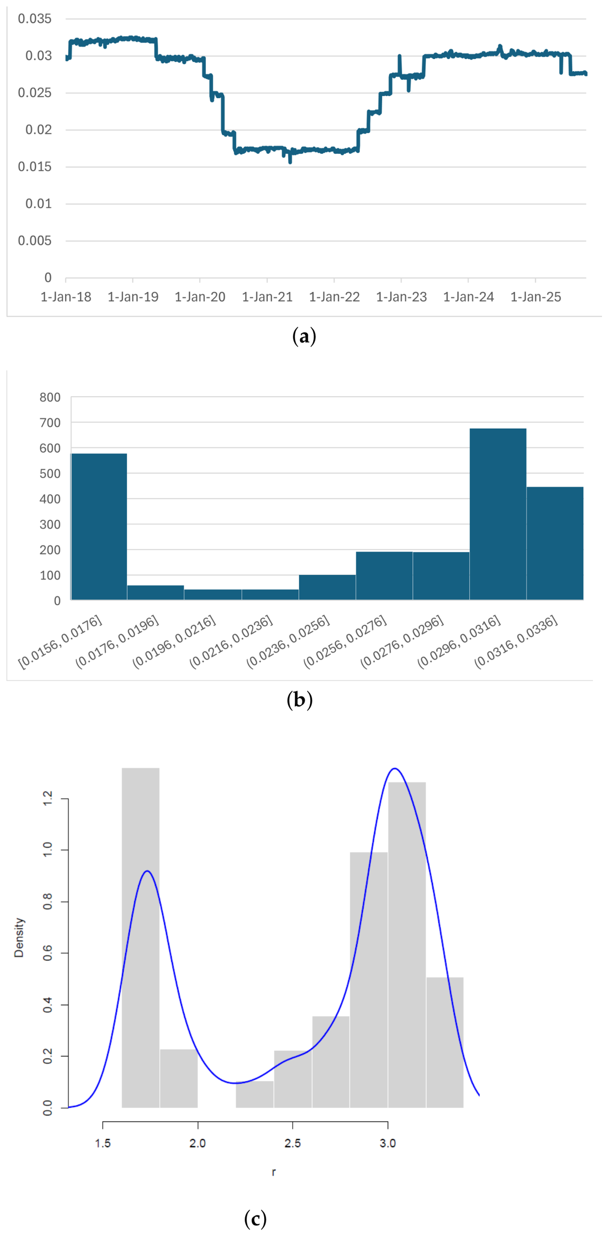
Furthermore, repurchase rates (or repo rates) frequently flip between two distinct levels within the same period. In Appendix A, we plot daily historical data and histograms of a number of short rates. Visual inspections of the histograms with kernel density overlays point to bimodal densities. This is supported by the results of Hartigan’s Dip Test, which measures the departure of the distribution from unimodality. For the datasets tested, though, Silverman’s test suggests that there are more than two modes but is consistent with a situation in which two dominant modes are separated, and any additional modes are relatively minor fluctuations or local bumps. A bimodal model should then capture the primary structure of the data well.
Standard attempts to capture this behaviour typically rely on regime-switching models, as introduced by Hamilton [14]. These frameworks allow the short rate to transition between discrete states, such as low and high regimes, with probabilities governed by a Markov process. Subsequent applications to term structures (e.g., Ang and Bekaert [15] and Siu and Elliott [16]) demonstrate that regime switching can capture shifts between high and low rate environments. However, while successful in capturing structural breaks, these models do not capture all types of bimodal behaviour, and further, they introduce estimation challenges and require explicit assumptions about transition dynamics and state persistence.
An alternative approach is to model the short rate in a way that directly incorporates bimodality in its distribution without explicitly specifying regime transitions. Instead of treating regimes as latent states, the distribution itself reflects two dominant regions of probability mass. This observation is consistent with the observed clustering in many short-rate data, where the rates spend periods are near distinct policy-driven levels rather than varying smoothly around a single mean.
From a bond-pricing perspective, this raises a natural question: how does the presence of a bimodal short-rate distribution affect the valuation of fixed-income securities? In particular, it is unclear whether standard quantities such as yields behave in a predictable way when probability mass is split across two separated rate regions.
This paper investigates bond pricing under a bimodal short-rate specification motivated by these empirical features. We consider a class of models in which the marginal distribution of the short rate has two distinct modes and examine the impact of bimodality itself rather than attributing dynamics to explicit regime switches. We derive an analytic approximation for bond prices even in the presence of a nonlinear drift that generates the bimodal behaviour. We also examine how their structure reshapes the resulting yield curve.
In Section 2, we revisit the regime-switching Hull–White model as investigated by Shen and Siu [17]. Hence, we assume that the mean value of the short rate is subject to random shifts between two states, . represents a stronger economy when interest rates are higher, and represents the state when interest rates are lower. A different mean value to which the rates revert, p, is assumed in each state. Hence, when , then , (with ), and the dynamics of the rate are assumed to follow a stochastic process
where here and in the remainder of this paper, is an increment in a Wiener process Z. We assume that the transition between states occurs as a Poisson process with rate being the transition rate from state 1 to state 2 and being the transition rate from state 2 to state 1.
While the bond price solution under this model is derived by Shen and Siu [17], we provide a solution in a simple, algebraic form using matrix algebra.
In Section 3, we model the short rate by using a single bimodal model—a nonlinear equation but with two stable fixed points, at high and low values of the rate, respectively. One such single-factor model that we consider is
with and constant, the stable low fixed point, the stable high fixed point and an unstable intermediate fixed point. In the neighbourhood of , the rate reverts to as
with time scale . Similarly, in the neighbourhood of , short rates revert to exponentially with a time scale .
For an initial value strictly between and , the full solution to the nonlinear deterministic model is
where
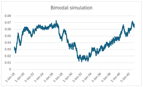
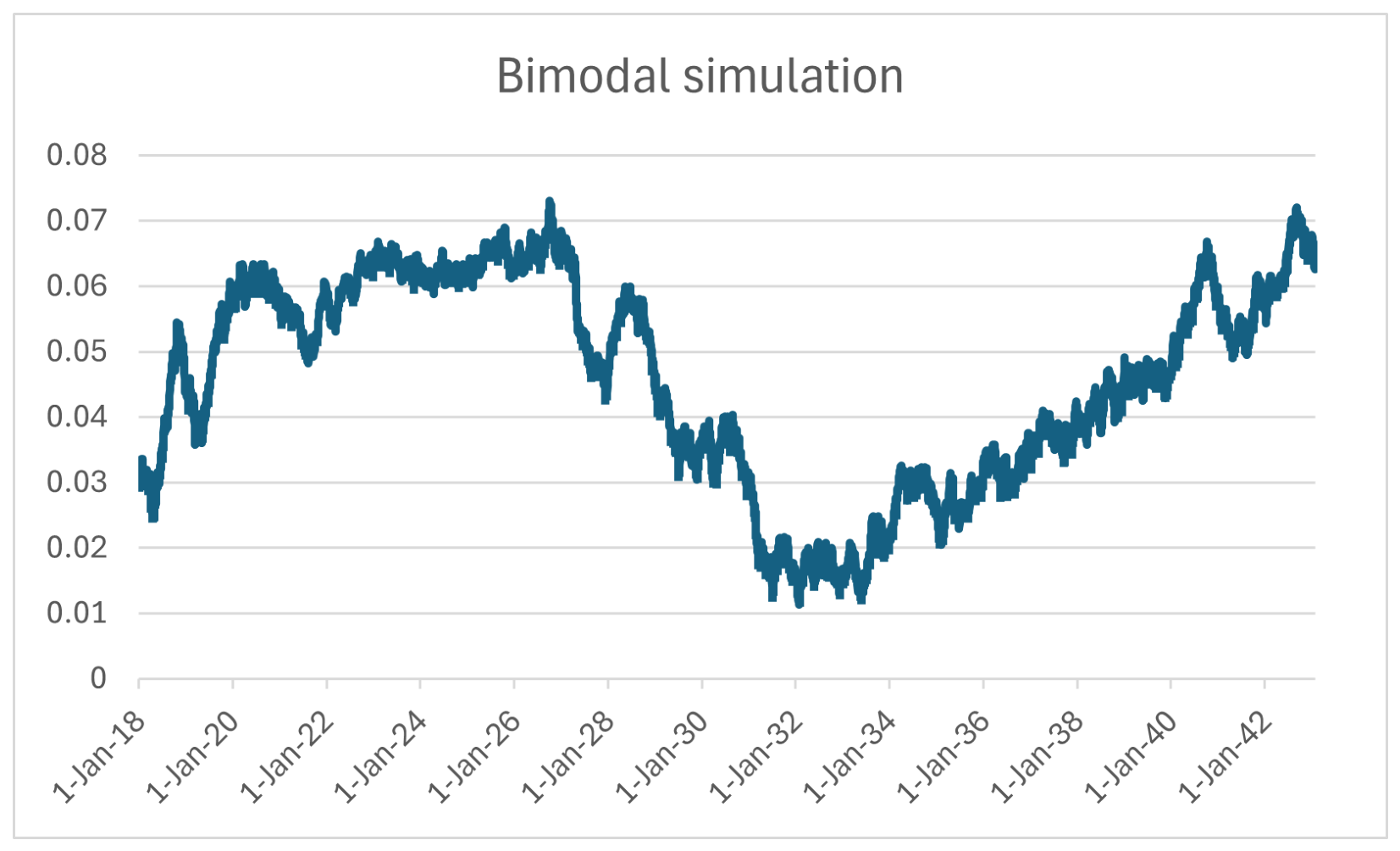
The occasional switching between the low short-rate zone, with interval of attraction , and the high short-rate zone, with interval of attraction , occurs because of the random excursion . Since trajectories spend a large proportion of time near the two stable fixed points, mean residence times for the two zones may be regarded as increasing functions of the step lengths and required to jump from one stable fixed point to the basin of attraction for another. However, this behaviour may be modified by choice of the volatility function. Figure 1 shows a sample simulation of the rates under (2).
Figure 1.
Simulation of model (2) with , , , , and .
Importantly, in Section 3, we find analytic approximations to bonds when the corresponding risk-neutral process for r has a similar form to (2) and with the fixed points equally spaced. This demonstrates how an intrinsic bimodal structure can enhance flexibility in modelling interest rate behaviour. We also validate our solution against a numerical solution and calibrate our model to real data.
2. The Pricing of Bonds Under a Regime-Switching Model
While the valuation of bonds under a regime-switching Hull–White model was considered by Shen and Siu [17], for completeness of valuations under bimodal densities, we revisit the problem and provide a simple and intuitive solution using the partial differential equation (PDE) framework and matrix algebra.
We assume that the mean value of the short rate is subject to random shifts between two states (see Appendix B). Under the assumption of movement of the risk-neutral short rate being described by the process
where, here and in the rest of this paper, is a Wiener process under which the discounted traded asset prices are martingales, then a system of coupled equations for the value of a zero-coupon bond , with expiry T and principal one, can be derived (see Appendix B). This is given by
where , which we solve subject to and as , . We also require to be finite as .
The solution to this system of equations is given in the following Result 1.
Result 1: The fair price of a zero-coupon bond with expiry T and principal 1 under the regime switching model (7) is given by
where
and where
where and are the Kummer-M and Kummer-U functions, respectively.
Proof.
The forms of the initial and boundary conditions suggest solutions of the form
where .
Substituting these forms into (8a) and (8b) and collecting coefficients of powers of r (namely and ), we obtain the following four equations for :
From (13) and (15), we obtain
So that with ,
From (12) and (14), we have
or in matrix form
subject to and where
In the above system, we can eliminate to obtain a single second-order equation for , namely
Then, the solution of can be obtained from (17), i.e.,
Equation (24) is a Confluent Hypergeometric Differential Equation (see e.g., [18]), and its solution is given by
where
Now, we can use (25) to find
Finally, we substitute (26) and (27) into (10) and (11) to obtain (9a) and (9b). □
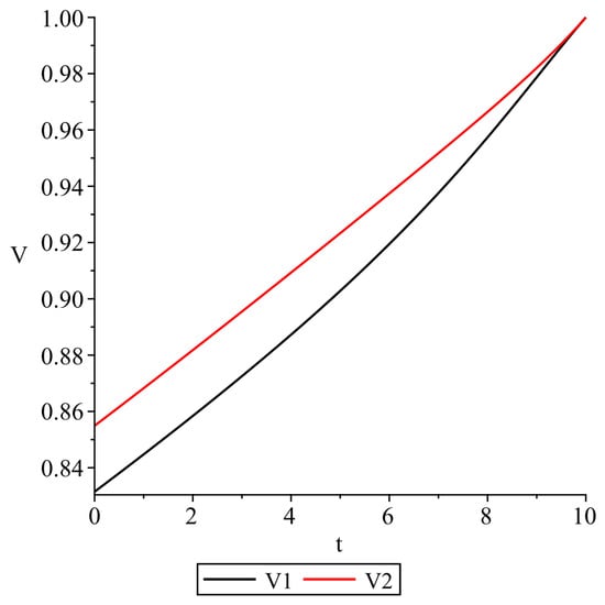
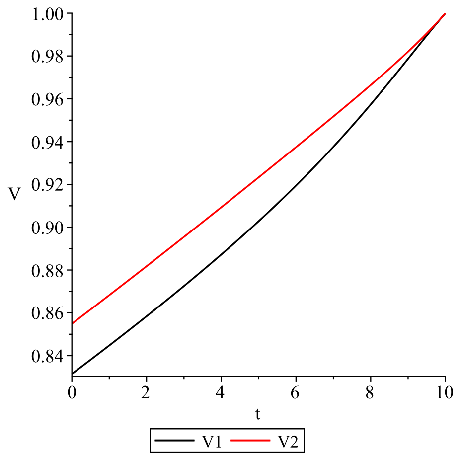
Solutions and are plotted in Figure 2 with the parameters . The solution , which is based on a higher mean-value reversion , is naturally lower than , as higher rates make the bond less attractive and thus lead to lower prices.
Figure 2.
Plots of and as given in Result 1 with , , , , and , , , .
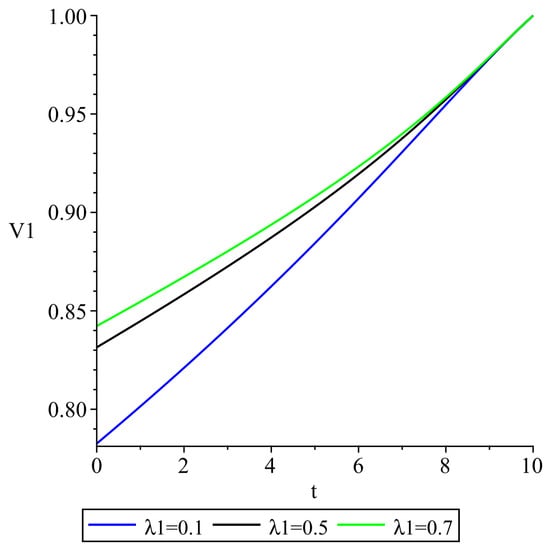
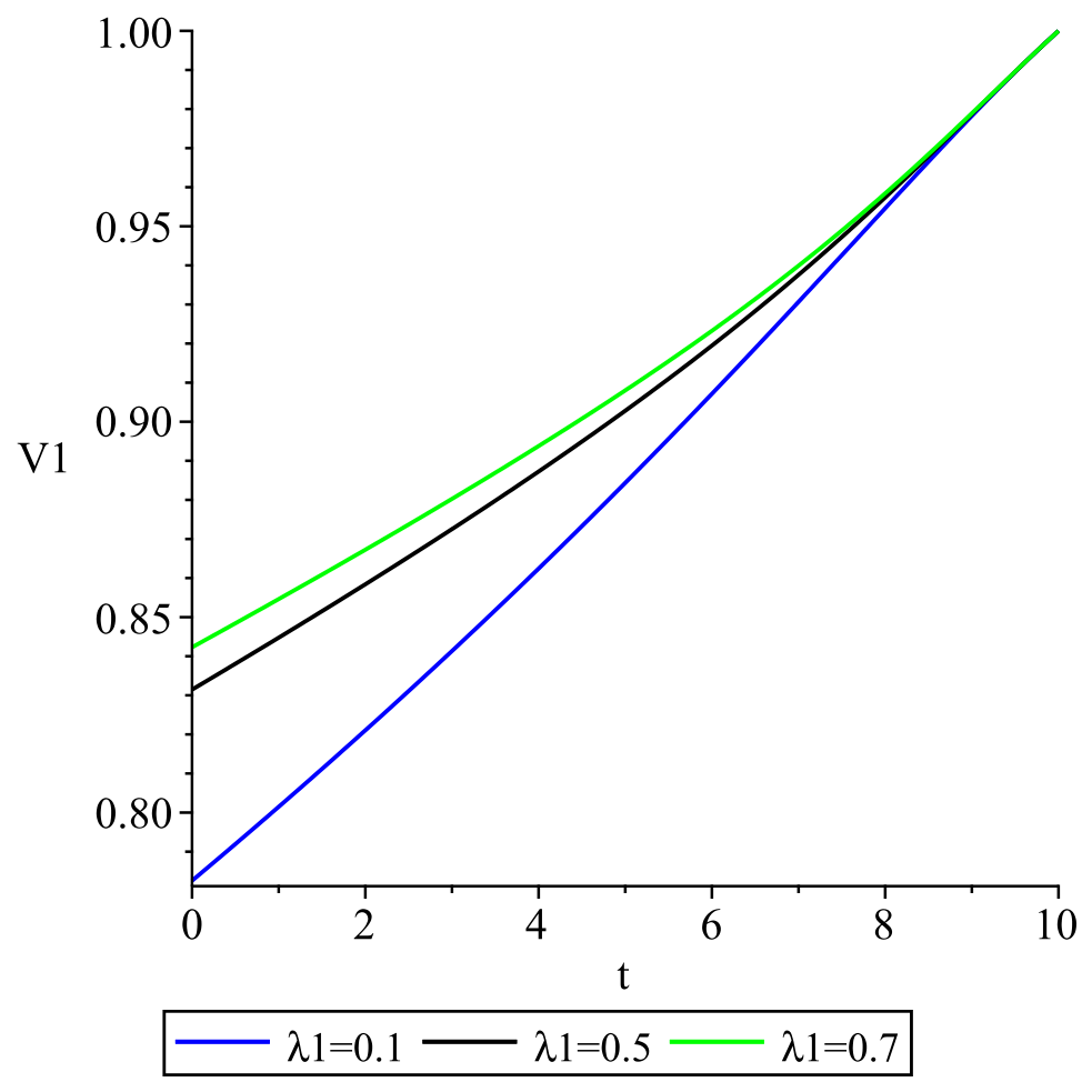
In Figure 3, we plot the solution with held constant and taking on 3 values and . As represents the transition rate from state 1 to state 2, a higher value means more time in state 2 where the mean-value reversion is lower. Hence, a higher value of produces a higher value of .
Figure 3.
Plots of with varying values of and , , , , , , and .
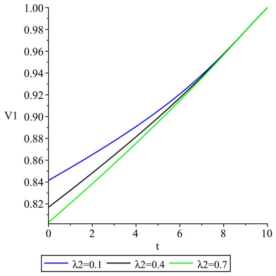
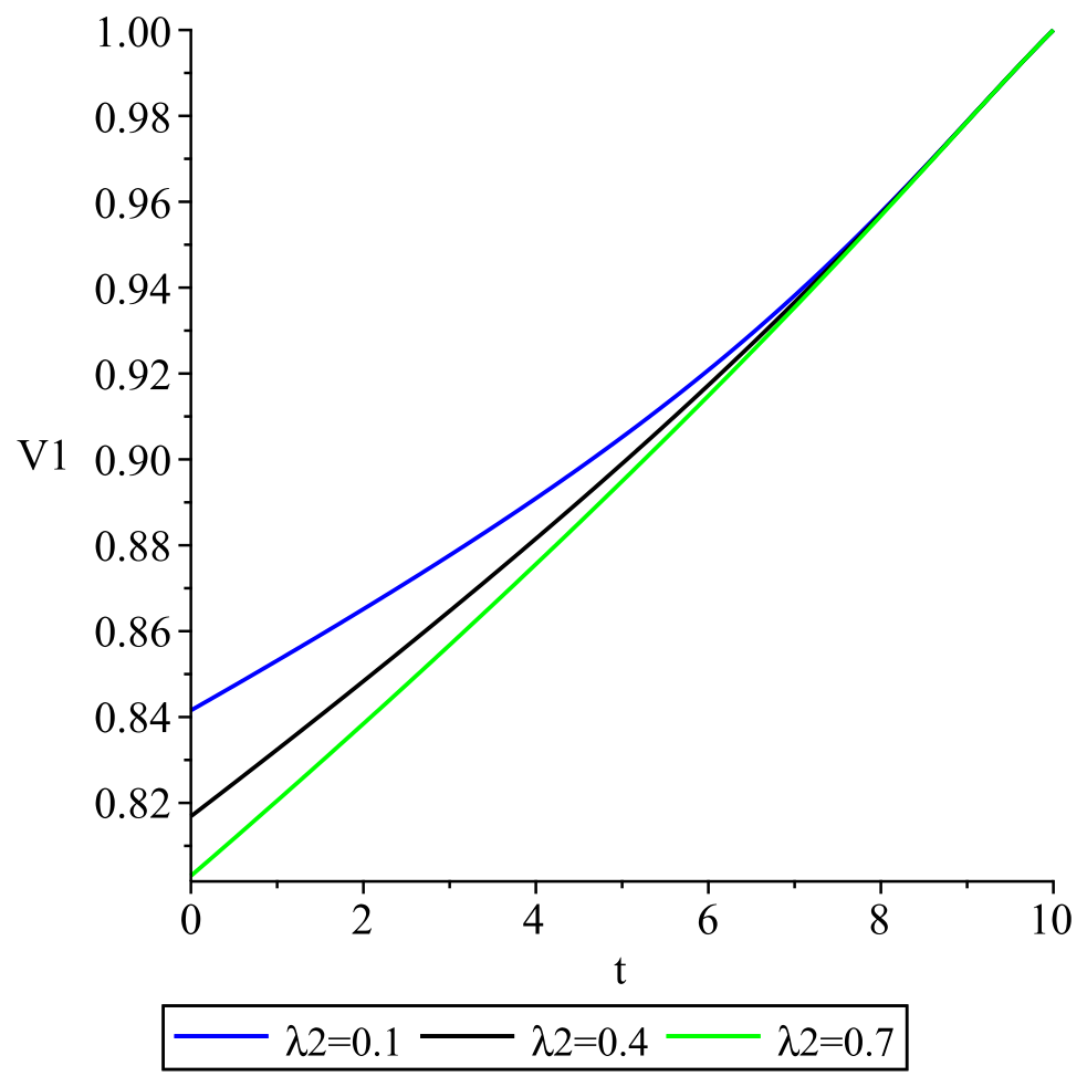
In Figure 4, we plot the solution with held constant and taking on 3 values: , and . The parameter represents the transition rate from state 2 to state 1 so that a higher value means more time in state 1 where the mean-value reversion is higher. Hence, a higher value of produces a lower value .
Figure 4.
Plots of with varying values of and , , , , , , and .
3. Pricing of Bonds Under the Bimodal Model
We now arrive at the main objective of this paper, i.e., to price bonds under a single, nonlinear model.
The partial differential equation (PDE) that governs bond prices with principal and expiry , under the risk-neutral model
is given by (see Appendix C and [19])
where and . We start by non-dimensionalising the problem. This ensures that the relative sizes of different variables is obvious and signifies the important variables and constants in the equation. Hence, we let and . This reduces the problem to
where , and . (Changes of variables include ).
Given that and a are small, then is assumed small (1). Hence, we seek a perturbation solution of the form
where for .
3.1. The O(1) Term
Substituting (31) into (30) and collecting the coefficients of , we find that needs to satisfy
subject to .
In the case or or , from (32), we obtain that
In the following, we assume .
- Solving (32) by the method of characteristics gives
With , we may write
for some function so that . From the initial condition, we require
We now write the LHS of (37) in terms of using (38). After some simplification, we arrive at
and hence
We can simplify this to
for all y.
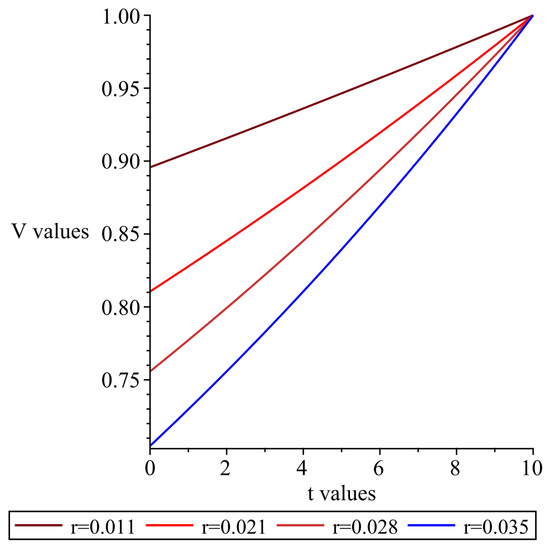
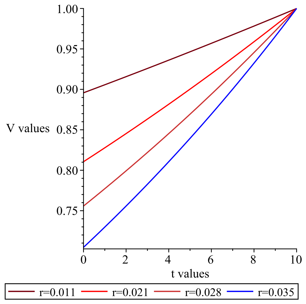
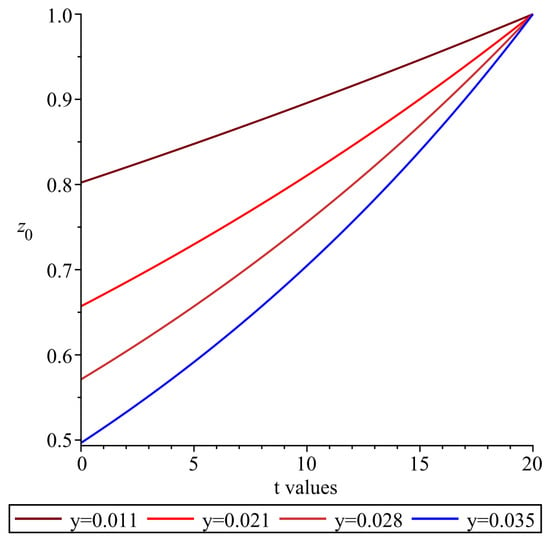
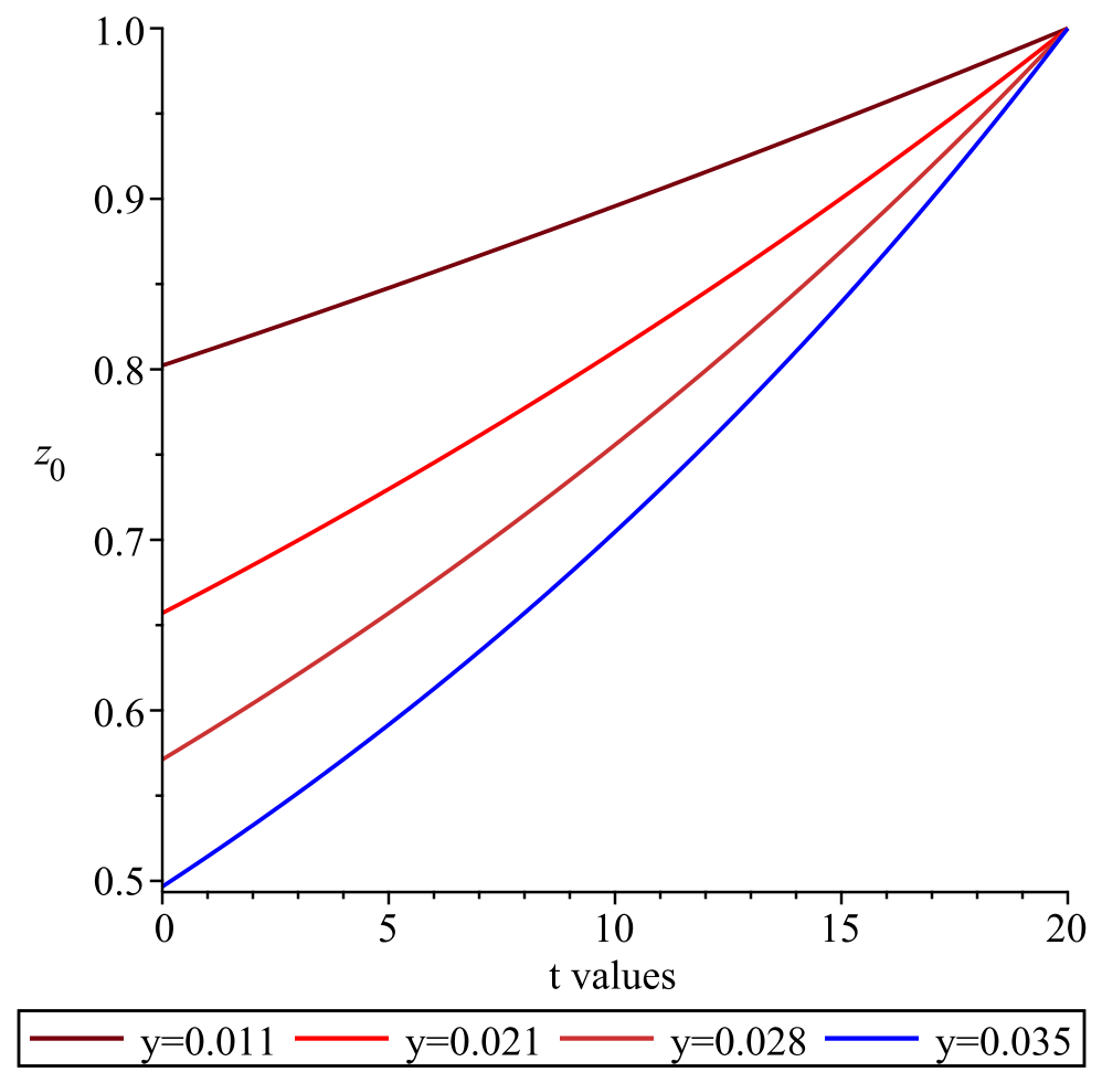
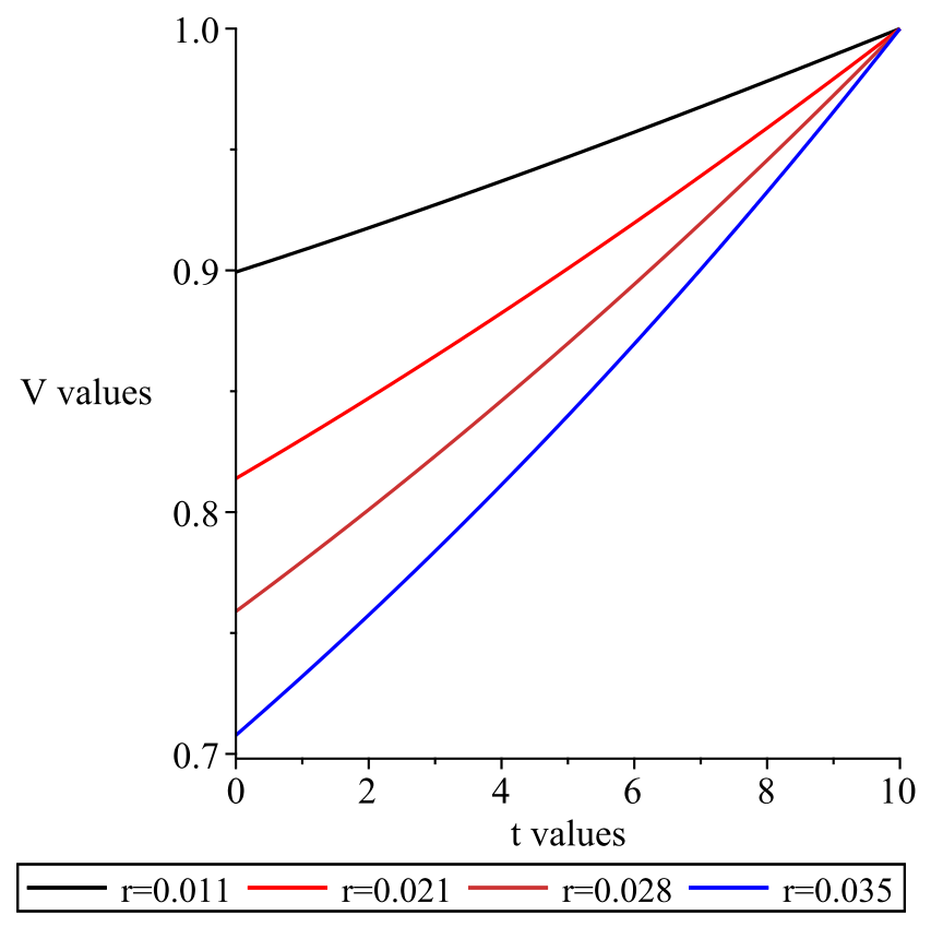
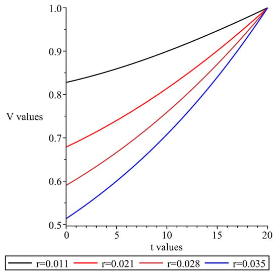
We note that when or , then as given in (40) tends to the value given in (33). In Figure 5 and Figure 6, we plot which when corresponds to the first approximation for . As expected, as the rate r increases, the corresponding bond price becomes less valuable.
Figure 5.
Plot of for various r values with , , , , , , .
Figure 6.
Plot of for various r values with , , , , , , and .
3.2. The Term
We now consider the approximation in (31).
Substituting (31) into (30) and collecting the coefficients of , we obtain that needs to satisfy
subject to
In the case or , we obtain from solving (41) that
For or , solving (41) by the method of characteristics, we obtain
where with replaced by (and so is replaced by ) with A constant,
and
After integration, we replace A with The function is chosen so that
Letting the integral expression in (42) be denoted by Q, we have
After some simplification, we obtain
where and are given in Appendix D.
For the function , we obtain that
for ,
where
and for ,
where
We note that this solution for in the limit is consistent with the solution of stated earlier in the same limit.
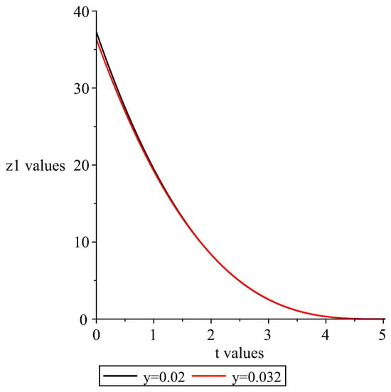
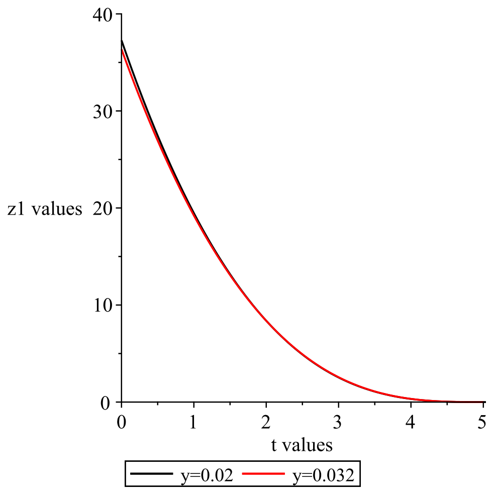
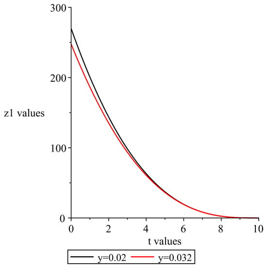
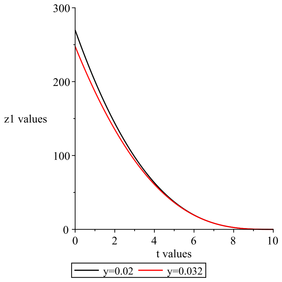
Plots of are given in Figure 7 and Figure 8 with parameters , , and y values 0.02 and 0.032. The plots show little difference between the different y curves except for times very far from expiry.
Figure 7.
Plot of for various y values with , , , , , and .
Figure 8.
Plot of for various y values with , , , , , and .
This leads us to the following result.
Result 2: The price of a zero-coupon bond with principal and expiry time T under the model (28) with is well approximated by
where
with given in (40) and
with Q as in (45) with expressions as in Appendix D, as in (46)–(51), as in (43), and where .
Note that when or , then and .
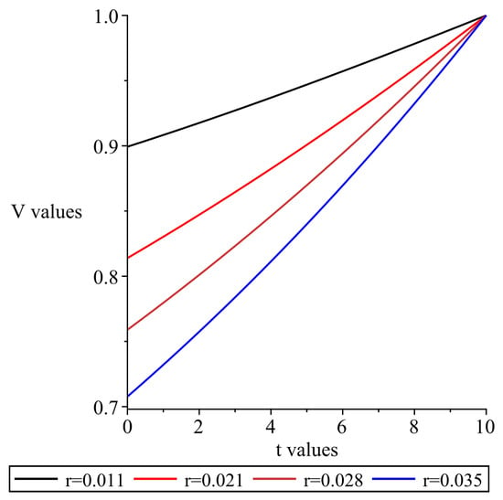
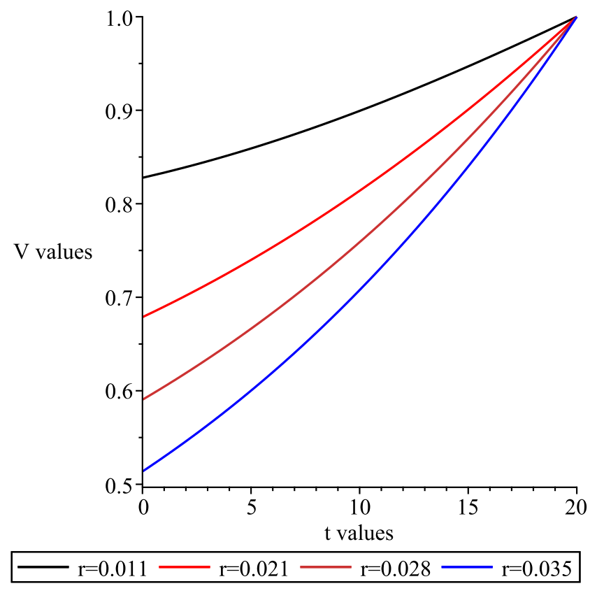
Plots of the solution V as given in Result 2 are shown in Figure 9 and Figure 10 with the parameters As is very small, the contribution of is very minimal and the graphs resemble the ones in Figure 5 and Figure 6 when only is used in the solution. This would typically be the case as a and are very small parameters in the model.
Figure 9.
Plot of (for various r values with , , , , , , and ).
Figure 10.
Plot of (for various r values with , , , , , , and ).
More explicitly, in Table 1, for the parameters as in Figure 7 and Figure 8, we provide the ratios of the second term to the first term and see that they are significantly smaller than one. This means we have a well-behaved expansion.
Table 1.
Sizes of perturbation expansion terms in Equation (31) with , , , , .
Accuracy
To test the accuracy and validate our solution, we compare our results with that obtained numerically on Equation (29). For the numerical scheme, we used the Crank–Nicolson method, which is a second-order accurate finite difference scheme that averages the explicit and implicit Euler methods. It is unconditionally stable (see Wilmott [19]). We used the increments in and r as , respectively. The results are listed in Table 2. From the table, we see that our analytic approximation in Result 2 is highly accurate with absolute errors (AE) of 0 when and at most when .
Table 2.
Comparison of results using the analytic approximation V as in Result 2 () with the numerical Crank–Nicolson scheme () with , , , , . AE represents the number of absolute errors.
3.3. Yield Curve Under the Bimodal Model
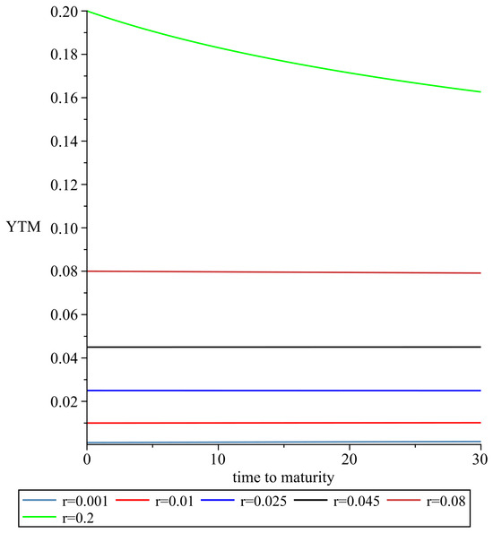
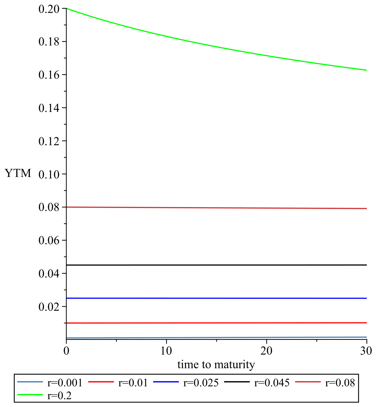
The yield curve (see [19,20]) is a measure of future values of interest rates. Using V as in Result 2, the yield curve is plotted in Figure 11 with parameter values as given in the caption. For interest rates within and near the two modes, the yield curve is essentially flat. This result is a plausible outcome in a bimodal nonlinear short-rate model when the dynamics are strongly mean-reverting (as it is here) toward two stable regions. Intuitively, if the current short rate lies in the low-probability transition zone between the two modes, the market may anticipate movement toward one of the stable states relatively quickly. In that case, bond prices—and thus yields as well—are driven less by the instantaneous rate itself and more by the expected future distribution of rates. When the two modes exert roughly balanced influence in that intermediate region, the expected path of future rates may not vary much, as the current rate moves slightly within the gap between modes. That naturally produces a relatively insensitive or flat response of the yield curve to changes in the current short rate. This is an interesting feature of the model, as it distinguishes it from standard affine models, which typically respond monotonically and smoothly to the current short rate. Flat yield curves can signal uncertainty in the economy and suggest that investors see similar risks both in the short and long term. It normally does not convey the same level of confidence in the market as an upward-sloping curve. It has occurred many times in the past, including in 1994–1995 (US Treasury market) after very aggressive interest rate increases by the Federal Reserve, and more recently in 2022–2024 when many central banks rapidly raised rates to fight inflation.
Figure 11.
Plot of yield curves for various r values with , , , , , and .
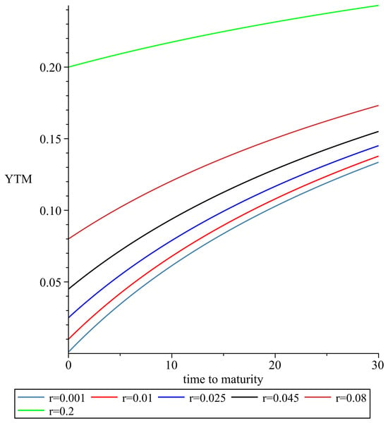
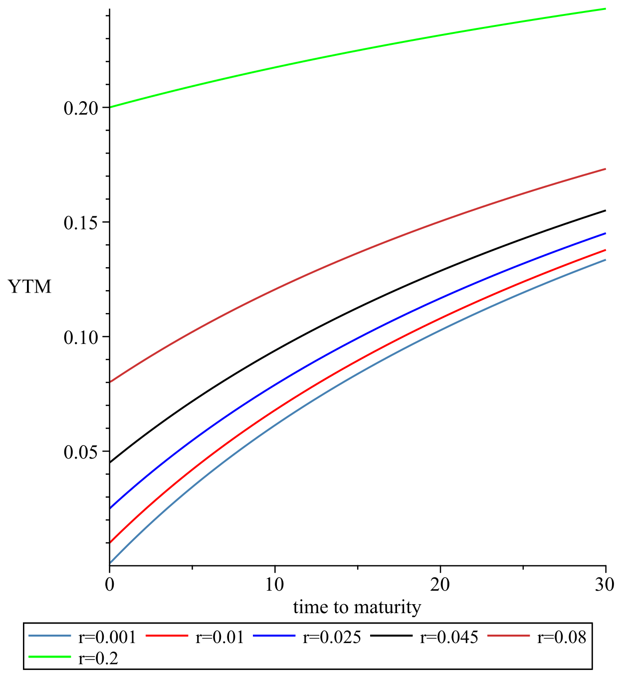
In Figure 12 with , the dynamics are only weakly mean reverting and the yield curves are now monotonically increasing, suggesting that future rates are expected to be higher than the current short-term rate.
Figure 12.
Plot of yield curves for various r values with , , , , , and .
3.4. Calibration
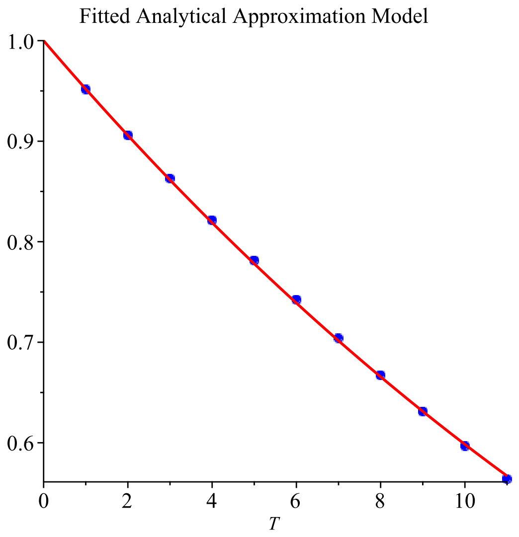
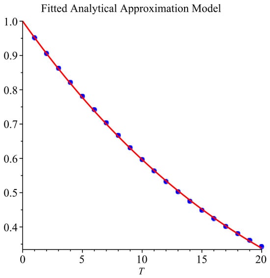
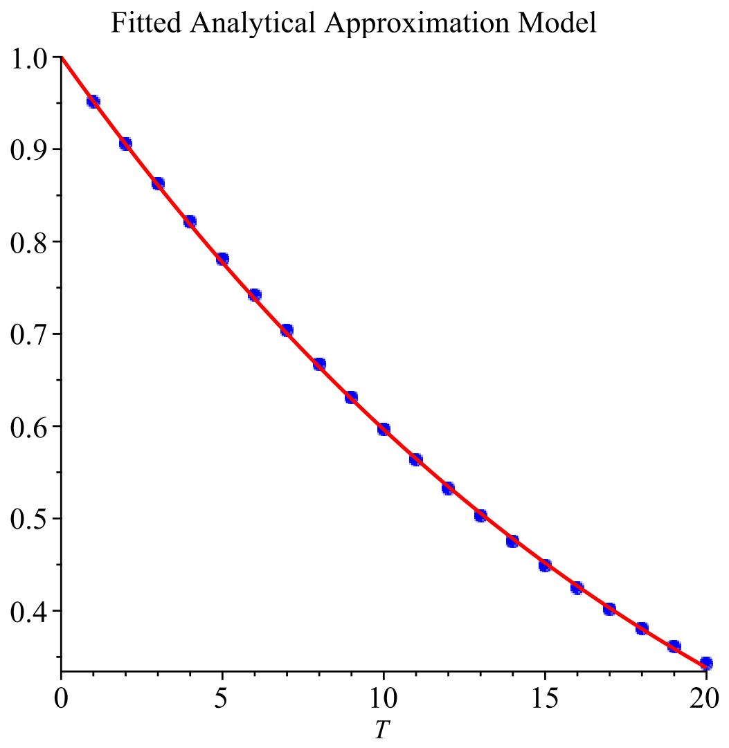
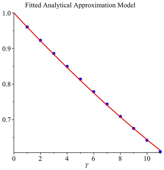
We now fit our solution as in Result 2 using (a) and (b) to data provided by the Federal Reserve’s Gurkaynak–Sack–Wright (GSW) zero-coupon yield estimates [21] with all maturities from 1 to 20 years consecutively for
A1. 9 May 2006 and
A2. 26 June 2026.
To accomplish this, we used the Mathematics package Maple [22] and its optimisation function NonlinearFit as well as the Direct Search package. The NonlinearFit command fits a model nonlinear function in the model parameters to data by minimising the least-squares error. The Direct Search package, however, is designed to numerically compute local and global minimums and maximums for nonlinear multivariate functions without requiring gradient information. This was useful for the full solution in Result 2.
We also fit the models to shorter datasets. Our shorter datasets are with maturities up to 11 years (11 data points), which we call (20xx, short). The longer datasets (20xx, long) have 20 data points.
For comparison purposes, we also fit the datasets to the popular Vasicek [1] and CIR models [2]. The Vasicek model is based on the risk-neutral model and the CIR on . Please see Wilmott [19] for the bond price solutions.
Tabulated in Table 3 are the results of Err = for each fitting as well as the parameters for the best-fit models.
Table 3.
Errors in calibrating market and model prices .
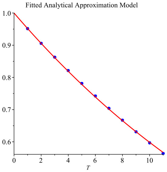
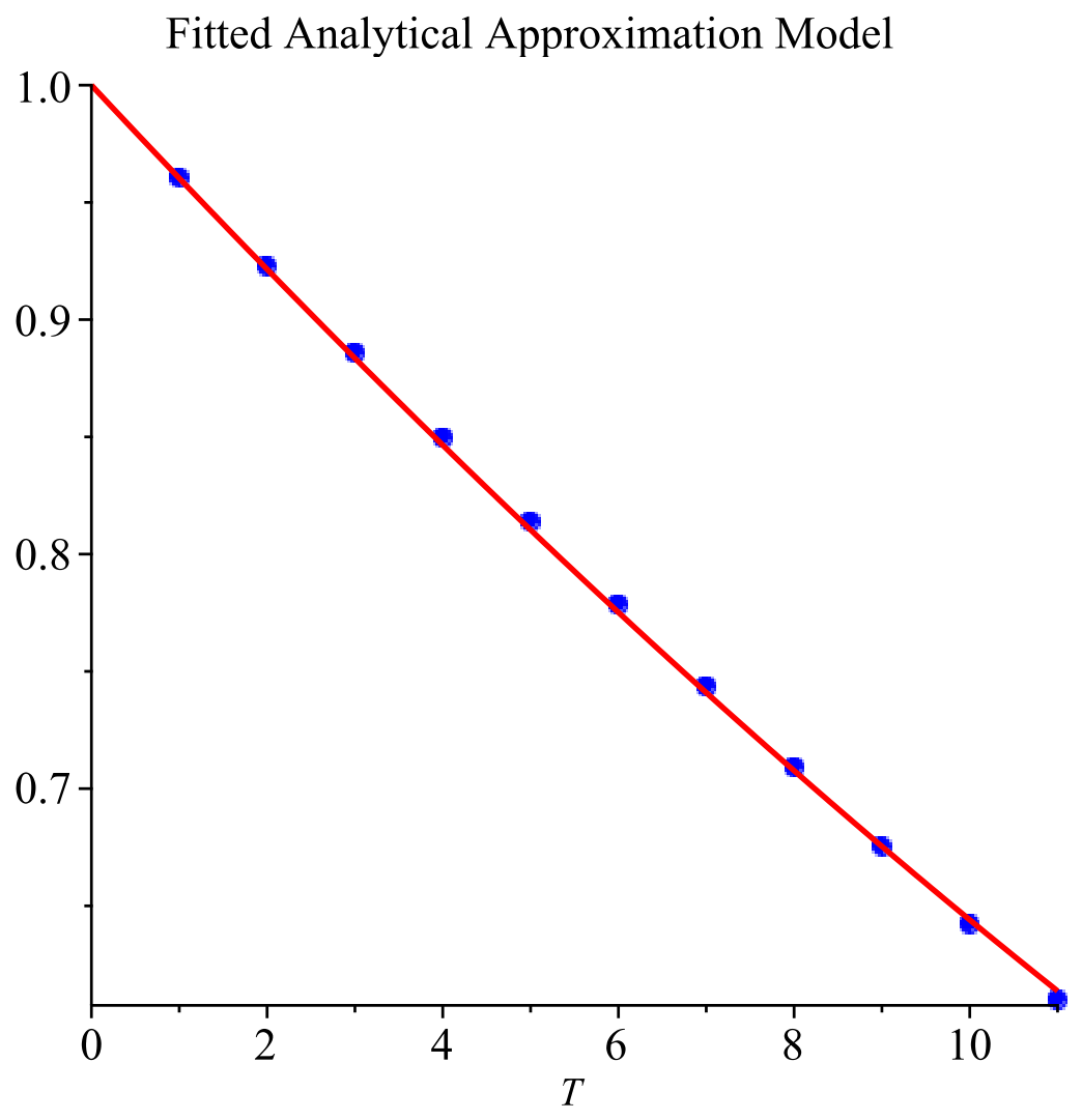
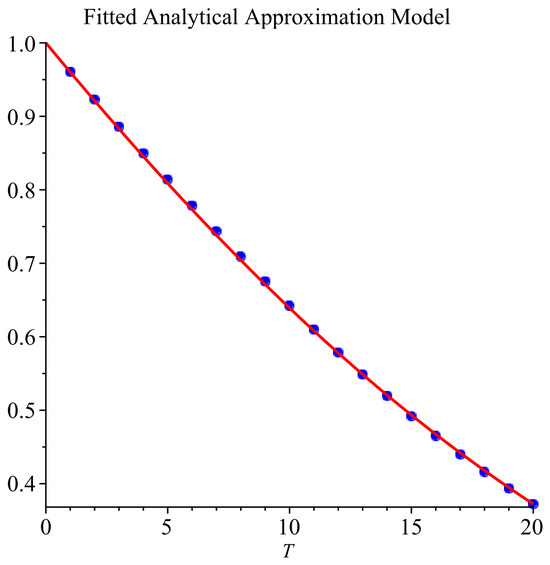
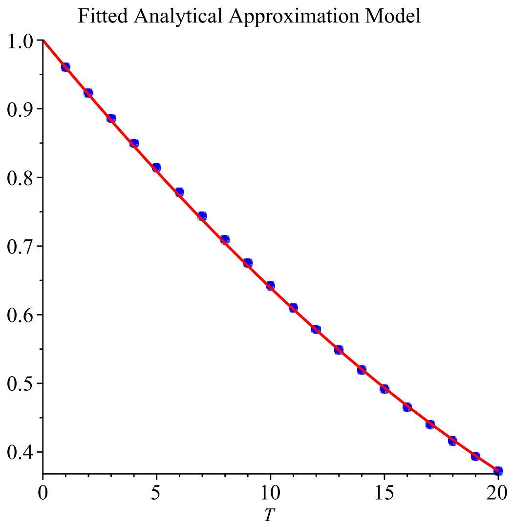
From Table 3, we see that for all datasets, our solution using Result 2 () was an excellent fit to the data, outperforming the Vasicek and CIR models. As expected, though, the first-order approximation solution of Result 2, , was the clear best performer, reducing the error of the zeroth-order approximation solution by up to 84%. The close fit of our simple solution to the datasets in 2006 can be seen in Figure 13 and Figure 14, while its close fit to the datasets in 2026 can be seen in Figure 15 and Figure 16.
Figure 13.
Plot of calibration results using the zeroth-order approximation of Result 2 with the (2006, short) data.
Figure 14.
Plot of calibration results using the zeroth-order approximation of Result 2 with the (2006, long) data.
Figure 15.
Plot of calibration results using the zeroth-order approximation of Result 2 with the (2026, short) data.
Figure 16.
Plot of calibration results using the zeroth order approximation of Result 2 with the (2026, long) data.
In Table 4, using the calibrated sets from Table 3 for Result 2, , we list the perturbation parameter, , and for , the ratio of the first-order correction term to the base term, , and approximation errors relative to the numerical solution using the Crank–Nicolson method, . The results demonstrate again that our analytic approximation in Result 2 is very well behaved and is highly accurate for all the datasets. The parameters , , and are also listed. They characterise the equilibria of the risk-neutral short-rate dynamics and therefore should not necessarily be interpreted as the corresponding physical measure equilibria (In particular, the calibrated negative values of do not imply that the historical short rates have a negative long-run equilibrium. It reflects the risk-neutral dynamics required to reproduce the observed term structures).
Table 4.
Results using Result 2, solutions from Table 3 with the calibrated parameters.
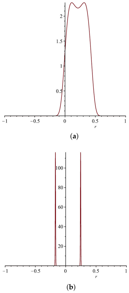
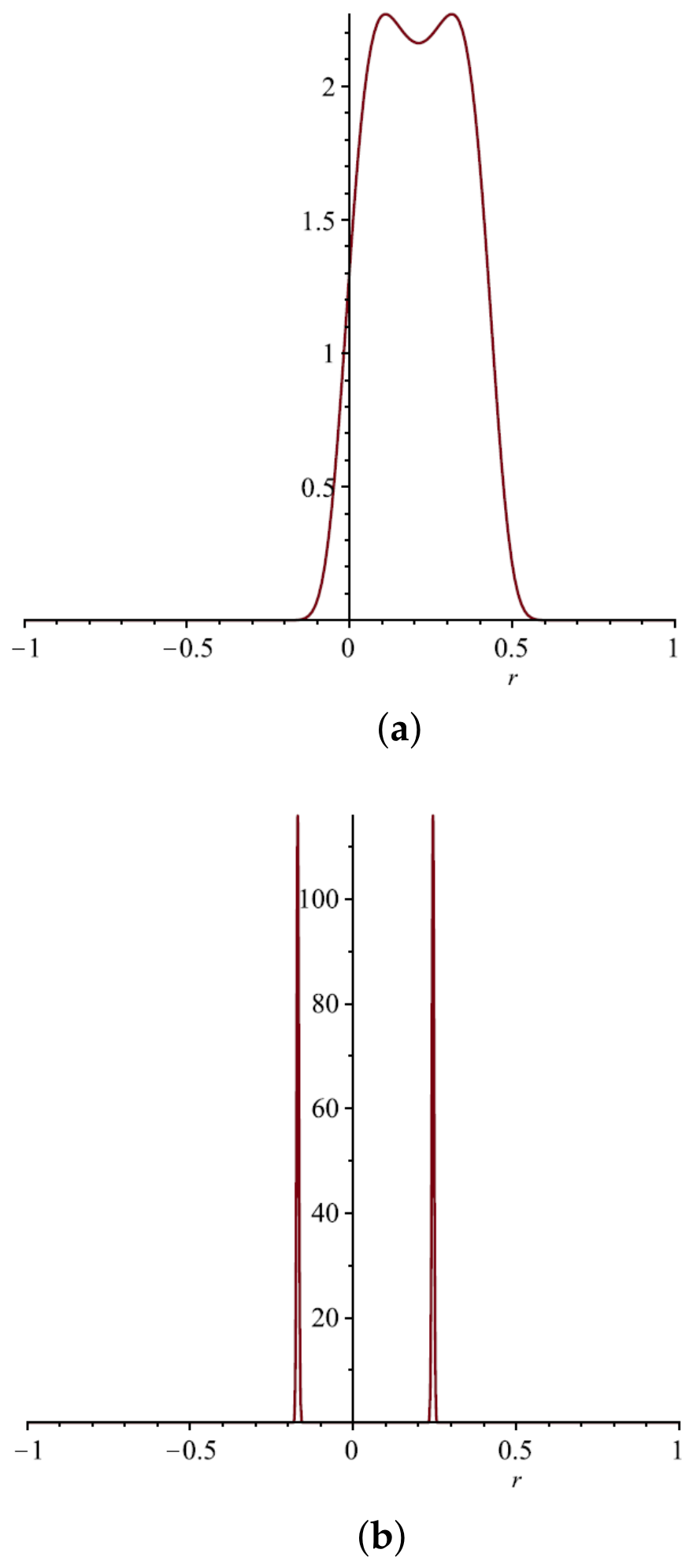
We now come to the last column in Table 4. In Appendix E, we formulate the model-implied stationary density for (27). Plots of the densities with the calibrated values for the (2006, long) and (2026, long) datasets are provided in Figure 17a,b.
Figure 17.
Plot of stationary density (a) using (2006, long) calibrated values and (b) using (2026, long) calibrated values.
From the plots, we see how the three roots and determine the density’s shape. The stationary density has a bimodal shape with probability concentrated around and separated by a low-density region around . In fact, if we write the stationary density as
where
we see that its exponent contains . Hence, for equally spaced roots, taking , then is a natural dimensionless parameter controlling how strongly the stationary density separates into two modes. It has an important effect on the density: increasing it will make the density concentrate more strongly around the stable equilibria. As becomes larger, the exponential increasingly magnifies the difference between the maxima (at and ) and the surrounding values. Thus, the density becomes increasingly concentrated around and . In the limit as , the stationary distribution approaches two increasingly narrow peaks around the stable equilibria. On the other hand, as , the exponential becomes flatter, so the density becomes more spread out.
Hence, gives a natural measure of the strength of bimodality/concentration. In Table 4, we provide the values of using the calibrated values for each of the datasets. These values are large for three of the four datasets, so that the corresponding densities will be very concentrated around the and values. From Figure 17a,b, as expected, the (2026, long) density with is very peaked and the (2006, long) density with is weakly bimodal with two closely spaced local maxima separated by a shallow central minima.
4. Limitations and Potential Considerations
Symmetric restrictions
The equal-spacing restriction of the fixed points and in our Result 2 is motivated economically by interpreting and as two alternative stable interest-rate regimes and as the transition threshold separating these regimes. Setting imposes symmetry between the two regimes: deviations from the transition threshold towards either regime are measured on the same scale. In the absence of a priori evidence that the transition threshold should be systematically closer to either the higher- or lower-rate regime, equal spacing provides a parsimonious and neutral benchmark specification.
This restriction is not intended to imply that economic interest-rate dynamics are necessarily symmetric. Rather, it provides a tractable benchmark for studying bond pricing under a bimodal short-rate distribution. Furthermore, our calibrations are performed subject to this restriction and show that we can obtain very accurate fittings when calibrating to real data.
Our perturbation solution is accurate for the restricted model; it is not intended as an approximation to the unrestricted assymmetric model.
Parameter stability and identifiability
Further work related to this paper could include the following:
1. A comprehensive analysis of parameter stability and global parameter identifiability. This would require a substantially broader empirical and statistical investigation, including estimations over different samples and/or parameter regions.
2. Establishing whether qualitative properties of the model or the perturbation approximation persist throughout the entire parameter space. In this paper, the relevant requirement for the pricing application is that the approximation remains well behaved and accurate in the parameter region associated with the calibrated model. The numerical comparisons and calibration results provide evidence for this.
5. Conclusions
This paper developed a single-factor nonlinear stochastic interest-rate model capable of generating bimodal behaviour without relying explicitly on a regime-switching framework. As opposed to traditional regime-switching models, where dynamics are driven by latent Markov states and discrete transitions between regimes, the proposed model embeds bimodality directly into the continuous dynamics of the short rate. As a result, the model is able to reproduce heterogeneous interest-rate environments while keeping a unified and consistent stochastic structure.
Within this structure, an analytic approximation for the solution of zero-coupon bonds was derived under the assumption of equidistant fixed points. The approximations were shown to be very accurate when compared to the more computationally intensive numerical solution. Hence, we have demonstrated that tractability can be preserved even in the presence of a very nonlinear drift. This represents an important contribution, as models capable of capturing multiple market equilibria are often associated with significant complexity. The formula we have derived for the bond only involves sums of standard functions and is easily implemented in mathematical computer packages. Unlike many numerical solutions, our explicit solution enables fast and efficient computations and can be calibrated to real data. In this paper, we calibrated our solution to two sets of real-world data, obtaining excellent fits in both cases.
The results provide a foundation for incorporating richer distributional features and offer practical insights for risk management in environments where rates are anchored around multiple equilibria.
The bimodal model provides a natural interpretation of interest-rate dynamics in markets where rates exhibit clustering around distinct levels without abrupt externally imposed regime changes. By avoiding discrete switching mechanisms, the framework reduces dependence on latent state estimation and offers a more straightforward representation of nonlinear term structure behaviour. At the same time, the bimodal structure allows the model to capture features that are difficult to reproduce under standard affine or Gaussian specifications. An interesting implication of the model is that the yield curve may exhibit limited sensitivity to the current short rate when the process lies between the two dominant modes. This occurs because intermediate rate levels are dynamically unstable relative to the attracting regions associated with each mode, causing bond prices to depend primarily on the expected transition toward the stable states rather than on the instantaneous rate itself.
Author Contributions
Conceptualization, J.G. and M.A.; Methodology, J.G. and M.A.; Software, J.G. and M.A.; Validation, J.G. and M.A.; Formal analysis, J.G. and M.A.; Investigation, J.G. and M.A.; Resources, J.G. and M.A.; Data curation, J.G. and M.A.; Writing—original draft, J.G. and M.A.; Writing—review & editing, J.G. and M.A.; Visualization, J.G. and M.A.; Supervision, J.G.; Project administration, J.G. and M.A. All authors have read and agreed to the published version of the manuscript.
Funding
This research received no external funding.
Institutional Review Board Statement
Not applicable.
Informed Consent Statement
Not applicable.
Data Availability Statement
The datasets used in this paper are publicly available through Federal Reserve Economic Data|FRED|St. Louis Fed and https://www.bnm.gov.my/islamic-interbank-rates (accessed on 6 September 2026).
Conflicts of Interest
The authors declare no conflicts of interest.
Correction Statement
This article has been republished with a minor correction to the Appendix E. This change does not affect the scientific content of the article.
Appendix A
In this appendix, we analyse three interest rate datasets for the presence of unimodality or bimodality. These are summarised in the following table.
Table A1.
Interest rate datasets examined for unimodality and bimodality.
Plots and histograms of the data are provided in Figure A1, Figure A2 and Figure A3. We note that in our examination for unimodality or bimodality, no single statistic should be considered in isolation. Rather, for each of the datasets, we believe that the collective evidence from various statistics provides strong justification for adopting bimodal models.
1. Based on Histograms with Kernel Density Overlays
For each dataset, the histograms with kernel density overlays show two clear peaks. These two peaks suggest that the data are grouped around two different values rather than one. The kernel density curves exhibit the same two peaks, confirming that the observed bimodal patterns are not simply artefacts of the histogram representations. Furthermore, the pronounced troughs between the two peaks indicate clear separations between the two groups. Hence, the visual evidence strongly supports the assumption that the data follow bimodal distributions.
2. Based on Hartigan’s Dip Test
Hartigan’s Dip Test [23] is used to check whether a dataset has only one peak. It compares the data with a unimodal distribution. A small p-value suggests that the data are not unimodal and may contain two or more peaks.
For all our datasets, Hartigan’s Dip Test rejects unimodality (with ), indicating a statistically detectable higher-order structure.
3. Based on Silverman’s Test
Silverman’s test [24] is a formal statistical test used to determine the number of modes (peaks) in a distribution. It uses a kernel density estimate to test whether the data contain more than a specified number of modes. A small p-value provides evidence against the null hypothesis, indicating that the data have more modes than specified. The critical bandwidth provided by the test is the smallest kernel bandwidth that makes the estimated density have a specified number of modes (or fewer). The critical bandwidth for k modes, , is the minimum amount of smoothing needed so that the density has at most k modes. Hence, the critical bandwidth for one mode, , is the smallest bandwidth that makes the density unimodal. The critical bandwidth for two modes, , is the smallest bandwidth that makes the density have no more than two modes. However, especially with very large datasets, as we have here, Silverman’s test can detect subtle departures from bimodality—small shoulders or minor peaks that may have little practical importance. The bandwidth sequence, though, can show that the first two modes are the dominant structural features.
For our datasets, Silverman’s test rejects both unimodality and bimodality ( and , respectively), indicating a statistically detectable higher-order structure. However, the critical bandwidths required to reduce the densities to two modes are substantially smaller than those required for unimodality. This suggests that the additional modes are relatively minor compared with the two dominant modes observed in the empirical distribution.
In particular, our IIBR, SOFR and SONIA datasets require large critical bandwidths, namely 0.43854, 1.7268, and 1.9429, respectively, before becoming unimodal, so that each dataset is not truly unimodal. Small p-values mean we reject unimodality.
Much less smoothing (0.10069, 0.434, 0.40742) is required before the densities have only two modes. In fact, it is (4.355, 3.98, 4.768) times smaller. This suggests that any modes beyond the first two disappear quickly with a relatively small amount of smoothing. The fact that is much larger than is consistent with a situation where two dominant modes are separated, while any additional modes are relatively minor fluctuations or local bumps. This is consistent with the interpretation that bimodality is a robust feature of the data and higher order multi-modality may be due to weaker features or sampling variability.
In summary, the results indicate that the main structure of each of our datasets is bimodal. The histograms and kernel density estimates clearly display two dominant peaks separated by a distinct valley. Hartigan’s Dip Test provides strong evidence against unimodality, while Silverman’s test shows that the additional modes detected are relatively small and become apparent only because of the large sample sizes. Since the critical bandwidths required to reduce the densities to two modes are much smaller than those required to obtain unimodal densities, the two dominant modes represent the primary characteristics of the distributions. Hence, for each of the datasets, a bimodal model provides a reasonable and appropriate description.
Figure A1.
(a) Daily SOFR rates, (b) histogram of the daily SOFR rates and (c) histogram with an overlaid kernel density curve.
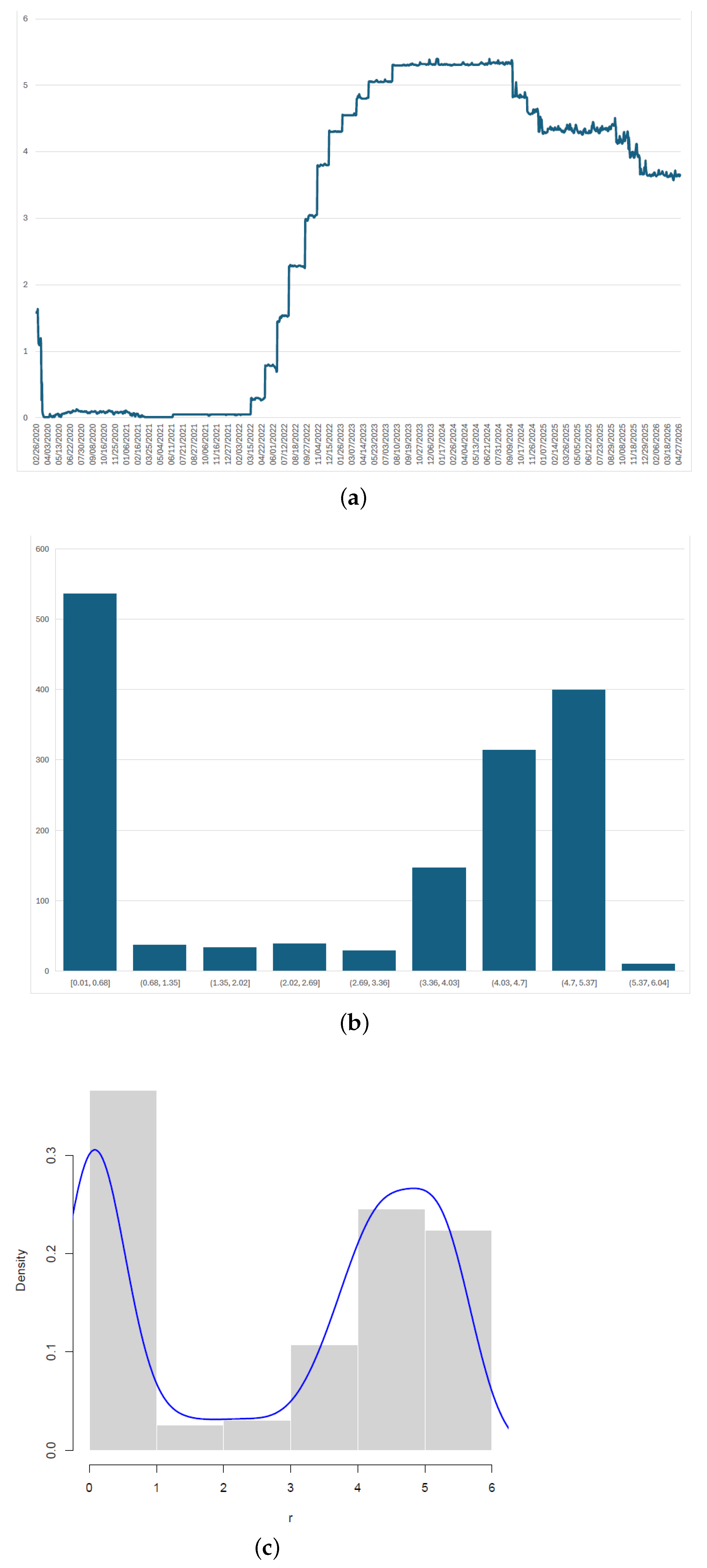
Figure A2.
(a) Daily SONIA rates, (b) histogram of the daily SONIA rates and (c) histogram with an overlaid kernel density curve.
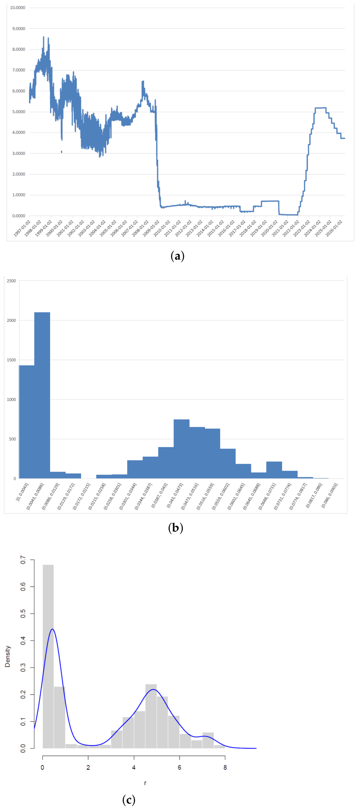
Figure A3.
(a) Daily IIBR rates, (b) histogram of the daily IIBR rates and (c) histogram with an overlaid kernel density curve.
Appendix B
In this Appendix, we derive a system of coupled equations for the value of the bond as given in Section 2, where the interest rate is assumed to have two states . In particular, represents the state when the interest rate reverts to , while represents the state when the interest rate reverts to . Hence, when , then , and the change in the real interest rate is assumed to follow
We assume that the transition between states includes the following movements:
- Jumps from to and occurs as a Poisson process with rate ;
- Jumps from to and occurs as a Poisson process with rate .
Hence, the value of a bond contract will take one of two values or depending on the current state respectively.
Suppose that at time t, , so the value of a bond contract is . In a short time step , the value of the bond contract is given by
Hence, the change in the bond contract can be written as
This is equivalent to
We construct a portfolio with value that consists of one long postilion in a bond contract with expiry and value as well as short positions in bond contracts with expiry and each with value so . The change in our portfolio can be written as
The change in bond prices, , can be found by applying Itôs Lemma, so can be written as
where
The expected value of the change in our portfolio is given by
With the judicious choice of , the risk in our portfolio is eliminated, and the change in the value can be simplified to
Since the portfolio is instantaneously riskless, it must earn the riskless short interest rate; that is, and (A9) can be rewritten as
The left and right-hand sides in Equation (A10) are functions of and , respectively. This means that both sides must be independent of the expiry date. Hence, we can drop the accents and write
for some arbitrary function . We can write as this way represents the market price of risk. Then, on re-arranging (A11), we obtain
We assume the market price of risk is such that the risk-neutral process for r is of the same form as the real process (A1). Hence, we assume , where are constants, and that the risk-free process for r is
where is a Wiener process under which the discounted traded asset prices are martingales.
Hence, we arrive at
which needs to be solved subject to .
- Similarly, if we start with state 2, we obtain
- Letting , we arrive at
Appendix C
In this Appendix, we derive the bond-pricing equation as in Section 3, i.e.,
where and where the real interest rate is modelled by
where and are constant. We begin by setting up a portfolio containing two types of bonds: one with value with maturity and the other with value with a different maturity . We hold one with value and a quantity of the one with value . Hence, the value of the portfolio is
By choosing
then the change in our portfolio in a time can be found to be
Since the portfolio is riskless over an interval , the absence of arbitrage requires its instantaneous return to equal the risk-free rate so that and so
Then, by rearranging the equation with terms on one side and terms on the other, we obtain that
As the only way this is possible is for both sides to be independent of maturity date, we can drop the subscript from V so that
for some function We can write , as this way represents the market price of risk.
Choosing a market price of risk usually involves assuming a particular form for it. Similar to many authors such as [25,26], we assume the market price of risk is such that the risk-neutral process for r is of the same form as the real process (A18). Hence, we assume , where a, and are constants, and that the risk-free process for r is
where is a Wiener process under which the discounted traded asset prices are martingales.
Hence, we arrive at
Appendix D
Here, we list the value of the expressions for Q in Equation (44).
Appendix E
In this appendix, we derive the stationary density for model (27).
- The Fokker–Planck equation for the density is
References
- Vasicek, O. An equilibrium characterization of the term structure. J. Financ. Econ. 1977, 5, 177–188. [Google Scholar] [CrossRef] [Scilit]
- Cox, J.; Ingersoll, J.; Ross, S. A theory of the term structure of interest rates. Econometrica 1985, 53, 385–407. [Google Scholar] [CrossRef] [Scilit]
- Duffie, D.; Kan, R. A yield-factor model of interest rates. Math. Financ. 1996, 6, 379–406. [Google Scholar] [CrossRef] [Scilit]
- Goard, J. New solutions to the bond-pricing equation via Lie’s classical method. Math. Comput. Model. 2000, 32, 299–313. [Google Scholar] [CrossRef] [Scilit]
- Jha, A. A sinusoidal Hull–White model for interest rate dynamics: Capturing long-term periodicity in U.S. Treasury yields. arXiv 2025, arXiv:2506.06317. [Google Scholar]
- Samimi, H.; Najafi, A. Bond and Option Prices under Skew Vasicek Model with Transaction Cost. Math. Probl. Eng. 2021, 2021, 9920240. [Google Scholar] [CrossRef] [Scilit]
- Banos, D.; Ortiz-Latorre, S.; Font, O. Change of measure in a Heston–Hawkes stochastic volatility model. Adv. Appl. Probab. 2024, 56, 1370–1399. [Google Scholar] [CrossRef] [Scilit]
- Lee, Y.; Yang, K. Finite difference method for the Hull–White partial differential equations. Mathematics 2020, 8, 1719. [Google Scholar] [CrossRef] [Scilit]
- Falco, A.; Navarro, L.; Vazquez, C. Finite difference methods for Hull–White pricing of interest rate derivatives with dynamically consistent curves. SSRN 2014. [Google Scholar] [CrossRef] [Scilit]
- Ullah, M. Numerical simulation of Heston–Hull–White three-dimensional PDE with high-order FD scheme. Mathematics 2019, 7, 704. [Google Scholar] [CrossRef] [Scilit]
- Fries, C. A short note on the exact stochastic simulation scheme of the Hull–White model and its implementation. SSRN 2016. [Google Scholar] [CrossRef] [Scilit]
- Treepongkaruna, S.; Gray, S. Short-term interest rate models: Valuing interest rate derivatives using a Monte-Carlo approach. Account. Financ. 2003, 43, 231–259. [Google Scholar] [CrossRef] [Scilit]
- Islamic Interbank Benchmark Rate: Pulse of the Islamic Capital Markets. Available online: https://www.sesric.org/imgs/news/image/646-factsheet.pdf (accessed on 2 August 2025).
- Hamilton, J. A new approach to the economic analysis of nonstationary time series and the business cycle. Econometrica 1989, 57, 357–384. [Google Scholar] [CrossRef] [Scilit]
- Ang, A.; Bekaert, G. Regime switches in interest rates. J. Bus. Econ. Stat. 2002, 20, 163–182. [Google Scholar] [CrossRef] [Scilit]
- Siu, T.; Elliott, R. Semi-Markov-modulated exponential-affine bond prices. Quant. Financ. 2025, 25, 1813–1829. [Google Scholar] [CrossRef] [Scilit]
- Shen, Y.; Siu, T. Pricing bond options under a Markovian regime-switching Hull–White model. Econ. Model. 2013, 30, 933–940. [Google Scholar] [CrossRef] [Scilit]
- Polyanin, A. Handbook of Linear Partial Differential Equations for Engineers and Scientists; Chapman &Hall/CRC: Boca Raton, FL, USA, 2002. [Google Scholar]
- Wilmott, P. Derivatives: The Theory and Practice of Financial Engineering; John Wiley & Sons: Chichester, UK, 1998. [Google Scholar]
- Kwok, Y. Mathematical Models of Financial Derivatives; Springer: Singapore, 1998. [Google Scholar]
- Gurkaynak, R.; Sack, B.; Wright, J. The US Treasury yield curve: 1961 to the Present. J. Monet. Econ. 2007, 54, 2291–2304. [Google Scholar] [CrossRef] [Scilit]
- Maple. Maplesoft; A Division of Waterloo Maple Inc.: Waterloo, ON, Canada, 2018. [Google Scholar]
- Hartigan, J.; Hartigan, P. The Dip Test of Unimodality. Ann. Stat. 1985, 13, 70–84. [Google Scholar] [CrossRef] [Scilit]
- Silverman, B. Using Kernel Density Estimates to Investigate Multimodality. J. R. Stat. Soc. Ser. B Methodol. 1981, 43, 97–99. [Google Scholar] [CrossRef] [Scilit]
- Stein, E.; Stein, J. Stock Price Distributions with stochastic volatility: An Analytic approach. Rev. Financ. Stud. 1991, 4, 727–752. [Google Scholar] [CrossRef] [Scilit]
- Grünbichler, A.; Longstaff, F. Valuing futures and options on volatility. J. Bank. Financ. 1996, 20, 985–1001. [Google Scholar] [CrossRef] [Scilit]

Disclaimer/Publisher’s Note: The statements, opinions and data contained in all publications are solely those of the individual author(s) and contributor(s) and not of MDPI and/or the editor(s). MDPI and/or the editor(s) disclaim responsibility for any injury to people or property resulting from any ideas, methods, instructions or products referred to in the content. |
© 2026 by the authors. Licensee MDPI, Basel, Switzerland. This article is an open access article distributed under the terms and conditions of the Creative Commons Attribution (CC BY) license.