Density-Conditioned Intensity–Topology Decoupling in Directed Global Stock-Market Volatility Networks: Effective Transfer Entropy and Path Homology

Abstract

Weighted directed networks can exhibit stronger aggregate interactions without becoming more integrated or topologically richer. Using daily prices for 32 stock indices over 2006–2026, we construct effective transfer entropy (ETE) networks from range-based variance states and recompute GLMY path homology over a directed edge-density filtration. In 88 overlapping 120-common-date windows, total ETE is associated with a higher density required for global weak connectivity and with smaller integrated first- and second-dimensional Betti curves. These are dependence-aware descriptive associations: reduced-overlap estimates are imprecise, and controls for edge concentration and mean variance reduce the connectivity association to approximately zero. Direct coverage measures show that high-intensity windows can distribute weight broadly while their strongest edges reach nodes unevenly. Exact circular-shift tests yield empty 5% BH-FDR backbones, so individual channels are not treated as established. Null-model, rank-stability, coefficient-field, and discretization checks delimit the fixed-density result. A common absolute-weight contrast yields positive rather than negative TETE–Betti associations, showing that the negative baseline relation is specific to the fixed-density filtration. The results distinguish interaction intensity, dispersion, strong-edge coverage, and directed path-homology organization as separate network dimensions.

1. Introduction

The total weight of a directed network does not determine how its edges are organized. The same aggregate interaction can be distributed across a centralized star, modular chains, reciprocal routes, or a graph containing non-boundary path-homology classes. Interaction intensity, coverage by the strongest edges, and higher-order organization induced by directed paths are therefore distinct network properties. This distinction matters in complex systems because architecture can diversify or amplify shocks even when aggregate link strength is similar [1,2,3,4,5].

Global equity markets provide a demanding setting in which to examine this distinction. International dependence rises during periods of stress, but observed co-movement can reflect contagion, common fundamentals, volatility shifts, or non-synchronous trading [6,7,8,9,10]. A large measure of aggregate information flow therefore need not imply that the highest-ranked links cover all markets evenly or form more independent directed path classes.

Existing financial-network methods provide increasingly detailed measurements of spillovers and systemic importance, while transfer entropy (TE) captures nonlinear directional predictive information and topological data analysis summarizes multiscale structure. However, these strands are usually studied separately. Weighted connectedness studies emphasize total spillovers and node roles; financial applications of persistent homology generally use symmetric point clouds or correlation complexes; and the directed path-homology literature remains largely methodological. The unresolved question is whether stronger pairwise information flow is accompanied by stronger integration and richer directed path organization or whether these network dimensions can move independently.

We address three related questions. First, do the four major stress episodes exhibit distinct directed information-flow roles and filtered path-homology curves? Second, how is aggregate information-flow intensity associated with the edge density required for global weak connectivity and with first- and second-dimensional path-homology summaries? Third, do these relationships remain robust to alternative rolling-window specifications, discretization schemes, dependence-aware inference, concentration controls, conventional network diagnostics, alternative filtrations and coefficient fields, and degree-conditioned and weight-location null models?

The contribution is threefold. First, we construct direction-preserving volatility-information networks from a range-based variance proxy and bias-corrected TE; this is an empirical network construction, not a new TE estimator or a structural causal model. Second, we compare weak connectivity, directly measured strong-edge node coverage, conventional directed-network statistics, and GLMY Betti curves over a common rank-based filtration. Third, we document a fixed-density divergence: conditional on retaining the same number of strongest edges, high-TETE windows tend to require denser weak-connectivity coverage and exhibit smaller integrated $H_1$ and $H_2$ dimensions. This pattern reverses under a common absolute-weight filtration and is therefore interpreted as a rank-conditioned structural diagnostic rather than a filtration-invariant law. Concentration and coverage comparisons further distinguish total weight, weight dispersion, node reach, and directed path organization.

2. Literature Review

2.1. International Market Integration, Contagion, and Crisis Transmission

The first strand studies international stock-market integration and contagion. Early evidence documents transmission in returns and volatility across major trading regions [11,12], while extreme-correlation and tail-dependence studies show that diversification benefits can weaken precisely when markets are under stress [6,9]. A central identification issue is whether a post-shock rise in correlation represents contagion or a continuation of pre-existing interdependence under higher volatility [7,8]. Crisis-specific evidence further identifies heterogeneous transmission during the global financial crisis, the European sovereign-debt crisis, COVID-19, and the Russia–Ukraine war [13,14,15,16,17,18,19]. Nonlinear international-market studies, including work published in Mathematics, reinforce that dependence can differ across positive and negative shocks and across economic regimes [20]. This literature motivates our multi-crisis design, while its identification cautions motivate our use of predictive-information rather than causal-contagion language.

2.2. Econometric Connectedness and Complex Financial Networks

The second strand represents financial systems as directed networks. Granger-causality, CoVaR, and variance-decomposition approaches identify systemically important institutions or markets and quantify directional spillovers [21,22,23,24,25]. High-dimensional and frequency-specific extensions allow connectedness to vary across large systems and investment horizons [26,27]. Recent time–frequency and quantile connectedness studies further show that directional roles can be reconfigured across supply-chain shocks, sustainability-linked assets, cryptocurrencies, and fragmented currency-access systems [28,29,30]. Granger-causality networks also demonstrate that market closing-time proximity affects inferred international links [10], which is directly relevant to the uniform-lag limitation of our baseline design. The broader financial-network literature shows that contagion and stability depend on topology, concentration, and balance-sheet or market structure rather than on aggregate exposure alone [2,4,31,32,33].

Recent Mathematics articles extend this strand through sectoral volatility-spillover networks, multiplex recurrence networks, network-induced soft sets, and correlation- or TE-based portfolio networks [34,35,36,37]. These studies demonstrate the value of dynamic and nonlinear network representations, but they primarily evaluate link strengths, centralities, communities, recurrence, or portfolio performance. The present paper instead asks whether aggregate directed information flow and higher-dimensional organization of allowed directed paths provide non-redundant system coordinates.

2.3. Transfer Entropy and Directional Information Flow

The third strand uses information theory to study nonlinear directional dependence. TE measures the information supplied by a source history about a target’s next state beyond the target’s own history [38]. Financial applications range from bilateral market information flow to networks of companies, equity and commodity markets, and global stock indices [39,40,41,42,43]. Effective TE and bootstrap or surrogate procedures are important because plug-in TE is upward biased in finite samples [43,44]. Recent evidence shows that net TE roles can change across COVID-19 and geopolitical stress and across asset classes [45]. Gong et al. [42] are closest to our data construction because they combine the same range-based variance expression with TE-based global stock-market connectedness. We extend that framework by using circular-shift bias correction, multiple-testing diagnostics, a fixed-layout event comparison, and a directed path-homology filtration.

2.4. Topological Data Analysis and Directed Path Homology

The fourth strand applies topology to financial data. Correlation-based networks first established that market structure can be examined across hierarchical scales [46,47]. Persistent-homology studies subsequently used point clouds, delay embeddings, persistence landscapes, and symmetric complexes to identify crashes, regimes, sectoral differences, and bubbles [48,49,50,51,52]. A recent Mathematics review emphasizes that filtration design determines which notion of scale or importance a topological analysis captures [53]. These methods provide useful multiscale summaries, but their usual symmetric constructions do not preserve sender–receiver asymmetry.

GLMY path homology acts directly on allowed paths in a directed graph [54]. Persistent path homology supplies a barcode framework for weighted digraphs [55], and motif and temporal-network applications show that path homology distinguishes directed organizations that conventional graph summaries may merge [56]. The present study does not compute persistence modules or barcodes. It recomputes GLMY homology at nested edge-density levels and therefore uses the precise term multiscale filtered path homology.

Table 1 positions the paper relative to closely related studies. Its marginal contribution is the joint treatment of nonlinear direction, rolling information-flow intensity, nested density thresholds, and higher-dimensional directed path organization in one global equity-market design.

Table 1. Positioning of the present study relative to closely related literature.

Study	Empirical Scope	Core Method	Directed	Nonlinear	Dynamic	Directed PH
Diebold and Yilmaz [23]	Financial firms	VAR variance-decomposition network	Yes	No	Yes	No
Výrost et al. [10]	20 developed stock markets	Granger-causality network with timing alignment	Yes	No	Yes	No
Dimpfl and Peter [43]	Credit and risk markets	Effective TE with bootstrap inference	Yes	Yes	Regime	No
Gong et al. [42]	Global stock indices	Range variance and rolling TE network	Yes	Yes	Yes	No
Su and Liu [36]	Chinese stock sectors	Generalized VAR spillover network	Yes	No	Yes	No
Balci et al. [34]	Borsa Istanbul	Correlation networks and network-induced soft sets	No	Yes	Yes	No
Wang et al. [35]	Carbon, energy, and financial markets	Multiplex recurrence network	No	Yes	Yes	No
Ioannidis et al. [37]	26 DJIA stocks	Pearson and effective-TE portfolio networks	Yes	Yes	Yes	No
Gidea and Katz [48]	US equity-market dynamics	Persistent homology of financial time series	No	Yes	Yes	No
Guo et al. [52]	100 Chinese stocks	Persistence landscapes and correlation networks	No	Yes	Yes	No
Chowdhury and Memoli [55]	Directed-network theory	Persistent path homology	Yes	–	Multiscale	Yes
This paper	32 global stock markets	Range variance, ETE, rolling filtration, and GLMY path homology	Yes	Yes	Yes	Yes

3. Materials and Methods

3.1. Data and Variable Construction

The empirical inputs are vendor-provided daily open, high, low, and close (OHLC) levels from the Wind Financial Terminal (Version 26.5) for 32 broad stock-market indices. The requested study interval is 1 January 2006–30 June 2026; the first available trading date differs by exchange, and the common panel begins on 4 January 2006. The selected indices provide continuous OHLC coverage across Europe, Asia, North America, South America, Oceania, Africa, and the Middle East. They are intended to represent major national markets rather than a market-capitalization-weighted or exhaustive universe.

Index levels are used in the local quotation units supplied by Wind, and no common-currency conversion is applied. A constant change in price units cancels from the within-day log ranges used below, whereas converting an index through a time-varying exchange rate would introduce an additional foreign-exchange component. The source files identify daily OHLC fields but do not provide a common intraday timestamp or a harmonized closing-time convention. We therefore describe them as vendor daily index observations and do not claim that the daily closes are simultaneous across markets.

Before analysis, all files were standardized to one row per market and date with columns date, open, high, low, and close. Dates were parsed and sorted, and observations were checked for duplicates, missing or nonpositive prices, and violations of $H\ge \max (O,C)$ or $L\le \min (O,C)$. None of these core checks failed. No interpolation, forward filling, winsorization, or manual outlier deletion was applied. The Israel file contains 21 later observations in July 2026, but all analytical inputs are restricted to the declared end date of 30 June 2026.

The outer union of the exchange calendars contains 6816 distinct dates. The baseline synchronized panel retains the 1860 dates observed for every market, a retention rate of 27.29%, and covers 4 January 2006–30 June 2026. The four event samples contain 150, 149, 189, and 201 common dates, respectively. A rolling window of 120 common dates spans 399–651 calendar days (median 448.5), demonstrating that the strict intersection is much sparser than a single-market trading calendar. This alignment holds the observation set fixed across every directed pair but sacrifices exchange-specific sessions and can interact with closing-time differences. Pairwise-calendar and time-zone-aware designs are therefore extensions rather than properties established by the baseline.

Table 2 lists the selected markets and their representative indices.

Table 2. Selected countries/regions and representative stock indices.

No.	Country/Region	Stock Index	No.	Country/Region	Stock Index
1	Argentina	MERVAL	17	Japan	TOPIX
2	Australia	ASX 200	18	South Korea	KOSPI
3	Brazil	IBOVESPA	19	Mexico	IPC
4	Canada	TSX	20	Malaysia	KLCI
5	Switzerland	SMI	21	Netherlands	AEX
6	Chile	IPSA	22	New Zealand	NZX 50
7	China	CSI 300	23	Philippines	PSEi
8	Germany	DAX	24	Poland	WIG20
9	Spain	IBEX 35	25	Saudi Arabia	TASI
10	France	CAC 40	26	Sweden	OMXS30
11	United Kingdom	FTSE 100	27	Singapore	STI
12	Hong Kong	HSI	28	Thailand	SET
13	Indonesia	JCI	29	Türkiye	BIST 100
14	Israel	TA-35	30	Taiwan	TAIEX
15	India	NIFTY 50	31	United States	S&P 500
16	Italy	FTSE MIB	32	South Africa	JSEALSI

Table 3 summarizes the event samples and rolling-window construction.

Table 3. Sample construction and effective calendar coverage.

Quantity	Value
Distinct dates in the outer union	6816
Strict 32-market common dates	1860
Strict-common retention rate	27.29%
Global financial crisis common dates	150
European sovereign-debt crisis common dates	149
COVID-19 common dates	189
Russia–Ukraine common dates	201
120-date rolling span, minimum/median/maximum calendar days	399/448.5/651
Negative range-based variance values	0

Following Garman and Klass [57] and the financial-network implementation of Gong et al. [42], daily stock-market variation is constructed from all four OHLC fields. Because the expression is not square-rooted, it is denoted by $v_{i,t}$ and referred to as a range-based variance proxy:

$$\begin{array}{cc}\hfill v_{i,t}=& 0.511{(H_{i,t}-L_{i,t})}^2\hfill \\ \hfill & -0.019\left[(C_{i,t}-O_{i,t})(H_{i,t}+L_{i,t}-2O_{i,t})-2(H_{i,t}-O_{i,t})(L_{i,t}-O_{i,t})\right]\hfill \\ \hfill & -0.383{(C_{i,t}-O_{i,t})}^2,\hfill \end{array}$$

(1)

where $H_{i,t}$, $L_{i,t}$, $O_{i,t}$, and $C_{i,t}$ are logarithms of the daily high, low, opening, and closing index levels. The estimator uses intraday range information and is more informative than a squared close-to-close return when the objective is daily variation. None of the computed values is negative. The baseline uses $v_{i,t}$ directly. As a validation, replacing it by $\sqrt{\max (v_{i,t},0)}$ changes none of the three-state assignments because the square root is monotone and the empirical cut points are transformed consistently.

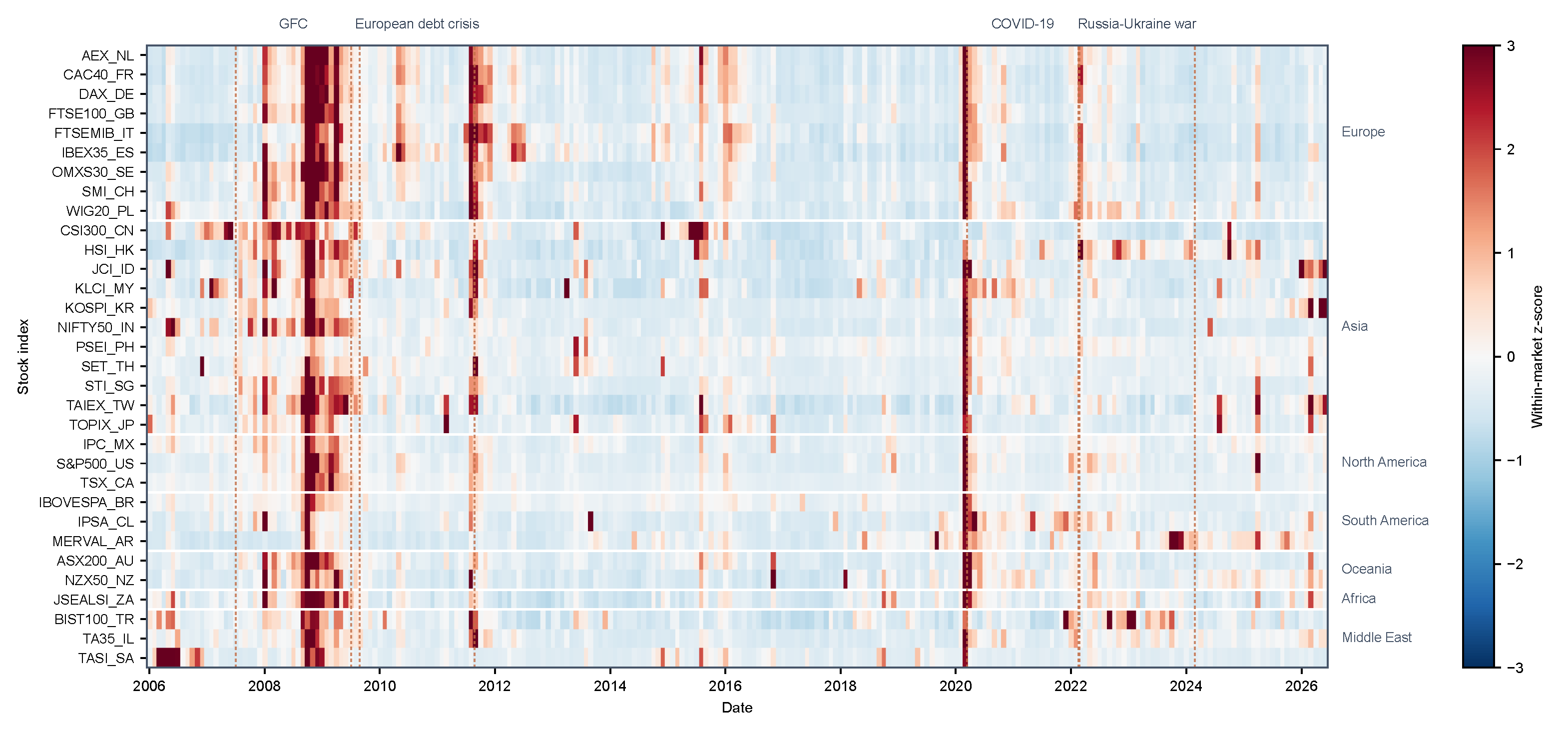
For the monthly standardized-volatility visualization reported in Section 4.2 only, daily values were aggregated to monthly averages and standardized within each market using its full-sample mean and standard deviation. These z-scores are descriptive and do not enter the ETE estimates. All information-theoretic and topological calculations use the unstandardized daily range-based variance proxy.

3.2. Descriptive Statistics and Cross-Market Correlations

Table 4 reports market-level statistics for the synchronized range-based variance panel. Values are multiplied by ${10}^4$ for readability. The series are strongly right-skewed and leptokurtic: means range from 0.283 for Malaysia to 3.143 for Argentina, while rare daily observations generate much larger maxima and positive excess kurtosis in every market. These distributional features support a discrete, nonparametric information-flow approach and caution against interpreting normal-theory correlation as a complete dependence measure [43,44].

Table 4. Descriptive statistics of the range-based variance proxy on the 1860-date strict-common panel. All variance statistics are multiplied by ${10}^4$; kurtosis is excess kurtosis.

Market	N	Mean	SD	Min.	Max.	Skew.	Ex. Kurt.
GB	1860	0.758	1.503	0.022	26.401	7.71	84.72
DE	1860	0.981	1.677	0.010	22.139	6.08	51.14
FR	1860	0.927	1.605	0.027	23.709	6.67	62.71
IT	1860	1.251	2.049	0.000	32.055	7.12	80.04
ES	1860	1.143	1.795	0.037	28.227	6.18	59.34
NL	1860	0.785	1.397	0.022	24.652	7.13	78.97
CH	1860	0.608	1.190	0.033	24.536	9.65	140.61
SE	1860	0.963	1.699	0.019	34.870	7.63	103.89
PL	1860	1.280	2.110	0.030	39.319	8.60	113.89
CN	1860	1.654	3.280	0.032	47.840	6.54	60.47
HK	1860	0.979	1.593	0.000	22.799	6.66	61.35
JP	1860	0.667	2.011	0.014	67.129	22.18	667.97
KR	1860	0.860	2.223	0.037	38.888	9.49	115.56
TW	1860	0.540	0.998	0.015	17.570	9.08	116.76
IN	1860	1.049	3.273	0.019	109.855	21.80	672.00
SG	1860	0.453	1.006	0.019	30.116	16.08	419.29
MY	1860	0.283	0.570	0.005	12.328	10.62	171.57
ID	1860	0.835	1.992	0.000	51.497	12.33	250.25
TH	1860	0.697	3.220	0.020	124.793	32.10	1198.66
PH	1860	0.646	3.200	0.013	133.260	38.47	1589.02
US	1860	0.738	1.611	0.013	30.977	8.49	108.22
CA	1860	0.695	2.250	0.012	66.130	16.98	419.36
MX	1860	0.923	1.849	0.045	43.127	13.22	239.75
BR	1860	1.860	5.671	0.040	137.523	17.16	358.42
CL	1860	0.718	1.796	0.024	39.713	12.87	220.20
AR	1860	3.143	5.976	0.002	148.196	11.70	224.14
AU	1860	0.479	0.981	0.012	22.316	10.82	177.27
NZ	1860	0.294	0.508	0.006	7.759	6.86	63.67
ZA	1860	0.853	1.349	0.021	30.508	9.10	149.73
TR	1860	1.716	2.952	0.039	67.530	9.68	159.63
IL	1860	0.578	1.181	0.013	24.815	10.46	159.00
SA	1860	0.957	2.653	0.000	38.947	7.07	64.52

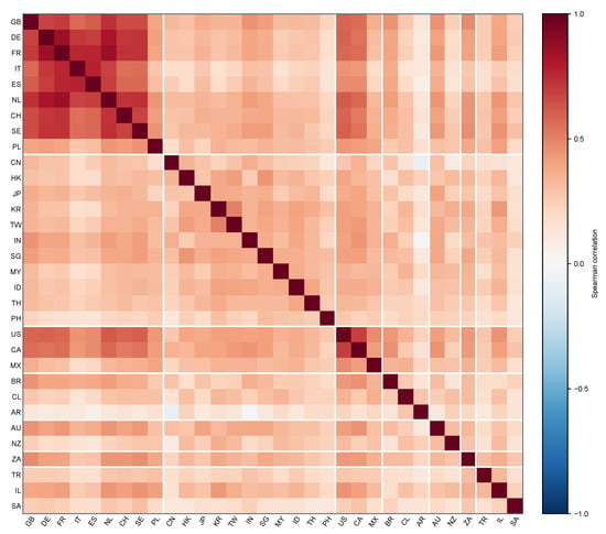
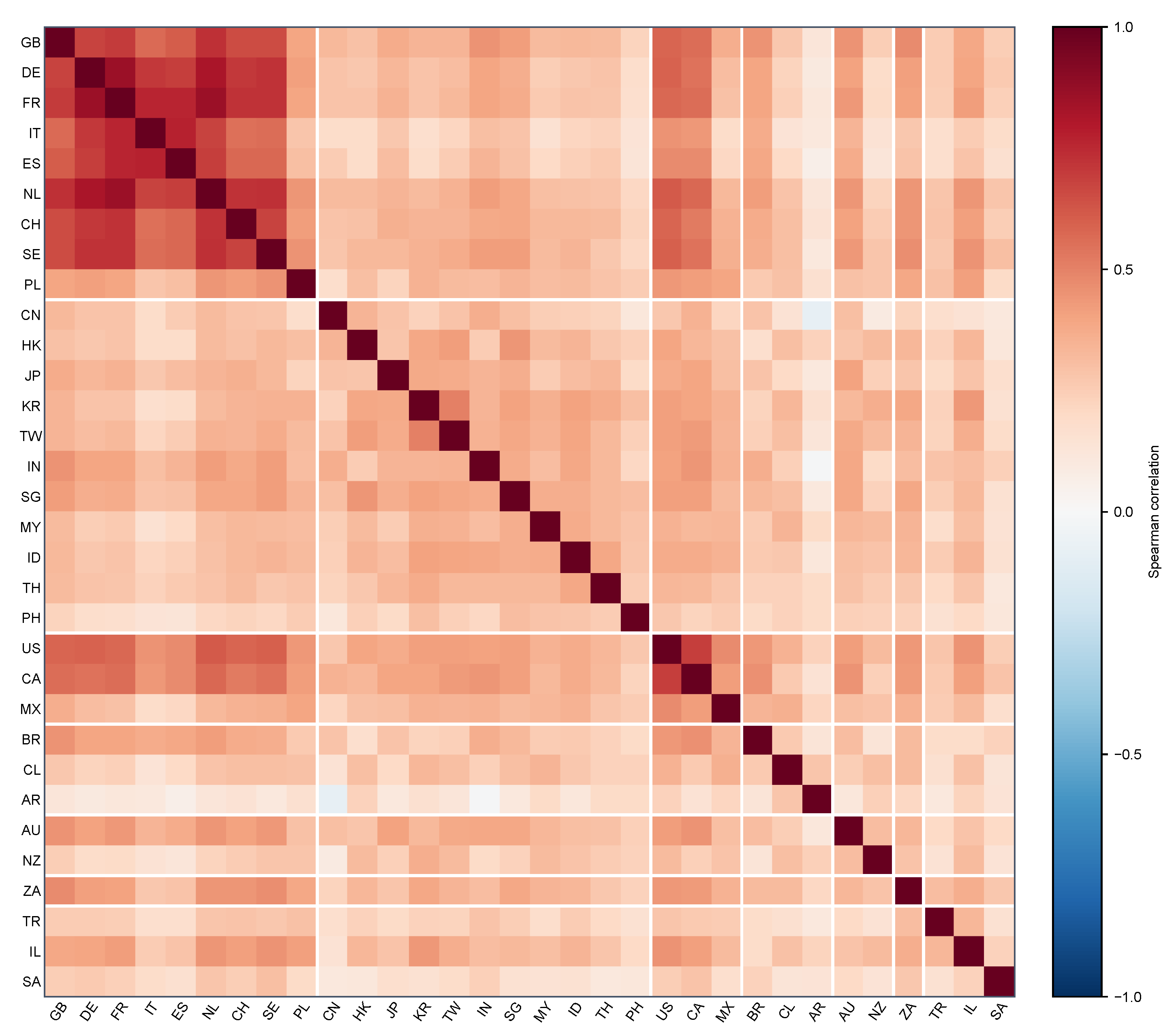
Figure 1 reports pairwise Spearman correlations using the same 1860 dates. The median off-diagonal correlation is 0.307, with an interquartile range of 0.238–0.382. Mean within-region correlation is 0.430, compared with 0.293 across regions; Germany–France is the strongest pair (0.858), whereas China–Argentina is the weakest ($-0.081$). The block structure is consistent with regional integration documented in international-market studies [9,11,12], but the substantial cross-region correlations also show why a purely regional or correlation-only representation is incomplete.

Figure 1. Spearman correlation matrix of the daily range-based variance proxy for 32 stock markets over the 1860 strict-common dates. Markets are ordered by region, and white separators identify regional blocks. The matrix is descriptive and symmetric; the subsequent ETE networks evaluate lagged directional predictive information.

3.3. Information-Theoretic Construction of Directed Volatility Networks

Directional predictive information was quantified using transfer entropy [38]. Let $x_{i,t}$ denote the discretized variance state of target market i and $x_{j,t}$ that of source market j. For history lengths $k=l=1$, TE from j to i is

$$\begin{array}{cc}\hfill T{E}_{j\to i}=& \sum _{x_{i,t+1},x_{i,t},x_{j,t}}p(x_{i,t+1},x_{i,t},x_{j,t}){\log }_2{\displaystyle \frac{p(x_{i,t+1}\mid x_{i,t},x_{j,t})}{p(x_{i,t+1}\mid x_{i,t})}}.\hfill \end{array}$$

(2)

The estimator uses empirical transition frequencies. Terms with zero joint probability contribute zero, and no pseudocount is added. The lag-one specification limits the state-space burden in event samples of 148–200 transitions and follows prior financial TE applications [41]; it captures directional predictive information at the synchronized common-observation lag, not structural causality. Here, t and $t+1$ are consecutive rows of the strict-common panel. Thus, $x_{j,t}$ is never used to predict $x_{i,t}$ on the same calendar date. Nevertheless, the elapsed clock time from $x_{j,t}$ to $x_{i,t+1}$ differs across regional pairs, and adjacent common observations need not be one calendar day apart.

Each market-specific $v_{i,t}$ series was partitioned at its full-sample $1/3$ and $2/3$ quantiles. Holding these thresholds fixed gives comparable state definitions across retrospective windows, but it uses observations that would be unavailable in real time. We therefore also re-estimated the 120-date networks using $1/3$ and $2/3$ cut points calculated separately inside each window. This endpoint-available specification uses no observation after that window, although its state meanings can vary across windows. Four-state discretization provides a further sensitivity check. The baseline remains a retrospective comparison and is not presented as an online early-warning estimator.

Because plug-in TE is upward biased in short samples, the source-state sequence of length T was circularly shifted through every distinct nonzero offset $s=1,\dots ,T-1$, while the target sequence was held fixed. Thus, each possible nonzero circular shift enters exactly once; no repeated random offsets are treated as additional randomization states. Circular shifts disrupt source–target alignment while retaining the source’s state ordering around the circular boundary. The surrogate mean is

$${\overline{TE}}_{j\to i}^{\mathrm{shift}}={\displaystyle \frac{1}{T-1}}{\displaystyle \sum _{s=1}^{T-1}}T{E}_{j\to i}^{\left(s\right)},$$

(3)

and effective transfer entropy was defined as

$$ET{E}_{j\to i}=\max \left\{T{E}_{j\to i}-{\overline{TE}}_{j\to i}^{\mathrm{sur}},0\right\},$$

(4)

where ${\overline{TE}}_{j\to i}^{\mathrm{sur}}={\overline{TE}}_{j\to i}^{\mathrm{shift}}$. Negative bias-corrected values were set to zero. This subtraction is a bias correction and is not itself a significance test.

For inferential diagnostics, a one-sided empirical p value was calculated as

$$p_{j\to i}^{\mathrm{shift}}={\displaystyle \frac{1+{\sum }_{s=1}^{T-1}\mathbf{1}\left(T{E}_{j\to i}^{\left(s\right)}\ge T{E}_{j\to i}^{\mathrm{obs}}\right)}{T}},$$

(5)

where the additional state in the denominator is the unshifted observed sequence. The smallest attainable exact p value is therefore $1/T$. The 992 directed tests were adjusted within each event or rolling window by the Benjamini–Hochberg procedure at 5%. These FDR results are reported separately. The main weighted filtration retains positive bias-corrected ETE values even when they do not pass FDR and is consequently interpreted as descriptive.

All markets use the same retained calendar date and a uniform lag of one common observation. This convention is reproducible but does not align exchange closing times. Circular shifting addresses finite-sample bias and supplies a randomization distribution under this retained alignment; it does not correct exchange-calendar or closing-time asynchrony. Apparent geographic direction, particularly between Asian and Western markets, can therefore reflect unequal clock-time horizons as well as predictive dependence. We use “alignment-dependent predictive-information role” and do not interpret pairwise ETE as a chronological within-session or causal contagion channel. A time-zone-aware lead–lag network and global-factor-residualized ETE are not estimated in this study.

The resulting global volatility-information system was represented as a weighted directed graph

$$G=(V,E,w),$$

(6)

where $V=\{v_1,\dots ,v_N\}$ denotes the set of stock markets, $E\subseteq V\times V$ denotes directed information-transmission relations, and

$$w(v_i,v_j)=ET{E}_{i\to j}$$

(7)

assigns the effective transfer entropy from market i to market j as the corresponding edge weight.

The directional role of each market was characterized by its total outgoing and incoming information flows,

$$T{O}_i=\sum _{j\ne i}ET{E}_{i\to j},FRO{M}_i=\sum _{j\ne i}ET{E}_{j\to i},$$

(8)

with net information transmission given by

$$NE{T}_i=T{O}_i-FRO{M}_i.$$

(9)

A positive $NE{T}_i$ identifies a market whose outgoing information flow exceeds its incoming flow, whereas a negative value identifies a net information receiver. Bilateral asymmetry was further summarized by

$$NetET{E}_{ij}=ET{E}_{i\to j}-ET{E}_{j\to i}.$$

(10)

Net ETE therefore provides the dominant direction of bilateral information transmission, while the original directed ETE matrix preserves both directional components and was retained for subsequent regional and topological analyses.

The information network was examined both over economically meaningful stress periods and through continuous rolling estimation. Four major episodes were considered: the global financial crisis from 2 July 2007 to 2 July 2009, the European sovereign-debt crisis from 25 August 2009 to 25 August 2011, the COVID-19 pandemic from 11 March 2020 to 18 February 2022, and the Russia–Ukraine war from 24 February 2022 to 24 February 2024. The same period definitions were used throughout the event-specific analysis.

To characterize temporal evolution, the directed ETE network was re-estimated in rolling samples of 120 common dates advanced by 20 common dates. Robustness specifications use 180 and 240 common dates and four states. The aggregate intensity at rolling time t was

$$TET{E}_t=\sum _{i\ne j}ET{E}_{i\to j,t}.$$

(11)

To test rather than assume a concentration mechanism, edge shares were defined as

$$s_{ij,t}=ET{E}_{i\to j,t}/TET{E}_t.$$

(12)

They were used to calculate

$$HH{I}_{E,t}=\sum _{i\ne j}{s}_{ij,t}^2,N_{E,t}^{\mathrm{eff}}=HH{I}_{E,t}^{-1}.$$

(13)

We also calculated the shares of TETE in the top 1%, 5%, and 10% of edges, the HHI of node out-strength, and the proportion of positive ETE edges. To separate the mechanical lower bound created by the number $M_t$ of positive edges from dispersion among those edges, we additionally report

$$HH{I}_{E,t}^{\mathrm{norm}}={\displaystyle \frac{HH{I}_{E,t}-1/M_t}{1-1/M_t}}.$$

(14)

Geographical transmission patterns were examined by assigning the markets to Europe, Asia, North America, South America, Oceania, Africa, and the Middle East. For sender region $R_a$ and receiver region $R_b$, regional information transmission was summarized as

$${\overline{ETE}}_{R_a\to R_b}={\displaystyle \frac{1}{N_{ab}}}\sum _{i\in R_a}\underset{j\ne i}{\sum _{j\in R_b}}ET{E}_{i\to j},$$

(15)

where $N_{ab}=|R_a\left|\right|R_b|$ for $a\ne b$ and $N_{aa}=|R_a\left|\right(|R_a|-1)$ within a region. The mean rather than the sum avoids mechanically favoring larger regions. Because Africa contains one market, $N_{AA}=0$ and Africa-to-Africa transmission is undefined rather than zero.

For descriptive event-network visualization, one ForceAtlas2 layout [58] was estimated from mean bilateral Net ETE across the four events and then held fixed across panels. Only the strongest 10% of bilateral Net ETE arrows are displayed, whereas node TO, FROM, and NET use the complete ETE matrix. GLMY calculations use the original directed ETE matrix, not the bilateral Net ETE display.

3.4. GLMY Path Homology of Directed Information Networks

The multiscale organization of the directed volatility-information network was characterized using regular path homology within the Grigor’yan–Lin–Muranov–Yau (GLMY) framework [54]. Because information transmission is intrinsically directional, the GLMY analysis was performed on the original directed ETE network rather than on its bilateral Net ETE representation.

Let $G=(V,E)$ be a directed graph. An elementary p-path is an ordered sequence of $p+1$ vertices,

$$e_{i_0\dots i_p}=(v_{i_0},v_{i_1},\dots ,v_{i_p}).$$

(16)

An elementary path is regular if consecutive vertices are distinct. A regular elementary p-path is allowed in G when every pair of consecutive vertices follows a directed edge,

$$(v_{i_{q-1}},v_{i_q})\in E,q=1,\dots ,p.$$

(17)

Let $A_p\left(G\right)$ denote the vector space over the coefficient field ${\mathbb{F}}_2$ generated by all allowed regular p-paths,

$$A_p\left(G\right)={\mathrm{span}}_{{\mathbb{F}}_2}\left\{e_{i_0\dots i_p}:(v_{i_{q-1}},v_{i_q})\in E\mathrm{for}\mathrm{all}q\right\}.$$

(18)

For an elementary p-path, the boundary operator is defined by

$${\partial }_p{e}_{i_0\dots i_p}={\displaystyle \sum _{q=0}^p}{(-1)}^q{e}_{i_0\dots \widehat{i_q}\dots i_p},$$

(19)

where $\widehat{i_q}$ denotes omission of the q-th vertex. Because the computations are performed over ${\mathbb{F}}_2$, the alternating signs are immaterial numerically, although the standard boundary notation is retained.

For directed path complexes, the boundary of an allowed path need not itself be an allowed path. The ∂-invariant path space is therefore defined as

$${\mathsf{\Omega }}_p\left(G\right)=\left\{u\in A_p\left(G\right):{\partial }_{p}u\in A_{p-1}\left(G\right)\right\}.$$

(20)

Because the present analysis considers homology through dimension two, the relevant part of the resulting chain complex is

$${\mathsf{\Omega }}_3\left(G\right)\stackrel{{\partial }_3}{\to }{\mathsf{\Omega }}_2\left(G\right)\stackrel{{\partial }_2}{\to }{\mathsf{\Omega }}_1\left(G\right)\stackrel{{\partial }_1}{\to }{\mathsf{\Omega }}_0\left(G\right)⟶0.$$

(21)

The p-dimensional path-homology group is then defined as

$$H_p\left(G\right)={\displaystyle \frac{\ker \left({\partial }_p{|}_{{\mathsf{\Omega }}_p}\right)}{\mathrm{im}\left({\partial }_{p+1}{|}_{{\mathsf{\Omega }}_{p+1}}\right)}},p=0,1,2,$$

(22)

and the corresponding Betti number is

$${\beta }_p\left(G\right)={\dim }_{{\mathbb{F}}_2}{H}_p\left(G\right).$$

(23)

The zeroth Betti number ${\beta }_0$ is the number of weakly connected components. The first Betti number ${\beta }_1$ is the dimension of the space of non-boundary one-dimensional path-homology classes; it is not a count of simple graph cycles. Likewise, ${\beta }_2$ is the dimension of two-dimensional path-homology classes induced by allowed directed paths, not a count of observed multi-market economic interactions or hyperedges. The analysis therefore concerns higher-order organization induced by a pairwise-directed graph.

Boundary-map ranks were evaluated exactly over ${\mathbb{F}}_2$ by custom Python 3.12 code using binary Gaussian elimination. For coefficient-field sensitivity, the same allowed-path and non-allowed-boundary construction was recomputed over ${\mathbb{F}}_3$ and ${\mathbb{F}}_5$ using modular Gaussian elimination and the alternating signs in Equation (19). All random procedures use recorded deterministic seeds. The source code saves the ETE edge lists, state cut points, Betti values at every density, and intermediate summaries needed to reproduce the figures. No persistence maps, interval decompositions, or barcodes are constructed, so the reported curves should not be interpreted as persistent classes with estimated births and deaths.

3.5. Multiscale Filtration and Temporal Topological Characterization

Because the ETE networks are weighted, path homology was evaluated over a nested sequence of directed graphs rather than at a single arbitrarily selected edge threshold. For an ETE network, let its positive directed edges be ordered according to decreasing transmission strength,

$$w\left(e_1\right)\ge w\left(e_2\right)\ge \dots \ge w\left(e_M\right)>0.$$

(24)

For a prescribed directed-edge density $\rho$, let

$$m\left(\rho \right)=\min \left\{⌈\rho N(N-1)⌉,M\right\},$$

(25)

and define

$$E_{\rho }=\{e_1,\dots ,e_{m\left(\rho \right)}\},G_{\rho }=(V,E_{\rho }).$$

(26)

Since edges are introduced in descending order of ETE strength,

$$G_{{\rho }_1}\subseteq G_{{\rho }_2}\mathrm{whenever}{\rho }_1\le {\rho }_2,$$

(27)

which defines a nested directed filtration. Because the ceiling operation makes the number of retained edges integer-valued, the realized density at nominal grid level $\rho$ is

$$\tilde{\rho }\left(\rho \right)={\displaystyle \frac{m\left(\rho \right)}{N(N-1)}}.$$

(28)

The filtration is indexed by the nominal grid, but all reported connectivity thresholds use the realized density $\tilde{\rho }$; this is why values such as 0.241 and 0.191 need not be exact multiples of the nominal grid step. The edge-density parameterization enables topological structures from different periods to be compared at comparable levels of network sparsity without imposing a common absolute ETE threshold.

All positive event and rolling ETE values were distinct at machine precision. The implementation nevertheless specifies a deterministic source–target lexicographic order for exact positive ties; the rule was not invoked in the reported networks. Zero ETE edges are excluded. If $\varphi$ is strictly increasing and ties are absent or treated identically, then w and $\varphi \left(w\right)$ induce the same edge ranking and hence the same graphs $G_{\rho }$ and Betti curves, whereas $TETE$ generally changes. This rank invariance is an algebraic property, not evidence that an estimated edge order is statistically stable. To assess sampling stability reproducibly, we prespecified four stress-centered anchors (2 July 2009, 25 August 2011, the maximum-TETE endpoint of 20 May 2020, and the 24 February 2022 invasion onset), selected the nearest available rolling endpoint to each anchor, and added the remaining window closest to the full-series median TETE. The resulting endpoints are 24 June 2009, 10 August 2011, 20 May 2020, 10 March 2022, and 31 May 2023. For each, we jointly resampled the 32 market-state rows with circular moving blocks and re-estimated the complete ETE matrix 199 times. The baseline block length of six is an intermediate within-window dependence choice, not a consequence of the across-window overlap; lengths three and twelve are reported as sensitivity checks. We compare all-dyad ranks, top-5% and top-10% edge sets, and the resulting ${\rho }_c$, $A_1$, and $A_2$ summaries. We also report adjacent-window and six-step temporal rank overlap, noting that these temporal comparisons are not substitutes for resampling uncertainty.

As a magnitude-sensitive contrast, we additionally defined a common absolute-weight filtration

$$G_{\tau ,t}=\left(V,\{j\to i:ET{E}_{j\to i,t}\ge \tau \}\right),$$

(29)

The Betti curves are evaluated on the common grid $\tau =0.06,0.07,\dots ,0.15$ bits, which keeps the maximum retained density close to the baseline upper density. Separately, because edges enter as $\tau$ decreases, the absolute connectivity cutoff is defined as ${\tau }_{c,t}=\max \{\tau :G_{\tau ,t}\mathrm{is}\mathrm{weakly}\mathrm{connected}\}$. It is the exact ETE weight of the edge that first produces weak connectivity in the complete descending edge list and is not rounded to, or restricted by, the integration grid. We integrate ${\beta }_1$ and ${\beta }_2$ over the common $\tau$ interval. Unlike $G_{\rho ,t}$, $G_{\tau ,t}$ allows the edge count to rise with the overall weight scale and therefore asks a deliberately different question.

For the event-specific networks, the main filtration ranged from 0.02 to 0.30 in increments of 0.01. A 0.02–0.50 sensitivity calculation confirmed that, for all four events, ${\beta }_0=1$ and ${\beta }_1={\beta }_2=0$ at every tested density above 0.30. At each level, homology was recomputed and summarized by

$${\beta }_p\left(\rho \right)={\beta }_p\left(G_{\rho }\right),p=0,1,2.$$

(30)

The resulting curves characterize how connected components, one-dimensional directed path classes, and higher-order path structures emerge and disappear as progressively weaker transmission channels are incorporated into the network.

The same filtration principle was applied to each rolling ETE network to evaluate temporal changes in network topology. In the rolling analysis, directed-edge density ranged from 0.02 to 0.30 in increments of 0.02. Three quantities were extracted directly from each rolling Betti filtration. The connectivity threshold was defined as

$${\rho }_{c,t}=\min \left\{\rho :{\beta }_{0,t}\left(\rho \right)=1\right\},$$

(31)

representing the minimum retained-edge density required for all markets in rolling window t to belong to a single weakly connected component. The maximum first- and second-dimensional Betti numbers were defined as

$${\beta }_{1,t}^{\max }=\underset{\rho }{\max }{\beta }_{1,t}\left(\rho \right),{\beta }_{2,t}^{\max }=\underset{\rho }{\max }{\beta }_{2,t}\left(\rho \right),$$

(32)

respectively. Because peaks may depend on a single grid level, the primary rolling summaries also include integrated Betti dimensions

$$A_{p,t}={\int }_{0.02}^{0.30}{\beta }_{p,t}\left(\rho \right)d\rho ,p=1,2,$$

(33)

evaluated by trapezoidal integration; peaks are retained as secondary diagnostics.

For conventional benchmarks, the top 10% strong-edge graph in each event and rolling window was also summarized by binary reciprocity, Fagiolo directed transitivity, regional assortativity, largest weakly connected component share, and largest strongly connected component (LSCC) share. These fixed-density statistics do not replace the full filtration but distinguish weak connectivity from strong mutual reachability. We directly measure strong-edge node coverage as

$$C_t\left(\rho \right)={\displaystyle \frac{1}{N}}\left|\left\{i:d_i^{\mathrm{in}}\left(G_{\rho ,t}\right)+d_i^{\mathrm{out}}\left(G_{\rho ,t}\right)>0\right\}\right|,{\rho }_{\mathrm{cov},t}=\min \{\rho :C_t\left(\rho \right)=1\},$$

(34)

and also report sender coverage, receiver coverage, and the fraction of reachable ordered pairs at 5% and 10% density.

Associations between $TET{E}_t$ and ${\rho }_{c,t}$, peak and integrated Betti dimensions, concentration, and conventional metrics were measured by Spearman correlation, denoted $r_s$ to distinguish it from filtration density $\rho$. Uncertainty was evaluated with 2000 circular moving-block bootstrap replications using blocks of six rolling observations, corresponding to the overlap span of the 120-date windows. We also report every sixth window as a non-overlapping subsample, estimates excluding the maximum-TETE window and the COVID-19 interval, and partial Spearman correlations controlling edge HHI and mean within-window variance. These are descriptive associations, not causal regressions.

Three complementary null families separate different sources of structure. First, the unrestricted weight-location null was evaluated with 999 replications for each event and was also applied to the complete rolling analysis. Because every rolling window contains more positive edges than are required at 30% density, permuting its 992 dyad weights makes the analyzed edge-order prefix a uniform directed-dyad ordering. A common bank of random filtration curves was used to form 999 independently sampled 88-window null trajectories, and the three rolling Spearman coefficients were compared with their null distributions. Dyad locations are randomized independently across windows, so these trajectories do not preserve the serial dependence induced by the 100-of-120 overlap. Their Monte Carlo comparisons are therefore conditional weight-location diagnostics, not dependence-aware time-series inference; across-window uncertainty is supplied by the moving-block intervals and every-sixth-window analysis.

Second, 499 maximum-density degree-conditioned edge-swap networks were generated from each event graph at 30% density; every swap rejects self-loops and duplicate edges and exactly preserves every node’s in- and out-degree on that support. The baseline replicate uses 2980 accepted swaps, ten per edge in the 298-edge support. The observed top-30%-density weight multiset was then reassigned to the rewired support before the 29-level event filtration was recomputed. This benchmark is not a degree-preserving filtration: it does not preserve strengths or the degree sequence at every intermediate density. Mixing sensitivity repeats the analysis with 20 and 50 accepted swaps per support edge, and tracks overlap with the original support. Finite-simulation p values use the correction $(1+\#\left\{S_b\mathrm{at}\mathrm{least}\mathrm{as}\mathrm{extreme}\mathrm{as}{S}_{obs}\right\})/(B+1)$; the 12 event-by-summary tests from the maximum-density degree-conditioned benchmark are additionally adjusted together by BH.

Third, a node-offset-consistent relative-shift network surrogate diagnostic assigns each market a latent offset, anchors one market at zero because only offset differences enter the construction, and selects each dyad’s weight from its exact pairwise circular-shift support at the implied source-minus-target relative shift. This couples the dyadwise shift states through a common vector of market offsets. At relative state r, the symmetric bias correction is $\max \{T{E}^{\left(r\right)}-{(T-1)}^{-1}{\sum }_{q\ne r}T{E}^{\left(q\right)},0\}$. Because TE is estimated from $T-1$ linear transitions, this is not a literal shifted-panel randomization: a complete surrogate weight matrix assembled from pairwise supports need not equal re-estimation after rotating all 32 complete columns. We use 499 random offset vectors for each event and for rolling TETE, and 99 complete surrogate weight matrices per rolling window for the computationally heavier topology-envelope diagnostic. The 16 event-by-summary p values and the 88 rolling TETE upper-tail values are BH-adjusted within their respective specified surrogate families. These p and q values are aggregate diagnostics for that construction, not exact multivariate-panel randomization inference or validation of an individual edge.

Supplementary Table S1 reports the exact edgewise shift support; Tables S2–S5 report alternative specifications, concentration, coverage, and rank-stability diagnostics; Table S6 reports the rolling weight-location null; Tables S7–S10 report the absolute-threshold, coefficient-field, event-null, and relative-shift diagnostics, respectively; and Table S11 summarizes what each null family preserves and randomizes. Supplementary Figure S1 visualizes the rolling weight-location benchmark.

4. Results

4.1. Crisis-Specific Information Transmission

The baseline NET rankings vary substantially across events (Table 5). Poland and Switzerland appear among the strongest net senders in the global financial and sovereign-debt episodes, whereas the COVID-19 list spans Europe, Asia, North America, and South America. Sweden, China, and Germany lead the Russia–Ukraine ranking. Receiver lists are similarly event-dependent. Such role switching is consistent with time-varying connectedness and net-TE evidence that the identity of transmitters depends on the shock and market regime [24,27,45]. These rankings use the complete positive bias-corrected ETE matrix and describe relative outgoing minus incoming predictive information under the uniform lag-one alignment.

Table 5. Top five event-specific net ETE senders and receivers under the baseline alignment.

Event	Net Senders, Descending NET	Net Receivers, Ascending NET
Global financial crisis	PL, AR, TW, CH, US	ID, ZA, HK, MX, BR
European sovereign-debt crisis	CH, MX, NL, US, PL	SG, JP, IN, NZ, AU
COVID-19 pandemic	PL, IN, CA, AR, JP	AU, US, MX, SA, ID
Russia–Ukraine war	SE, CN, DE, NZ, CH	GB, ZA, ES, HK, TW

The directional patterns are consistent with, but do not prove, crisis transmission from the named markets. In particular, the prominence of European or US senders and Asian receivers may partly reflect exchange closing order, a concern shown empirically in international Granger networks [10]. The results should therefore be read as alignment-dependent predictive roles rather than structural causal pathways.

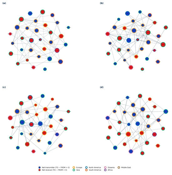
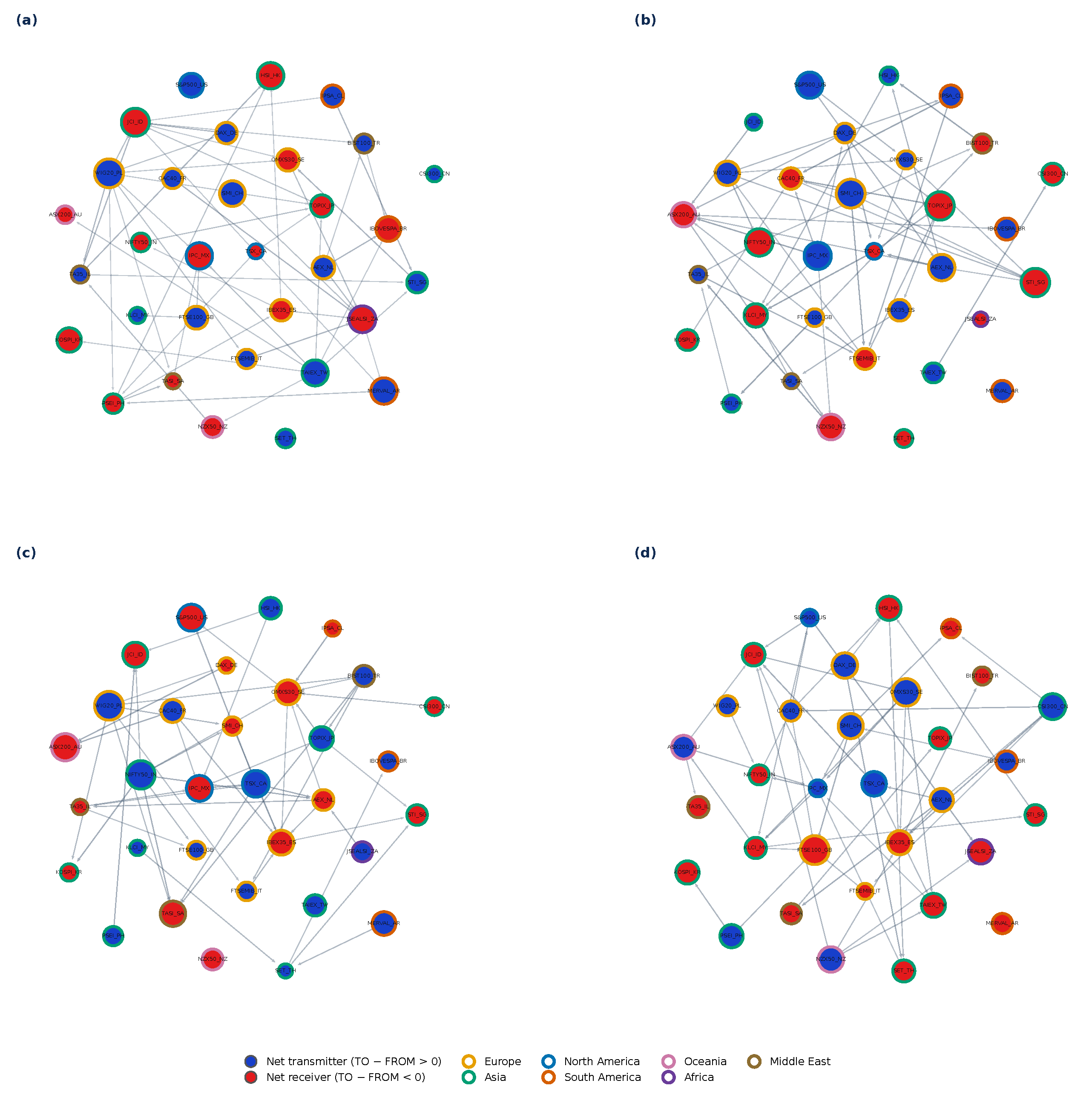
FDR diagnostics are restrictive. Under the exact circular-shift test, the smallest attainable event-level p values range from $1/149$ in the European sovereign-debt crisis to $1/201$ in the Russia–Ukraine period. No directed edge survives 5% BH-FDR in any of the four event networks. Thus, Figure 2 displays the strongest 10% of bilateral Net ETE values for descriptive comparability, not an FDR-significant backbone.

Figure 2. Event-specific bilateral Net ETE networks with a common ForceAtlas2 layout. Only the strongest 10% of bilateral Net ETE arrows are shown. Node fill denotes the sign of NET, node size is proportional to $\left|NET\right|$, and borders denote regions. Node roles use the full directed ETE matrix; GLMY topology also uses the original directed ETE matrix rather than the displayed bilateral differences. The arrows are descriptive, alignment-dependent, and not FDR-validated. (a) Global financial crisis; (b) European sovereign-debt crisis; (c) COVID-19 pandemic; (d) Russia–Ukraine war.

4.2. Temporal Dynamics of Volatility and Transmission Roles

Monthly standardized volatility exhibits pronounced temporal and regional heterogeneity across the 32 stock markets (Figure 3). A broad increase occurs during the global financial crisis, with persistent high-volatility episodes across European, Asian, and North American markets. The European sovereign-debt crisis is more regionally concentrated, although several non-European markets also show elevated values. Around the onset of COVID-19, volatility rises widely and synchronously across almost all regions, consistent with evidence of abrupt pandemic-era financial integration [15,18]. Following the Russia–Ukraine invasion, responses become more heterogeneous and are concentrated in selected European and Asian markets, in line with evidence that trade exposure and asset type condition the reaction to geopolitical shocks [16,17,19]. Thus, similar increases in volatility need not imply identical transmission architecture.

Figure 3. Temporal evolution of volatility across 32 global stock markets. Monthly volatility was standardized within each market and arranged by geographical region. Red and blue cells indicate relatively high and low volatility, respectively, with color intensity representing the magnitude of the within-market z-score. The marked periods indicate the global financial crisis, European sovereign-debt crisis, COVID-19 pandemic, and Russia–Ukraine war.

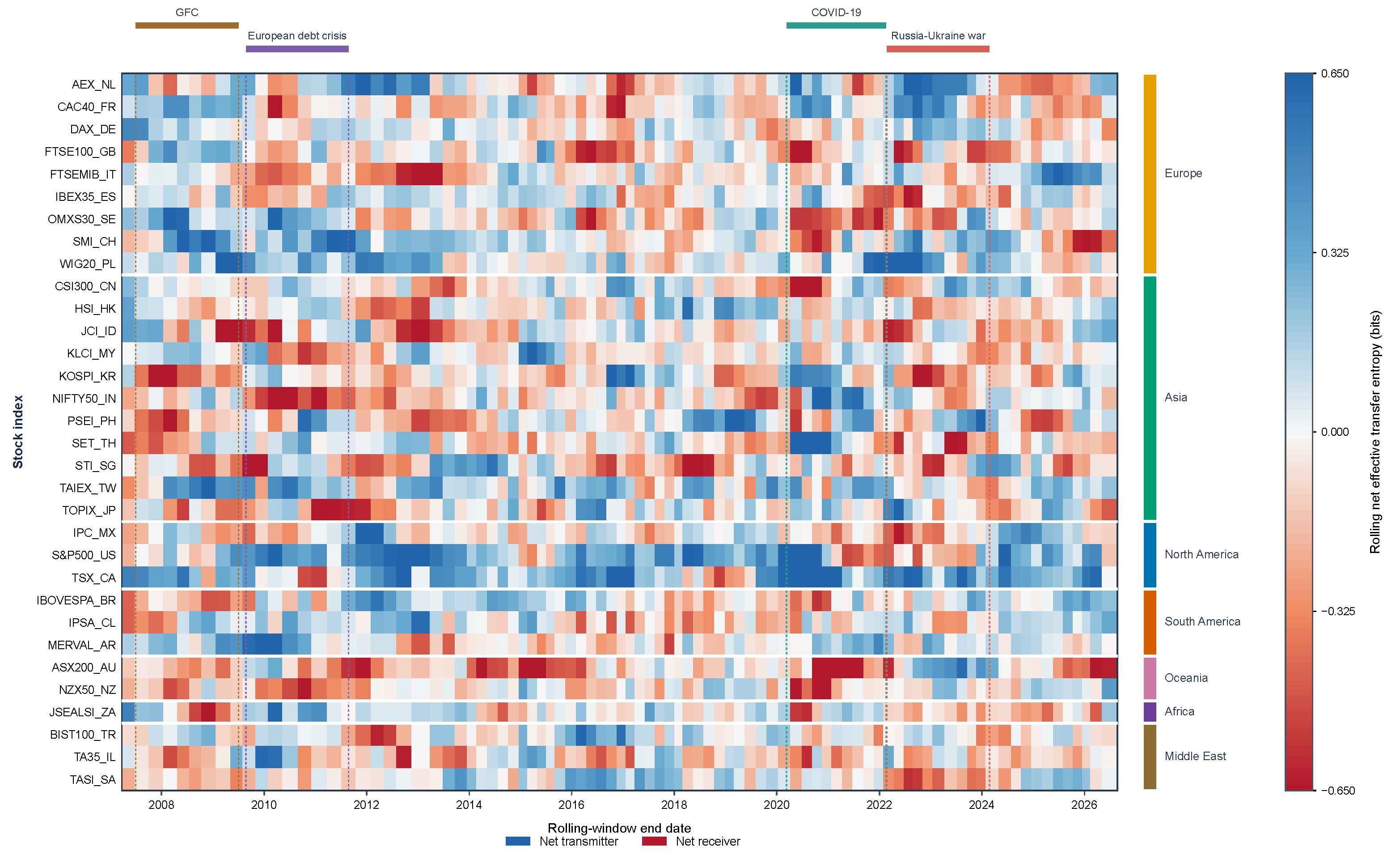
Figure 4 shows repeated changes in the sign and magnitude of rolling NET. European and North American transmitters are visible during parts of the global financial and sovereign-debt episodes, while the COVID-19 period contains a more geographically mixed set of sender and receiver phases. Roles again change after the Russia–Ukraine outbreak. These patterns are broadly consistent with crisis-dependent international connectedness [13,14,15,16,17], but small values near zero represent uncertain role differences and should not be interpreted as discrete state changes. The heat map is a descriptive summary of the bias-corrected network; it is not filtered by FDR.

Figure 4. Rolling net volatility-information transmission roles across 32 global stock markets using 120 common dates, a 20-date step, three fixed states, and all 119 distinct nonzero circular shifts. Blue and red indicate positive and negative NET, respectively; values near zero should not be read as statistically established role reversals. The color scale is truncated at the 95th percentile of $\left|NET\right|$.

4.3. Regional Information Transmission

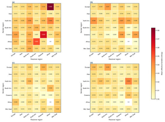
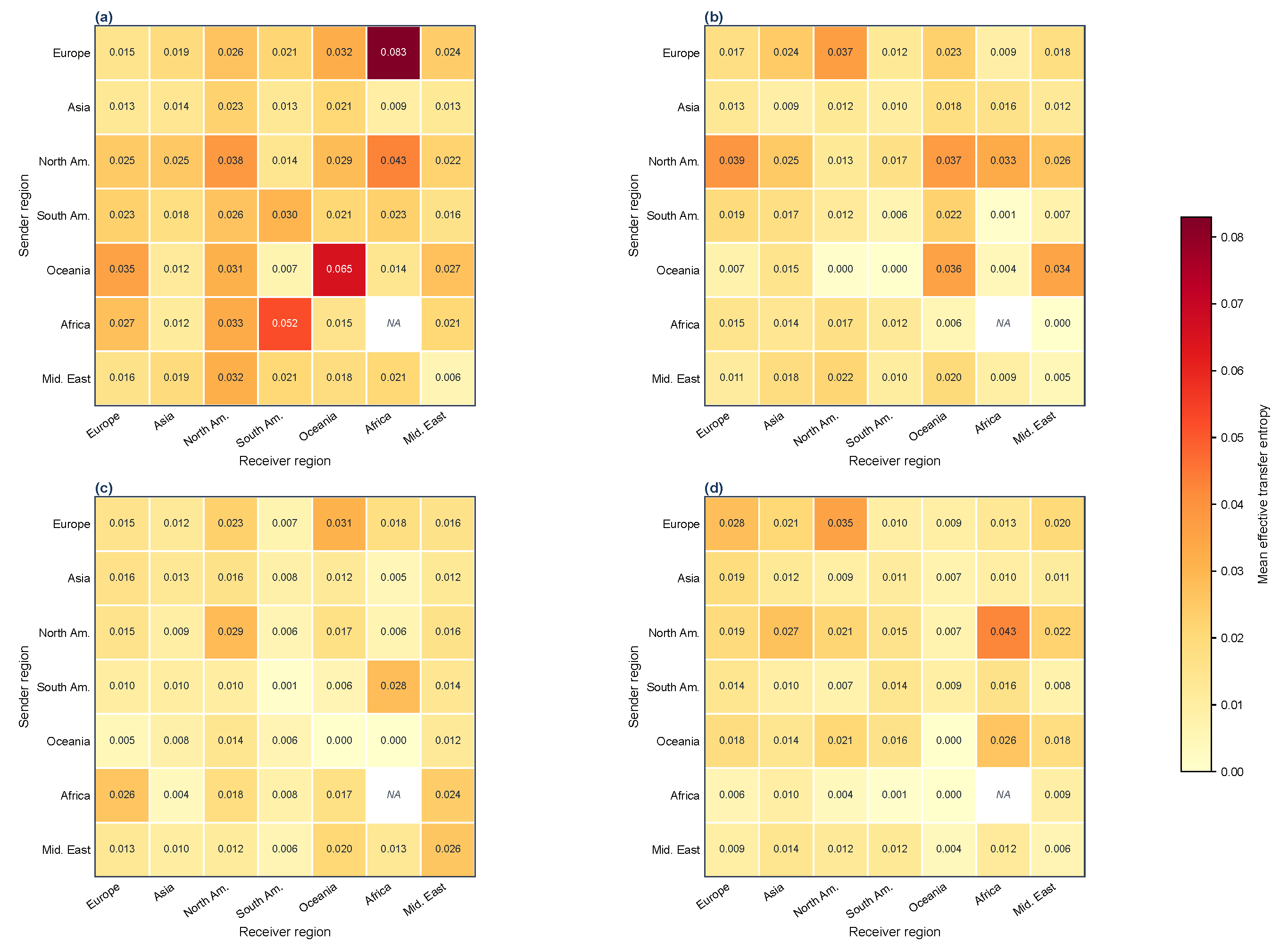
Regional means also vary by episode (Figure 5). The global financial crisis contains comparatively strong outward flows from Europe and North America, the sovereign-debt episode emphasizes transatlantic relations, COVID-19 is more dispersed, and the Russia–Ukraine period again contains a pronounced European component. Regional clustering is compatible with trade, financial integration, and common-information channels documented in contagion research [8,9], but the statements here describe the baseline matrix and are intentionally weaker than claims of geographic contagion because the uniform lag does not correct for exchange closing times [10].

Figure 5. Regional mean ETE across four events: (a) global financial crisis; (b) European sovereign-debt crisis; (c) COVID-19 pandemic; (d) Russia–Ukraine war. Rows are sender regions and columns are receiver regions. Region sizes are Europe 9, Asia 11, North America 3, South America 3, Oceania 2, Africa 1, and Middle East 3. Cross-region denominators are $|R_a\left|\right|R_b|$ and within-region denominators are $|R_a\left|\right(|R_a|-1)$. Africa-to-Africa is undefined and shown as NA.

Region sizes differ sharply, so cell precision is unequal. Europe and Asia contain 9 and 11 markets, whereas Africa contains only South Africa. Africa-to-Africa is consequently marked NA: there is no admissible within-region dyad, not an observed zero. Cells involving small regions should be treated as descriptive summaries rather than equally precise region-level estimates.

4.4. Multiscale Filtered GLMY Topology Across Crises

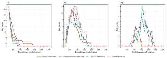
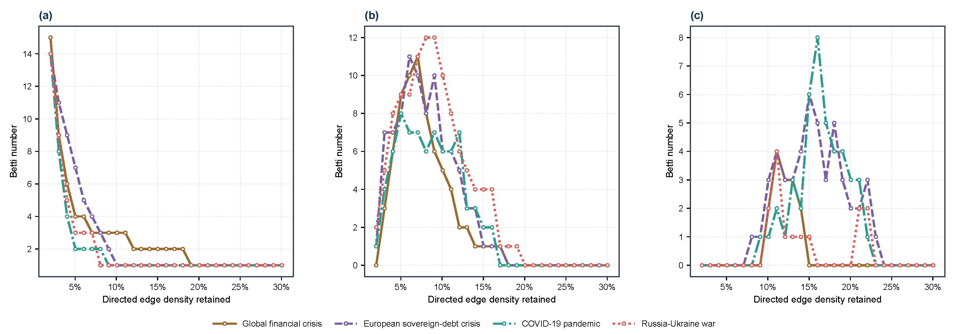
The filtered Betti curves differ across events (Figure 6 and Table 6). The strong-edge graph first reaches global weak connectivity at approximately 19% density in the global financial crisis, compared with 10% in the sovereign-debt crisis, 9% during COVID-19, and 8% during the Russia–Ukraine period. Event-sensitive topological reorganization is consistent with persistent-homology evidence that crises and major public events alter the geometry of financial dependence [48,50,52]; our result adds direction by building the filtration from ETE edges. These values concern weak connectivity: at 10% density, the corresponding LSCC shares are 0.813, 0.906, 0.625, and 0.750, so weak coverage and mutual directed reachability are not equivalent.

Figure 6. Multiscale filtered GLMY Betti curves for four event-specific directed ETE networks. (a) ${\beta }_0$, the number of weakly connected components; (b) ${\beta }_1$, the dimension of non-boundary one-dimensional path classes; (c) ${\beta }_2$, the dimension of two-dimensional path-homology classes induced by allowed directed paths. These are Betti curves over density levels, not persistence barcodes.

Table 6. Event-level intensity, concentration, integration, and filtered path-homology summaries.

Event	TETE	Edge HHI	${\mathit{\rho }}_{\mathit{c}}$	LSCC	${\mathit{A}}_1$	${\mathit{A}}_2$	FDR Edges
GFC	19.347	0.00251	0.191	0.813	0.704	0.138	0
Debt crisis	16.514	0.00305	0.101	0.906	0.878	0.491	0
COVID-19	13.094	0.00311	0.091	0.625	0.746	0.442	0
Russia–Ukraine	15.881	0.00258	0.081	0.750	1.113	0.140	0

Russia–Ukraine has the largest observed first-dimensional summary (${\beta }_1^{\max }=12$, $A_1=1.113$). The COVID-19 network reaches the largest peak ${\beta }_2$ of 8, while the sovereign-debt event has the largest integrated second-dimensional value ($A_2=0.491$). These are dimensions of path-homology groups over the baseline filtration, not counts of economic feedback loops or multi-market interactions.

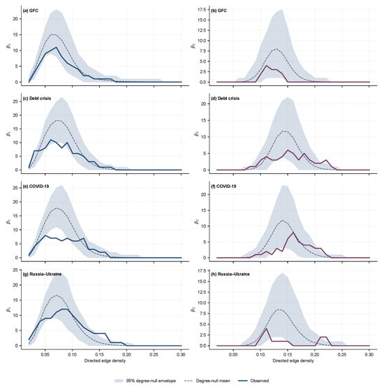
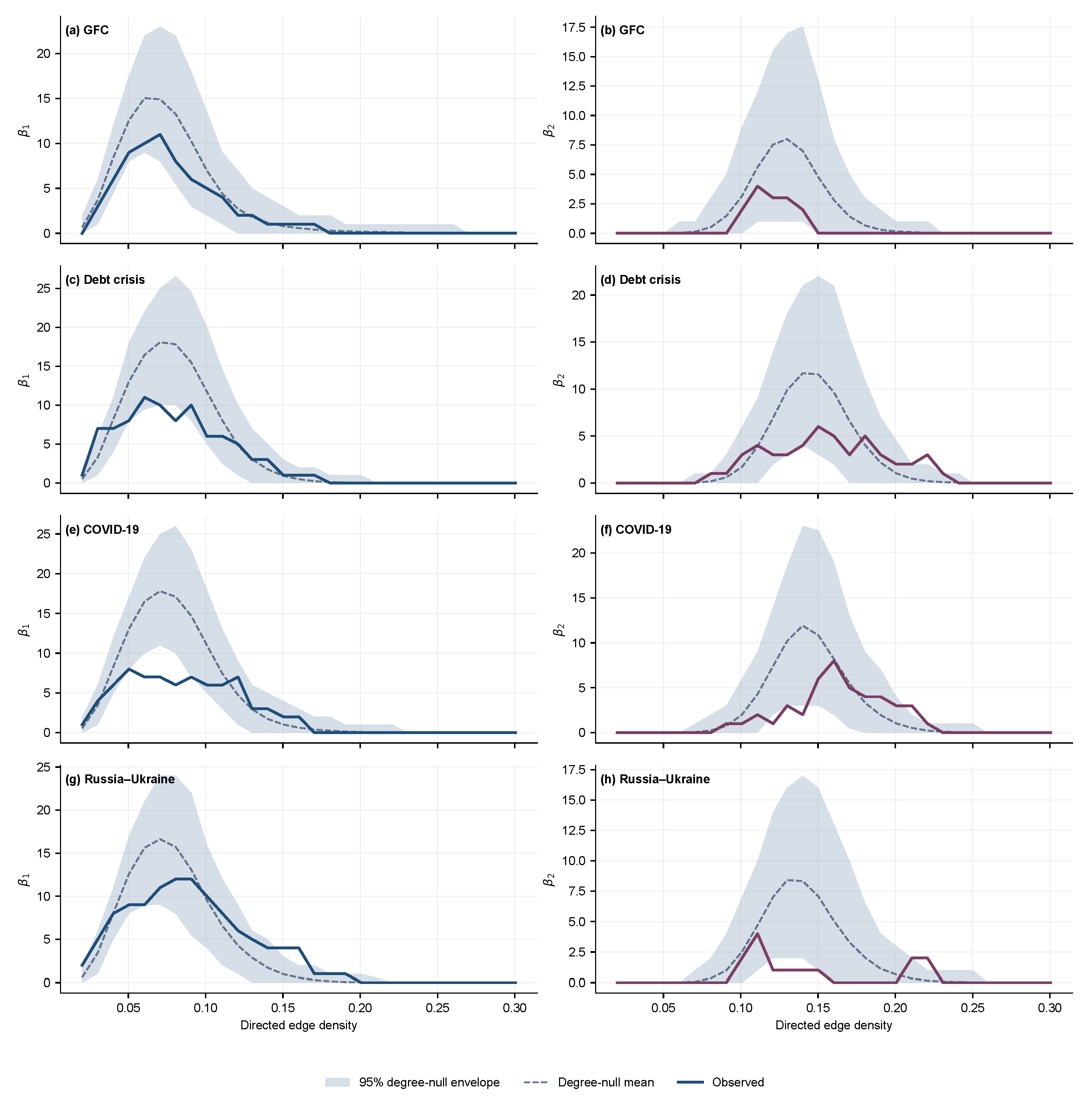
The 499-repetition maximum-density degree-conditioned edge-swap null substantially narrows the event-level claims (Figure 7). None of the four observed weak-connectivity thresholds differs from its degree-conditioned null at the nominal 5% level (two-sided Monte Carlo $p=0.148$, 0.112, 0.772, and 0.576 for the global financial, sovereign-debt, COVID-19, and Russia–Ukraine events). Three integrated summaries have nominal raw $p<0.05$: global-financial-crisis $A_2$ ($p=0.044$), COVID-19 $A_1$ ($p=0.016$), and Russia–Ukraine $A_2$ ($p=0.024$). None survives BH adjustment across the 12 event-by-summary comparisons (respectively $q=0.176$, 0.144, and 0.144). Thus, the maximum-density degree-conditioned benchmark does not provide multiplicity-adjusted evidence that an event summary departs from its null. Repeating the 499-replicate benchmark with 20 and 50 accepted swaps per edge leaves the original-support retention on a stable plateau (pooled means 0.415–0.417) and leaves all 12 comparisons above the separately adjusted 5% BH threshold at every multiplier (Supplementary Table S9). The contrast with the unrestricted null shows that the event-level conclusion is sensitive to conditioning on maximum-density degree sequences; it does not identify degree heterogeneity as a causal explanation. The 999-repetition unrestricted results are retained in Supplementary Table S9 as a sensitivity comparison.

Figure 7. Observed event-level ${\beta }_1$ and ${\beta }_2$ curves against 95% envelopes from 499 maximum-density degree-conditioned edge-swap networks. Panels (a,b), (c,d), (e,f), and (g,h) correspond respectively to the global financial crisis, European sovereign-debt crisis, COVID-19 pandemic, and Russia–Ukraine war; the left and right columns show ${\beta }_1$ and ${\beta }_2$. The null preserves each node’s in- and out-degree at the maximum analyzed density but not the strengths or the intermediate-density degree sequence.

The node-offset-consistent relative-shift network surrogate provides an aggregate temporal-alignment diagnostic (Supplementary Table S10). Event TETE exceeds its specified surrogate distribution in all four episodes (two-sided $p=0.004$, the 499-surrogate resolution limit, and BH $q=0.011$ in each case). Five of the 12 topology summaries also survive BH adjustment within the full 16-comparison event family: global-financial-crisis ${\rho }_c$ ($q=0.018$) and $A_2$ ($q=0.011$), sovereign-debt $A_1$ ($q=0.043$), COVID-19 $A_1$ ($q=0.040$), and Russia–Ukraine $A_2$ ($q=0.011$). In all four integrated-summary comparisons that remain significant after BH adjustment, the observed value lies below its surrogate distribution; the significant global-financial-crisis ${\rho }_c$ lies above its surrogate distribution. These are diagnostics of complete-network summaries within the specified relative-shift family; they neither constitute literal shifted-panel randomization inference nor identify significant bilateral channels or condition on the observed degree sequence.

No coefficient-field sensitivity was observed for the graphs analyzed here. Across all 116 event-density points and 1320 rolling-window-density points, the ${\beta }_1$ and ${\beta }_2$ values over ${\mathbb{F}}_3$ and ${\mathbb{F}}_5$ are pointwise identical to their ${\mathbb{F}}_2$ counterparts; hence all event $A_1,A_2$ summaries and the rolling associations are unchanged (Supplementary Table S8). This empirical equality is specific to the present directed graphs and is not assumed to be a general property of path homology.

At the same 10% density, binary reciprocity is 0.26, 0.12, 0.10, and 0.04 across the four events; Fagiolo transitivity is 0.177, 0.139, 0.193, and 0.113; and regional assortativity is $-0.036$, $-0.113$, 0.016, and $-0.035$. These conventional diagnostics do not reproduce a single ordering of $A_1$ or $A_2$. The comparison shows non-redundancy at the descriptive level, although it is not an incremental-prediction test.

4.5. Rolling GLMY Topology and Information-Flow Intensity

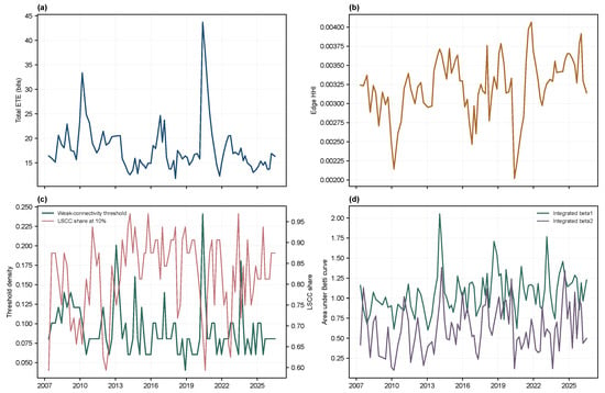
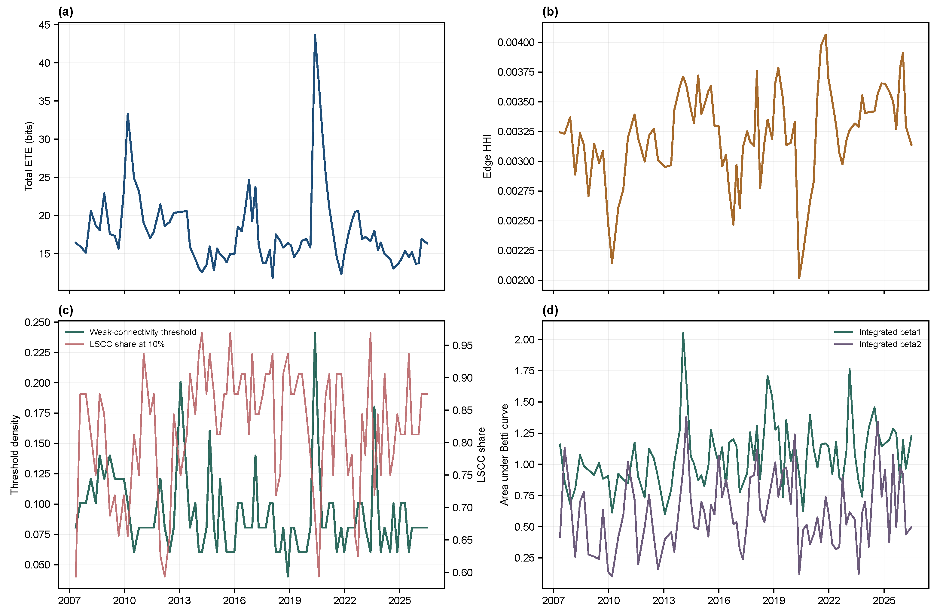
Rolling TETE reaches 43.71 bits in the window ending 20 May 2020 (Figure 8a). In that window the weak-connectivity threshold is 0.241, but the edge HHI is only 0.00202, equivalent to approximately 495 effective weighted edges. At 5% and 10% density, the strongest edges are incident to only 26 and 29 of the 32 markets, respectively; complete incident-node coverage first occurs at realized density 0.236 (Supplementary Table S4). The combination of high TETE, low HHI, and incomplete strong-edge coverage directly shows that global weight dispersion and node coverage are different properties.

Figure 8. Rolling intensity, concentration, integration, and path topology. (a) TETE; (b) edge HHI; (c) weak-connectivity threshold and LSCC share at 10% density; (d) integrated ${\beta }_1$ and ${\beta }_2$. Windows contain 120 common dates and advance by 20 dates.

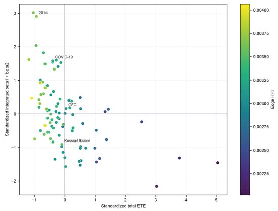
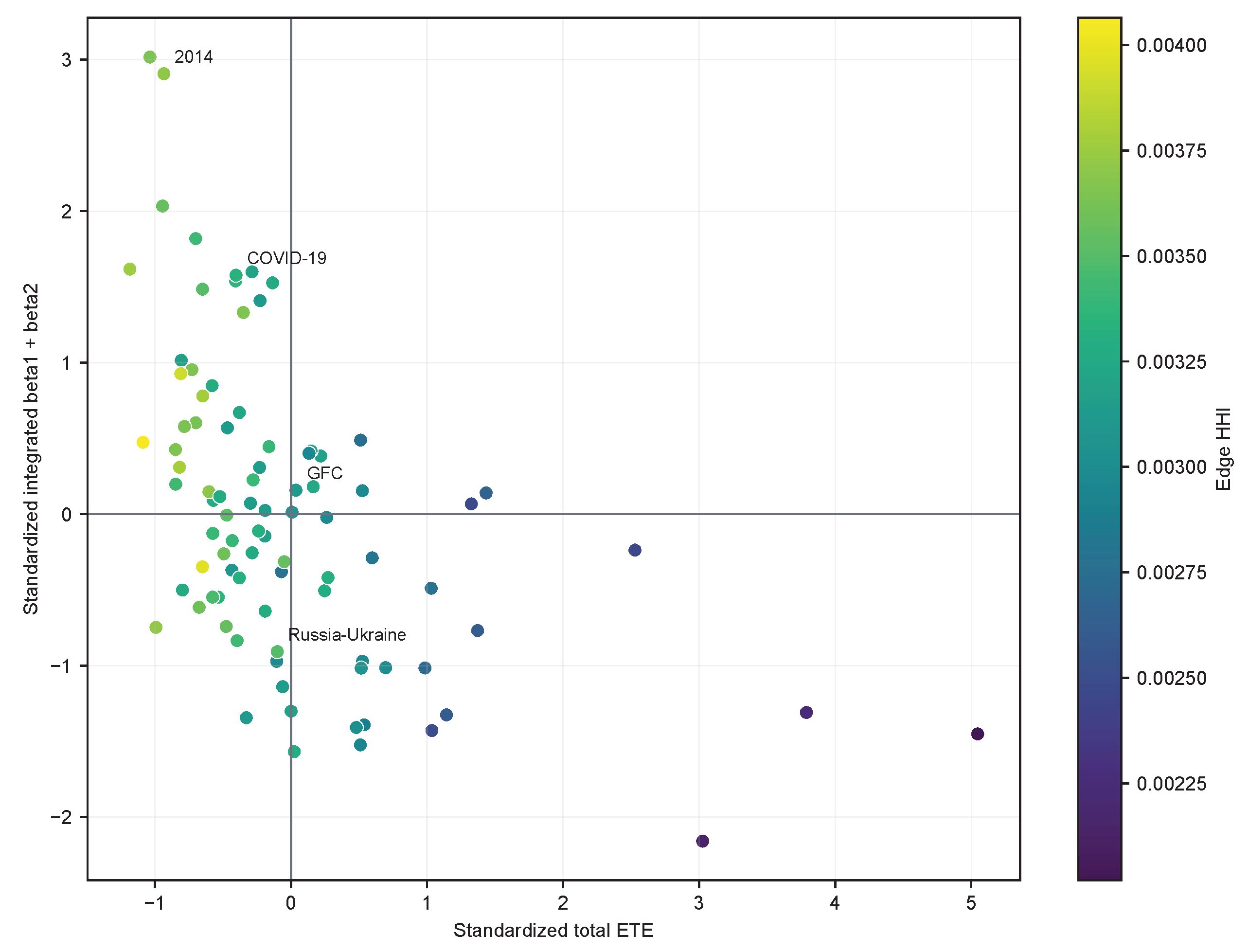
Integrated path-homology dimensions vary independently of the TETE peaks (Figure 8d). For example, the window ending 22 January 2014 has peak ${\beta }_1=31$ at TETE 13.10, and the window ending 25 March 2014 has peak ${\beta }_2=28$ at TETE 12.58. The phase diagram in Figure 9 shows observations in all four intensity–topology quadrants rather than a one-dimensional crisis ordering.

Figure 9. Intensity–topology phase diagram. The horizontal axis is standardized TETE, the vertical axis is the standardized sum $A_1+A_2$, and color denotes edge HHI. The four quadrants illustrate heterogeneous combinations of aggregate intensity and filtered path-homology organization across rolling windows. Labels mark representative windows rather than estimated change points.

Across-window moving-block resampling supports the baseline intensity–topology association (Table 7). TETE is positively associated with ${\rho }_c$ and negatively associated with $A_1$ and $A_2$. Removing the maximum-TETE window or the complete COVID-19 interval preserves these directions. Longer windows and four-state discretization also preserve the signs: $r_s(TETE,{\rho }_c)$ ranges from 0.351 to 0.566, $r_s(TETE,A_1)$ from $-0.242$ to $-0.405$, and $r_s(TETE,A_2)$ from $-0.327$ to $-0.531$. This time variation agrees with the broader evidence that TE and network connectedness change across crises and economic regimes [42,44,45], while the opposite movements of intensity and Betti summaries are specific to the present density-conditioned filtration. Full alternative-specification results are reported in Supplementary Table S2.

Table 7. Rolling Spearman associations with TETE under dependence-aware and reduced-overlap analyses.

Diagnostic	Baseline MBB	Non-Overlap	Partial Controls
Weak-connectivity threshold	0.351 [0.145, 0.505]	$-0.072$ [$-0.630$, 0.494]	$-0.002$ [$-0.197$, 0.234]
Integrated ${\beta }_1$	$-0.405$ [$-0.586$, $-0.195$]	0.189 [$-0.434$, 0.708]	$-0.122$ [$-0.321$, 0.047]
Integrated ${\beta }_2$	$-0.531$ [$-0.648$, $-0.374$]	$-0.432$ [$-0.825$, 0.163]	$-0.289$ [$-0.509$, $-0.058$]
Edge HHI	$-0.852$ [$-0.920$, $-0.748$]	$-0.818$ [$-0.967$, $-0.450$]	–

The endpoint-available within-window quantile specification likewise preserves the three signs: $r_s(TETE,{\rho }_c)=0.361$, $r_s(TETE,A_1)=-0.495$, and $r_s(TETE,A_2)=-0.486$, with moving-block intervals [0.066, 0.567], [$-0.632$, $-0.309$], and [$-0.628$, $-0.258$], respectively. Thus, the baseline pattern is not created solely by using post-window observations to set the full-sample cut points, although the within-window states are less directly comparable across dates.

The rolling weight-location benchmark places all three observed association coefficients outside their uniform edge-ordering null distributions (Supplementary Figure S1 and Table S6). Across 999 null trajectories, the 95% intervals for the three correlations are [$-0.196$, 0.207] for ${\rho }_c$, [$-0.213$, 0.207] for $A_1$, and [$-0.202$, 0.204] for $A_2$. The observed coefficients, 0.351, $-0.405$, and $-0.531$, lie outside these ranges, with conditional two-sided Monte Carlo tail areas of 0.002, 0.001, and 0.001, respectively; the latter two values are at the simulation resolution limit. This conditional diagnostic indicates that the three associations are not reproduced by independent uniform dyad orderings given the window-specific weight multisets. It is not dependence-aware inference for overlapping time series and does not validate individual ETE edges; dependence-aware uncertainty is instead supplied by the moving-block intervals and reduced-overlap analysis.

The node-offset-consistent relative-shift benchmark gives a complementary temporal-alignment diagnostic (Supplementary Table S10). Window-wise upper-tail diagnostics flag most rolling endpoints: with 499 surrogate matrices per window, observed TETE lies above the central 95% envelope in 77 of 88 windows, and 79 endpoint-wise upper-tail comparisons have BH $q<0.05$. The 100-of-120 overlap makes these flags strongly dependent, so they describe persistence under the specified surrogate family and their count is not interpreted as the number of independent discoveries. In the computationally coarser 99-surrogate topology diagnostic, observed ${\rho }_c$ lies below and above its pointwise central envelope in 1 and 7 windows, respectively; the corresponding counts are 22 and 1 for $A_1$, and 33 and 0 for $A_2$. The predominance of lower $A_p$ values is consistent with the event comparison, but these counts are envelope diagnostics under a specified relative-shift family, not fine-resolution inference or edge validation.

The uncertainty qualifications are substantive. The non-overlapping sample contains only 15 windows; its intervals include zero for ${\rho }_c$, integrated ${\beta }_1$, and integrated ${\beta }_2$. After controlling edge HHI and mean variance, the $TETE$–${\rho }_c$ partial correlation is $-0.002$ with an interval spanning zero; the integrated $H_1$ relation is also attenuated and crosses zero, whereas the integrated $H_2$ relation remains negative but smaller. Exact circular-shift testing yields zero 5% FDR edges in all 88 rolling windows. Given the coarse attainable shift p values and 992 simultaneous dyadic comparisons, the empty BH backbones indicate that individual channels cannot be validated at this sample length; they are not affirmative evidence that every dyadic effect is zero. These results support a recurring descriptive pattern, not an independent-window causal law.

Rank stability is partial and varies by diagnostic (Supplementary Table S5). The five prespecified windows end on 24 June 2009, 10 August 2011, 20 May 2020, 10 March 2022, and 31 May 2023. Under the baseline six-observation blocks, the median all-dyad rank correlation between the observed and 199 moving-block re-estimates ranges from 0.378 to 0.530, whereas median top-5% Jaccard overlap is only 0.124–0.205 and median top-10% overlap is 0.183–0.258. Block lengths three, six, and twelve preserve this qualitative contrast between the full ranking and the strongest-edge sets. The observed ${\rho }_c$, $A_1$, and $A_2$ values fall within their 95% resampling intervals in 42 of 45 block-length-by-window-by-summary comparisons; the exceptions are COVID-19 ${\rho }_c$ with three-observation blocks and global-financial-crisis $A_1$ with six- and twelve-observation blocks. These are compatibility checks with broad intervals, not evidence of precise topology estimation. Adjacent rolling windows have median all-dyad rank correlation 0.613, but the median falls to 0.021 at six-window separation. The latter comparisons measure temporal persistence, not sampling stability, and the adjacent value is inflated by the windows’ 100 shared observations. These diagnostics reinforce that monotone rank invariance is a property of the filtration and should not be read as validation of every estimated edge order.

Contrary to a simple fewer-dominant-edges mechanism, TETE is negatively correlated with edge HHI ($r_s=-0.852$, 95% interval $[-0.920,-0.748]$) and positively correlated with effective edge count ($r_s=0.852$). The sign remains negative for normalized edge HHI, which adjusts for the number of positive edges (Supplementary Tables S2 and S3). Direct coverage statistics sharpen the interpretation: $r_s(TETE,{\rho }_{\mathrm{cov}})=0.396$ (95% moving-block interval [0.194, 0.534]), while $r_s(TETE,C\left(0.05\right))=-0.359$ (interval [$-0.525$, $-0.156$]). High-intensity windows therefore use a broader effective set of weighted edges overall, even though their strongest edges cover markets less evenly. Concentration and mean-variance controls substantially attenuate the connectivity association, so the evidence supports distinct network coordinates but not a simple “fewer dominant edges” explanation.

The absolute-threshold comparison clarifies the scope of the result. Using the exact edge-weight connectivity cutoff and the common 0.06–0.15-bit grid for the Betti integrals, TETE is positively associated with the absolute connectivity cutoff ($r_s=0.575$) and with integrated absolute-threshold ${\beta }_1$ and ${\beta }_2$ ($r_s=0.784$ and 0.818; Supplementary Table S7). This reversal of the Betti-association signs is informative rather than contradictory: an absolute threshold permits high-weight windows to contain more retained edges, whereas the density filtration fixes the edge count and isolates their organization. The negative baseline TETE–Betti relation is therefore a finding about density-conditioned, rank-induced organization, not an invariant relation under every filtration.

5. Discussion and Conclusions

The central result is that information-flow intensity and density-conditioned network organization are not interchangeable. TETE measures the aggregate weight of pairwise directional predictive information, ${\rho }_c$ measures how deeply one must move down the ranked edge list to obtain global weak coverage, LSCC measures mutual directed reachability at a fixed density, and $A_1$ and $A_2$ measure dimensions of non-boundary path classes across densities. Their different temporal behavior is consistent with the complex-network view that aggregate interaction strength does not determine architecture [2,4,32]. The finding is deliberately conditional on the filtration: when one instead uses a fixed absolute ETE threshold, higher-intensity windows retain more edges and the TETE–Betti associations become positive.

The concentration and coverage analyses refine the mechanism. Higher TETE is associated with lower edge HHI and a larger effective edge count, not with a smaller set of dominant weighted edges. At the same time, the direct $C_t\left(\rho \right)$ and ${\rho }_{\mathrm{cov},t}$ statistics show that the highest-ranked subset reaches markets less evenly in high-intensity windows. A high ${\rho }_c$ can therefore coexist with low global HHI when the weight is distributed across many dyads, but some nodes enter only through weaker ranks. This distinction could not be established from TETE, concentration, centrality, or Betti curves alone.

The event results describe different architectures rather than a one-dimensional ranking of crisis severity. The sovereign-debt event has the largest observed $A_2$, and Russia–Ukraine has the largest observed $A_1$. At 10% density, LSCC shares show that weak integration and mutual reachability can diverge. Unrestricted weight-location and maximum-density degree-conditioned benchmarks are reported separately, preventing the former from being interpreted as evidence beyond degree heterogeneity. Path homology supplies a directed multiscale coordinate not identical to reciprocity, transitivity, regional assortativity, or component size; a formal incremental-prediction claim would require a separate forecasting design.

The null models answer complementary questions and should not be collapsed into a single declaration of “non-random topology.” Node-offset-consistent relative-shift surrogates indicate that aggregate event TETE is not reproduced within the specified relative-alignment family, and several event topology summaries also depart from that benchmark. Because these are not literal full-panel rotations, the evidence is diagnostic rather than exact multivariate-panel randomization inference. By contrast, no event topology summary survives multiplicity adjustment once the maximum-density in- and out-degree sequences are preserved. The combined evidence supports aggregate predictive-information structure under the retained alignment while showing that the topology conclusion is sensitive to conditioning on degree heterogeneity.

These findings extend rather than contradict the connectedness literature. Studies based on variance decompositions, TE, recurrence networks, and sectoral networks generally find stronger and time-varying interdependence during stress [24,35,36,42,45]. Correlation- and TE-based network studies in Mathematics likewise show that alternative edge definitions reveal different aspects of financial structure and portfolio risk [34,37]. Our results add that a rise in total directional information can coincide with weaker strong-edge coverage and smaller integrated directed path-homology dimensions. The contribution is therefore not another crisis-intensity index, but a decomposition of intensity, dispersion, integration, and directed higher-order organization.

The rolling signs persist across 120-, 180-, and 240-date windows, three- versus four-state discretization, the endpoint-available within-window cut-point sensitivity, and coefficients in ${\mathbb{F}}_2$, ${\mathbb{F}}_3$, and ${\mathbb{F}}_5$. Moving-block intervals and crisis-exclusion checks support the baseline pattern, but the reduced non-overlapping sample is small and imprecise. Controls for edge HHI and mean variance attenuate the associations and reduce the $TETE$–${\rho }_c$ relation to approximately zero. Null and rank-stability diagnostics further support a cautious interpretation: they assess whether the pipeline reproduces the observed summaries under specified perturbations, but they do not convert empty edgewise FDR backbones into validated transmission channels. The evidence is best described as a dependence-aware structural diagnostic, not a predictive early-warning system or a causal response of topology to information intensity.

Several limitations materially bound interpretation. First, only 27.29% of outer-calendar dates survive the strict intersection, and 120 observations can span 651 calendar days. Uniform lag-one alignment uses t to predict $t+1$, rather than a later close to predict an earlier close on the same date, but it still does not equalize elapsed clock time across regional pairs. Both sender–receiver labels and the directed edge ordering that induces the path-homology filtration remain conditional on the retained common-observation alignment. Second, pairwise ETE does not remove common global factors or indirect paths. Third, all event and rolling networks have empty 5% FDR backbones under the exact edgewise shift test, whose attainable p values are coarse in short windows; positive ETE filtrations remain descriptive. The node-offset-consistent relative-shift network surrogate couples those exact edgewise shift supports, but because the estimator uses $T-1$ linear transitions, it is not a literal re-estimation of independently rotated complete panels. Fourth, the maximum-density degree-conditioned edge-swap null conditions on degrees only at the maximum analyzed density and not on strengths or every intermediate filtration level. Fifth, selected-window block resampling and temporal rank comparisons reveal uncertainty in the estimated order and do not validate every edge rank. Finally, within-window cut points remove future observations beyond each endpoint but sacrifice globally fixed state meanings; one index represents each market, and no persistence barcodes or representative generators are computed. Time-zone-aware and pairwise calendars, global-factor residualization, strength-preserving nulls, and genuine persistent path homology remain priority extensions.

Taken together, the study combines circular-shift-corrected ETE with a directed edge-density filtration and GLMY path homology for 32 global stock markets. In the baseline fixed-density comparison, higher TETE is associated with a higher density required for global weak connectivity and with smaller integrated $H_1$ and $H_2$ dimensions, while direct coverage and HHI measures distinguish uneven strong-edge reach from broad overall weight dispersion. The connectivity association is not robust to concentration and mean-variance controls, and the Betti signs reverse under an absolute threshold, so the conclusion is specific to rank-conditioned organization. The construction is an alignment-dependent structural diagnostic, not evidence of structural causality or a validated crisis-warning rule. More generally, total interaction strength is not a substitute for network architecture.

References

- Schweitzer, F.; Fagiolo, G.; Sornette, D.; Vega-Redondo, F.; Vespignani, A.; White, D.R. Economic networks: The new challenges. Science 2009, 325, 422–425. [Google Scholar] [CrossRef] [Scilit] [PubMed]
- Haldane, A.G.; May, R.M. Systemic risk in banking ecosystems. Nature 2011, 469, 351–355. [Google Scholar] [CrossRef] [Scilit] [PubMed]
- Acemoglu, D.; Carvalho, V.M.; Ozdaglar, A.; Tahbaz-Salehi, A. The network origins of aggregate fluctuations. Econometrica 2012, 80, 1977–2016. [Google Scholar] [CrossRef] [Scilit]
- Acemoglu, D.; Ozdaglar, A.; Tahbaz-Salehi, A. Systemic risk and stability in financial networks. Am. Econ. Rev. 2015, 105, 564–608. [Google Scholar] [CrossRef] [Scilit]
- Caccioli, F.; Barucca, P.; Kobayashi, T. Network models of financial systemic risk: A review. J. Comput. Soc. Sci. 2018, 1, 81–114. [Google Scholar] [CrossRef] [Scilit]
- Longin, F.; Solnik, B. Extreme correlation of international equity markets. J. Financ. 2001, 56, 649–676. [Google Scholar] [CrossRef] [Scilit]
- Forbes, K.J.; Rigobon, R. No contagion, only interdependence: Measuring stock market comovements. J. Financ. 2002, 57, 2223–2261. [Google Scholar] [CrossRef] [Scilit]
- Bekaert, G.; Harvey, C.R.; Ng, A. Market integration and contagion. J. Bus. 2005, 78, 39–69. [Google Scholar] [CrossRef] [Scilit] [PubMed]
- Beine, M.; Cosma, A.; Vermeulen, R. The dark side of global integration: Increasing tail dependence. J. Bank. Financ. 2010, 34, 184–192. [Google Scholar] [CrossRef] [Scilit]
- Výrost, T.; Lyócsa, S.; Baumöhl, E. Granger causality stock market networks: Temporal proximity and preferential attachment. Physica A 2015, 427, 262–276. [Google Scholar] [CrossRef] [Scilit]
- King, M.A.; Wadhwani, S. Transmission of volatility between stock markets. Rev. Financ. Stud. 1990, 3, 5–33. [Google Scholar] [CrossRef] [Scilit]
- Hamao, Y.; Masulis, R.W.; Ng, V. Correlations in price changes and volatility across international stock markets. Rev. Financ. Stud. 1990, 3, 281–307. [Google Scholar] [CrossRef] [Scilit]
- Dungey, M.; Gajurel, D. Equity market contagion during the global financial crisis: Evidence from the world’s eight largest economies. Econ. Syst. 2014, 38, 161–177. [Google Scholar] [CrossRef] [Scilit]
- De Bruyckere, V.; Gerhardt, M.; Schepens, G.; Vander Vennet, R. Bank/sovereign risk spillovers in the European debt crisis. J. Bank. Financ. 2013, 37, 4793–4809. [Google Scholar] [CrossRef] [Scilit]
- Cheng, T.; Liu, J.; Yao, W.; Zhao, A.B. The impact of COVID-19 pandemic on the volatility connectedness network of global stock market. Pac.-Basin Financ. J. 2022, 71, 101678. [Google Scholar] [CrossRef] [Scilit]
- Tajaddini, R.; Gholipour, H.F. Trade dependence and stock market reaction to the Russia–Ukraine war. Int. Rev. Financ. 2023, 23, 680–691. [Google Scholar] [CrossRef] [Scilit]
- Umar, Z.; Polat, O.; Choi, S.-Y.; Teplova, T. The impact of the Russia–Ukraine conflict on the connectedness of financial markets. Financ. Res. Lett. 2022, 48, 102976. [Google Scholar] [CrossRef] [Scilit]
- Zhang, D.; Hu, M.; Ji, Q. Financial markets under the global pandemic of COVID-19. Financ. Res. Lett. 2020, 36, 101528. [Google Scholar] [CrossRef] [Scilit] [PubMed]
- Boungou, W.; Yatie, A. The impact of the Ukraine–Russia war on world stock market returns. Econ. Lett. 2022, 215, 110516. [Google Scholar] [CrossRef] [Scilit]
- Jareno, F.; Escribano, A.; Koczar, M.W. Non-linear interdependencies between international stock markets: The Polish and Spanish case. Mathematics 2021, 9, 6. [Google Scholar] [CrossRef] [Scilit]
- Diebold, F.X.; Yilmaz, K. Measuring financial asset return and volatility spillovers, with application to global equity markets. Econ. J. 2009, 119, 158–171. [Google Scholar] [CrossRef] [Scilit]
- Billio, M.; Getmansky, M.; Lo, A.W.; Pelizzon, L. Econometric measures of connectedness and systemic risk in the finance and insurance sectors. J. Financ. Econ. 2012, 104, 535–559. [Google Scholar] [CrossRef] [Scilit]
- Diebold, F.X.; Yilmaz, K. On the network topology of variance decompositions: Measuring the connectedness of financial firms. J. Econom. 2014, 182, 119–134. [Google Scholar] [CrossRef] [Scilit]
- Diebold, F.X.; Yilmaz, K. Better to give than to receive: Predictive directional measurement of volatility spillovers. Int. J. Forecast. 2012, 28, 57–66. [Google Scholar] [CrossRef] [Scilit]
- Adrian, T.; Brunnermeier, M.K. CoVaR. Am. Econ. Rev. 2016, 106, 1705–1741. [Google Scholar] [CrossRef] [Scilit]
- Demirer, M.; Diebold, F.X.; Liu, L.; Yilmaz, K. Estimating global bank network connectedness. J. Appl. Econom. 2018, 33, 1–15. [Google Scholar] [CrossRef] [Scilit]
- Barunik, J.; Krehlik, T. Measuring the frequency dynamics of financial connectedness and systemic risk. J. Financ. Econom. 2018, 16, 271–296. [Google Scholar] [CrossRef] [Scilit]
- Wu, J.; Yao, J.; Sun, J. Risk propagation and system resilience in sustainable–digital finance: A time–frequency higher-order moment analysis of green finance, green cryptocurrency, and non-green cryptocurrency markets. Systems 2026, 14, 628. [Google Scholar] [CrossRef] [Scilit]
- Yao, J.; Wu, J.; Feng, H.; Sun, J. Supply chain shocks and the reconfiguration of green finance markets: A quantile-on-quantile connectedness analysis. Systems 2026, 14, 652. [Google Scholar] [CrossRef] [Scilit]
- Gu, Q.; Liu, Y.; Wu, J.; Zhu, X. How stablecoins reshape interactions within a fragmented USD-access system: Evidence from a time-frequency TVP-VAR connectedness model. Systems 2026, 14, 932. [Google Scholar] [CrossRef] [Scilit]
- Battiston, S.; Puliga, M.; Kaushik, R.; Tasca, P.; Caldarelli, G. DebtRank: Too central to fail? Financial networks, the FED and systemic risk. Sci. Rep. 2012, 2, 541. [Google Scholar] [CrossRef] [Scilit] [PubMed]
- Battiston, S.; Farmer, J.D.; Flache, A.; Garlaschelli, D.; Haldane, A.G.; Heesterbeek, H.; Hommes, C.; Jaeger, C.; May, R.; Scheffer, M. Complexity theory and financial regulation. Science 2016, 351, 818–819. [Google Scholar] [CrossRef] [Scilit] [PubMed]
- Gai, P.; Kapadia, S. Contagion in financial networks. Proc. R. Soc. A 2010, 466, 2401–2423. [Google Scholar] [CrossRef] [Scilit]
- Balci, M.A.; Batrancea, L.M.; Akguller, O. Network-induced soft sets and stock market applications. Mathematics 2022, 10, 3964. [Google Scholar] [CrossRef] [Scilit]
- Wang, M.; Hua, C.; Xu, H. Dynamic linkages among carbon, energy and financial markets: Multiplex recurrence network approach. Mathematics 2022, 10, 1829. [Google Scholar] [CrossRef] [Scilit]
- Su, X.; Liu, Z. Sector volatility spillover and economic policy uncertainty: Evidence from China’s stock market. Mathematics 2021, 9, 1411. [Google Scholar] [CrossRef] [Scilit]
- Ioannidis, E.; Sarikeisoglou, I.; Angelidis, G. Portfolio construction: A network approach. Mathematics 2023, 11, 4670. [Google Scholar] [CrossRef] [Scilit]
- Schreiber, T. Measuring information transfer. Phys. Rev. Lett. 2000, 85, 461–464. [Google Scholar] [CrossRef] [Scilit] [PubMed]
- Marschinski, R.; Kantz, H. Analysing the information flow between financial time series. Eur. Phys. J. B 2002, 30, 275–281. [Google Scholar] [CrossRef] [Scilit]
- Sandoval, L., Jr. Structure of a global network of financial companies based on transfer entropy. Entropy 2014, 16, 4443–4482. [Google Scholar] [CrossRef] [Scilit]
- Bekiros, S.; Nguyen, D.K.; Sandoval Junior, L.; Uddin, G.S. Information diffusion, cluster formation and entropy-based network dynamics in equity and commodity markets. Eur. J. Oper. Res. 2017, 256, 945–961. [Google Scholar] [CrossRef] [Scilit]
- Gong, C.; Tang, P.; Wang, Y. Measuring the network connectedness of global stock markets. Physica A 2019, 535, 122351. [Google Scholar] [CrossRef] [Scilit]
- Dimpfl, T.; Peter, F.J. Using transfer entropy to measure information flows between financial markets. Stud. Nonlinear Dyn. Econom. 2013, 17, 85–102. [Google Scholar] [CrossRef] [Scilit]
- Behrendt, S.; Dimpfl, T.; Peter, F.J.; Zimmermann, D.J. RTransferEntropy—Quantifying information flow between different time series using effective transfer entropy. SoftwareX 2019, 10, 100265. [Google Scholar] [CrossRef] [Scilit]
- Almeida, D.; Dionísio, A.; Ferreira, P.; Aslam, F.; Quintino, D. Information flow between asset classes during extreme events. Physica A 2025, 671, 130687. [Google Scholar] [CrossRef] [Scilit]
- Mantegna, R.N. Hierarchical structure in financial markets. Eur. Phys. J. B 1999, 11, 193–197. [Google Scholar] [CrossRef] [Scilit]
- Tumminello, M.; Di Matteo, T.; Aste, T.; Mantegna, R.N. Correlation based networks of equity returns sampled at different time horizons. Eur. Phys. J. B 2007, 55, 209–217. [Google Scholar] [CrossRef] [Scilit]
- Gidea, M.; Katz, Y. Topological data analysis of financial time series: Landscapes of crashes. Physica A 2018, 491, 820–834. [Google Scholar] [CrossRef] [Scilit]
- Yen, P.T.-W.; Cheong, S.A. Using topological data analysis (TDA) and persistent homology to analyze the stock markets in Singapore and Taiwan. Front. Phys. 2021, 9, 572216. [Google Scholar] [CrossRef] [Scilit]
- Akingbade, S.W.; Gidea, M.; Manzi, M.; Nateghi, V. Why topological data analysis detects financial bubbles? Commun. Nonlinear Sci. Numer. Simul. 2024, 128, 107665. [Google Scholar] [CrossRef] [Scilit]
- Majumdar, S.; Laha, A.K. Clustering and classification of time series using topological data analysis with applications to finance. Expert Syst. Appl. 2020, 162, 113868. [Google Scholar] [CrossRef] [Scilit]
- Guo, H.; Ming, Z.; Xing, B. Topological data analysis of Chinese stocks’ dynamic correlations under major public events. Front. Phys. 2023, 11, 1253953. [Google Scholar] [CrossRef] [Scilit]
- Wei, Y.; Watada, J.; Wang, Z. Topology unveiled: A new horizon for economic and financial modeling. Mathematics 2025, 13, 325. [Google Scholar] [CrossRef] [Scilit]
- Grigor’yan, A.A.; Lin, Y.; Muranov, Y.V.; Yau, S.-T. Path complexes and their homologies. J. Math. Sci. 2020, 248, 564–599. [Google Scholar] [CrossRef] [Scilit]
- Chowdhury, S.; Memoli, F. Persistent path homology of directed networks. In Proceedings of the Twenty-Ninth Annual ACM-SIAM Symposium on Discrete Algorithms (SODA), New Orleans, LA, USA, 7–10 January 2018; pp. 1152–1169. [Google Scholar] [CrossRef] [Scilit]
- Chowdhury, S.; Huntsman, S.; Yutin, M. Path homologies of motifs and temporal network representations. Appl. Netw. Sci. 2022, 7, 4. [Google Scholar] [CrossRef] [Scilit]
- Garman, M.B.; Klass, M.J. On the estimation of security price volatilities from historical data. J. Bus. 1980, 53, 67–78. [Google Scholar] [CrossRef] [Scilit] [PubMed]
- Jacomy, M.; Venturini, T.; Heymann, S.; Bastian, M. ForceAtlas2, a continuous graph layout algorithm for handy network visualization designed for the Gephi software. PLoS ONE 2014, 9, e98679. [Google Scholar] [CrossRef] [Scilit] [PubMed]
Disclaimer/Publisher’s Note: The statements, opinions and data contained in all publications are solely those of the individual author(s) and contributor(s) and not of MDPI and/or the editor(s). MDPI and/or the editor(s) disclaim responsibility for any injury to people or property resulting from any ideas, methods, instructions or products referred to in the content. |
© 2026 by the authors. Licensee MDPI, Basel, Switzerland. This article is an open access article distributed under the terms and conditions of the Creative Commons Attribution (CC BY) license.