Delay-Induced Stability Switching and Optimal Control of an Information Propagation Model with Information-Holding Behavior

Abstract

People who benefit from valuable information do not always pass it on. We develop a delayed IHSCR information propagation model in which a beneficiary can either continue spreading the information or hold it after a behavioral decision lag. The key modeling distinction is that information acquisition and the subsequent sharing-or-holding decision are treated as separate behavioral stages, while information holders can also suppress active spreaders. The delayed transitions are written as outflow rates, so arbitrary nonnegative histories do not automatically preserve positivity. We therefore work with nonnegative-feasible histories and show that such histories exist near each positive equilibrium on any fixed finite interval. For zero delay, we derive the basic reproduction number, prove global asymptotic stability of the information-free equilibrium when $R_0<1$, and give Routh–Hurwitz conditions for local stability of the positive equilibrium. With the delay as a bifurcation parameter, the linearized system gives a transcendental characteristic equation and a quartic frequency equation. The critical delay is recovered from an atan2-based phase condition, and the transversality condition identifies the first spectral stability switch. For the stability-switching parameter set, an independent characteristic-root computation verifies a unique simple crossing, and a characteristic-matrix normal-form calculation gives a negative first Lyapunov coefficient, classifying the local Hopf bifurcation as supercritical with a locally orbitally stable periodic branch. We also prove the existence of a delayed optimal control on the nonnegative-feasible set and derive the optimality system, including advanced adjoint terms. At the baseline cost weights, the computed dynamic control gives a modestly higher net objective than a numerically optimized constant-control benchmark, and this ordering persists when the relative cost ratio $c_1/c_2$ is varied from 1 to 100. A two-parameter sensitivity analysis shows how the beneficiary-to-spreader and beneficiary-to-holder transition rates shift the first critical delay.

1. Introduction

Obtaining useful information does not automatically lead to continued sharing. Studies of knowledge contribution show that sharing decisions depend on motivation, social relationships, expected returns, and organizational context [1,2,3]. Work on information withholding, knowledge hiding, and knowledge hoarding also shows that people may deliberately retain information even when sharing is a recognized norm [4,5,6,7,8]. Most of this evidence comes from organizational and knowledge-management settings rather than propagation models. Still, it points to a simple distinction: benefiting from information is not the same as deciding to share it.

Consider a student preparing for an exam. The student finds a useful study method in an experience post or a study group and benefits from it. The student may then share the method with others and become a spreader. Another choice is to keep it private to preserve a competitive advantage or an information gap; this behavior corresponds to an information holder. Holders may also challenge, report, pressure, or otherwise discourage active spreaders, so some spreaders stop disseminating the information. The choice is not immediate. It takes time to understand the information, compare options, and decide what to do. This example motivates the branching from H to S or C, the holder-mediated $S\to R$ mechanism, and the decision delay $\tau$ in our model.

Compartmental and network-based models are widely used to describe transitions among information or rumor states. The classical Daley–Kendall model gave an epidemic-like description of rumor transmission [9]. Later studies considered small-world and complex networks, modular structures, heterogeneous contacts, forgetting and remembering, and other behavioral mechanisms [10,11,12,13,14,15,16,17,18]. Our previous work added an information-beneficiary state and studied its threshold, equilibrium stability, network effects, and optimal intervention [19]. That earlier model distinguished beneficiaries from other propagation states, but it stopped at information benefit: it did not represent a subsequent choice between continued sharing and information holding, nor a holder-mediated feedback on active spreaders. The present work therefore focuses on what happens after a person has benefited from the information rather than simply adding another state to the previous model.

Time delay has also been studied in rumor and information dynamics. Previous models include spatial diffusion with delay, delayed saturation control, carrier compartments, multilingual inhibition, media-reporting delays, multilayer transmission, heterogeneous networks, and multiple delays [20,21,22,23,24,25,26,27,28,29,30,31]. These studies show that delay can move characteristic roots, change equilibrium stability, and under suitable conditions produce oscillations or Hopf bifurcation. Our contribution is not simply to add a delay or repeat a Hopf analysis. A broader complex-systems perspective is provided by local-activity theory for reaction–diffusion cellular nonlinear networks, where local dynamics and spatial coupling are used to study the emergence of complex collective behavior [32]. The present IHSCR system has no diffusion operator, so that theory is not invoked in the current analysis; it instead suggests a natural framework for a future spatially coupled extension of the information-holding model.

Optimal control is also common in rumor-propagation models. Existing studies use continuous controls, media intervention, isolation, network-based measures, and delayed controls [33,34,35,36,37,38,39,40]. The question in this paper is narrower. Once a person has benefited from valuable information, that person may keep spreading it or may hold it, and this choice can take time. Few compartmental models combine this post-benefit branch with a decision delay on the branch itself. We ask two questions: can this delay destabilize a persistent propagation state, and how should controls acting on the two holding-related channels change over time?

Several recent studies are closely related to this work. Zhang et al. [19] introduced an information-beneficiary state and examined network effects and optimal control, but they did not include a delayed choice after a person had benefited from the information. Li and Ma [35] studied a delayed rumor model with optimal control. Luo et al. [28] considered delay and control on heterogeneous networks, while Yue and Huo [37] investigated an ISCR model with time delay on a scale-free network. Ding et al. [38] also studied delayed rumor dynamics on complex networks with a saturated conversion mechanism. Taken together, these studies establish that delay, network heterogeneity, and optimal intervention can be important in rumor or information dynamics, but they do not address the same post-benefit mechanism considered here. The present model combines three linked ingredients: an explicit beneficiary state, a delayed branch from that state into continued sharing or information holding, and a holder-mediated suppression channel acting back on spreaders. This mechanism-level comparison is the basis for the distinction from our earlier beneficiary model and from the closest delayed propagation models.

We develop a delayed IHSCR model that separates continued spreading from information holding after a person obtains value from the information. The modeling contribution is the post-benefit branch $H\to S$ or $H\to C$ together with the holder-mediated feedback $S\to R$, which separates acquisition of information value from the later decision to share or retain it. The dynamical contribution is to place the behavioral delay on this branch and determine how it changes the stability of the persistent propagation state; at the first critical point, the first Lyapunov coefficient further identifies the local Hopf direction and periodic-branch stability. The control contribution is a pair of interventions tied directly to the two holding-related channels; because the beneficiary state is delayed, their optimality system contains advanced adjoint terms at $t+\tau$.

The remainder of this paper is organized as follows. Section 2 presents the delayed IHSCR model and its basic properties. Section 3 analyzes equilibrium stability in the absence of behavioral delay. Section 4 investigates delay-induced stability switching and the local Hopf bifurcation at the first critical point. Section 5 formulates the delayed optimal control problem. Numerical results are presented in Section 6. Section 7 gives a two-parameter sensitivity analysis of the first critical delay, and the main conclusions are given in Section 8.

2. Model Formulation and Basic Properties

2.1. Behavioral Mechanism and Model Assumptions

We consider an open information propagation system in which individuals can enter or leave over time. The population is divided into five behavioral states: receptive individuals $I\left(t\right)$, information beneficiaries $H\left(t\right)$, information spreaders $S\left(t\right)$, information holders $C\left(t\right)$, and information-immune individuals $R\left(t\right)$. The state variables are nonnegative dimensionless densities. They are not fractions, so they do not need to sum to one.

A receptive individual becomes an information beneficiary after effective contact with a spreader. The contact term is $\alpha ⟨k⟩I\left(t\right)S\left(t\right)$, where $\alpha$ is the effective transmission rate and $⟨k⟩$ is the average network degree. Network structure is represented only by this average degree. We do not split the population by node degree or use an explicit degree distribution.

A beneficiary does not necessarily spread the information immediately after gaining value from it. The person makes a behavioral choice after a delay $\tau$. Beneficiaries then move to the spreader state at rate $\beta$ or to the information-holder state at rate $\gamma$. Here, $\beta$ and $\gamma$ are continuous-time transition rates, not two mutually exclusive probabilities, so $\beta +\gamma =1$ is not required. The delay $\tau$ is used as a population-level behavioral-response lag: the aggregate post-benefit transition rates at time t depend on the beneficiary state observed $\tau$ time units earlier. This is a phenomenological delayed-rate formulation rather than a cohort or fixed-maturation model that tracks the specific individuals who entered state H at time $t-\tau$. Accordingly, $\tau$ should not be interpreted as a fixed residence time that every beneficiary must complete before leaving state H.

Spreaders leave the active propagation process at rate $\xi$, while information holders leave the holding state at rate $\eta$. Holders may also interfere with active spreading through contact with spreaders. This interaction is represented by $\epsilon ⟨k⟩S\left(t\right)C\left(t\right)$ and moves the affected spreaders to the information-immune state. The holder remains in state C, so the term is an outflow from S and an inflow into R, not an outflow from C. All five groups leave the system at rate $\mu$, and new individuals enter state I at rate B.

For convenience, define

$$\kappa =\alpha ⟨k⟩,q=\epsilon ⟨k⟩.$$

(1)

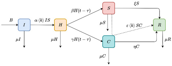
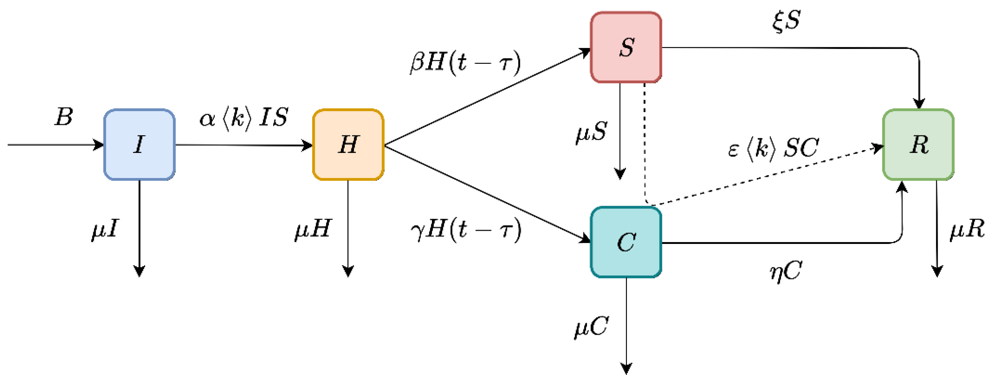
The main variables and parameters are summarized in Table 1. The state-transition structure of the model is summarized in Figure 1.

Table 1. Variables and parameters of the delayed IHSCR information propagation model.

Symbol	Description
$I\left(t\right)$	Density of receptive individuals at time t
$H\left(t\right)$	Density of information beneficiaries at time t
$S\left(t\right)$	Density of information spreaders at time t
$C\left(t\right)$	Density of information holders at time t
$R\left(t\right)$	Density of information-immune individuals at time t
B	External standardized population inflow rate
$\alpha$	Effective contact transmission rate
$\beta$	Transition rate from beneficiaries to spreaders
$\gamma$	Transition rate from beneficiaries to information holders
$\epsilon$	Effective contact-intervention rate of holders on spreaders
$\xi$	Natural forgetting rate of spreaders
$\eta$	Natural forgetting rate of information holders
$\mu$	Natural removal rate from the system
$\tau$	Behavioral decision delay
$⟨k⟩$	Average degree of the network

Figure 1. State-transition diagram of the delayed IHSCR information propagation model. The dashed $S\to R$ arrow represents the holder-dependent transfer $qSC$; the holder participates in the interaction but remains in state C.

2.2. Delayed IHSCR Information Propagation Model

According to the above transition mechanisms, the delayed IHSCR information propagation model is

$$\left\{\begin{array}{cc}\hfill \dot{I}\left(t\right)& =B-\kappa I\left(t\right)S\left(t\right)-\mu I\left(t\right),\hfill \\ \hfill \dot{H}\left(t\right)& =\kappa I\left(t\right)S\left(t\right)-\beta H(t-\tau )-\gamma H(t-\tau )-\mu H\left(t\right),\hfill \\ \hfill \dot{S}\left(t\right)& =\beta H(t-\tau )-qS\left(t\right)C\left(t\right)-(\xi +\mu )S\left(t\right),\hfill \\ \hfill \dot{C}\left(t\right)& =\gamma H(t-\tau )-(\eta +\mu )C\left(t\right),\hfill \\ \hfill \dot{R}\left(t\right)& =qS\left(t\right)C\left(t\right)+\xi S\left(t\right)+\eta C\left(t\right)-\mu R\left(t\right).\hfill \end{array}\right.$$

(2)

This formulation separates the acquisition of information value from the subsequent decision to propagate or retain the information. In particular, the delayed terms $\beta H(t-\tau )$ and $\gamma H(t-\tau )$ describe two post-benefit behavioral transitions that occur after the decision delay $\tau$. In this aggregate representation, $H(t-\tau )$ acts as a lagged state variable that modulates the current conversion intensities; it is not intended to represent the size of a single cohort whose members entered H exactly $\tau$ time units earlier. The nonlinear term $qS\left(t\right)C\left(t\right)$ represents contact-based intervention by information holders against active spreaders.

Because Equation (2) is a delay differential system, the initial state cannot be specified only at $t=0$. We prescribe continuous history functions on the full delay interval:

$$\begin{array}{cccccc}\hfill I\left(\theta \right)& ={\varphi }_1\left(\theta \right),\hfill & \hfill H\left(\theta \right)& ={\varphi }_2\left(\theta \right),\hfill & \hfill S\left(\theta \right)& ={\varphi }_3\left(\theta \right),\hfill \\ \hfill C\left(\theta \right)& ={\varphi }_4\left(\theta \right),\hfill & \hfill R\left(\theta \right)& ={\varphi }_5\left(\theta \right),\hfill & \hfill \theta & \in [-\tau ,0],\hfill \end{array}$$

(3)

where ${\varphi }_i\left(\theta \right)\ge 0$ for $i=1,\dots ,5$. Standard retarded functional differential-equation theory gives local existence and uniqueness because the right-hand side is locally Lipschitz in the current and delayed states [41]. The interpretation as population densities additionally requires a nonnegative solution.

Remark 1. 

The phenomenological delayed-rate formulation above does not define a cohort balance law. The delayed outflow terms $-(\beta +\gamma )H(t-\tau )$ imply that an arbitrary nonnegative history is not, by itself, sufficient to make the entire nonnegative cone positively invariant: if $H\left(t\right)=0$ while $H(t-\tau )>0$, the boundary derivative can be negative. We therefore separate mathematical well-posedness from physical feasibility. Standard retarded functional differential-equation theory gives a unique local solution in the phase space $C([-\tau ,0],{\mathbb{R}}^5)$, whereas the interpretation as population densities is restricted to trajectories that remain nonnegative. For a fixed horizon $T>0$, we call a nonnegative history T-compatible if its unique solution satisfies $x\left(t\right)\in {\mathbb{R}}_{+}^5$ for all $t\in [0,T]$. Thus, T-compatibility specifies the physical domain on which the delayed-rate model is interpreted; it is not used as a substitute for positive invariance of the full cone. Lemma 1 shows that the class of compatible histories is nonempty in a neighborhood of every positive equilibrium on any finite horizon. Every delayed numerical experiment reports the minimum state value and applies no artificial state truncation. The zero-delay system is different: its nonnegative orthant is positively invariant, as shown in Lemma 2. If the intended mechanism were instead a fixed residence or maturation time, a cohort-based formulation in which the delayed flux is tied to the earlier entry flux and an appropriate survival factor would be more natural and would preserve positivity. Such a reformulation changes the governing equations and therefore requires a new threshold, stability, and control analysis; we regard it as a distinct extension rather than as the model analyzed here.

2.3. Basic Properties, Reproduction Number, and Equilibria

Let

$$N\left(t\right)=I\left(t\right)+H\left(t\right)+S\left(t\right)+C\left(t\right)+R\left(t\right).$$

(4)

Adding the five equations in Equation (2) gives

$$\dot{N}\left(t\right)=B-\mu N\left(t\right),$$

(5)

and hence

$$N\left(t\right)=\left[N\left(0\right)-{\displaystyle \frac{B}{\mu }}\right]e^{-\mu t}+{\displaystyle \frac{B}{\mu }}.$$

(6)

Therefore, ${\lim }_{t\to \infty }N\left(t\right)=B/\mu$. For the nonnegative feasible solutions considered here, all state variables are bounded by $N\left(t\right)$.

The information-free equilibrium is

$$E_0=\left({\displaystyle \frac{B}{\mu }},0,0,0,0\right).$$

(7)

For later use, define

$$a=\beta +\gamma +\mu ,b=\xi +\mu ,c=\eta +\mu .$$

(8)

Using the next-generation matrix approach with active-state vector $x={(H,S,C)}^{\mathrm{T}}$ [42] gives

$$F=\left(\begin{array}{ccc}0& \kappa I^0& 0\\ 0& 0& 0\\ 0& 0& 0\end{array}\right),V=\left(\begin{array}{ccc}a& 0& 0\\ -\beta & b& 0\\ -\gamma & 0& c\end{array}\right),I^0={\displaystyle \frac{B}{\mu }}.$$

(9)

The basic reproduction number is

$$R_0=\rho \left(F{V}^{-1}\right)={\displaystyle \frac{\alpha ⟨k⟩B\beta }{\mu (\beta +\gamma +\mu )(\xi +\mu )}}.$$

(10)

Neither $\eta$ nor $\epsilon$ appears explicitly in $R_0$. At $E_0$, $C=0$, so the nonlinear intervention term $qSC$ vanishes in the linearized system. Thus, the holder-removal parameter and holder–spreader contact coefficient do not enter the local next-generation threshold, although they can affect dynamics away from the information-free state.

Equation (10) is obtained from the zero-delay next-generation matrix. For the delayed linearization at $E_0$, substituting $\lambda =0$ also gives the factor $ab(1-R_0)$ because $e^{-\lambda \tau }=1$ at $\lambda =0$. Thus, the same value marks a possible zero-root threshold for the present delayed-rate formulation. This observation does not establish stability of $E_0$ for arbitrary positive delays; the global threshold result below is deliberately restricted to $\tau =0$.

At equilibrium, $H(t-\tau )=H^{*}$, so the equilibrium coordinates themselves do not depend explicitly on the delay. The equilibrium equations are

$$\left\{\begin{array}{cc}\hfill B-\kappa I^{*}{S}^{*}-\mu I^{*}& =0,\hfill \\ \hfill \kappa I^{*}{S}^{*}-a{H}^{*}& =0,\hfill \\ \hfill \beta H^{*}-q{S}^{*}{C}^{*}-b{S}^{*}& =0,\hfill \\ \hfill \gamma H^{*}-c{C}^{*}& =0,\hfill \\ \hfill q{S}^{*}{C}^{*}+\xi S^{*}+\eta C^{*}-\mu R^{*}& =0.\hfill \end{array}\right.$$

(11)

When $R_0>1$, Equation (2) admits a positive information propagation equilibrium. Its five components are collected in one system:

$$E^{*}=(I^{*},H^{*},S^{*},C^{*},R^{*}),\left\{\begin{array}{cccc}\hfill I^{*}& ={\displaystyle \frac{abc+q\gamma B}{\beta \kappa c+q\gamma \mu }},\hfill & \hfill H^{*}& ={\displaystyle \frac{B-\mu I^{*}}{a}},\hfill \\ \hfill S^{*}& ={\displaystyle \frac{B-\mu I^{*}}{\kappa I^{*}}},\hfill & \hfill C^{*}& ={\displaystyle \frac{\gamma H^{*}}{c}},\hfill \\ \hfill R^{*}& ={\displaystyle \frac{q{S}^{*}{C}^{*}+\xi S^{*}+\eta C^{*}}{\mu }}.\hfill & & \end{array}\right.$$

(12)

Moreover,

$${\displaystyle \frac{B}{\mu }}-I^{*}={\displaystyle \frac{c(B\beta \kappa -ab\mu )}{\mu (\beta \kappa c+q\gamma \mu )}},$$

(13)

so the positive equilibrium exists precisely when $R_0>1$.

Lemma 1. 

Let $E^{*}\in {(0,\infty )}^5$ be a positive equilibrium of Equation (2), and let $T>0$ be fixed. Then, there exists ${\delta }_T>0$ such that every continuous history $\varphi \in C([-\tau ,0],{\mathbb{R}}^5)$ satisfying

$$\parallel \varphi -E^{*}{\parallel }_{\infty }<{\delta }_T$$

(14)

generates a unique solution whose five components remain strictly positive on $[0,T]$. If $E^{*}$ is Lyapunov stable in the delay phase space, the neighborhood can be chosen so that positivity holds for all $t\ge 0$.

Proof. 

Set $m=\min \{I^{*},H^{*},S^{*},C^{*},R^{*}\}>0$ and choose $ϵ=m/2$. The constant history ${\varphi }^{*}\left(\theta \right)\equiv E^{*}$ generates the equilibrium solution $x^{*}\left(t\right)\equiv E^{*}$. By continuous dependence of retarded functional differential equations on the initial history, for every fixed $T>0$, there exists ${\delta }_T>0$ such that condition (14) implies

$$\underset{0\le t\le T}{\sup }{\parallel x(t;\varphi )-E^{*}\parallel }_{\infty }<{\displaystyle \frac{m}{2}}.$$

(15)

After reducing ${\delta }_T$ if necessary, we may also take ${\delta }_T<m/2$, so the history itself is strictly positive on $[-\tau ,0]$. Hence, each component satisfies $x_i\left(t\right)>m/2>0$ on $[0,T]$. If $E^{*}$ is Lyapunov stable, the same $ϵ$-neighborhood can be maintained for all future time by choosing the initial history sufficiently close to $E^{*}$, which gives the second statement.    □

In particular, Lemma 1 provides an explicit nonempty class of histories whose uncontrolled trajectories are feasible on any prescribed finite horizon. This fact will be used below to verify nonemptiness of the feasible control set.

3. Stability Analysis in the Absence of Behavioral Delay

To establish a reference state for the subsequent delay analysis, we first consider the system without behavioral decision delay, i.e., $\tau =0$. Since the equation for $R\left(t\right)$ does not feed back into the equations for $I\left(t\right)$, $H\left(t\right)$, $S\left(t\right)$, and $C\left(t\right)$, the essential stability properties are determined by the first four states, while the R-direction contributes an additional negative eigenvalue $-\mu$.

Lemma 2. 

For $\tau =0$, the nonnegative orthant ${\mathbb{R}}_{+}^5$ is positively invariant. Every solution with nonnegative initial data is bounded and satisfies

$$0\le N\left(t\right)\le \max \left\{N\left(0\right),{\displaystyle \frac{B}{\mu }}\right\},t\ge 0.$$

(16)

Proof. 

On the coordinate boundaries $I=0$, $H=0$, $S=0$, $C=0$, and $R=0$, the corresponding derivatives of the zero-delay system are B, $\kappa IS$, $\beta H$, $\gamma H$, and $qSC+\xi S+\eta C$, respectively. They are all nonnegative whenever the remaining coordinates are nonnegative. Hence, ${\mathbb{R}}_{+}^5$ is positively invariant. Equation (6) then gives bound (16).    □

3.1. Local Stability of the Information-Free Equilibrium

At $E_0$, the characteristic equation is

$${(\lambda +\mu )}^2(\lambda +c)\left[(\lambda +a)(\lambda +b)-\beta \kappa I^0\right]=0.$$

(17)

Since $\beta \kappa I^0=ab{R}_0$, the remaining quadratic factor is

$${\lambda }^2+(a+b)\lambda +ab(1-R_0)=0.$$

(18)

Theorem 1. 

For $\tau =0$, the information-free equilibrium $E_0$ is locally asymptotically stable if $R_0<1$, unstable if $R_0>1$, and nonhyperbolic when $R_0=1$.

Proof. 

If $R_0<1$, both coefficients of the quadratic polynomial in Equation (18) are positive, and its two roots have negative real parts. Together with the three negative roots $-\mu$, $-\mu$, and $-c$, all characteristic roots lie in the left half-plane. If $R_0>1$, the constant term in Equation (18) is negative, and the quadratic equation has a positive real root. When $R_0=1$, zero is a characteristic root.    □

3.2. Global Stability of the Information-Free Equilibrium

For the global stability analysis, consider

$$V_0=I-I^0-I^0\ln {\displaystyle \frac{I}{I^0}}+H+{\displaystyle \frac{a-\vartheta \gamma }{\beta }}S+\vartheta C,$$

(19)

where $\vartheta >0$ is chosen sufficiently small such that

$$a-\vartheta \gamma >0,a(1-R_0)-\vartheta \gamma >0.$$

(20)

For $R_0<1$, such a choice is always possible. Along trajectories of the zero-delay system,

$$\begin{array}{cc}\hfill {\dot{V}}_0=& -{\displaystyle \frac{\mu {(I-I^0)}^2}{I}}-{\displaystyle \frac{b}{\beta }}\left[a(1-R_0)-\vartheta \gamma \right]S\hfill \\ \hfill & -{\displaystyle \frac{a-\vartheta \gamma }{\beta }}qSC-\vartheta cC\le 0.\hfill \end{array}$$

(21)

Theorem 2. 

Assume that $\tau =0$ and $R_0<1$. Then, the information-free equilibrium $E_0$ is globally asymptotically stable in ${\mathbb{R}}_{+}^5$.

Proof. 

For initial data with $I\left(0\right)>0$, condition (20) makes all terms in Equation (21) nonpositive. If ${\dot{V}}_0=0$, then $I=I^0$, $S=0$, and $C=0$. For a trajectory to remain in this set, the S-equation further requires $H=0$. Thus, the largest invariant set of the $(I,H,S,C)$-subsystem contained in $\{{\dot{V}}_0=0\}$ is $(I^0,0,0,0)$. By LaSalle’s invariance principle, $(I,H,S,C)\to (I^0,0,0,0)$. If $I\left(0\right)=0$, positive invariance and $B>0$ imply $I\left(t\right)>0$ for every $t>0$; the same Lyapunov–LaSalle argument can therefore be applied from any fixed $t_0>0$. Since $S\left(t\right)\to 0$ and $C\left(t\right)\to 0$, the last state equation asymptotically reduces to $\dot{R}=-\mu R$, and therefore $R\left(t\right)\to 0$. Hence, the full system converges to $E_0$ for all nonnegative initial data.    □

3.3. Local Stability of the Positive Information Propagation Equilibrium

For $R_0>1$, define

$$\chi =\kappa S^{*}+\mu ,\varpi =\kappa I^{*},m_S=b+q{C}^{*},m_C=c,d=\beta +\gamma ,r=q{S}^{*}.$$

(22)

For $\tau =0$, the characteristic polynomial associated with the first four states at $E^{*}$ is

$$P_0\left(\lambda \right)={\lambda }^4+a_3{\lambda }^3+a_2{\lambda }^2+a_1\lambda +a_0=0,$$

(23)

where

$$\begin{array}{cc}\hfill a_3=& \chi +d+m_C+m_S+\mu ,\hfill \\ \hfill a_2=& -\beta \varpi +\chi d+\chi m_C+\chi m_S+\chi \mu +d{m}_C+d{m}_S+m_C{m}_S+m_C\mu +m_S\mu ,\hfill \\ \hfill a_1=& -\beta m_C\varpi -\beta \mu \varpi +\chi d{m}_C+\chi d{m}_S+\chi m_C{m}_S+\chi m_C\mu +\chi m_S\mu \hfill \\ \hfill & +d{m}_C{m}_S+\gamma r\varpi +m_C{m}_S\mu ,\hfill \\ \hfill a_0=& -\beta m_C\mu \varpi +\chi d{m}_C{m}_S+\chi m_C{m}_S\mu +\gamma \mu r\varpi .\hfill \end{array}$$

(24)

The Routh–Hurwitz conditions for Equation (23) can be written as the single condition set

$$\left\{\begin{array}{c}{a}_3>0,a_2>0,a_1>0,a_0>0,\hfill \\ a_3{a}_2>a_1,\hfill \\ a_3{a}_2{a}_1>a_1^2+a_3^2{a}_0.\hfill \end{array}\right.$$

(25)

Theorem 3. 

Suppose $R_0>1$. If condition (25) holds, then the positive information propagation equilibrium $E^{*}$ is locally asymptotically stable when $\tau =0$.

Proof. 

The conditions in (25) are the Routh–Hurwitz conditions for the quartic polynomial in Equation (23). Hence, all four roots have negative real parts. The R-direction contributes the additional eigenvalue $-\mu <0$, so $E^{*}$ is locally asymptotically stable.    □

It should be emphasized that $R_0>1$ guarantees the existence of $E^{*}$ but does not by itself guarantee its stability. The above results provide the stability reference for the delayed analysis. Since the equilibrium coordinates are independent of $\tau$, increasing the behavioral decision delay affects the system mainly through the distribution of characteristic roots.

4. Delay-Induced Stability Switching and Local Hopf Bifurcation

We now treat $\tau$ as the bifurcation parameter and investigate how increasing the decision delay changes the distribution of characteristic roots around $E^{*}$. The analysis follows the standard spectral framework for retarded functional differential equations [41].

4.1. Characteristic Equation and Critical Delay

Let

$$\tilde{I}=I-I^{*},\tilde{H}=H-H^{*},\tilde{S}=S-S^{*},\tilde{C}=C-C^{*}.$$

(26)

Using the notation in Equation (22), the linearized subsystem associated with the first four states is

$$\left\{\begin{array}{cc}\hfill \dot{\tilde{I}}\left(t\right)& =-\chi \tilde{I}\left(t\right)-\varpi \tilde{S}\left(t\right),\hfill \\ \hfill \dot{\tilde{H}}\left(t\right)& =\kappa S^{*}\tilde{I}\left(t\right)+\varpi \tilde{S}\left(t\right)-\mu \tilde{H}\left(t\right)-d\tilde{H}(t-\tau ),\hfill \\ \hfill \dot{\tilde{S}}\left(t\right)& =\beta \tilde{H}(t-\tau )-m_S\tilde{S}\left(t\right)-r\tilde{C}\left(t\right),\hfill \\ \hfill \dot{\tilde{C}}\left(t\right)& =\gamma \tilde{H}(t-\tau )-m_C\tilde{C}\left(t\right).\hfill \end{array}\right.$$

(27)

The R-direction again contributes the independent negative eigenvalue $-\mu$.

Assuming a perturbation solution proportional to $e^{\lambda t}$ yields

$$\mathsf{\Delta }(\lambda ,\tau )=P\left(\lambda \right)+Q\left(\lambda \right)e^{-\lambda \tau }=0,$$

(28)

where

$$P\left(\lambda \right)=(\lambda +\chi )(\lambda +\mu )(\lambda +m_S)(\lambda +m_C),$$

(29)

and

$$\begin{array}{cc}\hfill Q\left(\lambda \right)=& d(\lambda +\chi )(\lambda +m_S)(\lambda +m_C)\hfill \\ \hfill & -\beta \varpi (\lambda +\mu )(\lambda +m_C)+\gamma r\varpi (\lambda +\mu ).\hfill \end{array}$$

(30)

When $\tau =0$, Equation (28) reduces exactly to the quartic polynomial in Equation (23).

Write

$$P\left(\lambda \right)={\lambda }^4+p_3{\lambda }^3+p_2{\lambda }^2+p_1\lambda +p_0,$$

(31)

and

$$Q\left(\lambda \right)=q_3{\lambda }^3+q_2{\lambda }^2+q_1\lambda +q_0,$$

(32)

where

$$\begin{array}{cc}\hfill p_3& =\chi +\mu +m_S+m_C,\hfill \\ \hfill p_2& =\chi \mu +\chi m_S+\chi m_C+\mu m_S+\mu m_C+m_S{m}_C,\hfill \\ \hfill p_1& =\chi \mu m_S+\chi \mu m_C+\chi m_S{m}_C+\mu m_S{m}_C,\hfill \\ \hfill p_0& =\chi \mu m_S{m}_C,\hfill \end{array}$$

(33)

and

$$\begin{array}{cc}\hfill q_3& =d,\hfill \\ \hfill q_2& =d(\chi +m_S+m_C)-\beta \varpi ,\hfill \\ \hfill q_1& =d(\chi m_S+\chi m_C+m_S{m}_C)-\beta \varpi (\mu +m_C)+\gamma r\varpi ,\hfill \\ \hfill q_0& =d\chi m_S{m}_C-\beta \varpi \mu m_C+\gamma r\varpi \mu .\hfill \end{array}$$

(34)

Let $\lambda =i\omega$, $\omega >0$, and define

$$P\left(i\omega \right)=P_R\left(\omega \right)+i{P}_I\left(\omega \right),Q\left(i\omega \right)=Q_R\left(\omega \right)+i{Q}_I\left(\omega \right),$$

(35)

with

$$\begin{array}{cccc}\hfill P_R\left(\omega \right)& ={\omega }^4-p_2{\omega }^2+p_0,\hfill & \hfill P_I\left(\omega \right)& =\omega (p_1-p_3{\omega }^2),\hfill \\ \hfill Q_R\left(\omega \right)& =q_0-q_2{\omega }^2,\hfill & \hfill Q_I\left(\omega \right)& =\omega (q_1-q_3{\omega }^2).\hfill \end{array}$$

(36)

Using $e^{-i\omega \tau }=\cos \left(\omega \tau \right)-i\sin \left(\omega \tau \right)$, the real and imaginary parts of Equation (28) give

$$\left\{\begin{array}{cc}\hfill P_R\left(\omega \right)+Q_R\left(\omega \right)\cos \left(\omega \tau \right)+Q_I\left(\omega \right)\sin \left(\omega \tau \right)& =0,\hfill \\ \hfill P_I\left(\omega \right)+Q_I\left(\omega \right)\cos \left(\omega \tau \right)-Q_R\left(\omega \right)\sin \left(\omega \tau \right)& =0.\hfill \end{array}\right.$$

(37)

Squaring and adding the two equations eliminates the delay. Letting $z={\omega }^2$ gives the frequency equation

$$\mathsf{\Phi }\left(z\right)=z^4+h_3{z}^3+h_2{z}^2+h_{1}z+h_0=0,$$

(38)

where

$$\begin{array}{cc}\hfill h_3& =p_3^2-2p_2-q_3^2,\hfill \\ \hfill h_2& =p_2^2+2p_0-2p_1{p}_3-q_2^2+2q_1{q}_3,\hfill \\ \hfill h_1& =p_1^2-2p_2{p}_0-q_1^2+2q_0{q}_2,\hfill \\ \hfill h_0& =p_0^2-q_0^2.\hfill \end{array}$$

(39)

If $z_j>0$ is a positive real root of Equation (38), the corresponding candidate angular frequency is

$${\omega }_j=\sqrt{z_j}.$$

(40)

A positive root of Equation (38) provides only a candidate frequency; the phase conditions in Equation (37) must also be satisfied.

For each candidate frequency, define

$$D_j=Q_R^2\left({\omega }_j\right)+Q_I^2\left({\omega }_j\right).$$

(41)

Then,

$$\cos {\theta }_j=-{\displaystyle \frac{Q_R\left({\omega }_j\right)P_R\left({\omega }_j\right)+Q_I\left({\omega }_j\right)P_I\left({\omega }_j\right)}{D_j}},$$

(42)

and

$$\sin {\theta }_j={\displaystyle \frac{Q_R\left({\omega }_j\right)P_I\left({\omega }_j\right)-Q_I\left({\omega }_j\right)P_R\left({\omega }_j\right)}{D_j}}.$$

(43)

To avoid quadrant ambiguity, the phase is determined from both components:

$${\theta }_j=\mathrm{mod}\left[\mathrm{atan}2(\sin {\theta }_j,\cos {\theta }_j),2\pi \right].$$

(44)

The corresponding sequence of candidate critical delays is

$${\tau }_j^{\left(n\right)}={\displaystyle \frac{{\theta }_j+2n\pi }{{\omega }_j}},n=0,1,2,\dots ,$$

(45)

and the first effective critical behavioral decision delay is

$${\tau }_0=\underset{{\tau }_j^{\left(n\right)}>0}{\min }{\tau }_j^{\left(n\right)},$$

(46)

where only candidates satisfying the original characteristic equation are retained.

4.2. Transversality and Stability Switching

Differentiating Equation (28) implicitly with respect to $\tau$ gives

$${\displaystyle \frac{d\lambda }{d\tau }}={\displaystyle \frac{\lambda Q\left(\lambda \right)e^{-\lambda \tau }}{P^{\prime }\left(\lambda \right)+Q^{\prime }\left(\lambda \right)e^{-\lambda \tau }-\tau Q\left(\lambda \right)e^{-\lambda \tau }}}.$$

(47)

At a simple purely imaginary root $\lambda =i{\omega }_j$, the expression reduces to

$$\mathrm{Re}\left[{\left({\displaystyle \frac{d\lambda }{d\tau }}\right)}^{-1}\right]={\displaystyle \frac{{\mathsf{\Phi }}^{\prime }\left(z_j\right)}{|P\left(i{\omega }_j\right){|}^2}}.$$

(48)

Since $|P\left(i{\omega }_j\right){|}^2>0$, the sign of the crossing is determined by ${\mathsf{\Phi }}^{\prime }\left(z_j\right)$. In particular, ${\mathsf{\Phi }}^{\prime }\left(z_j\right)\ne 0$ ensures transversality, whereas ${\mathsf{\Phi }}^{\prime }\left(z_j\right)>0$ implies that the corresponding conjugate pair crosses from the left half-plane into the right half-plane as $\tau$ increases.

Theorem 4. 

Assume that $R_0>1$ and that $E^{*}$ satisfies the Routh–Hurwitz conditions when $\tau =0$. Suppose that Equation (38) has at least one positive real root, ${\tau }_0$ in Equation (46) is the smallest positive effective critical delay, and the characteristic equation at $\tau ={\tau }_0$ has exactly one pair of simple purely imaginary roots $\pm i{\omega }_0$, while all remaining characteristic roots have negative real parts. If ${\mathsf{\Phi }}^{\prime }\left(z_0\right)>0$, where $z_0={\omega }_0^2$, then $E^{*}$ is locally asymptotically stable for $0\le \tau <{\tau }_0$. When τ crosses ${\tau }_0$ from the left, the critical conjugate pair enters the right half-plane, and $E^{*}$ loses local stability in a right neighborhood of ${\tau }_0$.

Proof. 

At $\tau =0$, local asymptotic stability follows from Theorem 3. Moreover,

$$\mathsf{\Delta }(0,\tau )=P\left(0\right)+Q\left(0\right)=a_0>0,$$

(49)

so zero cannot become a characteristic root before the first nonzero imaginary crossing. Since ${\tau }_0$ is the smallest positive effective critical delay, no nonzero characteristic root reaches the imaginary axis for $0\le \tau <{\tau }_0$. Hence, all roots remain in the left half-plane on this interval. At $\tau ={\tau }_0$, a simple conjugate pair is located at $\pm i{\omega }_0$. Equation (48) and ${\mathsf{\Phi }}^{\prime }\left(z_0\right)>0$ imply a transversal crossing from the left half-plane to the right half-plane as $\tau$ increases. Therefore, $E^{*}$ loses local stability in a right neighborhood of ${\tau }_0$.    □

Remark 2. 

Theorem 4 is a spectral stability-switching result. The local nonlinear classification is completed below through the first Lyapunov coefficient. The resulting conclusion is local to the first critical point: additional characteristic-root crossings or secondary bifurcations may occur for larger delays, so no statement is made about the stability of all solutions for every $\tau >{\tau }_0$.

4.3. Local Hopf Direction and Periodic-Branch Stability

To determine the direction and local stability of the periodic branch, write the four-state feedback subsystem near $E^{*}$ as

$$\dot{x}\left(t\right)=A_{0}x\left(t\right)+A_{1}x(t-\tau )+{\displaystyle \frac{1}{2}}\mathcal{B}(x\left(t\right),x\left(t\right))+{\mathcal{O}(\parallel x\parallel }^3),$$

(50)

where $A_0$ and $A_1$ are the current- and delayed-state coefficient matrices in Equation (27). The only quadratic terms are generated by $-\kappa \tilde{I}\tilde{S}$, $+\kappa \tilde{I}\tilde{S}$, and $-q\tilde{S}\tilde{C}$. Hence, for $u,v\in {\mathbb{C}}^4$,

$$\mathcal{B}(u,v)=\left(\begin{array}{c}-\kappa (u_1{v}_3+u_3{v}_1)\\ \kappa (u_1{v}_3+u_3{v}_1)\\ -q(u_3{v}_4+u_4{v}_3)\\ 0\end{array}\right).$$

(51)

At the first critical point, define the characteristic matrix

$$\mathcal{D}\left(\lambda \right)=\lambda I_4-A_0-A_1{e}^{-\lambda {\tau }_0}.$$

(52)

Let $q_0$ and $p_0$ be right and left null vectors satisfying $\mathcal{D}\left(i{\omega }_0\right)q_0=0$ and $p_0^{\mathrm{T}}\mathcal{D}\left(i{\omega }_0\right)=0$, normalized by

$$p_0^{\mathrm{T}}{\mathcal{D}}^{\prime }\left(i{\omega }_0\right)q_0=1,{\mathcal{D}}^{\prime }\left(\lambda \right)=I_4+{\tau }_0{A}_1{e}^{-\lambda {\tau }_0}.$$

(53)

Because the vector field has no cubic nonlinearities, the characteristic-matrix normal-form formula [43] reduces to

$$\begin{array}{cc}\hfill h_{20}& =\mathcal{D}{\left(2i{\omega }_0\right)}^{-1}\mathcal{B}(q_0,q_0),\hfill \\ \hfill h_{11}& =\mathcal{D}{\left(0\right)}^{-1}\mathcal{B}(q_0,{\overline{q}}_0),\hfill \end{array}$$

$$\begin{array}{cc}\hfill c_1& =p_0^{\mathrm{T}}\left[\mathcal{B}(q_0,h_{11})+{\displaystyle \frac{1}{2}}\mathcal{B}({\overline{q}}_0,h_{20})\right],\hfill \end{array}$$

(54)

$$\begin{array}{cc}\hfill {\mathcal{l}}_1& ={\displaystyle \frac{\mathrm{Re}\left(c_1\right)}{{\omega }_0}}.\hfill \end{array}$$

(55)

Under the transversal crossing in Theorem 4, ${\mathcal{l}}_1<0$ gives a supercritical Hopf bifurcation with a locally orbitally stable small-amplitude periodic branch on the post-critical side, whereas ${\mathcal{l}}_1>0$ gives the corresponding subcritical and locally unstable case. Section 6.2 evaluates these quantities for the stability-switching parameter set.

5. Optimal Control of the Delayed Information-Holding System

The delay analysis shows that behavioral decision time can change the stability of the positive information propagation equilibrium. We therefore introduce two time-dependent controls acting on the behavioral mechanisms associated with information holding. The first control $u_1\left(t\right)$ strengthens the transition of information beneficiaries to spreaders, while the second control $u_2\left(t\right)$ reduces the contact-based suppressive effect of information holders on spreaders. Both controls satisfy $0\le u_1\left(t\right),u_2\left(t\right)\le 1$.

5.1. Control Formulation and Existence

The admissible control set is

$$\mathcal{U}=\left\{(u_1,u_2)\in L^{\infty }(0,T;{\mathbb{R}}^2):0\le u_i\left(t\right)\le 1,i=1,2,\mathrm{a}.\mathrm{e}.t\in [0,T]\right\}.$$

(56)

Because arbitrary delayed histories do not make the whole nonnegative cone invariant, the control problem is posed over the nonnegative-feasible subset

$${\mathcal{U}}_{+}(\varphi ,T)=\left\{(u_1,u_2)\in \mathcal{U}:x_u\mathrm{exists}\mathrm{on}[-\tau ,T]\mathrm{and}{x}_u\left(t\right)\in {\mathbb{R}}_{+}^5\mathrm{for}\mathrm{all}t\in [0,T]\right\},$$

(57)

where $x_u$ denotes the state trajectory generated by the prescribed history $\varphi$ and the control pair $(u_1,u_2)$. For measurable bounded controls in $\mathcal{U}$, the right-hand side of the controlled retarded system is measurable in time and locally Lipschitz in the current and delayed states. Standard Carathéodory theory for controlled retarded functional differential equations therefore gives a unique maximal absolutely continuous state trajectory [41,44]. Membership in ${\mathcal{U}}_{+}(\varphi ,T)$ additionally requires that this trajectory exist through T and remain nonnegative on the full control horizon. Thus, feasibility is imposed explicitly rather than inferred from a positive-invariance property that the delayed-rate formulation does not possess. All numerical strategies reported below are checked against this definition through their strictly positive minimum state values.

The objective functional is

$$J(u_1,u_2)={\int }_0^T\left[S\left(t\right)-{\displaystyle \frac{c_1}{2}}{u}_1^2\left(t\right)-{\displaystyle \frac{c_2}{2}}{u}_2^2\left(t\right)\right]dt,$$

(58)

where $c_1>0$ and $c_2>0$ are control-cost weights.

The controlled delayed system is

$$\left\{\begin{array}{cc}\hfill \dot{I}\left(t\right)& =B-\kappa I\left(t\right)S\left(t\right)-\mu I\left(t\right),\hfill \\ \hfill \dot{H}\left(t\right)& =\kappa I\left(t\right)S\left(t\right)-\beta [1+u_1\left(t\right)]H(t-\tau )-\gamma H(t-\tau )-\mu H\left(t\right),\hfill \\ \hfill \dot{S}\left(t\right)& =\beta [1+u_1\left(t\right)]H(t-\tau )-(\xi +\mu )S\left(t\right)-[1-u_2\left(t\right)]qS\left(t\right)C\left(t\right),\hfill \\ \hfill \dot{C}\left(t\right)& =\gamma H(t-\tau )-(\eta +\mu )C\left(t\right),\hfill \\ \hfill \dot{R}\left(t\right)& =\xi S\left(t\right)+[1-u_2\left(t\right)]qS\left(t\right)C\left(t\right)+\eta C\left(t\right)-\mu R\left(t\right).\hfill \end{array}\right.$$

(59)

When $u_1=u_2=0$, Equation (59) reduces exactly to Equation (2). The control-dependent transition terms are internal transfers, so the population balance in Equation (5) remains unchanged.

Corollary 1. 

Let $T>0$ and let ϕ be a T-compatible history for the uncontrolled system in Equation (2). Then, ${\mathcal{U}}_{+}(\varphi ,T)$ is nonempty. In particular, the conclusion holds for every history in the neighborhood of a positive equilibrium specified by Lemma 1.

Proof. 

For the zero control pair $u_1\left(t\right)=u_2\left(t\right)=0$, Equation (59) coincides with Equation (2). Since $\varphi$ is T-compatible, the resulting trajectory exists on $[-\tau ,T]$ and is nonnegative on $[0,T]$. Hence, $(0,0)\in {\mathcal{U}}_{+}(\varphi ,T)$, so the feasible set is nonempty. The second statement follows directly from Lemma 1.    □

The optimal control problem is

$$J(u_1^{*},u_2^{*})=\underset{(u_1,u_2)\in {\mathcal{U}}_{+}(\varphi ,T)}{\max }J(u_1,u_2).$$

(60)

Theorem 5. 

Fix a prescribed continuous history ϕ and a finite horizon $T>0$. If the feasible set ${\mathcal{U}}_{+}(\varphi ,T)$ is nonempty, then there exists at least one optimal control pair $(u_1^{*},u_2^{*})\in {\mathcal{U}}_{+}(\varphi ,T)$ satisfying Equation (60).

Proof. 

Let ${\left\{u^n\right\}}_{n\ge 1}\subset {\mathcal{U}}_{+}(\varphi ,T)$ be a maximizing sequence. Since $0\le u_i^n\le 1$, the sequence is bounded in the reflexive space $L^2(0,T;{\mathbb{R}}^2)$. Hence, after passage to a subsequence, $u^n\rightharpoonup u$ weakly in $L^2$. The box-constrained set $\mathcal{U}$ is closed and convex in $L^2$, hence weakly closed, so $u\in \mathcal{U}$. Let $x^n=(I^n,H^n,S^n,C^n,R^n)$ be the corresponding feasible state trajectories. Because the control-dependent transition terms are internal transfers, every $x^n$ satisfies Equation (5). Nonnegativity therefore gives a uniform bound for all five state components on $[0,T]$. Together with the fixed continuous history on $[-\tau ,0]$ and the box bounds on the controls, the state equations give a uniform bound on the derivatives on $[0,T]$. Thus, the state trajectories are equibounded and equicontinuous, and the Arzelà–Ascoli theorem yields, along a further subsequence, $x^n\to x$ uniformly on $[0,T]$.

The delayed state factors also converge uniformly because the history is fixed for negative arguments. For the control-dependent terms, weak convergence of $u^n$ in $L^2$ combined with uniform convergence of the corresponding state factors permits passage to the limit in the integral form of Equation (59). Hence, x is the state trajectory generated by u. Since each $x^n$ is nonnegative and the convergence is uniform, $x\left(t\right)\in {\mathbb{R}}_{+}^5$ on $[0,T]$, so $u\in {\mathcal{U}}_{+}(\varphi ,T)$. Finally, ${\int }_0^T{S}^n\left(t\right)dt\to {\int }_0^{T}S\left(t\right)dt$, whereas the quadratic control costs are weakly lower semicontinuous in $L^2$. Therefore,

$$J\left(u\right)\ge \underset{n\to \infty }{\lim \sup }J\left(u^n\right)=\underset{v\in {\mathcal{U}}_{+}(\varphi ,T)}{\sup }J\left(v\right),$$

and u attains the maximum. The argument follows the standard compactness framework for delayed optimal-control problems [44].    □

Theorem 5 requires only that at least one nonnegative-feasible control exists; it does not claim that every box-constrained control is feasible. Corollary 1 gives a concrete sufficient condition for this nonemptiness and links it to the compatible-history result in Lemma 1. Nor does it establish global uniqueness of the coupled state–adjoint–control solution or convergence of the numerical iteration from every possible initial control guess.

5.2. Optimality System

The necessary conditions below are derived for an optimal pair whose state trajectory remains strictly inside the nonnegative region, namely

$$\underset{0\le t\le T}{\min }\underset{X\in \{I,H,S,C,R\}}{\min }{X}^{*}\left(t\right)>0.$$

(61)

Under condition (61), continuity of the state trajectory with respect to sufficiently small admissible control perturbations makes the nonnegativity restriction locally inactive, so the standard delayed Pontryagin maximum principle with the box constraints in Equation (56) applies. If an optimal state touches the boundary of ${\mathbb{R}}_{+}^5$, a state-constrained maximum principle with additional multipliers would be required and the formulas below would need modification. The computed dynamic trajectory reported in Section 6.6 remains strictly positive, with a minimum state value of $0.00200522$; thus, the state-feasibility constraint is inactive along the reported numerical candidate.

Let ${\psi }_i\left(t\right)$, $i=1,\dots ,5$, denote the adjoint variables associated with $I,H,S,C,R$, respectively. The Hamiltonian is

$$\begin{array}{cc}\hfill \mathcal{H}=& S-{\displaystyle \frac{c_1}{2}}{u}_1^2-{\displaystyle \frac{c_2}{2}}{u}_2^2+{\psi }_1(B-\kappa IS-\mu I)\hfill \\ \hfill & +{\psi }_2\left[\kappa IS-\beta (1+u_1)H(t-\tau )-\gamma H(t-\tau )-\mu H\right]\hfill \\ \hfill & +{\psi }_3\left[\beta (1+u_1)H(t-\tau )-(\xi +\mu )S-(1-u_2)qSC\right]\hfill \\ \hfill & +{\psi }_4\left[\gamma H(t-\tau )-(\eta +\mu )C\right]\hfill \\ \hfill & +{\psi }_5\left[\xi S+(1-u_2)qSC+\eta C-\mu R\right].\hfill \end{array}$$

(62)

Because H enters the state system through the delayed argument $H(t-\tau )$, a variation in $H\left(t\right)$ also affects the Hamiltonian at the future time $t+\tau$. Define

$${\mathbf{1}}_{[0,T-\tau ]}\left(t\right)=\left\{\begin{array}{cc}1,\hfill & 0\le t\le T-\tau ,\hfill \\ 0,\hfill & T-\tau <t\le T.\hfill \end{array}\right.$$

(63)

Then, the adjoint system can be written as

$$\left\{\begin{array}{cc}\hfill {\dot{\psi }}_1& =(\kappa S+\mu ){\psi }_1-\kappa S{\psi }_2,\hfill \\ \hfill {\dot{\psi }}_2& =\mu {\psi }_2+{\mathbf{1}}_{[0,T-\tau ]}\left(t\right)\{[\beta (1+u_1(t+\tau ))+\gamma ]{\psi }_2(t+\tau )\hfill \\ \hfill & -\beta [1+u_1(t+\tau )]{\psi }_3(t+\tau )-\gamma {\psi }_4(t+\tau )\},\hfill \\ \hfill {\dot{\psi }}_3& =-1+\kappa I({\psi }_1-{\psi }_2)+[\xi +\mu +(1-u_2)qC]{\psi }_3-[\xi +(1-u_2)qC]{\psi }_5,\hfill \\ \hfill {\dot{\psi }}_4& =(1-u_2)qS{\psi }_3+(\eta +\mu ){\psi }_4-[\eta +(1-u_2)qS]{\psi }_5,\hfill \\ \hfill {\dot{\psi }}_5& =\mu {\psi }_5.\hfill \end{array}\right.$$

(64)

The occurrence of $u_1(t+\tau )$ in the second adjoint equation is essential because the future Hamiltonian must be evaluated using the control applied at the future time $t+\tau$. These advanced terms do not imply that individuals anticipate future information; they arise mathematically because the adjoint system is solved backward in time while variations of the delayed state affect the future Hamiltonian.

The terminal conditions are

$${\psi }_i\left(T\right)=0,i=1,\dots ,5.$$

(65)

For a unified treatment of advanced terms, we may set ${\psi }_i\left(t\right)=0$ for $T<t\le T+\tau$. Since ${\dot{\psi }}_5=\mu {\psi }_5$ and ${\psi }_5\left(T\right)=0$, it follows that ${\psi }_5\left(t\right)\equiv 0$ on $[0,T]$, although ${\psi }_5$ is retained in the analytical expressions to display the complete five-state Hamiltonian structure.

5.3. Characterization of the Optimal Controls

For an interior control, the first-order optimality conditions are

$$\left\{\begin{array}{cc}\hfill {\displaystyle \frac{\partial \mathcal{H}}{\partial u_1}}& =-c_1{u}_1+\beta H(t-\tau )({\psi }_3-{\psi }_2),\hfill \\ \hfill {\displaystyle \frac{\partial \mathcal{H}}{\partial u_2}}& =-c_2{u}_2+qS\left(t\right)C\left(t\right)({\psi }_3-{\psi }_5).\hfill \end{array}\right.$$

(66)

Taking the box constraints into account gives

$$\left\{\begin{array}{cc}\hfill u_1^{*}\left(t\right)& ={\mathsf{\Pi }}_{[0,1]}\left({\displaystyle \frac{\beta H^{\mathrm{opt}}(t-\tau )[{\psi }_3\left(t\right)-{\psi }_2\left(t\right)]}{c_1}}\right),\hfill \\ \hfill u_2^{*}\left(t\right)& ={\mathsf{\Pi }}_{[0,1]}\left({\displaystyle \frac{q{S}^{\mathrm{opt}}\left(t\right)C^{\mathrm{opt}}\left(t\right)[{\psi }_3\left(t\right)-{\psi }_5\left(t\right)]}{c_2}}\right).\hfill \end{array}\right.$$

(67)

For fixed state and adjoint trajectories, the Hamiltonian is strictly concave in each control because ${\partial }^2\mathcal{H}/\partial u_1^2=-c_1<0$ and ${\partial }^2\mathcal{H}/\partial u_2^2=-c_2<0$. This pointwise uniqueness does not imply uniqueness of the complete global optimal-control solution. The controlled state system, delayed adjoint system, terminal conditions, and projection formulas form a coupled forward–backward optimality system.

6. Numerical Simulations

Numerical simulations are used to check the theory and to examine delay, average-degree, and control effects. For each delayed run, the initial data are prescribed on the full history interval $[-\tau ,0]$. We do not clip negative values during the computation. Two diagnostics are used to check the numerical solutions:

$$\left\{\begin{array}{cc}\hfill m_{\min }& =\underset{\begin{array}{c}0\le t\le T\\ X\in \{I,H,S,C,R\}\end{array}}{\min }X\left(t\right),\hfill \\ \hfill E_N& =\underset{0\le t\le T}{\max }\left|N_{\mathrm{num}}\left(t\right)-\left[\left(N\left(0\right)-{\displaystyle \frac{B}{\mu }}\right)e^{-\mu t}+{\displaystyle \frac{B}{\mu }}\right]\right|.\hfill \end{array}\right.$$

(68)

The main state and control figures are generated directly by the numerical programs; the long-transient envelope is generated from its stored numerical table. Delayed state simulations use a fixed-step fourth-order Runge–Kutta method of steps with baseline step size $\mathsf{\Delta }t=0.02$. The delayed forward–backward sweep uses $50\%$ relaxation and stops when the maximum control update falls below $5\times {10}^{-8}$. Reproduction scripts and numerical summary tables are included in the source package. All numerical computations and figures were generated with Python 3.13.5 (Python Software Foundation, Beaverton, OR, USA), using NumPy 2.3.5, SciPy 1.17.0, and Matplotlib 3.10.8. The adaptive DOP853 comparison below was implemented through SciPy 1.17.0.

When a delayed argument does not coincide with a grid point, the required value is obtained by piecewise-linear interpolation between the two adjacent accepted nodes. The delayed argument is reevaluated separately at each of the four Runge–Kutta stages, so the stage values use $H(t_i-\tau )$, $H(t_i+\mathsf{\Delta }t/2-\tau )$, $H(t_i+\mathsf{\Delta }t/2-\tau )$, and $H(t_i+\mathsf{\Delta }t-\tau )$, respectively. Arguments in $[-\tau ,0]$ use the prescribed history. During the backward adjoint integration, current states and controls at internal stages are evaluated by the same interpolation rule. Advanced quantities such as $\psi (t+\tau )$ and $u_1(t+\tau )$ are interpolated from already available future nodes; when $t+\tau >T$, the indicator in Equation (63) sets the advanced contribution to zero.

Algorithm 1 summarizes the forward–backward sweep used in the delayed control calculations.

Algorithm 1 Delayed forward–backward sweep used in the control calculations.

Initialize $u_1^{\left(0\right)}\left(t\right)$ and $u_2^{\left(0\right)}\left(t\right)$ on the uniform grid and prescribe the history on $[-\tau ,0]$. With $u^{\left(m\right)}$ fixed, integrate the state system forward by RK4; evaluate every off-grid delayed state by piecewise-linear interpolation at the corresponding RK4 stage time. Set ${\psi }_i\left(T\right)=0$ and integrate the adjoint system backward by RK4; interpolate current state/control values and, when $t+\tau \le T$, the advanced values $\psi (t+\tau )$ and $u_1(t+\tau )$. Evaluate the projected controls from Equation (67), denoted by ${\widehat{u}}_i^{\left(m\right)}$. Relax the update according to $u_i^{(m+1)}=0.5u_i^{\left(m\right)}+0.5{\widehat{u}}_i^{\left(m\right)}$, $i=1,2$. Stop when ${\max }_i{\parallel u_i^{(m+1)}-u_i^{\left(m\right)}\parallel }_{\infty }<5\times {10}^{-8}$; otherwise return to Step 2. Recompute the final state, adjoint, projection residual, positivity diagnostic, and population-balance error after convergence.

We also checked the effect of step size and solver choice. Repeating the state simulations with $\mathsf{\Delta }t=0.04$, $0.02$, $0.01$, and $0.005$ did not change the qualitative results. For $\tau =20$, the late-window amplitude of $S\left(t\right)$ changed only from $1.612154$ at $\mathsf{\Delta }t=0.04$ to $1.612158$ at $\mathsf{\Delta }t=0.005$. An adaptive DOP853 method-of-steps solver gave the same amplitude to the displayed precision. Its maximum statewise difference from the $\mathsf{\Delta }t=0.02$ trajectory was below $5.1\times {10}^{-6}$. Near the analytical threshold, the terminal-window amplitudes at $T=8000$ were $0.165563$ for $\tau =14.79$ and $0.214424$ for $\tau =14.82$ with $\mathsf{\Delta }t=0.02$. The adaptive solver gave $0.165574$ and $0.214446$, so the finite-time classification did not change. In the optimal-control calculation, reducing the step size from $0.04$ to $0.02$ changed the net objective from $67.00098$ to $67.00103$; the forward–backward sweep converged in 42 iterations in both runs.

Table 2 lists the three parameter settings used below. They are dimensionless test settings, not estimates fitted to a specific platform or population. The first gives an $R_0<1$ information-free regime. The second produces a clear delay-induced stability switch. The third stays in a stable positive-equilibrium regime and is used to compare delay, average-degree, and control effects. The values were selected to instantiate these three theoretically distinct regimes rather than to reproduce a particular empirical platform. In the stability-switching set, the parameters yield a positive equilibrium that is stable at zero delay and has a clearly resolved first delay-induced crossing at a finite positive $\tau$. In the delay/control set, the plotted delay range remains below that set’s own first stability boundary, which isolates transient, network-degree, and intervention effects inside a stable regime. The post-benefit rates $\beta$ and $\gamma$ are treated as focal behavioral parameters and are varied in Section 7; the control-cost weights are examined separately below. The holder-mediated suppression coefficient $\epsilon$ and the spreader/holder removal (forgetting) rates $\xi$ and $\eta$ are held fixed within each test regime as background dynamical rates. Their values, like the other entries in Table 2, are illustrative rather than empirically calibrated estimates.

Table 2. Parameter settings used in the numerical simulations.

Purpose	B	$\mathit{\mu }$	$\mathit{\alpha }$	$⟨\mathit{k}⟩$	$\mathit{\beta }$	$\mathit{\gamma }$	$\mathit{\xi }$	$\mathit{\epsilon }$	$\mathit{\eta }$	History $(\mathit{I},\mathit{H},\mathit{S},\mathit{C},\mathit{R})$
$R_0<1$ threshold verification	0.05	0.20	0.50	10	0.30	0.10	0.90	0.20	0.10	$(0.22,0.015,0.009,0.003,0)$
Stability switching	1	0.1	0.0295483	10	0.147915	0.109251	0.1	0.00254547	0.1	$(1,3,1,1,4)$
Delay/control analysis	0.70	0.50	0.70	10	0.60	0.02	0.01	0.05	0.50	$(0.90,0.05,0.03,0.01,0.01)$

6.1. Numerical Verification of the Basic Reproduction Threshold

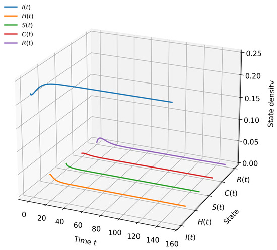
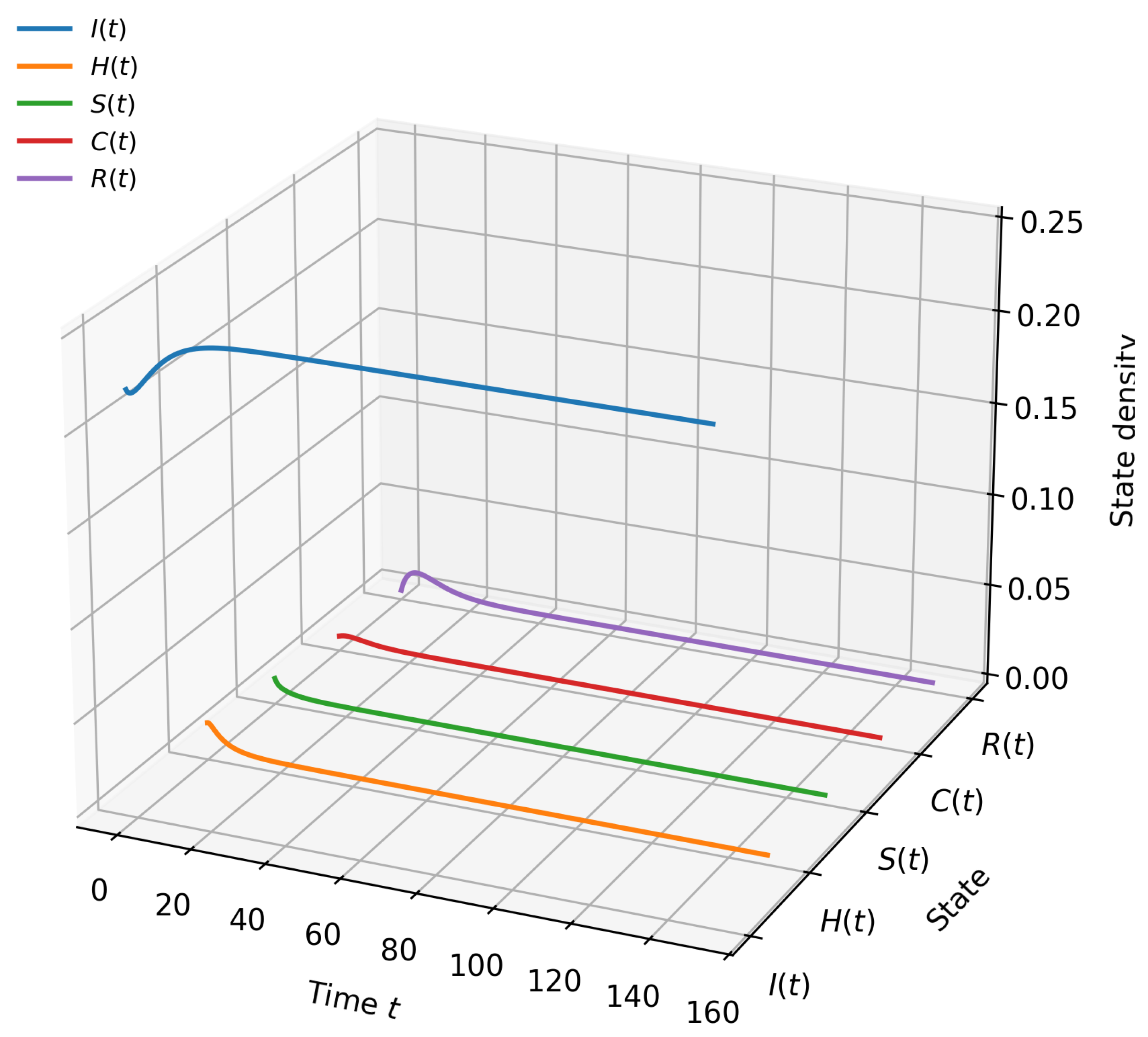
Using the $R_0<1$ setting in Table 2, we obtain $R_0\approx 0.56818$ and the information-free equilibrium $E_0=(0.25,0,0,0,0)$. Here, $\tau =0$ and the initial state is $(I,H,S,C,R)=(0.22,0.015,0.009,0.003,0)$. The beneficiary, spreader, and holder states $H\left(t\right)$, $S\left(t\right)$, and $C\left(t\right)$ decay to zero. The immune state $R\left(t\right)$ also vanishes, while $I\left(t\right)$ approaches $B/\mu =0.25$. The numerical result agrees with the zero-delay global stability result, and the corresponding trajectories are shown in Figure 2.

Figure 2. Numerical convergence to the information-free equilibrium for a parameter setting with $R_0<1$.

6.2. Numerical Verification of the Critical Behavioral Delay

For the stability-switching parameter set, $R_0=6.1184950338>1$ and

$$E^{*}=(1.892326607,2.270001454,1.449998824,1.239999644,3.147673471).$$

The reduced zero-delay characteristic polynomial has the four roots

$$-0.78138983,-0.18128493,-0.17725253\pm 0.14214255i,$$

while the independent R-direction eigenvalue is $-\mu =-0.1$. Thus, the five-dimensional equilibrium has five stable eigen-directions at zero delay, and the stability assumption used in Theorem 4 is satisfied.

The frequency equation has a unique positive real root and the associated phase calculation gives the compact threshold summary

$$z_0=0.01976290,{\omega }_0=0.140580594,{\theta }_0=2.079191973,{\tau }_0=14.790035485,$$

(69)

with ${\mathsf{\Phi }}^{\prime }\left(z_0\right)=0.001753231>0$. Thus, the critical conjugate pair crosses from the left half-plane to the right half-plane as $\tau$ increases through ${\tau }_0$.

As an independent spectral check, we solved the original characteristic Equation (28) directly in the complex plane at ${\tau }_0-0.01$, ${\tau }_0$, and ${\tau }_0+0.01$. Table 3 reports the two rightmost conjugate pairs. At ${\tau }_0$, only the critical pair reaches the imaginary axis, while the next pair remains separated from it by a real-part margin of about $0.0770$. The characteristic-equation residuals of the displayed roots are below $2\times {10}^{-16}$. Moreover, $|{\partial }_{\lambda }\mathsf{\Delta }(i{\omega }_0,{\tau }_0)|=0.1187244>0$, confirming that the critical pair is simple, and direct implicit differentiation gives

$$\mathrm{Re}{\left.\left({\displaystyle \frac{d\lambda }{d\tau }}\right)\right|}_{\tau ={\tau }_0}=0.002458159>0,$$

(70)

in agreement with the transversality result.

Table 3. Independent numerical verification of the rightmost characteristic roots around the first critical delay. The conjugates of the displayed roots are implicit.

Delay	Rightmost Pair	Next Rightmost Pair	Spectral Side
${\tau }_0-0.01$	$-2.4611\times {10}^{-5}\pm 0.1406504i$	$-0.0770830\pm 0.5587256i$	Stable
${\tau }_0$	$0\pm 0.140580594i$	$-0.0770116\pm 0.5583538i$	Critical
${\tau }_0+0.01$	$2.4552\times {10}^{-5}\pm 0.1405109i$	$-0.0769402\pm 0.5579825i$	Unstable

Using the normal-form construction in Section 4.3, the same critical point gives

$$c_1=-0.0053856024-0.0025880758i,{\mathcal{l}}_1=-0.0383097146<0.$$

(71)

Together with the positive crossing speed in Equation (70), this classifies the first Hopf bifurcation as supercritical: a small-amplitude periodic branch emerges for $\tau >{\tau }_0$ and is locally orbitally stable. This classification concerns the local branch near ${\tau }_0$ and does not imply stability of periodic behavior at arbitrarily large delays.

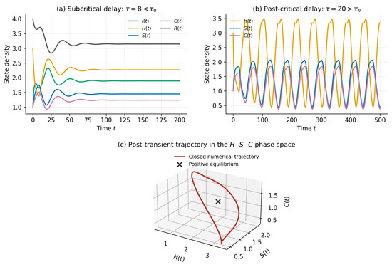
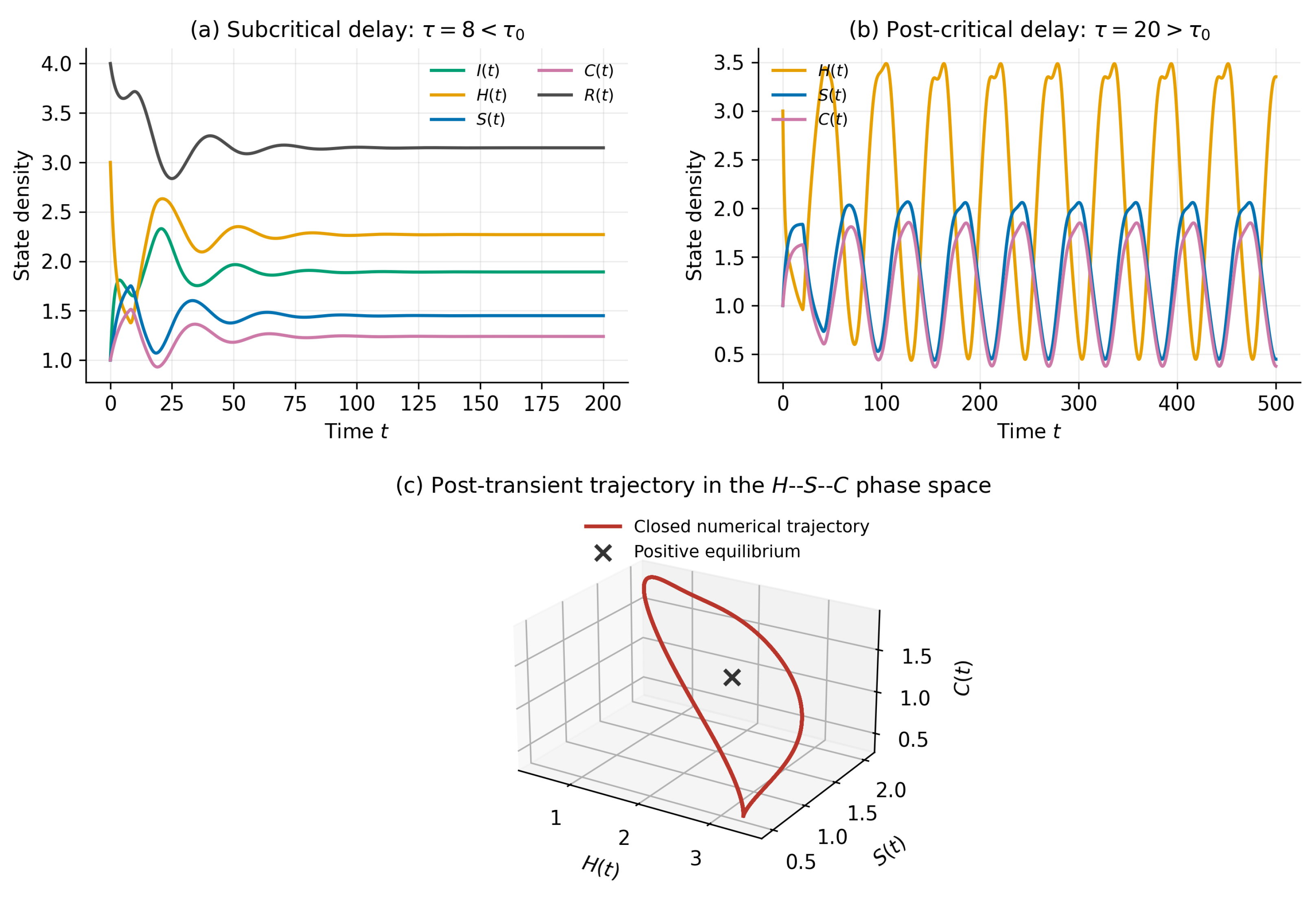
For the tested subcritical delay $\tau =8<{\tau }_0$, the five state variables exhibit damped oscillations and converge to $E^{*}$. At $T=500$, the population-balance residual is approximately $8.88\times {10}^{-15}$. For the tested post-critical delay $\tau =20>{\tau }_0$, the trajectory no longer converges to $E^{*}$. Sustained numerical oscillations are observed around the positive equilibrium over the simulated horizon. Over the post-transient interval $250\le t\le 500$, the peak-to-peak amplitude of $S\left(t\right)$ is approximately $1.6122$, the mean interval between the last consecutive peaks is approximately $57.65$, the minimum state value on $[0,500]$ is approximately $0.3690$, and the population-balance residual is approximately $1.60\times {10}^{-14}$. This observation supports the predicted loss of equilibrium stability for this parameter setting but should not be interpreted as a statement about all $\tau >{\tau }_0$. The corresponding trajectories and phase-space path are shown in Figure 3.

Figure 3. Delay-induced changes around the positive propagation equilibrium: (a) convergence for $\tau =8<{\tau }_0$ (the displayed interval is $0\le t\le 200$, while the simulation continues to $T=500$); (b) sustained numerical oscillations over the simulated horizon for $\tau =20>{\tau }_0$; and (c) the post-transient closed numerical trajectory in the H–S–C phase space.

For panel (c), the initial transient $t<250$ is discarded. The remaining trajectory forms a closed numerical path around $(H^{*},S^{*},C^{*})\approx (2.2700,1.4500,1.2400)$. The local normal-form calculation now identifies a stable periodic branch immediately to the right of ${\tau }_0$. Because the trajectory in panel (c) is computed at the much larger delay $\tau =20$, however, we continue to treat this particular closed path as finite-horizon numerical evidence rather than as a consequence of the local Hopf theorem.

6.3. Long-Transient Verification near the Critical Delay

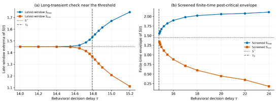
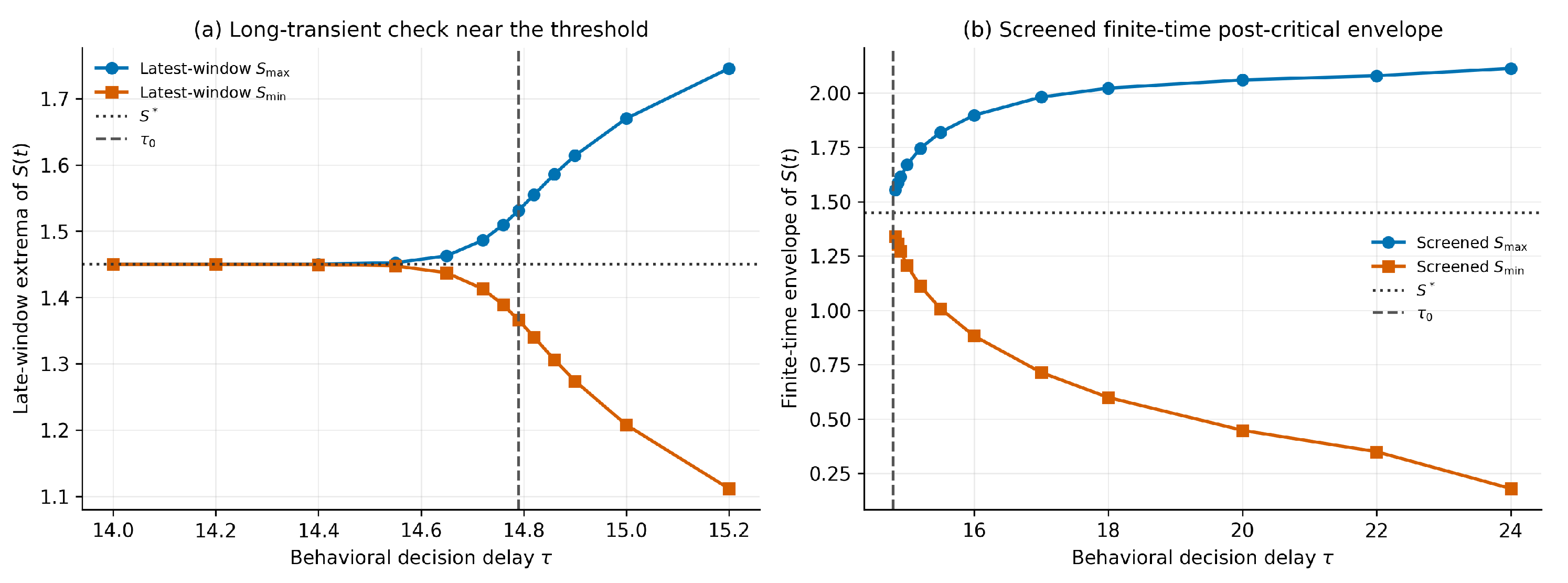
Near ${\tau }_0$, slowly decaying oscillations may persist for a long time. To reduce the risk of classifying a long transient as a post-critical periodic oscillation, each delay value close to ${\tau }_0$ is integrated to $T=8000$. The amplitudes of $S\left(t\right)$ in the last three consecutive windows of length 500 are compared. A point is included in the screened finite-time numerical envelope only when $\tau >{\tau }_0$, the terminal amplitude exceeds ${10}^{-3}$, and the change in amplitude between adjacent terminal windows is less than $3\%$. Define

$$S_{\max }\left(\tau \right)=\underset{T_{\mathrm{tr}}\le t\le T}{\max }S(t;\tau ),S_{\min }\left(\tau \right)=\underset{T_{\mathrm{tr}}\le t\le T}{\min }S(t;\tau ).$$

(72)

At $\tau =14.79<{\tau }_0$, visible oscillations remain over a long time interval but continue to decay slowly. The value $\tau =14.82>{\tau }_0$ is the first sampled post-critical delay satisfying the operational finite-time criterion. It remains a grid- and horizon-dependent numerical detection value rather than a replacement for the analytical threshold in Equation (69); the existence, direction, and local stability of the bifurcating periodic branch are instead determined by the normal-form calculation in Section 4.3 and Section 6.2.

The long-transient behavior near the critical delay is summarized in Figure 4.

Figure 4. Long-transient numerical verification near the critical behavioral decision delay: (a) late-window extrema of $S\left(t\right)$ near the analytical threshold, including slowly decaying subcritical oscillations; and (b) the screened finite-time post-critical envelope. The vertical dashed line marks ${\tau }_0=14.790035485$.

6.4. Effect of Behavioral Decision Delay

This subsection uses a different parameter set from the stability-switching example above. The earlier set is used to locate and check the first stability boundary near ${\tau }_0=14.790035485$. The delay/control set is used for the delay, average-degree, and control experiments. Its plotted range $0\le \tau \le 8$ stays below its own first stability boundary. Figure 5, Figure 6 and Figure 7 therefore compare transient delay effects, network-degree effects, and intervention performance inside a stable regime; they are not a second test of the first Hopf point.

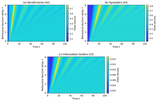
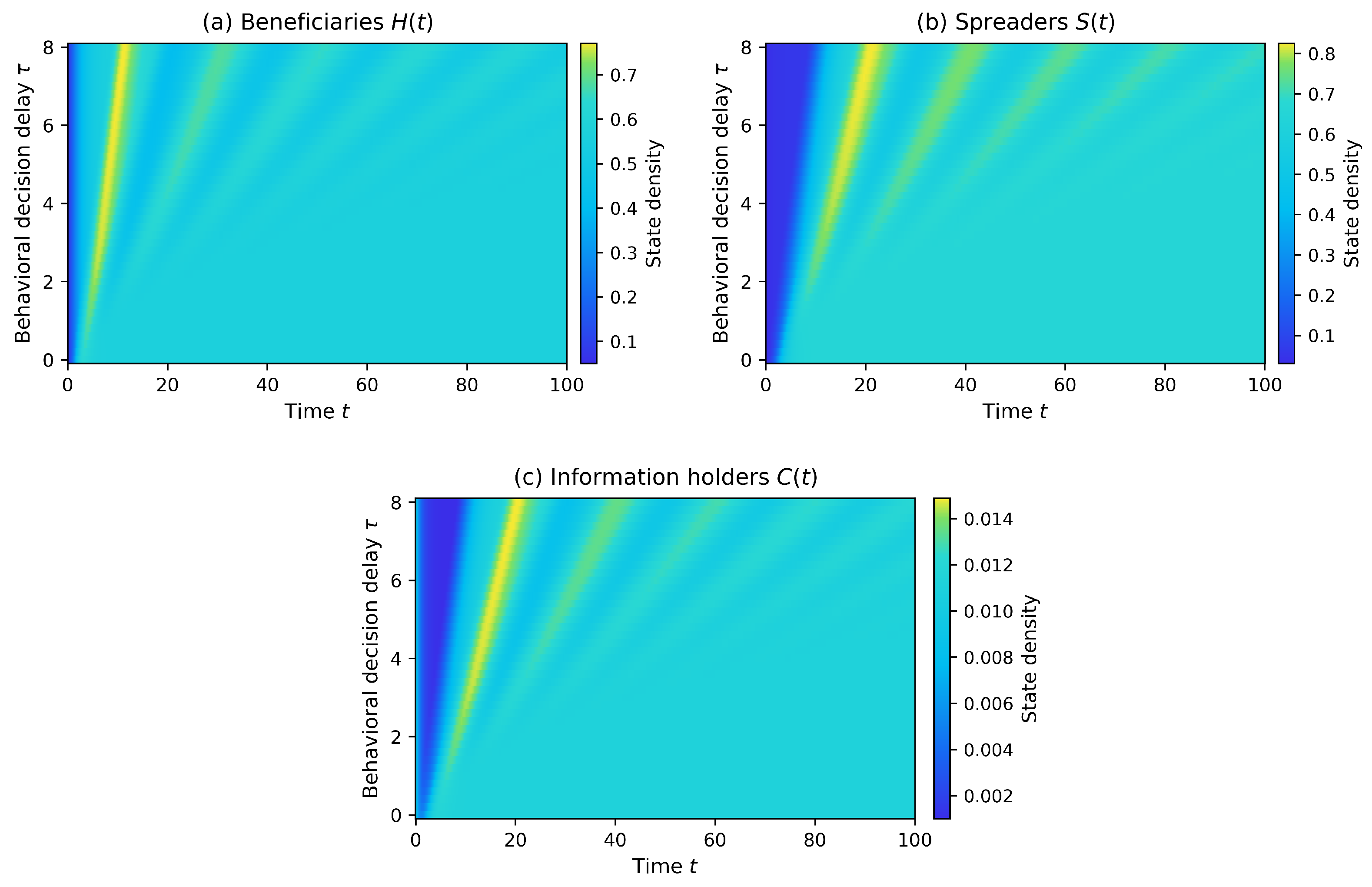
Figure 5. Two-dimensional delay–time heatmaps for (a) information beneficiaries, (b) spreaders, and (c) information holders. The delay range $0\le \tau \le 8$ lies below the first critical delay for this parameter set.

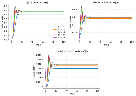
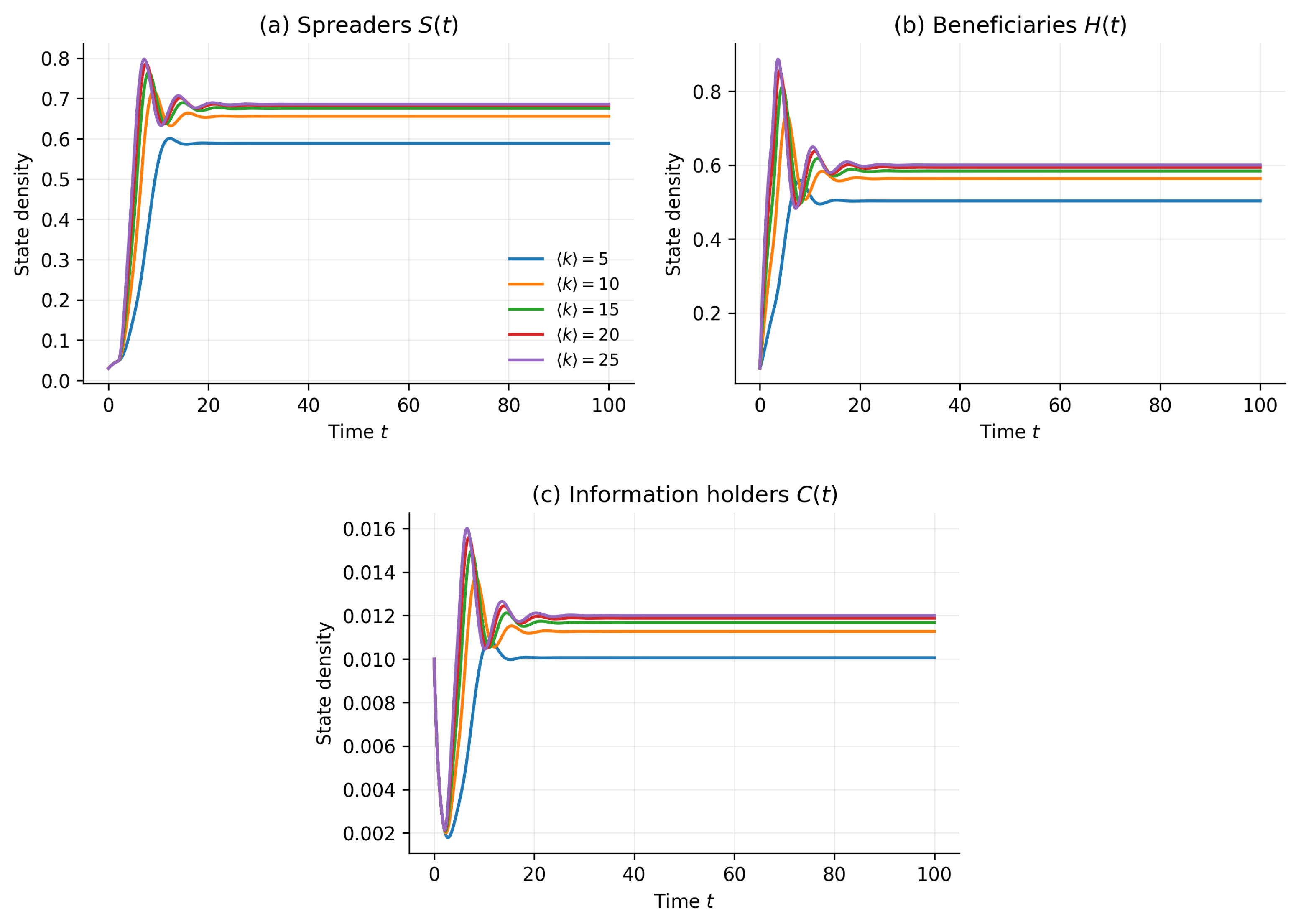
Figure 6. State trajectories under different average network degrees for $\tau =2$: (a) spreaders, (b) beneficiaries, and (c) information holders. The tested values are $⟨k⟩=5,10,15,20,25$.

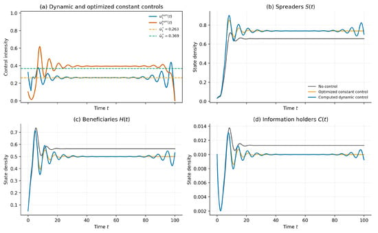
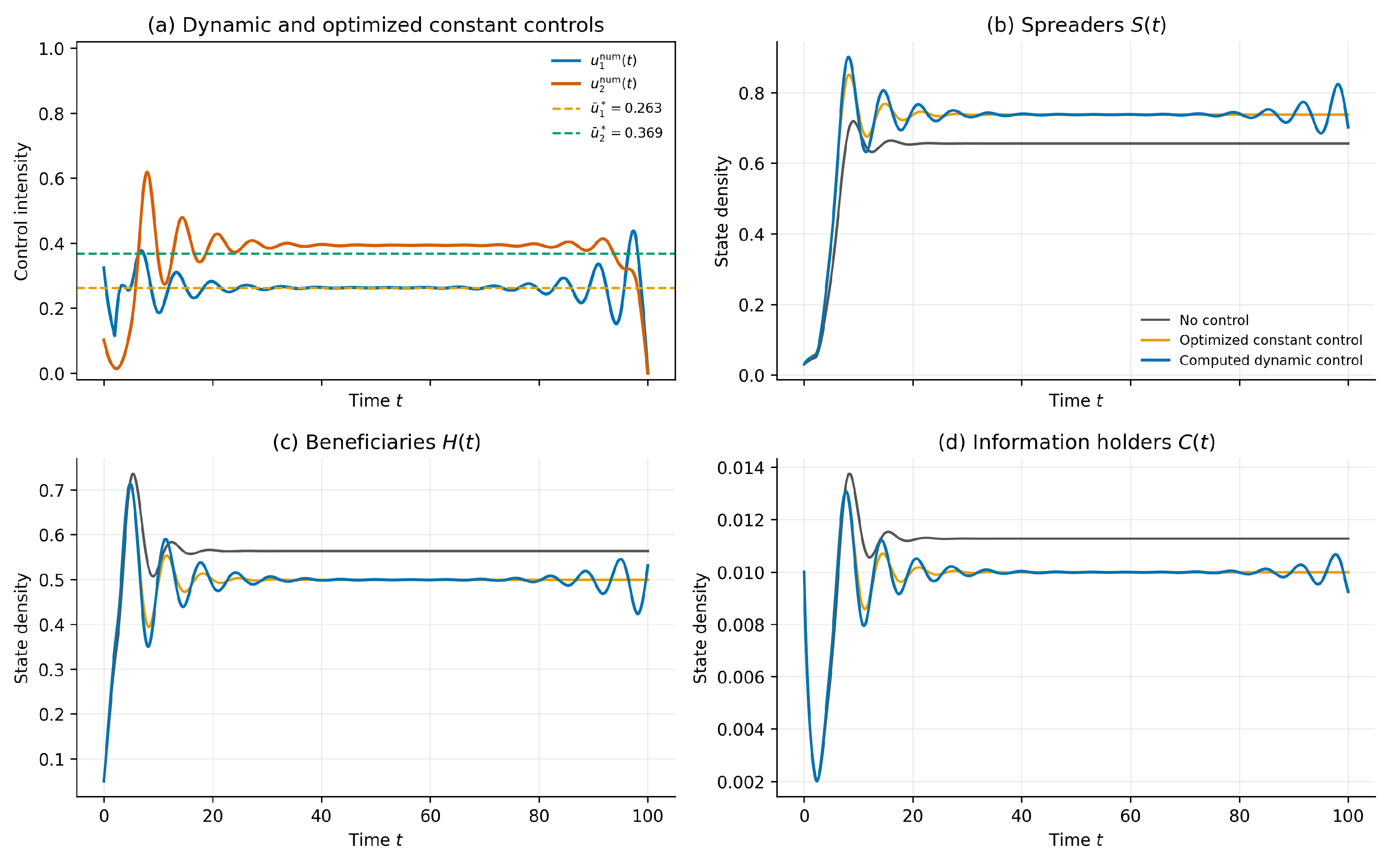
Figure 7. Control profiles and state comparisons: (a) computed dynamic controls and the numerically optimized constant intensities; (b) spreaders; (c) information beneficiaries; and (d) information holders under no control, optimized constant control, and computed dynamic control.

For the delay-effect simulations, we use the “Delay/control analysis” parameter set in Table 2. The constant history is $(I,H,S,C,R)=(0.90,0.05,0.03,0.01,0.01)$, and the delay is varied over $\tau =0,0.2,0.4,\dots ,8$. Each delay value is solved independently from the delayed model. As the behavioral decision delay increases, the transient peaks of $H\left(t\right)$, $S\left(t\right)$, and $C\left(t\right)$ generally occur later, and the adjustment process lasts longer. The delay does not change the equilibrium coordinates themselves; therefore, differences that remain near a finite terminal time for larger delays should be interpreted as incomplete transient decay rather than evidence of different long-term equilibria.

For this parameter set, the first effective critical delay from the analytical threshold procedure is about $27.7345$. Every delay in Figure 5 is therefore below the first stability boundary. Each horizontal row is an independent delayed simulation, and the color gives the state density at that time.

6.5. Effect of Average Network Degree

With the same delay/control parameter set in Table 2, we fix $\tau =2$ and vary $⟨k⟩=5,10,15,20,25$. Changes in the average degree alter the transient response, peak values, and equilibrium levels of $H\left(t\right)$, $S\left(t\right)$, and $C\left(t\right)$. Because $⟨k⟩$ enters both the propagation contact intensity $\kappa =\alpha ⟨k⟩$ and the holder-intervention intensity $q=\epsilon ⟨k⟩$, the displayed response represents their combined net effect for this parameter set and should not be interpreted as a universal monotonic network effect.

6.6. Numerical Optimal Control

For the optimal-control experiment, the delay/control parameter set in Table 2 is used with $\tau =2$, $T=100$, $c_1=1$, and $c_2=0.02$. Here, $c_1=1$ fixes the reference cost scale and $c_2=0.02$ is a baseline dimensionless weighting rather than an empirical cost estimate; sensitivity to the relative weight is examined below. We compare no control, a numerically optimized constant-control benchmark, and the computed dynamic control $(u_1^{\mathrm{num}}\left(t\right),u_2^{\mathrm{num}}\left(t\right))$ generated by the forward–backward optimality system. For the constant benchmark, the pair $({\overline{u}}_1,{\overline{u}}_2)\in {[0,1]}^2$ is held fixed over time and its objective is maximized numerically over the full box. A $0.01$ grid scan of the baseline box followed by bound-constrained local polishing gives

$$({\overline{u}}_1^{*},{\overline{u}}_2^{*})=(0.263107,0.369078),$$

(73)

with $J_{\mathrm{const}}=66.92739$.

With the reproducible settings stated above, the forward–backward iteration converges after 42 iterations. The final control-update error is $4.127\times {10}^{-8}$, the projection residual is $6.009\times {10}^{-8}$, the minimum state value is $m_{\min }=0.00200522$, and the population-balance error is $1.237\times {10}^{-11}$. The converged pair satisfies the reported first-order projection conditions numerically. Because global concavity of the full delayed control problem and uniqueness of its optimizer are not established, we treat this pair as a numerical candidate generated by the optimality system rather than as a proved unique or global maximizer.

We also ran the forward–backward sweep from different initial control guesses. At $\mathsf{\Delta }t=0.02$, zero and half-intensity guesses converged to the same displayed objective value, $J\approx 67.00103$. On a coarser grid, $\mathsf{\Delta }t=0.10$, the initial guesses $(0,0)$, $(0.5,0.5)$, and $(1,1)$ converged in 42, 40, and 46 iterations and all gave $J=67.000617$ to six decimal places. The largest pairwise difference between the final control profiles was below $1.8\times {10}^{-7}$, and the largest statewise difference was below $8.6\times {10}^{-8}$. This is a useful numerical robustness check, but it is not a proof of global uniqueness.

The computed dynamic controls satisfy

$$\begin{array}{cccc}\hfill \max u_1^{\mathrm{num}}& =0.437557,\hfill & \hfill \mathrm{mean}\left(u_1^{\mathrm{num}}\right)& =0.263084,\hfill \\ \hfill \max u_2^{\mathrm{num}}& =0.618238,\hfill & \hfill \mathrm{mean}\left(u_2^{\mathrm{num}}\right)& =0.369864.\hfill \end{array}$$

The optimized constant intensities in Equation (73) are very close to these dynamic-control means. Thus, the numerical advantage of the dynamic strategy is associated mainly with the timing of intervention rather than with a large change in average control intensity.

To distinguish propagation performance from intervention cost, define

$$G_S={\int }_0^{T}S\left(t\right)dt,C_u={\int }_0^T\left[{\displaystyle \frac{c_1}{2}}{u}_1^2\left(t\right)+{\displaystyle \frac{c_2}{2}}{u}_2^2\left(t\right)\right]dt,J=G_S-C_u.$$

(74)

The revised comparison is given in Table 4.

Table 4. Cumulative propagation benefit, control cost, and net objective value under the revised control benchmarks.

Strategy	${\mathit{G}}_{\mathit{S}}$	${\mathit{C}}_{\mathit{u}}$	J
No control	62.3891	0	62.3891
Optimized constant control	70.5249	3.5975	66.9274
Computed dynamic control	70.6904	3.6894	67.0010

The optimized constant benchmark is substantially stronger than the illustrative fixed pair used in the original submission. The dynamic candidate nevertheless retains a positive, although modest, net advantage:

$$J_{\mathrm{dynamic}}=67.0010>J_{\mathrm{const}}=66.9274>J_{\mathrm{no}}=62.3891.$$

(75)

The difference $J_{\mathrm{dynamic}}-J_{\mathrm{const}}=0.0736$ is about $0.11\%$ of the optimized constant objective. We therefore interpret the gain as a small timing benefit under the baseline cost structure rather than as a large dominance of time-varying control.

6.7. Sensitivity to Relative Control Costs

To test whether the dynamic-control comparison is driven by the relatively low baseline value $c_2=0.02$, we keep $c_1=1$ and vary $c_2$ from $0.01$ to 1. For every cost setting, the constant benchmark is re-optimized over $({\overline{u}}_1,{\overline{u}}_2)\in {[0,1]}^2$, and the dynamic forward–backward sweep is recomputed from the same history. Table 5 shows that the computed dynamic candidate has a slightly larger objective than the optimized constant benchmark throughout $1\le c_1/c_2\le 100$.

Table 5. Sensitivity of the optimized constant and computed dynamic control objectives to the relative control-cost weights, with $c_1=1$.

${\mathit{c}}_2$	${\mathit{c}}_1/{\mathit{c}}_2$	${\mathit{J}}_{\mathbf{const}}$	${\mathit{J}}_{\mathbf{dynamic}}$	${\mathit{J}}_{\mathbf{dynamic}}-{\mathit{J}}_{\mathbf{const}}$
0.01	100	67.06469	67.14725	0.08256
0.02	50	66.92739	67.00103	0.07364
0.05	20	66.84604	66.91429	0.06825
0.10	10	66.81909	66.88557	0.06648
0.20	5	66.80565	66.87125	0.06560
0.50	2	66.79759	66.86266	0.06507
1.00	1	66.79491	66.85980	0.06490

The response of the controls is also consistent with their cost interpretation. As $c_2$ increases from $0.01$ to 1, the mean dynamic intensity of $u_2$ decreases from approximately $0.7424$ to $0.00734$, while the mean of $u_1$ remains near $0.263$ because $c_1$ is fixed. Across all seven cost settings, the forward–backward sweep converges in 40–45 iterations, the final control-update error is below $4.9\times {10}^{-8}$, and the minimum state value remains above $0.0020052$. Thus, the baseline conclusion does not depend solely on assigning a very small cost to the second control; however, the improvement over the optimized constant benchmark remains quantitatively modest.

7. Sensitivity Analysis

Sensitivity of the First Critical Delay to Post-Benefit Behavioral Rates

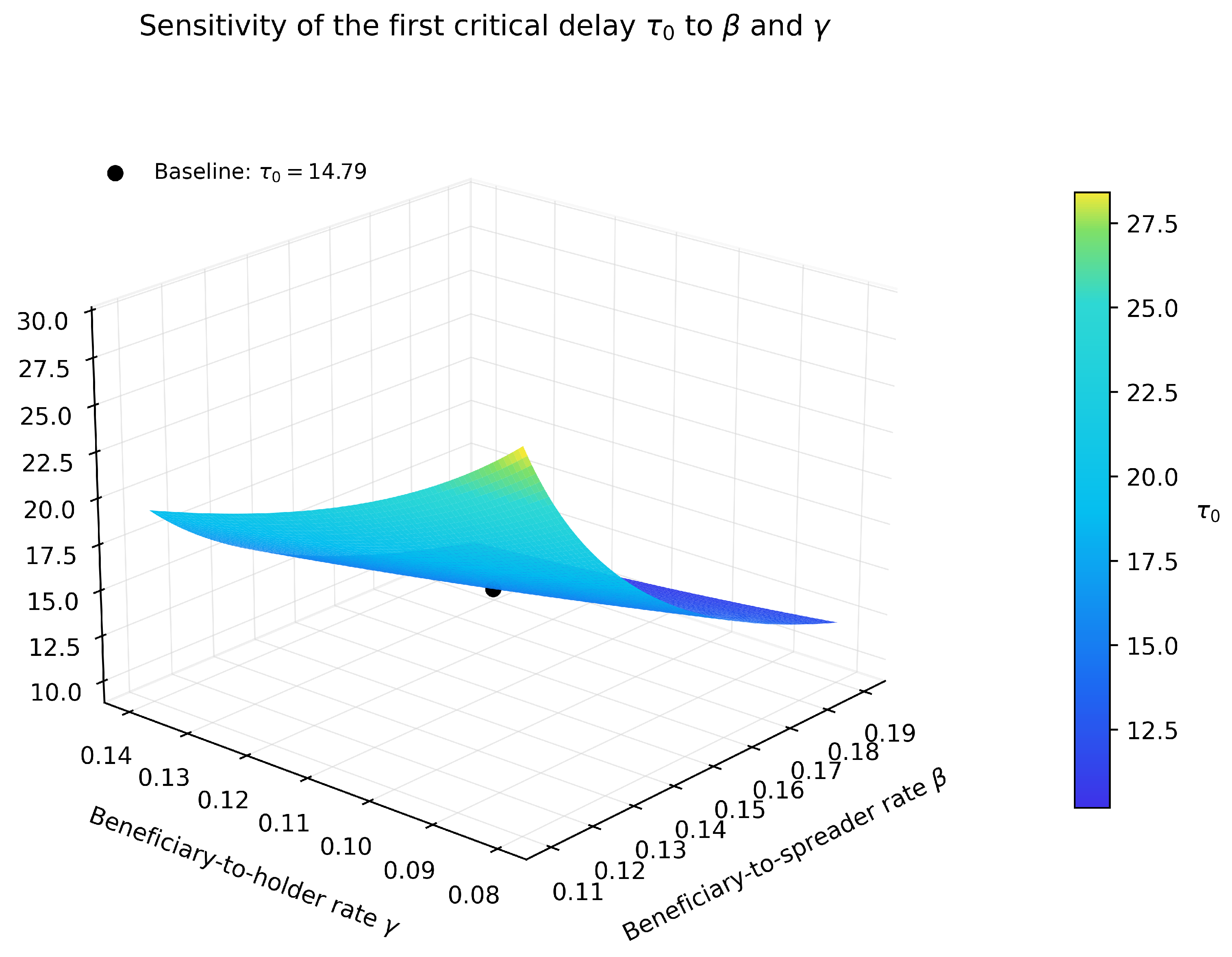
To see how the two post-benefit branching rates change the stability margin, we vary $\beta$ and $\gamma$ around the stability-switching parameter set in Table 2. The baseline is $({\beta }_0,{\gamma }_0)=(0.147915,0.109251)$ with ${\tau }_0=14.790035485$. We use $\beta \in [0.11,0.19]$ and $\gamma \in [0.08,0.14]$ and keep the other parameters fixed.

For each sampled pair $(\beta ,\gamma )$, we recompute the positive equilibrium and check its positivity and zero-delay Routh–Hurwitz conditions. We then solve Equation (38), recover the phase from Equation (44), and keep only critical delays that satisfy the original characteristic Equation (28). Each point in Figure 8 is calculated by the same threshold procedure used in Section 4. No curve fitting is used.

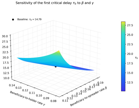
Figure 8. Three-dimensional sensitivity surface of the first critical behavioral decision delay ${\tau }_0$ with respect to the beneficiary-to-spreader rate $\beta$ and beneficiary-to-holder rate $\gamma$. The black marker denotes the baseline point $(\beta ,\gamma ,{\tau }_0)=(0.147915,0.109251,14.7900)$.

Every sampled pair gives a positive equilibrium, satisfies the zero-delay stability conditions, and produces a valid first critical delay. The calculated values of ${\tau }_0$ range from about $10.1547$ to $28.8032$. In this local window, ${\tau }_0$ falls as either $\beta$ or $\gamma$ increases with the other parameter fixed. Faster post-benefit transitions therefore leave a smaller delay margin before the first spectral stability switch for this parameter set. This pattern is local to the parameter range shown in Figure 8; we do not claim that it holds globally.

8. Conclusions

This paper starts from a simple behavioral fact: people who benefit from useful information do not always pass it on. The delayed IHSCR model separates this choice into two paths. A beneficiary may continue spreading the information or become an information holder. Holders may also discourage active spreaders. Information holding is therefore treated as its own behavioral state, not as an automatic continuation of the beneficiary process.

The basic reproduction number determines whether a positive propagation equilibrium exists. Its stability also depends on the system parameters and the behavioral delay. At zero delay, the positive equilibrium is locally asymptotically stable under the stated Routh–Hurwitz conditions. Using $\tau$ as the bifurcation parameter gives a transcendental characteristic equation and a frequency equation for imaginary roots. For the parameter set used in the stability-switching example, ${\omega }_0=0.140580594$ and ${\tau }_0=14.790035485$. Independent characteristic-root calculations verify that exactly one simple conjugate pair crosses the imaginary axis at this first critical point. The first Lyapunov coefficient is ${\mathcal{l}}_1=-0.0383097146<0$, so the local Hopf bifurcation is supercritical and its small-amplitude post-critical periodic branch is locally orbitally stable. The tested subcritical trajectory converges to the positive equilibrium. The tested post-critical trajectory shows sustained oscillations over the simulated horizon. Long simulations also reveal very slow decay close to ${\tau }_0$, so a short run can easily make a long transient look periodic. Average network degree affects both propagation and holder-mediated intervention, and its net effect depends on the parameter set. The sensitivity analysis adds another result: near the baseline point, the first critical delay falls as either $\beta$ or $\gamma$ increases.

The control problem acts on the two mechanisms linked to information holding. The first control promotes the transition from beneficiaries to spreaders. The second weakens holder-mediated suppression. Because the beneficiary state is delayed, the adjoint equation contains advanced terms at $t+\tau$. At the baseline cost weights, the computed dynamic candidate gives $J=67.0010$, compared with $66.9274$ for the numerically optimized constant control and $62.3891$ for no control. The dynamic advantage over the optimized constant benchmark is modest ($0.0736$ in the objective), and the optimized constant intensities are close to the dynamic-control means, indicating that the additional gain comes mainly from temporal reallocation. Repeating both optimizations over $1\le c_1/c_2\le 100$ preserves the same ordering while confirming that the magnitude of the gain depends on the relative control costs.

Benefiting from information and deciding to spread it are not the same step. The post-benefit branch is therefore more than an additional compartment: together with holder-mediated suppression, it creates a behavioral feedback loop whose decision delay can change equilibrium stability and whose two channels lead to a distinct delayed-control problem. It also has clear limits. Network structure is represented only through average degree. Because the delayed transitions are written as outflow rates, arbitrary nonnegative histories do not make the whole nonnegative cone invariant; the delayed results are stated for nonnegative-feasible trajectories. Lemma 1 shows that such histories exist near every positive equilibrium on any fixed finite interval, and the reported numerical trajectories remain strictly positive without truncation. The first Lyapunov coefficient resolves the local direction and orbital stability of the branch born at the first Hopf point, but we do not continue this branch globally or claim permanent instability for every $\tau >{\tau }_0$. Future work can use a positive-invariant maturation-delay formulation, move beyond the average-degree approximation, and study global and secondary bifurcations of the periodic branch. A further extension is to introduce explicit spatial coupling through a reaction–diffusion formulation and then examine whether local-activity concepts for spatially coupled nonlinear systems [32] provide useful criteria for the onset of complex propagation patterns.

References

- Wasko, M.M.; Faraj, S. Why Should I Share? Examining Social Capital and Knowledge Contribution in Electronic Networks of Practice. MIS Q. 2005, 29, 35–57. [Google Scholar] [CrossRef] [Scilit]
- Bock, G.W.; Zmud, R.W.; Kim, Y.G.; Lee, J.N. Behavioral Intention Formation in Knowledge Sharing: Examining the Roles of Extrinsic Motivators, Social-Psychological Forces, and Organizational Climate. MIS Q. 2005, 29, 87–111. [Google Scholar] [CrossRef] [Scilit]
- Kankanhalli, A.; Tan, B.C.Y.; Wei, K.K. Contributing Knowledge to Electronic Knowledge Repositories: An Empirical Investigation. MIS Q. 2005, 29, 113–143. [Google Scholar] [CrossRef] [Scilit]
- Haas, M.R.; Park, S. To Share or Not to Share? Professional Norms, Reference Groups, and Information Withholding Among Life Scientists. Organ. Sci. 2010, 21, 873–891. [Google Scholar] [CrossRef] [Scilit]
- Connelly, C.E.; Zweig, D.; Webster, J.; Trougakos, J.P. Knowledge Hiding in Organizations. J. Organ. Behav. 2012, 33, 64–88. [Google Scholar] [CrossRef] [Scilit]
- Černe, M.; Nerstad, C.G.L.; Dysvik, A.; Škerlavaj, M. What Goes Around Comes Around: Knowledge Hiding, Perceived Motivational Climate, and Creativity. Acad. Manag. J. 2014, 57, 172–192. [Google Scholar] [CrossRef] [Scilit]
- Evans, J.M.; Hendron, M.G.; Oldroyd, J.B. Withholding the Ace: The Individual- and Unit-Level Performance Effects of Self-Reported and Perceived Knowledge Hoarding. Organ. Sci. 2015, 26, 494–510. [Google Scholar] [CrossRef] [Scilit]
- Bogilović, S.; Černe, M.; Škerlavaj, M. Hiding behind a Mask? Cultural Intelligence, Knowledge Hiding, and Individual and Team Creativity. Eur. J. Work Organ. Psychol. 2017, 26, 710–723. [Google Scholar] [CrossRef] [Scilit]
- Daley, D.J.; Kendall, D.G. Epidemics and Rumours. Nature 1964, 204, 1118. [Google Scholar] [CrossRef] [Scilit] [PubMed]
- Zanette, D.H. Dynamics of Rumor Propagation on Small-World Networks. Phys. Rev. E 2002, 65, 041908. [Google Scholar] [CrossRef] [Scilit] [PubMed]
- Moreno, Y.; Nekovee, M.; Pacheco, A.F. Dynamics of Rumor Spreading in Complex Networks. Phys. Rev. E 2004, 69, 066130. [Google Scholar] [CrossRef] [Scilit] [PubMed]
- Huang, L.; Park, K.; Lai, Y.-C. Information Propagation on Modular Networks. Phys. Rev. E 2006, 73, 035103. [Google Scholar] [CrossRef] [Scilit] [PubMed]
- Nekovee, M.; Moreno, Y.; Bianconi, G.; Marsili, M. Theory of Rumour Spreading in Complex Social Networks. Phys. A 2007, 374, 457–470. [Google Scholar] [CrossRef] [Scilit]
- Kawachi, K.; Seki, M.; Yoshida, H.; Otake, Y.; Warashina, K.; Ueda, H. A Rumor Transmission Model with Various Contact Interactions. J. Theor. Biol. 2008, 253, 55–60. [Google Scholar] [CrossRef] [Scilit] [PubMed]
- Zhao, L.; Qiu, X.; Wang, X.; Wang, J. Rumor Spreading Model Considering Forgetting and Remembering Mechanisms in Inhomogeneous Networks. Phys. A 2013, 392, 987–994. [Google Scholar] [CrossRef] [Scilit]
- Cheng, J.-J.; Liu, Y.; Shen, B.; Yuan, W.-G. An Epidemic Model of Rumor Diffusion in Online Social Networks. Eur. Phys. J. B 2013, 86, 29. [Google Scholar] [CrossRef] [Scilit]
- Zhu, L.; Liu, M.; Li, Y. The Dynamics Analysis of a Rumor Propagation Model in Online Social Networks. Phys. A 2019, 520, 118–137. [Google Scholar] [CrossRef] [Scilit]
- Zhu, L.; Wang, B. Stability Analysis of a SAIR Rumor Spreading Model with Control Strategies in Online Social Networks. Inf. Sci. 2020, 526, 1–19. [Google Scholar] [CrossRef] [Scilit]
- Zhang, X.; Hu, Y.; Lu, S.; Guo, H.; Wei, X.; Li, J. Dynamic Analysis and Control of Online Information Dissemination Model Considering Information Beneficiaries. AIMS Math. 2025, 10, 4992–5020. [Google Scholar] [CrossRef] [Scilit]
- Li, C.; Ma, Z. Dynamic Analysis of a Spatial Diffusion Rumor Propagation Model with Delay. Adv. Differ. Equ. 2015, 2015, 364. [Google Scholar] [CrossRef] [Scilit]
- Li, C. A Study on Time-Delay Rumor Propagation Model with Saturated Control Function. Adv. Differ. Equ. 2017, 2017, 255. [Google Scholar] [CrossRef] [Scilit]
- Du, B.; Wang, H.; Liu, M. An Information Diffusion Model in Social Networks with Carrier Compartment and Delay. Nonlinear Anal. Model. Control 2018, 23, 568–582. [Google Scholar] [CrossRef] [Scilit]
- Wang, J.; Jiang, H.; Hu, C.; Yu, Z.; Li, J. Stability and Hopf Bifurcation Analysis of Multi-Lingual Rumor Spreading Model with Nonlinear Inhibition Mechanism. Chaos Solitons Fractals 2021, 153, 111464. [Google Scholar] [CrossRef] [Scilit]
- Ghosh, M.; Das, S.; Das, P. Dynamics and Control of Delayed Rumor Propagation through Social Networks. J. Appl. Math. Comput. 2022, 68, 3011–3040. [Google Scholar] [CrossRef] [Scilit] [PubMed]
- Cheng, Y.; Huo, L.; Zhao, L. Stability Analysis and Optimal Control of Rumor Spreading Model under Media Coverage Considering Time Delay and Pulse Vaccination. Chaos Solitons Fractals 2022, 157, 111931. [Google Scholar] [CrossRef] [Scilit]
- Dong, Y.; Huo, L.; Zhao, L. An Improved Two-Layer Model for Rumor Propagation Considering Time Delay and Event-Triggered Impulsive Control Strategy. Chaos Solitons Fractals 2022, 164, 112711. [Google Scholar] [CrossRef] [Scilit]
- Guo, H.; Yan, X.; Niu, Y.; Zhang, J. Dynamic Analysis of Rumor Propagation Model with Media Report and Time Delay on Social Networks. J. Appl. Math. Comput. 2023, 69, 2473–2502. [Google Scholar] [CrossRef] [Scilit] [PubMed]
- Luo, X.; Jiang, H.; Chen, S.; Li, J. Stability and Optimal Control for Delayed Rumor-Spreading Model with Nonlinear Incidence over Heterogeneous Networks. Chin. Phys. B 2023, 32, 058702. [Google Scholar] [CrossRef] [Scilit]
- Li, S.; Zhang, X.; An, Q. A Rumor Spreading Multi-Delay Model with Delay-Dependent Parameter. Math. Comput. Simul. 2024, 223, 34–49. [Google Scholar] [CrossRef] [Scilit]
- Yin, R.; Muhammadhaji, A. Dynamics in a Delayed Rumor Propagation Model with Logistic Growth and Saturation Incidence. AIMS Math. 2024, 9, 4962–4989. [Google Scholar] [CrossRef] [Scilit]
- Zhang, G.; Dong, H.; Li, H.; Xu, C.; Karimi, H.R.; Xiao, M.; Cao, J. Dynamics Mechanism of Time-Delay Reaction–Diffusion Rumor-Propagation Model with Saturation Control. Adv. Contin. Discret. Models 2025, 2025, 116. [Google Scholar] [CrossRef] [Scilit]
- Bucolo, M.; Fortuna, L.; Frasca, M.; Giudice, S. From Local Activity Lemma Beyond the Wave Computation Reaction–Diffusion CNN Based Networks. Int. J. Bifurc. Chaos 2006, 16, 411–417. [Google Scholar] [CrossRef] [Scilit]
- Huo, L.; Lin, T.; Fan, C.; Liu, C.; Zhao, J. Optimal Control of a Rumor Propagation Model with Latent Period in Emergency Event. Adv. Differ. Equ. 2015, 2015, 54. [Google Scholar] [CrossRef] [Scilit]
- Chen, S.; Jiang, H.; Li, L.; Li, J. Dynamical Behaviors and Optimal Control of Rumor Propagation Model with Saturation Incidence on Heterogeneous Networks. Chaos Solitons Fractals 2020, 140, 110206. [Google Scholar] [CrossRef] [Scilit]
- Li, C.; Ma, Z. Dynamics Analysis and Optimal Control for a Delayed Rumor-Spreading Model. Mathematics 2022, 10, 3455. [Google Scholar] [CrossRef] [Scilit]
- Yu, S.; Yu, Z.; Jiang, H. Stability, Hopf Bifurcation and Optimal Control of Multilingual Rumor-Spreading Model with Isolation Mechanism. Mathematics 2022, 10, 4556. [Google Scholar] [CrossRef] [Scilit]
- Yue, X.; Huo, L. Analysis of the Stability and Optimal Control Strategy for an ISCR Rumor Propagation Model with Saturated Incidence and Time Delay on a Scale-Free Network. Mathematics 2022, 10, 3900. [Google Scholar] [CrossRef] [Scilit]
- Ding, N.; Guan, G.; Shen, S.; Zhu, L. Dynamical Behaviors and Optimal Control of Delayed S2IS Rumor Propagation Model with Saturated Conversion Function over Complex Networks. Commun. Nonlinear Sci. Numer. Simul. 2024, 128, 107603. [Google Scholar] [CrossRef] [Scilit]
- Wang, H.; Kang, S.; Hu, Y. Dynamic Analysis and Optimal Control of Rumor Propagation Models Considering Different Education Levels and Hesitation Mechanisms. AIMS Math. 2024, 9, 20089–20117. [Google Scholar] [CrossRef] [Scilit]
- Liao, J.; Wang, J.; Li, J.; Jiang, X. The Dynamics and Control of a Multi-Lingual Rumor Propagation Model with Non-Smooth Inhibition Mechanism. Math. Biosci. Eng. 2024, 21, 5068–5091. [Google Scholar] [CrossRef] [Scilit] [PubMed]
- Hale, J.K.; Verduyn Lunel, S.M. Introduction to Functional Differential Equations; Springer: New York, NY, USA, 1993; Volume 99. [Google Scholar] [CrossRef] [Scilit]
- van den Driessche, P.; Watmough, J. Reproduction Numbers and Sub-Threshold Endemic Equilibria for Compartmental Models of Disease Transmission. Math. Biosci. 2002, 180, 29–48. [Google Scholar] [CrossRef] [Scilit] [PubMed]
- Hassard, B.D.; Kazarinoff, N.D.; Wan, Y.-H. Theory and Applications of Hopf Bifurcation; Cambridge University Press: Cambridge, UK, 1981; Volume 41. [Google Scholar]
- Göllmann, L.; Kern, D.; Maurer, H. Optimal Control Problems with Delays in State and Control Variables Subject to Mixed Control–State Constraints. Optim. Control Appl. Methods 2009, 30, 341–365. [Google Scholar] [CrossRef] [Scilit]
Disclaimer/Publisher’s Note: The statements, opinions and data contained in all publications are solely those of the individual author(s) and contributor(s) and not of MDPI and/or the editor(s). MDPI and/or the editor(s) disclaim responsibility for any injury to people or property resulting from any ideas, methods, instructions or products referred to in the content. |
© 2026 by the authors. Licensee MDPI, Basel, Switzerland. This article is an open access article distributed under the terms and conditions of the Creative Commons Attribution (CC BY) license.