


Abstract
Physics-informed neural networks (PINNs) approximate partial differential equations (PDEs) by enforcing governing equations and boundary conditions during training, but their accuracy depends on how collocation points are distributed and updated. We propose spatiotemporal compositional active sampling (STCAS), a reference-assisted offline configuration procedure that uses an analytic or high-accuracy numerical solution to rank complete three-stage sampling plans. It screens eight fixed rules, forms a task-specific shortlist, and evaluates bounded fixed, switched, and locally blended plans with independent selection sets and a composition guard. A safety-anchor decision retains the standard PINN unless the selected candidate is at least 5% better. Across five evaluations on 18 analytically specified two-dimensional Poisson tasks, this protocol improves 16 task means and ties two, reducing aggregate relative- error by 12.8% (hierarchical-bootstrap 95% interval ; one-sided paired Wilcoxon ). Against the confirmed fixed plan, aggregate error decreases by 8.2%. In comparison experiments designed for two transfer tasks and matched for main PINN training budgets, STCAS achieves the lowest aggregate mean reported error among the compared methods for both a steady convection–diffusion equation and a nonlinear time-dependent Burgers equation; its offline search cost is additional.
Keywords:
physics-informed neural networks; partial differential equations; active sampling; sampling plans; algorithm selection; stage-wise sampling MSC:
68T07
1. Introduction
Physics-informed neural networks (PINNs) embed differential equations and boundary conditions in the training objective of a neural network [1,2]. They approximate a continuous solution without a labeled dataset or a problem-specific mesh, and the same formulation accommodates sparse observations for forward, inverse, and data-assimilation problems [3,4]. When physical equations and limited measurements must be used together, PINNs serve as a useful complement to established numerical solvers.
Mesh-free training does not, however, remove the need to choose where the equation is enforced. A PINN evaluates its residual at a finite set of collocation points. Points placed in informative regions supply effective physical constraints; points that miss a narrow layer, a local source, or a boundary-adjacent feature may leave that structure poorly resolved. This sampling effect interacts with familiar optimization difficulties, including imbalance between loss gradients [5] and unequal convergence rates of solution components [6]. Consequently, even with a fixed network and optimizer, the placement and updating of collocation points can materially affect the final solution.
Existing sampling methods target different objectives but are typically designed as self-contained update policies. Residual-based adaptive refinement (RAR and RAD) adds or redistributes points according to the current equation residual [7]. Failure-informed sampling estimates where a prescribed accuracy condition is violated [8]. Importance sampling adjusts the probability of drawing candidate points [9], whereas R3 retains difficult points while resampling and releasing others [10]. None of these methods directly addresses the problem studied here: selecting a complete schedule in which one rule provides broad initial coverage, another concentrates on errors that emerge later, and two complementary proposals are combined when both remain useful.
Our previous work used source-field geometry for a related task-level choice [11]. It routed unambiguous instances to one expert sampler; ambiguous instances triggered a short greedy probe that selected the next rule from the current training state. That method was designed for low online overhead: it neither evaluated complete future schedules before making a stage decision nor constructed weighted point-set mixtures from two rules. The present study asks a different question: once several useful rules are available, can a bounded search over fully specified multi-stage plans find combinations that a fixed rule or a local stage-by-stage decision would miss?
To address this question, we propose spatiotemporal compositional active sampling (STCAS). The method divides training into three stages, measures eight fixed plans, retains the three strongest directly composable rules, and uses them to build complete plans through two operations: switching from one rule to another at a stage boundary, and blending the point proposals of two rules. Every candidate plan specifies its initial rule and both subsequent updates before training begins, so candidates are compared as complete plans rather than isolated one-step choices. STCAS is an offline configuration procedure: candidate ranking requires an analytic or high-accuracy numerical reference solution, rather than a reference-free online decision signal.
The term spatiotemporal carries a specific operational meaning throughout this paper. The spatial decision governs the distribution of collocation points over the PDE domain; the temporal decision specifies the training-stage boundary at which that distribution is kept, replaced, or blended. Neither term refers to a new physical representation of space–time PDEs. The methodological contribution is the bounded, non-greedy construction and evaluation of complete stage-wise sampling plans.
Contributions
- Formulating sampling-strategy selection as a complete-plan optimization problem. Existing adaptive samplers make local update decisions step by step; STCAS instead places the initial point distribution, stage transitions, and rule blending in one searchable three-stage plan space, enabling the construction and comparison of globally non-greedy schedules.
- A prospective evaluation protocol with dual-threshold protection. The method introduces six disjoint measurement sets and two hard 5% thresholds that statistically isolate candidate search from final reporting. The complete protocol independently re-verifies the selected plan before adoption and falls back to the standard PINN when the candidate does not clear the acceptance threshold; the primary comparison improves 16 task means and ties two.
- Transfer verification across equation types. The plan construction designed on a Poisson task family is applied to two structurally different equations—a two-dimensional steady convection–diffusion equation and the nonlinear time-dependent Burgers equation—and attains a lower mean reported error than every comparator on both, indicating that spatiotemporal compositional plan search is not confined to a single equation family.
2. Related Work
2.1. PINN Approximation and Training
PINNs approximate a solution by minimizing equation and boundary residuals computed through automatic differentiation [1,2]. Research has extended this formulation along several axes. Variational and domain-decomposed formulations improve locality and interface treatment [12,13]; gradient-enhanced training incorporates derivatives of the residual [14]; and physics-informed inversion combines equations with sparse observations [15]. These approaches modify the solver, the loss, or the information supplied to training. The present work holds the network, optimizer, and loss form fixed and studies only how collocation points are organized over the training run.
2.2. Adaptive Collocation
RAR and RAD use residual magnitude to locate regions that the current model satisfies poorly [7]. Their strength lies in a direct, inexpensive error indicator; however, residual magnitude can favor already visible errors and does not determine whether a different sampling mechanism should take over later. Failure-informed sampling estimates a failure region relative to a prescribed tolerance [8]; it supplies a probabilistic target but still defines a single update policy. Importance sampling reweights the draw toward informative candidates [9], and self-adaptive PINNs learn weights on difficult constraints rather than a sequence of sampling rules [16]. R3 mitigates propagation failure by retaining difficult points and refreshing the remainder [10]. Sobol sampling occupies the opposite, coverage-oriented end of the spectrum and spreads points with a low-discrepancy sequence [17]. STCAS does not replace these sampling ideas. It treats rule-induced point distributions as components and asks how a small number of them should be ordered or blended over a complete run.
2.3. Relation to Our Previous Routing Method
Table 1 states the overlap and differences directly. Both studies use a three-stage PINN setting and a pool of reusable sampling rules. The earlier method makes a low-cost routing decision from source geometry and, for ambiguous cases, selects the next rule through a short greedy probe. STCAS replaces that router with measured fixed-plan ranking, specifies both future updates before candidate training, evaluates complete plans, and adds pairwise point-set blending. Two diagnostic methods from the rule bank can still enter the fixed-plan screen, but they are not decomposed into switching or blending components. The new contribution is a complete-plan construction and bounded look-ahead, not the first use of stages or sampling-rule selection in PINNs.
Table 1.
Direct comparison with our previous geometry-aware routing method [11].
2.4. Algorithm Selection and Component Search
Algorithm selection studies how instance features can guide the choice among competing procedures [18,19], and ASlib provides standardized data for evaluating such choices [20]. Hyper-heuristics organize search over reusable heuristic components [21]. STCAS adopts this general perspective at the level of a PINN training plan: the candidate is not a rule name but a complete sequence of point-set operations. Its search space is deliberately restricted by measured fixed-rule performance and a small composition grammar.
3. Method
The goal of STCAS (spatiotemporal compositional active sampling) is to automatically find a good arrangement of training points for a physics-informed neural network (PINN), so that the network approximates the solution of a partial differential equation (PDE) more accurately.
Training a PINN requires placing a set of collocation points inside the equation’s domain—these are the locations where the network evaluates the equation residual and updates its parameters. Different sampling rules produce different point arrangements: for example, spreading points uniformly, concentrating them where the equation error is currently large, or mixing these strategies in fixed proportions. This paper defines eight such rules (listed in Table 2, Section 3.2); six of them can be freely combined, and the remaining two are used only in isolation.
Table 2.
The eight base methods and how STCAS uses them.
A sampling plan is a complete schedule that specifies, for each of three training stages (each lasting 120 parameter updates), which rule generates or replaces the collocation points. Every plan is fully determined before its training begins.
STCAS works in five steps:
- Prepare the PDE, the PINN architecture, and six mutually disjoint sets of measurement points (each reserved for a different evaluation purpose; see below).
- Run each of the eight rules alone for all three stages, producing eight fixed plans. Measure their errors and rank the six combinable rules; the top three are called .
- Combine by switching (use different rules at different stages) and blending (mix points from two rules at a stage boundary) to form 132 new plans. Together with the eight fixed plans, this yields 140 candidates.
- Execute the 132 new plans one by one, measure each error, and obtain a complete ranking of all 140 plans.
- Select a small group of top-performing plans and rerun them on C to verify stability. Use G to choose between the best composed and fixed plans, then use H to compare the frozen candidate with the uniform-point baseline. Only after both decisions are frozen does STCAS report the result on the unused set U.
Figure 1 illustrates the construction in Steps 2–3. Algorithm 1 gives the full five-step procedure in execution order. In the figure, “Keep-Points” means carrying the current point set into the next stage without replacement; it is an update choice, not a separate sampling rule. The following subsections describe each step in detail.
| Algorithm 1 Complete six-set STCAS procedure used in the Poisson study. |
|
Figure 1.
Construction of the STCAS candidate plans (Steps 2–3). “Exact Anchors” denotes the measured errors of fixed plans, and “Keep-Points” carries the current point set into the next stage. The label “same budget” refers to the paired final models, which share the same main-network training budget; it does not include the offline search cost. The stability verification, 5% threshold checks, comparison with the standard PINN, and final reporting in Step 5 are given in Section 3.5 and Algorithm 1.
3.1. Step 1: Prepare the PDE, PINN, and Six Measurement Sets
We consider a two-dimensional Poisson equation on ,
where identifies the task. The PINN is trained using only the forcing term and the boundary condition; no analytic solution enters the training loss:
Here, contains the interior collocation points, and contains the boundary points. The coefficient 10 is a fixed loss-balancing weight for the exact Dirichlet condition, chosen by prior agreement rather than tuned for STCAS alone. Because the PDE-residual and boundary losses can differ in numerical scale and convergence rate, the explicit weight keeps the boundary condition active during optimization. We fix this value before comparing sampling plans and apply it identically to every task and method; STCAS does not tune it. Supplementary experiments also tested weights 1, 5, and 20.
How is arranged across —which regions receive more points and which receive fewer—is what STCAS selects. The analytic solution (or reference solution) serves two purposes in this paper, neither of which enters the training loss:
- Generating the forcing term. For the Poisson tasks, an analytic solution is defined first, and the forcing term is obtained by automatic differentiation: . During training, the PINN sees only and the boundary condition; it never accesses . In a real application, is simply the known right-hand side of the PDE, and no analytic solution needs to be constructed.
- Measuring true accuracy. After training, the difference between the network prediction and the reference solution quantifies how good each plan actually is. STCAS uses this error on V/C/G/H during offline plan selection, and the final paper results are also reported on U using the same error—both rely on the reference solution.
STCAS is therefore a reference-solution-assisted offline configuration method: it relies on the reference solution to choose a plan, but the PINN training itself, once a plan is selected, does not require it. For the Burgers experiment, where no closed-form analytic solution exists, a high-resolution numerical reference solution is used in place of .
Specifically, the relative error on a measurement set A is
Smaller indicates a more accurate solution. STCAS uses six mutually disjoint measurement sets (each containing 4096 scrambled Sobol points) for the evaluations in the five steps above. Their roles are as follows: V (screening set) ranks all 140 plans in Step 4 and also supplies any diagnostic measurements during training. C (confirmation set) reruns the top few candidates multiple times in Step 5. G (guard set) checks whether the confirmed best combined plan truly outperforms the best fixed plan by at least 5%; if not, the fixed plan is kept. T (auxiliary reporting set) records ablation, external-baseline, candidate-budget, and sensitivity results after the candidate identity is frozen, but no value from T enters a per-pair model-selection calculation. H (safety set) compares the frozen STCAS candidate against the standard PINN (defined here as one fixed uniform collocation set throughout training); a candidate that is already a standard PINN is recorded as shared, whereas a nonuniform candidate falls back to the standard PINN if its advantage is less than 5%. U (primary reporting set) provides the final fresh test points, opened only after all decisions above have been frozen, so the reported error cannot change the selected plan.
The sets V and T are the disjoint even and odd subsequences of a Sobol stream pre-specified and hash-frozen before evaluation (seed and offsets documented in Appendix E). STCAS uses the analytic solution to evaluate errors of different plans and thereby select a good plan offline, but the analytic solution never appears as a training target in the loss function. The follow-up was pre-specified and hash-frozen before evaluation after the auxiliary comparison on T had been completed; the aggregate T result motivated this follow-up, but no T value was used to choose a model within any task–repetition pair. The separation of H from U ensures that the test points used for the primary reported error have never been consulted in any selection decision.
3.2. Step 2: Run the Eight Base Methods as Fixed Plans
The eight sampling rules are listed in Table 2. Every plan maintains 384 collocation points; at an update boundary, each rule retains or replaces points according to its definition. The standard PINN baseline retains one uniformly generated point set throughout training. RAD concentrates points at large-residual locations, the fixed-budget R3-style rule keeps difficult current points while replacing the rest, and the scheduled rules apply fixed proportions of retained and newly proposed points. The Sobol variants of certain rules generate candidate points from low-discrepancy Sobol sequences (rather than independent random samples), yielding more uniform spatial coverage.
The short label “R3” in the figures and tables denotes the fixed-budget variant defined in Appendix A, not the published standard R3 algorithm. The difference is how often points are replaced: the published R3 replaces points after every training step, whereas our variant replaces them only at the two stage boundaries. The reason for this change is that a STCAS plan is assembled from three stages, and all rules must replace points at the same moments before they can be placed in the same switching or blending plan for comparison; if R3 replaced points at every step, it could not be combined with the other rules. The published original R3 is run separately as an external baseline in Section 4, where the two versions are compared.
Six methods return a point set directly and can therefore be placed inside a new switching or blending plan. The two diagnostic methods contain their own internal probe-and-select procedure, so STCAS evaluates them as complete fixed plans but does not decompose them for later composition. Appendix A gives the numerical update rule for every method. These eight methods form the internal rule bank; comparisons with published external sampling algorithms are defined separately in Section 4.
All eight fixed plans train their main PINN for 360 Adam updates. Two of the eight rules are “diagnostic” (see Table 2): they must first discover which regions have large errors before choosing points. They do this by copying the current network, trial-training the copy for a few steps to expose high-error regions, then selecting points based on the result; the copy is discarded and the main network is unaffected. These trial steps are not counted toward the main network’s 360 updates, but they do consume additional computation and are therefore listed separately in the cost analysis.
Each base method is first run as one complete fixed plan. After the third training stage, its error is measured on V. The same measurements rank the six directly usable rules; their three best members are denoted by , in that order. This ranking is performed once for the current task and is not repeated inside a candidate plan.
The eight fixed-plan errors are carried into the ranking directly and are not rerun while the 132 composed plans are evaluated. After all 140 plans are ranked, the two lowest-error fixed plans advance to the independent verification step in Section 3.5, where several repeated runs determine the final fixed comparator, rather than relying on a single error on V.
3.3. Step 3: Build a Bounded Candidate Set from the Shortlist
The output of Step 2 is the ordered shortlist . STCAS expands this shortlist into complete three-stage plans. It does not re-rank the top three rules after a stage begins.
3.3.1. Stage-Switching Plans
Write a switching plan as . The first entry creates the initial point set, is applied after 120 Adam updates, and is applied after another 120 updates. We allow and . For example, first creates points with , replaces them with the set proposed by after Stage 1, and carries that set unchanged from Stage 2 into Stage 3. There are such plans. The position of an entry states exactly when its spatial distribution is used.
Rules that require a trained residual cannot apply residual-based selection before Stage 1. When such a rule appears as , it uses the warm-start generator specified in Appendix A: a pseudorandom uniform set for the random-backed rules or a scrambled Sobol set for Schedule-B Sobol. The entry determines only this initial set; at each later boundary, the rule generates points using its own fixed random seed (derived from the plan seed), ensuring exact reproducibility.
3.3.2. Local-Blending Plans
A blending plan pairs the leading composable rule with either or , that is, the two pairings are and . Given a pairing, the initial point set is created by one member of the pair: for example, in the pair , either or may generate the starting points (2 choices). At each later boundary, both rules propose 384 points. The plan keeps a proportion from and fills the remainder from the other rule. Thus, gives 288 points from and 96 from its partner. The grid ranges from an equal mixture to a conservative modification of the best directly composable fixed rule. The two boundaries choose their weights independently (5 choices each), so this balance may change between Stages 2 and 3. In total, we have 2 (pairings) (initial choices) (first-boundary weights) (second-boundary weights) plans.
3.3.3. Bounded Plan Set
The eight measured fixed plans remain candidates. Adding the 32 switching plans and 100 blending plans yields 140 complete plans for the current task.
The reduction is substantial. Applying the same grammar to all six directly composable rules would produce
plans: six initial choices and six rules plus “keep” at each later switching stage, together with every rule pair for blending. The shortlist and pair restrictions contract this family to 140 plans, an 86.7% reduction before composed-plan evaluation. Of these, the eight fixed plans have already been evaluated in Step 2; Step 4 evaluates only the 132 newly constructed plans.
Table 3 summarizes the bounded construction of the complete candidate set.
Table 3.
Bounded construction of the plan set for one task after shortlisting.
At this point, every plan is fully specified. No rule ranking or shortlist construction occurs while that plan is being trained.
3.4. Step 4: Evaluate the 132 New Plans
The eight fixed plans already carry their errors from Step 2. Each of the 132 new plans is executed in the same sequence:
- Apply its initial rule to create 384 interior collocation points, then train the PINN for 120 Adam updates.
- Apply its first point-set operation, then train for another 120 updates.
- Apply its second point-set operation, train for the final 120 updates, and record the resulting error on V.
One plan therefore always contains 360 Adam updates. The network and optimizer remain unchanged; plans differ only in the point distributions applied at the three stages and in the boundaries at which those distributions change.
For a blending update with weight , contributes points and its partner contributes , with restricted to . Duplicate coordinates are identified after rounding to four decimal places; the original coordinates from the first occurrence are retained.
Point selection from the two proposals is deterministic once the plan seed s is fixed. Appendix E documents the numerical details; offsets ensure reproducibility and prevent cross-proposal duplicates from leaving gaps.
3.5. Step 5: Verify Stability, Check Against the Baseline, and Report
The first four steps produce errors on the screening set V for all 140 plans. A single run’s lowest error may be due to luck, so Step 5 verifies candidate stability and applies two thresholds to guard against false selection.
3.5.1. Select Confirmation Candidates
STCAS picks 6 plans for confirmation: the 2 lowest-error fixed plans on V, plus 4 lowest-error composed plans (excluding switching plans that reproduce a fixed rule; if both switching and blending types exist, at least one of each is kept).
3.5.2. Confirm Stability via Repeated Runs
Each of the 6 candidates is run 4 more times and measured on the confirmation set C. For candidate c, let and be the sample mean and standard deviation of its four errors. The stability score is
Adding the standard deviation penalizes variability: even if a plan has low mean error, unstable results worsen its score. The fixed candidate with the lowest becomes (best fixed plan), and the composed candidate with the lowest becomes (best composed plan).
3.5.3. First Threshold: Is the Composed Plan Really Better than the Fixed Plan?
Retrain and from the same new seed , and compare on the guard set G:
Meaning: the factor 100 converts the dimensionless error ratio to a percentage, so the threshold 5 requires a 5% relative improvement; must outperform by at least 5% to be accepted. If the margin is smaller, STCAS retains the fixed plan . This threshold prevents accepting a composed plan whose advantage is small and may be noise, a risk when 140 candidates have been tested.
3.5.4. Frozen Candidate and Auxiliary Recording
The threshold check produces a frozen STCAS candidate (either or ). Its error and the internal fixed comparator’s error may be recorded on the auxiliary set T for ablation analysis, but T values do not influence any subsequent decision.
3.5.5. Second Threshold: Is the Frozen Candidate Really Better than the Standard PINN?
If is already the standard uniform plan (i.e., it is the standard PINN), the pair shares one model, and no further comparison is needed. Otherwise, retrain and the standard PINN from the same initialization, and compare on the safety-anchor set H:
Same meaning: the factor 100 converts the dimensionless error ratio to a percentage, so the threshold 5 requires a 5% relative improvement; must beat the standard PINN by at least 5% to be retained; otherwise, the standard PINN is selected. Once made, this decision is never revisited.
3.5.6. Final Reporting
Only after the decision is frozen are the selected model and the standard PINN evaluated on the fresh reporting set U. Because U is not used until after the decision, its results cannot change the selected plan—this guarantees honest reporting. When both entries are the same uniform plan, one evaluation serves both.
One complete internal search evaluates 140 screened plans, 24 confirmation runs, and the internal guard pair; Section 4.8 reports the timing of this procedure.
4. Experimental Setup
This section specifies what was held fixed, what was compared, and how the reported errors and costs were calculated. Exact task formulas and rule definitions appear in Appendices Appendix A and Appendix B. No chemicals, reagents, commercial cell lines/samples/materials, or laboratory instruments were used in this computational study.
4.1. Benchmark Tasks
The 18 analytically specified two-dimensional Poisson tasks listed in Appendix B formed the primary benchmark. The suite was a controlled collection of point-allocation stress tests. It included a smooth global mode, localized interior peaks, boundary-adjacent structures, an anisotropic ridge, separated features, and thin closed curves. These cases varied along four spatial properties that directly affected collocation: global versus local extent, interior versus boundary-adjacent location, isotropic versus directional shape, and one versus several separated features. Every task shared the same square domain, zero boundary value, network, and training budget. The design therefore varied the spatial structure while holding the PDE family and the principal training conditions fixed. Appendix B reports the analytic solution and all task parameters rather than relying solely on descriptive task names.
4.2. Transfer Tasks Across Equation Types
The Poisson tasks were self-adjoint and steady. To test the plan construction outside both properties, we added two equations: one with convective transport, one nonlinear and time dependent. Appendix F gives the exact solutions, point-set sizes, and training settings for both.
The first transfer task was a two-dimensional steady convection–diffusion equation
with , , and on the entire boundary. Its exact solution is known in closed form and has an exponential boundary layer near the outflow edge , so this task needs no numerical reference. Selection and reporting used disjoint point sets, and the procedure was repeated five times.
The second transfer task was the viscous Burgers equation
with , , and . It has no closed-form solution, so the reference came from an independent solver, verified by grid doubling. Screening (V), confirmation (C), the internal guard (G), and reporting (T) used four disjoint point sets, and the procedure was repeated five times; the safety-anchor follow-up was used only in the primary Poisson comparison.
In both transfer experiments, STCAS and the external comparators used the same main-PINN network, point count, optimizer updates, and reporting points. These conditions matched the main training budget but not STCAS’s additional offline candidate-ranking and plan-screening cost.
4.3. Common Training Configuration
Table 4 lists the settings applied to every task and every plan. For example, “384 interior points” means that the active collocation set always contains exactly 384 points; the 1536-point pool only supplies candidates when a rule updates that set. These values were chosen to balance computational feasibility and method expressiveness: the point count and update schedule provide sufficient training budget for convergence on the test problems, while the candidate pool allows adaptive rules meaningful selection scope.
Table 4.
Settings shared by every Poisson task and sampling plan.
4.4. Comparison Protocol
The following describes the complete comparison procedure for one task and one seed s. Every repetition runs from scratch—no shortlist or selected plan from another repetition is reused.
- Screen. Run the eight fixed plans on V, rebuild the three-rule shortlist, construct 132 composed plans, and screen all 140 plans on V.
- Confirm. Select two fixed and four composed finalists; run each four independent times on the confirmation set C and score by mean plus standard deviation.
- First threshold (internal guard). Retrain the best confirmed fixed finalist and the best composed finalist from the same new seed . Compare on the guard set G: the composed plan must outperform the fixed plan by at least 5% to be accepted; otherwise, the fixed plan is retained.
- Auxiliary recording. Record the frozen candidate and internal fixed comparator on T for ablation analysis. Values on T do not influence any subsequent decision.
- Second threshold (safety anchor). If the frozen candidate is already the standard uniform plan, retain it directly (both entries share one model). Otherwise, retrain the candidate and the standard PINN from the same initialization; on the safety-anchor set H, the candidate must be at least 5% better to be retained; if not, the standard PINN is selected.
- Report. Only after the decision is frozen are both models evaluated on the fresh reporting set U. Because U is not used until after the decision, its results cannot change the selection.
The two 5% thresholds serve different purposes. The first prevents a composed plan from being accepted when its advantage over the best fixed plan is too small, a realistic risk when 140 candidates have been tested and a small advantage may be noise. The second prevents the final selection from being worse than the simplest standard PINN. In each paired retraining, the network, optimizer, point count, update budget, and initialization are identical; only the sampling plan differs. Diagnostic probe work for a rule remains part of its cost.
4.5. External Baselines and Fairness Controls
The external comparison separated STCAS from the eight internal fixed plans. It included a standard PINN, five established adaptive-sampling methods, and our previous geometry-aware router. Table 5 fixes each implementation before results are examined. Two methods originally enlarged the collocation set; their names explicitly state the fixed-cardinality adaptation applied here.
Table 5.
External comparators and their implementations under the common training setting.
All comparators used the network, optimizer, boundary data, boundary-loss weight, 384 active collocation-point slots, and 360 main-network updates from Table 4. RAR-G, RAD, and FI-PINN-SA updated after Stages 1 and 2. Importance sampling redrew its training batch before every optimizer update, whereas R3 reformed the point set after each of the first 359 updates, as prescribed by the respective methods. The auxiliary external comparison evaluated every method on the same set T, which was disjoint from the screening, confirmation, and guard sets and played no role in selecting an external comparator. The primary safety-anchored comparison on is reported separately. Training, sampling, routing, reporting, total wall time, and peak GPU memory were recorded separately. The comparisons matched the main PINN training budget and collocation-point count, but they did not match total end-to-end computation: STCAS additionally incurred the offline fixed-plan screen and candidate-plan search. Each baseline’s rule-specific sampling work remained part of its recorded cost.
4.6. Sensitivity Configuration
We varied one design choice at a time on Corner Hotspot, Diagonal Ridge, Edge Strip, and Thin Ring, producing 12 task–evaluation pairs per setting. The reference configuration used three stages of 120 updates, 384 collocation points, a three-rule shortlist, the blending weights , a 1536-point candidate pool, and a boundary-loss weight of 10. The two- and four-stage variants kept the total at 360 updates by allocating 180 and 90 updates per stage, respectively. For the 192- and 768-point variants, the candidate pool was scaled to 768 and 3072 points. All other network, optimizer, and selection settings remained fixed.
The remaining one-factor variants used shortlist sizes two and four; a coarse blending grid ; a dense grid ; and boundary-loss weights of one, five, and 20. When a variant generated more candidates than the reference budget, switching and blending plans were evenly subsampled to at most 32 and 100, respectively. These rows were therefore capped searches rather than exhaustive enumerations. This protocol separated the effect of each design choice from changes in the main training budget. The numerical results appear in the sensitivity-results subsection below.
4.7. Evaluation Metrics
For a single task , the following formula measured how much STCAS reduced the error relative to the standard PINN, expressed as a percentage:
where each symbol’s meaning is as follows:
- : relative error of the standard PINN (fixed uniform collocation) on the reporting set U;
- : relative error of the finally selected model (after the safety-anchor procedure) on the same reporting set U;
- Factor 100: converts the dimensionless ratio to a percentage;
- : a tiny constant that prevents division by zero; it does not affect the comparison in practice.
means STCAS reduced the error (larger is better); means the standard PINN was better. Values with were counted as ties. We report the win/tie/loss count and the mean and median of over the 18 tasks.
The aggregate reduction averaged the errors over all tasks first, then computed the percentage difference:
The numerator is “mean PINN error − mean STCAS error”; the denominator is the mean PINN error. Because averages are taken before the ratio, does not necessarily equal the arithmetic mean of the 18 individual values.
4.8. Computational Cost
Every plan used 360 main-network Adam updates. The lock-safe diagnostic additionally performed 288 temporary-network probe updates, while the type-guided diagnostic performed 144–240, depending on the source-type shortlist. The fixed screen evaluated eight plans, and the composition step evaluated 132 new plans, so the offline search trained 140 complete plans per task. The selected model itself still used 360 main updates, but identifying that plan required substantially more computation than running a single fixed sampler. These budgets are reported separately.
The unshortlisted grammar in Equation (4) contains 1052 plans. Shortlisting avoids 912 plan evaluations, or 86.7% of that larger grammar. This reduction shows that the construction is bounded relative to its own unpruned search space; it does not make the total search cost equal to that of a single baseline run. Candidate plans are independent after construction and can be distributed across devices.
The 90 repeated Poisson evaluations were executed with one GPU and four allocated CPU cores per job. Forty-eight pairs ran on an NVIDIA A800-SXM4-80GB and 42 on an NVIDIA H200 (NVIDIA Corporation, Santa Clara, CA, USA). The software environment was Linux 5.15, Python 3.10.20, PyTorch 2.5.1 with CUDA 12.1, NumPy 1.23.4, cuDNN 9.1, and NVIDIA driver 580.105.08. Deterministic algorithms and deterministic cuDNN behavior were enabled.
The mean wall time for one complete task–repetition pair was s. The mean fixed-plan screen took 66.2 s, and the composed-plan screen 898.7 s. Repeated confirmation took 64.1 s for the fixed finalists and 108.0 s for the composed finalists. The two G-guard training runs took 7.9 and 6.7 s, respectively. These component means cover the internal procedure and exclude the later follow-up. They are measured rather than inferred from update counts; small overlaps and bookkeeping explain why their rounded sum need not equal the pair wall time exactly. The candidate-budget experiment reused these same instrumented timing fields; the wall-clock-matched experiment instead used the total wall time recorded directly for each evaluation.
To test whether compositional search still paid off once total elapsed time was constrained, we ran a separate low-cost wall-clock-matched experiment. The candidate budget was fixed first on Corner Hotspot and Diagonal Ridge: among the pre-registered options , we took the smallest budget whose mean error stayed within 2% of the lowest value, which gave 40 plans. That budget was then frozen and evaluated on Edge Strip and Thin Ring, which took no part in the choice. Each low-cost STCAS evaluation screened eight fixed, eight stage-switching, and 24 locally blended plans, then ran 24 candidate confirmations and two finalist training calls, for 66 training calls in total.
The control searched fixed plans only. It first ran each of the eight fixed rules once, then repeated those rules under different initializations until time had to be reserved for candidate confirmation and finalist training. Rules were ranked by the mean plus sample standard deviation of their repeats, and the leading rule received the same 24 confirmations and two finalist training calls. The control’s time limit was the measured total wall time of the corresponding low-cost STCAS run; because a plan could not be truncated mid-run, the control checked the limit only after a plan completed. Both methods shared the network, optimizer, point counts, measurement sets, and determinism settings, and both ran on an NVIDIA GeForce RTX 4090 (NVIDIA Corporation, Santa Clara, CA, USA) with four CPU threads under Linux 5.15, Python 3.10.20, PyTorch 2.5.1 with CUDA 12.1, NumPy 1.23.4, cuDNN 9.1, and NVIDIA driver 580.105.08. CUDA warm-up is excluded from both timings. This experiment matched measured wall-clock time rather than training-call counts, because one call to a fixed, stage-switching, or locally blended plan did not cost the same in elapsed time.
5. Results
5.1. Repeated Fixed-Plan Screening
The fixed-plan screen (Step 2) was rebuilt from scratch in every one of the 90 task–repetition pairs; no prior result was reused. The confirmed fixed comparator was not a single rule throughout: the eight rules were selected as best fixed plan 15, five, 12, 13, six, 13, 15, and 11 times, respectively, in the order listed in Table 2. Each of the six directly composable rules entered the three-rule shortlist with near-uniform frequency (42–47 times).
This shows that no one rule is best on all tasks; the “best rule” depends on the current task’s spatial structure and random seed. STCAS therefore does not pre-specify a universal rule; it re-screens every time and lets the data determine the shortlist.
5.2. Repeated Complete-Search Results over 18 Tasks
Figure 2 and Table 6 summarize the five complete repetitions for all 18 tasks. The means and standard deviations in the table were computed across the five end-to-end repetitions; each repetition rebuilt the shortlist, screened the complete plan family, confirmed finalists, applied the guard, and retrained the paired final models. At the task-mean level, STCAS improves 15 tasks and ties three against the confirmed fixed comparator. The mean auxiliary-set T error decreases from 0.1254 for the confirmed fixed comparator to 0.1151 for the guarded STCAS result, an aggregate reduction of 8.2%. The mean task-level improvement is 7.6%, with a median of 7.1%.
Figure 2.
Five complete repetitions on the 18-task suite. Panel (a) shows task means and standard deviations of auxiliary-set T relative- error for the confirmed fixed comparator and the guarded STCAS result; panel (b) shows the improvement computed from the two task means. The tasks cover localized peaks, boundary-adjacent structures, ridges, strips, separated features, and thin rings.
Table 6.
Repeated complete-search results over the 18 tasks on auxiliary set T. Entries are means ± standard deviations over five complete repetitions. The gain is computed from the two task means, so the task-level outcome is based on the repeated means.
The task-level result is supported by paired statistics rather than by the sign count alone. A one-sided paired Wilcoxon test over the 15 nonzero task-level differences yields , well below the 0.05 significance threshold. A hierarchical bootstrap that resamples tasks and then repetitions within each sampled task gives a median aggregate improvement of 8.14% and a 95% interval of . The interval is entirely above zero, confirming that the improvement is not accidental: even after accounting for task diversity and repetition variance, STCAS consistently outperforms the best fixed plan.
At the individual task–repetition level, the final guarded comparison records 31 wins, 57 ties, and two losses. The 57 ties occur because the guard deliberately keeps reliable fixed plans when the composed alternative does not clear a 5% margin; this is the intended behavior of the conservative design: it refuses to select a questionable composition. Even under this strict criterion, STCAS achieves a 15:0 task-level win–loss ratio, demonstrating that composing spatial distributions at stage boundaries is a reliable improvement strategy.
Table 6 shows that improvements span all spatial categories: localized peaks (Corner Hotspot 9.0%, Double Hotspot Wide 16.1%), boundary-adjacent structures (Boundary Pair Dominant 8.2%), ridges (Diagonal Ridge 5.6%), rings (BR-Small-8 16.9%, Blob Ring A 15.8%), and multi-modal mixing (Modal Mix 13.5%). STCAS is therefore not limited to one geometric class but benefits tasks with diverse spatial properties. Additionally, STCAS typically reduces run-to-run variability as well (e.g., Modal Mix’s standard deviation drops from 0.0297 to 0.0119), showing that it improves both accuracy and stability.
5.3. Selection Control and Plan Behavior
Figure 3 examines the protective role of the 5% threshold. The protection mechanism is designed to prevent overfitting to the confirmation set: composition is accepted only when the independently retrained composed plan exceeds the fixed plan by at least 5% on the disjoint set G; otherwise, the fixed plan is retained.
Figure 3.
Selection control over all 90 task–repetition pairs. Panel (a) relates the improvement on G (the threshold-check set) to the composed plan’s improvement on the auxiliary set T; the dashed line is equality, and the dotted vertical line is the 5% acceptance threshold. Panel (b) compares the composed plan without the 5% check against the final STCAS decision with the check applied.
After this check, the final comparison over the 90 pairs shows 31 wins, 57 ties, and two losses. The threshold successfully blocked 48 unreliable composed selections, with only two conservative false rejections. The improvement measured on G and the composed plan’s improvement on the auxiliary set T have correlation , confirming that the threshold-check set accurately predicts real performance.
The absence of task-level degradation in the primary comparison is a property of the complete safety-anchor protocol. The protocol uses the frozen STCAS candidate only when it clears the acceptance threshold; otherwise it returns to the standard PINN.
The repeated selections also clarify the roles of the two composition operators. Stage switching is selected when the useful spatial emphasis changes across the three training stages, whereas blending is selected when two spatial supports remain useful at the same stage boundary. The task-level means show improvements across peaks, boundary structures, ridges, strips, separated features, and rings rather than in one narrow geometric category. This breadth is consistent with the intended spatiotemporal interpretation: STCAS chooses both the spatial distribution and the stage at which that distribution is kept, replaced, or combined.
5.4. Prospective Safety-Anchor Comparison with Standard PINN
This is the primary comparison of the paper. It followed the prospective protocol: the selection decision was made and frozen on H before either model was evaluated on the fresh reporting set U. This design guaranteed that U results could not influence the selection; there was no possibility of post hoc cherry-picking.
Figure 4.
Prospective comparison with the standard PINN after the safety-anchor decision is frozen. Panel (a) gives fresh-reporting-set task means. Panel (b) gives the corresponding task-level error reductions; gray markers denote ties caused by the conservative fallback.
- Standard PINN mean error on U: 0.1209. Safety-anchored STCAS: 0.1054. Aggregate reduction: 12.8%.
- Task-level record: 16 wins and two ties; this result was produced by the complete safety-anchor protocol, which falls back to the standard PINN when the candidate fails the acceptance threshold.
- Median task-level reduction: 9.8%; Wilcoxon .
- Hierarchical-bootstrap 95% interval: , entirely above zero.
The credibility of this result rests on three pillars: (1) the comparison is prospective—U plays no role in any selection decision; (2) the safety-anchor procedure fell back to the standard PINN in 46 out of 90 cases; and (3) at the most conservative pair level, the complete protocol returned 34 wins and 56 ties. The absence of a pair-level loss follows from its pre-specified fallback to the standard PINN whenever the frozen candidate does not clear the 5% threshold.
In summary, with matched main-PINN training budgets but an additional STCAS offline search, the complete safety-anchor protocol yielded lower task means for the majority of evaluated Poisson tasks. Its observed absence of task-level degradation arises because it falls back to the standard PINN whenever the frozen candidate does not satisfy the acceptance threshold.
5.5. Comparison with Standard PINN and Published Samplers
Table 7 reports the auxiliary comparison over the same 90 task–evaluation pairs on T. All methods used the same main-PINN network, point budget (384 points), optimizer, and reporting grid. This matched the main training budget and point constraint, but it did not match full end-to-end computation: STCAS additionally performed offline plan screening and candidate selection, while each external baseline retained its own rule-specific sampling work.
Table 7.
External baseline comparison over 90 task–evaluation pairs on auxiliary set T. Errors are mean ± standard deviation of relative error. The improvement column is the reduction in the corresponding baseline mean relative to the internally guarded STCAS mean. All entries have matched main-PINN budgets and point counts; STCAS’s offline configuration search is additional and is not cost-matched in this table.
The central finding is that STCAS has the lowest mean error among all methods in the table, including the standard PINN, RAR-G, RAD, FI-PINN-SA, piecewise-constant importance sampling, R3, and the previous geometry-aware router. Specifically:
- Vs. the closest competitor (standard PINN): STCAS reduces error by 4.4%;
- Vs. FI-PINN-SA (best published adaptive sampler): reduces error by 7.0%;
- Vs. RAD and RAR-G: reduces error by 11.3% and 15.2%;
- Vs. R3: reduces error by 75.6% (R3 degrades severely under fixed point counts).
The results also reveal an important insight: updating points more frequently does not guarantee better results. R3 updates at every step and importance sampling resamples at every step, yet both produce higher mean errors and greater variability than STCAS. By contrast, STCAS updates points only at two stage boundaries (a total of two updates) and achieves the lowest error. This shows that the key is not “how often to update” but “when to update, with which combination”, precisely the question that STCAS’s offline search answers.
5.6. Candidate Budget and Wall-Clock-Matched Controls
5.6.1. Candidate-Budget Experiment: How Many Plans Are Enough?
This experiment asked whether evaluating fewer than 140 candidates could still deliver most of the accuracy. The approach was a deterministic nested-subset replay of the completed 140-plan records on four representative tasks (20 task–repetition pairs), not a fresh search, but a “what-if” that kept the same confirmation and final-training protocol while capping the number of evaluated plans at eight, 20, 40, 70, 100, or 140.
Results: With 40 plans, the nominal search time was only 42.4% of the full search, and the mean error was only 1.9% worse. With 70 plans, time dropped to 59.7%, and the error penalty to 0.6%. In other words, most of the accuracy gain was captured by 40–70 candidates. When compute budget is tight, 40 or 70 plans can serve as a “fast mode.” To avoid choosing the budget after seeing the formal comparison, the wall-clock-matched experiment below fixed the low-cost configuration using only Corner Hotspot and Diagonal Ridge, under the pre-specified 2% accuracy tolerance, which yielded 40 plans; Edge Strip and Thin Ring, used for the formal evaluation, took no part in that choice. Figure 5 shows the corresponding accuracy–cost trade-off.
Figure 5.
Candidate-budget replay over 20 task–repetition pairs. Panel (a) reports mean auxiliary-set relative error with sample-standard-deviation bars. Panel (b) shows the nominal sum of recorded component times relative to the 140-plan configuration. Circled points mark the 40- and 70-plan operating points.
5.6.2. Wall-Clock-Matched Control: Do Compositional Candidates Still Pay off at Equal Elapsed Time?
The candidate-budget results showed that 40 plans already formed a competitive low-cost configuration. Here, the search cost entered the comparison directly: low-cost STCAS and a control that only repeated a search over the eight fixed rules received approximately the same measured wall-clock time. Both completed candidate screening, confirmation, and finalist training; they differed only in that STCAS spent part of its screening time on stage-switching and locally blended candidates, whereas the control spent that same time on further repeats of the fixed rules.
Table 8 shows that the two methods differ by about 1.5% in mean wall time, while low-cost STCAS reduces aggregate relative error by 13.8%. By task means, STCAS improves on both tasks; across the 10 pairs, the record is eight wins and two ties. A two-sided paired t-test gives , and a two-sided Wilcoxon signed-rank test gives ; 20,000 bootstrap resamples place the 95% interval for the aggregate error reduction at . The benefit of the low-cost configuration therefore does not come merely from receiving more run time: at comparable measured cost, spending part of the budget on comparing stage-switching and locally blended plans yields a lower reported error than spending that same time on further repeated search over fixed rules.
Table 8.
Low-cost STCAS against a wall-clock-matched fixed-plan search. Relative errors are means ± sample standard deviations; wins/ties/losses are counted per pair, with a relative difference of at most 0.1% recorded as a tie; times are measured total wall time per evaluation. The pooled row combines the 10 pairs from both tasks.
5.7. Sensitivity of the Search Configuration
Figure 6 and Table A6 summarize the one-factor sensitivity study. Each setting used 12 task–evaluation pairs. Key findings are detailed in the following.
Figure 6.
One-factor sensitivity study over 12 task–evaluation pairs per configuration. Each panel reports the mean paired relative- error change from the reference configuration; labels above markers give the number of evaluated candidates. The final panel shows the measured accuracy–cost relation.
5.7.1. Stage Count Is Not Sensitive
The two- and four-stage variants reduce the mean paired error by less than 1% relative to the three-stage reference (all using 360 total updates). This confirms that STCAS is insensitive to the choice of stage count; the three-stage reference is already near-optimal. Notably, the two-stage variant evaluates only 36 candidates (vs. 140), providing an ultra-low-cost alternative when compute is limited.
5.7.2. Blending-Weight Grid Has Minimal Impact
The coarse grid and the dense grid change the mean error by only 0.5% and 1.5%, respectively. This shows that the reference five-weight grid is already sufficiently fine; further refinement yields diminishing returns.
5.7.3. Point Count and Shortlist Size Matter More
Changing from 384 to 192 or 768 points raises errors by 9.6% and 5.8%; shortlist sizes two and four raise errors by 8.1% and 4.2%. This confirms that the reference configuration (384 points, three-rule shortlist) operates in a reasonable working range for the current test-problem family.
5.7.4. Boundary-Loss Weight Is an Independent Critical Factor
Weights one and five produce higher errors, while weight 20 reduces the subset mean by 19.6% relative to weight 10. This finding has methodological significance: it shows that loss balancing is a key factor in PINN accuracy and must be controlled as a fixed variable when comparing sampling methods. This study fixed weight at 10 for all main comparisons, ensuring fairness to both STCAS and all baselines.
5.8. Transfer Results Across Equation Types
Both transfer studies were reference-solution-assisted offline configurations: candidate ranking used the reference solution specified in Appendix F. Their comparisons matched the main PINN training budget and point count, but not STCAS’s additional offline search cost. Table 9 and Table 10 report five complete evaluations on each of the two transfer tasks. Both address the same question: Does a plan construction designed on the Poisson family remain usable on equations with different operator properties? The convection–diffusion task introduces non-self-adjoint directional transport and an exponential boundary layer; the Burgers task introduces nonlinearity and time evolution together.
Table 9.
Two-dimensional steady convection–diffusion transfer over five complete repetitions. Errors are means ± sample standard deviations. “STCAS gain” is computed from the two method means; W/T/L counts compare STCAS with the method in that row.
Table 10.
Viscous Burgers transfer over five complete repetitions. Errors are means ± sample standard deviations. “STCAS gain” is computed from the two method means; W/T/L counts compare STCAS with the method in that row.
On the convection–diffusion task, STCAS attained a lower mean reported error than all six comparators, by margins from 7.8% to 31.0% and 16.5% on average, and recorded five wins, zero ties, and zero losses against every comparator across the five repetitions. This steady-state equation produced a consistent error structure across repetitions; STCAS’s three-stage trajectory systematically concentrated points toward the highest-error region in each repetition, yielding uniform improvement over all comparators.
On the Burgers task, STCAS again attained a lower mean reported error than all seven comparators, by margins from 5.4% to 46.3% and 29.8% on average. The per-pair record shows that when STCAS trailed it did so by a small margin, while its leads were decisive: against R3, the three losses were narrow while the two wins were wider, so the mean remained in STCAS’s favor; losses were small and wins were large, driving the overall mean advantage across all comparators.
6. Discussion
The repeated selections reveal two distinct roles for composition. Stage switching was retained in 11 of the 90 task–repetition pairs. It applies when broad spatial coverage supports early optimization, but a more focused distribution becomes preferable after the residual structure develops. Blending was retained in 22 pairs. It addresses a different situation: two spatial demands remain active at the same stage, such as maintaining domain-wide coverage while allocating additional points near a localized feature. These two operators therefore control more than the rule assigned to a task; they govern how the spatial emphasis evolves during training.
The 5% threshold check is central to interpreting the repeated results. Confirmation alone favored a composed plan in many cases where its advantage did not survive retraining: without the check, the composed plan produced 36 wins, four ties, and 50 losses on the auxiliary set T. The check reduced this to 31 wins, 57 ties, and two losses by retaining the fixed plan unless composition cleared the margin. The high correlation between the improvement on G and on T (), together with the fact that T is not consulted before the internal decision, shows that this step is informative without accessing its auxiliary outcome. Repeating the entire search five times per task further incorporates variation in fixed-rule ranking, shortlist construction, trajectory selection, and final optimization. The resulting task-level interval supports a consistent benefit across the Poisson suite rather than an isolated favorable run.
The comparison against the standard PINN should be interpreted as a property of the complete decision protocol. The protocol retained the internally frozen candidate in 44 of 90 pairs, including 10 cases in which that candidate was already standard PINN; in the other 46 pairs it selected the standard PINN. This conservative rule is why the primary comparison is reported separately from the unconstrained auxiliary comparison on T.
STCAS also differs from our previous geometry-aware router in both the decision variable and the time at which the decision is made. The earlier router relies on source descriptors and short local probes to select a sampling action with limited online overhead. STCAS instead configures a complete three-stage trajectory: it determines which spatial rule is used initially, whether that rule is retained or replaced at each boundary, and whether two proposals should be blended. This look-ahead exposes temporal interactions that a one-step routing decision cannot represent, but it also converts STCAS into an offline configuration method with a larger search cost.
The sensitivity study offers a second view of the design space. Stage count, point count, shortlist size, and blending grid produce relatively small changes on the four-task subset, while the boundary-loss coefficient exerts a larger effect. The main comparisons therefore fix the coefficient at 10 for every method and treat its value as part of the common training specification, rather than as a hidden STCAS tuning variable. The result at weight 20 is useful evidence that loss balancing deserves independent tuning in future studies.
The evidence should be read under the following design conditions. The complete internal procedure—140 trajectory screens, 24 confirmation runs, and the two G-guard runs—took s per Poisson task–repetition pair in the reported implementation; candidate evaluations are independent and can be parallelized. The candidate-budget analysis also identified a more economical operating point: on two held-out tasks, a 40-candidate low-cost STCAS used approximately the same measured wall-clock time as a fixed-plan search and reduced aggregate error by 13.8%, with eight wins and two ties across 10 pairs. Search cost can therefore be controlled by shrinking the candidate set when compute is limited, and retaining stage-switching and blended candidates still yields a measurable accuracy gain against a control that spends the same time repeating fixed rules. The search space remains determined by the eight-rule bank, three-stage grammar, shortlist size, rule pairs, and blending weights. Candidate ranking used reference-solution error on V, so the current study evaluated controlled trajectory configuration and required access to a reference solution (an analytic or high-accuracy numerical solution) to rank candidates; tasks where such a reference is unavailable fall outside the current scope. The convection–diffusion and Burgers tasks extend the evidence beyond Poisson equations only in reference-assisted offline settings: each provides an analytic or high-accuracy numerical solution for candidate ranking. Extension to another PDE type is conditional on the availability of a comparably reliable reference solution or a separately validated replacement ranking signal.
7. Conclusions
This paper introduced STCAS, which treats active PINN sampling as the joint choice of a spatial point distribution and its evolution across three training stages. The method screens fixed rules, constructs a bounded family of keep, switch, and blend trajectories, verifies leading fixed and composed candidates through repeated runs, applies a 5% composition guard against the best fixed plan, and then uses an identity-aware 5% safety check against the standard PINN before reporting the final error.
Across five complete evaluations on 18 analytically specified two-dimensional Poisson tasks, the complete safety-anchor protocol improved 16 task means and tied two against the standard PINN; this record incorporated its pre-specified fallback to the standard PINN when a frozen candidate failed the acceptance threshold. It reduced aggregate mean reporting error by 12.8%; the median task-level improvement was 9.8%, and the hierarchical-bootstrap 95% interval was . The companion internal comparison improved 15 task means, tied three, and reduced aggregate error by 8.2% against the confirmed fixed plan. Its selected outcomes included 11 stage-switching and 22 blending trajectories, confirming that useful changes occurred both between stages and within a stage boundary. An additional wall-clock-matched experiment showed that a 40-candidate low-cost STCAS still reduced aggregate error by 13.8% at comparable elapsed time to a fixed-plan search, with eight wins and two ties across 10 pairs. Under matched main-PINN training budgets, STCAS attained a lower mean reported error than every comparator on two transfer tasks: at least 7.8% below six comparators on a two-dimensional steady convection–diffusion equation, and at least 5.4% below seven comparators on the nonlinear time-dependent Burgers equation. The comparison did not include STCAS’s additional offline search cost. Together, these results show how controlled selection of both spatial placement and stage-wise evolution can improve active PINN sampling in evaluated reference-solution-assisted offline settings, with the candidate budget providing an explicit trade-off between accuracy and search cost.
Author Contributions
Methodology, J.Z.; Software, J.Z.; Validation, J.Z., F.Q., Z.M. and Y.P.; Formal analysis, S.L. and K.Z.; Investigation, J.Z. and K.Z.; Resources, J.Z., T.Z., F.Q. and Z.M.; Data curation, J.Z., S.L. and Z.M.; Writing—original draft preparation, J.Z.; Writing—review and editing, J.Z., S.L. and T.Z.; Visualization, J.Z. and T.Z.; Project administration, J.Z., F.Q. and Y.P.; Funding acquisition, J.Z., S.L., F.Q., K.Z., Z.M. and Y.P. All authors have read and agreed to the published version of the manuscript.
Funding
This work was supported in part by the National Natural Science Foundation of China under Grant No. 62272206; in part by the China Undergraduate Innovation Training Program under Grant No. 202510530042; and in part by the Hunan Provincial Natural Science Foundation Young Student Basic Research Project under Grant No. 2025JJ60886. Juzheng Zhang was supported by Grant No. 202510530042, and Kehao Zhang was supported by Grant No. 2025JJ60886.
Data Availability Statement
The raw data supporting the conclusions of this article will be made available by the authors on request.
Acknowledgments
During the preparation of this manuscript, the authors thank the National Natural Science Foundation of China (Grant No. 62272206), the China Undergraduate Innovation Training Program (Grant No. 202510530042), and the Hunan Provincial Natural Science Foundation Young Student Basic Research Project (Grant No. 2025JJ60886) for financial support. The authors used OpenAI Codex (GPT-5.6 Terra) for assistance with language translation and polishing.
Conflicts of Interest
The authors declare no conflicts of interest.
Abbreviations
| PINN | Physics-informed neural network |
| PDE | Partial differential equation |
| RAD | Residual-adaptive sampling |
| R3 | Retain–resample–release |
Appendix A. Executable Fixed Processes
This appendix specifies the eight fixed processes. The fixed-plan tie order used in Step 5 is lock-safe diagnostic, type-guided diagnostic, Uniform, RAD, R3, Schedule-A random, Schedule-B random, and Schedule-B Sobol.
Appendix A.1. Six Directly Composable Rules
A residual is the absolute PDE violation at a candidate point. For the two scheduled rules, cX_uY means that the next set keeps of the current points with the largest residuals and of the initial uniform points. The remaining points are sampled without replacement from a 1536-point pool using a normalized combination of residual magnitude and forcing contrast. The forcing contrast is computed on a partition: for candidate i with forcing magnitude , local cell mean , and global mean , its score is
At update boundary , residual and contrast scores are normalized by their means and combined as , where . The two retention settings in Table A1 are used after Stages 1 and 2, respectively. A scrambled two-dimensional Sobol sequence replaces pseudorandom proposals in the Sobol version. With task seed s, that version uses scramble seed s for its initial points and for the proposal pool at boundary b; pseudorandom versions consume a NumPy stream initialized with s.
Table A1.
The six fixed processes that can also be used inside switching and blending plans.
Appendix A.2. Random Streams Inside Composed Plans
For plan seed s, Uniform, RAD, or R3 continues the NumPy stream after the initial 384 draws when it is the initial rule. Otherwise, these three rules start separate streams at , , and , respectively; the keep operation uses . Schedule-A random and Schedule-B random each start their own stream at s when first called. Every stream retains its state across the two update boundaries. Schedule-B Sobol instead uses the scramble seeds given above.
Appendix A.3. Shared Diagnostic Quantities
Both diagnostic processes begin with 384 scrambled Sobol points and make their internal choice after Stage 1. For points with nonnegative scores , define normalized masses . Let be the highest-score point and let be the highest-score point at least 0.25 away from it, or the second-ranked point if none exists. The feature vector contains the score masses in the strips , , , and ; the masses and within radii 0.10 and 0.18 of ; the second-peak ratio ; peak separation ; sharpness ; and normalized entropy .
Three feature vectors are computed: source features from on a fixed grid, residual features from the absolute residual on the current 1536-point pool, and contrast features from above. Each vector is passed through the two first-match maps in Table A2; the returned family receives one vote. Four additional vote tests are applied to the contrast features: Schedule-B Sobol receives one vote if and ; R3 and Schedule-B random each receive one vote if and ; Schedule-A receives one vote if and ; and RAD receives one vote if and .
Table A2.
Deterministic first-match maps used by the diagnostic vote. Conditions are checked from top to bottom within each map.
Each 16-update probe is run on a copy of the Stage 1 network. For task seed s, the initial diagnostic Sobol set uses scramble seed , and the three proposals for each tested family use seeds s, , and . Families are tested in the fixed order Uniform, RAD, R3, Schedule-A random, Schedule-B random, and Schedule-B Sobol; the type-guided process keeps this order after removing families outside its shortlist. Its state score is
The first three terms are measured on 1024 uniformly generated interior points: residual MSE, the mean of the largest 10% squared residuals, and residual MSE among the 20% of points with largest . The boundary term is measured on 48 points per edge. A family is probed three times, and its robust score is the probe mean plus times the probe standard deviation.
Appendix A.4. Lock-Safe Diagnostic
This process probes all six families in Table A1. Let v be a family’s vote count. Its robust score is multiplied by 0.985, 0.995, 1.005, or 1.015 for , , , or , respectively; the best of Uniform, RAD, and R3 keeps multiplier one. The family with the smallest adjusted score is selected. If that family is scheduled, it is replaced by the best of Uniform, RAD, and R3 when its unadjusted gain is below 2.5%, its probe standard deviation exceeds 4.5% of its mean, or it has no vote and its robust score is above 98.5% of the best stable score. At the second update, a scheduled selection is replaced by the stable family if the current state score exceeds 1.08 times the stable probe score or if the relative- error on the highest- 15% of V exceeds its Stage 1 value by 8%.
Appendix A.5. Type-Guided Diagnostic
This process first assigns a source type using Table A3. It probes only the listed shortlist. The prior family receives multiplier 0.97; a non-prior family receives 0.99 with at least three votes, 1.01 with no vote, and one otherwise. A non-prior winner is replaced by the prior unless its robust score is at least 4% lower and its standard deviation is no larger than . It is also replaced when it has no vote, the prior has at least two votes, and its robust score exceeds 92% of the prior score. The selected family is used at the first update. At the second update, it is retained unless its current state score exceeds 1.12 times its Stage 1 probe score, in which case the prior family is used.
Table A3.
Source-type prior and shortlist for the type-guided diagnostic. Conditions are checked from top to bottom.
Here, “mapped prior” means the result when that result is Uniform, RAD, R3, or Schedule-B Sobol; every other result is mapped to Schedule-A.
Appendix B. Controlled Task Definitions
Every task solves on with on the boundary. We specify the analytic solution below and generate the forcing term by automatic differentiation as . This gives an exact reference while keeping the PINN training loss free of labeled solution values.
Let
and let . The factors E and vanish on the boundary, so all formulas below satisfy the stated Dirichlet condition exactly.
Appendix B.1. Localized-Peak Family
Ten tasks use
Table A4 gives every parameter. Each tuple in the last column is ; J is the number of tuples in that row.
Table A4.
Parameters for the localized-peak tasks in Equation (A1).
Appendix B.2. Ring and Blob–Ring Families
Ring Hotspot and Thin Ring use
For Ring Hotspot, . For Thin Ring, .
Blob Ring A and BR-Small-8 use
The parameters for Blob Ring A are
For BR-Small-8, they are
Appendix B.3. Strip, Ridge, and Modal Tasks
Appendix C. Primary Safety-Anchor Results
Table A5.
Prospective safety-anchor comparison with the standard PINN on the fresh reporting set U. Entries are task means ± standard deviations over five complete evaluations.
Appendix D. Sensitivity Configurations
Table A6.
Sensitivity to key design choices. Searches that exceed the reference candidate budget are evenly capped at 32 switching and 100 blending plans.
Appendix E. Implementation Details
This appendix documents the numerical seed offsets and point-selection details that ensure reproducibility of the STCAS procedure.
Appendix E.1. Six Measurement Sets
The sets V and T are the disjoint even and odd subsequences of a Sobol stream with seed 20260418. Sets C and G use offsets 7919 and 18731 from that seed, while H and U use offsets 41729 and 91627. The implementation verifies that no coordinate is shared by any pair of the six sets.
Appendix E.2. Blending Point Selection
At boundary , the base subset seed is . For the proposal, the algorithm computes its centroid, identifies the 16 candidates farthest from that centroid, and uses the base seed to choose the first retained point from those 16. Every later point maximizes its minimum squared Euclidean distance to the points already retained. The partner proposal is processed in the same way, except that its first point maximizes the distance to the retained points. Relative to the boundary-specific base seed, the offsets are zero for and 17 for its partner. If cross-proposal duplicates leave fewer than 384 points, the procedure fills the shortfall from the deduplicated union with offset 31; a surplus is reduced to 384 points with offset 47.
Appendix E.3. Confirmation Runs
For repetition seed s, the four confirmation runs used , , , and .
Appendix E.4. Guard Retraining
The guard-check retraining of and used initialization seed .
Appendix F. Cross-Equation Transfer: Equation Parameters and Problem Configuration
This appendix records the complete equation parameters and problem configuration for the two transfer tasks of Table 9 and Table 10, so that each reported number can be traced to a definite problem setting.
Appendix F.1. Two-Dimensional Steady Convection–Diffusion Equation
The equation is on with and , subject to homogeneous Dirichlet conditions on the entire boundary. The exact solution is
which vanishes on all four edges and forms an exponential layer of thickness on the order of near . The source term f was obtained by substituting Equation (A4) into the equation and evaluating the derivatives with PyTorch automatic differentiation, so no manually derived expression entered the implementation. The reported relative error compares the network output against that exact solution.
The PINN had three hidden layers of 192 units with tanh activations. Each stage used 768 active equation points drawn from a 3072-point candidate pool, and training runs for three stages of 120 Adam updates, for 360 updates in total. Each of the four edges carried 48 boundary points, giving 192 in total, with corner points duplicated on the two adjacent edges; the boundary loss weight was 10. The candidate family contained eight fixed plans, 32 stage-switching plans, and 100 locally blended plans, for 140 in total, with a shortlist of three rules and blend weights , , , , and . Selection used 4096 points and reporting uses a disjoint set of 4096 points. The complete procedure was repeated five times.
Appendix F.2. Viscous Burgers Equation
The equation is on with , initial condition , and boundary conditions . Physical coordinates were mapped to only when generating collocation points; the residual was evaluated in physical coordinates. The PINN had three hidden layers of 192 units with tanh activations and 384 active equation points drawn from a 4096-point candidate pool, trained for three stages of 480 Adam updates each, for 1440 updates in total. The initial-condition set and each of the two boundary sets contained 48 points. Screening (V), confirmation (C), the internal guard (G), and reporting (T) used four pairwise-disjoint sets of 4096 scrambled Sobol points generated with grid seed 20260812. The candidate family contained eight fixed, six stage-switching, and 12 locally blended plans, for 26 in total, with a shortlist of three rules and blend schedules , , , and . The first stage used a shared scrambled-Sobol warm-up common to all candidates, so that candidates differed only from the second stage onward. The procedure was repeated five times.
Appendix F.3. Burgers Reference Solution
Because no closed-form solution exists, the reference was computed by an independent solver: Strang splitting separated diffusion from convection, diffusion was advanced exactly in the split step, and convection used a MUSCL–Rusanov scheme with SSPRK3 time stepping at CFL 0.35 in float64. The fine grid was in space–time, and the verification grid was . The grid-doubling comparison gave a relative difference of and a maximum pointwise difference of , against pre-specified acceptance limits of and .
Appendix F.4. Execution Environment
Both transfer experiments ran on an NVIDIA GeForce RTX 4090 (NVIDIA Corporation, Santa Clara, CA, USA) under Linux 5.15, Python 3.10.20, PyTorch 2.5.1 with CUDA 12.1, NumPy 1.23.4, cuDNN 9.1, and NVIDIA driver 580.105.08, in double precision with deterministic algorithms enabled.
References
- Raissi, M.; Perdikaris, P.; Karniadakis, G.E. Physics-informed neural networks: A deep learning framework for solving forward and inverse problems involving nonlinear partial differential equations. J. Comput. Phys. 2019, 378, 686–707. [Google Scholar] [CrossRef] [Scilit]
- Karniadakis, G.E.; Kevrekidis, I.G.; Lu, L.; Perdikaris, P.; Wang, S.; Yang, L. Physics-informed machine learning. Nat. Rev. Phys. 2021, 3, 422–440. [Google Scholar] [CrossRef] [Scilit]
- Cuomo, S.; Schiano Di Cola, V.; Giampaolo, F.; Rozza, G.; Raissi, M.; Piccialli, F. Scientific machine learning through physics-informed neural networks: Where we are and what’s next. J. Sci. Comput. 2022, 92, 88. [Google Scholar] [CrossRef] [Scilit]
- Lu, L.; Meng, X.; Mao, Z.; Karniadakis, G.E. DeepXDE: A deep learning library for solving differential equations. SIAM Rev. 2021, 63, 208–228. [Google Scholar] [CrossRef] [Scilit]
- Wang, S.; Teng, Y.; Perdikaris, P. Understanding and mitigating gradient flow pathologies in physics-informed neural networks. SIAM J. Sci. Comput. 2021, 43, A3055–A3081. [Google Scholar] [CrossRef] [Scilit]
- Wang, S.; Yu, X.; Perdikaris, P. When and why PINNs fail to train: A neural tangent kernel perspective. J. Comput. Phys. 2022, 449, 110768. [Google Scholar] [CrossRef] [Scilit]
- Wu, C.; Zhu, M.; Tan, Q.; Kartha, Y.; Lu, L. A comprehensive study of non-adaptive and residual-based adaptive sampling for physics-informed neural networks. Comput. Methods Appl. Mech. Eng. 2023, 403, 115671. [Google Scholar] [CrossRef] [Scilit]
- Gao, Z.; Yan, L.; Zhou, T. Failure-informed adaptive sampling for PINNs. SIAM J. Sci. Comput. 2023, 45, A1971–A1994. [Google Scholar] [CrossRef] [Scilit]
- Nabian, M.A.; Gladstone, R.J.; Meidani, H. Efficient training of physics-informed neural networks via importance sampling. Comput.-Aided Civ. Infrastruct. Eng. 2021, 36, 962–977. [Google Scholar] [CrossRef] [Scilit]
- Daw, A.; Bu, J.; Wang, S.; Perdikaris, P.; Karpatne, A. Mitigating propagation failures in physics-informed neural networks using retain-resample-release (R3) sampling. In Proceedings of the 40th International Conference on Machine Learning, Honolulu, HI, USA, 23–29 July 2023; Volume 202, pp. 7264–7302. [Google Scholar]
- Zhang, J.; Zhang, K.; Yan, B.; Liu, H.; Pei, Y. Geometry-Aware Hierarchical Compositional Routing for Adaptive Collocation in Physics-Informed Neural Networks. In Proceedings of the Advanced Intelligent Computing Technology and Applications; Huang, D.S., Zhang, C., Chen, W., Li, B., Eds.; Springer: Singapore, 2026; Volume 16672, pp. 412–423. [Google Scholar] [CrossRef] [Scilit]
- Kharazmi, E.; Zhang, Z.; Karniadakis, G.E. hp-VPINNs: Variational physics-informed neural networks with domain decomposition. Comput. Methods Appl. Mech. Eng. 2021, 374, 113547. [Google Scholar] [CrossRef] [Scilit]
- Jagtap, A.D.; Kharazmi, E.; Karniadakis, G.E. Conservative physics-informed neural networks on discrete domains for conservation laws: Applications to forward and inverse problems. Comput. Methods Appl. Mech. Eng. 2020, 365, 113028. [Google Scholar] [CrossRef] [Scilit]
- Yu, J.; Lu, L.; Meng, X.; Karniadakis, G.E. Gradient-enhanced physics-informed neural networks for forward and inverse PDE problems. Comput. Methods Appl. Mech. Eng. 2022, 393, 114823. [Google Scholar] [CrossRef] [Scilit]
- Haghighat, E.; Raissi, M.; Moure, A.; Gomez, H.; Juanes, R. A physics-informed deep learning framework for inversion and surrogate modeling in solid mechanics. Comput. Methods Appl. Mech. Eng. 2021, 379, 113741. [Google Scholar] [CrossRef] [Scilit]
- McClenny, L.D.; Braga-Neto, U.M. Self-adaptive physics-informed neural networks. J. Comput. Phys. 2023, 474, 111722. [Google Scholar] [CrossRef] [Scilit]
- Caflisch, R.E. Monte Carlo and quasi-Monte Carlo methods. Acta Numer. 1998, 7, 1–49. [Google Scholar] [CrossRef] [Scilit]
- Smith-Miles, K.A. Cross-disciplinary perspectives on meta-learning for algorithm selection. ACM Comput. Surv. 2009, 41, 1–25. [Google Scholar] [CrossRef] [Scilit]
- Kerschke, P.; Hoos, H.H.; Neumann, F.; Trautmann, H. Automated algorithm selection: Survey and perspectives. Evol. Comput. 2019, 27, 3–45. [Google Scholar] [CrossRef] [Scilit] [PubMed]
- Bischl, B.; Kerschke, P.; Kotthoff, L.; Lindauer, M.; Malitsky, Y.; Fréchette, A.; Hoos, H.H.; Hutter, F.; Leyton-Brown, K.; Tierney, K.; et al. ASlib: A benchmark library for algorithm selection. Artif. Intell. 2016, 237, 41–58. [Google Scholar] [CrossRef] [Scilit]
- Burke, E.K.; Gendreau, M.; Hyde, M.; Kendall, G.; Ochoa, G.; Özcan, E.; Qu, R. Hyper-heuristics: A survey of the state of the art. J. Oper. Res. Soc. 2013, 64, 1695–1724. [Google Scholar] [CrossRef] [Scilit]
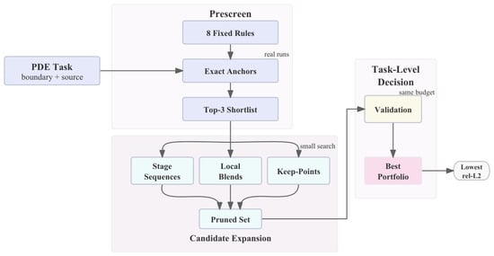
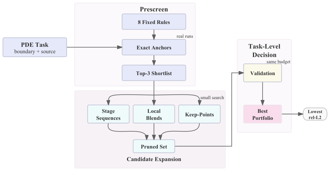
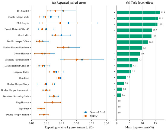
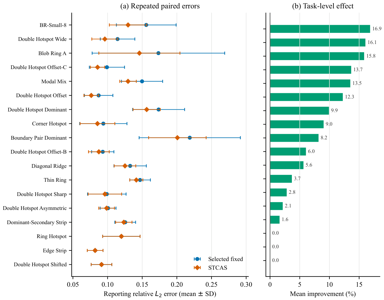
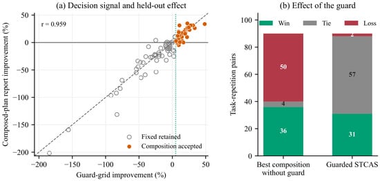
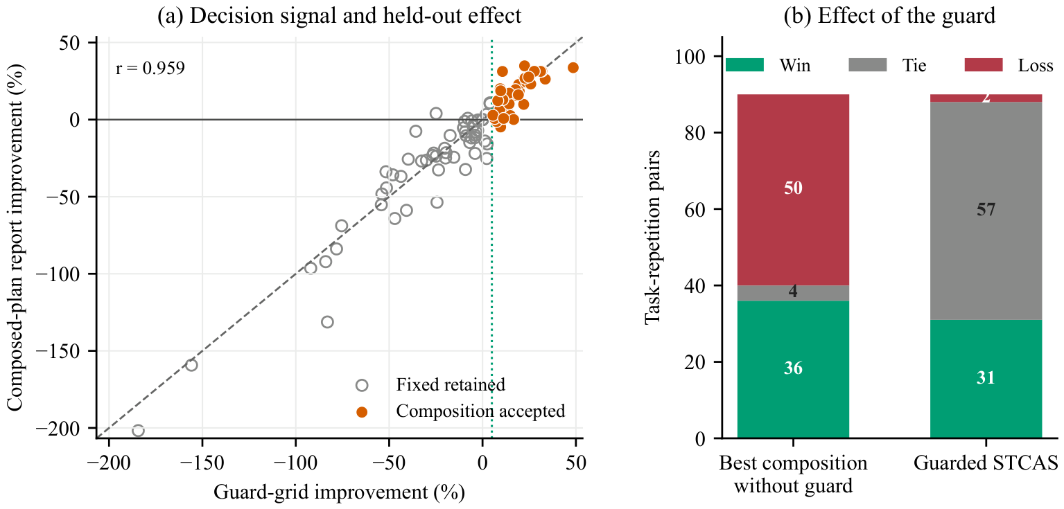
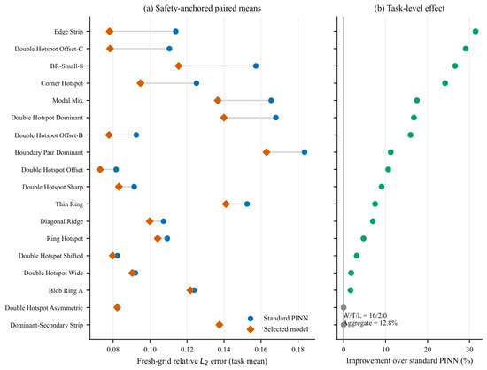
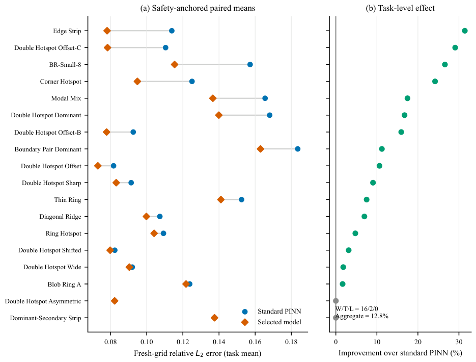
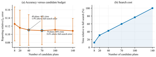
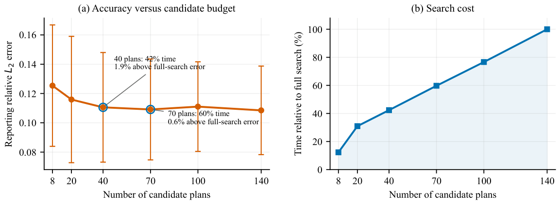
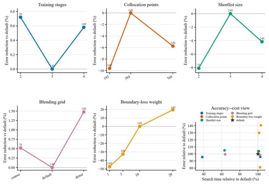
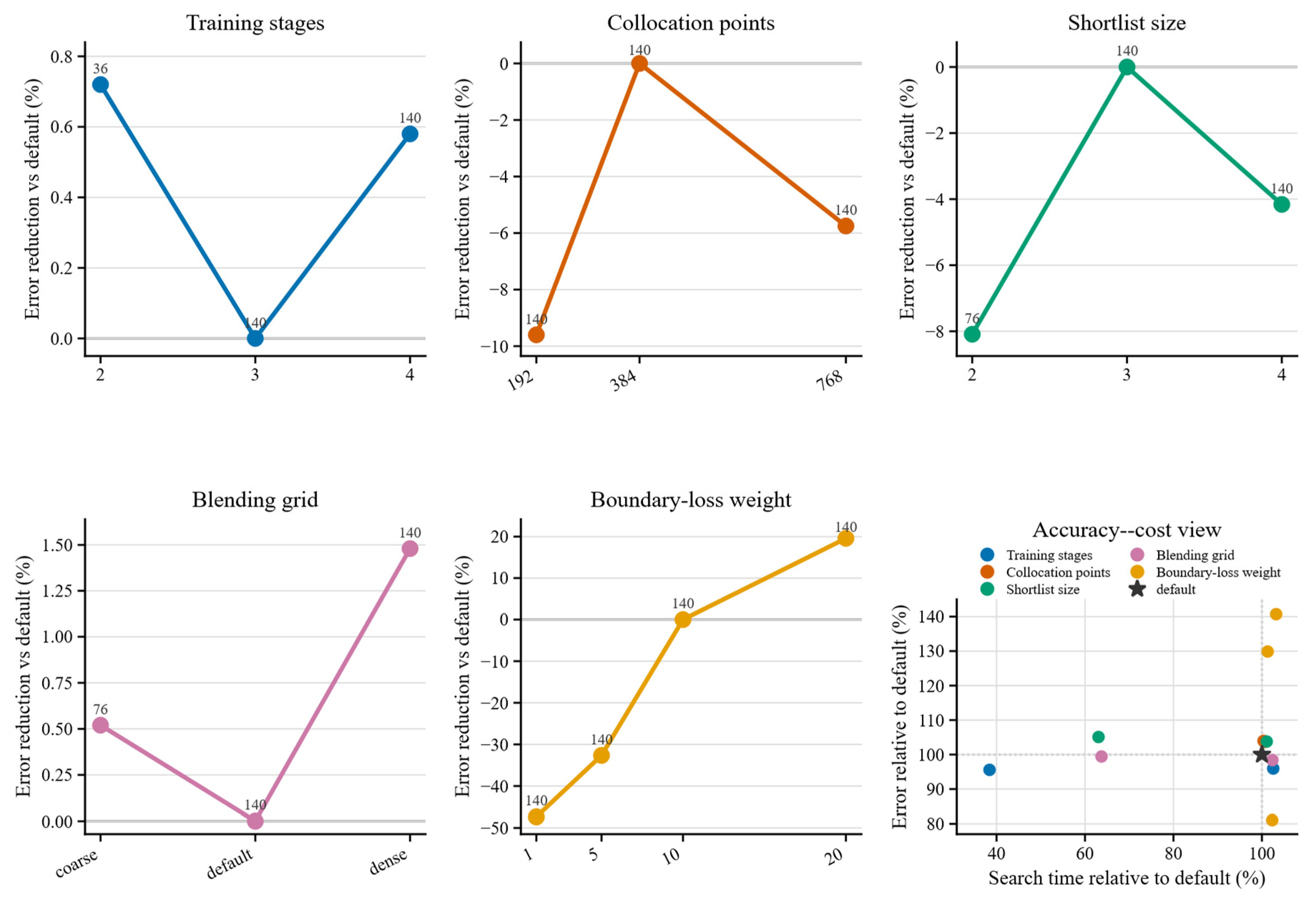

Disclaimer/Publisher’s Note: The statements, opinions and data contained in all publications are solely those of the individual author(s) and contributor(s) and not of MDPI and/or the editor(s). MDPI and/or the editor(s) disclaim responsibility for any injury to people or property resulting from any ideas, methods, instructions or products referred to in the content. |
© 2026 by the authors. Licensee MDPI, Basel, Switzerland. This article is an open access article distributed under the terms and conditions of the Creative Commons Attribution (CC BY) license.