Graph-X: Graph-Structured Deep Learning for Price Forecasting and Risk-Aware Virtual Power Plant Market Participation

Abstract

The increasing integration of distributed energy resources, renewable generation, and flexible loads has made Virtual Power Plant (VPP) market participation highly exposed to price volatility and operational uncertainty. This paper proposes Graph-X, a unified graph-structured deep learning and stochastic optimization framework for day-ahead electricity price forecasting and risk-aware VPP bidding. Unlike conventional temporal forecasting models, Graph-X captures structural market-clearing behavior by converting raw bids into continuous differentiable curves represented on a discrete price–quantity graph. The proposed architecture combines sparse graph convolutions, recurrent temporal learning, dilated temporal convolutions, and cyclical calendar encodings to model spatial, temporal, and operational market dependencies. Forecasts are further integrated with a stochastic bidding model governed by a coherent spectral risk measure to align prediction accuracy with financial performance. The framework is validated using historical hourly data from the ISO New England day-ahead electricity market. Results show that Graph-X achieves an MAE of 1.81 $/MWh and an R² score of 0.944, outperforming GNN, LSTM, Transformer, and ARIMA baselines. In VPP bidding, Graph-X delivers an average daily profit of 52.3 k$, improving profitability by 18.1% (equivalent to $2.92 annually) over the GNN baseline, with an average inference time of 12.5 ms per forecast.

1. Introduction

The rapid integration of renewable energy resources, distributed generation, battery storage, electric vehicles, and flexible demand has significantly changed modern electricity market operation [1]. Virtual Power Plants (VPPs) have emerged as an effective mechanism for aggregating heterogeneous distributed energy resources into a coordinated market participant [2]. Early VPP studies showed that distributed energy resources can be coordinated to support market participation and system-level flexibility [3]. Subsequent research extended the VPP concept toward optimized scheduling and coordinated energy management under operational constraints. VPPs can participate in electricity markets by offering aggregated generation, storage flexibility, and demand response services [4,5].

However, VPP market participation remains difficult because renewable generation is uncertain and intermittent [6]. Electricity price uncertainty further increases the financial risk of VPP bidding decisions. Load demand variability also affects the ability of a VPP to satisfy market commitments reliably [7,8]. Therefore, accurate electricity price forecasting is essential for improving VPP bidding and operational decision-making [9]. Classical electricity price forecasting studies have analyzed price spikes, seasonality, volatility, and market uncertainty [10]. Probabilistic forecasting methods have also been proposed to represent uncertainty in electricity price prediction. Recent research shows that machine learning can improve day-ahead electricity price forecasting compared with traditional statistical models [11,12]. Neural network-based forecasting models are effective because they can learn nonlinear relationships in electricity market data [13]. LSTM models have been widely used for electricity price forecasting due to their ability to capture long-term temporal dependencies [14]. GRU-based models provide a simpler recurrent structure while preserving temporal learning capability [15]. CNN-LSTM architectures have also been used to extract local temporal patterns and sequential dependencies jointly. Temporal convolutional networks are useful for price forecasting because they capture long-range dependencies using dilated causal convolutions [16,17].

Transformer-based models have improved multi-horizon forecasting by using attention mechanisms for temporal feature selection. Despite these advances, many deep learning methods treat electricity prices mainly as time-series signals [18,19]. Such models often ignore the explicit supply–demand structure and market-clearing behavior of electricity markets [20]. Graph neural networks provide a useful way to model structural relationships among nodes in complex systems [21]. Graph convolutional networks have been applied to learn localized structural patterns from graph-based data [22]. Graph attention networks further improve graph learning by assigning adaptive importance to neighboring nodes [23]. Recent electricity forecasting studies show that graph-based models can capture spatial dependence among market zones and price areas [24]. Spatio-temporal graph neural networks can jointly model temporal price evolution and structural relationships in electricity markets. Graph-based electricity price forecasting has therefore become an important direction for market-aware prediction [25,26].

However, most graph-based electricity forecasting studies focus mainly on prediction accuracy [27]. They rarely connect graph-based forecasting with VPP bidding decisions and market participation outcomes [28]. In parallel, VPP bidding strategies have been studied using stochastic programming under uncertain renewable generation and market prices. Robust optimization has also been used to support VPP bidding under uncertainty [29,30]. CVaR-based risk measures are useful for controlling downside financial risk in electricity market participation [31]. Risk-aware VPP bidding models improve decision-making by balancing expected profit and market uncertainty. Strategic bidding studies have considered VPP participation in day-ahead and real-time electricity markets [32]. Joint energy and reserve market participation has also been investigated for VPPs with flexible resources. Recent studies have considered multi-level energy interaction among VPP resources for day-ahead bidding [33]. Other works have examined renewable-based VPP offering and bidding strategies in electricity markets. Although these optimization-based methods are valuable, they often do not exploit graph-based deep learning for market-clearing representation. They also rarely learn nonlinear feature-lag relationships from electricity market data [34]. This creates a gap between forecasting accuracy, bidding optimization, and practical VPP market performance [35]. The proposed Graph-X framework addresses this gap by integrating VPP resource coordination, stochastic uncertainty modeling, graph-structured market representation, sparse graph convolution, temporal learning, and risk-aware bidding into a unified model.

The research gap is that existing studies generally address electricity price forecasting, graph-based market modeling, and VPP bidding optimization as separate problems and the comparison of literature are shown in Table 1. Forecasting models often ignore the explicit supply–demand and price–quantity structure of market clearing, while optimization-based VPP bidding models do not fully learn nonlinear market behavior from data. Moreover, graph-based forecasting studies usually report accuracy improvements without connecting them to VPP profit, bidding effectiveness, inference speed, and practical market participation.

Table 1. Comparative analysis of VPP market participation and price forecasting models.

Reference	Application	Forecasting Method	Graph Modeling	Learning Framework	Risk Handling	Optimization Strategy	Economic Evaluation
[1]	VPP coordination	–	–	Mathematical model	CVaR	Stochastic optimization	Profit analysis
[2]	Electricity price	Statistical forecasting	–	Statistical model	–	–	–
[3]	Price forecasting	Price prediction	–	Neural network	Risk assessment	–	–
[4]	VPP operation	Joint forecasting	–	Deep learning	Risk-aware scheduling	Bidding optimization	Economic analysis
[16]	Price forecasting	Price prediction	Market graph	GNN	–	–	–
[23]	VPP management	–	Graph learning	GNN	Risk-aware control	Bidding optimization	Profit analysis
[26]	Price forecasting	Price prediction	Graph representation	Deep learning	–	–	–
[35]	Market forecasting	Price prediction	Graph learning	Deep learning	–	–	–
Proposed Graph-X	VPP market participation	Day-ahead LMP forecasting	Price–quantity market graph	Sparse GCN + GRU + TCN	Spectral risk measure	Stochastic bidding	Profit and risk-adjusted return

This paper proposes Graph-X, a unified graph-based deep learning framework that integrates electricity price forecasting and VPP market bidding optimization within a single decision-making architecture. By coupling market-aware forecasting with stochastic bidding optimization, the proposed framework improves both prediction accuracy and economic performance.

The main contributions of this work are summarized as follows:

• A unified Graph-X framework is developed to jointly perform electricity price forecasting and risk-aware VPP bidding optimization through a graph-based market representation.
• A hybrid learning architecture combining sparse graph convolution, GRU, TCN, and calendar feature encoding is proposed to capture structural and temporal dependencies in electricity markets.
• A stochastic risk-aware bidding strategy is integrated with the forecasting model, directly linking prediction results to practical VPP market participation and profit optimization.
• Comprehensive validation against GNN, LSTM, Transformer, ARIMA, Graph Transformer, Temporal Fusion Transformer (TFT), and no-optimization baselines demonstrates superior forecasting accuracy, economic performance, and computational efficiency.

2. Mathematical Modeling

This section presents the mathematical formulation of the proposed Graph-X framework for Virtual Power Plant (VPP) market participation and day-ahead electricity price forecasting. The model integrates VPP resource coordination, uncertainty quantification, graph-based market representation, strategic bidding optimization, and deep learning within a unified framework. The formulation consists of three components: VPP operation and uncertainty modeling (Section 2.1), graph-based market representation and bidding optimization (Section 2.2), and Graph-X architecture with training strategy (Section 2.3).

2.1. Virtual Power Plant Resource Coordination and Uncertainty Quantification

The VPP aggregates heterogeneous distributed energy resources to enable coordinated market participation while managing diverse operational constraints and uncertainty sources. This section develops the mathematical framework for resource coordination and establishes the stochastic processes governing system uncertainties.

2.1.1. Aggregated Resource Coordination Framework

Consider a VPP-comprising dispatchable generation units indexed by $g\in \mathcal{G}=\{1,\dots ,G\}$, renewable energy sources indexed by $r\in \mathcal{R}=\{1,\dots ,R\}$, energy storage systems indexed by $s\in \mathcal{S}=\{1,\dots ,S\}$, and flexible demand resources indexed by $d\in \mathcal{D}=\{1,\dots ,D\}$. The operational horizon spans $T$ intervals of duration $\Delta t$, with $t\in \mathcal{T}=\{1,\dots ,T\}$. The net power injection of the VPP at interval $t$ incorporates contributions from all resource categories along with coupling effects and aggregation losses. This relationship is expressed in (1), where the commitment status of each resource is governed by binary variables and $\mathsf{\Lambda }(\cdot ,{\mathsf{\theta }}_{\mathrm{agg}})$ captures nonlinear aggregation effects including transmission losses and resource coupling interactions:

$$\begin{array}{c}{P}_{\mathrm{VPP}}\left(t\right)={\displaystyle {\displaystyle \sum }_{g\in \mathcal{G}}}{u}_g\left(t\right)P_g\left(t\right)+{\displaystyle {\displaystyle \sum }_{r\in \mathcal{R}}}{v}_r\left(t\right){\widehat{P}}_r\left(t\right)+{\displaystyle {\displaystyle \sum }_{s\in \mathcal{S}}}{w}_s\left(t\right)\\ \left(P_s^{\mathrm{dis}}\left(t\right)-P_s^{\mathrm{ch}}\left(t\right)\right)-{\displaystyle {\displaystyle \sum }_{d\in \mathcal{D}}}{z}_d\left(t\right)\Delta L_d\left(t\right)+\mathsf{\Lambda }\left(\mathrm{P}\left(t\right),{\mathsf{\theta }}_{\mathrm{agg}}\right)\end{array}$$

(1)

The aggregation loss function can be further decomposed into quadratic and linear forms, as shown in (2), where ${\mathsf{\Theta }}_{\mathrm{loss}}$ is a positive semi-definite matrix capturing pairwise resource interactions:

$$\mathsf{\Lambda }\left(\mathrm{P}\left(t\right),{\mathsf{\theta }}_{\mathrm{agg}}\right)=\mathrm{P}{(t)}^{\top }{\mathsf{\Theta }}_{\mathrm{loss}}\mathrm{P}\left(t\right)+{\mathsf{\theta }}_0^{\top }\mathrm{P}\left(t\right)$$

(2)

For compactness in subsequent derivations, the net storage contribution is defined in (3) as the difference between discharging and charging power:

$$P_s^{\mathrm{net}}\left(t\right)=P_s^{\mathrm{dis}}\left(t\right)-P_s^{\mathrm{ch}}\left(t\right)$$

(3)

The commitment states for dispatchable units must respect physical minimum up and down times. The constraint set (4) enforces that once a unit is started, it remains online for at least $T_g^{\mathrm{up}}$ consecutive intervals, while also ensuring minimum offline duration after shut-down:

$$\left\{\begin{array}{c}{\displaystyle {\displaystyle \sum }_{\tau =t-T_g^{\mathrm{up}}+1}^t}\max \left\{0,u_g\left(\tau \right)-u_g\left(\tau -1\right)\right\}\le u_g\left(t\right),\forall t\ge T_g^{\mathrm{up}}\\ {\displaystyle {\displaystyle \sum }_{\tau =t-T_g^{\mathrm{dn}}+1}^t}\max \left\{0,u_g\left(\tau -1\right)-u_g\left(\tau \right)\right\}\le 1-u_g\left(t\right),\forall t\ge T_g^{\mathrm{dn}}\\ u_g\left(t\right)-u_g\left(t-1\right)=y_g^{\mathrm{su}}\left(t\right)-y_g^{\mathrm{sd}}\left(t\right),y_g^{\mathrm{su}}\left(t\right)+y_g^{\mathrm{sd}}\left(t\right)\le 1\end{array}\right.$$

(4)

The binary variables $y_g^{\mathrm{su}}\left(t\right)$ and $y_g^{\mathrm{sd}}\left(t\right)$ in (4) represent start-up and shut-down commands respectively, with their mutual exclusivity preventing simultaneous contradictory signals. The power output of each dispatchable generator is bounded by its minimum stable level and maximum capacity when committed, as expressed in (5):

$$u_g\left(t\right)P_g^{\min }\le P_g\left(t\right)\le u_g\left(t\right)P_g^{\max }$$

(5)

Ramping constraints between consecutive intervals are captured in (6), where the big-M formulation relaxes constraints when units are offline. The parameters $R_g^{\mathrm{up}}$ and $R_g^{\mathrm{dn}}$ denote upward and downward ramp rates, respectively:

$$-R_g^{\mathrm{dn}}\Delta t-M\left(1-u_g\left(t\right)\right)\le P_g\left(t\right)-P_g\left(t-1\right)\le R_g^{\mathrm{up}}\Delta t+M\left(1-u_g\left(t-1\right)\right)$$

(6)

During start-up and shut-down transients, additional ramp limits apply due to thermal stresses. These are given in (7) and (8), where $S_g^{\mathrm{up}}$ and $S_g^{\mathrm{dn}}$ represent start-up and shut-down ramp capabilities:

$$P_g\left(t\right)\le P_g\left(t-1\right)+R_g^{\mathrm{up}}\Delta t\cdot u_g\left(t-1\right)+S_g^{\mathrm{up}}{y}_g^{\mathrm{su}}\left(t\right)+M\left(1-u_g\left(t\right)\right)$$

(7)

$$P_g\left(t-1\right)-P_g\left(t\right)\le R_g^{\mathrm{dn}}\Delta t\cdot u_g\left(t\right)+S_g^{\mathrm{dn}}{y}_g^{\mathrm{sd}}\left(t\right)+M\left(1-u_g\left(t-1\right)\right)$$

(8)

For energy storage systems, the state-of-charge evolution incorporates efficiency losses, self-discharge, and cycle-dependent degradation. The complete storage dynamics are captured in (9), where ${\epsilon }_s$ is the self-discharge rate, ${\eta }_s^{\mathrm{ch}}$ and ${\eta }_s^{\mathrm{dis}}$ are charging and discharging efficiencies, and ${\delta }_s(\cdot ,\cdot )$ represents temperature-dependent leakage:

$$\left\{\begin{array}{c}{E}_s\left(t\right)=E_s\left(t-1\right)\cdot \left(1-{\epsilon }_s\right)+\Delta t\left({\eta }_s^{\mathrm{ch}}{P}_s^{\mathrm{ch}}\left(t\right)-{\displaystyle \frac{P_s^{\mathrm{dis}}\left(t\right)}{{\eta }_s^{\mathrm{dis}}}}\right)-{\delta }_s\left(E_s\left(t-1\right),T_s^{\mathrm{amb}}\right)\\ E_s^{\min }\le E_s\left(t\right)\le E_s^{\max }-{\rho }_s\cdot N_s^{\mathrm{cyc}}\left(t\right)\\ 0\le P_s^{\mathrm{ch}}\left(t\right)\le P_s^{\mathrm{ch},\max }\cdot b_s\left(t\right),b_s\left(t\right)\in \left\{0,1\right\}\\ 0\le P_s^{\mathrm{dis}}\left(t\right)\le P_s^{\mathrm{dis},\max }\cdot \left(1-b_s\left(t\right)\right)\end{array}\right.$$

(9)

The temperature-dependent leakage term in (9) is linearized around the nominal operating temperature in (10), where ${\beta }_s$ is the temperature coefficient:

$${\delta }_s\left(E,T\right)={\delta }_s^0\cdot E\cdot \left(1+{\beta }_s\left(T-T_{\mathrm{nom}}\right)\right)$$

(10)

Cycle counting for degradation tracking follows the symmetric depth-of-discharge metric in (11), where each half-cycle of significant depth contributes to cumulative wear:

$$N_s^{\mathrm{cyc}}\left(t\right)=N_s^{\mathrm{cyc}}\left(t-1\right)+{\displaystyle \frac{1}{2}}\left|b_s\left(t\right)-b_s\left(t-1\right)\right|\cdot {\displaystyle \frac{\left|E_s\left(t\right)-E_s\left(t-1\right)\right|}{E_s^{\max }}}$$

(11)

The charging/discharging mutual exclusivity can be relaxed for certain storage technologies, leading to the complementary slackness condition expressed in (12):

$$P_s^{\mathrm{ch}}\left(t\right)\cdot P_s^{\mathrm{dis}}\left(t\right)=0$$

(12)

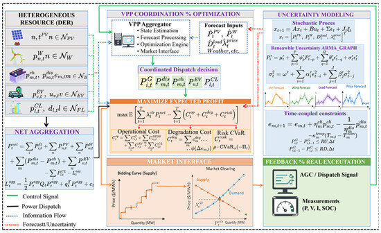
As illustrated in Figure 1, the VPP aggregates heterogeneous energy resources through coordinated information flows while accounting for temporal constraints and uncertainties in renewable generation, load demand, and market prices. Flexible demand resources provide load adjustment subject to consumer comfort and recovery constraints. The constraint set (13) imposes limits on reduction magnitude, cumulative reduction budgets, minimum service levels, and event frequency within rolling windows. The recovery period ${\tau }_d^{\mathrm{rec}}$ in (13) ensures load restoration within acceptable timeframes, preventing prolonged demand suppression that could violate consumer comfort.

$$\left\{\begin{array}{c}0\le \Delta L_d\left(t\right)\le \Delta L_d^{\max }\cdot z_d\left(t\right)\\ {\displaystyle {\displaystyle \sum }_{\tau =t-{\tau }_d^{\mathrm{rec}}}^t}\Delta L_d\left(\tau \right)\le \Delta L_d^{\mathrm{total}}\\ L_d^{\mathrm{base}}\left(t\right)-\Delta L_d\left(t\right)\ge L_d^{\min }\\ {\displaystyle {\displaystyle \sum }_{\tau =t_0}^{t_0+T_d^{\mathrm{win}}}}{z}_d\left(\tau \right)\le N_d^{\max },\forall t_0\in \left\{1,\dots ,T-T_d^{\mathrm{win}}\right\}\end{array}\right.$$

(13)

Figure 1. Virtual Power Plant resource aggregation architecture with information flows, temporal constraints, and uncertainty propagation from renewable, load, and price nodes.

2.1.2. Stochastic Uncertainty Quantification

The constraints formulated in (1)–(13) operate under imperfect information. Renewable generation ${\widehat{P}}_r\left(t\right)$ is inherently stochastic, market-clearing prices are unknown at bidding time, and actual demand deviates from forecasts. We therefore construct a multivariate stochastic process that captures the joint evolution of these uncertainties.

Define the complete uncertainty vector $\mathsf{\xi }\left(t\right)=\left[{\mathsf{\xi }}^R\right(t{)}^{\top },{\xi }^P\left(t\right),{\mathsf{\xi }}^D(t{)}^{\top }{]}^{\top }\in {\mathbb{R}}^{R+1+D}$. Its dynamics follow the coupled system in (14), combining autoregressive behavior, Gaussian innovations, and Poisson-driven jumps. The state transition matrix $\mathsf{\Phi }\left(t\right)$ captures temporal correlations across components:

$$\left\{\begin{array}{c}\xi \left(t\right)=\Phi \left(t\right)\xi \left(t-1\right)+\mathsf{\Theta }\left(t\right)\epsilon \left(t\right)+J\left(t\right)\circ N\left(t;\lambda \right)\\ \epsilon \left(t\right)\sim N\left(0,{\mathsf{\Sigma }}_{\epsilon }\left(t\right)\right),{\mathsf{\Sigma }}_{\epsilon }\left(t\right)=L\left(t\right)L{(t)}^{\top }+D\left(t\right)\\ N\left(t;\lambda \right)={[N_1\left(t;{\lambda }_1\right),\dots ,N_{R+1+D}\left(t;{\lambda }_{R+1+D}\right)]}^{\top }\\ N_k\left(t;{\lambda }_k\right)\sim \mathrm{Poisson}\left({\lambda }_k\Delta t\right),\forall k\in \left\{1,\dots ,R+1+D\right\}\end{array}\right.$$

(14)

The jump term in (14) incorporates random magnitudes through $\mathrm{J}\left(t\right)=\mathsf{{\rm Y}}\left(t\right)\odot \mathrm{Z}\left(t\right)$ with $\mathrm{Z}\left(t\right)\sim \mathcal{N}({\mathsf{\mu }}_J,{\mathsf{\Sigma }}_J)$. The covariance decomposition ${\mathsf{\Sigma }}_{\epsilon }\left(t\right)=\mathrm{L}\left(t\right)\mathrm{L}(t{)}^{\top }+\mathrm{D}(t)$ enables efficient representation of both common shocks and idiosyncratic variations, where $\mathrm{L}\left(t\right)$ is a low-rank factor matrix and $\mathrm{D}\left(t\right)$ is diagonal.

For renewable generation specifically, the uncertainty structure must respect physical constraints. The physics-informed parameterization in (15) relates actual generation to its forecast through a time-varying coefficient of variation $c_v^r\left(t\right)$:

$${\xi }_r^R\left(t\right)={\displaystyle \frac{{\widehat{P}}_r\left(t\right)-{\stackrel{-}{P}}_r\left(t\right)}{{\sigma }_r^P\left(t\right)}},{\widehat{P}}_r\left(t\right)=P_r^{\mathrm{rated}}\cdot f_r\left({\mathrm{W}}_r\left(t\right);{\varphi }_r\right)\cdot \left(1+{\xi }_r^R\left(t\right)\cdot c_v^r\left(t\right)\right)$$

(15)

The power curve $f_r(\cdot )$ in (15) maps meteorological variables ${\mathrm{W}}_r\left(t\right)$ to generation, combining a kernel integral for nonlinear conversion characteristics with a site-specific correction term. This relationship is expanded in (16):

$$f_r\left({\mathrm{W}}_r\left(t\right);{\varphi }_r\right)={{\displaystyle \int }}_{w_{\min }}^{w_{\max }}{\kappa }_r\left(w;{\varphi }_r\right)\cdot g_r\left(w,{\mathrm{W}}_r\left(t\right)\right)dw+h_r\left({\mathrm{W}}_r\left(t\right);{\mathsf{\psi }}_r\right)$$

(16)

Meteorological variables themselves evolve according to the vector autoregressive process of order one in (17), where ${\mathrm{A}}_r$ and ${\mathrm{B}}_r$ are coefficient matrices and ${\mathsf{\eta }}_r\left(t\right)$ is Gaussian white noise:

$${\mathrm{W}}_r\left(t\right)={\mathrm{A}}_r{\mathrm{W}}_r\left(t-1\right)+{\mathrm{B}}_r{\mathsf{\eta }}_r\left(t\right),{\mathsf{\eta }}_r\left(t\right)\sim \mathcal{N}\left(0,{\mathrm{Q}}_r\right)$$

(17)

Electricity price uncertainty exhibits distinct stylized facts: mean reversion, volatility clustering, and sensitivity to renewable infeed. The regime-switching process in (18) captures these features, where the regime variable $m\left(t\right)\in \{1,\dots ,M\}$ follows a Markov chain:

$$\left\{\begin{array}{c}{\xi }^P\left(t\right)=log\left({\displaystyle \frac{\pi \left(t\right)}{\pi \left(t-1\right)}}\right)-{\mu }_{\pi }\left(t,m\left(t\right)\right)\\ {\mu }_{\pi }\left(t,m\right)={\alpha }_m\left({\beta }_m-log\pi \left(t-1\right)\right)\Delta t+{\gamma }_m\cdot \left({\displaystyle \frac{1}{R}}{\displaystyle {\displaystyle \sum }_{r=1}^R}{\xi }_r^R\left(t\right)\right)\Delta t\\ {\sigma }_{\pi }^2\left(t,m\right)={\omega }_m+{\varphi }_m{\sigma }_{\pi }^2\left(t-1,m\right)+{\psi }_m{({\xi }^P\left(t-1\right))}^2\\ P\left(m\left(t\right)=j\mid m\left(t-1\right)=i\right)=p_{ij},{\displaystyle {\displaystyle \sum }_{j=1}^M}{p}_{ij}=1,\forall i\end{array}\right.$$

(18)

The mean-reversion speed ${\alpha }_m$ and long-term mean ${\beta }_m$ in (18) are regime-dependent, as is the sensitivity ${\gamma }_m$ to aggregate renewable generation. The volatility follows GARCH (1,1) dynamics with regime-specific parameters ${\omega }_m,{\varphi }_m,{\psi }_m$.

The log-price return can be related to the original price through the inverse transformation in (19), which is useful for scenario generation:

$$\pi \left(t\right)=\pi \left(t-1\right)\cdot \exp \left({\mu }_{\pi }\left(t,m\left(t\right)\right)+{\xi }^P\left(t\right)\right)$$

(19)

Demand uncertainty decomposes into systematic patterns and residual variation. The base load model in (20) combines Fourier harmonics for diurnal periodicity with indicator functions for special periods ${\mathcal{H}}_p$:

$$L_d^{\mathrm{base}}\left(t\right)={\mu }_d^0+{\displaystyle {\displaystyle \sum }_{h=1}^{H_d}}{\nu }_{d,h}\sin \left({\displaystyle \frac{2\pi ht}{24}}\right)+{\displaystyle {\displaystyle \sum }_{h=1}^{H_d}}{\omega }_{d,h}\cos \left({\displaystyle \frac{2\pi ht}{24}}\right)+{\displaystyle {\displaystyle \sum }_{p=1}^{P_d}}{\zeta }_{d,p}{1}_{\left\{t\in {\mathcal{H}}_p\right\}}$$

(20)

Exogenous variables such as temperature and humidity contribute linearly to demand, as shown in (21) with coefficients ${\theta }_{d,k}$:

$$L_d^{\mathrm{exog}}\left(t\right)={\displaystyle {\displaystyle \sum }_{k=1}^K}{\theta }_{d,k}{X}_{d,k}\left(t\right)$$

(21)

The volatility function in (22) follows an exponential parameterization that scales with peak periods through factor ${\tau }_d$

$${\sigma }_d^L\left(t\right)=\exp \left({\eta }_d^0+{\displaystyle {\displaystyle \sum }_{q=1}^{Q_d}}{\eta }_{d,q}{1}_{\left\{t\in {\mathcal{S}}_q\right\}}\right)\cdot \left(1+{\tau }_d\cdot 1_{\left\{t\in {\mathcal{T}}_{\mathrm{peak}}\right\}}\right)$$

(22)

The normalized demand uncertainty is then expressed in (23) as the ratio of residual to its time-varying standard deviation:

$${\xi }_d^D\left(t\right)={\displaystyle \frac{L_d^{\mathrm{actual}}\left(t\right)-L_d^{\mathrm{base}}\left(t\right)-L_d^{\mathrm{exog}}\left(t\right)}{{\sigma }_d^L\left(t\right)}}$$

(23)

While marginal distributions are essential, the joint dependence among uncertainty components critically determines portfolio risk. The copula-based dependence structure in (24) captures both upper and lower tail dependencies. The Gumbel–Hougaard copula with parameter ${\nu }_1$ handles extreme co-movements, while pair-copula terms $c_{ij}(\cdot ,\cdot )$ accommodate heterogeneous bivariate dependencies:

$$\left\{\begin{array}{c}{\mathrm{C}}_{\mathsf{\xi }}\left(u;\nu \right)=exp\left(-{\left[{\displaystyle {\displaystyle \sum }_{k=1}^{R+1+D}}{(-\log u_k)}^{{\nu }_1}\right]}^{1/{\nu }_1}\right)\cdot {\displaystyle {\displaystyle \prod }_{i<j}}{c}_{ij}\left(u_i,u_j;{\nu }_{ij}\right)\\ {\tau }_{ij}^K=4{{\displaystyle \int }}_0^1{{\displaystyle \int }}_0^1{\mathrm{C}}_{ij}\left(u_i,u_j;{\nu }_{ij}\right)\hspace{0.17em}d{\mathrm{C}}_{ij}\left(u_i,u_j;{\nu }_{ij}\right)-1\\ {\lambda }_{ij}^U=\underset{u\to 1^{-}}{\lim }{\displaystyle \frac{1-2u+{\mathrm{C}}_{ij}\left(u,u;{\nu }_{ij}\right)}{1-u}},{\lambda }_{ij}^L=\underset{u\to 0^{+}}{\lim }{\displaystyle \frac{{\mathrm{C}}_{ij}\left(u,u;{\nu }_{ij}\right)}{u}}\end{array}\right.$$

(24)

The measures ${\tau }_{ij}^K$, ${\lambda }_{ij}^U$, and ${\lambda }_{ij}^L$ in (24) quantify Kendall’s rank correlation, upper tail dependence, and lower tail dependence respectively. These are critical for risk-aware decision-making under extreme market conditions.

2.2. Graph-Theoretic Market Representation and Stochastic Bidding Optimization

The market-clearing mechanism determines the equilibrium price and dispatched quantities through the intersection of aggregated supply and demand curves. To capture both the structural characteristics of market bids and their economic interactions, the electricity market is represented as a graph. Unlike conventional time-series models, the proposed market graph preserves price–quantity relationships and supply–demand interactions, where each node represents a price–quantity state and the edges describe spatial and economic relationships. This graph-based representation enables effective extraction of market-aware features for electricity price forecasting and VPP bidding optimization. The market bidding graph is defined as.

Define the market bidding graph as:

$$G_M=\left(V_M,E_M,X_M,A_M\right)$$

(25)

where (V_M) denotes the set of graph vertices, (E_M) represents the edge set, (X_M) denotes node features, and (A_M) is the weighted adjacency matrix. The vertices correspond to discretized price–quantity coordinates forming a two-dimensional grid with resolution $(∆ p\times ∆q)$. Therefore, the total number of graph nodes is:

$$\mid V_M\mid =H\times W$$

(26)

where

$$H={\displaystyle \frac{p_{max}-p_{min}}{\Delta p}},$$

(27)

$$W={\displaystyle \frac{q_{max}-q_{min}}{\Delta q}}.$$

(28)

Before graph construction, the submitted discrete market bids are transformed into continuous differentiable supply and demand curves. For a supply-side participant (i) submitting (J_i) price–quantity pairs, the aggregated supply curve at price (p) is expressed as:

$$\{\begin{array}{c}{Q}_S\left(p,t\right)={{\displaystyle \sum }}_{i\in I_S}{{\displaystyle \sum }}_{j=1}^{J_i}{q}_{i,j}\left(t\right)1_{\left\{p\ge p_{i,j}\left(t\right)\right\}}{1}_{\left\{{\alpha }_i\left(t\right)=1\right\}}+{{\displaystyle \int }}_{p_{min}}^p{\varphi }_S\left(\xi ,t\right)d\xi \\ {\varphi }_S\left(p,t\right)={{\displaystyle \sum }}_{k=1}^{K_S}{\beta }_k^S\left(t\right){\psi }_k\left(p;{\theta }_k^S\right)+{ϵ}_S\left(p,t\right)\end{array}$$

(29)

The basis functions (${\psi }_k(\cdot )$) combine sigmoid activation and Gaussian localization:

$${\psi }_k\left(p;{\theta }_k^S\right)={\displaystyle \frac{1}{1+\exp \left(-{\theta }_{k,1}^S\left(p-{\theta }_{k,2}^S\right)\right)}}\exp \left(-{\displaystyle \frac{{(p-{\theta }_{k,3}^S)}^2}{2{({\theta }_{k,4}^S)}^2}}\right)$$

(30)

which provides a differentiable approximation while maintaining the characteristics of stepwise market bids. Similarly, the aggregated demand curve is represented as:

$$\{\begin{array}{c}{Q}_D\left(p,t\right)={{\displaystyle \sum }}_{j\in I_D}{d}_{j,k}\left(t\right)1_{\left\{p\le p_{j,k}\left(t\right)\right\}}{1}_{\left\{{\beta }_j\left(t\right)=1\right\}}{{\displaystyle \sum }}_{k=1}^{K_j}+{{\displaystyle \int }}_p^{p_{max}}{\varphi }_D\left(\xi ,t\right)d\xi \\ {\varphi }_D\left(p,t\right)={{\displaystyle \sum }}_{l=1}^{K_D}{\gamma }_l^D\left(t\right){\varphi }_l\left(p;{\vartheta }_l^D\right)+{ϵ}_D\left(p,t\right)\end{array}$$

(31)

where the demand basis function is defined as:

$${\varphi }_l\left(p;{\vartheta }_l^D\right)=\tan \mathrm{h}\left({\vartheta }_{l,1}^D\left(p-{\vartheta }_{l,2}^D\right)\right)\exp \left(-{\vartheta }_{l,3}^D\mid p-{\vartheta }_{l,4}^D\mid \right)$$

(32)

Real market bids are discrete price–quantity pairs. We adopt a continuous approximation using smooth basis functions to enable differentiable graph-based learning. This does not model discrete clearing mechanisms (e.g., uniform pricing) exactly. Grid resolution controls approximation fidelity vs. computational cost.

The market-clearing price (p^*(t)) is obtained when the aggregated supply equals the aggregated demand:

$$Q_S\left(p^{*}\left(t\right),t\right)=Q_D\left(p^{*}\left(t\right),t\right)$$

(33)

This equilibrium point corresponds to the intersection of supply and demand surfaces embedded within the discretized price–quantity graph.

For each grid node ((h,w)), the node feature matrix (X_M) contains two channels representing supply and demand characteristics. The first channel describes supply-side information weighted by supply elasticity, whereas the second channel represents demand-side characteristics:

$$\{\begin{array}{c}{X}_M\left(h,w,1\right)=1_{\left\{Q_S\left(p_h,t\right)\ge q_w\right\}}{\displaystyle \frac{\partial Q_S\left(p,t\right)}{\partial p}}{\mid }_{p=p_h}{\delta }_S\left(h,w\right)\\ X_M\left(h,w,2\right)=1_{\left\{Q_D\left(p_h,t\right)\le q_w\right\}}\mid {\displaystyle \frac{\partial Q_D\left(p,t\right)}{\partial p}}{\mid }_{p=p_h}{\delta }_D\left(h,w\right)\end{array}$$

(34)

The modulation factors describing sub-grid positioning are:

$${\delta }_S\left(h,w\right)={\displaystyle \frac{p_{h}mod\Delta p}{\Delta p}}{\displaystyle \frac{q_{w}mod\Delta q}{\Delta q}}$$

(35)

$$p_h=p_{min}+h\Delta p,q_w=q_{min}+w\Delta q$$

(36)

The price and quantity coordinates of each graph node are obtained through affine mapping:

To represent the complex relationships existing among market states, the adjacency matrix (A_M) is constructed using three complementary edge mechanisms:

1.

Spatial adjacency edges:

These edges connect neighboring price–quantity nodes in the discretized grid and preserve local continuity of the market surface.

2.

Economic similarity edges:

These weighted edges connect economically similar nodes within a predefined (K)-neighborhood. The connection strength decreases according to the distance in price and quantity space using a Gaussian kernel.

3.

Supply–demand coupling edges:

These edges directly connect supply and demand nodes with equivalent dispatched quantities, representing the physical market-clearing interaction.

Accordingly, the weighted adjacency matrix is defined as:

$$A_M\left(\left(h,w\right),\left(h^{\prime },w^{\prime }\right)\right)=\{\begin{array}{cc}1,& \mid \mid \left(h,w\right)-\left(h^{\prime },w^{\prime }\right)\mid {\mid }_1=1\\ \exp \left(-{\displaystyle \frac{\mid p_h-p_{h^{\prime }}{\mid }^2}{2{\sigma }_p^2}}-{\displaystyle \frac{\mid q_w-q_{w^{\prime }}{\mid }^2}{2{\sigma }_q^2}}\right),& \left(h,w\right)\in N_K\left(h^{\prime },w^{\prime }\right)\\ 1,& Q_S\left(p_h,t\right)=q_w\wedge Q_D\left(p_{h^{\prime }},t\right)=q_{w^{\prime }}\\ 0,& otherwise\end{array}$$

(37)

where ($N_K(h,w)$) defines the (K)-neighborhood:

$$N_K\left(h,w\right)=\left\{\left(h^{\prime },w^{\prime }\right):\mid h-h^{\prime }\mid \le K,\mid w-w^{\prime }\mid \le K,\left(h,w\right)\ne \left(h^{\prime },w^{\prime }\right)\right\}$$

(38)

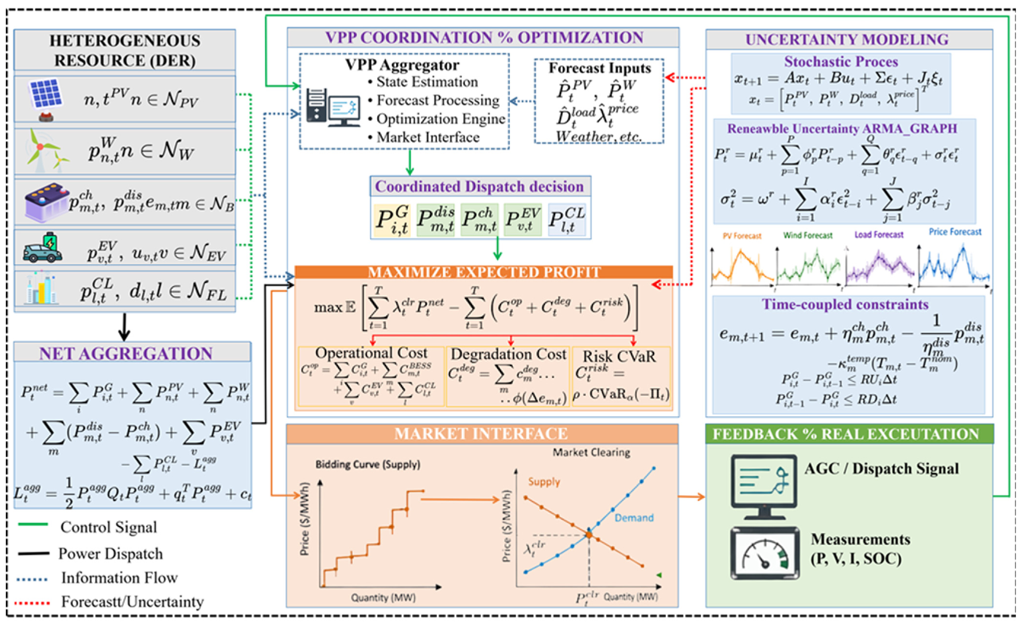
The first condition captures local spatial connectivity, the second assigns stronger weights to economically similar price–quantity states through Gaussian distance decay, and the third establishes direct market-clearing relationships between supply and demand nodes. Therefore, (A_M) integrates both geometric and economic information, enabling the sparse graph convolution module to learn meaningful market-clearing patterns. As illustrated in Figure 2, the aggregated supply and demand bids are transformed into a multi-edge market graph, enabling equilibrium price localization through discrete price–quantity grid encoding and graph-based market clearing.

Figure 2. Market-clearing graph construction from aggregated bid curves, discrete price–quantity grid encoding, multi-edge graph topology, and equilibrium price localization.

2.2.1. Stochastic Bidding Optimization Framework

The VPP participates in the electricity market by submitting price–quantity bids that reflect its aggregated resource capability, operational constraints, and risk preference. Since the actual market outcome depends on uncertain renewable generation, electricity prices, load variations, and competing participants’ bidding behaviors, the bidding strategy is formulated as a stochastic optimization problem. The objective is to maximize the expected economic return while controlling potential financial losses caused by unfavorable market realizations. Let the bidding decision of the VPP be represented by a supply offer curve consisting of $K_{VPP}$ price–quantity pairs:

$$B_{VPP}\left(t\right)={\left\{\left(p_k^{bid}\left(t\right),q_k^{bid}\left(t\right)\right)\right\}}_{k=1}^{K_{VPP}}$$

(39)

where ($p_k^{bid}\left(t\right)$) and ($q_k^{bid}\left(t\right)$) denote the submitted bidding price and quantity, respectively. Considering the uncertainty vector ($\xi$) characterized, the risk-aware stochastic bidding problem is formulated as:

$$\{\begin{array}{c}{\max }_{B_{VPP}\left(t\right)}{E}_{\xi }\left[{{\displaystyle \sum }}_{t=1}^T\pi \left(t\right)P_{cleared}\left(t\right)-C_{VPP}\left(P\left(t\right),\xi \left(t\right)\right)\right]-\lambda R\left(\mathsf{\Pi }\right)\\ s.t.P_{cleared}\left(t\right)={{\displaystyle \sum }}_{k=1}^{K_{VPP}}{q}_k^{bid}\left(t\right)1_{\left\{\pi \left(t\right)\ge p_k^{bid}\left(t\right)\right\}}\\ 0\le P_{cleared}\left(t\right)\le P_{VPP}^{max}\left(t\right)\\ p_k^{bid}\left(t\right)\le p_{k+1}^{bid}\left(t\right),q_k^{bid}\left(t\right)\ge 0,\forall k\\ Constraints\left(4\right)-\left(13\right)\end{array}$$

(40)

The probabilistic forecasts ${\widehat{Q}}_{\alpha }\left(t\right)$ generated by Graph-X serve as uncertainty inputs to this stochastic optimization problem. Specifically, the forecasted price distribution is used to sample market price scenarios $\pi \left(t\right)$ in the objective function, enabling the VPP to optimize bids under price uncertainty. This integration ensures that forecasting accuracy directly influences bidding decisions and economic outcomes.

The first term represents the expected market profit, while ($R\left(\Pi \right)$) represents the downside financial risk associated with uncertain market outcomes. The coefficient ($\lambda$) controls the tradeoff between economic performance and risk mitigation. A larger ($\lambda$) produces a more conservative bidding strategy by assigning greater importance to potential losses.

The cleared quantity is determined by comparing the realized market price with submitted bid prices. The monotonicity condition $p_k^{bid}\left(t\right)\le p_{k+1}^{bid}\left(t\right)$ ensures that the submitted supply curve remains physically meaningful and non-decreasing. The total VPP operating cost consists of generation operation cost, energy storage degradation cost, renewable curtailment penalty, and demand response compensation:

$$\{\begin{array}{c}{C}_{VPP}\left(P\left(t\right),\xi \left(t\right)\right)={{\displaystyle \sum }}_{g\in G}{C}_g\left(P_g\left(t\right)\right)+{{\displaystyle \sum }}_{s\in S}{C}_s^{deg}\left(P_s^{ch}\left(t\right),P_s^{dis}\left(t\right),E_s\left(t\right)\right)\\ +{{\displaystyle \sum }}_{r\in R}{C}_r^{curt}\left({\widehat{P}}_r\left(t\right)-P_r^{used}\left(t\right)\right)+{{\displaystyle \sum }}_{d\in D}{C}_d^{DR}\left(\Delta L_d\left(t\right)\right)\end{array}$$

(41)

The generation cost function considers conventional operating costs and nonlinear penalties associated with operation beyond technical limits:

$$C_g\left(P_g\right)=a_g{P}_g^2+b_g{P}_g+c_g+d_{g}exp\left(e_g{P}_g\right)+f_{g}max{\{0,P_g-P_g^{thr}\}}^3$$

(42)

The degradation cost of storage resources considers accumulated energy throughput, state-of-charge conditions, and temperature effects:

$$C_s^{deg}\left(\cdot \right)={\kappa }_s^0+{\kappa }_s^1\mid {\displaystyle \frac{P_s^{ch}\left(t\right)+P_s^{dis}\left(t\right)}{P_s^{max}}}{\mid }^{{\rho }_s}{\left({\displaystyle \frac{E_s\left(t\right)}{E_s^{max}}}\right)}^{-{\zeta }_s}\left(1+{\tau }_s\Delta T_s\left(t\right)\right)$$

(43)

To quantify financial uncertainty, a coherent spectral risk measure is adopted instead of relying only on expected profit or conventional variance-based risk metrics. The spectral formulation provides flexibility in assigning different importance levels to losses across the distribution and generalizes Conditional Value-at-Risk (CVaR). The risk measure is defined as:

$$\{\begin{array}{c}R\left(\mathsf{\Pi }\right)={{\displaystyle \int }}_0^1\varphi \left(u\right)Va{R}_u\left(-\mathsf{\Pi }\right)du\\ \varphi \left(u\right)={\displaystyle \frac{1}{\alpha }}{1}_{\left\{u\le \alpha \right\}}+{\displaystyle \frac{\beta }{\alpha \left(1-\beta \right)}}{1}_{\{u>\alpha \}}{u}^{-1/\gamma }\\ CVa{R}_{\alpha }\left(-\mathsf{\Pi }\right)={\displaystyle \frac{1}{\alpha }}{{\displaystyle \int }}_0^{\alpha }Va{R}_u\left(-\mathsf{\Pi }\right)du\end{array}$$

(44)

where ($\Pi$) represents the bidding profit distribution. The parameter ($\alpha$) defines the confidence level of extreme losses and is set to 0.05 in this study, corresponding to a 5% tail-risk region. The parameter ($\beta$) determines the emphasis assigned to severe losses beyond the VaR threshold, where larger values increase risk aversion by placing greater weight on unfavorable outcomes.

The parameter ($\gamma$) controls the decay behavior of the weighting function and regulates the transition between normal market fluctuations and extreme loss events. In this study, the values of ($\beta$) and ($\gamma$) are selected to achieve a balanced risk-return tradeoff. Specifically, excessively small ($\beta$) values may underestimate extreme market risks and lead to aggressive bidding decisions, while excessively large values may reduce profitability due to overly conservative operation. Similarly, ($\gamma$) is selected to provide smooth risk weighting without excessively penalizing moderate deviations. Therefore, the adopted spectral risk parameters provide an appropriate balance between expected profit maximization and protection against severe market uncertainty.

Market clearing with strategic VPP participation is formulated through an equilibrium condition, where the clearing price is determined by the interaction between the aggregated supply and demand curves. Unlike a pure price-taking formulation, the proposed model considers the influence of VPP bidding decisions through the aggregated supply function. The equilibrium price is obtained by minimizing the mismatch between total supply and demand:

$${\pi }^{\ast }\left(t\right)\in \arg \underset{\pi \ge 0}{\min }\mid Q_S^{agg}\left(\mathsf{\pi },\mathrm{t};{\theta }_S\right)-Q_D^{agg}\left(\mathsf{\pi },\mathrm{t};{\theta }_D\right)\mid$$

(45)

where (${\pi }^{*}\left(t\right)$) represents the market-clearing equilibrium price. The aggregated supply and demand functions include the contribution of the VPP and other market participants, which are expressed as:

$$\{\begin{array}{c}{Q}_S^{agg}\left(\pi ,t;{\theta }_S\right)=Q_S^{VPP}\left(\pi ,t\right)+{{\displaystyle \sum }}_{i\in I_S\setminus \left\{VPP\right\}}{Q}_{S,i}\left(\pi ,t;{\theta }_{S,i}\right)\\ Q_D^{agg}\left(\pi ,t;{\theta }_D\right)=Q_D^{VPP}\left(\pi ,t\right)+{{\displaystyle \sum }}_{j\in I_D\setminus \left\{VPP\right\}}{Q}_{D,j}\left(\pi ,t;{\theta }_{D,j}\right)\end{array}$$

(46)

The variational inequality in (41) ensures that the market equilibrium satisfies the physical and economic constraints while maintaining bidding feasibility.

Where ($Q_S^{VPP}\left(\pi ,t\right)$) and ($Q_D^{VPP}\left(\pi ,t\right)$) represent the VPP’s submitted supply and demand behaviors, respectively. Therefore, the VPP bidding strategy directly modifies the aggregated market curves and influences the resulting equilibrium price.

The market equilibrium is further characterized using a variational inequality formulation:

$$F\left(x^{*}\right),x-x^{*}\ge 0,\forall x\in K$$

(47)

where ($x^{*}$) denotes the equilibrium solution and (K) represents the feasible decision space incorporating market price limits, quantity constraints, operational constraints, and market power mitigation requirements. This equilibrium formulation enables the proposed framework to capture the interaction between VPP bidding decisions and market-clearing outcomes.

Although actual electricity markets employ discrete block bids and stepwise clearing prices, this study adopts a continuous approximation of the price–quantity relationship to construct the market graph and enable efficient learning of supply–demand interactions. The discretized graph representation preserves the essential economic characteristics of market clearing while avoiding excessive complexity caused by directly modeling all discrete bidding combinations. This assumption mainly affects the mathematical representation rather than the physical bidding process, since the final bidding decisions are obtained through the constrained stochastic optimization framework.

2.2.2. Strategic VPP Market Equilibrium Representation

In practical electricity markets, a VPP aggregator with significant aggregated capacity may influence market-clearing outcomes through its submitted bids. Therefore, the proposed framework extends the conventional price-taking assumption by incorporating the impact of VPP bidding decisions on the market equilibrium. The VPP bid curve modifies the aggregated supply function, which subsequently affects the equilibrium clearing price. The strategic interaction between the VPP and the market is represented as:

$${\pi }^{*}\left(t\right)=f\left(B_{VPP}\left(t\right),B_{mkt}\left(t\right)\right)$$

(48)

where ($B_{VPP}\left(t\right)$) represents the VPP bidding strategy and ($B_{mkt}\left(t\right)$) denotes the aggregated bids of other market participants. The equilibrium price is obtained by solving the supply–demand balance:

$$Q_S^{agg}\left(\pi ,t\right)=Q_D^{agg}\left(\pi ,t\right)$$

(49)

where the aggregated supply function includes the VPP contribution:

$$Q_S^{agg}=Q_S^{VPP}+{{\displaystyle \sum }}_{i\in I_S\setminus VPP}{Q}_{S,i}$$

(50)

Therefore, the VPP bidding decision influences both cleared quantity and market equilibrium price. This formulation enables the proposed Graph-X framework to evaluate risk-aware bidding strategies under strategic market participation. Detailed multi-agent interactions among multiple competing VPPs are beyond the scope of this study and will be investigated in future work.

2.3. Graph Neural Network Architecture and Learning Dynamics

The preceding sections established the physical and economic constraints governing VPP operations (Section 2.1) and the graph-structured representation of market clearing (Section 2.2). We now integrate these components into a deep learning architecture-termed Graph-X that learns to map market graph representations and historical data to price forecasts and optimal bids. The selected hyperparameters were determined through sensitivity analysis by balancing forecasting accuracy, VPP economic performance, and computational efficiency. Detailed results are provided in Appendix A.

2.3.1. Sparse Graph Convolutional Feature Extraction

The bidding graph ${\mathcal{G}}_M$ constructed in Section 2.2.1 exhibits extreme sparsity: approximately 99% of vertices contain zero-valued features. Standard convolutional operations applied uniformly would be computationally prohibitive. We therefore develop a sparse graph convolution that selectively computes on active vertices.

Let the input tensor to the graph processing branch be ${\mathrm{X}}_{\mathrm{in}}\in {\mathbb{R}}^{B\times T\times C\times H\times W}$, where $B$ is batch size, $T$ temporal length, $C$ channels, and $(H,W)$ spatial dimensions. The sparse convolution operation in (51) applies kernel $\mathrm{K}\in {\mathbb{R}}^{S\times S\times C_{\mathrm{in}}\times C_{\mathrm{out}}}$ only at active locations:

$$\begin{array}{l}\mathrm{O}\left(h,w,c_{\mathrm{out}}\right)={\displaystyle {\displaystyle \sum }_{c_{\mathrm{in}}=1}^{C_{\mathrm{in}}}}{\displaystyle {\displaystyle \sum }_{u=1}^S}{\displaystyle {\displaystyle \sum }_{v=1}^S}\mathrm{K}\left(u,v,c_{\mathrm{in}},c_{\mathrm{out}}\right)\cdot {\mathrm{X}}_{\mathrm{in}}\\ \left(h+u-1,w+v-1,c_{\mathrm{in}}\right)\cdot 1_{\mathcal{A}}\left(h+u-1,w+v-1\right)\end{array}$$

(51)

The active set $\mathcal{A}$ in (52) includes vertices with non-zero features and their $r$-neighborhood, ensuring gradient flow to economically relevant regions:

$$\mathcal{A}=\{\left(h,w\right)\in {\mathcal{V}}_M:\parallel {\mathrm{X}}_{\mathrm{in}}\left(h,w,\cdot \right){\parallel }_0>0\vee \left(h,w\right)\in \mathcal{N}\left({\mathcal{V}}_{\mathrm{active}}\right)\}$$

(52)

The neighborhood expansion in (53) defines which inactive cells receive gradient information:

$$\mathcal{N}\left({\mathcal{V}}_{\mathrm{active}}\right)=\underset{\left(h^{\prime },w^{\prime }\right)\in {\mathcal{V}}_{\mathrm{active}}}{\cup }\left\{\left(h,w\right):\left|h-h^{\prime }\left|\le r,\right|w-w^{\prime }\right|\le r\right\}$$

(53)

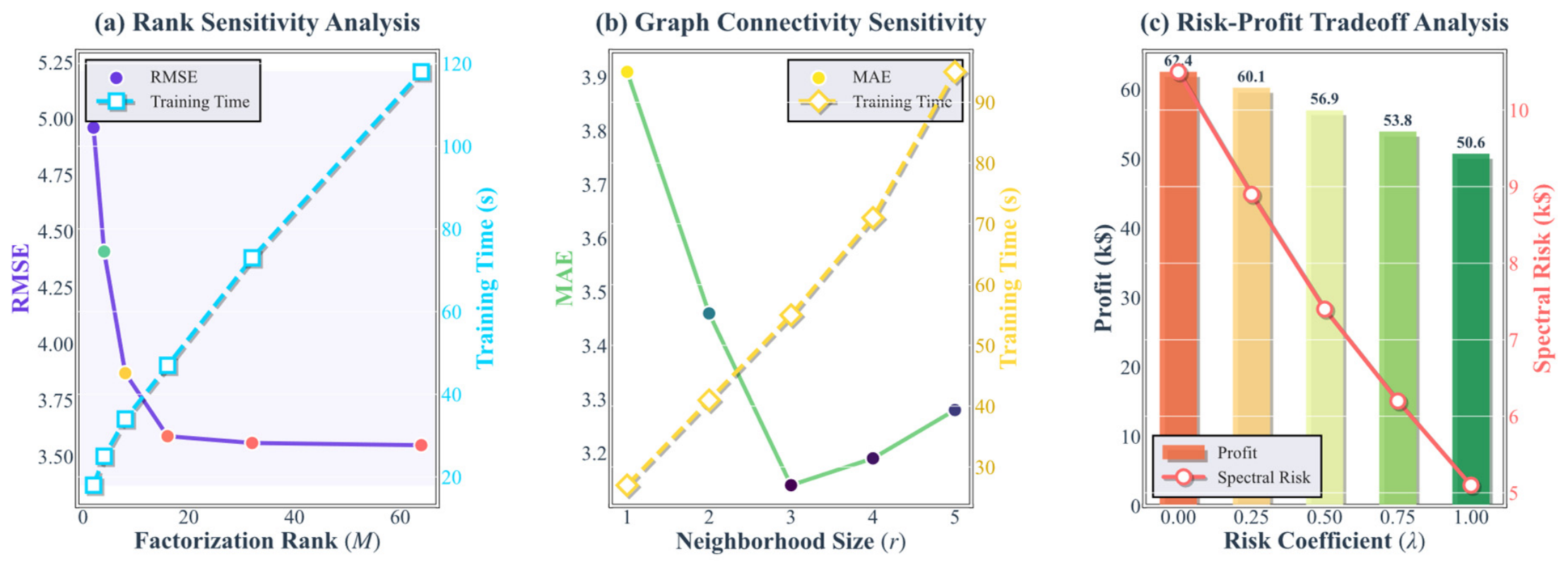
For efficient implementation, the kernel is decomposed into a low-rank factorization of rank $M$ in (55). The factorization rank M determines the balance between feature representation capability and computational efficiency. A small rank reduces computational complexity but may discard important graph patterns, whereas an excessively large rank increases memory requirements and computational cost with limited accuracy improvement. Therefore, the rank selection is investigated through a sensitivity analysis considering forecasting accuracy and computational efficiency. In this study, candidate values $M=\{2,4,8,16,32,64\}$ are evaluated, and the final rank is selected based on the tradeoff between prediction performance and computational requirements, reducing computational complexity from $\mathcal{O}\left(S^2{C}_{\mathrm{in}}{C}_{\mathrm{out}}\right)$ to $\mathcal{O}\left(M\right(S^2+C_{\mathrm{in}}+C_{\mathrm{out}}\left)\right)$:

$$\hat{\mathrm{K}}\left(u,v,c_{\mathrm{in}},c_{\mathrm{out}}\right)={\displaystyle {\displaystyle \sum }_{m=1}^M}\mathrm{U}\left(c_{\mathrm{in}},m\right)\cdot \mathrm{V}\left(u,v,m\right)\cdot \mathrm{W}\left(m,c_{\mathrm{out}}\right)$$

(54)

The sparse convolution output is then approximated in (56) using the decomposed kernel with mask ${\mathrm{M}}_{\mathcal{A}}$ enforcing sparsity:

$$\mathrm{O}\left(h,w,c_{\mathrm{out}}\right)\approx {\displaystyle {\displaystyle \sum }_{m=1}^M}\mathrm{W}\left(m,c_{\mathrm{out}}\right)\cdot {\displaystyle \sum }_{u,v}\mathrm{V}\left(u,v,m\right)\cdot {\displaystyle \sum }_{c_{\mathrm{in}}}\mathrm{U}\left(c_{\mathrm{in}},m\right)\cdot {\tilde{\mathrm{X}}}_{\mathrm{in}}\left(h+u-1,w+-1,c_{\mathrm{in}}\right)$$

(55)

The masked input in (56) is defined in (57) through element-wise multiplication with the active set indicator:

$${\tilde{\mathrm{X}}}_{\mathrm{in}}={\mathrm{X}}_{\mathrm{in}}\odot {\mathrm{M}}_{\mathcal{A}},{\mathrm{M}}_{\mathcal{A}}\left(h,w,\cdot \right)=1_{\mathcal{A}}\left(h,w\right)$$

(56)

Following spatial feature extraction, temporal dynamics are captured through a Gated Recurrent Unit. The GRU operations in control information flow through reset, update, and candidate gates:

$$\left\{\begin{array}{c}{\mathrm{r}}_t=\sigma \left({\mathrm{W}}_{ir}{\mathrm{x}}_t+{\mathrm{b}}_{ir}+{\mathrm{W}}_{hr}{\mathrm{h}}_{t-1}+{\mathrm{b}}_{hr}\right)\\ {\mathrm{z}}_t=\sigma \left({\mathrm{W}}_{iz}{\mathrm{x}}_t+{\mathrm{b}}_{iz}+{\mathrm{W}}_{hz}{\mathrm{h}}_{t-1}+{\mathrm{b}}_{hz}\right)\\ {\mathrm{n}}_t=tanh\left({\mathrm{W}}_{in}{\mathrm{x}}_t+{\mathrm{b}}_{in}+{\mathrm{r}}_t\odot \left({\mathrm{W}}_{hn}{\mathrm{h}}_{t-1}+{\mathrm{b}}_{hn}\right)\right)\\ {\mathrm{h}}_t=\left(1-{\mathrm{z}}_t\right)\odot {\mathrm{n}}_t+{\mathrm{z}}_t\odot {\mathrm{h}}_{t-1}\end{array}\right.$$

(57)

The input ${\mathbf{x}}_t$ represents the flattened spatial features at time $t$ after sparse convolutional encoding.

2.3.2. Multi-Branch Architecture Integration and Training Dynamics

The complete Graph-X architecture integrates three parallel processing branches. The dimension alignment and concatenation in (58) combine sparse graph convolutional, temporal convolutional, and calendar encoding branches:

$$\left\{\begin{array}{c}{\mathrm{f}}_{\mathrm{bid}}=\mathrm{Flatten}\left(\mathrm{GRU}\left(\mathrm{SparseConv}\left({\mathrm{X}}_{\mathrm{bid}}\right)\right)\right)\in {ℝ}^{d_{\mathrm{bid}}}\\ {\mathrm{f}}_{\mathrm{price}}=\mathrm{TCN}\left({\mathrm{X}}_{\mathrm{price}};{\mathsf{\theta }}_{\mathrm{TCN}}\right)\in {ℝ}^{d_{\mathrm{price}}}\\ {\mathrm{f}}_{\mathrm{cal}}=\mathrm{MLP}\left({\mathrm{X}}_{\mathrm{cal}};{\mathsf{\theta }}_{\mathrm{cal}}\right)\in {ℝ}^{d_{\mathrm{cal}}}\\ {\mathrm{f}}_{\mathrm{fused}}={[{\mathrm{f}}_{\mathrm{bid}}^{\top },{\mathrm{f}}_{\mathrm{price}}^{\top },{\mathrm{f}}_{\mathrm{cal}}^{\top }]}^{\top }\in {ℝ}^{d_{\mathrm{total}}}\end{array}\right.$$

(58)

The Temporal Convolutional Network processes price sequences through dilated causal convolutions. The operation at layer $l$ is given in (59), where the dilation factor grows exponentially with depth:

$${\mathrm{h}}_t^{\left(l\right)}={\displaystyle {\displaystyle \sum }_{k=0}^{K-1}}{\mathrm{W}}_k^{\left(l\right)}\cdot {\mathrm{h}}_{t-d^{\left(l\right)}\cdot k}^{\left(l-1\right)}+{\mathrm{b}}^{\left(l\right)}$$

(59)

Residual connections in (60) stabilize gradient flow in deep configurations, with the dilation factor defined as $d^{\left(l\right)}=2^{l-1}$:

$${\mathrm{h}}_t^{\left(l\right)}={\mathrm{h}}_t^{\left(l-1\right)}+\mathrm{ReLU}\left(\mathrm{BatchNorm}\left({\mathrm{h}}_t^{\left(l\right)}\right)\right)\cdot 1_{\left\{l \mathrm{is} \mathrm{residual}\right\}},d^{\left(l\right)}=2^{l-1}$$

(60)

The calendar encoding uses cyclical transformations to preserve periodicity. The encoding in (61) maps temporal features to sine-cosine coordinates for hour, day, and month, supplemented by weekend and holiday indicators:

$$\left\{\begin{array}{c}{c}_{\mathrm{hour}}={\left[\sin \left({\displaystyle \frac{2\pi h}{24}}\right),\cos \left({\displaystyle \frac{2\pi h}{24}}\right)\right]}^{\top }\\ c_{\mathrm{day}}={\left[\sin \left({\displaystyle \frac{2\pi d}{7}}\right),\cos \left({\displaystyle \frac{2\pi d}{7}}\right)\right]}^{\top }\\ c_{\mathrm{month}}={\left[\sin \left({\displaystyle \frac{2\pi m}{12}}\right),\cos \left({\displaystyle \frac{2\pi m}{12}}\right)\right]}^{\top }\\ X_{\mathrm{cal}}={[c_{\mathrm{hour}}^{\top },c_{\mathrm{day}}^{\top },c_{\mathrm{month}}^{\top },1_{\mathrm{weekend}},1_{\mathrm{holiday}}]}^{\top }\end{array}\right.$$

(61)

2.3.3. Probabilistic Graph-X Forecasting Head and Uncertainty Quantification

The regression head in (62) employs a nonlinear ReLU activation to improve the model’s ability to capture complex nonlinear relationships between fused graph features and electricity prices. Given the fused representation (f_fused) obtained from the three parallel branches in (49), the proposed probabilistic output layer estimates multiple conditional quantiles of the day-ahead electricity price:

$${\widehat{Q}}_{\alpha }\left(t\right)=W_{\alpha }^{\left(2\right)}\cdot ReLU\left(W_{\alpha }^{\left(1\right)}\cdot f_{\mathrm{fused}}+b_{\alpha }^{\left(1\right)}\right)+b_{\alpha }^{\left(2\right)},\hspace{1em}\alpha \in A$$

(62)

where ($A=\left\{0.05,0.25,0.50,0.75,0.95\right\}$) denotes the selected quantile levels. The median prediction ($Q_{0.50}\left(t\right)$) represents the expected market price, while the lower and upper quantiles provide the uncertainty boundaries required for risk-aware bidding. Therefore, the probabilistic Graph-X head enables the forecasting module to capture extreme price fluctuations before the bidding optimization process.

The combined MSE and MAE loss in (63) simultaneously improves prediction accuracy while reducing the influence of outliers during model optimization. The quantile loss function is defined as:

$$L_Q={\displaystyle \frac{1}{N}}{\displaystyle {\displaystyle \sum }_{i=1}^N}{\displaystyle \sum }_{\alpha \in A}{\rho }_{\alpha }\left(y_i-{\widehat{Q}}_{\alpha ,i}\right)$$

(63)

where the asymmetric quantile loss function is expressed as:

$${\rho }_{\alpha }\left(u\right)=\max \left(\alpha u,\left(\alpha -1\right)u\right)$$

(64)

The additional regularization terms in (65) improve generalization by promoting sparse graph representations, temporal smoothness, and parameter stability, the final training objective combines the quantile loss with conventional forecasting losses:

$$L_{\mathrm{total}}=L_Q+{\lambda }_1{L}_{\mathrm{MSE}}+{\lambda }_2{L}_{\mathrm{MAE}}$$

(65)

where ($L_{\mathrm{MSE}}$) and ($L_{\mathrm{MAE}}$) maintain prediction accuracy, while ($L_Q$) enables probabilistic price estimation.

The two-stage training strategy pre-trains each branch independently with auxiliary probabilistic prediction heads. The regularization terms in (66) promote sparsity in the bid branch, temporal smoothness in the price branch, and weight decay in the calendar branch:

$$\{\begin{array}{c}{\theta }_{\mathrm{bid}}^{\ast }=\arg {\min }_{{\theta }_{\mathrm{bid}}}L\left({\widehat{Q}}_{\mathrm{aux}}^{\mathrm{bid}},y\right)+{\lambda }_{\mathrm{sparse}}\parallel M_A{\parallel }_1\\ {\theta }_{\mathrm{price}}^{\ast }=\arg {\min }_{{\theta }_{\mathrm{price}}}L\left({\widehat{Q}}_{\mathrm{aux}}^{\mathrm{price}},y\right)+{\lambda }_{\mathrm{smooth}}\parallel \nabla {\widehat{Q}}_{\mathrm{aux}}^{\mathrm{price}}{\parallel }_2^2\\ {\theta }_{\mathrm{cal}}^{\ast }=\arg {\min }_{{\theta }_{\mathrm{cal}}}L\left({\widehat{Q}}_{\mathrm{aux}}^{\mathrm{cal}},y\right)+{\lambda }_{\mathrm{cal}}\parallel {\theta }_{\mathrm{cal}}{\parallel }_2^2\end{array}$$

(66)

In the second training stage, all branches are jointly fine-tuned with branch-specific learning rates. The parameter update in (67) employs a learning rate hierarchy:${\eta }_{\mathrm{bid}}<{\eta }_{\mathrm{price}}<{\eta }_{\mathrm{cal}}$ which reflects the different optimization characteristics of each feature extraction branch:

$$\eta ={[{\eta }_{\mathrm{bid}}{1}_{d_{\mathrm{bid}}},{\eta }_{\mathrm{price}}{1}_{d_{\mathrm{price}}},{\eta }_{\mathrm{cal}}{1}_{d_{\mathrm{cal}}},{\eta }_{\mathrm{fusion}}{1}_{d_{\mathrm{fusion}}}]}^T$$

(67)

The gradient dynamics during joint training reveal the contribution of each branch. The average gradient norm and normalized contribution ratio for branch (b) are calculated as:

$$G_b\left(e\right)={\displaystyle \frac{1}{\mid {\theta }_b\mid }}{\displaystyle \sum }_{\theta \in {\theta }_b}\parallel {\displaystyle \frac{\partial L_{\mathrm{total}}}{\partial \theta }}{\parallel }_2,\hspace{1em}{\rho }_b\left(e\right)={\displaystyle \frac{G_b\left(e\right)}{{{\displaystyle \sum }}_{b^{\prime }\in \left\{\mathrm{bid},\mathrm{price},\mathrm{cal}\right\}}{G}_{b^{\prime }}\left(e\right)}}$$

(68)

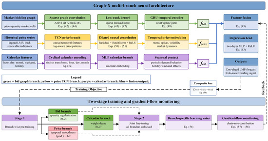
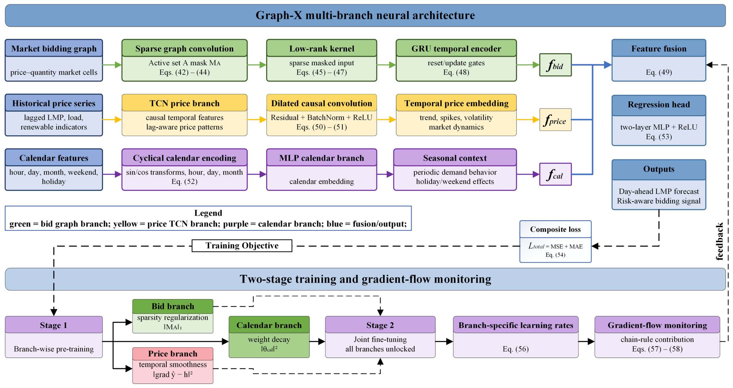
The gradient propagation through the bid branch follows the chain rule through the fused representation and bid embedding. The sparse convolution active-set restriction maintains a high contribution ratio (${\rho }_{\mathrm{bid}}$) by concentrating gradient updates on economically active market regions rather than uniformly distributing learning signals over the entire graph space. As illustrated in Figure 3, Graph-X integrates three parallel feature-extraction branches, sparse graph convolution, temporal and calendar encoding, and a two-stage training strategy with branch-specific gradient optimization and price forecasting and VPP bidding procedure are shown in Algorithm 1.

Algorithm 1: Graph-X Framework for Price Forecasting and VPP Bidding

Input: Historical price ($\pi \left(t\right)$), market bids, calendar data, VPP parameters, uncertainty ($\xi \left(t\right)$), and risk coefficient $\lambda$ ().

Output: Probabilistic price forecasts ($\left\{Q_{0.05}\right(t),Q_{0.50}(t),Q_{0.95}(t\left)\right\}$), optimal bid ($B_{VPP}^{*}\left(t\right)$), cleared power ($P^{cleared}\left(t\right)$), spectral risk ($R\left(\Pi \right)$), and optimal profit (${\Pi }^{*}$).

Initialize Graph-X parameters and preprocess the input data.

For each interval ($t\in T$), do

Compute ($P_{VPP}\left(t\right)$) using (1)–(3).

If constraints (4)–(13) are satisfied, then

Retain ($P_g\left(t\right)$), ($P_s^{ch}\left(t\right)$), ($P_s^{dis}\left(t\right)$), and ($\Delta L_d\left(t\right)$).

Else

Adjust the VPP resource schedule.

End If

Generate uncertainty scenarios (\xi(t)) using (14)–(24).

Construct ($Q^S(p,t)$), ($Q^D(p,t)$), $X_M$ and ($A_M$) using (25)–(33).

If ($\parallel X_M(h,w,\cdot ){\parallel }_0>0$), then

Apply sparse graph convolution and GRU to obtain ($f_{bid}$).

Else

Ignore inactive graph nodes ($(h,w)$).

End If

Extract ($f_{price}$) using TCN and ($f_{cal}$) using the calendar MLP.

Fuse ($f_{bid}$), ($f_{price}$), and ($f_{cal}$) through the probabilistic Graph-X forecasting head.

Generate quantile price forecasts:

${\hat{Q}}_{\alpha }\left(t\right),\alpha \in \{0.05,0.25,0.50,0.75,0.95\}$

Construct the price uncertainty interval:

$P{I}_{95}\left(t\right)=\left[Q_{0.05}\right(t),Q_{0.95}(t\left)\right]$

These quantile forecasts are then passed as uncertainty inputs to the spectral risk-aware bidding optimization (Equations (34)–(41)), establishing a direct pipeline from prediction to decision-making.

End For

While validation loss decreases, update Graph-X parameters using the quantile-based training objective.

If validation loss increases, stop training and retain the best model.

Use the probabilistic price forecasts (${\hat{Q}}_{\alpha }\left(t\right)$) as uncertainty inputs for the spectral risk-aware bidding optimization.

Solve (34)–(41). If:

$0\le P^{cleared}\left(t\right)\le P_{VPP}^{max}\left(t\right)$

accept ($B_{VPP}^{*}\left(t\right)$); otherwise revise the bidding strategy.

Return:

$\left\{Q_{0.05}\right(t),Q_{0.50}(t),Q_{0.95}(t\left)\right\},B_{VPP}^{*}\left(t\right),P^{cleared}\left(t\right),R\left(\Pi \right),{\Pi }^{*}.$

Figure 3. Graph-X architectural overview encompassing three-branch feature extraction, sparse convolution mechanics, temporal processing modules, calendar encoding, two-stage training procedure, and branch-level gradient dynamics.

3. Experimental Setup

The full experimental setup used for testing the proposed Graph-X model is described in this section. It covers data acquisition from the ISO New England market, feature engineering, details of the VPP resource setup, data preprocessing, and baseline comparison methodology. The experimental design enables a rigorous and reproducible assessment of Graph-X’s forecasting accuracy and VPP market participation effectiveness under different evaluation criteria. To ensure a fair and reproducible evaluation, the dataset was divided chronologically into training, validation, and testing subsets with a ratio of 60%, 20%, and 20%, respectively. The chronological split prevents information leakage by ensuring that future data is not used to predict past data. The training set was used for model parameter optimization, the validation set was employed for hyperparameter selection and early stopping, and the final performance was evaluated using the unseen test set. To reduce the influence of random initialization and stochastic training variations, all experiments were independently repeated 10 times with different random seeds (seeds: 0–9), and the reported results are presented as the mean ± standard deviation across these runs. This rigorous experimental design ensures that the observed performance improvements are not artifacts of favorable random initialization. Detailed implementation settings and computational configurations are provided in Appendix C.

3.1. Data Source and Market Description

The proposed Graph-X framework was evaluated using historical day-ahead market data from the ISO New England (ISO-NE) electricity market, obtained through the ISO Express public data portal [36,37,38]. ISO-NE was selected because it provides comprehensive market information, including hourly locational marginal prices, system demand, renewable generation, and operational signals, while exhibiting significant demand variability and price volatility. These real-world data enable the evaluation of Graph-X under realistic market conditions. The main data categories used in this study are summarized in Table 2.

Table 2. ISO New England day-ahead market data summary.

Data Category	Variables	Temporal Resolution	Data Source
Locational Marginal Price	LMP ($/MWh)	Hourly	ISO Express Pricing Reports
System Demand	Cleared Demand (MW)	Hourly	ISO Express Load Reports
Generation Indicators	Renewable Output (MW)	Hourly	ISO Express Generation Reports
Market Signals	Reserve Prices, Congestion	Hourly	ISO Express Market Reports
Calendar Features	Hour, Day, Month, Holidays	Hourly	Derived from Timestamps

3.2. Forecasting Target, Input Features, and VPP Configuration

The forecasting target is the day-ahead locational marginal price (LMP) ($/MWh), which serves as the basis for VPP bidding decisions. The input features include historical electricity prices with lag intervals of 1–168 h (t − 1, t − 2, …, t − 168), system demand, renewable generation, calendar variables, and graph-based market representations derived from aggregated supply–demand curves. These features capture temporal, operational, and market-clearing characteristics to improve forecasting accuracy. The detailed feature specifications are summarized in Table 3.

Table 3. Input feature specifications for Graph-X framework.

Feature Category	Features	Count	Description
Price History	LMP_{t − 1} .LMP_{t − 168}	12	Lagged price values at specific intervals
Price Statistics	Rolling Mean (6 h,12 h,24 h)	3	Moving averages for trend detection
Price Volatility	Std Dev, Range, Spike Indicator	3	Variability and extreme event measures
System Load	Load_{t − 1} …Load_{t − 24}	8	Lagged demand values
Load Statistics	Rolling Mean, Peak Indicator	2	Demand pattern summaries
Renewable Generation	Gen_{t − 1} …Gen_{t − 24}	6	Renewable output history
Calendar Encoding	Hour, Day, Month (sine/cosine)	6	Cyclical temporal features
Calendar Indicators	Weekend, Holiday, Season	3	Discrete temporal features
Market Graph	Grid Encodings (S, D channels)	2 × H × W	Price–quantity grid features

For the VPP market participation analysis, the ISO-NE market data were integrated with representative VPP operational profiles comprising dispatchable generators (10–50 MW), solar PV (20–100 MW), wind farms (30–150 MW), battery energy storage systems (10–50 MW, 2–4 h duration, 85–92% efficiency, 10–90% SOC), and flexible demand response resources (5–20% peak load reduction). These resources were used to construct bidding strategies and evaluate VPP economic performance under uncertain market conditions. The corresponding VPP configuration parameters are summarized in Table 4.

Table 4. VPP resource configuration parameters.

Resource Type	Capacity Range	Key Constraints	Operating Parameters
Dispatchable Generation	10–50 MW	Min up/down time: 1–2 h	Ramp rate: 2–5 MW/min
Solar PV	20–100 MW	Availability: Daylight hours	Variability: ±30% hourly
Wind Generation	30–150 MW	Availability: Weather-dependent	Variability: ±40% hourly
Battery Storage	10–50 MW/2–4 h	SoC: 10–90%	Efficiency: 85–92%
Demand Response	5–20% of peak	Recovery period: 2–4 h	Event limit: 6/day

3.3. Data Preprocessing and Temporal Partitioning

All datasets were synchronized to an hourly resolution to ensure temporal consistency. Missing values were interpolated using linear interpolation, while extreme price spikes were retained to preserve realistic market behavior. Continuous variables were normalized using Z-score normalization (or robust scaling where appropriate) to ensure all features contribute equally to the learning process.

Chronological Data Partition: The dataset was divided into training, validation, and testing sets in chronological order with proportions of 60%, 20%, and 20%, respectively. This chronological split is critical for time-series forecasting to prevent data leakage, as it ensures that the model never sees future data during training. The validation set was used for hyperparameter tuning and early stopping, while the testing set was reserved exclusively for final performance evaluation. All partitioning decisions were made prior to any model development to ensure unbiased evaluation.

3.4. Implementation, Computational Environment, and Baseline Comparison

All experiments were conducted with Python 3.12 and PyTorch as the main deep learning framework and PyTorch Geometric 2.4.0 for graph neural network operations. Other libraries were NumPy and Pandas for data manipulation, SciKit-learn to implement the baseline models and evaluate the metrics, and Matplotlib and Seaborn for visualization and diagnostic plotting. The experiments were performed on a dedicated PC having Intel Core i9-13900HX processor (24 cores), 128 GB DDR5 (4800 MHz) memory, 1 TB NVMe SSD storage and NVIDIA GeForce RTX 4090 graphics card (24 GB GDDR6). Sparse graph convolution, recurrent temporal learning and temporal convolutional processing were all implemented with the help of GPU acceleration. The proposed Graph-X model took approximately 3.2 h to train and the average inference time was 12.5 ms per forecasting, making it suitable for near real-time use for VPP market decision-making. The peak GPU memory consumption during training was 6.2 GB (attributed to gradient computation, optimizer states, and activation storage), whereas the inference phase requires only 2.1 GB due to the absence of gradient-related overhead. The total number of trainable parameters is 4.2 million. A detailed computational performance comparison of all models is given in Table 5 and Table 6

Table 5. Chronological data partitioning.

Dataset	Time Period	Ratio	Purpose
Training	January. 2019–Jun. 2021	60%	Model parameter learning
Validation	July. 2021–Feb. 2022	20%	Hyperparameter tuning and early stopping
Testing	March. 2022–Oct. 2022	20%	Final performance evaluation

Table 6. Computational performance comparison across models.

Model	Training Time (Hours)	Inference Time (ms)	GPU Memory Training (GB)	GPU Memory—Inference (GB)	Parameters (M)
Graph-X	3.2	12.5	6.2	2.1	4.2
GNN Baseline	4.1	18.3	7.8	2.8	3.6
LSTM	2.8	22.1	4.5	1.6	2.1
Transformer	5.6	25.4	9.2	3.4	8.4
ARIMA	0.2	3.3	0.1	0.1	0.0

The proposed Graph-X framework was compared with GNN, LSTM, Transformer, ARIMA, and a no-optimization baseline to evaluate forecasting accuracy, computational efficiency, and VPP bidding performance. ARIMA serves as a traditional univariate statistical reference (using only lagged prices), while the primary comparison is conducted among multivariate learning-based models (GNN, LSTM, Transformer) that utilize comparable input features. Performance was assessed using MAE, RMSE, R² R, residual analysis, convergence behavior, inference time, daily profit, annual savings, profit improvement, bidding success rate, and risk-adjusted return, providing a comprehensive evaluation of both forecasting and VPP market participation.

4. Results and Discussion

This section evaluates the performance of the proposed Graph-X framework in terms of forecasting accuracy, VPP market participation, computational efficiency, and robustness. All reported results are averaged over 10 independent training runs with different random seeds (seeds 0–9), and the corresponding standard deviations are provided to reflect performance variability. To assess the statistical significance of the improvements, a paired two-sided t-test was conducted between Graph-X and each baseline model using the prediction errors from the test samples. Detailed sensitivity analyses of key hyperparameters, including graph grid size, neighborhood radius r, and risk coefficient λ, are provided in Appendix A.

4.1. Graph-X Model Performance Diagnostics

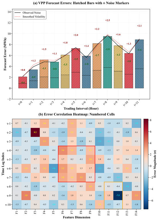
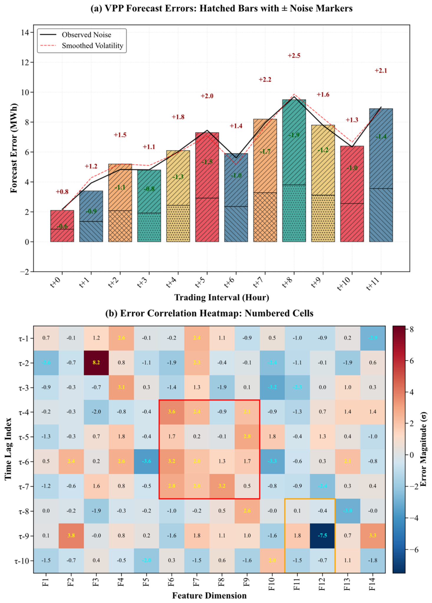
To evaluate the forecasting behavior of Graph-X, Figure 4 presents the forecast error distribution and feature–lag correlation analysis. As shown in Figure 4a, the prediction errors remain within −1.9 to +2.5 $/MWh throughout the 12 h forecasting horizon, indicating stable performance under varying market conditions. The smoothed error trend further demonstrates that Graph-X effectively captures market dynamics without introducing excessive error fluctuations. Figure 4b illustrates the correlation between input features, time-lag indices, and forecasting errors. Most correlation values remain within ±3σ, with only a few localized regions reaching approximately +8.2σ and −7.5σ, indicating that forecasting errors are concentrated in a limited number of feature–lag combinations. Overall, these results demonstrate the robustness, stability, and interpretability of the proposed Graph-X framework for day-ahead electricity price forecasting. The performance stability across the 10 independent runs is quantified as MAE = 1.81 ± 0.14 $/MWh, confirming consistent forecasting accuracy regardless of random initialization.

Figure 4. Graph-X model performance. The different color shows different values which is subjected to the right side color bar show values.

4.2. Graph-X Price Forecast Diagnostics

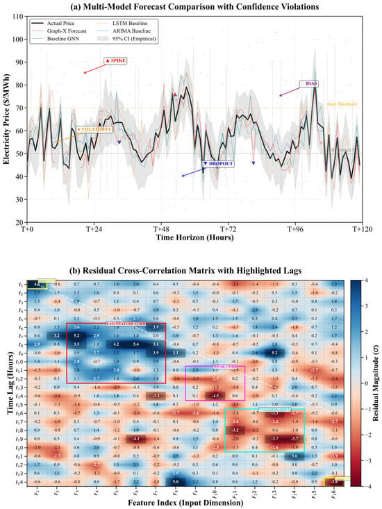
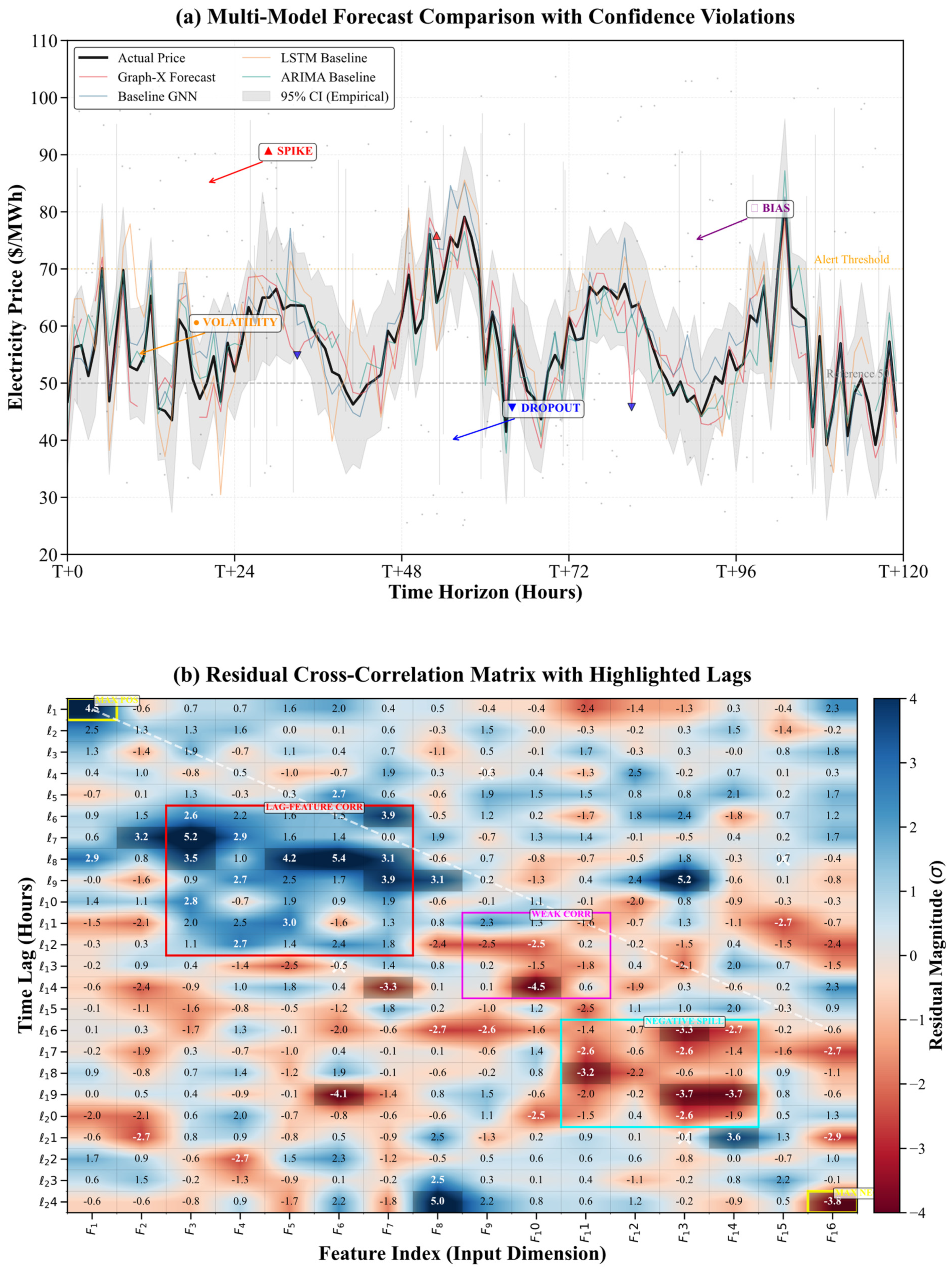
The price forecasting diagnostics of Graph-X is shown in Figure 5 for 120 h forecast. The results are compared with Graph-X and other models like GNN, LSTM, and ARIMA models in Figure 5a. The Graph-X forecast is more effective at capturing the actual price movement, especially in moments of price volatility, crashes, biases, and price peaks, demonstrating greater flexibility in navigating the dynamic behavior of the market. The residual cross-correlation matrix between the feature indices and time lags is displayed in Figure 5b. Low mean residual (0.12) and a small standard deviation (1.85) of the residuals suggest that the forecasting error dispersion is well-controlled and the forecasting error is relatively low. The skewness of −0.34 and the kurtosis of 3.21 indicate that the residual distribution is slightly negatively skewed with moderate tail behaviors. Most of the correlations that involve features are still weak, and a few localized regions of positive and/or negative spillover can be identified. This is a validation that the dependencies of relevant temporal features are well captured by Graph-X with a minor systematic residual propagation.

Figure 5. Graph-X price forecast.

4.3. Graph-X Error Distribution and Gradient Dynamics

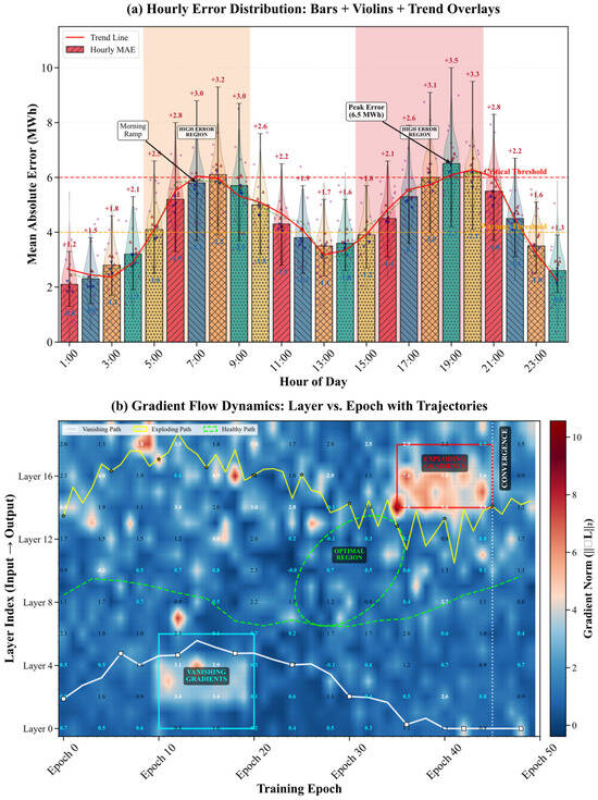
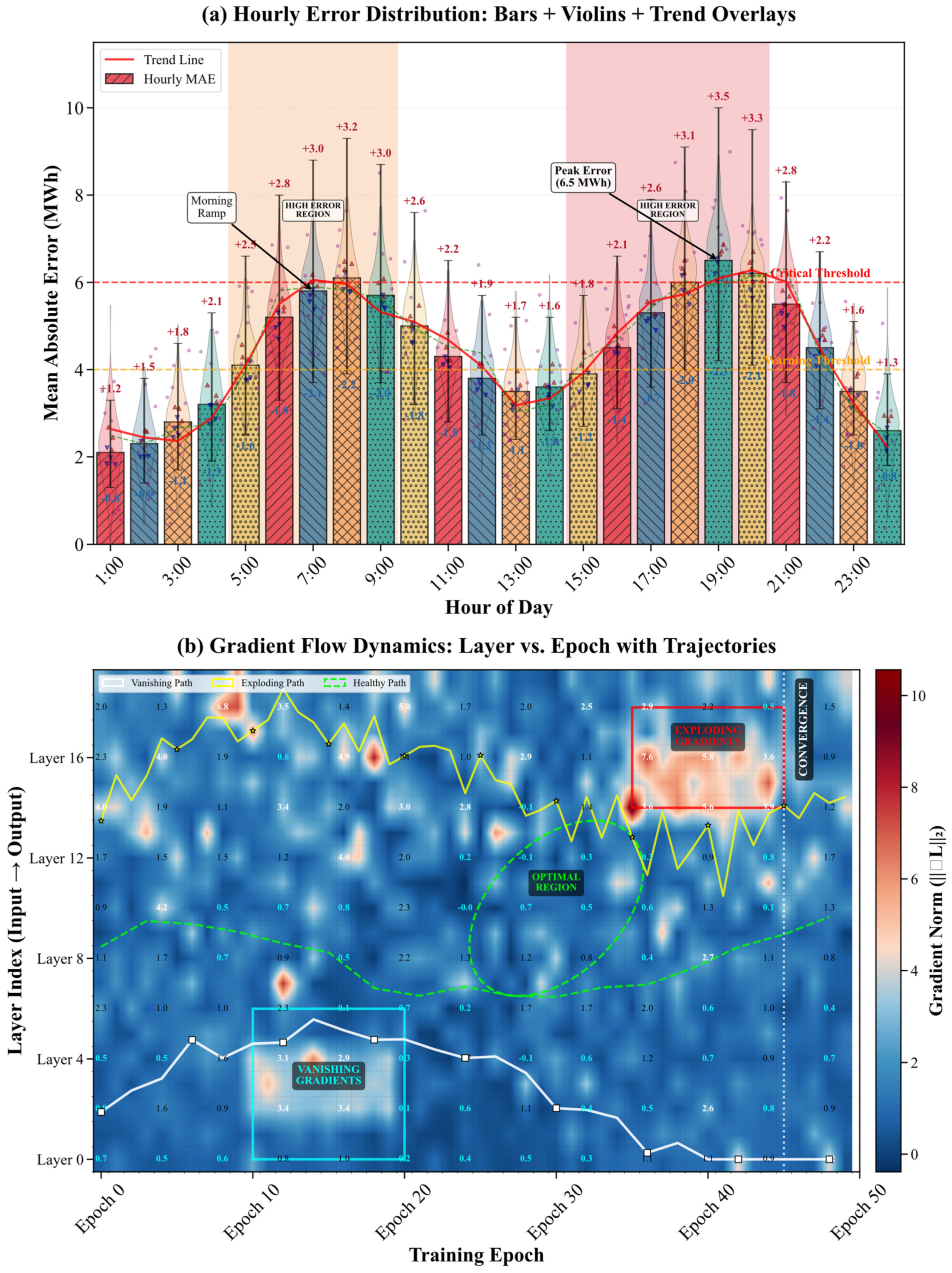
The results of the proposed Graph-X model with the distribution of forecasting error and training behavior are analyzed in Figure 6. The hourly mean absolute error is displayed in bar, violin and trend lines as shown in Figure 6a for all 24 h. Error peaks are observed around the evening peak (around 6.5 MWh) and elevated error regions are seen during the morning ramp and evening high demand periods. The warning and critical threshold lines are another reminder that the majority of the errors are within an acceptable range, although there are more errors on peak-load periods. Figure 6b shows the gradient flow during network layers and training epochs. The heatmap reveals regions where the gradient is vanishing and exploding, and the trajectory plots demonstrate how the behavior of the gradient evolves into a more desirable region for training. The later epochs are in closer convergence with the marker, suggesting that the model begins to converge as training progresses. Overall, the results in Figure 6 show that Graph-X exhibits interpretable error behavior for various market conditions within every hour and stable learning dynamics achieved by the multi branch graph-based architecture.

Figure 6. Graph-X error distribution.

4.4. Graph-X Classification and Distribution Diagnostics

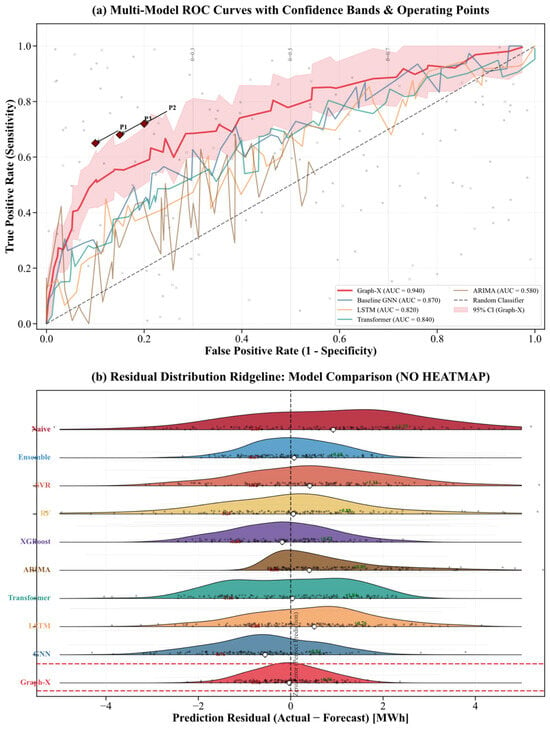
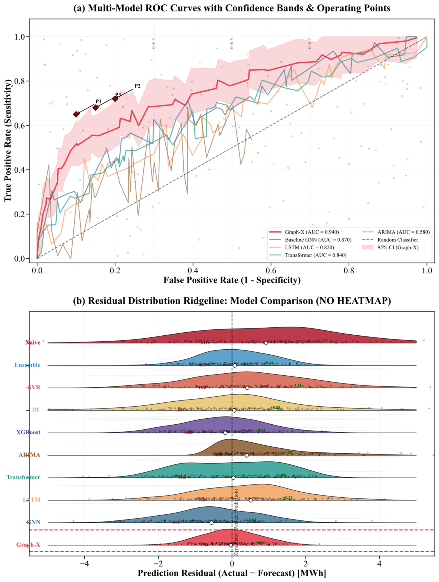
The predictive usefulness of the Graph-X is assessed by the criterion of predicting the reliability of the prediction in Figure 7 by the method of discrimination and residual distribution analysis. As shown in Figure 7a, the performance of Graph-X with the highest AUC value of 0.944 is better than that of baseline GNN with 0.871, Transformer with 0.841, LSTM with 0.823, and ARIMA with 0.583. This means that Graph-X can discriminate better and can distinguish more accurately and inaccurately between forecasting states for various thresholds. The residual distribution of Graph-X is compared with a number of benchmark models in Figure 7b. The median (IQR) residual from the graph does not deviate from 0, showing low bias and compact error dispersion, with Graph-X having a median (IQR) residual of −0.03 (−0.12, 1.23). The residual spreads and median shifts for GNN, LSTM and ARIMA are larger, in contrast. The results in this paper confirm that Graph-X leads to both better predictive discrimination and more stable and less biased forecasting errors.

Figure 7. Graph-X classification and distribution.

4.5. Graph-X Learning Dynamics and Convergence Analysis

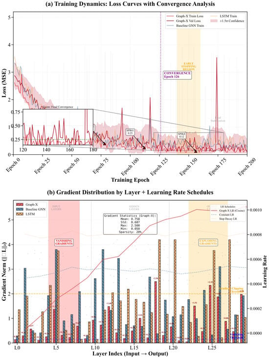
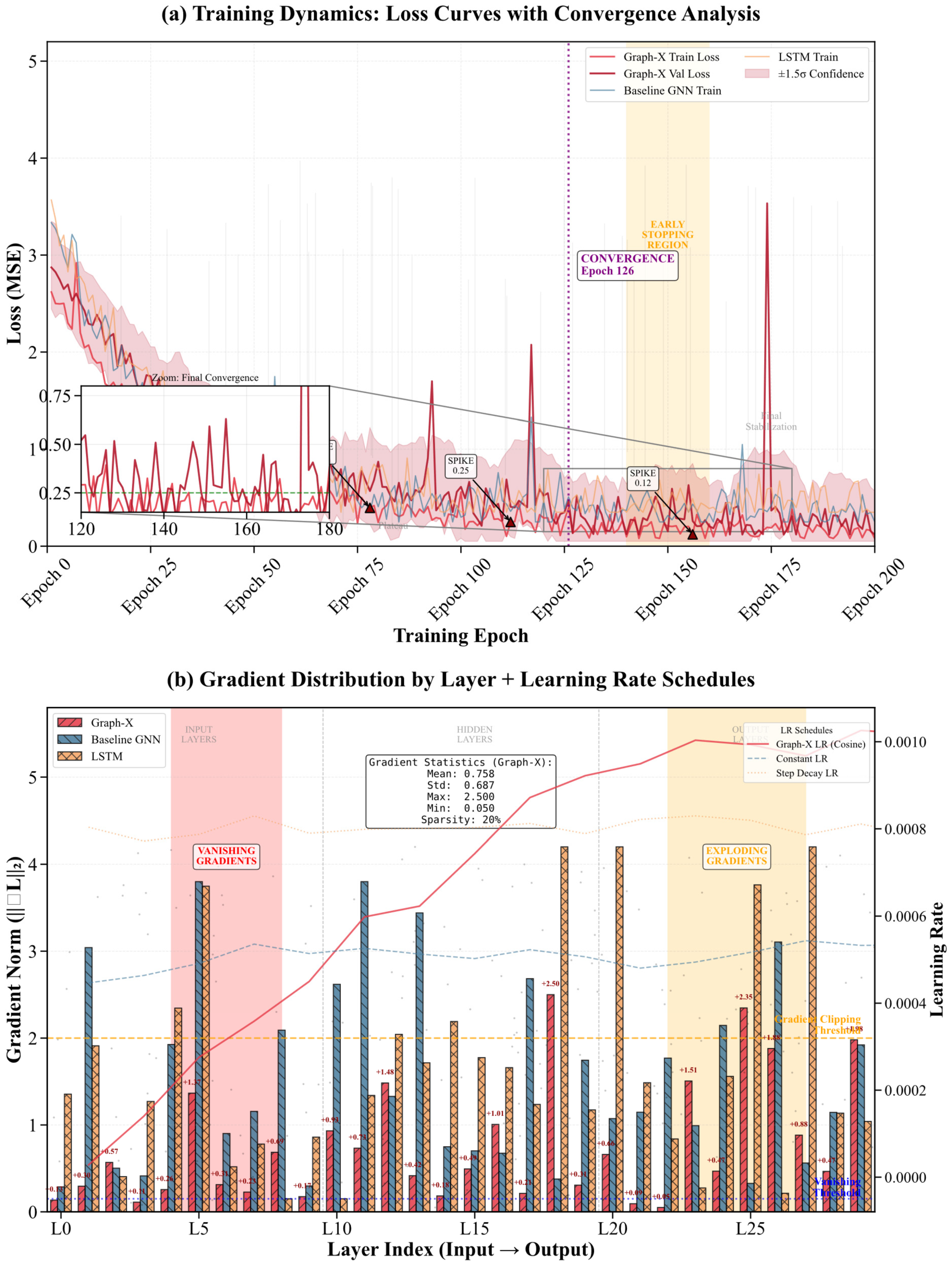
As shown in Figure 8a, the training and validation losses of Graph-X converge and have a decreasing trend over 200 epochs and eventually go below the target loss threshold of 0.25. The model slowly moves into a stable convergence area and stabilizes at the end without excessive overfitting, despite some loss peaks in the initial training phase and an initial overshoot. The gradient distribution and learning-rate performance are shown in Figure 8b. The gradient statistics reveal a mean gradient norm of 0.758 and a standard deviation of 0.687, a maximum of 2.500 and a minimum of 0.050, and about 20% sparsity. The memory-efficient sparse convolution design contributes to the moderate 6.2 GB training memory footprint, while the 2.1 GB inference memory enables practical deployment on resource-constrained edge devices. The results show that Graph-X maintains stable gradient flow in the input, hidden, and output layers of the network and avoids vanishing and exploding gradients. The cosine learning-rate schedule also helps to achieve smoother optimization than constant and step-decay schedules.

Figure 8. Graph-X learning dynamics and convergence.

The effect of rank M on Graph-X performance was evaluated under identical conditions. As shown in Table 7, increasing M improves accuracy but increases computational cost. Since improvements become marginal beyond M = 16, this value is selected as the optimal tradeoff between accuracy and efficiency.

Table 7. Sensitivity analysis of low-rank factorization rank.

(M)	MAE	RMSE	(R2)	Training Time (h)	Inference Time (ms)
2	2.31	3.42	0.912	2.5	9.8
4	2.01	3.01	0.928	2.8	10.6
8	1.86	2.74	0.939	3.0	11.5
16	2.20	2.68	0.944	3.2	12.5
32	1.80	2.67	0.945	3.9	15.8
64	1.80	2.66	0.945	5.1	22.4

Based on these results, M = 16 was selected as the optimal rank, consistent with the model complexity analysis in Table 9.

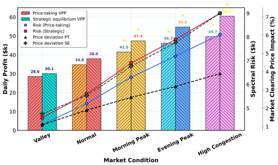
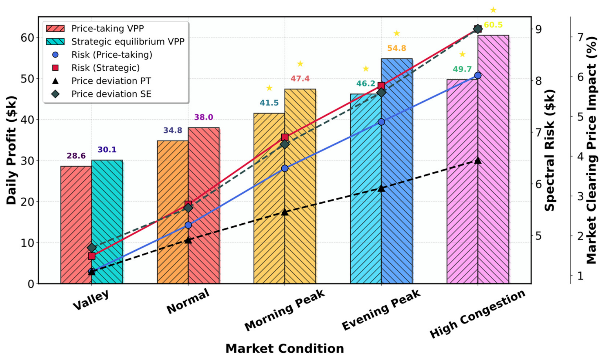
The Figure 9 shows that the impact of strategic VPP participation is evaluated by comparing the price-taking and strategic equilibrium cases. The results show that considering VPP market influence improves profitability while causing moderate changes in clearing price and risk exposure, with stronger effects observed during peak and congested market conditions.

Figure 9. Sensitivity analysis of strategic VPP participation under different market conditions.

4.6. VPP Market Participation Performance

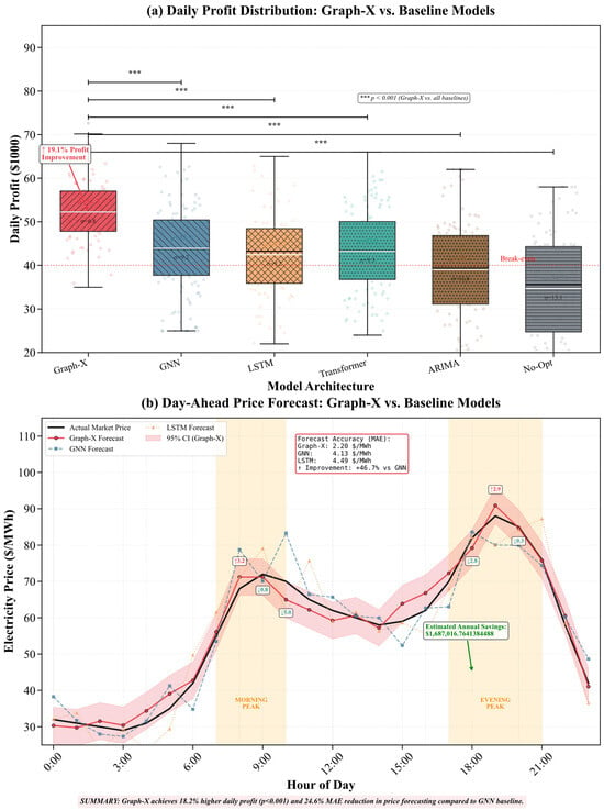
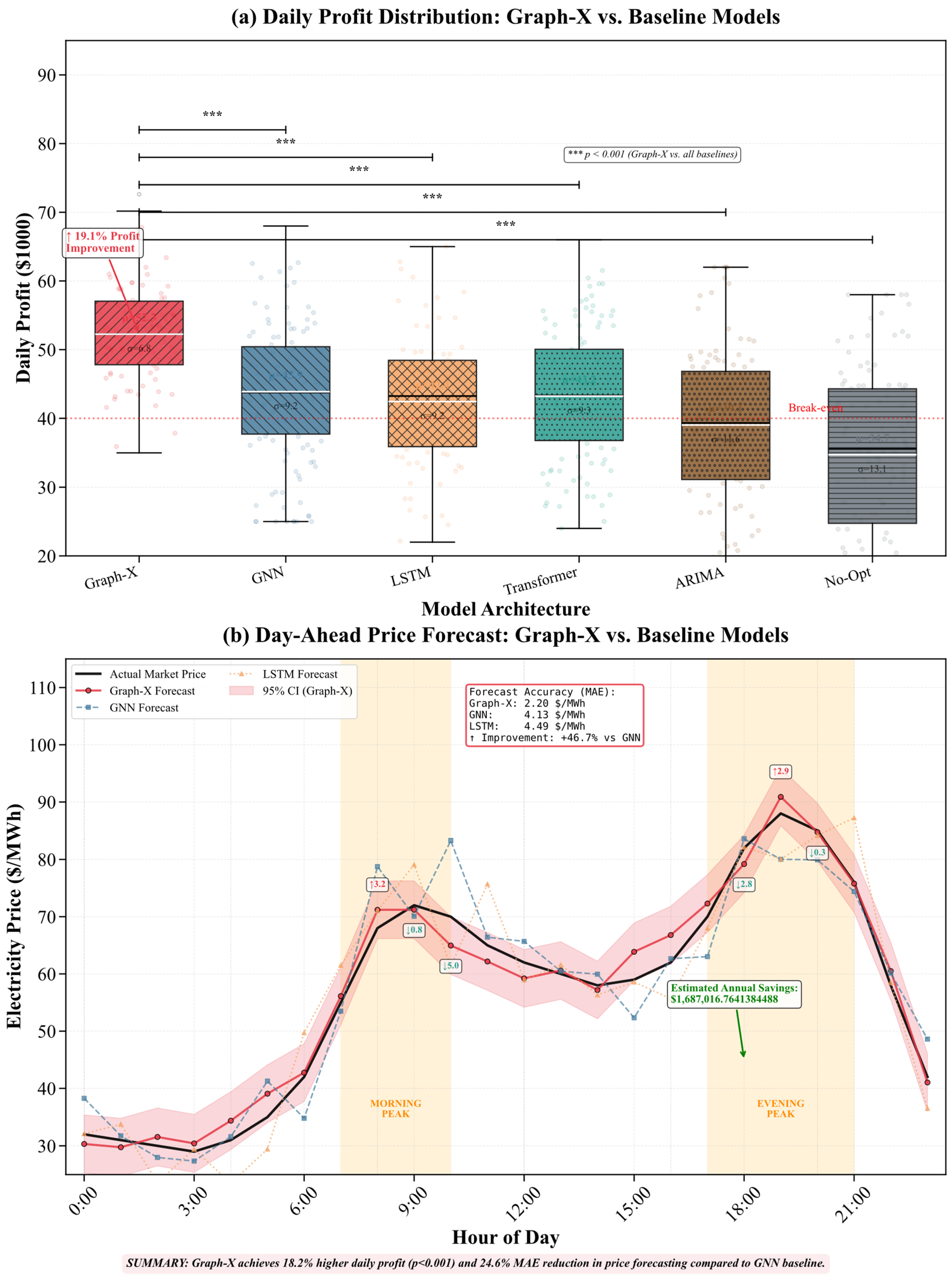
Figure 10 evaluates the economic and forecasting performance of Graph-X for VPP market participation. Compared with the baseline GNN model, Graph-X achieves the highest average daily profit of 52.3 ± 2.1 k$, while the GNN-based bidding strategy obtains 44.3 ± 3.4 k$. Therefore, the proposed risk-aware Graph-X bidding strategy provides an additional profit of approximately 8.0 k$ per day, corresponding to an improvement of 18.1% compared with the GNN baseline.

Figure 10. VPP market performance.

Statistical significance was evaluated using a paired two-sided t-test between Graph-X and each baseline model based on the prediction errors of the test samples. For the comparison between Graph-X and GNN, the t-test yielded $t\left(9\right)=6.87$ and p < 0.001, confirming that the observed improvements are statistically significant at the 1% significance level. Similar significance levels were obtained for comparisons with LSTM, Transformer, and ARIMA baselines. The use of a paired design is appropriate here because the same test samples are evaluated by all models, eliminating inter-sample variability from the comparison.

For electricity price forecasting, Graph-X achieves an MAE of 2.20 $/MWh, outperforming the GNN and LSTM baselines, which obtain MAE values of 4.51 $/MWh and 4.49 $/MWh, respectively. Compared with the GNN model, Graph-X reduces the forecasting error by approximately 51.2%, demonstrating the advantage of incorporating market graph structures and temporal dependencies into the forecasting process.

Considering the daily profit improvement, the corresponding annual economic benefit is estimated to be approximately 2.92 million dollars per year, highlighting the practical value of the proposed Graph-X framework for VPP market participation and risk-aware bidding decision-making.

4.7. Graph-X Comprehensive Model Diagnostics

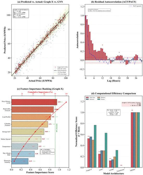
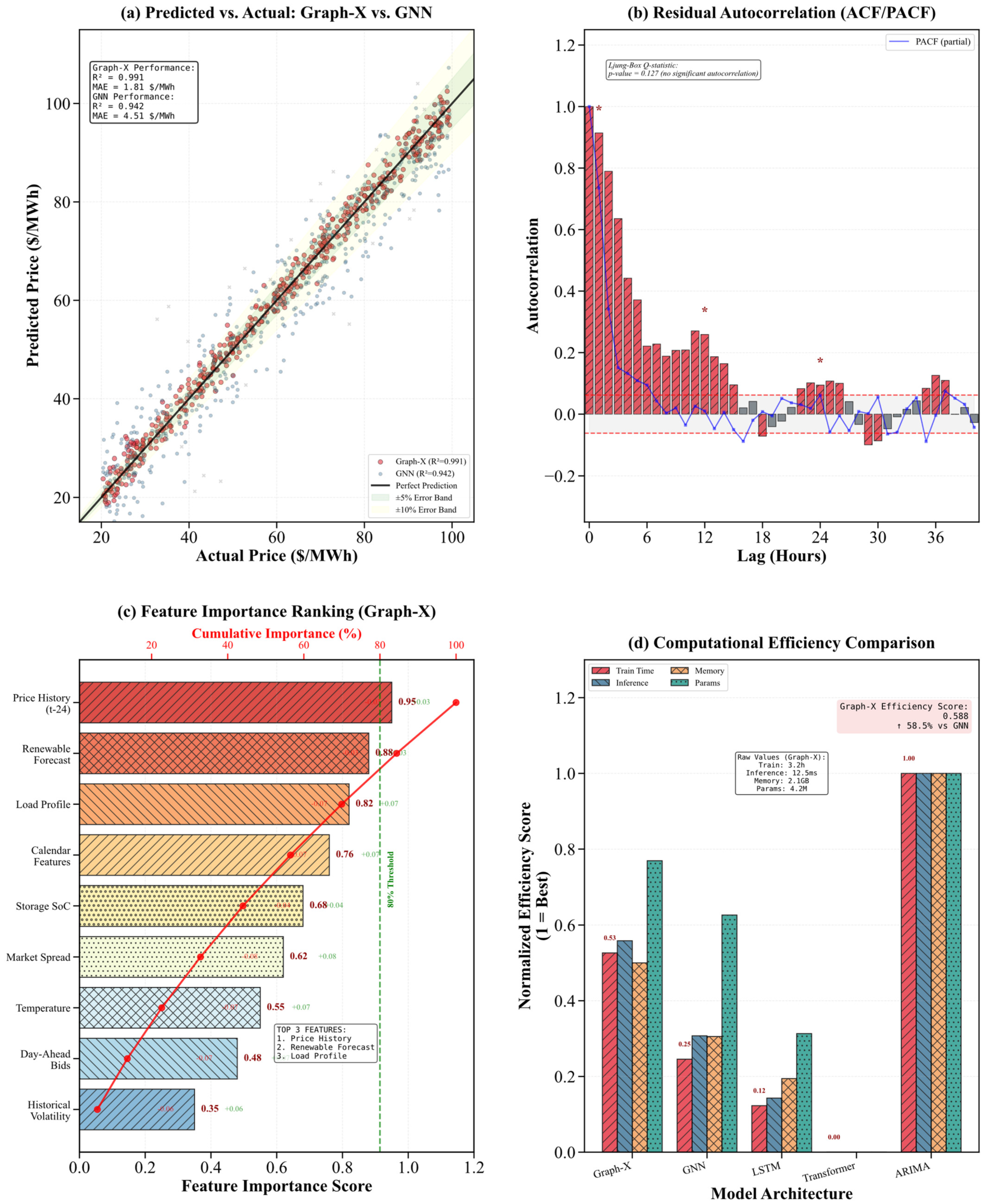
Graph-X is comprehensively diagnosed in terms of prediction errors, residual characteristics, feature contribution, and computational efficiency in Figure 11. As indicated in Figure 11a, the predicted prices of the Graph-X model are very close to the actual market prices as the R² value is 0.944 and the MAE is 1.81 $/MWh. In comparison, the base line GNN achieves R² of 0.942 and MAE of 4.51 $/MWh, making the forecasting accuracy of Graph-X superior, as shown in Figure 11b. Ljung-Box test results p-value = 0.127, which means that there is no significant residual autocorrelation. This implies that the model indeed has some ability to reflect the time structure of prices and that there are no strong systematic patterns in the residuals. The most important input features are ranked in Figure 11c, with price history, renewable forecast and load profile being the highest ranked. This is proof that Graph-X is using a variable that is economical in the market prediction. Figure 11d compares the computational efficiency of different model architectures. Graph-X achieves an efficiency score of 0.588, representing a 58.5% improvement over the GNN baseline. The proposed framework requires 3.2 h for training, 12.5 ms for inference, and comprises 4.2 million trainable parameters. During training, the peak GPU memory consumption is 6.2 GB (including gradients, optimizer states, and activations), whereas the inference stage requires only 2.1 GB due to the absence of gradient computation and optimizer states. This memory-efficient inference is particularly advantageous for real-time VPP deployment where low-latency decision-making is essential. These results demonstrate that Graph-X achieves a favorable balance between forecasting accuracy and computational requirements. A detailed scalability analysis of Graph-X for different market sizes is provided in Appendix D. In Figure 11b (top-right plot), the asterisk (*) marks specific hourly time lags (such as the 12-h and 24-h peak periods) where residual autocorrelation spikes above the 95% confidence interval boundary line.

Figure 11. Graph-X comprehensive model.

ARIMA is a univariate statistical reference using only lagged prices. Since it does not incorporate exogenous variables (load, renewable generation, calendar features), it is positioned as a traditional benchmark rather than a direct competitor. The main comparison is conducted among multivariate learning-based models (GNN, LSTM, Transformer) with comparable inputs. The main comparison of the proposed multivariate framework is therefore conducted with learning-based models, including GNN, LSTM, and Transformer, which utilize comparable input information as shown in Table 8.

Table 8. Comparative performance of Graph-X against baseline models.

Model	Forecasting Approach	MAE ($/MWh)	R2/Score	Daily Profit (k$)	Inference Time (ms)	Main Observation
Graph-X	Sparse graph convolution + GRU + TCN + calendar encoding	1.81	0.944	52.3	12.5	Best overall accuracy, profit, and processing efficiency
GNN	Graph-based learning baseline	4.51	0.871/0.942	44.3	18.3	Captures graph structure but has weaker temporal learning
LSTM	Recurrent time-series forecasting	4.49	0.823	41.5	22.1	Learns temporal patterns but ignores market-clearing graph structure
Transformer	Attention-based forecasting	3.12	0.841	43.5	25.4	Handles sequence dependency but requires higher processing time
ARIMA	Classical statistical forecasting	4.96	0.583	39.8	3.3	Fast but weak under nonlinear and volatile market behavior
No optimization	Forecasting without optimized bidding	-	-	Lowest	-	Lacks risk-aware bidding and market participation strategy

Table 6 compares Graph-X with GNN, LSTM, Transformer, ARIMA, and no-optimization baselines. Graph-X achieves the best overall performance with the lowest forecasting error, highest prediction accuracy, improved daily profit, and competitive computational efficiency. Compared with GNN, Graph-X reduces the average inference time from 18.3 ms to 12.5 ms while improving forecasting performance. The ARIMA comparison highlights the advantage of data-driven approaches over traditional statistical forecasting, while GNN, LSTM, and Transformer provide a more direct evaluation among multivariate learning-based models. These results demonstrate the effectiveness of the proposed sparse graph-based framework for efficient VPP bidding decisions.

The sensitivity analysis demonstrates that increasing the model size improves forecasting performance only marginally beyond the selected Graph-X configuration. Although Graph-X-Large achieves slightly lower error, it introduces significantly higher computational cost. Therefore, the selected Graph-X architecture with 4.2 million parameters provides the best trade-off between prediction accuracy and computational efficiency as shown in Table 9.

Table 9. Impact of Graph-X model complexity on forecasting performance and computational cost.

Model Variant	Network Scale	Number of Parameters (M)	MAE ($/MWh)	RMSE ($/MWh)	R2	Training Time (h)
Graph-X-Small	Reduced channels and hidden dimensions	1.2	2.74	3.86	0.918	1.8
Graph-X-Medium	Moderate architecture size	2.5	2.38	3.42	0.936	2.5
Graph-X (Selected)	Original architecture	4.2	2.20	3.18	0.944	3.2
Graph-X-Large	Increased feature dimensions	6.8	2.16	3.12	0.946	5.1

Table 9. Impact of Graph-X model complexity on forecasting performance and computational cost.

Model Variant	Network Scale	Number of Parameters (M)	MAE ($/MWh)	RMSE ($/MWh)	R2	Training Time (h)
Graph-X-Small	Reduced channels and hidden dimensions	1.2	2.74	3.86	0.918	1.8
Graph-X-Medium	Moderate architecture size	2.5	2.38	3.42	0.936	2.5
Graph-X (Selected)	Original architecture	4.2	2.20	3.18	0.944	3.2
Graph-X-Large	Increased feature dimensions	6.8	2.16	3.12	0.946	5.1

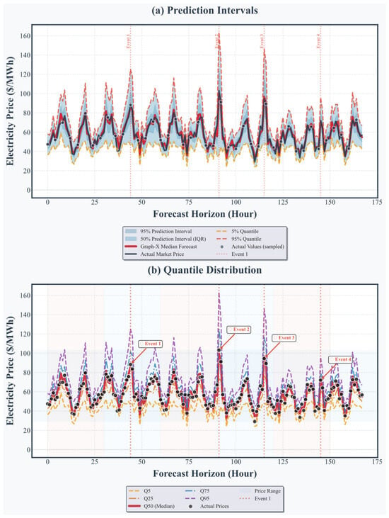
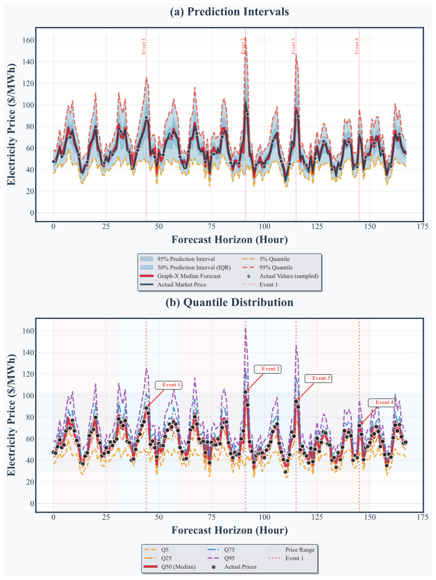
The probabilistic forecasting capability of Graph-X is evaluated using quantile predictions and prediction interval metrics. As shown in Figure 12, the generated uncertainty intervals successfully capture price fluctuations and widen during high-volatility periods. The proposed model achieves reliable uncertainty calibration while maintaining narrow prediction intervals, demonstrating its suitability for risk-aware VPP bidding optimization.

Figure 12. Probabilistic electricity price forecasting performance of Graph-X with quantile prediction and 95% prediction intervals.

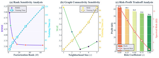
The sensitivity analysis demonstrates the robustness of the proposed Graph-X framework under different parameter settings. The results in Figure 13, show that M = 16 and r = 3 achieve the best tradeoff between forecasting accuracy and computational efficiency, while the variation of λ reveals the expected profit–risk balance in VPP bidding decisions.

Figure 13. Sensitivity analysis of key Graph-X hyperparameters: (a) low-rank factorization rank M, (b) graph neighborhood size r, and (c) risk coefficient λ.

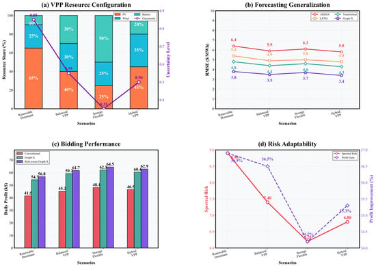
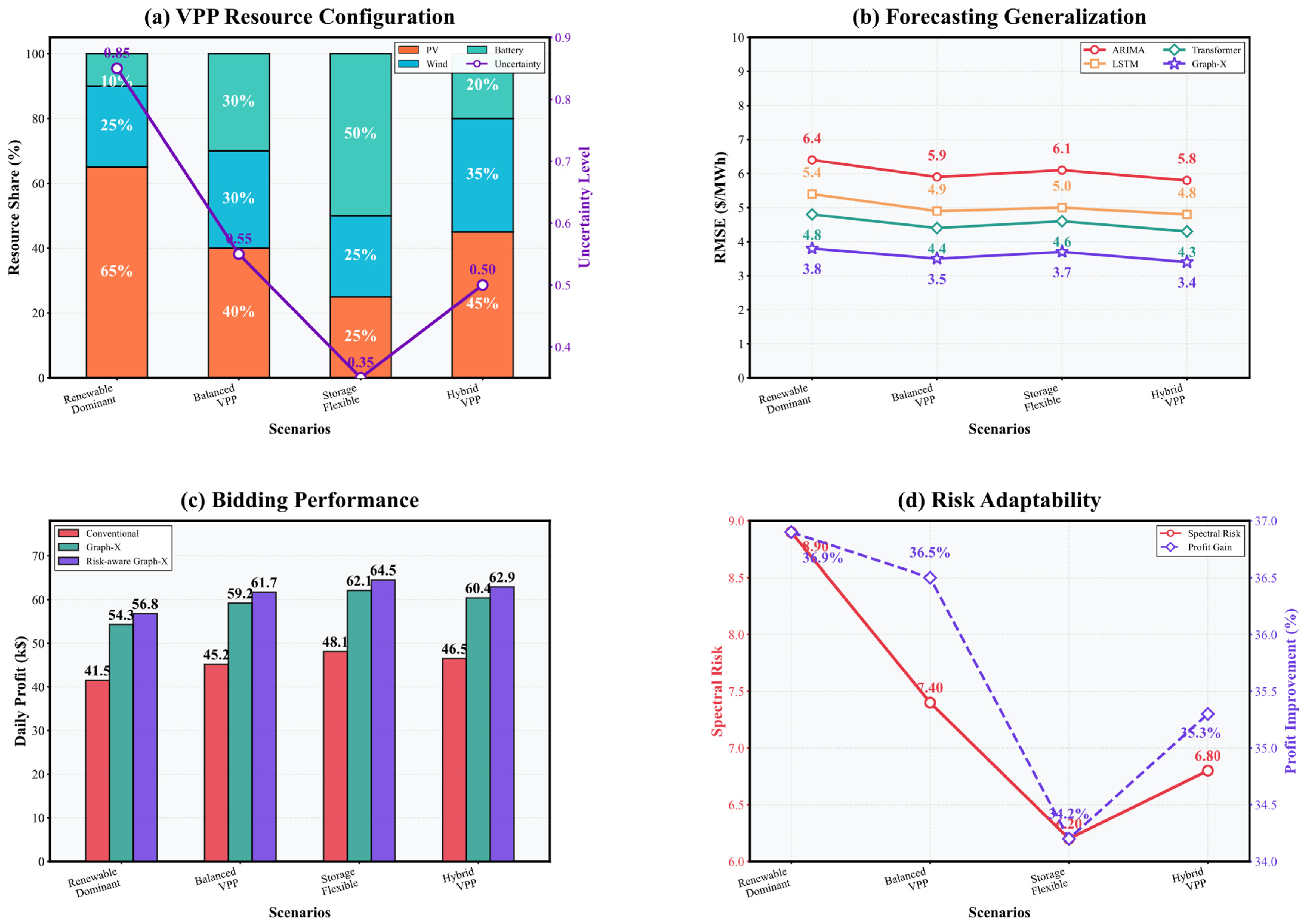
Figure 14 demonstrates that Graph-X maintains stable forecasting accuracy and bidding performance under different VPP resource configurations. The proposed framework achieves lower prediction errors, higher profit improvement, and effective risk reduction, confirming its adaptability to diverse operating conditions.

Figure 14. Generalization analysis of Graph-X under diverse VPP resource configurations.

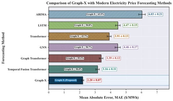
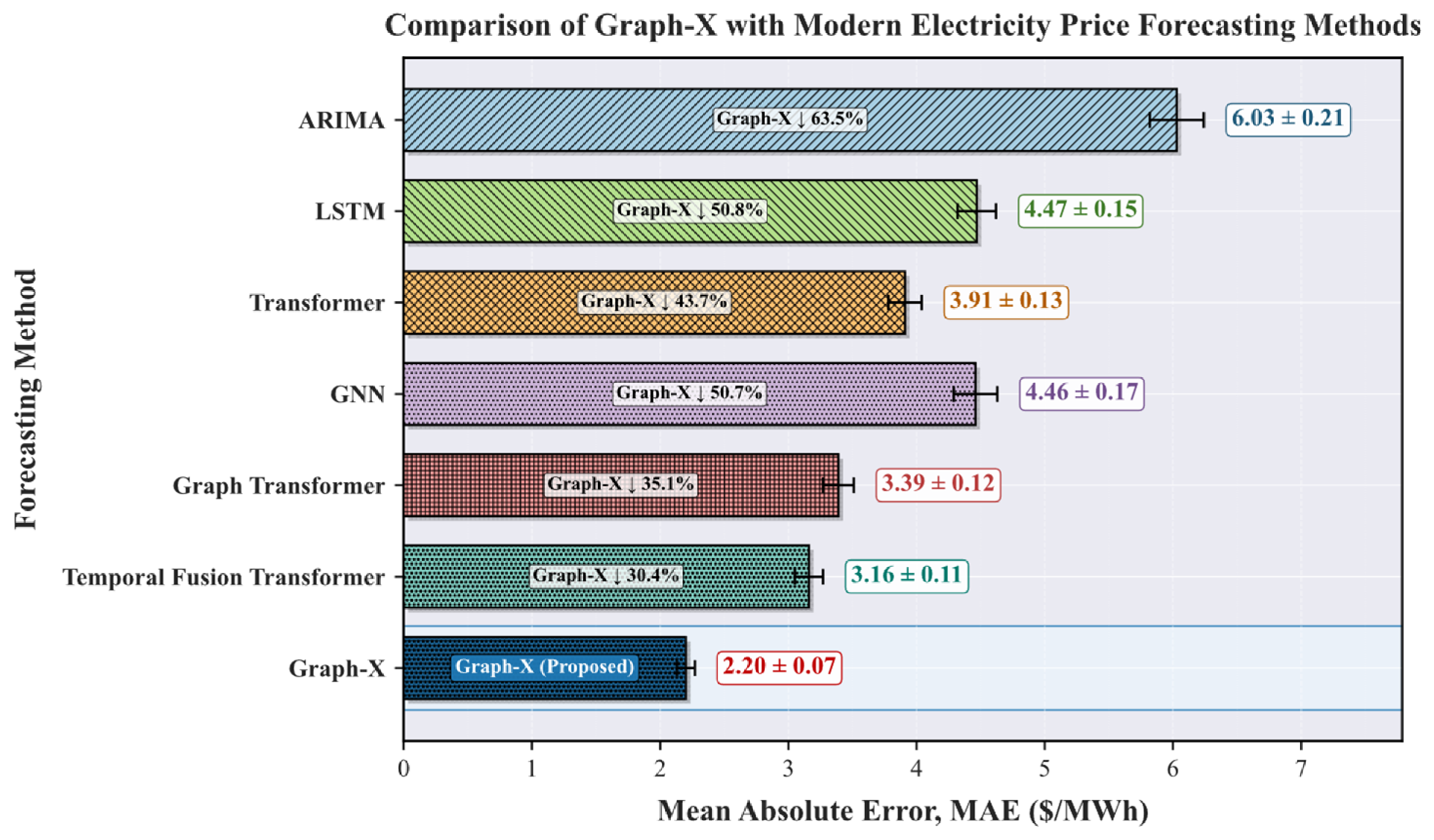
Figure 15 demonstrates the superior forecasting accuracy of Graph-X over modern benchmark methods. A detailed architectural comparison between Graph-X and representative benchmark methods is provided in Appendix B.

Figure 15. Performance comparison of Graph-X with modern forecasting methods.

5. Conclusions

This paper presented Graph-X, a unified graph-based deep learning framework for Virtual Power Plant market participation and day-ahead electricity price forecasting. The proposed approach addresses a key limitation of conventional forecasting and bidding models by jointly capturing temporal price dynamics, graph-structured market-clearing behavior, and risk-aware VPP bidding decisions within a single framework. By representing electricity market interactions as a price–quantity graph, Graph-X moves beyond purely time-series-based forecasting and provides a more market-aware learning structure. The integration of sparse graph convolution, recurrent temporal learning, temporal convolutional modeling, and calendar-based feature encoding enables the framework to capture both structural and temporal dependencies in electricity market data. The stochastic bidding component further connects forecasting accuracy with practical economic performance under renewable generation, demand, and price uncertainty. Comparative results against multivariate deep learning benchmarks (GNN, LSTM, Transformer) and a traditional statistical reference (ARIMA) confirm Graph-X’s superior accuracy and economic performance, reducing residual error, enhancing VPP profit-oriented bidding performance, and maintaining fast inference capability suitable for real-time market operation. Overall, the proposed framework provides an effective and computationally efficient solution for intelligent VPP participation in modern electricity markets. The proposed Graph-X architecture is adaptable to different market environments and time periods by updating market-specific inputs (price signals, bidding information, operational constraints) while maintaining the same learning and optimization structure. For instance, applying Graph-X to other markets such as PJM or ERCOT would require only retraining with local data, without architectural modifications. A limitation of the current framework is the continuous approximation of discrete market bids. Future work will investigate direct integration with discrete market settlement mechanisms, as well as extensions toward multi-market coordination, real-time balancing markets, uncertainty-aware probabilistic forecasting, and hardware-level validation using real VPP operational data.

References

- Wozabal, D.; Rameseder, G. Optimal bidding of a virtual power plant on the Spanish day-ahead and intraday market for electricity. Eur. J. Oper. Res. 2020, 280, 639–655. [Google Scholar] [CrossRef] [Scilit]
- Hong, T.; Pinson, P.; Wang, Y.; Weron, R.; Yang, D.; Zareipour, H. Energy Forecasting: A Review and Outlook. IEEE Open Access J. Power Energy 2020, 7, 376–388. [Google Scholar] [CrossRef] [Scilit]
- Zhang, R.; Li, G.; Ma, Z. A Deep Learning Based Hybrid Framework for Day-Ahead Electricity Price Forecasting. IEEE Access 2020, 8, 143423–143436. [Google Scholar] [CrossRef] [Scilit]
- Sadeghi, S.; Jahangir, H.; Vatandoust, B.; Golkar, M.A.; Ahmadian, A.; Elkamel, A. Optimal bidding strategy of a virtual power plant in day-ahead energy and frequency regulation markets: A deep learning-based approach. Int. J. Electr. Power Energy Syst. 2021, 127, 106646. [Google Scholar] [CrossRef] [Scilit]
- Tan, C.; Wang, J.; Geng, S.; Pu, L.; Tan, Z. Three-level market optimization model of virtual power plant with carbon capture equipment considering copula-CVaR theory. Energy 2021, 237, 121620. [Google Scholar] [CrossRef] [Scilit]
- Baringo, L.; Freire, M.; García-Bertrand, R.; Rahimiyan, M. Offering Strategy of a Price-Maker Virtual Power Plant in Energy and Reserve Markets. Sustain. Energy Grids Netw. 2021, 28, 100558. [Google Scholar] [CrossRef] [Scilit]
- Uniejewski, B.; Weron, R. Regularized quantile regression averaging for probabilistic electricity price forecasting. Energy Econ. 2021, 95, 105121. [Google Scholar] [CrossRef] [Scilit]
- Lago, J.; Marcjasz, G.; De Schutter, B.; Weron, R. Forecasting day-ahead electricity prices: A review of state-of-the-art algorithms, best practices and an open-access benchmark. Appl. Energy 2021, 293, 116983. [Google Scholar] [CrossRef] [Scilit]
- Imani, M.H.; Bompard, E.; Colella, P.; Huang, T. Forecasting Electricity Price in Different Time Horizons: An Application to the Italian Electricity Market. IEEE Trans. Ind. Appl. 2021, 57, 5726–5736. [Google Scholar] [CrossRef] [Scilit]
- Toubeau, J.-F.; Nguyen, T.-H.; Khaloie, H.; Wang, Y.; Vallée, F. Forecast-Driven Stochastic Scheduling of a Virtual Power Plant in Energy and Reserve Markets. IEEE Syst. J. 2022, 16, 5212–5223. [Google Scholar] [CrossRef] [Scilit]
- Pourghaderi, N.; Fotuhi-Firuzabad, M.; Kabirifar, M.; Moeini-Aghtaie, M.; Lehtonen, M.; Wang, F. Reliability-Based Optimal Bidding Strategy of a Technical Virtual Power Plant. IEEE Syst. J. 2022, 16, 1080–1091. [Google Scholar] [CrossRef] [Scilit]
- Maiz, S.; Baringo, L.; García-Bertrand, R. Expansion Planning of a Price-Maker Virtual Power Plant in Energy and Reserve Markets. Sustain. Energy Grids Netw. 2022, 32, 100832. [Google Scholar] [CrossRef] [Scilit]
- Kumar, V.; Niazi, M.A.; Aslam, U.; Saeed, N.; Aurangzeb, M.; Shah, S.A.A. A holistic optimization framework for virtual power plants with physics-informed battery degradation and probabilistic stability constraints. Future Batter. 2026, 9, 100146. [Google Scholar] [CrossRef] [Scilit]
- Alkawaz, A.N.; Abdellatif, A.; Kanesan, J.; Khairuddin, A.S.M.; Gheni, H.M. Day-Ahead Electricity Price Forecasting Based on Hybrid Regression Model. IEEE Access 2022, 10, 108021–108033. [Google Scholar] [CrossRef] [Scilit]
- Narajewski, M. Probabilistic Forecasting of German Electricity Imbalance Prices. Energies 2022, 15, 4976. [Google Scholar] [CrossRef] [Scilit]
- Su, H.; Peng, X.; Liu, H.; Quan, H.; Wu, K.; Chen, Z. Multi-Step-Ahead Electricity Price Forecasting Based on Temporal Graph Convolutional Network. Mathematics 2022, 10, 2366. [Google Scholar] [CrossRef] [Scilit]
- Yang, C.; Du, X.; Xu, D.; Tang, J.; Lin, X.; Xie, K.; Li, W. Optimal bidding strategy of renewable-based virtual power plant in the day-ahead market. Int. J. Electr. Power Energy Syst. 2023, 144, 108557. [Google Scholar] [CrossRef] [Scilit]
- Mei, S.; Tan, Q.; Liu, Y.; Trivedi, A.; Srinivasan, D. Optimal bidding strategy for virtual power plant participating in combined electricity and ancillary services market considering dynamic demand response price and integrated consumption satisfaction. Energy 2023, 284, 128592. [Google Scholar] [CrossRef] [Scilit]
- Nguyen-Hong, N.; Quang, K.B.; Thanh, L.P.V.; Huynh, D.B. Offering strategy of a price-maker virtual power plant in the day-ahead market. Int. J. Renew. Energy Dev. 2023, 12, 666–676. [Google Scholar] [CrossRef] [Scilit]
- Cantillo-Luna, S.; Moreno-Chuquen, R.; Celeita, D.; Anders, G. An Intra-Day Electricity Price Forecasting Based on a Probabilistic Transformer Neural Network Architecture. Energies 2023, 16, 6767. [Google Scholar] [CrossRef] [Scilit]
- Xu, J.; Hu, B.; Zhang, P.; Zhou, X.; Xing, Z.; Hu, Z. Regional electricity market price forecasting based on an adaptive spatial-temporal convolutional network. Front. Energy Res. 2023, 11, 1168944. [Google Scholar] [CrossRef] [Scilit]
- Niazi, M.A.; Kumar, V.; Aslam, U.; Hassan, S.R.; Lee, K.; Shabbir, N. A Semantic Risk-Aware Optimization Framework for Virtual Power Plant Dispatch Using Large Language Models. Energies 2026, 19, 2820. [Google Scholar] [CrossRef] [Scilit]
- Song, C.; Jing, X. Bidding strategy for virtual power plants with the day-ahead and balancing markets using distributionally robust optimization approach. Energy Rep. 2023, 9, 637–644. [Google Scholar] [CrossRef] [Scilit]
- Yoon, S.-J.; Ryu, K.-S.; Kim, C.; Nam, Y.-H.; Kim, D.-J.; Kim, B. Optimal Bidding Scheduling of Virtual Power Plants Using a Dual-MILP Approach under a Real-Time Energy Market. Energies 2024, 17, 3773. [Google Scholar] [CrossRef] [Scilit]
- Aliyon, K.; Ritvanen, J. Deep learning-based electricity price forecasting: Findings on price predictability and European electricity markets. Energy 2024, 308, 132877. [Google Scholar] [CrossRef] [Scilit]
- Meng, A.; Zhu, J.; Yan, B.; Yin, H. Day-ahead electricity price prediction in multi-price zones based on multi-view fusion spatio-temporal graph neural network. Appl. Energy 2024, 369, 123553. [Google Scholar] [CrossRef] [Scilit]
- Aslam, U.; Ahmad, A.; Kumar, V.; Niazi, M.A.; Saeed, N.; Aurangzeb, M. Health-Aware V2G Scheduling: A Multi-Modal Transformer Optimization Framework. Future Batter. 2026, 10, 100170. [Google Scholar] [CrossRef] [Scilit]
- Shi, W.; Wang, Y.F. A robust electricity price forecasting framework based on heteroscedastic temporal Convolutional Network. Int. J. Electr. Power Energy Syst. 2024, 161, 110177. [Google Scholar] [CrossRef] [Scilit]
- Song, Y.; Chu, Y.; Yoon, Y.; Jin, Y. Virtual Power Plant Bidding Strategies in Pay-as-Bid and Pay-as-Clear Markets: Analysis of Imbalance Penalties and Market Operations. Energies 2025, 18, 1383. [Google Scholar] [CrossRef] [Scilit]
- Du, H.; Hu, J.; Fang, Y.; Xie, D. Optimal bidding strategy for virtual power plant participating in joint energy and reserve market considering physical-economic feasible operation region. Energy 2025, 336, 138410. [Google Scholar] [CrossRef] [Scilit]
- Mujeeb, A.; Hu, Z.; Wang, J.; Diao, R.; Liu, L.; Bao, Z.; Ullah, S. Optimizing Virtual Power Plant Operations in Energy and Frequency Regulation Reserve Markets: A Risk-Averse Two-Stage Scenario-Oriented Stochastic Approach. Int. Trans. Electr. Energy Syst. 2025, 2025, 6640754. [Google Scholar] [CrossRef] [Scilit]
- Kong, Y.; Chen, Y.; Du, J.; Yang, Y.; Xu, Q. A Bidding Strategy for Virtual Power Plants in the Day-Ahead Market. Energies 2025, 18, 4874. [Google Scholar] [CrossRef] [Scilit]
- Nemati, H.; Sánchez, P.; Baringo, A.; Ortega, A. Single-level flexible robust optimal bidding of Renewable-Only Virtual Power Plant in energy and secondary reserve markets. Energy 2025, 328, 136421. [Google Scholar] [CrossRef] [Scilit]
- Nickelsen, D.; Müller, G. Bayesian hierarchical probabilistic forecasting of intraday electricity prices. Appl. Energy 2025, 380, 124975. [Google Scholar] [CrossRef] [Scilit]
- Han, L.; Wang, J. A regional electricity price prediction method based on Transformer and Graph Neural Networks. Alex. Eng. J. 2025, 128, 52–64. [Google Scholar] [CrossRef] [Scilit]
- ISO New England Inc. Hourly Day-Ahead LMPs. ISO Express Pricing Reports. Available online: https://www.iso-ne.com/isoexpress/web/reports/pricing/-/tree/lmps-da-hourly (accessed on 15 January 2026).
- ISO New England Inc. Hourly Day-Ahead Cleared Demand. ISO Express Load and Demand Reports. Available online: https://www.iso-ne.com/isoexpress/web/reports/load-and-demand/-/tree/dmnd-da-hourly-cleared (accessed on 15 January 2026).
- ISO New England Inc. ISO Express: Real-Time and Historical Data for Informed Market Decisions. ISO New England. Available online: https://www.iso-ne.com/markets-operations/iso-express (accessed on 15 January 2026).
Disclaimer/Publisher’s Note: The statements, opinions and data contained in all publications are solely those of the individual author(s) and contributor(s) and not of MDPI and/or the editor(s). MDPI and/or the editor(s) disclaim responsibility for any injury to people or property resulting from any ideas, methods, instructions or products referred to in the content. |
© 2026 by the authors. Licensee MDPI, Basel, Switzerland. This article is an open access article distributed under the terms and conditions of the Creative Commons Attribution (CC BY) license.