AJOP-T: A High-Order Hardening Law for Continuous Teardrop Bounding Surface Plasticity

Abstract

Soft-ground finite-element analyses commonly reduce curved Oedometer compression to one constant slope, obscuring where stress-level curvature affects boundary-value predictions. AJOP-T embeds the differentiable Arc Joint via Optimum Parameters map in continuous teardrop bounding-surface plasticity while retaining the inherited yield geometry, non-associated flow, radial mapping and SMP-transformed stress. High-order denotes only the map’s derivative hierarchy: its first two derivatives define tangent hardening and hardening curvature, not gradient, fractional, nonlocal or rate order. This first-phase formulation is deliberately rate-independent and retains constant κ to isolate compression-map hardening; time-dependent and nonlinear cyclic swelling responses are outside its claims. The formulation recovers constant-slope hardening asymptotically, yields a closed-form admissibility boundary, is invariant under SMP, and recovers the parent isotropic normally consolidated settlement equation. Four natural-clay compression maps were fitted; triaxial evidence is fitted for comparison except for one held-out Eastern Osaka extension path. Three implementations agree to at least five significant figures. Paired undrained strip-footing analyses reduce centre settlement by 31.8% in the curved regime but only 0.27% near the high-stress asymptote. A predicted 1.6% low-stress strength-ratio drift is below the reviewed data scatter and is not claimed as experimentally validated.

1. Introduction

Finite-element analyses of soft ground commonly reduce a curved Oedometer compression curve to one constant slope. This is convenient, but natural-clay compression is most curved around the compression-yield transition and only approaches a log-linear asymptote at higher stress. Selecting one compression index therefore selects the stress range in which the approximation is most accurate. The choice is consequential where deep foundations load normally to lightly overconsolidated clay through the transition, tunnel excavation unloads and reloads the surrounding ground across it, and staged preloading or ground improvement is intended to move a deposit through it. The question addressed here is whether the measured curved-to-linear map can be carried into constitutive hardening without changing the remaining plasticity architecture. In the title and throughout this paper, high-order refers only to the compression map and its first two derivatives; it does not denote strain-gradient, fractional, nonlocal or rate-dependent plasticity.

A critical-state plasticity model combines a yield or bounding surface, a plastic flow direction, and a hardening law [1,2,3,4]. Non-associated plasticity separates strength from plastic volumetric flow [5], while stress-dilatancy and plastic-potential relations define the flow direction [6,7]. Modified Cam Clay remains a widely used engineering baseline because its parameters are familiar and its implementation is economical, but its elliptical geometry and constant compression pair restrict the response that can be represented. Generalised yield functions [8,9], continuous teardrop geometry [10], bounding-surface interpolation [11,12,13] and subloading surfaces [14] address different parts of that restriction. The fixed setting adopted here is the continuous teardrop bounding-surface model [10], which combines a smooth two-parameter surface, non-associated flow, radial mapping, a virtual peak stress ratio, and SMP-transformed stress to provide continuous normally consolidated and overconsolidated response. AJOP-T preserves that geometry, flow rule and mapping architecture and changes only the law governing surface growth, allowing paired comparisons with both the parent constant-slope model and Modified Cam Clay to isolate the hardening-law effect.

The compression law that drives hardening has received less attention than geometry and flow. Routine critical-state models generally retain a stress-independent compression slope, and many bounding-surface or subloading extensions refine the interpolation of plastic modulus while leaving that compression pair unchanged. Empirical correlations first linked compressibility to liquid limit and state variables [15,16]; subsequent work established natural-logarithmic compression coordinates [17], distinguished natural-clay sedimentation from intrinsic reconstituted response [18], separated pre-yield, transitional and post-transitional ranges [19], and represented the complete reconstituted-clay curve as S-shaped in e–ln p′ [20]. Nonlinear alternatives also include limiting compression curves for cohesionless soils [21] and explicit structure-dependent laws for clay [22]. Together, these observations show that one constant slope is a local approximation to a compression map whose first derivative varies with stress. The unresolved constitutive question is therefore not whether the curve is nonlinear, but how to embed one differentiable curved-to-linear map so that the measured compression relation and the derivative governing hardening remain mathematically consistent.

The Arc Joint via Optimum Parameters (AJOP) law supplies such a map. It originated in the simplified silty sand model [23] and was later used in a consolidation-settlement procedure driven directly by the Oedometer curve [24]. For the two reported clay examples, replacing the curved-to-linear AJOP description by a linearised description changed the calculated settlement by as much as about 85%; these were method-to-method differences for the same laboratory curves, not errors against field measurements [24]. That study nevertheless showed why both branches matter: a purely curved law cannot recover the high-stress straight branch, whereas one constant slope cannot resolve the transition. The settlement formulation remained one-dimensional and supplied no yield surface, flow direction, consistency condition, stress-point tangent, or evolution rule for unloading, reloading, and shear. Its extension to a constitutive hardening law is therefore a distinct problem rather than a relabelling of the settlement equation.

AJOP-T denotes this constitutive construction: AJOP identifies the new hardening law and T the inherited teardrop-bounding surface [10]. The AJOP map is treated as a differentiable relation between logarithmic preconsolidation stress and void ratio. Its first derivative defines the tangent compression modulus used by the consistency condition, and its second derivative measures the curvature controlling how rapidly that modulus evolves. The resulting derivative hierarchy replaces one constant compression slope while retaining the inherited yield geometry, plastic potential, radial mapping, and SMP transformation. The formulation establishes the high-stress constant-slope limit, a closed-form admissibility boundary, the elasto-plastic tangent, invariance of the hardening hierarchy under the SMP transformation and exact recovery of the parent settlement equation under isotropic normally consolidated loading. The hierarchy is required to exist throughout the interior admissible domain; its limiting behaviour as the boundary is approached is identified analytically and guarded numerically. Calibration uses the ordinary Oedometer or isotropic consolidation curve rather than a new test type, so the additional compression parameters describe the observed curve instead of adding an independent mechanism.

Two control assumptions isolate AJOP compression hardening: a rate-independent soil skeleton and constant κ. They are phase boundaries, not claims that time effects or nonlinear swelling are negligible. Rate means strain rate or any loading-rate variable tied to explicit time, viscosity or a reference rate; none appears in AJOP-T. Sensitive clays show rate coupling [25], and modern formulations represent creep, relaxation, rate-dependent strength, anisotropy or destructuration [26,27,28,29]; AJOP-T is not their substitute. Rate independence limits time-dependent predictions, not load reversals. Constant κ and no cyclic internal variable separately restrict this phase to monotonic and single unload–reload paths, not repeated-cycle hysteresis. Adding either mechanism would require new calibration and confound paired attribution to compression hardening. Destructuration is outside scope. Section 6 and Section 7 bound these effects; evidence is labelled fitted or held out, and neither field validation nor a discretisation-consistent algorithmic tangent is claimed.

Three objectives organise the paper: to derive the AJOP hardening hierarchy and its admissible limits; to embed it without altering the inherited teardrop geometry and SMP mapping while recovering the parent constant-slope and settlement results; and to determine where the substitution produces a measurable constitutive or boundary-value response. The evidence combines closed-form analysis, three execution paths including one independent implementation, material-point calculations, comparisons with Modified Cam Clay and the parent constant-slope model, compression calibrations for four natural clays, fitted and held-out triaxial paths, overconsolidated checks, parameter and constant-swelling-index sensitivities, near-boundary tests and paired strip-footing calculations. The footing problem is an idealised comparative boundary-value verification, not a field settlement prediction. Section 2, Section 3, Section 4 and Section 5 present the inherited framework, AJOP hierarchy, consistency equations, transformation properties and recovery results; Section 6 reports the response maps and data-anchored checks; Section 7 discusses mathematical interpretation, implementation, engineering scope and limitations; Section 8 concludes, and Appendix A collects notation (

Table A1. Principal symbols, physical meanings, sources and roles in the formulation.

Symbol	Definition and Units	Obtained from	Admissible Range and Role
e	void ratio [dim.]	measured	e > 0; state
e0	void ratio at the initial stress [dim.]	measured or initialised from the fitted AJOP map, as stated for each analysis	e0 > 0; initial state
Γ	intercept of the AJOP compression map [dim.]	least squares on the compression curve	>max e; AJOP map
ac	half the asymptotic compression slope [dim.]	least squares on the compression curve	>0; AJOP map
θc	roundness of the transition [dim.]	least squares on the compression curve	>0; θc = 0 is only a nonsmooth limiting case; AJOP map
p′r	reference stress locating the transition [kPa]	least squares on the compression curve	>0; AJOP map
λ∞	asymptotic compression slope, = 2ac [dim.]	derived from ac	>κ; hardening law
λA(u)	tangent compression modulus [dim.]	first derivative of the AJOP map	κ < λA < λ∞; hardening law
κ	swelling index [dim.]	unload–reload branch of the Oedometer test	0 < κ < λ∞; elastic law
ν	Poisson ratio [dim.]	assumed or measured	0 ≤ ν < 0.5; elastic law
M; Me	TC critical-state ratio M; positive SMP-implied TE magnitude Me [dim.]	M from TC; Me from the SMP mapping	>0; signed extension plots use −Me
Ψ	shape exponent of the teardrop surface [dim.]	stress-path shape	>1; base surface
Ω	size parameter of the teardrop surface [dim.]	stress-path shape	>0; base surface
u	hardening coordinate, = ln(P0/p′r) [dim.]	current preconsolidation size	u > u*; hardening law
u*	admissibility boundary of Proposition 1 [dim.]	closed form in ρκ and θc	Derived boundary; domain of validity
ΛA	normalised tangent modulus, = λA/λ∞ [dim.]	derived	0 < ΛA < 1; position on the transition
ρκ	swelling ratio, = κ/λ∞ [dim.]	derived	0 < ρκ < 1; admissibility
P0	preconsolidation size of the bounding surface [kPa]	initial state and hardening	>0; hardening law
p′	mean effective stress [kPa]	state	>0; state
$\stackrel{\sim }{\mathrm{q}}$	deviator stress in SMP transformed stress [kPa]	state and SMP transform	≥0; base surface
$\stackrel{\sim }{\mathrm{\eta }}$	transformed stress ratio, = $\stackrel{\sim }{\mathrm{q}}$/p′ [dim.]	derived	≥0; not globally bounded by M for OC states; base surface
R	spacing ratio of the radial mapping rule [dim.]	current state and image point	0 < R ≤ 1; mapping rule
HA	plastic hardening modulus [kPa−1]	consistency condition	sign follows Mk − $\stackrel{\sim }{\mathrm{\eta }}$; hardening/softening modulus in the elasto-plastic tangent

Note: * denotes the admissibility-boundary value defined in Proposition 1; u* is given by Equation (26).

) and experimental metadata (

Table A2. (a). Material, index, water-state and initial-stress metadata for the literature datasets used in Figure 10, Figure 11, Figure 12 and Figure 13. (b). Test conditions, data use, evidential role and quantitative comparison.

(a)
Dataset/Source	Material, Indices and Water State	Initial Stress/OCR
Boom Clay: Ess75, Ess83, Ess96, Ess104, Ess112 and Mol [39]	Sampling/material: Natural cores. Essen: Putte and Terhagen members, 218.91–256.93 m. Mol: HADES, 223 m. Five Essen cores plus one Mol core. Indices: Essen: Gs 2.64–2.68; LL 62–78%; PL 25–33%; PI 36–45%; initial e 0.700–0.785. Mol: Gs 2.67; LL 59–83%; PL 22–28%; PI 9.5–40%; initial e 0.49–0.67. Water state: Essen: w 26.5–29.7%; Sr 0.97–1.00. Mol: w NA-D; Sr 1.00.	In-situ σ′v0 (MPa): 2.20, 2.27, 2.40, 2.48, 2.56 and 2.23 respectively. OCR is not assigned: [39] warns that the Oedometer yield stress is stress-path dependent and can underestimate the preconsolidation stress.
Eastern Osaka clay, Tsurumi [33]	Sampling/material: Natural sensitive clay; block/cylindrical samples from 8.3 m depth. Clay/silt/sand = 44/49/7%; sensitivity 14.5. Indices: Gs 2.67–2.703; LL 69.2–75.1%; PL 24.5–27.3%; PI 41.9–50.6%. Water state: Natural w 65–72%; Sr NA-D.	Reference mean effective stress σ′m0 = 98 kPa; stress-controlled isotropic yield pressure Pc = 93.1 kPa. A single field OCR is not reported for the digitised record.
Shanghai clay, layer 4 [40]	Sampling/material: Undisturbed sensitive marine clay. The source identifies layer 4 as normally to lightly overconsolidated and reports that its natural structure remains relatively stable after one-dimensional consolidation and drained triaxial testing. Indices: LL, PL/PI and Gs: NA-D. Water state: Natural w and Sr: NA-D.	Published yield knee ≈ 90–100 kPa. σ′v0 and OCR: NA-D. The first digitised point is approximately (σ′v, e) = (12 kPa, 1.145) (D), which is an analysis-start ordinate and not a reported in-situ state.
Weathered Bangkok (Nong Ngoo Hao) clay [41]	Sampling/material: Natural tube samples; dark-grey, fissured weathered clay. Sand/silt/clay = 7.5/23.5/69%; organic matter 4%. Indices: Gs 2.73; LL 123 ± 2%; PL 41 ± 2%; PI 82 ± 4%; natural e 3.86 ± 0.15. Water state: Natural w 133 ± 5%; Sr 95 ± 2%.	Four triaxial specimens were prepared in the nominally normally consolidated range at p′0 = 103, 207, 276 and 414 kPa (D from 15, 30, 40 and 60 psi plotted in source Figure 8). The source notes that the 15 psi specimen may retain slight overconsolidation.
(b)
Test Series	Test Conditions, Start State and Data Used	Evidential Role and Quantitative Comparison
Boom Clay, high-pressure Oedometer [39]	Control/drainage/rate: Drained high-pressure Oedometer; 50 mm diameter × 20 mm specimens; synthetic pore water. Incremental σ′v = 0.125–32 MPa. Deformation stabilised at a displacement rate below 0.01 mm/h. Analysis-start state: Before saturation, all Oedometer specimens were brought to σ′v = 2.40 MPa for testing convenience, although the core-specific in-situ values differ (Table A2(a)). Data used: Nfit = 6 curves × 9 first-loading-envelope ordinates = 54 (current digitisation record).	Role: Compression-map calibration for each core. Not an independent validation dataset. Comparison: RMS(e) = 3.7–7.7 × 10−3. The published compression index and high-stress tangent comparison is an external scalar consistency check, not a held-out curve validation.
Eastern Osaka, KSS5-1 isotropic consolidation [33]	Control/drainage/rate: Stress-controlled drained isotropic consolidation in a triaxial cell; each load step held for 24 h. Average axial strain rate ≈ 2.54 × 10−4%/min. Analysis-start state: First digitised ordinate e ≈ 1.91 at p′ ≈ 10 kPa (D). Published Pc = 93.1 kPa. Data used: Nfit = 9 digitised ordinates (Figure 11a).	Role: Compression-map calibration. Not independent validation. Comparison: RMS(e) = 4.5 × 10−3; fitted p′r = 91.6 kPa against published Pc = 93.1 kPa (independent scalar check).
Eastern Osaka, TSK-6, -2, -3, -8, -9 compression [33]	Control/drainage/rate: Isotropically consolidated undrained triaxial compression; axial strain rate 1.00 × 10−2%/min. Analysis-start state: p′0 (kPa, D): 19.6, 58.8, 117.6, 176.4, 235.2. Source initial specimen e: 1.90, 1.91, 1.91, 1.91, 1.91. Nominal OCR at the start of shear (D): 4.75, 1.58, 1, 1, 1. Data used: Ncurve = 5 digitised compression paths.	Role: Ψ and Ω calibrated by grid sweep on these compression paths. These are therefore fitted comparisons, not validation. Comparison: Path-shape misfits of 0.5–0.7% of p′0 for the two highest-pressure tests, and 15–31% strength underprediction near yield.
Eastern Osaka, TS6-2 extension [33]	Control/drainage/rate: Isotropically consolidated undrained triaxial extension; axial strain rate 6.14 × 10−3%/min; bedding angle 90°. Analysis-start state: p′0 = 117.6 kPa (D); source initial specimen e = 1.68; nominal OCR at the start of shear = 1 (D). Data used: Ncheck = 1 digitised extension path.	Role: Held-out prediction: no extension-side data were used to calibrate Ψ, Ω or Me, and Me is implied by the transformed stress. Comparison: The only genuinely held-out stress-path check in the present dataset.
Shanghai layer 4, one-dimensional Oedometer [40]	Control/drainage/rate: Drained one-dimensional consolidation on an undisturbed specimen. Loading schedule and rate: NA-D. Analysis-start state: First digitised ordinate ≈ (12 kPa, 1.145) (D); published yield knee ≈ 90–100 kPa. Data used: Nfit = 15 digitised ordinates over ≈ 12–2200 kPa (D from Figure 11b).	Role: Compression-map calibration. Not independent validation. Comparison: RMS(e) = 4.3 × 10−3; fitted p′r = 91.2 kPa against the published yield knee of ≈ 90–100 kPa (scalar consistency check).
Weathered Bangkok, isotropic consolidation [41]	Control/drainage/rate: Stress-controlled drained consolidation. Saturation and initial consolidation were simultaneous; specimens were held for 1–5 days to reach 95% consolidation. Analysis-start state: Natural e = 3.86 ± 0.15 and Sr = 95 ± 2%. Specimen-specific analysis-start state: NA-D. Data used: digitised fit ordinates retained; count unavailable (Nfit = NA-D).	Role: Compression-map calibration. Not independent validation. Comparison: RMS(e) = 23.3 × 10−3.
Weathered Bangkok, four nominally normally consolidated undrained triaxial paths [41]	Control/drainage/rate: Stress-controlled undrained shear at constant cell pressure. The exact shearing rate is not reported in [41]. Analysis-start state: p′0 = 103, 207, 276 and 414 kPa. Model-start e0 from the fitted compression map (D): 2.534, 2.024, 1.812 and 1.513; these are not measured specimen values. Data used: Ncurve = 4. The calibration objective was evaluated at 25 common deviator levels per path, giving 100 resampled objective ordinates rather than 100 independent measurements.	Role: Ψ and Ω calibrated to these paths. Figure 13 is therefore a fitted model–data comparison, not independent validation. Comparison: RMS path-shape misfit 1.9% of p′0; strength endpoints within ±8% of p′0.

Notes: Source-reported initial void ratios for the Osaka TSK and TS6 specimens refer to the initial specimen and not automatically to the void ratio at the start of shear used by the model. Reference [41] contains an internal inconsistency: the prose gives the highest normally consolidated undrained consolidation pressure as 50 psi, whereas source Figure 8 and the digitised series show 60 psi; the analysis uses 60 psi, that is 414 kPa. NA-D means unavailable in the digitised analysis record and not necessarily absent from the original paper.

).

2. Base Bounding Surface Framework

AJOP-T retains the transformed stress, teardrop loading and bounding surfaces, plastic potential, radial mapping and virtual peak stress ratio of Chatwong et al. [10]; Section 3 replaces only the hardening law. This section fixes the inherited notation needed later rather than rederiving the base model; full derivations and calibration guidance are given in [10].

2.1. SMP Transformed Stress

Ordinary stress invariants impose deviatoric symmetry and cannot represent clay’s lower triaxial-extension strength. The SMP transform supplies this asymmetry by rescaling deviatoric stress at fixed mean stress. A symmetric surface in transformed variables therefore distinguishes compression from extension without changing compression calibration; Section 5.1 proves this invariance.

Models in $p$ and $q$ imply Extended Mises strength and overpredict clay strength on the $\pi$-plane. Following [10], the SMP criterion [30], used in clay plasticity [31], enters through the SMP-revised Cam-clay transform [32]:

$${\tilde{\sigma }}_{ij}=\tilde{p}\hspace{0.17em}{\delta }_{ij}+{\tilde{s}}_{ij}=p\hspace{0.17em}{\delta }_{ij}+{\displaystyle \frac{q_{\mathrm{S}\mathrm{M}\mathrm{P}}}{q_c}}\hspace{0.17em}{s}_{ij}$$

(1)

where ${\delta }_{ij}$ is the Kronecker delta, $p$ and $s_{ij}$ are the mean and deviatoric parts of ${\sigma }_{ij}$, and

$$q_{\mathrm{S}\mathrm{M}\mathrm{P}}=\sqrt{{\displaystyle \frac{2}{3}}}\hspace{0.33em}{\displaystyle \frac{2I_1}{3\sqrt{\left(I_1{I}_2-I_3\right)/\left(I_1{I}_2-9I_3\right)}-1}}$$

(2)

$$q_c=\sqrt{s_{kl}\hspace{0.17em}{s}_{kl}}$$

(3)

where $I_1$, $I_2$ and $I_3$ are the invariants of ${\sigma }_{ij}$. All subsequent relations use $\tilde{p}={\tilde{\sigma }}_{ii}/3$, $\tilde{q}=\sqrt{\left(3/2\right)\hspace{0.17em}{\tilde{s}}_{ij}{\tilde{s}}_{ij}}$ and $\tilde{\eta }=\tilde{q}/\tilde{p}$; compressive stresses and strains are positive. For triaxial plots only, extension is displayed with a negative signed ordinate; the transformed invariants $\tilde{q}$ and $\tilde{\eta }$ used in the constitutive equations remain non-negative.

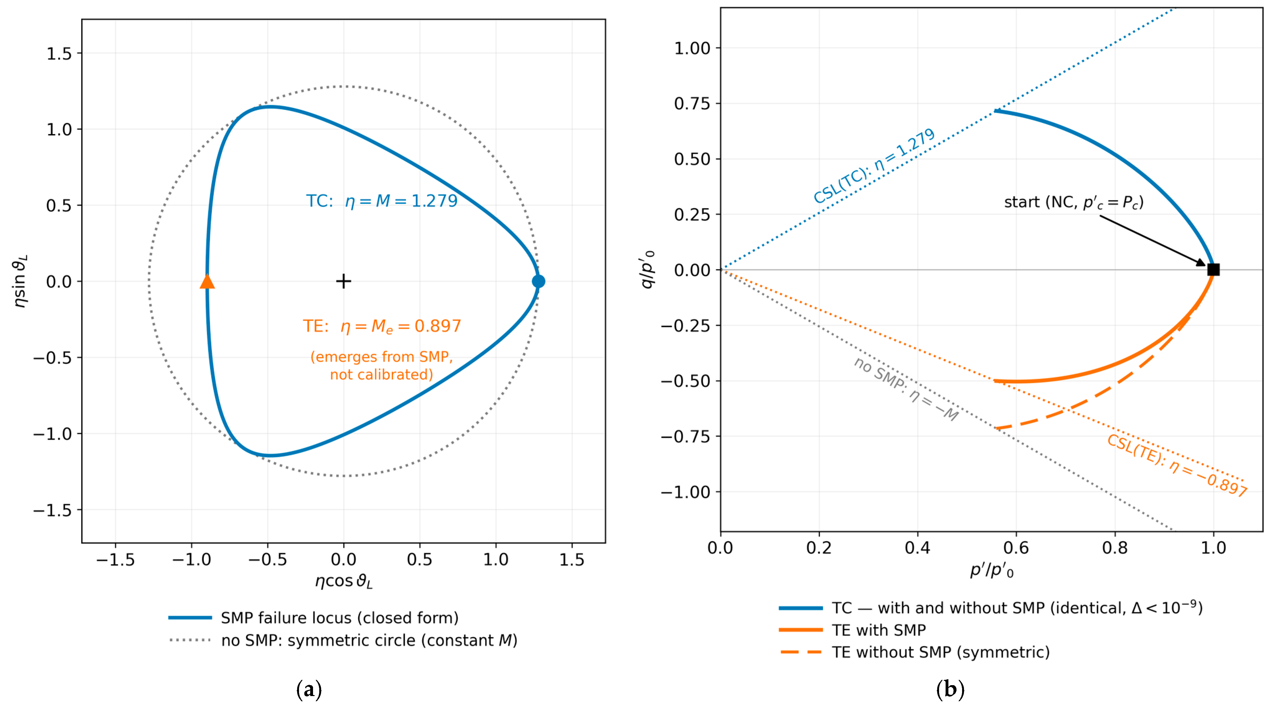
Figure 1 isolates the mapping effect. The SMP locus and symmetric constant-slope circle coincide in triaxial compression but separate in extension, where the critical-state slope is reduced by the Mohr–Coulomb ratio. Reintegrating the same Eastern Osaka material point with the transformed and ordinary deviatoric invariants leaves the compression paths identical to within 10⁻⁹ but changes the extension endpoint by 43%. The transform therefore corrects extension without altering compression-calibrated response; Remark 3 gives the structural proof.

2.2. Bounding Surface, Plastic Potential and Mapping Rule

For image point ($\tilde{P}$, $\tilde{Q}$), preconsolidation size ${\tilde{P}}_0$ and critical-state ratio $M$, the continuous teardrop surface is [10]

$$F=\mathrm{l}\mathrm{n} \left[{\left({\displaystyle \frac{\tilde{P}}{{\tilde{P}}_0}}\right)}^{\Omega }\right]+{\left({\displaystyle \frac{\tilde{\eta }}{M}}\right)}^{\Psi }=0$$

(4)

Here $\Psi$ controls skewness and fits NC stress paths to data—a key feature of [10]; $\Omega$ adjusts strength. The nested loading surface shares this shape; its potential follows [10]

$$g=\mathrm{l}\mathrm{n} \left({\displaystyle \frac{\tilde{P}}{{\tilde{P}}_g}}\right)+{\displaystyle \frac{\tilde{\eta }}{M}}=0$$

(5)

where ${\tilde{P}}_g$ sets the potential size. Radial mapping from $\left(\tilde{p},\tilde{q}\right)$ to $\left(\tilde{P},\tilde{Q}\right)$ gives

$$R={\displaystyle \frac{\mathcal{l}}{L}}={\displaystyle \frac{\tilde{p}}{\tilde{P}}}={\displaystyle \frac{\tilde{q}}{\tilde{Q}}}$$

(6)

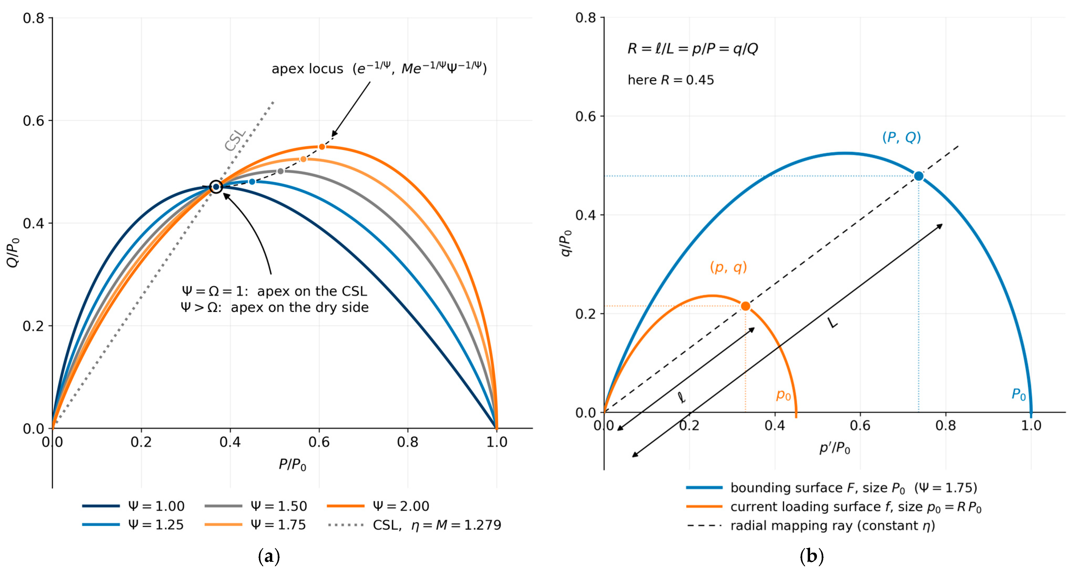
Thus $R=1$ at the bounding surface (NC) and $R<1$ inside it (OC). Figure 2 illustrates the isolated effect of Ψ and the radial mapping rule.

The consistency gradients are

$${\displaystyle \frac{\partial F}{\partial \tilde{P}}}={\displaystyle \frac{1}{\tilde{P}}}\left(\Omega -\Psi {\left({\displaystyle \frac{\tilde{\eta }}{M}}\right)}^{\Psi }\right)$$

(7)

$${\displaystyle \frac{\partial F}{\partial \tilde{Q}}}={\displaystyle \frac{\Psi }{M\tilde{P}}}{\left({\displaystyle \frac{\tilde{\eta }}{M}}\right)}^{\Psi -1}$$

(8)

$${\displaystyle \frac{\partial F}{\partial {\tilde{P}}_0}}=-{\displaystyle \frac{\Omega }{{\tilde{P}}_0}}$$

(9)

2.3. Flow Rule and Sign Conventions

The plastic strain increment is non-associated, $d{\mathsf{\epsilon }}^p=d\Lambda \hspace{0.17em}\mathbf{m}$, with the flow direction obtained from the explicit potential of Equation (5) evaluated at the image point:

$$m_v={\displaystyle \frac{\partial g}{\partial \tilde{P}}}={\displaystyle \frac{1}{\tilde{P}}}\left(1-{\displaystyle \frac{\tilde{\eta }}{M}}\right), m_d={\displaystyle \frac{\partial g}{\partial \tilde{Q}}}={\displaystyle \frac{1}{M\tilde{P}}}$$

(10)

With compression positive, $m_v>0$ on the wet side ($\tilde{\eta }<M$, contractive plastic flow and hardening), $m_v=0$ at the critical state, and $m_v<0$ on the dry side ($\tilde{\eta }>M$, dilative plastic flow and softening). This sign convention fixes the sign of the hardening modulus in Section 4 and is stated here explicitly because every admissibility statement below depends on it. The resulting stress–dilatancy relation is linear:

$$D={\displaystyle \frac{d{\epsilon }_v^p}{d{\epsilon }_d^p}}={\displaystyle \frac{m_v}{m_d}}=M-\tilde{\eta }$$

(11)

2.4. Base Hardening Law and Plastic Modulus

This subsection is the one the paper replaces, so it is worth isolating what it does. The bounding surface grows as plastic volumetric strain accumulates, and how fast it grows is governed by a single number: the difference between the compression slope and the swelling slope. In the base model, that number is a constant, because the compression curve is taken to be a straight line. Everything from Section 3 onward follows from letting it vary with stress instead.

In the base model, the bounding surface size evolves with the plastic volumetric strain through the constant compression index $\lambda$ and swelling index $\kappa$ of the log-linear idealisation:

$$d{\tilde{P}}_0={\tilde{P}}_0\hspace{0.17em}{\displaystyle \frac{1+e_0}{\lambda -\kappa }}\hspace{0.17em}d{\epsilon }_v^p$$

(12)

The plastic modulus interpolated for OC states replaces $M$ by the virtual peak stress ratio $M_k$ of Dafalias and Herrmann [12]:

$$K_p={\displaystyle \frac{1+e_0}{\lambda -\kappa }}\left(M_k-\tilde{\eta }\right){\displaystyle \frac{\partial g}{\partial \tilde{Q}}}$$

(13)

$$M_k=M{R}^{-n}$$

(14)

so that $M_k=M$ on the bounding surface and $M_k>M$ inside it. The interpolation exponent $n$ follows the OCR-dependent relations of [10],

$$n=0.5+{\displaystyle \frac{2}{\mathrm{O}\mathrm{C}\mathrm{R}}} (\mathrm{undrained} \mathrm{loading})$$

(15)

$$n=0.5+M^2+{\displaystyle \frac{2}{\mathrm{O}\mathrm{C}\mathrm{R}}} (\mathrm{drained} \mathrm{loading})$$

(16)

Remark 1 (calibration input under AJOP hardening).

The correlations for  $\Psi$  and  $\Omega$ in [10] take the plasticity measure $\lambda -\kappa$ as input, and Equations (15) and (16) were calibrated under the constant-$\lambda$ idealisation. When the AJOP hierarchy of Section 3 replaces $\lambda$, the corresponding input is the asymptotic difference  $2a_c-\kappa$, which Equation (22) identifies as the high-stress limit of  ${\lambda }_A-\kappa$. This choice keeps all inherited correlations well defined and reduces to the original definitions exactly in the log-linear limit.

3. AJOP Hardening Hierarchy

AJOP-T’s sole substitution requires a differentiable compression map. Section 3.1 defines it, Section 3.2 derives its first two derivatives, and Section 3.3 recovers the classical constant-slope high-stress limit without adding a physical assumption.

3.1. Compression Map

The AJOP law [24] maps a logarithmic hardening coordinate to void ratio. Define

$$u=\mathrm{l}\mathrm{n} \left({\displaystyle \frac{{\tilde{P}}_0}{p_r}}\right)$$

(17)

where $p_r>0$ marks the curved-to-linear transition; in factored form,

$$e_A\left(u\right)=\Gamma -a_c\left(u+\sqrt{{\theta }_c+u^2}\right)$$

(18)

Here $\Gamma$ is the low-stress asymptote, $a_c>0$ the asymptotic half-slope, and ${\theta }_c>0$ the transition roundness. $R$ denotes the Equation (6) mapping ratio; ref. [24] uses $R$ for reference stress.

Remark 2 (conversions).

Equation (18) is [24] in natural-log form: $a_c$ =  $\alpha$ and  ${\theta }_c={\theta }_P/{\alpha }^2$, where ${\theta }_P$ is the [24] roundness. Thus, multiply the fitted ${\theta }_c$ values by  ${a_c}^2$ for the [24] convention. The dimensionless $u$ uses the natural logarithm. If  $a_c$ is obtained from $C_c$ per decade (${log}_{10}$), use $2a_c=C_c/ln10$; omitting  $ln10\approx 2.3026$ more than doubles the slope.

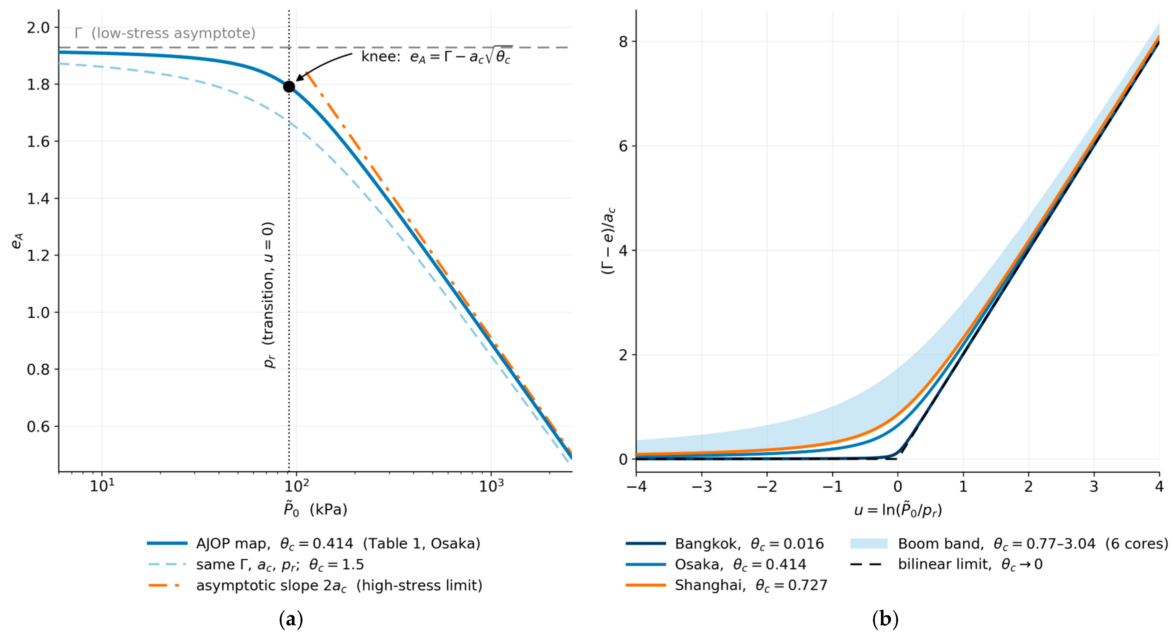
Figure 3 summarises the map. Panel (a) links $\Gamma$, $p_r$, $2a_c$, and ${\theta }_c$ to asymptote, transition, slope, and roundness. Factoring the first three in Equation (18) gives panel (b): the four calibrated curves vary only with ${\theta }_c$; changing ${\theta }_c$ selects shape, and ${\theta }_c\to 0$ recovers the bilinear limit.

3.2. Derivative Hierarchy

Here, high-order hardening means the derivatives below, not strain-gradient plasticity:

$${\lambda }_A\left(u\right)\equiv -{\displaystyle \frac{d{e}_A}{du}}=a_c\left(1+{\displaystyle \frac{u}{\sqrt{{\theta }_c+u^2}}}\right)$$

(19)

and the curvature measure is

$${\chi }_A\left(u\right)\equiv {\displaystyle \frac{d{\lambda }_A}{du}}={\displaystyle \frac{a_c\hspace{0.17em}{\theta }_c}{{\left({\theta }_c+u^2\right)}^{3/2}}}$$

(20)

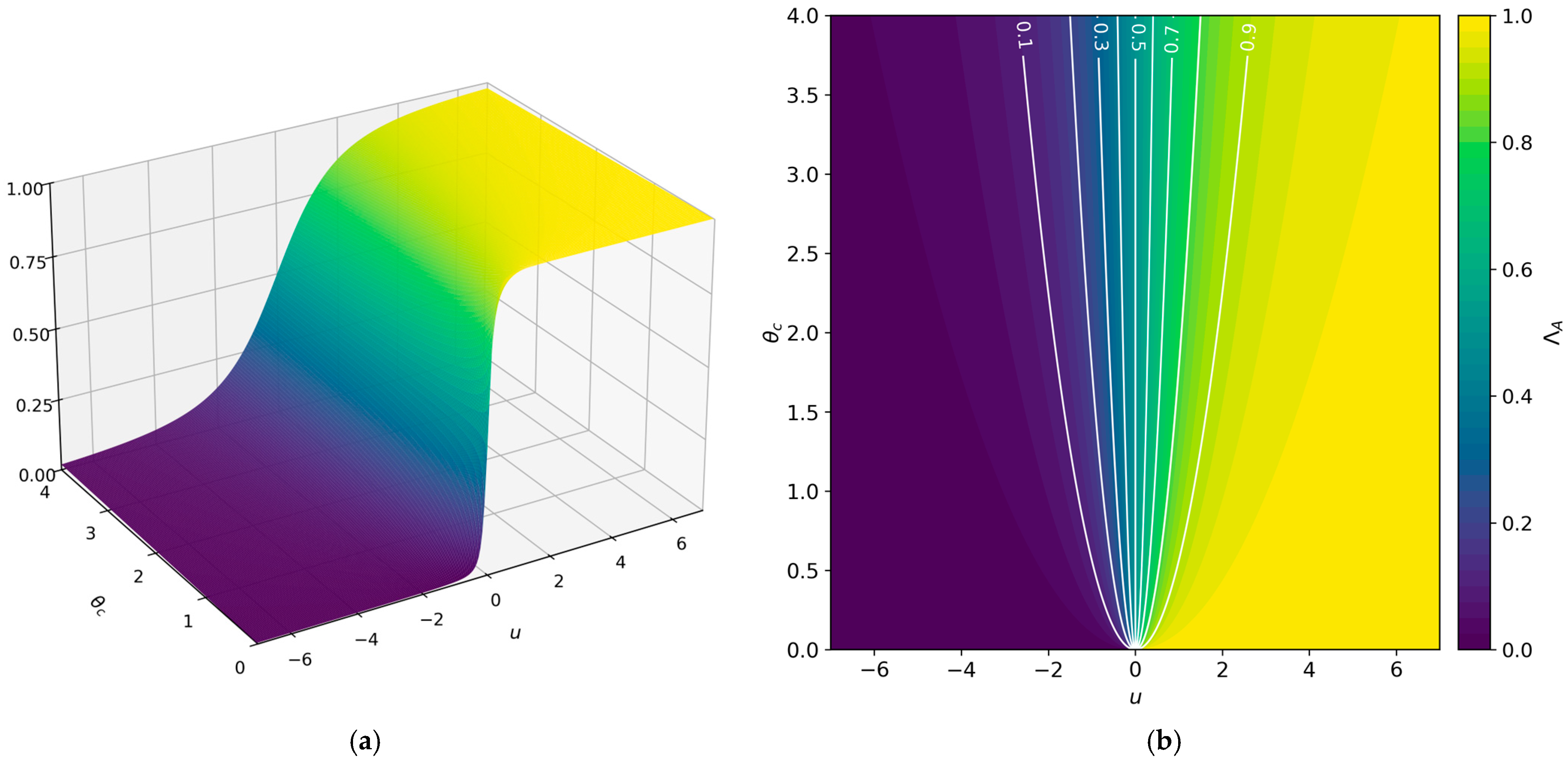
Both are smooth; ${\chi }_A>0$ makes ${\lambda }_A$ strictly increasing. Normalisation gives

$${\Lambda }_A\left(u\right)\equiv {\displaystyle \frac{{\lambda }_A\left(u\right)}{2a_c}}={\displaystyle \frac{1}{2}}\left(1+{\displaystyle \frac{u}{\sqrt{{\theta }_c+u^2}}}\right)$$

(21)

Thus ${\Lambda }_A\in \left(0,1\right)$ depends only on ${\theta }_c$; constant slope gives ${\Lambda }_A\equiv 1$ and ${\chi }_A\equiv 0$.

3.3. Limit Theorems

Theorem 1 (limit consistency).

The tangent modulus satisfies

$$\underset{u\to +\mathrm{\infty }}{\mathrm{l}\mathrm{i}\mathrm{m}}{\lambda }_A\left(u\right)=2a_c\equiv {\lambda }_{\mathrm{\infty }}, \underset{u\to -\mathrm{\infty }}{\mathrm{l}\mathrm{i}\mathrm{m}}{\lambda }_A\left(u\right)=0$$

(22)

and its maximum curvature is

$$\underset{u\in \mathbb{R}}{\mathrm{s}\mathrm{u}\mathrm{p}}{\chi }_A\left(u\right)={\chi }_A\left(0\right)={\displaystyle \frac{a_c}{\sqrt{{\theta }_c}}}$$

(23)

Proof. 

Equation (22) follows from (19); (23) follows since ${\chi }_A$ decreases with |u|. □

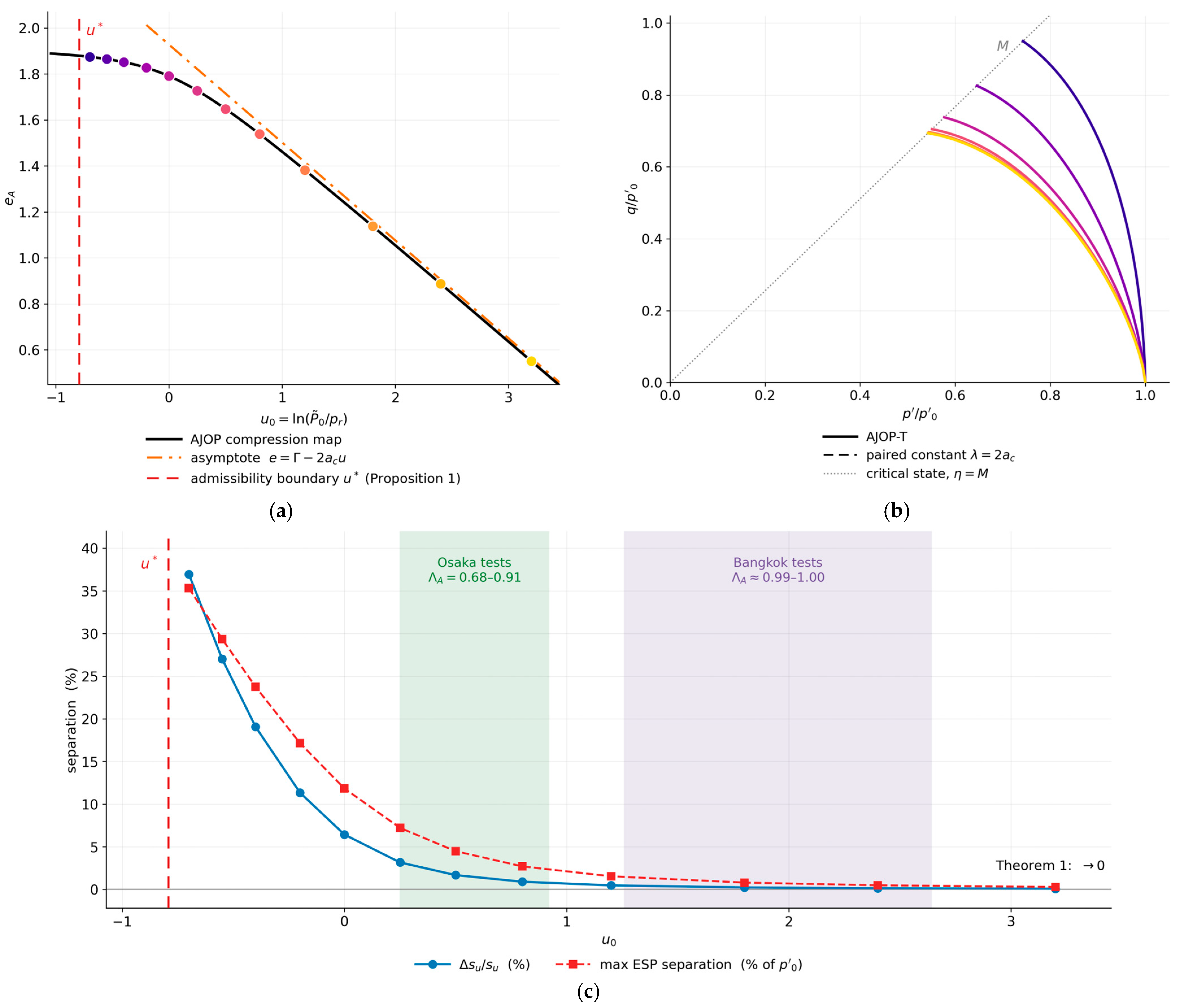
Thus, $\lambda =2a_c$ recovers the high-stress limit; ${\theta }_c$ governs sharpness and sub-transition departure. The finite-stress pair in Section 7.5 differs by only 0.27 per cent at a normalised tangent modulus of 0.882. Figure 4 visualises the dimensionless hardening and curvature surfaces.

4. AJOP-T Constitutive Embedding

4.1. Hardening Law

The AJOP-T hardening law is obtained by replacing the constant compression index in Equation (12) with the tangent modulus of Equation (19), evaluated at the current size of the bounding surface:

$$d{\tilde{P}}_0={\tilde{P}}_0\hspace{0.17em}{\displaystyle \frac{1+e_0}{{\lambda }_A\left(u\right)-\kappa }}\hspace{0.17em}d{\epsilon }_v^p$$

(24)

The swelling index $\kappa$ remains constant as the inherited phase baseline, not a cyclic swelling law; AJOP-T modifies only virgin compression. The formulation uses effective stress and assumes full saturation; at S_r = 1, w = e/G_s, so water content follows void ratio and specific gravity rather than acting as an independent hardening or geometry variable. Partial saturation is outside scope. Because $u$ is defined through ${\tilde{P}}_0$, ${\lambda }_A$ is constant along any fixed bounding surface and evolves only when the surface grows.

4.2. Admissible Hardening Domain: Closed Form

Equation (24) requires a positive denominator for the conventional hardening interpretation. The admissible hardening domain is therefore

$${\lambda }_A\left(u\right)>\kappa \iff {\Lambda }_A\left(u\right)>{\rho }_{\kappa }, {\rho }_{\kappa }={\displaystyle \frac{\kappa }{2a_c}}$$

(25)

Proposition 1 (closed-form admissibility boundary).

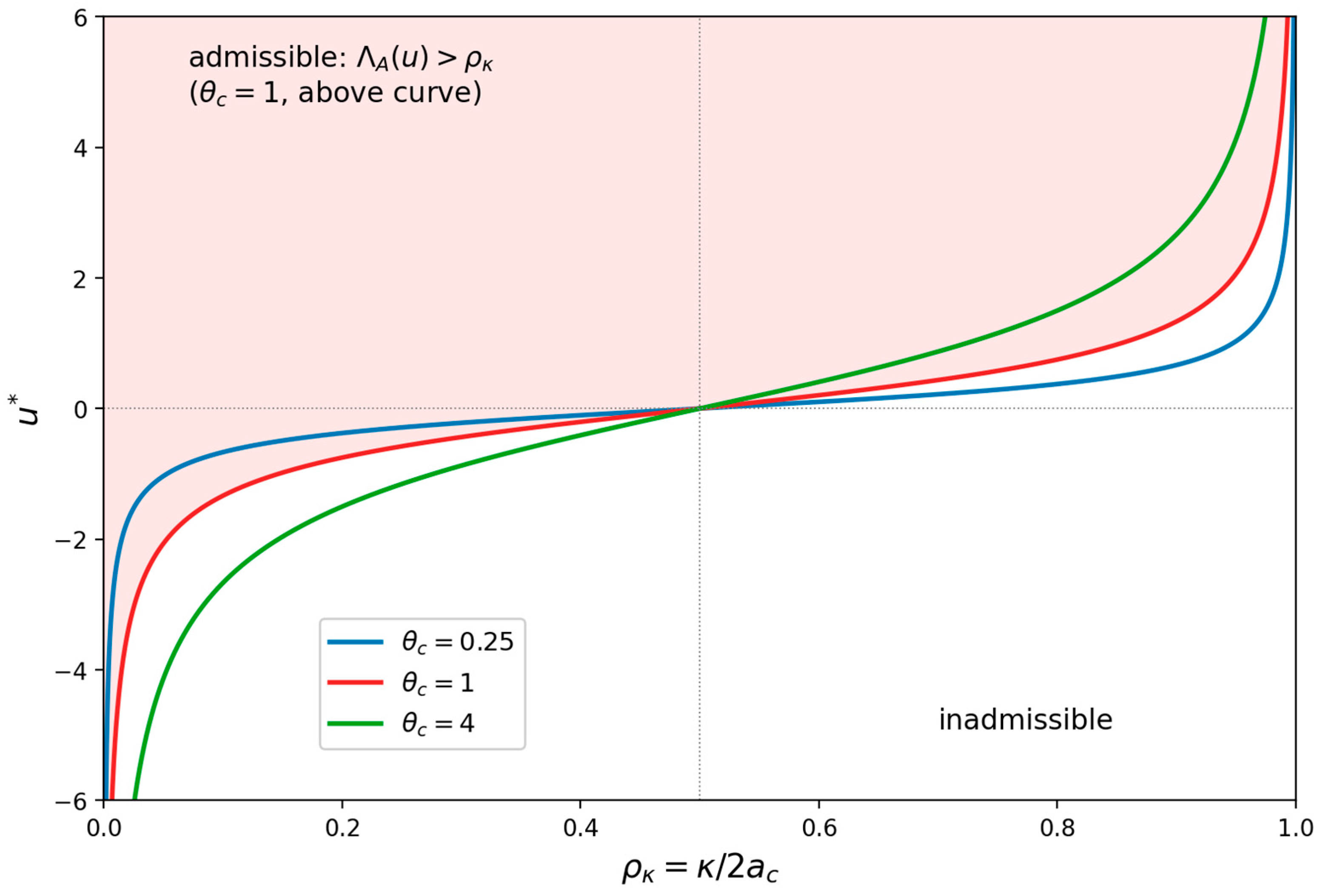
For  $0<{\rho }_{\kappa }<1$ the boundary  ${\Lambda }_A\left(u^{\ast }\right)={\rho }_{\kappa }$ has the unique solution

$$u^{\ast }=-{\displaystyle \frac{\sqrt{{\theta }_c}\hspace{0.17em}\left(1-2{\rho }_{\kappa }\right)}{2\sqrt{{\rho }_{\kappa }\left(1-{\rho }_{\kappa }\right)}}}$$

(26)

and the domain of Equation (25) is exactly  $u>u^{\ast }$.

Proof. 

Setting ${\Lambda }_A\left(u\right)={\rho }_{\kappa }$ in Equation (21) gives $u/\sqrt{{\theta }_c+u^2}=2{\rho }_{\kappa }-1\in \left(-1,1\right)$. Writing $t=u/\sqrt{{\theta }_c}$, the relation $t/\sqrt{1+t^2}=2{\rho }_{\kappa }-1$ inverts uniquely to $t=\left(2{\rho }_{\kappa }-1\right)/\sqrt{1-{\left(2{\rho }_{\kappa }-1\right)}^2}$, and $1-{\left(2{\rho }_{\kappa }-1\right)}^2=4{\rho }_{\kappa }\left(1-{\rho }_{\kappa }\right)$, giving Equation (26). Uniqueness and the form of the domain follow from the strict monotonicity of ${\Lambda }_A$. □

For the practically relevant case ${\rho }_{\kappa }<1/2$ (swelling slope below the asymptotic half-slope), $u^{\ast }<0$: the singularity of the hardening denominator lies on the strongly curved low-stress branch, at a distance from the transition that scales with $\sqrt{{\theta }_c}$. The singularity is not removed in AJOP-T; it is mapped. Proposition 1 turns the admissibility question from a numerical observation into an explicit inequality that can be checked before any integration is attempted, and Figure 5 renders the boundary in the $\left(\rho \kappa {,}_u\right)$ plane. A stress-dependent swelling law would be required to remove the singularity by construction; its calibration and cyclic consequences are deliberately deferred to a separate model phase.

Proposition 1 has a practical reading, and it is the reason the boundary is given in closed form rather than located numerically. For every calibration within the domain of Proposition 1, there is a stress below which this hardening law stops meaning what it is intended to mean. That stress follows from the compression parameters alone, so it can be computed before an analysis begins and compared against the shallowest element in a mesh. A check costing one line of code replaces a division by a vanishing quantity that would otherwise appear in the middle of a stress-point iteration, where it is expensive to diagnose.

4.3. Plastic Modulus, Consistency and Elasto-Plastic Tangent

This subsection is where the hardening law becomes something a finite element code can call. Three objects are required at a Gauss point: a plastic modulus, a consistency condition that fixes the plastic multiplier, and a tangent matrix that relates a strain increment to a stress increment. All three are assembled below, and all three are in closed form. The reader interested only in implementation may take Equation (31) and its hardening modulus as the output of this section.

The plastic modulus of Equation (13) becomes, with the same $M_k$ interpolation of Equations (14)–(16),

$$K_p^A={\displaystyle \frac{1+e_0}{{\lambda }_A\left(u\right)-\kappa }}\left(M_k-\tilde{\eta }\right){\displaystyle \frac{\partial g}{\partial \tilde{Q}}}$$

(27)

For implementation in strain-driven form, let ${\mathbf{D}}^e$ be the elastic stiffness, $\mathbf{n}=\partial F/\partial \tilde{\mathsf{\sigma }}$ the outward normal evaluated at the image point through Equations (7) and (8), and $\mathbf{m}$ the flow direction of Equation (10) with the $M_k$ substitution of the base model. The elastic law is isotropic and pressure-dependent, with bulk modulus $K=(1+e_0)\stackrel{\sim }{p}\prime /\kappa$ and shear modulus $G=3K(1-2\nu )/\left[2\right(1+\nu \left)\right]$ at constant Poisson ratio $\nu$; every simulation in this paper uses $\nu =0.3$. The stress increment and plastic multiplier are

$$d\tilde{\mathsf{\sigma }}={\mathbf{D}}^e\left(d\mathsf{\epsilon }-d\Lambda \hspace{0.17em}\mathbf{m}\right)$$

(28)

$$d\Lambda ={\displaystyle \frac{{\mathbf{n}}^{\mathsf{T}}{\mathbf{D}}^e\hspace{0.17em}d\mathsf{\epsilon }}{{\mathbf{n}}^{\mathsf{T}}{\mathbf{D}}^e\mathbf{m}+H_A}}$$

(29)

where the AJOP hardening modulus follows from the consistency condition $dF=0$ with Equations (9) and (24):

$$H_A=-{\displaystyle \frac{\partial F}{\partial {\tilde{P}}_0}}\hspace{0.33em}{\displaystyle \frac{\partial {\tilde{P}}_0}{\partial {\epsilon }_v^p}}\hspace{0.33em}{m}_v={\displaystyle \frac{\Omega \left(1+e_0\right)\left(M_k-\tilde{\eta }\right)}{\left({\lambda }_A\left(u\right)-\kappa \right)M\tilde{P}}}$$

(30)

The consistency condition alone delivers Equation (30) with $M$ in place of $M_k$, since it is enforced on the bounding surface where $R$ = 1; the virtual peak stress ratio $M_k$ replaces $M$ in the numerator through the bounding surface interpolation of [12], exactly as in Equation (27), while the factor $M$ in the denominator originates in the flow direction of Equation (10) and is not interpolated.

Lemma 1 (cancellation of the explicit size factor).

$H_A$ contains no standalone multiplicative factor  ${\tilde{P}}_0$: the factor  ${\tilde{P}}_0$ from  $\partial {\tilde{P}}_0/\partial {\epsilon }_v^p$ cancels  ${\tilde{P}}_0^{-1}$ in  $\partial F/\partial {\tilde{P}}_0$. It nevertheless depends on stress scale through the image mean stress P in Equation (30), and on size and history through  $u$ in  ${\lambda }_A\left(u\right)$, with  $R$ also entering through  $M_k$. The cancellation therefore does not make the modulus size-independent.

The corresponding elasto-plastic tangent is

$${\mathbf{D}}^{ep}={\mathbf{D}}^e-{\displaystyle \frac{{\mathbf{D}}^e\hspace{0.17em}\mathbf{m}\hspace{0.17em}{\mathbf{n}}^{\mathsf{T}}{\mathbf{D}}^e}{{\mathbf{n}}^{\mathsf{T}}{\mathbf{D}}^e\mathbf{m}+H_A}}$$

(31)

Equation (31) is the continuum elasto-plastic tangent in transformed stress space; AJOP enters only through $H_A$. The normal $\mathbf{n}$, flow direction $\mathbf{m}$, mapping rule and transformed stress remain those of the base model [10]. It is not a discretisation-consistent algorithmic tangent for a particular integration scheme; deriving that tangent remains future work.

4.4. Sensitivity of the Hardening Modulus

Because $H_A$ depends on ${\lambda }_A$, and ${\lambda }_A$ depends on the hardening coordinate $u$, the hardening modulus has a stress-domain sensitivity absent from constant-slope hardening. Differentiating Equation (30) at fixed stress state and spacing ratio gives

$${\displaystyle \frac{\partial H_A}{\partial u}}=-H_A\hspace{0.17em}{\displaystyle \frac{{\chi }_A\left(u\right)}{{\lambda }_A\left(u\right)-\kappa }}$$

(32)

Equation (32) is one of the reasons the term high-order hardening is appropriate: the second derivative ${\chi }_A$ controls the sensitivity of the plastic modulus itself, not merely the shape of a compression curve. It is also the ingredient required by the Jacobian of an implicit (backward Euler) stress-integration scheme of the Cam-clay return-mapping family [34], in which the derivative of the hardening modulus with respect to the state variables enters the consistent tangent; Equation (32) supplies that derivative in closed form. Substepping schemes with automatic error control [35] are the standard explicit alternative to such implicit integrators.

5. Structural Theorems

Four results are proved in this section, and each answers a different question. Does a calibration made on compression data survive the passage to general stress space? Does the new formulation still contain the settlement equation it was built from? Where does the critical state line sit once the compression curve is allowed to bend? And is the undrained strength ratio that follows bounded, or can it run away at low stress? The proofs are short, and the algebra is elementary. The consequences are not, and each proof is followed by a statement of what it means for an analysis.

5.1. Invariance of the Hardening Hierarchy Under the SMP Transformed Stress

Remark 3 (invariance of the hardening hierarchy).

The transformed stress mapping of Equation (1) leaves the mean stress unchanged,

$$\tilde{p}={\displaystyle \frac{1}{3}}{\tilde{\sigma }}_{ii}=p+{\displaystyle \frac{1}{3}}{\displaystyle \frac{q_{\mathrm{S}\mathrm{M}\mathrm{P}}}{q_c}}\hspace{0.17em}{s}_{ii}=p$$

(33)

since $s_{ii}=0$. Consequently, the volumetric hardening structure of AJOP-T—the coordinate $u$, the hierarchy $e_A,{\lambda }_A,{\chi }_A$, the admissibility domain of Proposition 1 and the hardening law of Equation (24)—is invariant under the SMP mapping. The transformed stress modifies only the deviatoric direction of the stress point; the compression-derived hierarchy and the yield-geometry machinery act on orthogonal parts of the formulation.

This orthogonality is a structural property, not a coincidence: the SMP mapping of [10] is constructed as a deviatoric rescaling at fixed mean stress, and the AJOP hierarchy is a function of the volumetric history alone. This result guarantees that calibration of $\left(\Gamma ,a_c,{\theta }_c,p_r\right)$ from one-dimensional or isotropic compression data remains unchanged when the model is exercised in general stress space.

5.2. Exact Recovery of the Settlement Equation

Theorem 2 (recovery of the refined consolidation settlement equation).

Consider isotropic loading of a normally consolidated state:  $R=1$,  $\tilde{\eta }=0$, and the stress point remains on the bounding surface with  $\tilde{p}={\tilde{P}}_0$. Then the total void-ratio increment predicted by AJOP-T satisfies

$$de=-{\lambda }_A\left(u\right)\hspace{0.17em}du$$

(34)

and integrates exactly to $e\left(u\right)=e_A\left(u\right)+C$ with $C=0$ when the integration constant is fixed by the asymptote  $\Gamma$. In particular, the void-ratio change between two preconsolidation states $u_1$ and $u_2$ is

$$\Delta e=e_A\left(u_1\right)-e_A\left(u_2\right)$$

(35)

which is the refined consolidation settlement equation of Phonchamni et al. [24] expressed in natural-logarithm variables (Remark 2). AJOP-T therefore collapses to the settlement formulation of [24] under isotropic normally consolidated loading, with no residual terms.

Proof. 

On the isotropic NC path, the elastic and plastic void-ratio increments are  $d{e}^e=-\kappa \hspace{0.17em}du$ and, from Equation (24) with $d{\epsilon }_v^p=-d{e}^p/\left(1+e_0\right)$ and $d{\tilde{P}}_0/{\tilde{P}}_0=du$, $d{e}^p=-\left({\lambda }_A\left(u\right)-\kappa \right)\hspace{0.17em}du$. Summing gives Equation (34); integrating Equation (19) recovers Equation (18) up to a constant, and Equation (35) follows. □

Theorem 2 serves two purposes. Scientifically, it establishes that AJOP-T is the constitutive completion of the settlement-equation formulation of [24]: the same four compression parameters govern both, and no re-fitting is needed at the oedometric level. Computationally, it is the first invariant check of the numerical implementation: an isotropic compression simulation must reproduce $e_A\left(u\right)$ to machine precision, and any deviation indicates an integration or wiring error rather than a modelling discrepancy.

For an engineer, Theorem 2 is a compatibility statement for the isotropic NC path. With the same soil parameters and the same isotropic NC loading, the published one-dimensional formula and the full constitutive model give the same settlement. No recalibration of the compression map is required. A disagreement under that restriction therefore indicates an implementation or loading-path mismatch; outside it, the stress path and boundary conditions can produce different settlements.

5.3. Emergence of the Critical State Line

The position of the critical state line (CSL) in the compression plane is not a free modelling choice in AJOP-T: it is fixed by the inherited bounding surface geometry. Setting $\tilde{\eta }=M$ in Equation (4) gives $\Omega \mathrm{l}\mathrm{n}\left({\tilde{P}}_{cs}/{\tilde{P}}_0\right)=-1$, so the critical-state mean stress on any bounding surface stands at the fixed fraction

$${\tilde{P}}_{cs}={\tilde{P}}_0\hspace{0.17em}{e}^{-1/\Omega }$$

(36)

of the surface size, for every member of the family.

Remark 4 (volumetric convention).

Equation (24) and Theorem 2 carry the fixed factor $(1+e_0)$ of the initial state rather than the evolving $(1+e)$, matching the convention of the refined consolidation settlement equation itself; this is what makes the recovery of Theorem 2 exact by construction rather than asymptotic. Over wide stress ranges, the two conventions differ. All computations reported here use the fixed initial-state factor of Equation (24).

Proposition 2 (CSL emergence).

With the hardening law of Equation (24) and constant swelling index $\kappa$, the locus of critical states in the $\left(e,ln\tilde{p}\right)$ plane is

$$e_{cs}\left(\tilde{p}\right)=e_A \left(\mathrm{l}\mathrm{n} \left({\displaystyle \frac{\tilde{p}}{p_r}}\right)+{\displaystyle \frac{1}{\Omega }}\right)+{\displaystyle \frac{\kappa }{\Omega }}$$

(37)

that is, the AJOP normal compression curve translated by $1/\Omega$ along the $\mathrm{l}\mathrm{n}\tilde{\mathrm{p}}$ axis and by  $\kappa /\Omega$ in void ratio. The CSL therefore curves with the normal compression line as a consequence of the formulation, not as an assumption.

Proof. 

A normally consolidated state on the bounding surface of size ${\tilde{P}}_0$ carries $e=e_A\left(u\right)$ with $u=\mathrm{l}\mathrm{n}\left({\tilde{P}}_0/p_r\right)$ by Theorem 2. Reaching the critical state on that surface changes the mean stress from  ${\tilde{P}}_0$ to ${\tilde{P}}_{cs}={\tilde{P}}_0{e}^{-1/\Omega }$ of Equation (36); the associated elastic void-ratio change is $+\kappa \mathrm{l}\mathrm{n}\left({\tilde{P}}_0/{\tilde{P}}_{cs}\right)=\kappa /\Omega$, while the plastic component is fixed by the surface size. Eliminating ${\tilde{P}}_0={\tilde{P}}_{cs}\hspace{0.17em}{e}^{1/\Omega }$ gives Equation (37). □

The vertical spacing between the normal compression curve and the CSL at the same mean stress follows directly:

$$\Delta e\left(u\right)=e_A\left(u\right)-e_A \left(u+{\displaystyle \frac{1}{\Omega }}\right)-{\displaystyle \frac{\kappa }{\Omega }}={\displaystyle \frac{{\lambda }_A\left(\bar{u}\right)-\kappa }{\Omega }}, \bar{u}\in \left(u,u+{\displaystyle \frac{1}{\Omega }}\right)$$

(38)

by the mean value theorem. Equation (38) must not be conflated with the local admissibility condition. For every admissible state, the strict increase of ${\lambda }_A$ makes the average slope over the finite logarithmic interval exceed κ, so the NCL–CSL spacing remains positive. It does not vanish where ${\lambda }_A=\kappa$; as the hardening coordinate approaches $u^{\ast }$ from above, the spacing tends to 0.0355 in void ratio at p′* = 41.5 kPa. The boundary is therefore the local hardening-denominator limit, not closure of NCL–CSL spacing. Proposition 2 still supplies a machine-precision implementation check: simulated critical states must fall on Equation (37).

Equation (38) shows that the NCL–CSL gap is governed by the average compression tangent over a finite logarithmic stress interval. The gap narrows on the low-stress branch but does not close within the admissible domain. A straight compression line is the constant-slope special case, for which the same gap is constant by construction.

5.4. Semi-Analytical Undrained Strength Ratio

Proposition 2 makes the undrained strength of a normally consolidated state semi-analytical. Consider undrained triaxial compression from an isotropic NC state at mean stress ${{\tilde{p}}_0}^{\prime }={\tilde{P}}_0$, hardening coordinate $u_0$, and void ratio $e_A\left(u_0\right)$. At constant volume, the state reaches the critical state at the mean stress ${\tilde{p}}_{cs}$ whose critical-state void ratio equals $e_A\left(u_0\right)$; by Equation (37) the coordinate $u_{cs}=ln\left({\tilde{p}}_{cs}/p_r\right)$ solves the scalar implicit equation

$$e_A \left(u_{cs}+{\displaystyle \frac{1}{\Omega }}\right)=e_A\left(u_0\right)-{\displaystyle \frac{\kappa }{\Omega }}$$

(39)

which has a unique root by the strict monotonicity of $e_A$. The undrained strength in triaxial compression (where the SMP mapping leaves the stress point unchanged) is $s_u=q_{cs}/2=M{\tilde{p}}_{cs}/2$, so the strength ratio is

$${\displaystyle \frac{s_u}{{\tilde{p}}_0\prime }}={\displaystyle \frac{M}{2}}\hspace{0.17em}{e}^{\hspace{0.17em}{u}_{cs}-u_0}$$

(40)

Corollary 1 (high-stress limit).

In the log-linear regime  ${\lambda }_A\to 2a_c$, Equations (39) and (40) reduce to

$${\displaystyle \frac{s_u}{{{\tilde{p}}_0}^{\prime }}}\hspace{0.33em}\to \hspace{0.33em}{\displaystyle \frac{M}{2}}\hspace{0.17em}\mathrm{e}\mathrm{x}\mathrm{p} \left(-{\displaystyle \frac{1-{\rho }_{\kappa }}{\Omega }}\right)$$

(41)

which is the classical stress-level-independent strength ratio of critical state soil mechanics [36] with plastic volumetric ratio $1-{\rho }_{\kappa }=1-\kappa /{\lambda }_{\mathrm{\infty }}$ and spacing constant $e^{1/\Omega }$.

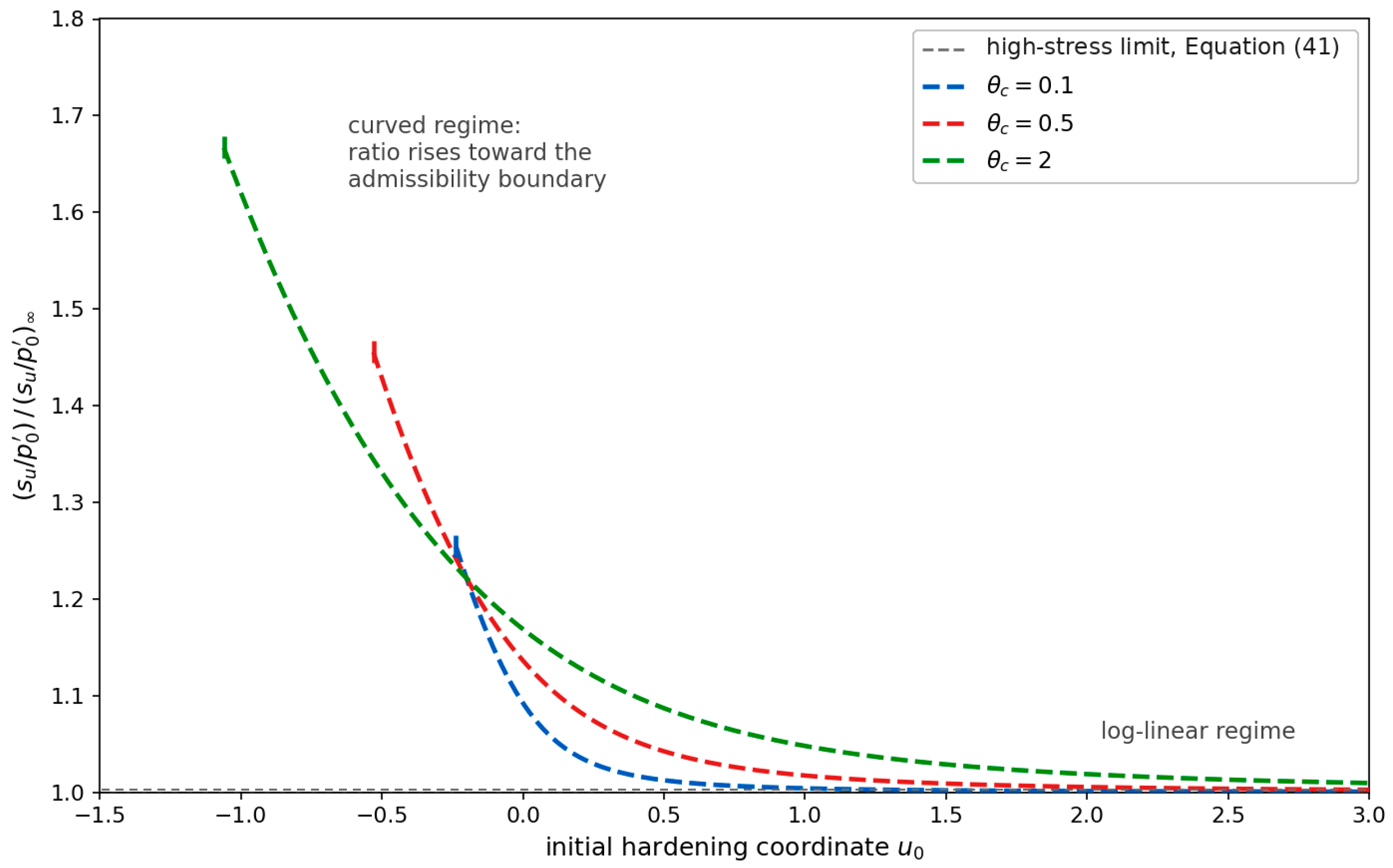
Away from that limit, the ratio is stress-level dependent: as $u_0$ decreases into the curved regime, the NCL–CSL spacing of Equation (38) shrinks, ${\tilde{p}}_{cs}$ approaches ${{\tilde{p}}_0}^{\prime }$, and the ratio rises above the asymptotic value—monotonically, toward a finite limit that Corollary 2 bounds by $M/2$ at the admissibility boundary. This drift is a distinctive, testable prediction of AJOP-T—a direct constitutive counterpart of the low-stress compression curvature that motivates the AJOP law—and Figure 6 quantifies it in dimensionless form. Low-stress critical-state data for reconstituted clays are scarce, so this prediction is stated as a falsifiable feature rather than a validated one. The asymptotic ratio itself is the quantity organised by normalised-strength practice—the SHANSEP procedure of Ladd and Foott [37] and the in situ strength interpretation of Wroth [38]—so the predicted low-stress drift is expressed directly in the normalisation used to report undrained strength.

Corollary 2 (boundedness of the undrained strength ratio).

On the admissible domain of Proposition 1, every normally consolidated initial state satisfies $s_u/{{\stackrel{\sim }{p}}^{\prime }}_0\le M/2$, and the ratio approaches a finite limit as  $u_0$ approaches the boundary of Proposition 1.

Proof. 

Admissibility gives ${\lambda }_A\left(u\right)\ge \kappa$ for all $u\ge u_0$, so $e_A\left(u_0\right)-e_A(u_0+1/\Omega )\ge \kappa /\Omega$. Combining this with the critical-state locus of Proposition 2 gives $u_{cs}\le u_0$, hence by Equations (39) and (40) $s_u/{\stackrel{\sim }{p}\prime }_0=(M/2)exp(u_{cs}-u_0)\le M/2$. As $u_0$ approaches the boundary, the spacing relation determines $u_{cs}$ continuously up to it—the root is unique by the strict monotonicity of $e_A$—so the ratio extends continuously to a limit strictly below $M/2$, because ${\lambda }_A>\kappa$ on the interior of the spacing interval. □

Corollary 2 answers the question that should be asked of any curved compression law. If the undrained strength ratio rises as the stress level falls, does it rise without limit? It does not: throughout the admissible domain the ratio stays strictly below half the critical-state stress ratio and approaches a finite boundary limit that is itself below M/2. The prediction is therefore finite and falsifiable, which is what makes it worth testing against low-stress data rather than merely asserting.

6. Response Space and Data-Anchored Evaluation Program

This section defines the numerical illustrations of the formulation. Figure 4, Figure 5, Figure 6, Figure 7 and Figure 8 expose the response space generated by the high-order hardening law and are not validation against a particular clay. Figure 9 provides paired constant-slope/AJOP responses on identical parameters. Figure 10 anchors the AJOP compression map to laboratory compression data, and Figure 11, Figure 12 and Figure 13 extend the data-anchored evaluation to three further natural clays. The compression and triaxial datasets used for parameter estimation are reported as fitted comparisons; the Eastern Osaka extension path is the only held-out stress-path check.

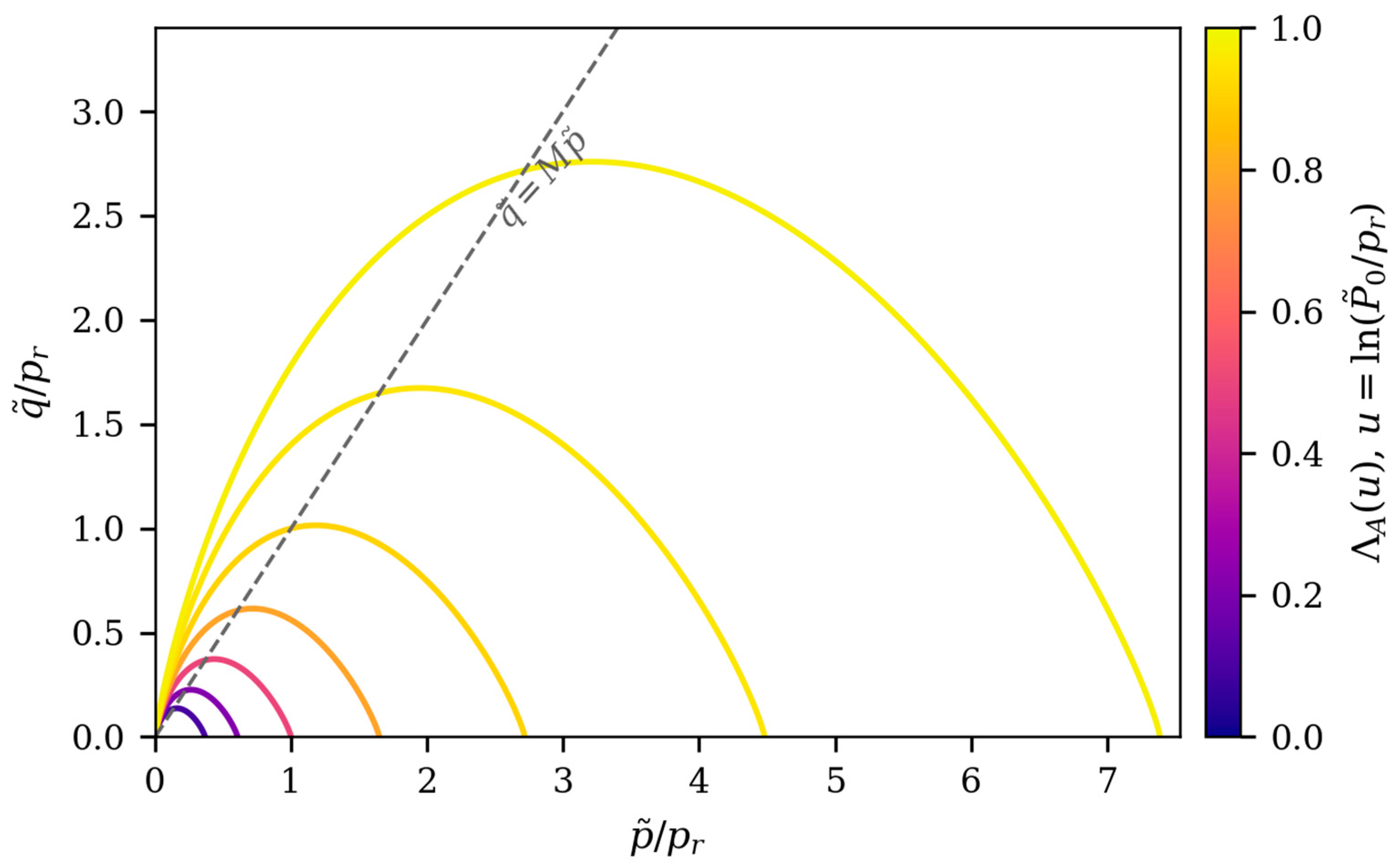
6.1. Teardrop Surface Family Coloured by Hardening State

The teardrop geometry of Equation (4) is independent of AJOP, but the speed at which the bounding surface family is traversed depends on ${\lambda }_A$. Because $u$ is defined through ${\tilde{P}}_0$, the value ${\Lambda }_A$ is a single number on each member of the nested surface family. The correct visualisation is therefore a family plot: nested teardrop surfaces at increasing ${\tilde{P}}_0$, each coloured by its own ${\Lambda }_A\left(u\right)$, so that the colour gradient across the family displays the hardening transition while each individual surface remains a single hardening state.

6.2. Curvature-Induced Hardening Trajectories

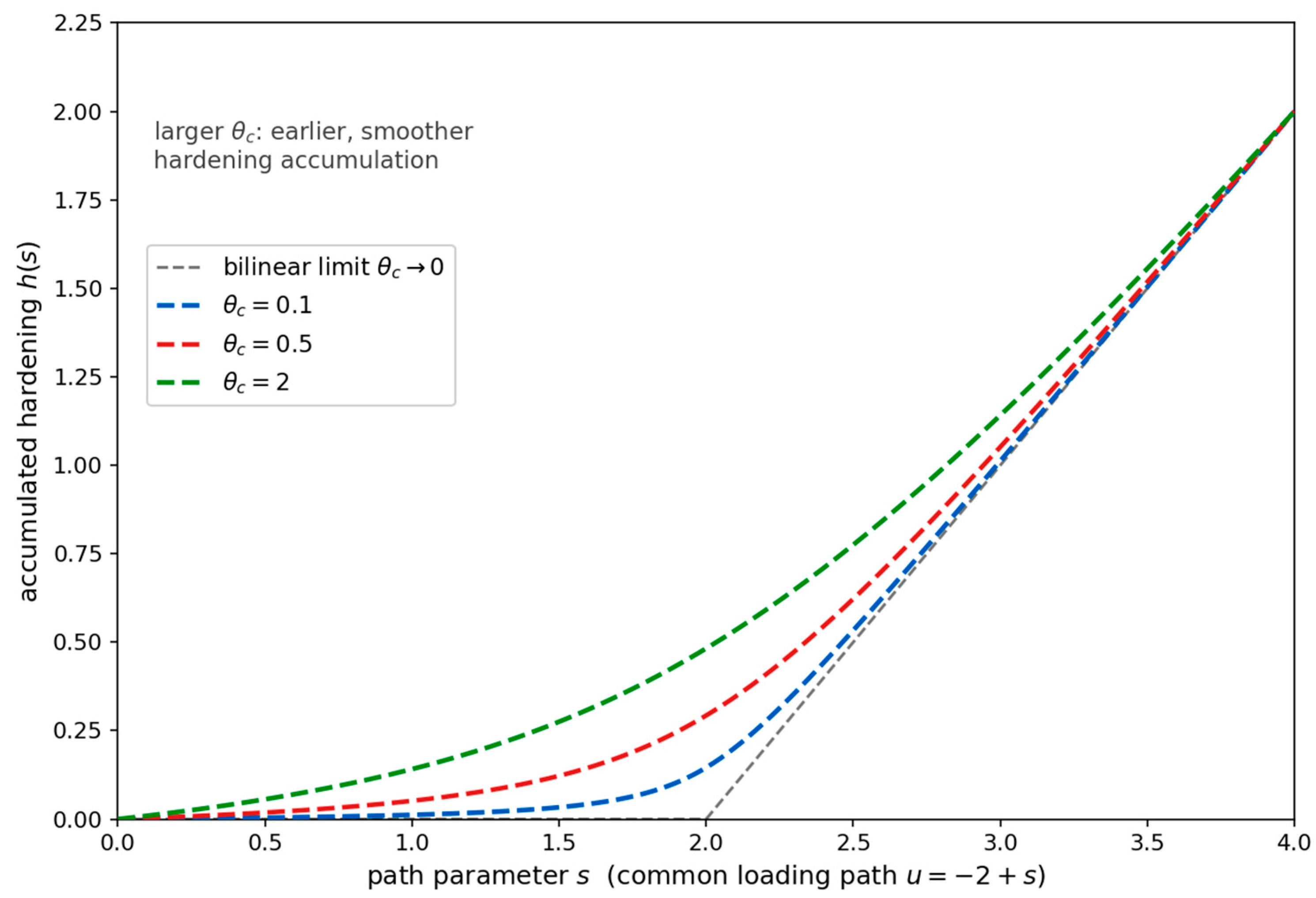
For a path parameter $s$ representing accumulated plastic loading, the normalised accumulated hardening is written as the diagnostic quantity

$$\widehat{h}\left(s\right)={\int }_0^s{\Lambda }_A \left(u\left(\tau \right)\right)d\tau$$

(42)

Equation (42) is not a new constitutive assumption; it is a diagnostic used to compare how different roundness values ${\theta }_c$ alter accumulated hardening along the same path before convergence to the linear asymptote.

Figure 9 assembles the paired-response map that the preceding subsections imply. Eight normally consolidated initial states are placed on the AJOP compression curve, from near the admissibility boundary of Proposition 1 to deep on the high-stress asymptote, and each state is sheared undrained twice on identical parameters: once with ${\lambda }_A\left(u\right)$ and once with the paired constant slope $\lambda =2a_c$. On the asymptote, the two responses coincide, which is Theorem 1 read in response space; at the transition, the pair separates by a few per cent; near the boundary, the plotted path separation is 35.4% of ${p\prime }_0$ and the strength separation is 37.0%. The map also locates the laboratory programs of Section 6.3: the Eastern Osaka tests sit at ${\Lambda }_A$ = 0.68–0.91 and the Bangkok tests at ${\Lambda }_A$ ≈ 0.99–1.00, so their paired curves are expected to nearly coincide—the hierarchy is exercised by these data through the compression map and the emergent critical state, not through visible path separation.

Read as a profile, Figure 9a answers the engineer’s first screening question: where might the change matter? Its horizontal axis is $u_0=\mathrm{l}\mathrm{n}({\tilde{P}}_0/p_r)$, equal to $\mathrm{l}\mathrm{n}({p^{\prime }}_0/p_r)$ for NC states and can be mapped to depth. Below the admissibility boundary, the formulation is undefined; for the stated effective unit weight of 8 kN/m³ and K₀ = 0.55, the 41.5 kPa boundary maps to about 7 m. Above the transition, the two hardening laws coincide to the printed digits. Between them lies the band worth screening: for Eastern Osaka, the paired undrained-strength difference is 24 per cent at 10 m, 8 per cent at 15 m, 3.6 per cent at 20 m and 1.3 per cent at 30 m under that profile assumption.

The width of that band is material-specific. The roundness parameter is 0.414 for Eastern Osaka and 0.016 for weathered Bangkok; the latter produces a sharp transition rather than a broad curved band. Its normalised tangent modulus rises from 0.32 to 0.97 between 5 m and 7.5 m on the same assumed profile, so the paired difference is below 0.3 per cent beneath the uppermost few metres. This explains why the Bangkok simulations of Section 6.3 reproduce their constant-slope twins to three significant digits.

Two practical consequences follow. First, for surface loading the stress-transition band can overlap the shallow zone contributing strongly to settlement, so curvature may be amplified rather than averaged out. Second, relevance can be screened before a mesh is built: fit the compression curve, evaluate Proposition 1 and the normalised tangent modulus over the stress range of interest, then decide whether a curved hardening law warrants analysis.

6.3. Data-Anchored Calibration and Model–Data Checks Across Four Natural Clays

The evidence hierarchy is stated before the comparisons are interpreted.

Table 1. Dataset, test program, data use and evidential role; complete specimen and test metadata are given in Table A2.

Dataset/Source	Test and Stress Range	Data Used	Evidential Role
Boom Clay [39]	Drained high-pressure Oedometer; σ′v = 0.125–32 MPa	6 curves × 9 points (Nfit = 54)	Compression-map calibration; external slope and stress-scale consistency checks
Eastern Osaka KSS5-1 [33]	Drained isotropic consolidation; yield pressure 93.1 kPa	Nfit = 9	Compression-map calibration; external yield check
Eastern Osaka TSK [33]	Isotropic consolidation and undrained triaxial compression; p′0 = 19.6–235.2 kPa	5 paths	Ψ and Ω calibration; fitted comparison
Eastern Osaka TS6-2 [33]	Isotropic consolidation and undrained triaxial extension; p′0 = 117.6 kPa	1 path	Held-out prediction
Shanghai layer 4 [40]	Drained one-dimensional Oedometer; approximately 12–2200 kPa	Nfit = 15	Compression-map calibration; external yield check
Weathered Bangkok [41]	Drained isotropic consolidation	Digitised fitted curve; Nfit not retained (NA-D)	Compression-map calibration
Weathered Bangkok [41]	Isotropic consolidation and nominally normally consolidated undrained triaxial compression; p′0 = 103–414 kPa	4 paths; 25 resampled levels per path	Ψ and Ω calibration; fitted comparison

summarises each dataset, test program, data count and evidential role; complete specimen properties, test conditions, analysis-start states and quantitative comparisons are retained in Table A2. The four AJOP compression-map parameters were estimated separately from the corresponding compression curves. The Eastern Osaka TSK compression paths and weathered Bangkok undrained paths were then used to calibrate Ψ and Ω and are fitted comparisons, whereas the Eastern Osaka TS6-2 extension path was excluded from calibration and is a held-out prediction. Published compression indices and yield pressures serve only as external scalar checks.

Table 2. Data-anchored AJOP compression-map calibrations and external scalar checks for four natural clays.

Clay (Data Type)	$\mathit{\Gamma }$	${\mathit{a}}_{\mathit{c}}$	${\mathit{\theta }}_{\mathit{c}}$	${\mathit{p}}_{\mathit{r}}$	RMS(e) × 103	Published $\mathit{\lambda }$/Independent Check
Boom Clay, 6 cores [39] (HP Oedometer)	0.643–0.840	0.073–0.119	0.77–3.04	1.55–6.27 MPa	3.7–7.7	per-core ${\lambda }_A$ in Figure 10
Weathered Bangkok [41] (isotropic + CIU)	3.465	0.369	0.016	29.4 kPa	23.3	$\lambda$ = 0.51 (basis ambiguous; curve gives $C_c$ ≈ 1.6–1.9); $p_{yield}$ ≈ 40 kPa
Eastern Osaka [33] (isotropic)	1.928	0.213	0.414	91.6 kPa	4.5	$\lambda$ = 0.355 (ln), slope check 0.374; $P_c$ = 93.1 kPa (−1.6%)
Shanghai layer 4 [40] (Oedometer, undist.)	1.155	0.089	0.727	91.2 kPa	4.3	intrinsic $\lambda$ = 0.140 (ln); $p_c$ ≈ 90–100 kPa

Notes: Compression-map parameters (Γ, a_c, θ_c, p_r) are free least-squares fits to first-loading curves; Boom Clay per-core values are in Figure 10. For Bangkok, M = 0.90 and κ = 0.12 are from [41] (natural-log basis assumed), Ψ = 1.4 and Ω = 1.45 are fitted to the stress paths, and initial void ratios come from the compression map. For Osaka, M = 1.279 and κ = 0.0477 (published); Ψ and Ω are shared. Both use ν = 0.3.

reports the fitted AJOP parameters and error measures.

All experimental observations are secondary data digitised from the cited publications. Table A2 records metadata transcribed from the primary sources where available. Values marked D were derived from source-reported stresses, digitised ordinates or the fitted compression map; unreported specimen quantities were not imputed. NA-D denotes information unavailable in the digitised analysis record. N_fit counts ordinates used for parameter estimation; resampled objective-grid ordinates are not independent measurements. For the Bangkok compression curve, the fitted ordinates and RMS are retained, but their count is not, so N_fit is reported as NA-D.

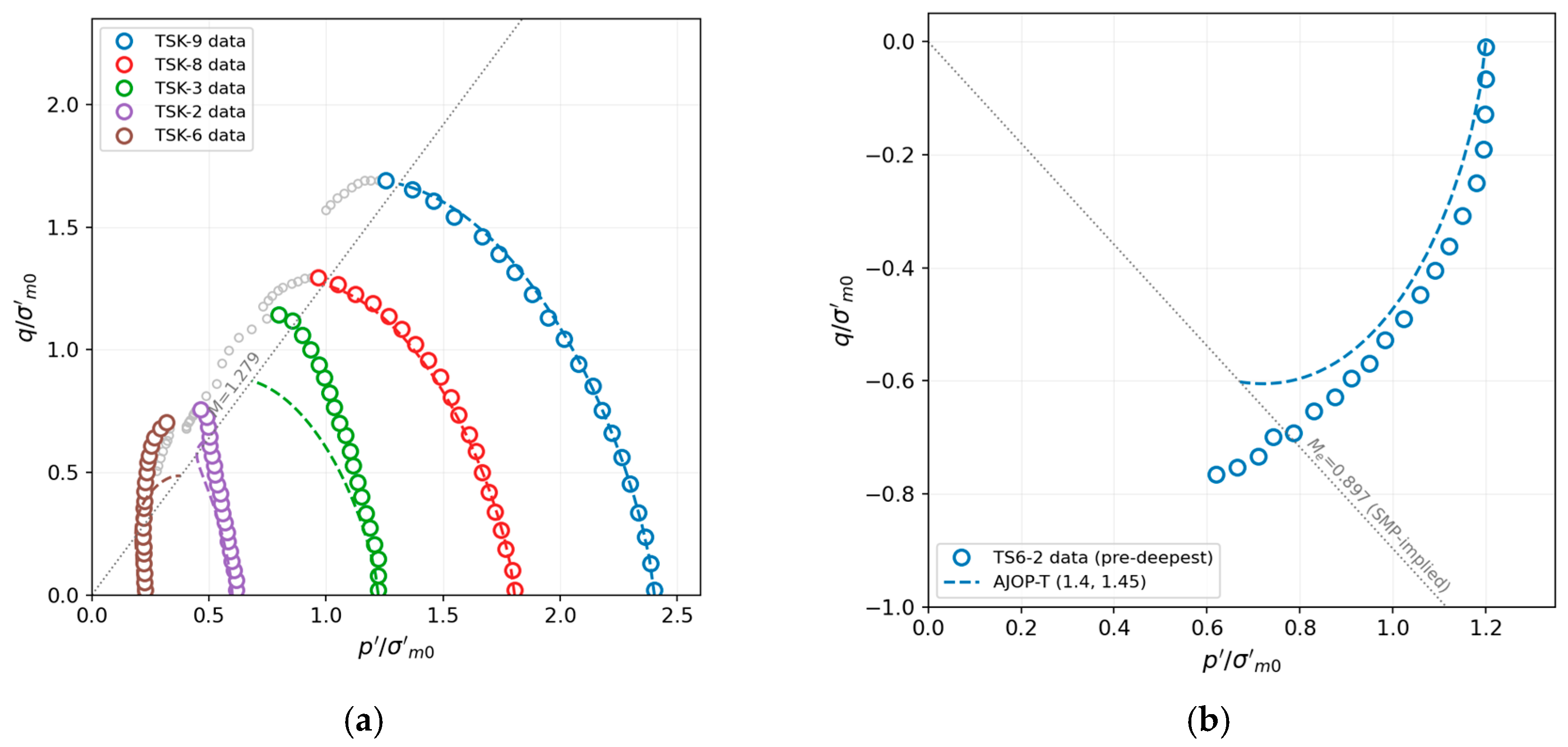
This accounting changes the interpretation but not the numerical comparisons. Figure 10 and Figure 11 are compression-map calibrations. Figure 12a and Figure 13 are fitted comparisons, because the plotted compression paths contributed to the calibration of Ψ and Ω. Figure 12b is the only held-out stress-path check in the present dataset. Accordingly, validation is reserved below for genuinely held-out information, and the broader results are described as calibration, fitted comparison or external consistency check as appropriate.

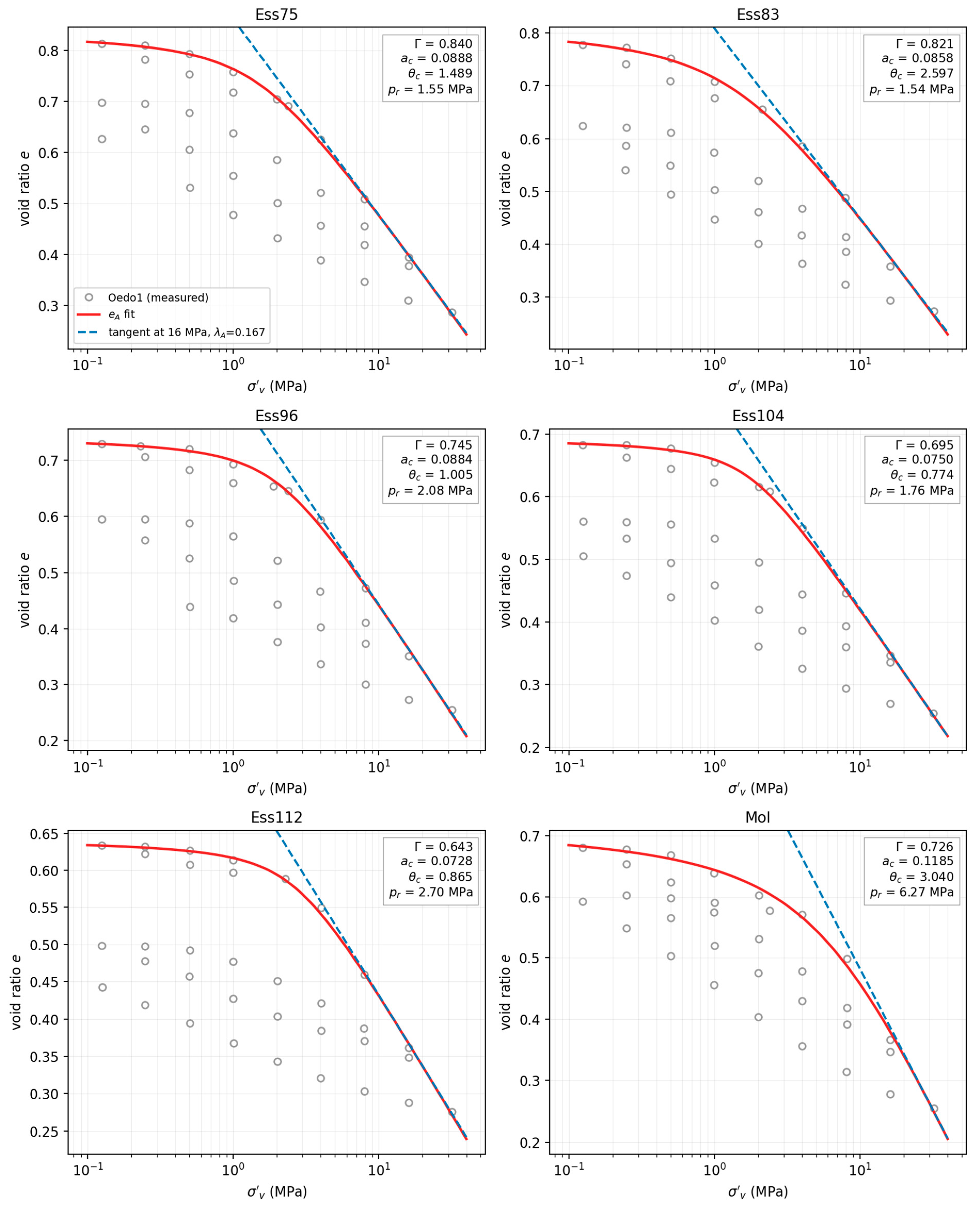
Before any paired-response simulation, the AJOP compression map itself is anchored to laboratory compression data. Six high-pressure Oedometer tests on Boom Clay reported by Deng et al. [39], five on cores from the Essen-1 borehole between approximately 219 m and 256 m depth and one on a core from the HADES underground laboratory at Mol, provide first-loading compression curves over the vertical effective stress range of 0.125–32 MPa. This window is wide enough to expose both regimes that $e_A$ is constructed to unify: the curved low-stress regime below and around the preconsolidation stress, and the log-linear regime at high stress. For each core, the nine-point first-loading envelope was extracted from the digitised test record and $e_A$ was fitted by unconstrained least squares over ($\Gamma$, $a_c$, ${\theta }_c$, $p_r$), with residuals measured in void ratio.

Figure 10 shows the six fits. The root-mean-square misfit lies between 3.7 × 10⁻³ and 7.7 × 10⁻³ in void ratio, with a single smooth curve per core tracking the data from the curved regime through the high-stress asymptote. The dashed lines show the tangent of $e_A$ at 16 MPa or 32 MPa; the corresponding tangent slopes ${\lambda }_A$ = 0.137–0.199 are consistent with the compression indices reported in [39] for the same tests ($C_c$ = 0.302–0.405, equivalent to slopes of 0.131–0.176 in natural logarithm). The tangent slopes slightly exceed the reported secant-type indices because ${\lambda }_A$ is still rising toward its asymptotic value $2a_c$ at the maximum applied stress, which is the limit behaviour stated in Theorem 1 made directly visible by the data. The fitted reference pressures $p_r$ = 1.5–6.3 MPa locate the curvature transition at a characteristic stress scale of the deposit; because the source warns that the Oedometer yield stress is stress-path dependent, this is not an independent preconsolidation-stress validation.

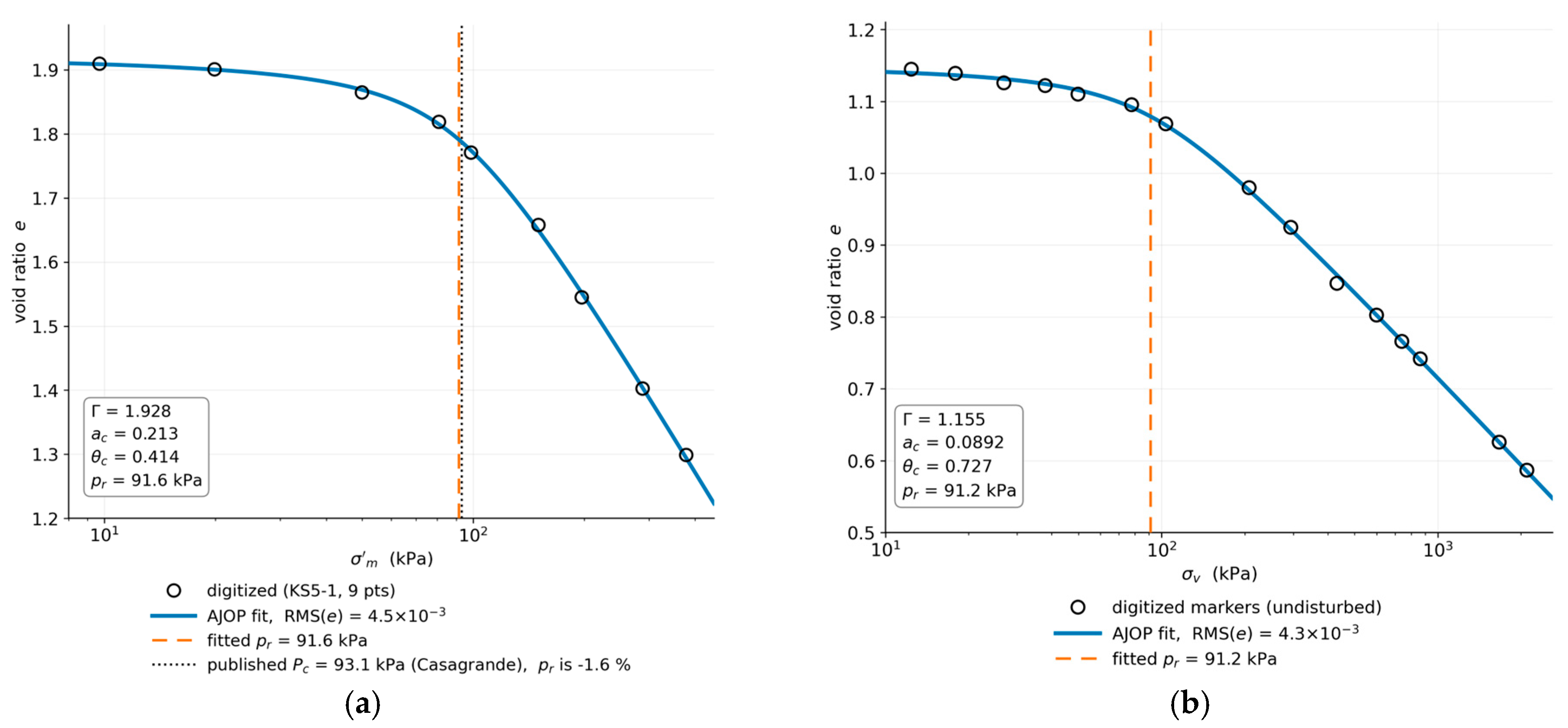
The same free four-parameter protocol was applied to two further natural clays digitised from the literature: the isotropic consolidation curve of sensitive Eastern Osaka clay (test KSS5-1 of [33]) and the Oedometer curve of undisturbed Shanghai clay, layer 4 [40] (Figure 11). In both cases, the fitted reference pressure lands on the independently reported yield stress without being told about it: $p_r$ = 91.6 kPa against the Casagrande value $P_c$ = 93.1 kPa reported in [33] (−1.6%), and $p_r$ = 91.2 kPa against the consolidation yield stress marked near 90–100 kPa in [40]. For the Osaka clay the measured high-stress slope of the digitised curve (0.374) reproduces the published $\lambda$ = 0.355 to 5%, fixing the natural-logarithm basis of that value; the fitted asymptote is $2a_c$ = 0.425, still above the data window—the test range ends inside the transition zone, so the curvature of the map is exercised, not merely its limit. The Shanghai fit gives $2a_c$ = 0.179 against the intrinsic compression index $\lambda$ = 0.140 carried by the structured-soil model of [40]; the difference is consistent with structured response over the tested range. Without an explicit structure variable, the single smooth map absorbs that discrepancy but does not identify its cause.

A note on identifiability closes the compression protocol. For the nine-point Osaka fit, the linearised one-sigma intervals are $\Gamma \pm 0.008$, $a_c\pm 0.008$, ${\theta }_c\times /÷1.23$ and $p_r\times /÷1.055$, with strong correlations ($a_c-p_r$ + 0.97, ${\theta }_c-\Gamma$ + 0.88): the four parameters are locally estimable within the linearised fit, but $a_c$ and $p_r$ trade against each other along the asymptote direction—which is exactly why the fitted $2a_c$ is declared to sit above the data window rather than claimed as measured. The most direct local anchor is $p_r$: estimated to ±5.5% at one sigma, it comfortably brackets the −1.6% gap to the published Casagrande value.

The Osaka program continues into undrained triaxial response: five compression paths (TSK series) and one extension path (TS6-2) digitised from [33] (Figure 12). Provenance follows the compression protocol: $M$ = 1.279 from the published $\phi \prime$ = 31.8°, $\kappa$ = 0.0477 published, $M_e$ = 0.897 implied by the SMP mapping and never fitted, and $\Psi$ = 1.4, $\Omega$ = 1.45 calibrated against the compression paths by a declared grid sweep. At this calibration, the two tests consolidated far beyond the yield stress are captured almost exactly (path-shape misfits 0.5–0.7% of ${p\prime }_0$, strengths −0.8% and −2.1%), while the tests at and near the yield stress are underpredicted by 15–31%: a single shared parameter pair cannot remove this trade-off. Recalibrating at ($\Psi$, $\Omega$) = (1.1, 2.2) reverses the pattern—the near-yield tests are then matched, and the extension strength is predicted to −4.0% with no extension-side information, while the far-from-yield strengths are overpredicted by about 20%. The displacement between these two calibrations, common in direction with the Bangkok clay below, is consistent with omitted destructuration or state-dependent fabric but does not identify a unique mechanism; the extension data of Figure 12b accordingly run left of the model endpoint.

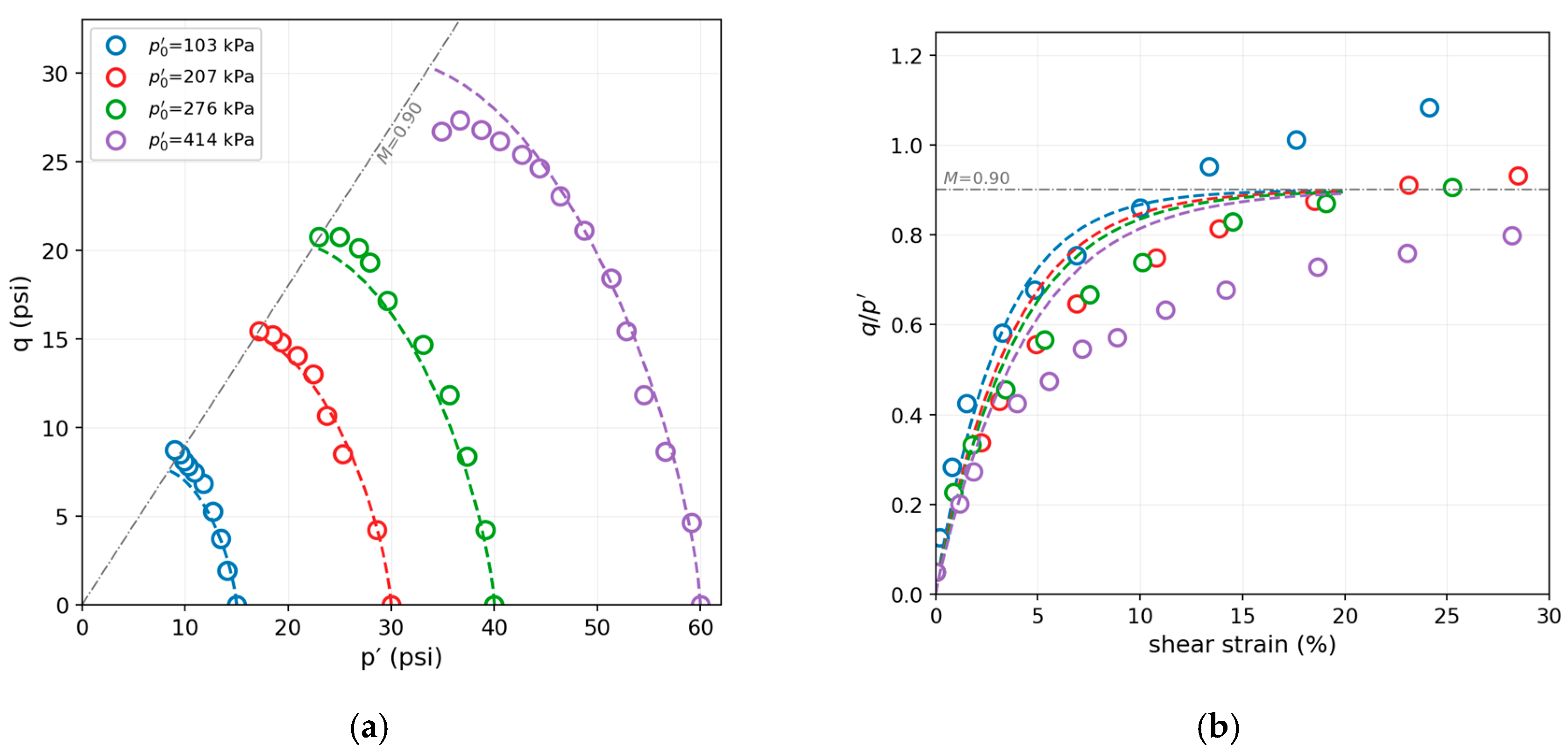
Weathered Bangkok clay [41] provides four nominally normally consolidated undrained triaxial tests at p′₀ = 103–414 kPa and a matching isotropic consolidation curve (Figure 13). The fitted map gives p_r = 29 kPa versus the reported yield knee near 40 kPa and places all tests on the high-stress asymptote. AJOP-T therefore coincides to three significant digits with its paired constant-slope form λ = 2a_c; only AJOP-T is drawn because the paired curves overlie it. The published λ = 0.51 is retained as an external scalar comparison, not plotted as another path. Compression RMS is 23.3 × 10⁻³ in void ratio, or 0.037 after normalisation by 2a_c, within the Boom Clay band 0.021–0.059. With M = 0.90 and κ = 0.12 from [41], and Ψ = 1.4 and Ω = 1.45 fitted by the declared grid sweep, path-shape RMS is 1.9% of p′₀ and strength endpoints lie within ±8%. Remaining discrepancies include a strain-scale mismatch of unresolved cause (possible time effects) and the decline in measured failure ratio from 1.01 to 0.76, which no single-M surface reproduces.

Table 2 collects the data-anchored calibrations for four natural clays, with the provenance of every number stated.

6.4. Overconsolidated Verification and Parameter Sensitivity

Twenty-four undrained paths were integrated at consolidation stresses of 100, 200 and 400 kPa, at OCR = 1, 2, 4, and 8, in compression and extension. With fixed void ratio, Equation (37) supplies the model-parameter-determined critical-state mean stress without path-specific fitting.

Table 3. Overconsolidated undrained paths at 400 kPa compared with Equation (37).

OCR	Mode	p′cs Computed (kPa)	Equation (37) (kPa)	Error (%)	Stationarity
1	TC/TE	217.5080	217.5080	0.0000	0
2	TC	401.1614	401.2390	−0.0193	2.5 × 10−8
2	TE	401.1750	401.2390	−0.0160	0
4	TC	740.4749	741.8229	−0.1817	2.2 × 10−7
4	TE	740.8153	741.8229	−0.1358	1.6 × 10−7
8	TC	1347.8388	1372.4078	−1.7902	2.0 × 10−6
8	TE	1355.2715	1372.4078	−1.2486	1.4 × 10−6

reports the most demanding set at 400 kPa; every path reached axial strain 0.240 with increments of 4 × 10⁻⁶, and terminal stationarity was at most 2 × 10⁻⁶.

The normally consolidated paths reproduce Equation (37) to every printed digit in both modes, with a terminal stress ratio equal to M, which is the numerical statement of Proposition 2. The overconsolidated paths approach the same locus from one side and depart from it by 0.019, 0.18 and 1.79 per cent at overconsolidation ratios of 2, 4, and 8, respectively. The departure is systematic rather than erratic, and its origin is the interpolation of the plastic modulus: an overconsolidated state approaches the critical state asymptotically through the mapping rule rather than reaching it, so a finite strain terminates the path slightly inside the locus. Equation (37) is therefore an attractor for overconsolidated states and an identity for normally consolidated ones, and the distinction is now quantified rather than asserted.

Across all twenty-four paths, the mean absolute departure from Equation (37) is 0.0000%, 0.0084%, 0.0746%, and 0.6825% at OCR = 1, 2, 4, and 8, with maxima of 0.0000%, 0.0193%, 0.1817%, and 1.7902%. Compression and extension behave alike: their twelve-path means are 0.2246% and 0.1581%, respectively.

Figure 3 and Figure 4 show parameter geometry; response sensitivities use central differences at ±10%, one factor at a time, while the admissibility boundary uses ±25%. Three results follow. The vertical intercept has a sensitivity of zero to three decimal places at every stress level for the undrained strength used here as the response metric. It positions the compression curve in the void-ratio direction and so does not enter that particular response, although it of course sets the ordinate of the compression and critical state lines themselves. This conditional OAT zero assumes fixed companions; it does not negate the joint intercept–roundness fit correlation in Section 6.3. The reference stress is the most influential parameter at low stress and the least at high stress, its sensitivity falling from 0.49 to 0.004 between 50 and 400 kPa, because it locates the transition and has little influence far from it. A quarter increase in it moves the admissibility boundary from 41.5 to 51.9 kPa and places a state at 50 kPa outside the admissible domain, which is the sharpest illustration in this paper that the boundary of Proposition 1 is a calibration statement and not a formality. At 400 kPa, no sensitivity exceeds 0.081. Above the transition, reference-stress and roundness sensitivities collapse while classical slope and swelling dependence remains, consistent with Theorem 1.

Table 4. Logarithmic sensitivity of the undrained strength to each calibrated parameter, and the effect of each on the admissibility boundary.

Parameter	S at 50 kPa	S at 100 kPa	S at 200 kPa	S at 400 kPa	p′* at −25%/Base/+25% (kPa)
Γ	0.000	0.000	0.000	0.000	41.50/41.50/41.50
ac	−0.249	−0.118	−0.086	−0.081	48.63/41.50/36.33
θc	−0.102	0.010	0.007	0.003	46.14/41.50/37.80
p′r	0.491	0.136	0.017	0.004	31.12/41.50/51.87
κ	0.247	0.117	0.085	0.080	34.89/41.50/46.98

Note: * denotes the mean effective stress corresponding to the admissibility boundary u* in Proposition 1; p′* = p_r exp(u*).

gives the logarithmic sensitivity S = dln(s_u)/dln(parameter), estimated by central difference at plus and minus ten per cent with the remaining four parameters held at the Eastern Osaka calibration, together with the effect of a quarter change in each parameter on the admissibility boundary of Proposition 1. The response metric is the undrained strength in compression; sensitivities to other response measures are not implied by these numbers.

7. Discussion

7.1. Why the Formulation Is Mathematical Rather than Descriptive

AJOP-T is defined by the inherited bounding-surface machinery (Section 2), the AJOP derivative hierarchy (Section 3), a closed-form admissible hardening domain, the consistency condition and elasto-plastic tangent (Section 4), and the structural results of Section 5. It is therefore a high-order mathematical constitutive formulation in the sense of the Mathematics precedent [8], not a descriptive model comparison.

AJOP is used here as a differentiable hardening map rather than a settlement equation: its first derivative replaces the constant compression index, and its second controls the stress sensitivity of the hardening modulus. Theorem 2 recovers the settlement equation of [24] as the isotropic NC restriction, linking the constitutive and settlement formulations.

7.2. Difference from Fractional, Gradient, and EVP Formulations

Here, high-order does not denote strain-gradient plasticity [42], fractional plasticity [43], or an EVP/creep model [44]; AJOP-T adds no extra boundary conditions, nonlocal length scale, fractional derivative or rate dependence. It refers only to successive derivatives of the smooth compression map: $e_A$, ${\lambda }_A$ and ${\chi }_A$.

Relative to Modified Cam Clay {$\lambda$, $\kappa$, $M$, $N$}, the teardrop base model adds $\Psi$ and $\Omega$ [10], while AJOP-T replaces {$\lambda$, $N$} with {$\Gamma$, $a_c$, ${\theta }_c$, $p_r$}. This net increase of two degrees of freedom is identified from the same compression curve that calibrates $\lambda$ and $N$, without an additional test; Section 6.3 addresses identifiability. Theorem 1 nests the constant-slope model: at high stress the map collapses to $\lambda =2a_c$ and the intercept, confining the added freedom to low-stress curvature.

7.3. Relation to Recent Clay Constitutive Models

Recent clay models modify different parts of the constitutive architecture. Tong et al. [8] changed stress-dilatancy and yield geometry through a high-order yield function, whereas Xu et al. [9] developed a unified plastic potential for overconsolidated clays. Yao, Hou and Zhou [45] and Jocković and Vukićević [46] evolved hardening to reach overconsolidated states at Modified Cam Clay parameter cost; SANICLAY [47] instead evolves surface orientation. Chatwong et al. [10] introduced the continuous teardrop bounding surface with symmetric curvature control. AJOP-T changes only the compression-derived hardening law while preserving that surface structure; Remark 3 shows that the two modifications act on orthogonal parts of the formulation.

In boundary-value problems, the difference between curved and constant-slope compression is spatially localised: shallow elements can remain on the curved branch, whereas deep elements approach the constant-slope regime (Figure 9a; Section 6.2). Because surface loading also concentrates its settlement influence near the surface, AJOP-T should differ most there and converge with the constant-slope prediction at depth. The compression fit therefore estimates the transition depth before the finite element analysis.

7.4. Scope Assumptions and Phased Extensions

Two control assumptions bound this phase: rate-independent skeleton and constant κ; neither is universal. Proposition 2 is exact only for normally consolidated bounding-surface paths (overconsolidated paths approach it asymptotically; Section 6.4), destructuration is absent, four compression maps and the reported triaxial paths are fitted, only one Eastern Osaka extension is held out, and no field data are used. Claims concern the stated monotonic and single unload–reload paths and comparative boundary-value tests; reference-clay extension [10] is deferred.

Constant κ is inherited, not a universal unload–reload law. With no stress-dependent data, 0.5–2.0 times calibration is sensitivity, not bias. From Δe^e = −κ ln(p′₂/p′₁), elastic increment scales by −50% to +100%; P₀ is unchanged until plasticity. Plastic-reloading sensitivity κ/(λ_A−κ) is 2.47, 0.246, 0.145, and 0.132 at 50, 100, 200, and 400 kPa. Applicability is calibration-specific: p′ > p′* and a sensitivity buffer are mandatory. For Eastern Osaka, 100–400 kPa is lower-sensitivity and 50 kPa near-boundary; the envelope moves the boundary to 26–60 kPa and the 50 kPa paired strength difference to 17.6–30.5%. These are bounds, not validated bias. A separate phase in development targets stress-/history-dependent swelling, accumulated volumetric strain and cyclic re-yield.

Triaxial results expose a limitation consistent with omitted destructuration or state-dependent fabric: Osaka predicts a +1.6 per cent strength-ratio change against roughly ±20 per cent scatter, while Bangkok measurements decline although a single-M surface is constant, limiting endpoint agreement to ±8 per cent. Calibrations cluster near (Ψ, Ω) ≈ (1.4, 1.4–1.5) but require larger Ω near yield, a discrepancy that such mechanisms could absorb.

Rate independence isolates hardening and keeps Theorem 2 comparable to [24]. The Bangkok mismatch may include time effects; rate is unreported, so creep is unidentified. A separate EVP/overstress or equivalent-time phase [44] in development requires new equations and verification; no time-dependent prediction follows.

7.5. Implementation in a Finite Element Framework

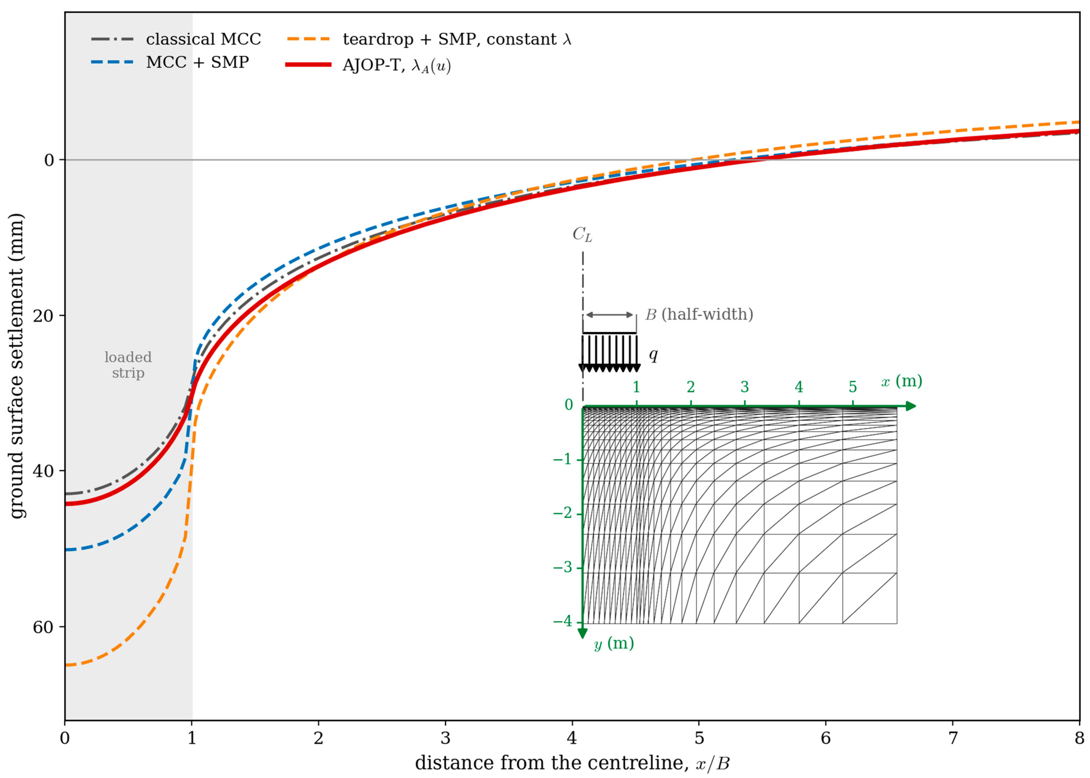
An independent script, a source-tree stress-point driver and a single-element finite-element analysis agree to at least five significant figures for Eastern Osaka paths from 50 to 800 kPa. Proposition 1 is enforced: 50 kPa integrates, whereas 25 kPa, below the 41.5 kPa boundary, is rejected. Figure 14 gives the footing comparison.

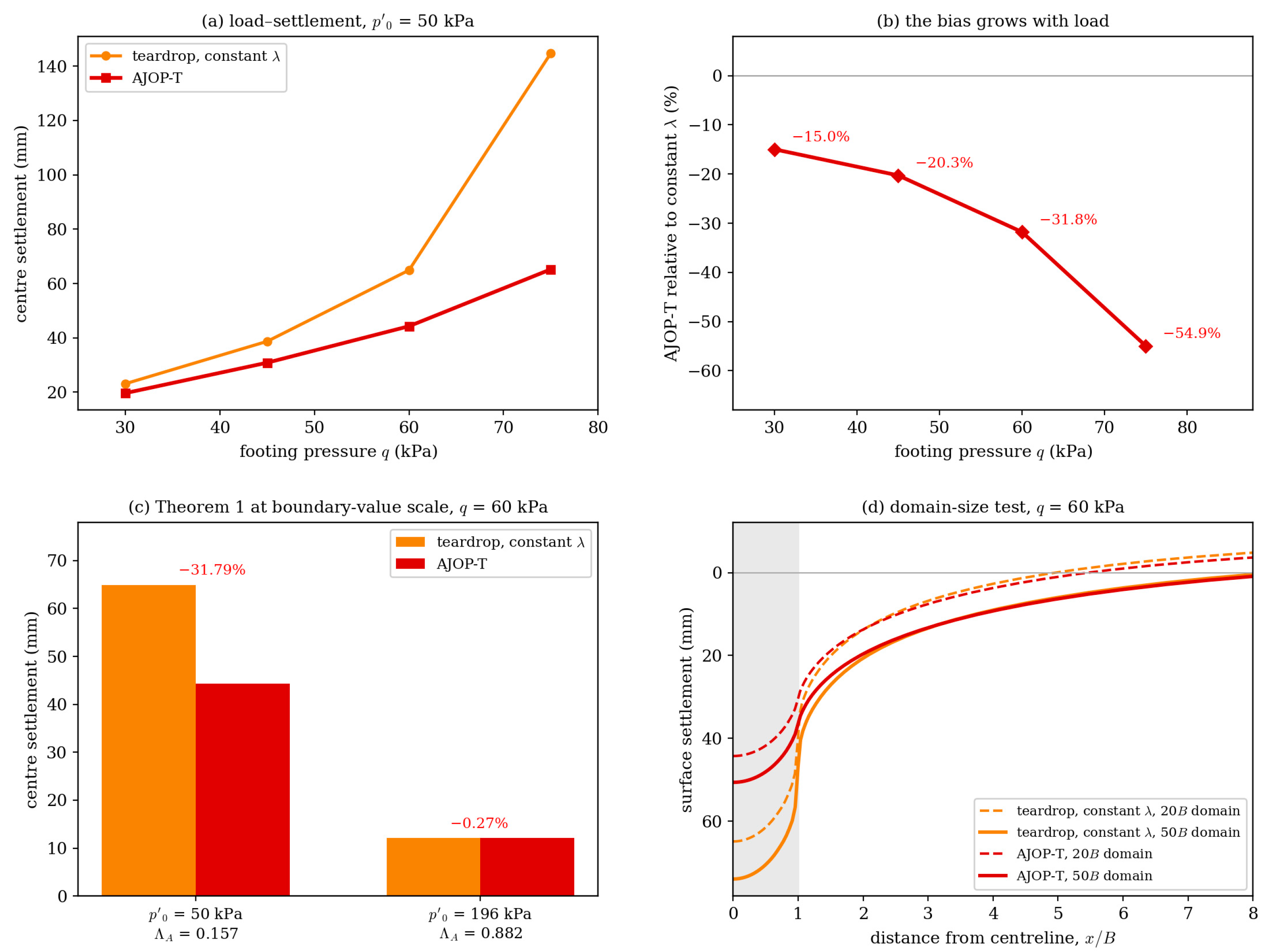
Uniform traction q = 60 kPa acts over the footing half-width in the paired stress-level comparison. Four configurations share mesh, elasticity, strength, swelling index, and initial state, differing only in yield/flow geometry, the deviatoric criterion or hardening law. For the initial NC mean effective stress p′₀ = 50 kPa, equal to the initial preconsolidation size (normalised tangent modulus 0.157), AJOP hardening reduces centre settlement by 31.8 per cent relative to its constant-slope twin; for the paired near-asymptotic initial state p′₀ = 196 kPa (0.882), settlement and trough-shape differences fall to 0.27 and 0.2 per cent. This recovers Theorem 1 at boundary-value scale.

The hardening-law difference is load dependent rather than a fixed bias (Figure 15a,b): across footing pressures of 30, 45, 60, and 75 kPa it grows from 15 to 55 per cent. Over the same range, normalised settlement increases by factors of 2.5 for the constant-slope model and 1.3 for AJOP-T; the former concentrates deformation beneath the strip, whereas the latter continues to recruit the surrounding deposit. The tested domain enlargement does not explain the paired difference (Figure 15d): enlarging both mesh dimensions by a factor of 2.5 changes each settlement by 14 per cent but their relative difference by only 0.2 percentage points. Because the absolute trough extent is not converged at either size, it is not reported.

The closed-form second derivative supplies the constitutive derivative for the local Jacobian, while admissibility is checked before integration. Because geometry, mapping and transformed stress are unchanged, so are element assembly, the global solve and the stress-point iteration structure; each evaluation adds one square root and its derivatives. On one core, with 1440 six-noded triangles and 8967 degrees of freedom, runtime is 1.11 times that of Modified Cam Clay. The local root-finder is called 10,830 times versus 97,618 for the constant-slope member, with worst-case counts of five and seven iterations, reducing root-finder workload in this run. Settlements are unchanged to printed digits from 40 to 160 substeps. A discretisation-consistent algorithmic tangent has not been derived, so asymptotically quadratic global Newton convergence is not claimed. Raising the local iteration limit until every substep converges changes the constant-slope and MCC-with-SMP settlements by 0.059 and 0.055 per cent, and the hardening-law difference from 31.80 to 31.83 per cent. AJOP-T required no forced substep acceptance; its algorithmic tangent is the next implementation step.

Near-boundary conditioning was tested from states 0.1, 1, 5, 15 and 40 per cent above the boundary, and at higher stress multiples, for three numerical parameter sets with boundaries of 41.5, 26.2 and 35.3 kPa and swelling ratios differing threefold. At the closest state, the hardening denominator falls to 8.3 × 10⁻⁵ and 1.5 × 10⁻⁵ in two of the parameter sets. Error against eightfold-refined integration is 7.2 × 10⁻⁵ there and 5.6 × 10⁻⁵ at a state 2000 times farther from the boundary, with no measurable timing change. No degradation was observed for these three parameter sets, paths and increment controls; this is not a general proof of conditioning. States below the boundary are rejected before integration.

The formulation uses effective stress and assumes full saturation; with w = e/G_s, water content follows from void ratio and specific gravity rather than acting as an independent constitutive variable. Rate independence concerns the soil skeleton. Although the footing analyses use a coupled displacement-pore-pressure formulation, they are evaluated undrained: drainage is suppressed, and pore pressure enforces constant volume. The examples therefore test constitutive integration and the paired hardening laws, not permeability or consolidation time.

7.6. Experimental Detectability of the Predicted Low-Stress Strength Drift

The curved critical-state line of Proposition 2 and the stress dependence of the undrained strength ratio in Section 5.4 arise from the hardening law; no undrained strength enters the compression calibration. They are therefore falsifiable predictions. A discriminating test would use reconstituted clay at low consolidation stress while controlling preparation-induced fabric. Existing low-stress triaxial evidence includes both confounded and non-supporting results.

Hong et al. [48] tested three reconstituted clays, isotropically consolidated from initial water contents of one to two liquid limits; their undrained strength ratios span 0.28–0.60. This preparation effect exceeds the predicted drift by more than an order of magnitude. Shi et al. [49] showed that consolidation path changes the response and normalised strength ratio at the same mean effective stress, while Bian et al. [50] found that initial water content changes the critical-state line. Stress path and preparation must therefore be controlled together; these datasets do not isolate stress-level curvature at fixed preparation.

Yin et al. [51] reported straight strength envelopes through the origin within each preparation series of K₀-consolidated reconstituted Lianyungang clay, while the normalised strength decreased with initial water content. This supports stress-level independence within a series and confirms preparation as a strong confounder. However, the K0 path differs from the isotropic path of Proposition 2, the tested range is not located relative to the compression reference stress, and no uncertainty is reported at the required approximately 1 per cent resolution. The data show no drift of the predicted size but cannot establish that it is zero.

For Eastern Osaka clay, the predicted drift is about 1.6 per cent, whereas the same strength data vary by roughly 20 per cent and the Bangkok endpoints are constrained only to about 8 per cent. The signal is therefore about an order of magnitude below the inter-test spread and is retained as a falsifiable theoretical prediction, not an experimentally demonstrated improvement. The principal hardening result does not depend on this drift; it follows from the compression map, Theorems 1 and 2, and the boundary-value results of Section 7.5.

The relevant test range is material-specific: consolidation stress must span the transition regime around the material’s compression reference stress, not a fixed absolute interval. Far above it, Theorem 1 recovers constant-slope response, and no improvement is expected. A decisive test would require reconstituted material at one preparation water content, isotropic consolidation from below to well above the reference stress, constant strain rate, and enough replication to resolve about a 1 per cent change in strength ratio. None of the reviewed datasets meets all these conditions.

8. Conclusions

AJOP-T replaces the constant critical-state hardening slope with the AJOP tangent modulus while retaining the teardrop bounding surface, non-associated flow, radial mapping and SMP transformed stress. It is therefore a stress-dependent hardening law, not a new yield geometry or flow rule.

The derivative hierarchy yields the void-ratio law, tangent modulus and stress sensitivity; it recovers constant-slope hardening (Theorem 1), the parent isotropic NC settlement equation (Theorem 2) and the explicit admissibility boundary (Proposition 1), while leaving the hardening hierarchy invariant under SMP (Remark 3). Proposition 2 and the stress-dependent strength ratio remain predictions, not calibration targets.

Evidence comprises four-clay compression fits, fitted Osaka compression and Bangkok paths, and one held-out Osaka extension. Three computational paths—one independently implemented—agree to five significant figures; 24 overconsolidated paths depart from the derived critical-state line by at most 1.79 per cent, and no degradation was observed in the reported near-boundary tests. Footing runtime is 1.11 times that of Modified Cam Clay, with no forced substep acceptance. The settlement reduction shifts from 31.8 per cent in the curved regime to 0.27 per cent near the asymptote, confining the effect to the transition range.

Field superiority is not established: only one path is held out and no field data are used. This first phase assumes rate independence and constant κ, omits destructuration, and lacks a discretisation-consistent algorithmic tangent. The predicted 1.6 per cent strength drift remains unvalidated. Follow-on phases address time dependence, cyclic swelling and field validation.

References

1. Roscoe, K.H.; Schofield, A.N.; Thurairajah, A. Yielding of clays in states wetter than critical. Géotechnique 1963, 13, 211–240. [Google Scholar] [CrossRef] [Scilit]
2. Roscoe, K.H.; Burland, J.B. On the generalized stress–strain behaviour of wet clay. In Engineering Plasticity; Heyman, J., Leckie, F.A., Eds.; Cambridge University Press: Cambridge, UK, 1968; pp. 535–609. [Google Scholar]
3. Schofield, A.N.; Wroth, C.P. Critical State Soil Mechanics; McGraw-Hill: London, UK, 1968. [Google Scholar]
4. Wood, D.M. Soil Behaviour and Critical State Soil Mechanics; Cambridge University Press: Cambridge, UK, 1990. [Google Scholar]
5. Vermeer, P.A.; de Borst, R. Non-associated plasticity for soils, concrete and rock. Heron 1984, 29, 1–64. [Google Scholar]
6. Rowe, P.W. The stress-dilatancy relation for static equilibrium of an assembly of particles in contact. Proc. R. Soc. Lond. A 1962, 269, 500–527. [Google Scholar] [CrossRef] [Scilit]
7. Li, X.S.; Dafalias, Y.F. Dilatancy for cohesionless soils. Géotechnique 2000, 50, 449–460. [Google Scholar] [CrossRef] [Scilit]
8. Tong, C.-X.; Liu, H.-W.; Li, H.-C. Constitutive modeling of normally and over-consolidated clay with a high-order yield function. Mathematics 2022, 10, 1376. [Google Scholar] [CrossRef] [Scilit]
9. Xu, B.; Chen, K.; Pang, R. A bounding surface model for overconsolidated clays with unified plastic potential function in triaxial and general stress state. Comput. Geotech. 2024, 172, 106429. [Google Scholar] [CrossRef] [Scilit]
10. Chatwong, T.; Kaewhanam, N.; Kaewplang, S.; Phonchamni, N.; Inthidech, S.; Kampala, A.; Sultornsanee, S. A robust constitutive model for clays over a wide range of plasticity and overconsolidation ratio (OCR) with symmetric, continuous curvature control of a teardrop yield surface. Symmetry 2026, 18, 215. [Google Scholar] [CrossRef] [Scilit]
11. Dafalias, Y.F.; Herrmann, L.R. Bounding surface formulation of soil plasticity. In Soil Mechanics—Transient and Cyclic Loads; Pande, G.N., Zienkiewicz, O.C., Eds.; John Wiley and Sons: Chichester, UK, 1982; pp. 253–282. [Google Scholar]
12. Dafalias, Y.F.; Herrmann, L.R. Bounding surface plasticity. II: Application to isotropic cohesive soils. J. Eng. Mech. 1986, 112, 1263–1291. [Google Scholar] [CrossRef] [Scilit]
13. Dafalias, Y.F. Bounding surface plasticity. I: Mathematical foundation and hypoplasticity. J. Eng. Mech. 1986, 112, 966–987. [Google Scholar] [CrossRef] [Scilit]
14. Hashiguchi, K. Subloading surface model in unconventional plasticity. Int. J. Solids Struct. 1989, 25, 917–945. [Google Scholar] [CrossRef] [Scilit]
15. Nagaraj, T.S.; Srinivasa Murthy, B.R. Rationalization of Skempton’s compressibility equation. Géotechnique 1983, 33, 433–443. [Google Scholar] [CrossRef] [Scilit]
16. Skempton, A.W.; Jones, O.T. Notes on the compressibility of clays. Q. J. Geol. Soc. Lond. 1944, 100, 119–135. [Google Scholar] [CrossRef] [Scilit]
17. Butterfield, R. A natural compression law for soils. Géotechnique 1979, 29, 469–480. [Google Scholar] [CrossRef] [Scilit]
18. Burland, J.B. On the compressibility and shear strength of natural clays. Géotechnique 1990, 40, 329–378. [Google Scholar] [CrossRef] [Scilit]
19. Hong, Z.S.; Zeng, L.L.; Cui, Y.J.; Cai, Y.Q.; Lin, C. Compression behaviour of natural and reconstituted clays. Géotechnique 2012, 62, 291–301. [Google Scholar] [CrossRef] [Scilit]
20. Horpibulsuk, S.; Liu, M.D.; Zhuang, Z.; Hong, Z.S. Complete compression curves of reconstituted clays. Int. J. Geomech. 2016, 16, 06016005. [Google Scholar] [CrossRef] [Scilit]
21. Pestana, J.M.; Whittle, A.J. Compression model for cohesionless soils. Géotechnique 1995, 45, 611–631. [Google Scholar] [CrossRef] [Scilit]
22. Liu, M.D.; Carter, J.P. A structured Cam Clay model. Can. Geotech. J. 2002, 39, 1313–1332. [Google Scholar] [CrossRef] [Scilit]
23. Kaewhanam, N.; Chaimoon, K. A simplified silty sand model. Appl. Sci. 2023, 13, 8241. [Google Scholar] [CrossRef] [Scilit]
24. Phonchamni, N.; Chatwong, T.; Udomchai, A.; Sultornsanee, S.; Angkawisittpan, N.; Sangiamsak, N.; Kaewhanam, N. Refined consolidation settlement calculation based on the oedometer tests for normally and overconsolidated clays. Appl. Sci. 2025, 15, 5777. [Google Scholar] [CrossRef] [Scilit]
25. Leroueil, S.; Kabbaj, M.; Tavenas, F.; Bouchard, R. Stress–strain–strain rate relation for the compressibility of sensitive natural clays. Géotechnique 1985, 35, 159–180. [Google Scholar] [CrossRef] [Scilit]
26. Grimstad, G.; Degago, S.A.; Nordal, S.; Karstunen, M. Modeling creep and rate effects in structured anisotropic soft clays. Acta Geotech. 2010, 5, 69–81. [Google Scholar] [CrossRef] [Scilit]
27. Ding, P.; Ju, L.; Xu, R.; Yan, Z.; Wu, M.; Zhang, G. An egg-shaped elastic viscoplastic model for clay: Experimental investigation and constitutive modelling. KSCE J. Civ. Eng. 2023, 27, 1993–2003. [Google Scholar] [CrossRef] [Scilit]
28. Oathes, T.J.; Boulanger, R.W.; Ziotopoulou, K. A viscoplastic constitutive model for plastic silts and clays for static slope stability applications. Can. Geotech. J. 2024, 61, 2553–2570. [Google Scholar] [CrossRef] [Scilit]
29. Song, P.; Buscarnera, G. SANICLAY-RD: A model for rate-dependent effects under complex loading paths. Comput. Geotech. 2025, 187, 107457. [Google Scholar] [CrossRef] [Scilit]
30. Matsuoka, H.; Nakai, T. Stress-deformation and strength characteristics of soil under three different principal stresses. Proc. Jpn. Soc. Civ. Eng. 1974, 232, 59–70. [Google Scholar] [CrossRef] [Scilit] [PubMed]
31. Nakai, T.; Matsuoka, H. A generalized elastoplastic constitutive model for clay in three-dimensional stresses. Soils Found. 1986, 26, 81–98. [Google Scholar] [CrossRef] [Scilit] [PubMed]
32. Matsuoka, H.; Yao, Y.-P.; Sun, D.A. The Cam-clay models revised by the SMP criterion. Soils Found. 1999, 39, 81–95. [Google Scholar] [CrossRef] [Scilit]
33. Adachi, T.; Oka, F.; Hirata, T.; Hashimoto, T.; Nagaya, J.; Mimura, M.; Pradhan, T.B.S. Stress-strain behavior and yielding characteristics of Eastern Osaka clay. Soils Found. 1995, 35, 1–13. [Google Scholar] [CrossRef] [Scilit]
34. Borja, R.I.; Lee, S.R. Cam-Clay plasticity, Part 1: Implicit integration of elasto-plastic constitutive relations. Comput. Methods Appl. Mech. Eng. 1990, 78, 49–72. [Google Scholar] [CrossRef] [Scilit]
35. Sloan, S.W.; Abbo, A.J.; Sheng, D. Refined explicit integration of elastoplastic models with automatic error control. Eng. Comput. 2001, 18, 121–194. [Google Scholar] [CrossRef] [Scilit]
36. Mayne, P.W. Cam-clay predictions of undrained strength. J. Geotech. Eng. Div. ASCE 1980, 106, 1219–1242. [Google Scholar] [CrossRef] [Scilit]
37. Ladd, C.C.; Foott, R. New design procedure for stability of soft clays. J. Geotech. Eng. Div. ASCE 1974, 100, 763–786. [Google Scholar] [CrossRef] [Scilit]
38. Wroth, C.P. The interpretation of in situ soil tests. Géotechnique 1984, 34, 449–489. [Google Scholar] [CrossRef] [Scilit]
39. Deng, Y.F.; Tang, A.M.; Cui, Y.J.; Nguyen, X.P.; Li, X.L.; Wouters, L. Laboratory hydro-mechanical characterisation of Boom Clay at Essen and Mol. Phys. Chem. Earth 2011, 36, 1878–1890. [Google Scholar] [CrossRef] [Scilit]
40. Ye, G.-L.; Ye, B. Investigation of the overconsolidation and structural behavior of Shanghai clays by element testing and constitutive modeling. Undergr. Space 2016, 1, 62–77. [Google Scholar] [CrossRef] [Scilit]
41. Balasubramaniam, A.S.; Hwang, Z.-M. Yielding of weathered Bangkok clay. Soils Found. 1980, 20, 1–15. [Google Scholar] [CrossRef] [Scilit] [PubMed]
42. Aifantis, E.C. On the microstructural origin of certain inelastic models. J. Eng. Mater. Technol. 1984, 106, 326–330. [Google Scholar] [CrossRef] [Scilit]
43. Sun, Y.; Xiao, Y. Fractional order plasticity model for granular soils subjected to monotonic triaxial compression. Int. J. Solids Struct. 2017, 118–119, 224–234. [Google Scholar] [CrossRef] [Scilit]
44. Yin, J.-H.; Graham, J. Equivalent times and one-dimensional elastic viscoplastic modelling of time-dependent stress–strain behaviour of clays. Can. Geotech. J. 1994, 31, 42–52. [Google Scholar] [CrossRef] [Scilit]
45. Yao, Y.-P.; Hou, W.; Zhou, A.-N. UH model: Three-dimensional unified hardening model for overconsolidated clays. Géotechnique 2009, 59, 451–469. [Google Scholar] [CrossRef] [Scilit]
46. Jocković, S.; Vukićević, M. Bounding surface model for overconsolidated clays with new state parameter formulation of hardening rule. Comput. Geotech. 2017, 83, 16–29. [Google Scholar] [CrossRef] [Scilit]
47. Dafalias, Y.F.; Manzari, M.T.; Papadimitriou, A.G. SANICLAY: Simple anisotropic clay plasticity model. Int. J. Numer. Anal. Methods Geomech. 2006, 30, 1231–1257. [Google Scholar] [CrossRef] [Scilit]
48. Hong, Z.S.; Bian, X.; Cui, Y.J.; Gao, Y.F.; Zeng, L.L. Effect of initial water content on undrained shear behaviour of reconstituted clays. Géotechnique 2013, 63, 441–450. [Google Scholar] [CrossRef] [Scilit]
49. Shi, J.; Qian, S.; Zeng, L.L.; Hong, Z.S. Undrained shear behaviors of reconstituted Wenzhou clay under different consolidation stress paths. Chin. J. Geotech. Eng. 2014, 36, 1674–1679. [Google Scholar] [CrossRef]
50. Bian, X.; Hong, Z.S.; Cai, Z.Y.; Zeng, L.L. Change of critical state lines of reconstituted clays with initial water contents. Chin. J. Geotech. Eng. 2013, 35, 164–169. [Google Scholar]
51. Yin, J.; Zhang, K.; Geng, W.; Gaamom, A.; Xiao, J. Effect of initial water content on undrained shear strength of K0 consolidated clay. Soils Found. 2021, 61, 1453–1463. [Google Scholar] [CrossRef] [Scilit]
Figure 1. Effect of the SMP transformed stress. (a) SMP locus versus the symmetric constant- M circle: coincidence in triaxial compression, separation in extension. (b) Single-variable ablation at the Eastern Osaka calibration [33]: compression paths coincide; the extension endpoint shifts from M to M e , where the latter denotes the positive magnitude of the SMP-implied extension ratio, a 43% strength difference. The blue circle and orange triangle indicate the TC and TE directions, respectively; the plus sign marks the origin.
Mathematics 14 02975 g001
Figure 2. Continuous teardrop surface: (a) isolated effect of Ψ at Ω = 1; (b) radial mapping. In (a), the grey dotted line is the CSL, the black dashed line joins the surface apices, and the arrows identify the apex locus and the Ψ = Ω = 1 coincidence. In (b), the black arrowed segments denote ℓ and L, the black dashed line is the radial mapping ray, and the coloured dotted guides project the coordinates of (p, q) and (P, Q).
Mathematics 14 02975 g002
Figure 3. AJOP compression map. (a) Roles of Γ , a c , θ c , and p r for Eastern Osaka. (b) Factored family: θ c controls shape; θ c 0 gives the bilinear limit.
Mathematics 14 02975 g003
Figure 4. Dimensionless AJOP hardening surface: (a) Λ A over u and θ c ; (b) χ A / χ A 0 on Λ A contours.
Mathematics 14 02975 g004
Figure 5. Admissible hardening domain of AJOP-T in the ρ κ , u plane for several roundness values θ c . The curve u ρ κ of Equation (26) separates the admissible domain Λ A > ρ κ (above) from the inadmissible domain (below).
Mathematics 14 02975 g005
Figure 6. Normalised undrained strength ratio of normally consolidated states, s u / p ~ 0 divided by its high-stress limit of Equation (41), as a function of the initial hardening coordinate u 0 for several roundness values θ c ( ρ κ = 0.2 , Ω = 1 ). The ratio is stress-level-independent only in the log-linear regime and rises in the curved regime toward a finite limit at the admissibility boundary (Corollary 2).
Mathematics 14 02975 g006
Figure 7. Nested family of teardrop bounding surfaces at increasing preconsolidation size P ~ 0 , each surface coloured by its own normalised tangent hardening modulus Λ A . Members are geometrically similar; colour shows the hardening transition of Equation (21), and the grey dashed line is the CSL q ~ = M p ~ .
Mathematics 14 02975 g007
Figure 8. Curvature-induced hardening trajectories h ^ s for a family of roundness values θ c on a common loading path.
Mathematics 14 02975 g008
Figure 9. Paired AJOP-T and constant- λ undrained response at the Eastern Osaka calibration. (a) Initial states and the admissibility boundary. (b) Effective stress paths. (c) Strength and path separation versus u 0 ; both vanish on the asymptote and grow toward the boundary. Shaded bands locate the Osaka and Bangkok tests. In (a), coloured circles mark the selected initial states along the AJOP map, and u* denotes the admissibility boundary of Proposition 1. In (b), colour identifies the initial state; solid and dashed curves denote AJOP-T and paired constant-λ paths, respectively. The black legend samples are line-style keys rather than additional data curves; the grey dotted line denotes η = M.
Mathematics 14 02975 g009
Figure 10. Boom Clay high-pressure Oedometer compression curves at Essen and Mol, digitised from Deng et al. [39]. Circles are data, solid curves are AJOP fits and dashed lines are high-stress tangents. Each panel reports Γ , a c , θ c , p r and the corresponding tangent slope.
Mathematics 14 02975 g010
Figure 11. Compression-map calibrations: (a) Eastern Osaka isotropic consolidation [33]; (b) Shanghai layer 4 Oedometer test [40]. Markers are digitised data, solid curves are AJOP fits and fitted p r values are compared with independently reported yield stresses.
Mathematics 14 02975 g011
Figure 12. Compression-anchored Eastern Osaka comparison, digitised from [33] and normalised by σ m 0 = 98 kPa. (a) Five compression paths; (b) held-out TS6-2 extension against the SMP-implied M e . Post-peak data are shown in grey; the mismatch does not identify a unique structural mechanism. Grey dotted lines denote the TC and SMP-implied TE critical-state ratios, M = 1.279 and −Me = −0.897.
Mathematics 14 02975 g012
Figure 13. Fitted comparison for nominally normally consolidated weathered Bangkok clay [41]. (a) Effective stress paths at four consolidation pressures: circles are digitised data and dashed curves are AJOP-T; the paired constant-slope response λ = 2ac is indistinguishable at the plotted scale. (b) Stress ratio versus shear strain. The four paths calibrated Ψ and Ω; details are given in Table 2. Grey dash-dotted lines denote the critical-state ratio M = 0.90.
Mathematics 14 02975 g013
Figure 14. Same-mesh strip-footing settlement at q = 60 kPa for initial NC p′0 = 50 kPa: classical MCC, MCC with SMP, teardrop plus SMP with constant λ, and AJOP-T with λA(u); inset: half-domain, load and mesh.
Mathematics 14 02975 g014
Figure 15. Boundary-value effect of hardening: (a) load-settlement curves; (b) signed paired-model relative difference (not error against observations); (c) curved and near-asymptotic regimes; (d) domain-size check at 60 kPa. Grey horizontal lines mark zero response or difference, and the grey shaded band in (d) marks the loaded footing half-width (0 ≤ x/B ≤ 1).
Mathematics 14 02975 g015