Hierarchical Bayesian Multi-Dimensional IRT Applied to 200k Concept Tests

Abstract

We report the use of our group’s hierarchical Bayesian implementation of the multi-dimensional nominal categories model followed by standard factor rotations of the principal dimensions to obtain 28 curated sparse dimensions from a set of 203,564 (104,998 pre- and 98,566 post-) administrations of a multiple-choice concept test in mechanics. We emphasize our careful attention to issues common to fitting such multi-parameter models to large datasets: a novel set of filters to remove administrations of questionable validity, the use of Bayesian methods to avoid overfitting, selecting the best transformations to find easily identifiable sparse dimensions, and verification and pruning of these using bootstrap samples. We demonstrate that these dimensions are invariant across demographically different samples of students as well as between pre-instruction and post-instruction samples. Most sparse dimensions correspond to well-known misconceptions in mechanics.

1. Introduction

Large-scale assessments in educational measurements and psychometrics routinely collect responses from thousands of testees on dozens of multiple-choice items, yielding high-dimensional categorical data. Here, we analyze a dataset of 203,564 administrations of the Force Concept Inventory (FCI), a pioneering research-designed multiple-choice instrument called a concept test [1]. In such instruments, distractors are designed from prior research on common student responses to be systematically attractive to students with corresponding patterns of reasoning. Presumably, students select particular choices logically, based on their belief in particular misconceptions that are incompatible with current scientific knowledge, and not because they are randomly guessing. If so, a misconception should manifest as a particular pattern of distractors (incorrect choices) selected by those students holding that specific misconception.

Thus, our working hypothesis was that the dimensional structure of the FCI consists of a primary Newtonian-correct dimension together with multiple additional dimensions, each corresponding to a particular misconception or misconception-like response pattern. Our objective in this paper was to develop methods for identifying as many misconception dimensions of the FCI as possible.

Achieving this goal requires a model that operates at the level of individual response categories rather than at the level of whole items or dichotomous correct/incorrect scores. In particular, a pattern of different distractors (within the same or different items) may reflect a particular misconception, so the model must allow each category to have its own pattern of association with the latent dimensions. Our working hypothesis for the cognitive process underlying the choice process itself was quite simple: the examinees considered all response categories on equal footing and selected the one that maximizes some measure of utility (presumably the perceived correctness). This utility is in turn given by an interaction between (1) the degree to which the examinee holds various misconceptions, (2) the strength of the association between each category and each misconception, and (3) some overall baseline attractiveness for each category. We therefore employed the multi-dimensional nominal categories model (MNCM) from item response theory, which is ideally suited to modeling the type of choice process described above.

Previous work on a smaller dataset showed that some weighted patterns of response categories recovered by this approach indeed correspond to misconceptions known from prior investigations of student thinking [2]. Although these categories are “wrong” from the standpoint of current physics, they represent the systematic response preferences of some testees; a nominal model such as the MNCM, which models all response categories without privileging the correct response, was therefore appropriate for our purposes. In contrast, nested logit models (e.g., [3]) prioritize the correct response category and do not provide a clear way to uniquely identify the category loadings of distractors.

While the category-level parameterization of the MNCM provides the flexibility needed for discovering misconception-related response patterns, it also expands the parameter space and can create challenges of a weak empirical identifiability and dimensionality assessment [4]. These challenges were especially salient in our exploratory application, where we allowed individual response categories to load differently across many possible latent dimensions in order to identify as many dimensions as possible in the FCI response structure. This yielded a high-dimensional inference problem in which item–category parameters may be weakly identified and conventional maximum-likelihood-based methods can become unstable or prone to overfitting to noise.

Bayesian approaches to high-dimensional latent-variable modeling have addressed related challenges through regularization, shrinkage, and effective dimensionality selection, including recent work in multi-dimensional dichotomous IRT [5]. We therefore used a hierarchical Bayesian implementation of the MNCM, in which item–category parameters share shrinkage priors governed by higher-level hyperparameters, while examinees are represented by vectors of latent traits. In this framework, hierarchical priors allow information to be shared across item–category parameters, stabilize the estimation of weakly identified parameters, and provide a principled framework for uncertainty quantification [6]; in our setting, they also supported effective latent dimensionality selection. To address the computational challenges of posterior inference in this high-dimensional parameter space, we used variational inference as a scalable approximation to the joint posterior, following broader developments in optimization-based Bayesian computation [7] and recent applications to IRT [8]. Applying this approach, we identified 26 principal dimensions.

The principal dimensions typically load on many categories, which makes identifying them a challenging problem. To address this issue, we exploited invariances of the MNCM model to apply transformations of the latent space [2] that yielded a set of “sparse dimensions”, in which each dimension loads heavily on only a few choices (from at least two questions). Importantly, we showed that this procedure extracted highly similar sparse dimensions across substantially different independent subsets of our large sample, and that the resulting dimensions were robust to the choice of transformation method. Furthermore, we showed that 21 of our new dimensions correlated with dimensions identified as legitimate physics misconceptions in our smaller original dataset [2]. Thus, we showed that these rotation methods substantially improve the interpretability of the inferred latent structure by identifying most of these sparse dimensions as interpretable, coherent misconceptions that are similar to, or subclasses of, previously known misconceptions about force and motion. More generally, such rotations reframe the problem of interpreting the output of a complex multi-dimensional statistical model as the problem of identifying interpretable sparse structures in high-dimensional categorical response data.

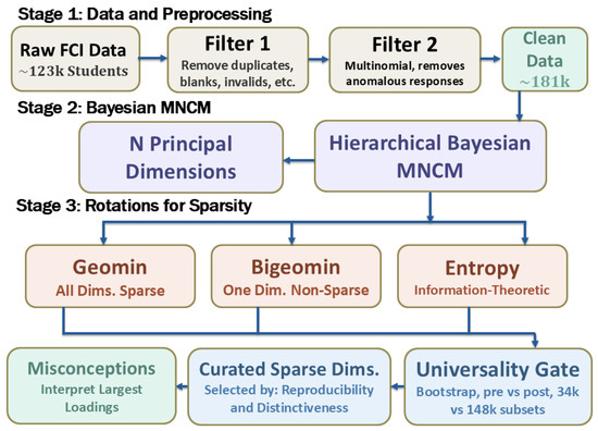
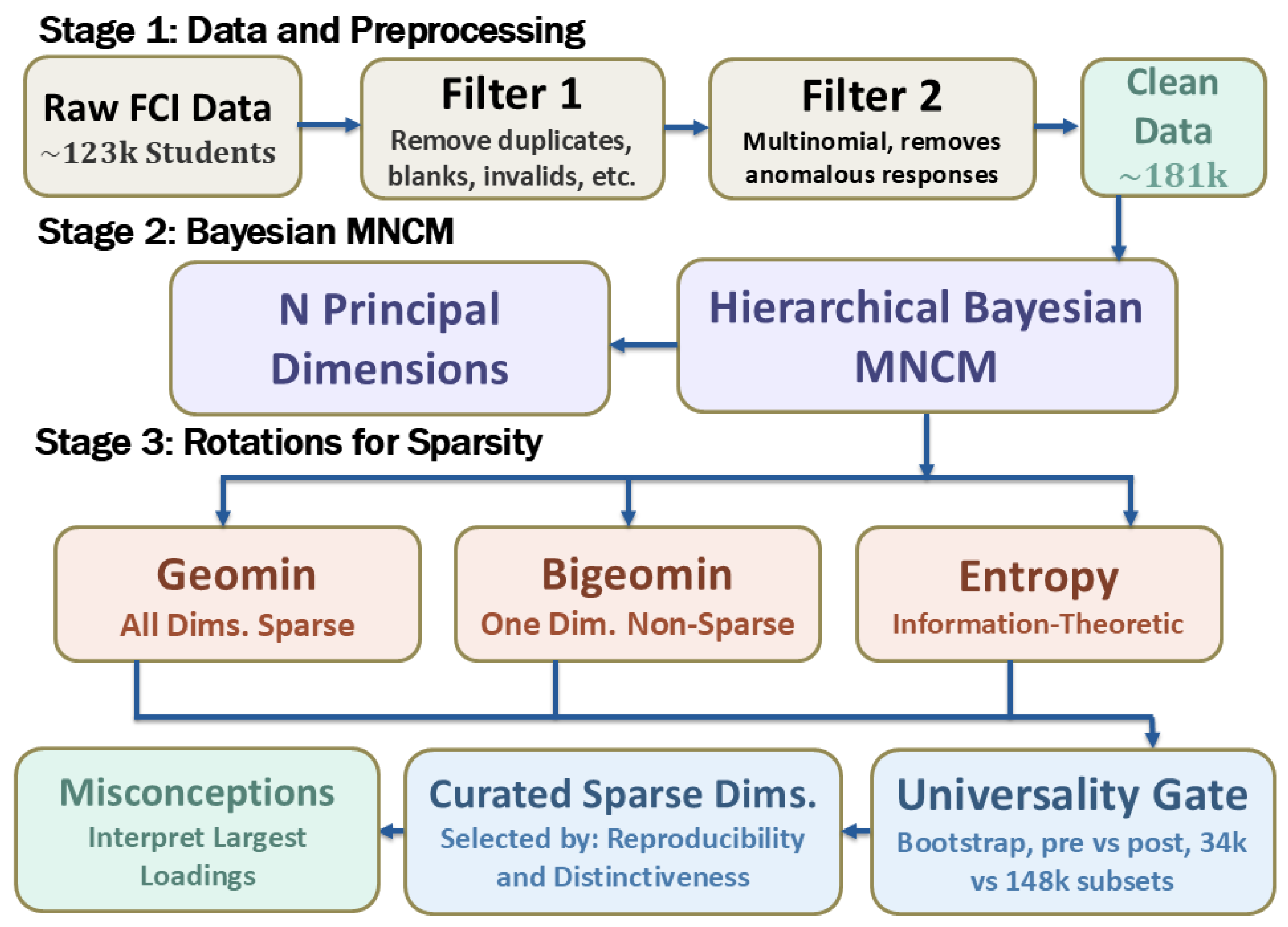
An overview of our full analytical pipeline is shown in Figure 1. It illustrates how raw response vectors are processed through cleaning, hierarchical Bayesian estimation, sparse rotation, and universality validation, ultimately leading to the identification of interpretable misconception dimensions. These developments are detailed in the following sections: in Section 2, we describe our collection of ∼204k responses from a concept test followed by a simple method to filter out responses from non-conscientious testees; in Section 3, the hierarchical Bayesian model for the multi-dimensional nominal categories model and its variational estimation is presented; and in Section 4, we present the rotation-based sparse representation, validate it across bootstrap and independent subsets, and demonstrate that these sparse vectors provide reliable inference in high-dimensional categorical data by connecting most of them with known misconceptions. In doing so, we contribute to the broader aims of this Special Issue by showcasing a valuable application of Bayesian hierarchical modeling and scalable inference that provides a meaningful interpretation for high-dimensional analyses of educational data. We also hope that our procedures will find application in other domains—including genomics, neuroscience, machine learning, and the social sciences, where researchers confront large datasets with complex dependence structures and latent variables whose dimensionality may itself be uncertain.

Figure 1. Overview of the analysis pipeline, from raw FCI data through filtering, hierarchical Bayesian MNCM estimation, sparse rotation, and universality validation to identified misconceptions.

2. Data and Preprocessing

We analyzed data from the 1995 revision of the Force Concept Inventory [1,9], a pioneering concept test designed to probe student understanding of the fundamental principles of Newtonian mechanics. The FCI consists of 30 multiple-choice questions, each with five response choices (categories), including one correct answer and several distractors intentionally designed to reflect common student misconceptions about force and motion. The results obtained with this instrument showed that most students finishing an introductory Newtonian mechanics course lacked the ability to consistently apply Newton’s laws to everyday circumstances and that standard lecture-based instruction improved their ability to do this by less than 25% [10]. Because of its diagnostic value, the FCI has become a central instrument in physics education research (PER) and has been used extensively to study instructional effectiveness, conceptual changes, and persistent misconceptions in introductory mechanics courses [10,11,12]. Student responses have therefore been collected by discipline-based organizations and research groups as part of efforts to measure and improve instruction. These data sources are described in Section 2.1 below, and the steps that we took to clean the data are described in Section 2.2.

2.1. Dataset Description and Origins

By combining the test results from numerous sources, several of which collected data from classrooms across a wide variety of schools, we obtained data from 203,564 administrations of the FCI, the vast majority of which came from pre- and post-instruction administrations by the teacher in charge of a particular college course. A smaller fraction originated from high-school implementations of the FCI and workshops involving pre-service or in-service teachers. The data from each administration constituted a response vector with a length of 30, where each component was A to E or some other symbol to indicate “no response” to that question.

2.2. Cleaning the Data: Identification and Removal of Problematic Response Vectors

Most large datasets, especially those like ours that are collected from multiple teachers at multiple schools, must be checked for errors and noise: duplicates, deliberate cheating by the subjects or others along the chain of collection, student use of heuristic test-taking strategies, signs of students running out of time, and responses by students who lacked the motivation or the honesty to enter data conscientiously. Most of these sources of error result in the student emphasizing or de-emphasizing some categorical responses or leaving blank responses.

To obtain a clean dataset suitable for analysis, we applied two filters. With Filter 1, we removed response vectors that were clearly duplicates, those containing any invalid responses (entries other than the valid answer choices A–E), and those with missing components (often indicated by *, “NA”, or “0”). These records were removed so that each remaining administration consisted only of valid responses to all 30 items. After applying Filter 1, the data had 191k usable FCI administrations (97,453 pre-instruction and 93,390 post-instruction tests), as detailed in Table 1.

Table 1. Summary of the FCI datasets used in this study and the sequential filtering steps applied to them. All counts are numbers of unique students. Raw lists the number of student records initially available from each dataset. Filter 1 retains administrations with complete pre- and post-test responses. Filter 2 applies a likelihood-based screen that removes administrations with anomalous distributions of answer choices across the 30 FCI items. The final columns report the mean pre-test score, mean post-test score, and normalized gain for each paired dataset. For further details on data provenance and access, see the Data Availability Statement.

Dataset	Subset	Raw	Filter 1		Multinomial		Mult. Removed (%)			Pre	Post	Norm.
			Pre	Post	Pre	Post	Pre	Post	Comb.			Gain
PhysPort	More Selective	22,551	12,452	17,864	11,866	10,942	4.7	38.7	24.8	13.80	18.49	0.29
	Selective	29,548	24,628	20,727	23,801	19,807	3.4	4.4	3.9	11.56	17.20	0.31
	Inclusive	12,034	8861	6934	8648	6923	2.4	0.2	1.4	12.88	17.14	0.25
	2 yr and Other	4629	3755	3299	3722	3279	0.9	0.6	0.8	13.57	17.39	0.23
	US High School	6935	5467	4764	5452	4753	0.3	0.2	0.3	9.19	17.06	0.38
	International	13,314	10,832	8592	10,785	8574	0.4	0.2	0.3	12.91	17.40	0.26
	Subtotal	89,011	65,995	62,180	64,274	54,278	2.6	12.7	7.5	12.28	17.47	0.28
LASSO		15,751	14,777	14,550	14,646	14,285	0.9	1.8	1.4	11.39	17.23	0.28
Modeling		10,039	8941	8941	8932	8940	0.1	0.0	0.1	8.09	16.32	0.39
Central Southwest		4363	4359	4359	4350	4358	0.2	0.0	0.1	12.29	21.43	0.52
Western Community College		195	193	190	193	190	0.0	0.0	0.0	13.55	20.55	0.47
Eastern Selective		165	71	71	71	71	0.0	0.0	0.0	20.77	26.66	0.59
AMTA		164	164	164	163	162	0.6	1.2	0.9	22.74	24.95	0.26
Eastern Private		159	150	132	150	132	0.0	0.0	0.0	8.23	12.39	0.19
Misc		3260	2803	2803	2801	2790	0.1	0.5	0.3	11.30	16.13	0.27
TOTAL		123,107	97,453	93,390	95,580	85,206	1.9	8.8	5.3	11.61	17.49	0.31

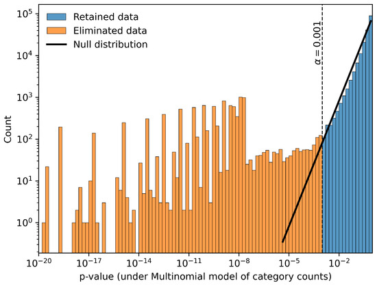
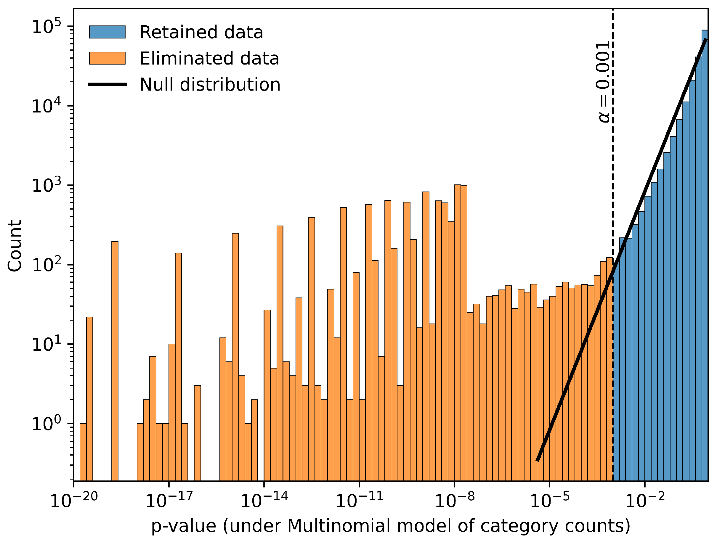
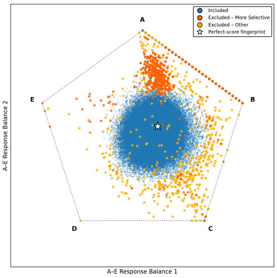
Filter 2 was designed to eliminate response vectors that had excesses or deficits of particular responses, which often resulted from heuristic test-taking strategies (e.g., always answer A or B when in doubt) or low-effort responding. This filter evaluated the probability of the “fingerprint” of each response vector (the number of responses of each category A, B, C, D, and E) according to a multinomial distribution based on the observed probabilities for each response from A to E in the retained data across the entire sample (see Figure 2). (The “observed probabilities” were determined after iteratively discarding outliers and re-fitting until reaching convergence.) The probability distribution for responses whose probability exceeded ${10}^{-3}$ was well-described by the null hypothesis—the assumption that deviations occur purely due to chance, a region spanning three orders of magnitude in probability. Consequently, these responses were retained. We estimated that this procedure may have discarded ∼300 legitimate responses and may have retained up 1k illegitimate responses. Prior work in our group using simulated data suggested that inducing 2% random answer changes does not significantly reduce the recovery of the original dimensions.

Figure 2. Distribution of response fingerprint p-values under a multinomial test. The solid line shows the expected distribution under the null hypothesis. Only those response vectors with p-values larger than 0.001 were retained. For better visibility of the retained bins, values smaller than ${10}^{-20}$ are not shown.

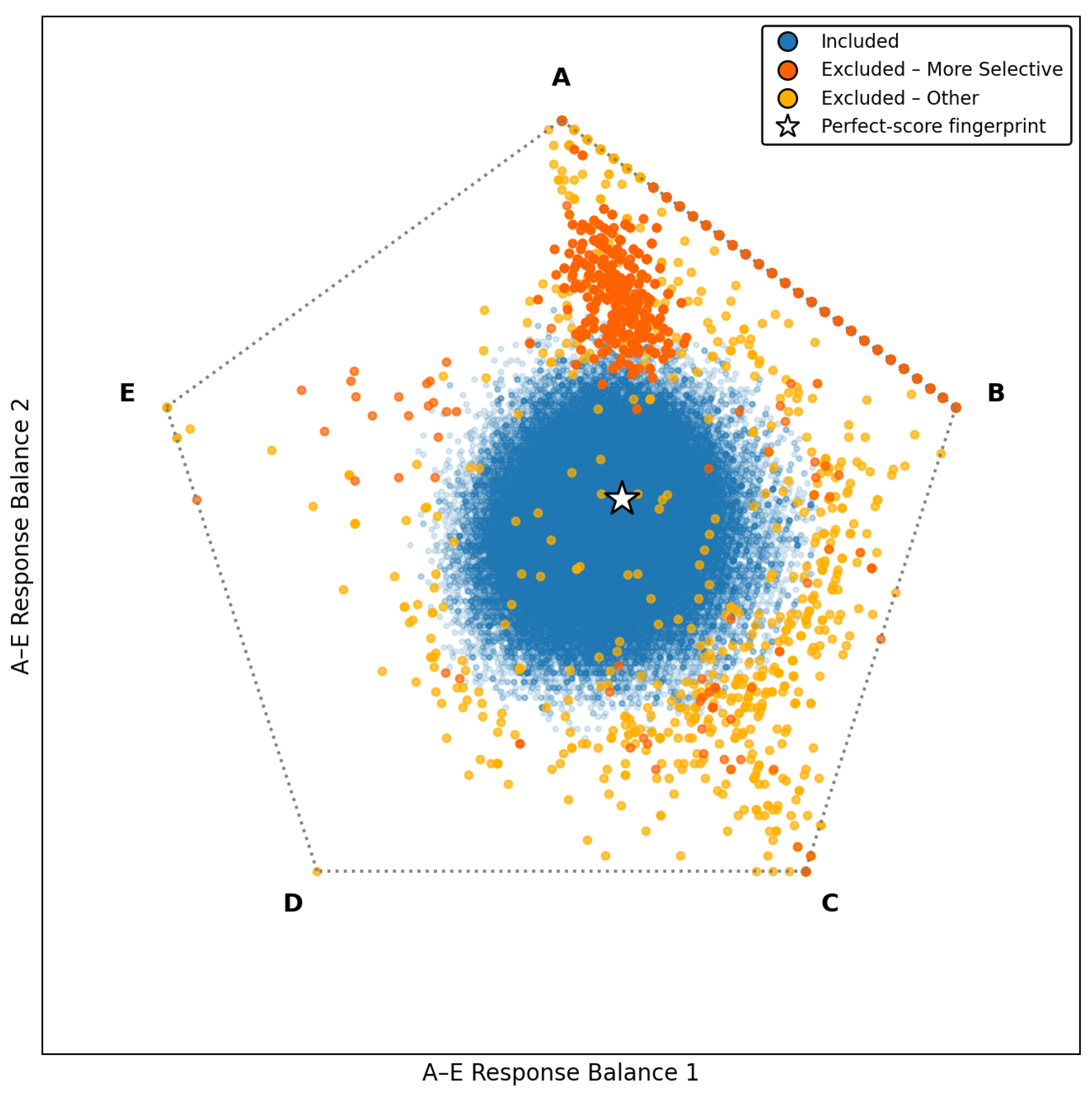
This procedure resulted in the elimination of ∼$1\%$ of the data for most of the datasets in Table 1, but $\sim 10\%$ for those colleges in the PhysPort data, concentrated in the post-test data from the “more selective” colleges. Almost 90% of all eliminated responses were due to students toggling randomly between A and B for every response, which accounts for the dotted line between the “all A” and “all B” vertices in Figure 3; these occurred almost exclusively in the “more selective” colleges and accounted for the response fingerprints with over 100 instances and a probability below $3\times {10}^{-8}$. Other excluded attempts followed the broader pattern of over-selection near vertices A and C seen across the full dataset.

Figure 3. Pentagon projection of response-vector balance scores for all test attempts. Each point represents one attempt mapped onto a two-dimensional pentagon basis, where vertices A–E correspond to the five answer choices. Blue points are retained attempts; dark orange points are attempts excluded from the more selective institutional subset; and yellow points are excluded attempts from all other groups. The white star marker indicates the perfect-score fingerprint.

In the remainder of the paper, we often analyze only a subset of the data in Table 1 above. The following table, Table 2, describes the particular subsets we used at different places:

Table 2. Summary of the major FCI datasets and derived data subsets used throughout this study. All reported sample sizes correspond to records that survived the preprocessing procedures described in Table 1 (Filters 1 and 2).

Size	Description
181k	All data after filtering.
34k	Old data from [13]; >50% high-school modeling classes.
148k	New data from Table 1, independent of 34k data; mostly PhysPort and LASSO, 80% intro college. Sometimes designated as 181k−34k to emphasize its independence from the 34k dataset.
96k	Pre-test data from 181k dataset.
85k	Post-test data from 181k dataset.
74k	Paired pre- and post-test data.

3. Bayesian Model Formulation and Inference

3.1. The Multi-Dimensional Nominal Categories Model

The category response curves (probability of selecting each category vs. raw overall score) provide strong evidence that students select categories on the FCI due to prior beliefs. If students whose raw score is near or below the score ($n_{correct}=6$) were randomly guessing, their CRCs would converge near the chance response ($p_c=0.2$). Instead, an examination of all of our pre-test CRCs showed that just over 1/2 of the questions had one distractor whose CRC approached $0.5$ or more as the raw score approached 0, dominating all other response categories. In addition, half of the questions had CRCs with maxima at intermediate raw score values. These facts are further evidence that students are not guessing on the FCI. The observed structure can only be fitted by a model that allows each distractor to have its own parameters [14]. Finding multiple dimensions, each of which represents the distractor selection pattern associated with a particular misconception, motivated us to select the multi-dimensional nominal categories model (MNCM; [15,16]), which generalizes Bock’s one-dimensional nominal categories model ([17]) to D latent dimensions. In the MNCM, the ability of student s on dimension d is denoted by ${\theta }_s^{\left(d\right)}$, and each dimension d loads on each item–category pair with slope $a_d^{(i,c)}$ to give a category “tendency”:

$$t_s^{(i,c)}=\sum _d{a}_d^{(i,c)}{\theta }_s^{\left(d\right)}+b^{(i,c)},$$

(1)

where each item–category pair also has an intercept parameter $b^{(i,c)}$, which allows the baseline response probabilities to differ across categories. The predicted probability that student s selects category c for item i is then given by the multinomial logistic function

$$p\left(r^{\left(i\right)}=c\mid {\mathbf{t}}_s^{\left(i\right)}\right)={\displaystyle \frac{exp\left(t_s^{(i,c)}\right)}{{\sum }_{c^{\prime }}exp\left(t_s^{(i,c^{\prime })}\right)}}.$$

(2)

Although the symmetric form of Equation (2) treats all categories even-handedly during inference, applying the simple constraints described below (setting $a_d^{(i,c_i^{*})}=0$ and $b^{(i,c_i^{*})}=0$ for all d in post-processing) yielded results that were equivalent to reference–category parameterization. After this step, the probability that student s selects distractor $k\ne c_i^{*}$ takes the form

$$p\left(r^{\left(i\right)}=k|{\mathbf{t}}_s^{\left(i\right)}\right)={\displaystyle \frac{exp\left(t_s^{(i,k)}\right)}{{\displaystyle 1+\sum _{c^{\prime }\ne c_i^{*}}exp\left(t_s^{(i,c^{\prime })}\right)}}},k\ne c_i^{*},$$

(3)

and the probability of a correct response is simply

$$p\left(r^{\left(i\right)}=c_i^{*}|{\mathbf{t}}_s^{\left(i\right)}\right)=1-\sum _{k\ne c_i^{*}}p\left(r^{\left(i\right)}=k|{\mathbf{t}}_s^{\left(i\right)}\right).$$

(4)

These expressions are presented only to show the connection to the reference–category logistic form; the data are fit using the original symmetric form (2), with the identification constraints imposed analytically later in the processing.

This model is used in several fields and is also known as the multi-dimensional nominal response model (MNRM) [18], nominal factor analysis [19], multi-dimensional generalization of the nominal categories model [20], and MAXMC [21]. The formulation is mathematically equivalent to a multinomial logistic regression with D latent predictors.

Combining the response tendencies across all items and categories into matrix notation allows for a more compact representation. Let

• $\mathit{T}\in {\mathbb{R}}^{S\times IC}$ denote the matrix of student response tendencies, where each row corresponds to a student s and each column to an item–category pair $(i,c)$;
• $\mathbf{\Theta }\in {\mathbb{R}}^{S\times D}$ denote the matrix of student latent ability vectors, where each row corresponds to a student s and each column to a latent dimension d;
• $\mathbf{A}\in {\mathbb{R}}^{D\times IC}$ denote the matrix of category slope vectors across all items and categories;
• $\mathbf{b}\in {\mathbb{R}}^{1\times IC}$ denote the vector of category intercepts.

(Note that, in this notation, dimensions are associated with rows of $\mathbf{A}$ rather than columns).

For reference, Table 3 summarizes the key symbols used in this paper, grouped by their level in the model hierarchy.

Table 3. Summary of model notation grouped by level in the hierarchy.

Symbol	Meaning	Level
${\theta }_s^{\left(d\right)}$	Latent ability of student s on dimension d	Student
$\mathbf{\Theta }\in {\mathbb{R}}^{S\times D}$	Full matrix of student ability vectors	Student
$a_d^{(i,c)}$	Slope of item–category $(i,c)$ on dimension d	Item
$\mathbf{A}\in {\mathbb{R}}^{D\times IC}$	Full matrix of slope vectors	Item
$b^{(i,c)}$	Intercept for item–category $(i,c)$	Item
$\mathbf{b}\in {\mathbb{R}}^{1\times IC}$	Full vector of intercepts	Item
${\alpha }_d$	Scale hyperparameter for prior SD of slopes on dim. d	Hyperparameter
$\beta$	Scale hyperparameter for prior SD of intercepts	Hyperparameter

The MNCM is subject to multiple classes of indeterminacy: location invariance of the abilities, location invariance of the item parameters, scale invariance, and rotation invariance. These invariances require additional care to address compared to a fully identified model, but also allow for transformations that yield more interpretable results.

In the first case, shifting all student abilities on any dimension d leaves the predicted response probabilities unchanged, provided the intercepts are adjusted accordingly. We resolved this by centering $\mathbf{\Theta }$ at zero across the student sample for every dimension, compensating with the following adjustment to the intercepts:

$$\Delta b^{(i,c)}=\sum _d{a}_d^{(i,c)}{⟨{\theta }^{\left(d\right)}⟩}_s,$$

(5)

where ${⟨·⟩}_s$ represents the arithmetic mean over students.

In the second case, an examination of the model formulation will reveal that the slope and intercept parameters for each item are partly redundant: all may be shifted (independently per item, and per dimension for the slopes) by the same additive constant without changing the probabilities. To eliminate these shift invariances, two traditional approaches exist: simple constraints (fixing the slope and intercept of a clear reference category to zero where one exists, such as for the keyed correct-answer category) or deviation constraints (centering category parameters within each item such that ${⟨a_d^{(i,c)}⟩}_c=0$ and ${⟨b^{(i,c)}⟩}_c=0$). We applied simple constraints for ease of interpretation, yielding slope and intercept parameters for the distractors whose values may be understood relative to the correct answer in each item.

Finally, any invertible linear transformation applied to $\mathbf{\Theta }$ (with the corresponding inverse transformation applied to $\mathbf{A}$) also preserves the predicted response probabilities. This combined scale-and-rotation freedom was initially resolved by constraining the sample covariance matrices of $\mathbf{\Theta }$ and $\mathbf{A}$ to be the identity matrix and diagonal matrix, respectively, and by ranking dimensions in order of decreasing slope variance.

The scale-and-rotation indeterminacy and the student ability centering were softly regularized during model fitting via the Bayesian prior (see Section 3.2), with exact constraints applied analytically as a post-processing step ([2]).

3.2. Bayesian Hierarchical Modeling

We embedded the MNCM in a hierarchical Bayesian framework as suggested by [6]. Global scale hyperparameters ${\alpha }_d$ and $\beta$ govern the prior standard deviations of item slopes and intercepts, respectively, allowing the data to determine the effective strength of each latent dimension. The full generative model (6)–(9) uses a weakly informative half-Cauchy hyperprior for these parameters. This distribution has wider tails than a normal distribution—allowing the model to accommodate strongly discriminating dimensions if warranted—while its non-vanishing density near the origin allows unnecessary dimensions to be shrunk toward zero, acting as a soft regularizer on model dimensionality.

$$\begin{array}{cc}\hfill {\alpha }_d,\beta & \sim \mathrm{HalfCauchy}\left(5\right),\hfill \end{array}$$

(6)

$$\begin{array}{cc}\hfill a_d^{(i,c)}& \sim \mathcal{N}(0,{\alpha }_d),\hfill \end{array}$$

(7)

$$\begin{array}{cc}\hfill b^{(i,c)}& \sim \mathcal{N}(0,\beta ),\hfill \end{array}$$

(8)

$$\begin{array}{cc}\hfill {\theta }_s^{\left(d\right)}& \sim \mathcal{N}(0,1).\hfill \end{array}$$

(9)

The prior means of all item parameters were fixed at zero (the invariances in the model made this choice arbitrary), and student abilities ${\theta }^{\left(d\right)}$ were assigned standard normal priors consistent with conventional IRT practice.

The scale parameter $\tau =5$ in Equation (6) was chosen to be weakly informative relative to typical IRT discrimination parameters. In standard IRT practice, slope values above 3 are already considered high [22], so $\mathrm{HalfCauchy}\left(5\right)$ assigns substantial probability to the range $[0,5]$ while retaining heavy tails that permit larger values when warranted by the data, and a non-negligible density near zero that allows unnecessary dimensions to be effectively shrunk out. This choice follows the recommendation of [6] for weakly informative half-Cauchy priors in hierarchical IRT models.

Bayesian inference requires solving Bayes’ law for the posterior distribution over all latent variables, $\Omega =\{\mathbf{\Theta },\mathbf{A},\mathbf{b},\mathbf{\alpha },\beta \}$, given the observed responses R:

$$p(\Omega \mid R)={\displaystyle \frac{p(R\mid \Omega )p(\Omega )}{p\left(R\right)}}.$$

(10)

Unfortunately, this is analytically intractable. Markov chain Monte Carlo (MCMC) is a common approximation method, but it is computationally expensive. Instead of MCMC, we adopted stochastic variational inference (SVI; [23]), which reformulates the posterior inference as an optimization problem. Rather than computing the posterior directly, SVI fits an analytically tractable approximation to the posterior distribution, $q(\Omega )\approx p(\Omega )$, by maximizing a surrogate objective called the evidence lower bound (ELBO; [24]).

Our choice of $q(\Omega )$ followed a mean-field normal approximation. Formally, the variational distribution factorized completely across all latent variables,

$$q(\Omega )=\prod _{\omega }{q}_{\omega }\left(\omega \right),$$

(11)

where each marginal factor $q_{\omega }$ is a univariate Gaussian $\mathcal{N}({\mu }_{\omega },{\sigma }_{\omega }^2)$ for real-valued variables (slopes, intercepts, and student abilities), or a Gaussian mapped through the softplus transform $x\mapsto log(1+e^x)$ for positive-constrained variables (${\alpha }_d$, $\beta$, and all posterior standard deviations). The parameters $\{{\mu }_{\omega },{\sigma }_{\omega }\}$ across all latent variables constitute the variational parameters, jointly optimized to maximize the ELBO. The mean-field Gaussian family is the standard choice for large-scale Bayesian inference because it yields tractable ELBO gradients computable via the reparameterization trick.

A known limitation of the mean-field approximation is that the factorized structure cannot represent posterior correlations among parameters, leading to the underestimation of marginal posterior variances. In practice, this primarily affects the calibration of the posterior standard deviations rather than the posterior means—the expected a posteriori (EAP) values that are used in all downstream analyses in this paper. We address this empirically in Section 4.2: by re-running Bayesian inference on 50 independent bootstrap resamples of the data, we characterized the overall end-to-end variability in the sparse dimensions without relying on the variational posterior variances.

Optimization proceeded via the Adam optimizer [25]. The training loss (ELBO) was monitored throughout optimization; after a set number of iterations, the learning rate was reduced according to a cosine schedule to refine the search for the global minimum. Parameter initialization followed an adaptation of the fast IRT approximation described by [26] to improve the convergence speed. The final point estimates were obtained as EAP values extracted from the fitted variational distributions.

4. Interpreting Latent Dimensions: Rotations and Misconceptions

A central problem with procedures that extract multiple dimensions or factors (as with exploratory factor analyses) from large datasets is interpreting the results so that they are understandable and informative. In fact, this problem was our motivation for our research agenda: we wanted to discover and study student misconceptions using a large sample of response vectors from the FCI, with the ultimate objective of developing specific remedial pedagogies. These desires motivated our selection of the MNCM and the development of the methods described in this paper (and [2])—all based on the expectation that our hypothesis would be verified that misconceptions would manifest as a small set of wrong answers (“distractors”) on the FCI (or any other research-designed concept test) that would be preferentially selected by students harboring that misconception. Since the distractors on the FCI cover numerous misconceptions, we expected that a single misconception would “load” on only a few distractors. This was achieved by rotating the principal vectors found by the MNCM to obtain sparse dimensions that load heavily on just a few distractors.

In this section, we first identify a curated set of sparse dimensions from multiple rotated solutions, then demonstrate that they are highly universal, i.e., invariant across various subsamples of our data (including those with different instructional levels and demographic compositions). We show that most of these can be identified as misconceptions (or special cases of them), mostly known from the prior misconceptions literature.

4.1. Rotations Find Sparse Dimensions

The principal dimensions discovered by the hierarchical Bayesian procedures described above typically load significantly on many distractors across multiple questions and therefore are not interpretable as a single misconception. The key to finding sparse dimensions is to transform these principal dimensions so that each transformed dimension loads heavily on only a few distractors, thus facilitating their interpretation. This is allowed because the tendencies (Equation (1)) that predict the probabilities of a student’s responses are invariant under the joint rotation of both the student ability vectors and the loading vectors ($\theta$ and a), since the corresponding tendencies are proportional to the scalar product of $\theta$ and a. This general result, exploited in standard factor analyses, is apparent when looking at the tendency equation in matrix form:

$$\mathit{T}=\mathbf{\Theta }\mathit{A}+\mathit{b}=\mathbf{\Theta }\left(\mathit{R}{\mathit{R}}^{-1}\right)\mathit{A}+\mathit{b}=\left(\mathbf{\Theta }\mathit{R}\right)\left({\mathit{R}}^{-1}\mathit{A}\right)+\mathit{b}$$

(12)

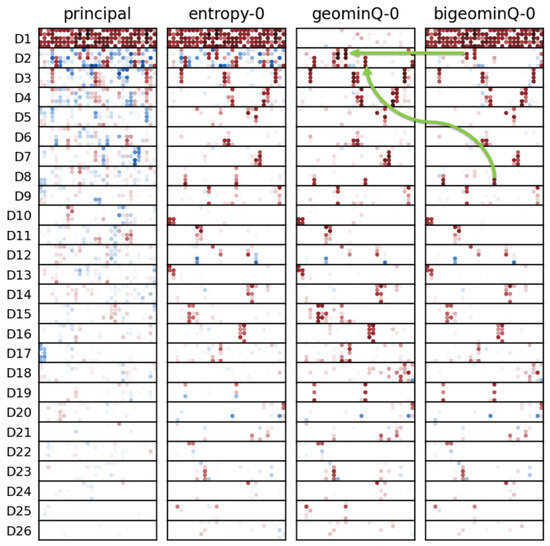
Our group’s exploration of rotation methods to find sparse vectors [13] explored roughly a dozen to find those that produce the most universal dimensions that clearly correspond to one (or two) intellectually consistent misconceptions. Here, we limited ourselves to the most promising transformation method in each of three major categories: an orthogonal method (the minimum-entropy rotation, which has its basis in information theory), an oblique method (geominQ), and an oblique bi-factor method (bigeominQ), which explicitly permits a single non-sparse dimension. Each of these was applied 100 times with random initial rotation matrices in order to fully explore the solution space, which generally contained several informative local minima of the rotation criterion. The best minimum found was designated by the suffix “-0”, as shown in Figure 4. Due to the rotation invariance of the MNCM, the ordering of the sparse dimensions is somewhat arbitrary—we attempted to match these as closely as possible in this figure for ease of comparison.

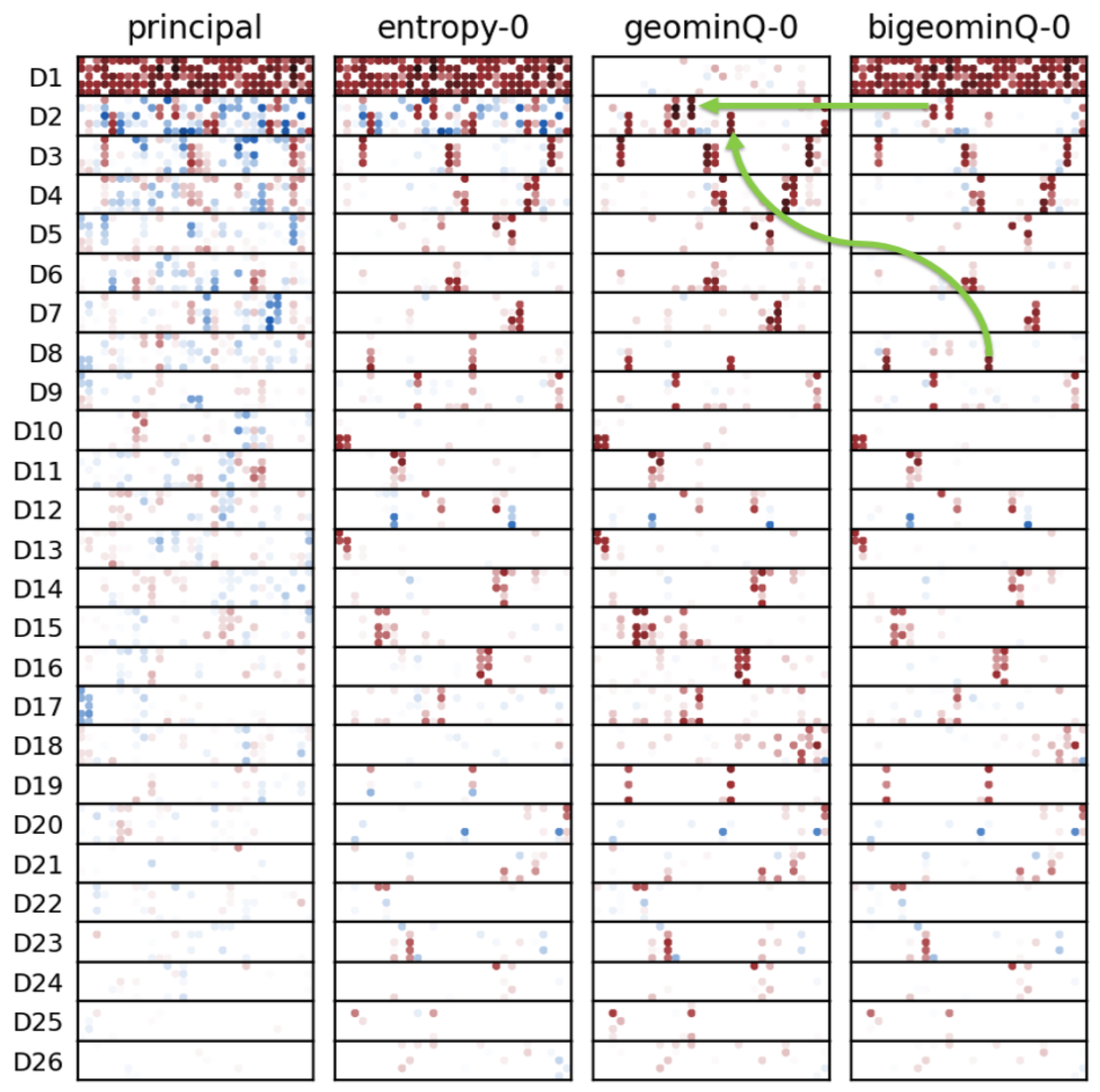
Figure 4. Principal and selected Sparse Rotations. Each small rectangular panel depicts the loadings in a specific dimension as a grid of dots (red for negative and blue for positive) indexed horizontally by item (1–30) and vertically by category (A–E). Note that dimensions 3–26 of both types of sparse rotations as well as entropy are highly similar, showing the invariance of the sparse dimensions across different types of transformations. The green arrows highlight how D2 and D8 of bigeomin combine to give D2 of geomin; note that this pattern also appears in the other second dimensions.

The first principal dimension loaded negatively on every distractor, clearly identifying it as “Newtonian incorrect”. Functionally-identical versions of this dimension were also found by two of our three factor rotation methods; its dominance confirmed that the FCI is, indeed, primarily a test of Newtonian beliefs about force and motion. The subsequent principal dimensions were considerably weaker, especially those in higher dimensions, and generally loaded on many distractors that were not readily interpretable.

We were surprised by both the large fraction of shared sparse dimensions and their high degree of similarity (obvious in Figure 4) across the entropy, geomin, and bigeomin rotations. This is a testament to the invariance of the fundamental structure of the underlying data, since these rotations use substantially different methods to achieve sparseness. In cases where these best-matched dimensions did differ substantially, the alternate version was sometimes found in the local-optimum solutions of the other rotation methods. For example, D2 of geomin combines dimensions D2 and D8 of bigeomin; this combination was also prominent in entropy.

From the various local solutions found by our different rotations, we selected a subset of curated sparse dimensions, emphasizing those that appeared consistently across different methods and initializations, that were supported by a small bootstrap reproducibility study (described below), that were preferentially from bigeominQ-0, and/or whose set of prominent distractors corresponded to an interpretable intellectual construct. Since we drew from multiple local solutions (an approach inspired by [27]), we found three more curated sparse dimensions than principal dimensions; we noted that the curated dimensions were therefore not all linearly independent, but in some instances represented several different (and equally valid) ways of interpreting the same data.

The set of 29 curated dimensions along with their associated statistics is tabulated in Table 4. The majority of these correlate highly with misconception dimensions obtained from a smaller ∼34k-administration dataset [13]; for consistency, we named these using the same roman numerals as in that work, and also provide a textual description of each matched misconception based on our earlier work. For the two dimensions that lacked an obvious “anti-Newtonian” sign convention (XI and XVIII), we additionally retained the same (arbitrary) sign convention as used in our previous work. Note that several roman numerals are missing; they were removed for reasons discussed in [13].

Table 4. Curated sparse dimensions. For each, we indicate the rotated solution set from which it was taken as well as the dimension number within that set (cf. Figure 4), the median bootstrap correlations in the complete dataset as well as in the pre- and post-test only subsets, and the sum of within-item variances in the dimension’s $a^{(i,c)}$ parameters (which provide a rough overall measure of the overall strength). For dimensions closely matching those found in our earlier work [13], we adopted the same roman-numeral designations and also noted what physics misconception they appeared to be encoding. We further illustrate the stability of these re-discovered results by providing uncentered correlation coefficients between the earlier dimensions (found from a much smaller dataset of ∼34k administrations) and those obtained from a completely independent (non-overlapping) subset of our current data.

		${\mathit{r}}_{\mathbf{bootstrap}}$
Name	Source	All	Pre	Post	$\mathbf{\sum }\mathbf{Var}$	Description	${\mathit{r}}_{\mathbf{34}\mathbf{k}\mathbf{–}\mathbf{148}\mathbf{k}}$
I	bgQ-0 D1	1.00	0.99	0.98	23.8	Newtonian incorrect	0.99
II	bgQ-0 D4	1.00	0.98	0.98	2.6	Applied force exceeds resistance for constant speed	0.97
III	bgQ-0 D8	0.99	0.94	0.96	2.5	Impetus force, mostly on circular path	0.94
IV	bgQ-2 D8	0.99	0.91	0.94	1.1	Impetus plus centrifugal or centripetal force on circular path	0.93
V	bgQ-0 D3	1.00	0.98	0.98	2.4	Active dominates massive, which dominates passive	0.98
VI	bgQ-0 D2	0.99	0.94	0.94	2.1	Impetus force, mostly along linear path	0.93
VII	bgQ-2 D2	1.00	0.98	0.98	3.6	Impetus force on both linear and circular paths	0.98
VIII	bgQ-0 D6	0.99	0.97	0.70	1.2	Passive object pushed “because in the way”	0.92
IX	bgQ-0 D5	0.99	0.98	0.96	1.3	After rocket starts or stops, goes in direction of latest force or earlier motion	0.96
X	bgQ-0 D9	0.99	0.97	0.70	1.1	Omission of reaction force (normal or from passive object), usually with gravity	0.94
XI	bgQ-0 D12	0.99	0.94	0.94	1.1	Straight path preferred vs. curved paths	0.86
XIII	bgQ-0 D7	0.99	0.98	0.96	1.0	Decelerating after impulse from rocket firing	0.96
XIV	bgQ-0 D13	0.99	0.96	0.93	0.9	2M and M balls differ by factor of 2	0.88
XV	bgQ-0 D11	0.99	0.98	0.96	1.0	Latest force dominates after sudden force	0.93
XVI	bgQ-0 D21	0.98	0.86	0.90	0.7	Force change increases speed to a constant speed (not forever)	0.89
XVII	bgQ-1 D22	0.98	0.89	0.95	0.7	Continues curving inwards after inward force removed	0.92
XVIII	bgQ-0 D20	0.99	0.93	0.89	0.7	Air exerts significant drag and downward force	0.92
XIX	bgQ-0 D14	0.99	0.95	0.94	0.9	No acceleration due to rocket firing	0.87
XXI	bgQ-0 D10	0.99	0.97	0.95	1.1	2M ball falls significantly faster, but not by factor of 2	0.93
XXIII	bgQ-0 D19	0.98	0.93	0.91	0.9	Missing centripetal force	0.90
XXVI	bgQ-0 D16	0.99	0.97	0.91	0.6	Motion diagrams; v and a confused	0.94
XXVII	bgQ-0 D25	0.97	0.91	0.80	0.4	Gravity stronger when closer to ground	0.81
XXVIII	bgQ-0 D15	0.98	0.91	0.92	0.6	–	–
XXIX	bgQ-0 D22	0.97	0.85	0.79	0.7	–	–
XXX	bgQ-1 D15	0.96	0.87	0.68	0.5	–	–
XXXI	bgQ-0 D24	0.97	0.90	0.81	0.5	–	–
XXXII	bgQ-0 D18	0.98	0.93	0.81	0.9	–	–
XXXIII	bgQ-0 D17	0.97	0.90	0.83	0.7	–	–
XXXIV	bgQ-0 D23	0.98	0.94	0.85	0.6	–	–

4.2. Sparse Dimensions Are Universal Patterns

We now demonstrate the universality of our results by showing their high degree of invariance across various subsets of the data, including:

• Random resamples of our complete dataset (via non-parametric bootstrapping)
• Administrations before and after instruction
• Mostly high-school students (our earlier 34k-administration dataset with >50% high-school students) vs. mostly college students (the 181k–34k dataset excludes the earlier 34k dataset and comprises over 80% college students).

4.2.1. Non-Parametric Bootstrap

As a first measure of the overall reproducibility, we conducted a small bootstrap study by randomly generating 50 full-size bootstrap resamples of our 181k dataset, with sampling stratified to maintain a consistent ratio of pre- and post-test data. We ran our full hierarchical Bayesian analysis on all such resamples, as well as on the pre-test-only and post-test-only subsets of each, resulting in 150 sets of principal dimensions after inference. Each of our curated dimensions was then compared to the bootstrapped sets of principal dimensions using a form of a Procrustes analysis: each principal solution was rotated obliquely to maximize the correlation coefficient with the curated dimension in question, and this “best-aligned” correlation was recorded. Recognizing that such a procedure would yield inflated correlations (as even random matrix results will yield substantial correlations when rotated to maximize the alignment in a 26-dimensional space), we also computed random-chance baseline correlations using a permutation method, using these to linearly deflate each Procrustes-rotated bootstrap correlation ($r_{\mathrm{adjusted}}=[r_{\mathrm{original}}-r_{\mathrm{chance}}]/[1-r_{\mathrm{chance}}]$). These results are reported in Table 4.

Even after adjusting for chance, the median correlations for the full-size bootstrap resamples were extremely high: the minimum adjusted value across all curated dimensions was 0.96, with most being 0.99 or greater. Those comparing the curated dimensions to pre- and post-only resample results were necessarily lower, since cutting the size of the data by half leads to fewer dimensions being recovered during inference. Nevertheless, the majority remained high on at least one of the pre- or post-test results, with only two of our newly-identified dimensions (XXIX and XXX) falling below 90% on both. Overall, these results provide evidence that our sparse dimensions are quite invariant across student samples, with most also demonstrating invariance across pre- and post-testing.

4.2.2. Invariance of Sparse Dimensions Extracted from Pre- and Post-Test Data

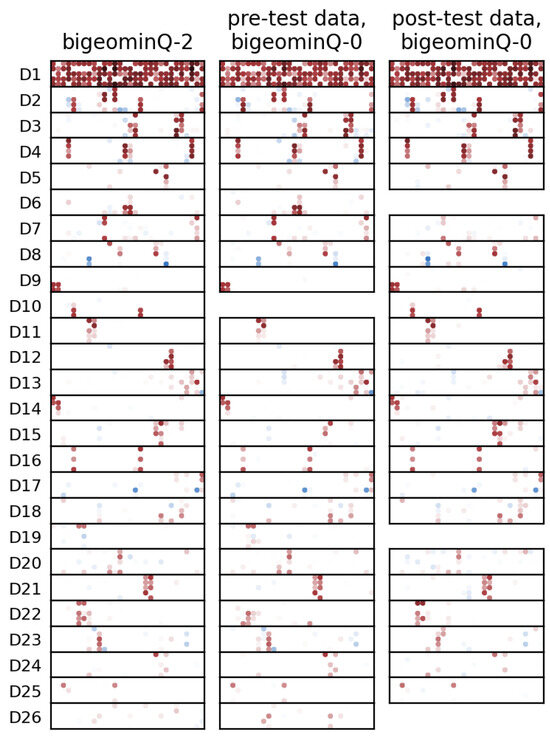
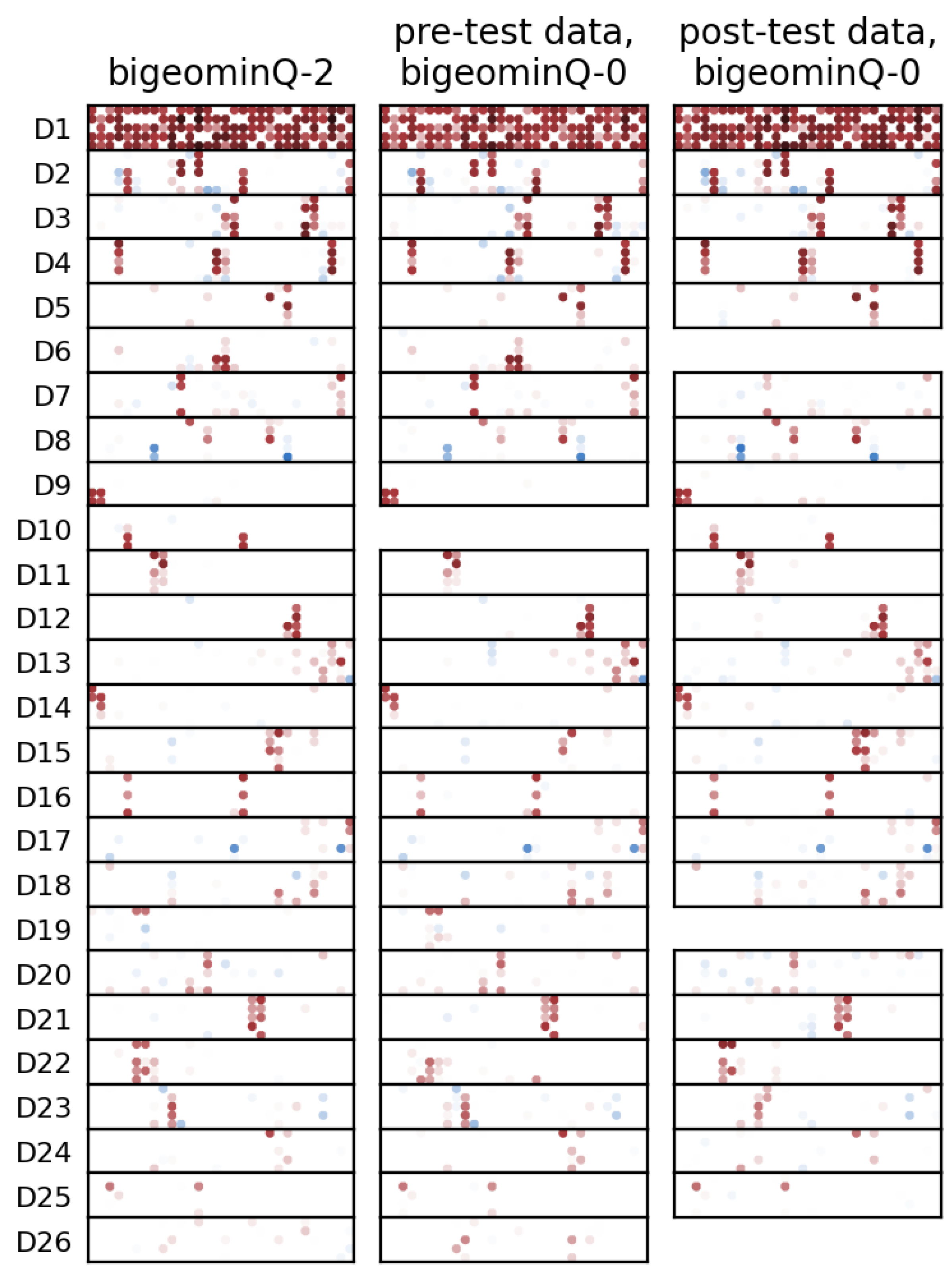
In addition to the adjusted bootstrap correlations above, we explored the degree of similarity between sparse solutions obtained separately from the pre- and post-test data. These solutions were computed using the same methodology as our full-data results: the application of the hierarchical Bayesian MNCM, followed by rotation with several methods from 100 random initializations. We chose the best solutions obtained by the oblique bigeomin method (i.e., bigeominQ-0) in both cases, and present these results side by side in Figure 5. For comparison, we also include a bigeomin solution for the complete data; here, we used one of our prominent local optima (bigeominQ-2), as this corresponded better to the solutions shown for the pre- and post-test solutions.

Figure 5. Sparse dimensions on all data, only pre-test data, and only post-test data. The dimensions are notably similar. Gaps in the pre- and post-test columns indicate that no similar pattern was found because the variance in that dimension did not rise above the noise in these smaller datasets. Blue and red dots indicate postive and negative loadings respectively (see Figure 4 caption).

Clearly, an entire semester (or quarter) of Newtonian physics instruction does not significantly change the nature of nearly all sparse dimensions. Of course, the extent to which each underlying misconception is held by a class of students will (hopefully) be reduced by instruction; this will be discussed in future work.

Despite the overall similarity, there are some notable differences between the three sets of results shown. First, the pre- and post-test analyses recovered fewer overall dimensions, with D10 missing in the pre-test results and D6, D19, and D26 missing in the post-test results. This does not on its own indicate that these dimensions are entirely absent in the true generating model for these datasets; however, it does suggest that they are weak enough to be below the threshold of detectability given the smaller sample sizes and (likely) differing variance in the associated student traits across these datasets. Second, a small subset of dimensions were present, but substantially altered, in one of the solutions (e.g., D15 and D22 for the pre-test, D13 and D23 for the post-test). Further study is needed to determine whether these differences correspond to actual changes in students’ underlying conceptual models or whether they are merely due to the sensitivity of the rotation minima to small perturbations of the loadings in such a high-dimensional space.

4.2.3. Invariance of Sparse Dimensions Extracted from High-School and College Students

As a final test, we compared sparse dimensions obtained from two non-overlapping subsets of our data with qualitatively different student demographics. The first of these subsets contained ∼34k administrations of the FCI, with more than half of these coming from high-school students taught by teachers who had taken the modeling instruction workshop run by D. Hestenes’ group at Arizona State University. Sparse dimensions found using these data were reported in previous work by our group [13], where they were found to correspond to identifiable misconceptions in physics known from the PER literature and teacher experience.

The second subset contained only administrations that were not present in the original 34k dataset; it contained 148,473 administrations and consisted primarily of the PhysPort and LASSO datasets in Table 1. Over 80% of these data were obtained from introductory college students who were taught with a variety of pedagogies, but rarely with modeling pedagogy.

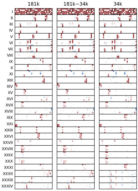
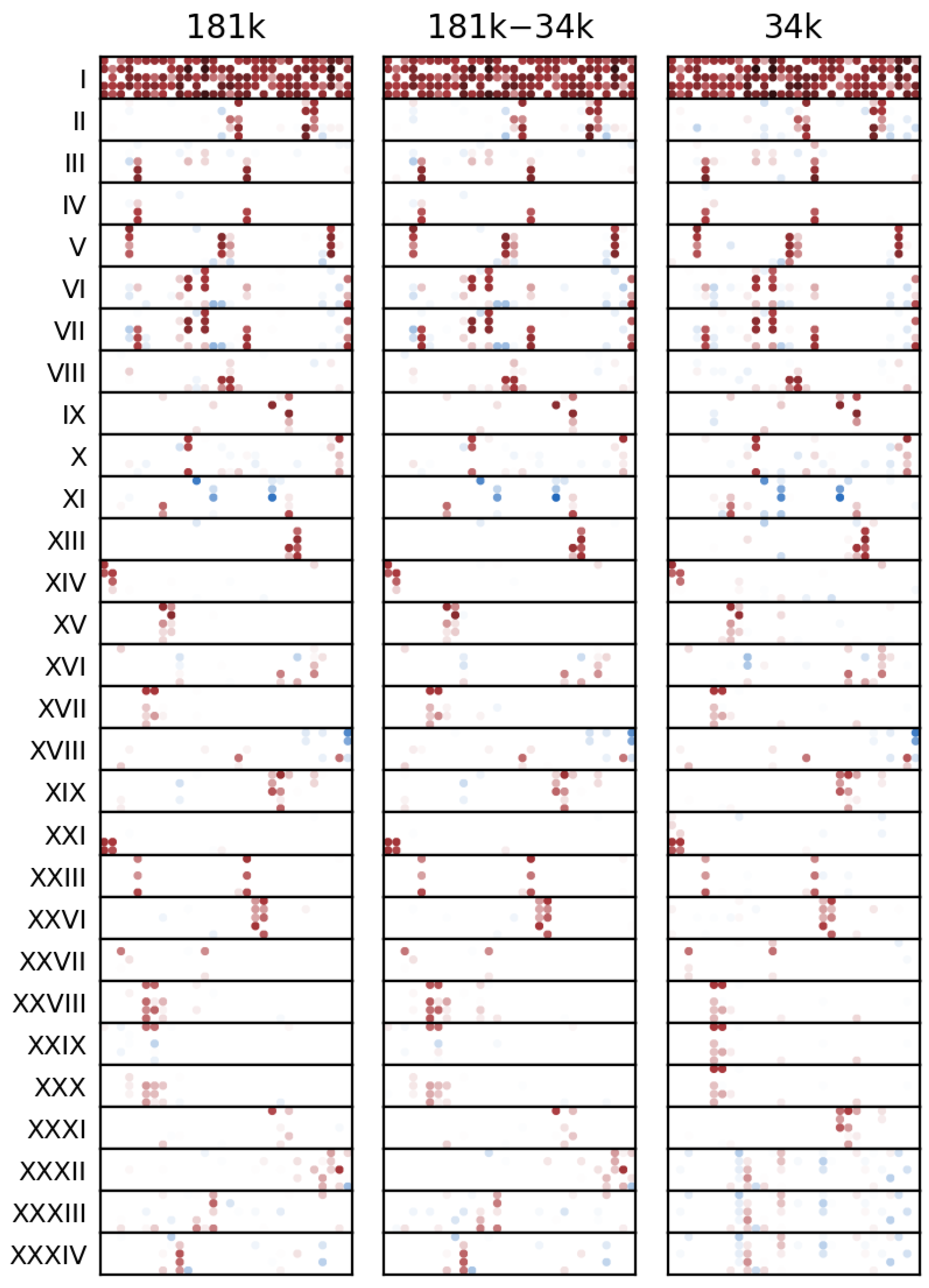
The high degree of similarity between the “misconception dimensions” from our earlier study and the sparse dimensions obtained from non-overlapping data in the present work is immediately apparent in Figure 6. We quantified this similarity between the old dimensions and their closest analogs in the new results using the uncentered Pearson correlation of the loadings, and include these values in the right-most column of Table 4 (labeled “$r_{34\mathrm{k}–148\mathrm{k}}$”). All but four correlations were greater than 0.9, and none were below 0.8. The fact that so many of these sparse dimensions were so similar despite substantial differences in the demographics of the students from whose responses they were discovered is a very encouraging finding.

Figure 6. Curated sparse dimensions (left column) from our 181k dataset alongside similar dimensions obtained from two smaller datasets. The results labeled “34k” (right column; previously reported by [13]) comprise over 50% high-school administrations and are completely independent of those in the center column (labeled “181k–34k”), which are over 80% college students. Both large datasets bear strong similarity to dimensions in our earlier work, with more dimensions discoverable and higher dimensions clearer in the larger datasets. Blue and red dots indicate postive and negative loadings respectively (see Figure 4 caption).

Figure 6 also includes one 34k dimension that we discarded in our earlier results as an uninterpretable residual (shown in the lower three panes of the right-most column). We observed that our larger dataset appears to resolve this into three distinct dimensions, all of which are simpler and—in our view—far more likely to admit meaningful interpretations.

4.3. Most Curated Sparse Dimensions Are Misconceptions

Where possible, it is valuable to identify our sparse dimensions as specific misconceptions for three main reasons:

• It shows that these dimensions meet the definition of a stable mental misconception, thereby confirming the fundamental hypothesis of this paper;
• It demonstrates the value of applying hierarchical Bayesian analysis methods in education;
• It provides a list of validated “misconception dimensions” as a basis for future education-relevant work by us and others, and especially for those studying the FCI for whom replicating the full inference pipeline is not practical.

As described above, most of our dimensions were already found to correspond to new or established misconceptions in earlier work, and a cursory examination revealed that these meanings were largely unchanged.

Identifying the dissimilar newly found sparse dimensions as misconceptions involves knowledge of and comparisons with other research on misconceptions and physics education, as well as further investigation of their systematic differences and similarities, and is deferred to a forthcoming paper.

5. Summary and Future

We demonstrated that the application of hierarchical Bayesian methods leads to robust, reproducible solutions of the multi-dimensional nominal categories IRT model, even when the dimensionality of the recovered solutions is quite high. We also leveraged our previous work in this area to conclude that most such solutions have meaningful psychological interpretations as misconceptions.

Along the way, we developed methods to recognize and eliminate multiple-choice response vectors from students who do not appear to respond conscientiously to the concept test we are analyzing, or who otherwise seem to rely on guessing heuristics for a substantial fraction of their responses. This work can be viewed as the culmination of a series of studies on the FCI, starting with a dichotomous (right/wrong) factor analysis [28,29] on a ∼21k-administration dataset, multi-dimensional models with ordered distractors [14,30], a module analysis of response clusters [31,32], and finally, the current Bayesian MNCM-based study that explores multi-dimensional information present in all distractors while leveraging a dataset that exceeded the size of previous ones by a factor of six.

Our table of curated sparse dimensions opens several important avenues for follow-up education-related work, starting with the obvious next step of providing interpretations for the new dimensions identified in the present work. The present set of misconceptions is limited by what the authors put into the FCI; it is important to determine if similar misconceptions (or new ones) will be found from another widely administered concept test in mechanics, the force and motion concept evaluation (FMCE). We are exploring the score-dependent prevalence and learning gains of each misconception in order to discover their observed characteristics, such as the difficulty of remediation, and whether the misconception is held by only the weakest students or whether it is present among average students as well. This work will be published in more education- and cognition-oriented journals.

Finally, the techniques described in this paper should be applicable to finding misconceptions from large-scale administrations of research-developed multiple-choice instruments in other domains (provided their distractors reflect common student errors), or more broadly, to finding interpretable multi-dimensional representations of nominal data from nearly any source.

References

- Hestenes, D.; Wells, M.; Swackhamer, G. Force Concept Inventory. Phys. Teach. 1992, 30, 141–158. [Google Scholar] [CrossRef] [Scilit]
- Segado, M.; Adair, A.; Stewart, J.; Ma, Y.; Drury, B.; Pritchard, D. A Multidimensional Bayesian IRT Method for Discovering Misconceptions from Concept Test Data. Front. Psychol. 2025, 16, 1506320. [Google Scholar] [CrossRef] [Scilit] [PubMed]
- Suh, Y.; Bolt, D.M. Nested Logit Models for Multiple-Choice Item Response Data. Psychometrika 2010, 75, 454–473. [Google Scholar] [CrossRef] [Scilit]
- Revuelta, J.; Ximénez, C. Bayesian Dimensionality Assessment for the Multidimensional Nominal Response Model. Front. Psychol. 2017, 8, 961. [Google Scholar] [CrossRef] [Scilit] [PubMed]
- Li, J.; Gibbons, R.; Ročková, V. Sparse Bayesian Multidimensional Item Response Theory. J. Am. Stat. Assoc. 2025, 120, 2592–2605. [Google Scholar] [CrossRef] [Scilit]
- Natesan, P.; Nandakumar, R.; Minka, T.; Rubright, J.D. Bayesian Prior Choice in IRT Estimation Using MCMC and Variational Bayes. Front. Psychol. 2016, 7, 1422. [Google Scholar] [CrossRef] [Scilit] [PubMed]
- Blei, D.M.; Kucukelbir, A.; McAuliffe, J.D. Variational Inference: A Review for Statisticians. J. Am. Stat. Assoc. 2017, 112, 859–877. [Google Scholar] [CrossRef] [Scilit]
- Wu, M.; Davis, R.L.; Domingue, B.W.; Piech, C.; Goodman, N. Variational Item Response Theory: Fast, Accurate, and Expressive. arXiv 2020, arXiv:2002.00276. [Google Scholar]
- Halloun, I.; Hake, R.; Mosca, E.; Hestenes, D. Force Concept Inventory, Revised Version (v95). 1995. Available online: https://www.physport.org/assessments/FCI (accessed on 23 August 2025).
- Hake, R.R. Interactive-Engagement Versus Traditional Methods: A Six-Thousand-Student Survey of Mechanics Test Data for Introductory Physics Courses. Am. J. Phys. 1998, 66, 64–74. [Google Scholar] [CrossRef] [Scilit]
- Coletta, V.P.; Phillips, J.A. Interpreting FCI scores: Normalized gain, preinstruction scores, and scientific reasoning ability. Am. J. Phys. 2005, 73, 1172–1182. [Google Scholar] [CrossRef] [Scilit]
- Savinainen, A.; Scott, P. Using the Force Concept Inventory to monitor student learning and to plan teaching. Phys. Educ. 2002, 37, 53. [Google Scholar] [CrossRef] [Scilit]
- Segado, M.; Adair, A.; Stewart, J.; Pritchard, D. Discovering Misconceptions and Misunderstandings from Administrations of Research-Designed Multiple Choice Instruments. arXiv 2026, arXiv:2606.08986. [Google Scholar]
- Stewart, J.; Drury, B.; Wells, J.; Adair, A.; Henderson, R.; Ma, Y.; Pérez-Lemonche, Á.; Pritchard, D. Examining the Relation of Correct Knowledge and Misconceptions Using the Nominal Response Model. Phys. Rev. Phys. Educ. Res. 2021, 17, 010122. [Google Scholar] [CrossRef] [Scilit]
- Takane, Y.; de Leeuw, J. On the Relationship Between Item Response Theory and Factor Analysis of Discretized Variables. Psychometrika 1987, 52, 393–408. [Google Scholar] [CrossRef] [Scilit]
- Thissen, D.; Cai, L. Nominal Categories Models. In Handbook of Item Response Theory; Chapman and Hall/CRC: Boca Raton, FL, USA, 2016. [Google Scholar]
- Bock, D.R. Estimating Item parameters and Latent Ability when Responses Are Scored in Two or More Nominal Categories. Psychometrika 1972, 37, 29–51. [Google Scholar] [CrossRef] [Scilit]
- Falk, C.F.; Ju, U. Estimation of Response Styles Using the Multidimensional Nominal Response Model: A Tutorial and Comparison With Sum Scores. Front. Psychol. 2020, 11, 72. [Google Scholar] [CrossRef] [Scilit] [PubMed]
- Revuelta, J.; Franco-Martínez, A.; Ximénez, C. Nominal Factor Analysis of Situational Judgment Tests: Evaluation of Latent Dimensionality and Factorial Invariance. Educ. Psychol. Meas. 2021, 81, 1054–1088. [Google Scholar] [CrossRef] [Scilit] [PubMed]
- Revuelta, J. Multidimensional Item Response Model for Nominal Variables. Appl. Psychol. Meas. 2014, 38, 549–562. [Google Scholar] [CrossRef] [Scilit]
- Takane, Y. An Item Response Model for Multidimensional Analysis of Multiple-Choice Data. Behaviormetrika 1996, 23, 153–167. [Google Scholar] [CrossRef] [Scilit]
- Baker, F.B.; Kim, S.H. Item Response Theory: Parameter Estimation Techniques, 2nd ed.; Marcel Dekker: New York, NY, USA, 2004. [Google Scholar] [CrossRef] [Scilit]
- Hoffman, M.D.; Blei, D.M.; Wang, C.; Paisley, J. Stochastic Variational Inference. J. Mach. Learn. Res. 2013, 14, 1303–1347. [Google Scholar]
- Jordan, M.I.; Ghahramani, Z.; Jaakkola, T.S.; Saul, L.K. An Introduction to Variational Methods for Graphical Models. Mach. Learn. 1999, 37, 183–233. [Google Scholar] [CrossRef] [Scilit]
- Kingma, D.P.; Ba, J. Adam: A Method for Stochastic Optimization. In Proceedings of the 3rd International Conference on Learning Representations (ICLR 2015), San Diego, CA, USA, 7–9 May 2015. [Google Scholar]
- Zhang, H.; Chen, Y.; Li, X. A Note on Exploratory Item Factor Analysis by Singular Value Decomposition. Psychometrika 2020, 85, 358–372. [Google Scholar] [CrossRef] [Scilit] [PubMed]
- Rozeboom, W.W. The Glory of Suboptimal Factor Rotation: Why Local Minima in Analytic Optimization of Simple Structure are More Blessing Than Curse. Multivar. Behav. Res. 1992, 27, 585–599. [Google Scholar] [CrossRef] [Scilit] [PubMed]
- Huffman, D.; Heller, P. What does the force concept inventory actually measure? Phys. Teach. 1995, 33, 138–143. [Google Scholar] [CrossRef] [Scilit]
- Eaton, P.; Willoughby, S.D. Confirmatory factor analysis applied to the Force Concept Inventory. Phys. Rev. Phys. Educ. Res. 2018, 14, 010124. [Google Scholar] [CrossRef] [Scilit]
- Stewart, J.; Zabriskie, C.; DeVore, S.; Stewart, G. Multidimensional item response theory and the Force Concept Inventory. Phys. Rev. Phys. Educ. Res. 2018, 14, 010137. [Google Scholar] [CrossRef] [Scilit]
- Wells, J.; Henderson, R.; Stewart, J.; Stewart, G.; Yang, J.; Traxler, A. Exploring the structure of misconceptions in the Force Concept Inventory with modified module analysis. Phys. Rev. Phys. Educ. Res. 2019, 15, 020122. [Google Scholar] [CrossRef] [Scilit]
- Wells, J.; Henderson, R.; Traxler, A.; Miller, P.; Stewart, J. Exploring the structure of misconceptions in the Force and Motion Conceptual Evaluation with modified module analysis. Phys. Rev. Phys. Educ. Res. 2020, 16, 010121. [Google Scholar] [CrossRef] [Scilit]
Disclaimer/Publisher’s Note: The statements, opinions and data contained in all publications are solely those of the individual author(s) and contributor(s) and not of MDPI and/or the editor(s). MDPI and/or the editor(s) disclaim responsibility for any injury to people or property resulting from any ideas, methods, instructions or products referred to in the content. |
© 2026 by the authors. Licensee MDPI, Basel, Switzerland. This article is an open access article distributed under the terms and conditions of the Creative Commons Attribution (CC BY) license.