A Virtual-Observation-Based Tikhonov Regularization Method for Robust Single-Epoch VTEC Inversion Using Maritime Single-Station GNSS Observations

Abstract

High-temporal-resolution vertical total electron content (VTEC) inversion is important for ionospheric delay correction in maritime GNSS applications, but offshore single-station observations often suffer from limited satellite geometry, clustered ionospheric pierce points, and noise-sensitive least-squares (LSs) solutions. This study proposes a Virtual-Observation-Based Tikhonov Regularization (TVO) method for stabilizing ill-conditioned least-square VTEC inversion. TVO links the regularization factor to the condition number of the normal-equation matrix and selectively constrains higher-order spatial-gradient parameters while preserving background VTEC and receiver-bias terms. Experiments using the European mid-latitude station OBE4 and 17 surrounding stations on 1 July 2021 show that short epoch intervals and increased model complexity aggravate ill-conditioning, especially for the full quadratic model at 30 s. Compared with LS, TVO reduces the average RMS difference relative to the GIM-interpolated VTEC reference by 56.30% across the four VTEC models for the 17 stations. Maritime validation using South China Sea buoy data collected from 19 to 25 May 2025 further shows that TVO suppresses local discontinuities and amplitude anomalies, reducing the overall RMS difference relative to the GIM-interpolated VTEC reference from 26.07 TECU to 14.74 TECU. These results suggest that TVO can improve the numerical stability of maritime single-station VTEC inversion under constrained observation geometry.

1. Introduction

The ionosphere is a key coupling region between the Earth’s neutral atmosphere and the near-Earth space environment, characterized by strongly non-uniform spatiotemporal variations in electron density. These variations directly affect GNSS signal propagation and constitute one of the major error sources in precise point positioning (PPP) and timing applications. Stable high-temporal-resolution vertical total electron content (VTEC) modeling is therefore essential for reliable navigation, positioning, and ionospheric monitoring in challenging environments [1,2,3,4].

VTEC inversion is a fundamental task in GNSS-based ionospheric remote sensing and has been widely used for positioning and space-environment monitoring. Over the past several decades, global and regional VTEC estimation has developed into a relatively mature framework, involving slant ionospheric delay extraction, differential code bias (DCB) handling, mapping-function correction, and mathematical model construction [1,2,5]. Early slant ionospheric delay extraction methods primarily relied on the geometry-free (GF) combination of dual-frequency pseudorange observations. To reduce multipath effects and high-frequency pseudorange noise, Mannucci et al. proposed the classical carrier-phase-smoothed pseudorange method [5]. With the development of precise positioning techniques, Hernandez-Pajares et al. introduced undifferenced and uncombined PPP (UDUC-PPP), in which slant ionospheric delay is estimated directly as an unknown parameter. This strategy avoids noise amplification caused by linear combinations and improves the accuracy and reliability of slant ionospheric delay extraction [6].

Accurate bias treatment is also essential for separating ionospheric delays from instrumental delays. Lanyi and Roth first demonstrated the intra-day stability of GPS satellite hardware delays, providing a physical basis for ionospheric modeling [7]. Subsequent studies by Liu et al. and Zhang et al. showed that satellite-specific DCBs for newer constellations, including BDS and Galileo, also satisfy long-term stability requirements [8]. For mapping-function modeling, Schaer improved the single-layer model (SLM) by introducing the modified single-layer model (MSLM) [9], which has become a widely used approach. Although mapping-function errors increase at low elevation angles, previous experiments suggest that, under medium- and high-elevation conditions, such errors have a limited impact on VTEC estimation and are not the dominant factor limiting single-station inversion accuracy [10].

Global and regional VTEC models are commonly constructed using spherical harmonics (SH), polynomial functions, or trigonometric series. SH-based models are widely used to generate Global Ionosphere Maps (GIMs), which are among the core ionospheric products of the International GNSS Service (IGS) [11]. For regional applications, Yuan et al. improved local VTEC inversion through optimized polynomial model orders and parameter-stability strategies [12], while Yuan and Ou proposed a composite model combining polynomial and trigonometric terms [13]. Overall, global and regional VTEC modeling frameworks are now relatively mature, but they typically rely on multi-station observations, longer observation arcs, or spatial smoothing constraints.

Compared with global and regional approaches, single-station inversion can provide ionospheric information above an individual station at higher temporal resolution and does not require a dense reference-station network. It is therefore attractive for remote terrestrial areas and offshore platforms. Previous studies have investigated several aspects of single-station VTEC modeling [14,15]. For ionospheric information extraction, Li et al. developed a hardware-delay estimation framework for multi-constellation fusion using BDS multi-frequency signals, demonstrating that multi-constellation observations can improve ionospheric pierce point (IPP) spatial coverage and slant ionospheric delay reliability [16]. From the perspective of model construction, enhanced ionospheric activity can make local VTEC variations more complex, so low-order polynomial models may be insufficient for representing local disturbances [8]. Using high-rate single-station data in Japan, Maruyama identified medium-scale traveling ionospheric disturbances (MSTIDs), illustrating the value of single-station data for high-temporal-resolution ionospheric monitoring [17].

In maritime regions, where ground-based GNSS stations are sparse, shipborne and buoy-based observations provide important supplementary information. Zhang et al. used shipborne GNSS data from the South China Sea and the Indian Ocean to show that GIM performance offshore can be limited by uneven land-station distribution and coarse product resolution [18]. Wang et al. further investigated collaborative correction using regional augmentation models and satellite-based augmentation systems (SBAS) [19]. COSMIC-2 radio occultation (RO) observations can also supplement ionospheric sampling over deep-ocean regions [20]. Pedatella et al. assimilated high-temporal-resolution slant ionospheric delay from a single maritime station together with RO electron density observations to reconstruct local three-dimensional electron density structures over the ocean. Despite these advances, maritime single-station VTEC inversion still faces persistent challenges in data continuity and model stability because of high deployment costs [21], platform motion, time-varying multipaths, intermittent data availability, and limited single-station observation geometry. These observational limitations not only reduce data availability but also weaken the geometric constraints of the VTEC estimation model. From a numerical perspective, maritime single-station VTEC estimation can therefore be regarded as an ill-conditioned least-squares VTEC inversion problem, in which limited IPP spatial sampling and strong column correlation in the design matrix amplify the sensitivity of the LS solution to observation noise.

Regularization is a common mathematical approach for improving the stability of ill-conditioned least-squares inversion. Tikhonov regularization is one of the classical regularization methods for ill-posed or ill-conditioned inverse problems. Its basic idea is to introduce an additional constraint term into the least-squares objective function, so that the estimated parameters are not determined only by the observation equations but are also controlled by prior structural information. For an ill-conditioned design matrix, small singular values or small eigenvalues of the normal-equation matrix may amplify observation noise and cause unstable parameter estimates. By adding a properly weighted Tikhonov regularization term, this noise amplification can be suppressed, and a more stable approximate solution can be obtained [22,23].

Recent studies on inverse problems have further discussed the role of regularization in balancing observation fitting and solution stability. Modern regularization theory emphasizes that the choice of the regularization term and the regularization strength should be related to the structure of the inverse problem and the characteristics of the unknown parameters [24]. In geoscience applications, general Tikhonov regularization has also been used to stabilize parameter-estimation problems affected by incomplete observations and strong parameter coupling [25]. These studies provide a theoretical basis for introducing Tikhonov regularization into single-station VTEC inversion, where the observation geometry is limited and the least-squares solution may become sensitive to observation noise.

However, conventional Tikhonov regularization is not directly sufficient for the maritime single-station single-epoch VTEC inversion problem considered in this study. In this problem, different unknown parameters have different physical meanings. The background VTEC coefficient and receiver DCB terms should be preserved as much as possible, whereas higher-order spatial-gradient parameters are more vulnerable to weak observation geometry and column correlation in the design matrix. Therefore, a model-aware regularization strategy is needed, in which the regularization strength is adjusted according to the ill-conditioning level of the normal-equation matrix and the constraints are selectively imposed on vulnerable spatial-gradient parameters.

To mitigate this problem, this study proposes a virtual-observation-based Tikhonov regularization method for robust single-epoch VTEC inversion. In the proposed method, the Tikhonov regularization term is expressed in the form of virtual observations, and the regularization strength is adaptively related to the condition number of the normal-equation matrix. The main contributions are threefold. First, the formation mechanism of ill-conditioning in single-station VTEC models is analyzed in terms of IPP spatial distribution and design-matrix column correlation. Second, a condition-number-aware adaptive regularization strategy is developed in which model-dependent structural constraints are selectively imposed on vulnerable spatial-gradient parameters while the background VTEC coefficient and receiver DCB terms are preserved. Third, the performance of the proposed method is evaluated under different VTEC models, epoch intervals, and observation environments using both European terrestrial GNSS stations and South China Sea buoy observations.

2. Materials and Methods

2.1. GNSS Ionospheric Delay Extraction

The dual-frequency GNSS pseudorange and carrier-phase observation equations can be written as follows [26]:

$$\left\{\begin{array}{l}{\mathrm{P}}_{\mathrm{r},\mathrm{k}}^{\mathrm{s},\mathrm{q}}={\rho }_{\mathrm{r}}^{\mathrm{s},\mathrm{q}}+{\gamma }_{\mathrm{k}}{\mathrm{I}}_{\mathrm{r},\mathrm{k}}^{\mathrm{s},\mathrm{q}}+{\mathrm{{\rm T}}}_{\mathrm{r},\mathrm{k}}^{\mathrm{s},\mathrm{q}}+\mathrm{c}\cdot ({\mathrm{b}}_{\mathrm{r},\mathrm{k}}-{\mathrm{b}}_{\mathrm{k}}^{\mathrm{s},\mathrm{q}})+{\epsilon }_{\mathrm{r},\mathrm{k}}^{\mathrm{s},\mathrm{q}}\hfill \\ {\mathrm{L}}_{\mathrm{r},\mathrm{k}}^{\mathrm{s},\mathrm{q}}={\rho }_{\mathrm{r}}^{\mathrm{s},\mathrm{q}}-{\gamma }_{\mathrm{k}}{\mathrm{I}}_{\mathrm{r},\mathrm{k}}^{\mathrm{s},\mathrm{q}}+{\mathrm{{\rm T}}}_{\mathrm{r},\mathrm{k}}^{\mathrm{s},\mathrm{q}}+{\mathrm{\lambda }}_{\mathrm{k}}{\tilde{\mathrm{N}}}_{\mathrm{r},\mathrm{k}}^{\mathrm{s},\mathrm{q}}+{\delta }_{\mathrm{r},\mathrm{k}}^{\mathrm{s},\mathrm{q}}\hfill \end{array}\right.$$

(1)

where $\mathrm{P}$ and $\mathrm{L}$ denote the pseudorange and carrier-phase observations, respectively; $\mathrm{k}$ denotes the frequency index; $\mathrm{s}$ identifies the GNSS constellation, while e and $\mathrm{r}$ identify the satellite and receiver, respectively; $\mathrm{\rho }$ denotes the geometric distance between the receiver and the satellite; ${\mathrm{\gamma }}_{\mathrm{k}}$ is the frequency correlation coefficient, ${\mathrm{\gamma }}_{\mathrm{k}}={\mathrm{f}}_1^2/{\mathrm{f}}_{\mathrm{k}}^2$; $\mathrm{I}$ denotes the ionospheric delay; $\mathrm{T}$ denotes the tropospheric delay; $\mathrm{c}$ is the speed of light; $\mathrm{\lambda }$ denotes the carrier phase wavelength; $\mathrm{{\rm N}}$ denotes the float ambiguity, which absorbs the instrumental phase biases; ${\mathrm{b}}_{\mathrm{r}}$ and ${\mathrm{b}}^{\mathrm{s}}$ denote the instrumental pseudorange biases at the receiver and satellite, respectively; $\mathrm{\delta }$ is other carrier-phase errors; and e is other pseudorange errors, including receiver and satellite clock offsets and multipath effects.

Based on the GNSS pseudorange and carrier-phase observation equations, the slant ionospheric delay is first extracted as the fundamental observable for VTEC inversion. As indicated by Equation (1), the dual-frequency GNSS observations contain frequency-dependent ionospheric delays and instrumental code biases. Therefore, before constructing the VTEC inversion model, the ionospheric delay term must be separated from the original observations, and the satellite-related code bias contribution must be corrected.

Two commonly used strategies are the carrier-phase-smoothed pseudorange method and the UDUC-PPP method. In this study, UDUC-PPP is adopted because it estimates the slant ionospheric delay as an explicit parameter and reduces the dependence on ionospheric observables formed by linear combinations [27]. This feature is particularly useful for maritime observations, which are frequently affected by multipaths, signal interruptions, and platform motion.

The slant ionospheric delay estimated from UDUC-PPP contains the contribution of the slant total electron content and the inter-frequency code biases. It can be expressed as follows:

$$\tilde{\mathrm{I}}=\mathrm{S}\mathrm{T}\mathrm{E}\mathrm{C}-{\displaystyle \frac{\mathrm{c}}{\mathrm{\gamma }-1}}\cdot \left(\mathrm{D}\mathrm{C}{\mathrm{B}}_{\mathrm{r},12}-\mathrm{D}\mathrm{C}{\mathrm{B}}_{12}^{\mathrm{s},\mathrm{q}}\right)$$

(2)

where $\tilde{\mathrm{I}}$ denotes the slant ionospheric delay term estimated from UDUC-PPP, including the effect of DCB; $\mathrm{S}\mathrm{T}\mathrm{E}\mathrm{C}$ denotes the slant total electron content; $\mathrm{\gamma }$ denotes the frequency-dependent coefficient associated with the ionospheric delay difference between the two frequencies, which is determined by the squared carrier-frequency ratio, i.e., $\mathrm{\gamma }={\mathrm{f}}_1^2/{\mathrm{f}}_2^2$; $\mathrm{D}\mathrm{C}{\mathrm{B}}_{\mathrm{r},12}$ denotes the receiver inter-frequency bias between frequencies ${\mathrm{f}}_1$ and ${\mathrm{f}}_2$; and $\mathrm{D}\mathrm{C}{\mathrm{B}}_{1,2}^{\mathrm{s},\mathrm{q}}$ denotes the satellite inter-frequency bias. Equation (2) provides the connection between the slant ionospheric delay extracted from GNSS observations and the STEC-related quantity used in the subsequent VTEC inversion.

Because each epoch contains both ionospheric terms and receiver/satellite DCBs, severe parameter coupling may occur if bias constraints are not introduced, making single-epoch equations difficult to solve stably [28]. In this study, the DCBs are not assumed to be strictly invariant over long periods. Instead, they are assumed to be approximately constant within the same continuous observation arc. Based on this assumption, satellite DCBs are first corrected using external satellite-bias products, while the receiver DCB is estimated as a constant parameter within the same observation arc. This treatment reduces the aliasing between satellite biases and VTEC model coefficients while retaining the receiver instrumental bias in the estimation model [29,30]. For real-time maritime applications, post-processed DCB products may not always satisfy the timeliness requirement; therefore, real-time bias corrections from services such as PPP-B2b or HAS can provide a practical alternative when available. The satellite DCB correction can be expressed as follows:

$$\mathrm{D}\mathrm{C}{\mathrm{B}}_{12}^{\mathrm{s},\mathrm{q}}={\mathrm{p}}_1^{\mathrm{s},\mathrm{q}}-{\mathrm{p}}_2^{\mathrm{s},\mathrm{q}}$$

(3)

where ${\mathrm{p}}_1^{\mathrm{s},\mathrm{q}}$ and ${\mathrm{p}}_2^{\mathrm{s},\mathrm{q}}$ denote the satellite DCB values for frequencies 1 and 2, respectively, as provided by external DCB products.

After applying the derived satellite DCBs, the slant ionospheric delay equation that includes both satellite and receiver DCBs can be corrected as follows:

$$\tilde{\mathrm{I}}\mathrm{o}\mathrm{n}=\mathrm{S}\mathrm{T}\mathrm{E}\mathrm{C}-{\displaystyle \frac{\mathrm{c}}{\mathrm{\gamma }-1}}\cdot \mathrm{D}\mathrm{C}{\mathrm{B}}_{\mathrm{r},12}$$

(4)

where $\tilde{\mathrm{I}}\mathrm{o}\mathrm{n}$ denotes the corrected slant ionospheric delay after satellite DCB correction. This corrected slant ionospheric delay is used as the observation input for the subsequent VTEC inversion, while the receiver DCB is retained as an unknown parameter to be estimated together with the VTEC model coefficients.

2.2. Single-Station VTEC Model

To convert slant ionospheric delay into VTEC, a mapping function is used to project the slant ionospheric delay along the satellite-receiver path onto the vertical direction at the ionospheric pierce point. This function depends on the zenith angle at the IPP, which can be derived from the satellite elevation observed at the receiver, since the zenith angle and elevation angle are complementary [19]. The IPP geographic coordinates, determined from the receiver position, satellite geometry, and the height of the ionospheric shell, are required to compute this zenith angle. The zenith angle at each IPP and the corresponding mapping function are calculated as follows:

$$\sin \left({\mathrm{z}}^{\prime }\right)={\displaystyle \frac{\mathrm{R}}{\mathrm{R}+\mathrm{H}}}\cdot \sin \left(\mathrm{\beta }\cdot \mathrm{z}\right)={\displaystyle \frac{\mathrm{R}}{\mathrm{R}+\mathrm{H}}}\cdot \sin \left[\left(\mathrm{\beta }\cdot \left(90°-\mathrm{E}\right)\right)\right]$$

(5)

$$\mathrm{F}\left({\mathrm{z}}^{\prime }\right)={\displaystyle \frac{\mathrm{S}\mathrm{T}\mathrm{E}\mathrm{C}}{\mathrm{V}\mathrm{T}\mathrm{E}\mathrm{C}}}={\displaystyle \frac{1}{\cos \left({\mathrm{z}}^{\prime }\right)}}$$

(6)

where $\mathrm{z}$ is the zenith angle at the receiver; ${\mathrm{z}}^{\prime }$ is the zenith angle at the IPP; $\mathrm{E}$ is the satellite elevation angle observed at the receiver; $\mathrm{F}\left({\mathrm{z}}^{\prime }\right)$ denotes the MSLM mapping-function value at the IPPs; $\mathrm{\beta }$ denotes the modifying factor for the mapping function, typically set to 0.9782; $\mathrm{R}$ is the mean radius of the Earth; and $\mathrm{H}$ denotes the height of the ionospheric shell, conventionally set to 450 km.

The MSLM mapping function is used in this study to provide a consistent projection framework for comparing the conventional LS method and the proposed TVO method under the same observation conditions. More sophisticated mapping functions, such as scale-height-based or multi-layer mapping functions, have been proposed to better describe the vertical structure of the ionosphere and plasmasphere, especially for low-elevation observations or spaceborne TEC conversion [31]. However, the main objective of this study is to investigate the numerical stability of single-station single-epoch VTEC inversion under degraded observation geometry, rather than to optimize the mapping function itself. Therefore, the same MSLM mapping function is used for both LS and TVO, so that the differences between the two methods mainly reflect the effect of the proposed regularization strategy. The influence of more advanced mapping functions will be investigated in future work.

IPP geographic coordinates are not only used to compute the zenith angle for the mapping function but also serve as inputs to the VTEC mathematical model. Based on spherical trigonometry, the IPP geographic coordinates are transformed into the geomagnetic coordinate system and the Sun-fixed geomagnetic coordinate system. The resulting geomagnetic latitude and Sun-fixed geomagnetic longitude of each IPP are used as basic variables for constructing the least-squares design matrix in the subsequent VTEC inversion model.

After the geomagnetic latitude and Sun-fixed geomagnetic longitude of each IPP are substituted into the selected mathematical functions, a single-station VTEC model can be constructed. Polynomial and spherical harmonic functions are commonly used in single-station VTEC inversion [1,7,12,32,33]. This study adopts four representative models and compares their mathematical forms and characteristics.

The first-order linear plane (LP) model is suitable for smoothly varying ionospheric conditions, but its ability to represent small- and medium-scale structures and nonlinear perturbations is limited [1,34]. It is expressed as follows:

$$\mathrm{V}\mathrm{T}\mathrm{E}\mathrm{C}={\mathrm{a}}_0+{\mathrm{a}}_1\cdot \mathrm{l}\mathrm{o}\mathrm{n}\mathrm{M}+{\mathrm{a}}_2\cdot \mathrm{l}\mathrm{a}\mathrm{t}\mathrm{M}$$

(7)

where $\mathrm{V}\mathrm{T}\mathrm{E}\mathrm{C}$ denotes the VTEC value at the IPP; $\mathrm{l}\mathrm{a}\mathrm{t}\mathrm{M}$ and $\mathrm{l}\mathrm{o}\mathrm{n}\mathrm{M}$ denote the geomagnetic latitude and longitude of the IPP in the Sun-fixed geomagnetic coordinate system, respectively.

The asymmetric quadratic polynomial (AQ) model captures nonlinear longitudinal variations while retaining a basic latitudinal trend. However, it has limited capability for representing strong nonlinear variations in latitude [12]. It is expressed as follows:

$$\mathrm{V}\mathrm{T}\mathrm{E}\mathrm{C}={\mathrm{a}}_0+{\mathrm{a}}_1\cdot \mathrm{l}\mathrm{a}\mathrm{t}\mathrm{M}+{\mathrm{a}}_2\cdot (\mathrm{l}\mathrm{a}\mathrm{t}\mathrm{M}\cdot \mathrm{l}\mathrm{o}\mathrm{n}\mathrm{M})+{\mathrm{a}}_3\cdot \mathrm{l}\mathrm{o}\mathrm{n}{\mathrm{M}}^2$$

(8)

The full quadratic polynomial (FQ) model offers greater representational flexibility, but it is also more prone to overfitting when observations are sparse or observation noise is high [35]. It is expressed as follows:

$$\mathrm{V}\mathrm{T}\mathrm{E}\mathrm{C}={\mathrm{a}}_0+{\mathrm{a}}_1\cdot \mathrm{l}\mathrm{a}\mathrm{t}\mathrm{M}+{\mathrm{a}}_2\cdot \mathrm{l}\mathrm{o}\mathrm{n}\mathrm{M}+{\mathrm{a}}_3\cdot \mathrm{l}\mathrm{a}\mathrm{t}{\mathrm{M}}^2+{\mathrm{a}}_4\cdot \mathrm{l}\mathrm{o}\mathrm{n}{\mathrm{M}}^2+{\mathrm{a}}_5\cdot (\mathrm{l}\mathrm{a}\mathrm{t}\mathrm{M}\cdot \mathrm{l}\mathrm{o}\mathrm{n}\mathrm{M})$$

(9)

For single-station applications, the spherical harmonic (SH) model is implemented in a first-order form to avoid redundancy caused by higher-order terms. However, this first-order SH model has limited capability for describing fine-scale local VTEC structures [1,5]. It is expressed as follows:

$$\mathrm{V}\mathrm{T}\mathrm{E}\mathrm{C}={\displaystyle \sum _{\mathrm{n}=0}^{{\mathrm{n}}_{\mathrm{m}\mathrm{a}\mathrm{x}}}{\displaystyle \sum _{\mathrm{m}=0}^{\mathrm{n}}{\mathrm{P}}_{\mathrm{n}\mathrm{m}}}}(\sin \mathrm{l}\mathrm{a}\mathrm{t}\mathrm{M})\left[{\mathrm{a}}_{\mathrm{n}\mathrm{m}}\cos \left(\mathrm{m}\cdot \mathrm{l}\mathrm{o}\mathrm{n}\mathrm{M}\right)+{\mathrm{b}}_{\mathrm{n}\mathrm{m}}\sin \left(\mathrm{m}\cdot \mathrm{l}\mathrm{o}\mathrm{n}\mathrm{M}\right)\right]$$

(10)

where $\mathrm{n}$ and $\mathrm{m}$ denote the maximum degree and order of the spherical harmonic expansion; ${\mathrm{P}}_{\mathrm{nm}}$ denotes the normalized associated Legendre function; ${\mathrm{a}}_{\mathrm{nm}}$ and e denote the spherical harmonic coefficients.

Substituting the mapping-function value and the VTEC model into the corrected slant ionospheric delay equation yields a generalized VTEC inversion model applicable to all four mathematical formulations [1,5,12,34,35]:

$$\tilde{\mathrm{I}}\mathrm{o}\mathrm{n}=\mathrm{F}\left({\mathrm{z}}^{\prime }\right)\cdot \mathrm{V}\mathrm{T}\mathrm{E}{\mathrm{C}}_{\mathrm{g}}-{\displaystyle \frac{\mathrm{c}}{\mathrm{\gamma }-1}}\cdot \mathrm{D}\mathrm{C}{\mathrm{B}}_{\mathrm{r},12}$$

(11)

This equation can be rewritten as:

$$\mathrm{V}\mathrm{T}\mathrm{E}{\mathrm{C}}_{\mathrm{g}}=\sqrt{1-{\left({\displaystyle \frac{\mathrm{R}}{\mathrm{R}+\mathrm{H}}}\sin \left(\mathrm{\beta }\cdot \mathrm{z}\right)\right)}^2}\cdot {\displaystyle \frac{{\mathrm{f}}_1^2}{\mathrm{C}}}\cdot \left[\tilde{\mathrm{I}}\mathrm{o}\mathrm{n}+\mathrm{c}\cdot {\displaystyle \frac{{\mathrm{f}}_2^2}{{\mathrm{f}}_1^2-{\mathrm{f}}_2^2}}\cdot \mathrm{D}\mathrm{C}{\mathrm{B}}_{\mathrm{r},12}\right]$$

(12)

where $\mathrm{V}\mathrm{T}\mathrm{E}{\mathrm{C}}_{\mathrm{g}}$ denotes the estimated VTEC value derived from the four different selected VTEC mathematical model and is expressed in TECU; and $\mathrm{C}$ denotes the first-order ionospheric delay coefficient.

Taking the AQ model as an example, substituting the model into the VTEC inversion equation allows the observation equations to be reconstructed in matrix form. For a multi-GNSS observation scenario, let the number of satellites in each constellation be defined accordingly. The single-epoch VTEC inversion equations can then be written as follows:

$$\underset{L}{\underbrace{\left[\begin{array}{c}\tilde{\mathrm{I}}\mathrm{o}{\mathrm{n}}^{{\mathrm{s}}_1,{\mathrm{q}}_1}\\ \tilde{\mathrm{I}}\mathrm{o}{\mathrm{n}}^{{\mathrm{s}}_1,{\mathrm{q}}_2}\\ ⋮\\ \tilde{\mathrm{I}}\mathrm{o}{\mathrm{n}}^{{\mathrm{s}}_1,{\mathrm{q}}_{{\mathrm{k}}_1}}\\ ⋮\\ \tilde{\mathrm{I}}\mathrm{o}{\mathrm{n}}^{{\mathrm{s}}_{\mathrm{n}},{\mathrm{q}}_1}\\ \tilde{\mathrm{I}}\mathrm{o}{\mathrm{n}}^{{\mathrm{s}}_{\mathrm{n}},{\mathrm{q}}_2}\\ ⋮\\ \tilde{\mathrm{I}}\mathrm{o}{\mathrm{n}}^{{\mathrm{s}}_{\mathrm{n}},{\mathrm{q}}_{{\mathrm{k}}_{\mathrm{n}}}}\end{array}\right]}}=\underset{A}{\underbrace{\left[\begin{array}{ccccccc}{\mathrm{F}}_{1,1}& {\mathrm{F}}_{1,1}\cdot \mathrm{l}\mathrm{a}\mathrm{t}{\mathrm{M}}_{1,1}& {\mathrm{F}}_{1,1}\cdot \mathrm{l}\mathrm{a}\mathrm{t}{\mathrm{M}}_{1,1}\cdot \mathrm{l}\mathrm{o}\mathrm{n}{\mathrm{M}}_{1,1}& {\mathrm{F}}_{1,1}\cdot \mathrm{l}\mathrm{o}\mathrm{n}{{\mathrm{M}}_{1,1}}^2& {\mathrm{K}}_{1,1}& \dots & 0\\ {\mathrm{F}}_{1,2}& {\mathrm{F}}_{1,2}\cdot \mathrm{l}\mathrm{a}\mathrm{t}{\mathrm{M}}_{1,2}& {\mathrm{F}}_{1,2}\cdot \mathrm{l}\mathrm{a}\mathrm{t}{\mathrm{M}}_{1,2}\cdot \mathrm{l}\mathrm{o}\mathrm{n}{\mathrm{M}}_{1,2}& {\mathrm{F}}_{1,2}\cdot \mathrm{l}\mathrm{o}\mathrm{n}{{\mathrm{M}}_{1,2}}^2& {\mathrm{K}}_{1,2}& \dots & 0\\ ⋮& ⋮& ⋮& ⋮& ⋮& \ddots & ⋮\\ {\mathrm{F}}_{1,{\mathrm{k}}_1}& {\mathrm{F}}_{1,{\mathrm{k}}_1}\cdot \mathrm{l}\mathrm{a}\mathrm{t}{\mathrm{M}}_{1,{\mathrm{k}}_1}& {\mathrm{F}}_{1,{\mathrm{k}}_1}\cdot \mathrm{l}\mathrm{a}\mathrm{t}{\mathrm{M}}_{1,{\mathrm{k}}_1}\cdot \mathrm{l}\mathrm{o}\mathrm{n}{\mathrm{M}}_{1,{\mathrm{k}}_1}& {\mathrm{F}}_{1,{\mathrm{k}}_1}\cdot \mathrm{l}\mathrm{o}\mathrm{n}{{\mathrm{M}}_{1,{\mathrm{k}}_1}}^2& {\mathrm{K}}_{1,{\mathrm{k}}_1}& \dots & 0\\ ⋮& ⋮& ⋮& ⋮& ⋮& \ddots & ⋮\\ {\mathrm{F}}_{\mathrm{n},1}& {\mathrm{F}}_{\mathrm{n},1}\cdot \mathrm{l}\mathrm{a}\mathrm{t}{\mathrm{M}}_{\mathrm{n},1}& {\mathrm{F}}_{\mathrm{n},1}\cdot \mathrm{l}\mathrm{a}\mathrm{t}{\mathrm{M}}_{\mathrm{n},1}\cdot \mathrm{l}\mathrm{o}\mathrm{n}{\mathrm{M}}_{\mathrm{n},1}& {\mathrm{F}}_{\mathrm{n},1}\cdot \mathrm{l}\mathrm{o}\mathrm{n}{{\mathrm{M}}_{\mathrm{n},1}}^2& 0& \dots & {\mathrm{K}}_{\mathrm{n},1}\\ {\mathrm{F}}_{\mathrm{n},2}& {\mathrm{F}}_{\mathrm{n},2}\cdot \mathrm{l}\mathrm{a}\mathrm{t}{\mathrm{M}}_{\mathrm{n},2}& {\mathrm{F}}_{\mathrm{n},2}\cdot \mathrm{l}\mathrm{a}\mathrm{t}{\mathrm{M}}_{\mathrm{n},2}\cdot \mathrm{l}\mathrm{o}\mathrm{n}{\mathrm{M}}_{\mathrm{n},2}& {\mathrm{F}}_{\mathrm{n},2}\cdot \mathrm{l}\mathrm{o}\mathrm{n}{{\mathrm{M}}_{\mathrm{n},2}}^2& 0& \dots & {\mathrm{K}}_{\mathrm{n},2}\\ ⋮& ⋮& ⋮& ⋮& ⋮& \ddots & ⋮\\ {\mathrm{F}}_{\mathrm{n},{\mathrm{k}}_{\mathrm{n}}}& {\mathrm{F}}_{\mathrm{n},{\mathrm{k}}_{\mathrm{n}}}\cdot \mathrm{l}\mathrm{a}\mathrm{t}{\mathrm{M}}_{\mathrm{n},{\mathrm{k}}_{\mathrm{n}}}& {\mathrm{F}}_{\mathrm{n},{\mathrm{k}}_{\mathrm{n}}}\cdot \mathrm{l}\mathrm{a}\mathrm{t}{\mathrm{M}}_{\mathrm{n},{\mathrm{k}}_{\mathrm{n}}}\cdot \mathrm{l}\mathrm{o}\mathrm{n}{\mathrm{M}}_{\mathrm{n},{\mathrm{k}}_{\mathrm{n}}}& {\mathrm{F}}_{\mathrm{n},{\mathrm{k}}_{\mathrm{n}}}\cdot \mathrm{l}\mathrm{o}\mathrm{n}{{\mathrm{M}}_{\mathrm{n},{\mathrm{k}}_{\mathrm{n}}}}^2& 0& \dots & {\mathrm{K}}_{\mathrm{n},{\mathrm{k}}_{\mathrm{n}}}\end{array}\right]}}\underset{X}{\underbrace{\left[\begin{array}{c}{\mathrm{a}}_0\\ {\mathrm{a}}_1\\ {\mathrm{a}}_2\\ {\mathrm{a}}_3\\ \mathrm{D}\mathrm{C}{\mathrm{B}}_{\mathrm{r},1}\\ ⋮\\ \mathrm{D}\mathrm{C}{\mathrm{B}}_{\mathrm{r},\mathrm{n}}\end{array}\right]}}$$

(13)

$${\mathrm{F}}_{\mathrm{i},\mathrm{j}}={\displaystyle \frac{{({\mathrm{f}}_{\mathrm{i},1})}^2}{\mathrm{C}\cdot \sqrt{1-{\left(\frac{\mathrm{R}}{\mathrm{R}+\mathrm{H}}\sin (\mathrm{\beta }\cdot {\mathrm{z}}_{\mathrm{i},\mathrm{j}})\right)}^2}}}$$

(14)

$${\mathrm{K}}_{\mathrm{i},\mathrm{j}}=-{\displaystyle \frac{{({\mathrm{f}}_{\mathrm{i},2})}^2}{{({\mathrm{f}}_{\mathrm{i},1})}^2-{({\mathrm{f}}_{\mathrm{i},2})}^2}}$$

(15)

where $L$ denotes the known observation vector of the slant ionospheric delay, comprising the observations $\tilde{\mathrm{I}}\mathrm{o}\mathrm{n}$ for all visible satellites across the GNSS systems at a single epoch; $\tilde{\mathrm{I}}\mathrm{o}{\mathrm{n}}^{{\mathrm{s}}_{\mathrm{i}},{\mathrm{q}}_{\mathrm{j}}}$ denotes the ionospheric delay observation for the ${\mathrm{q}}_{\mathrm{j}}$-th satellite in the $\mathrm{i}$-th system; $A$ denotes the least-squares design matrix; $\mathrm{F}$ and $\mathrm{K}$ denote the integrated projection-frequency factor and the receiver-bias mapping coefficient for the $\mathrm{j}$-th satellite of the $\mathrm{i}$-th system, respectively; $\mathrm{l}\mathrm{a}\mathrm{t}{\mathrm{M}}_{\mathrm{i},\mathrm{j}}$ and $\mathrm{l}\mathrm{o}\mathrm{n}{\mathrm{M}}_{\mathrm{i},\mathrm{j}}$ denote the IPP geomagnetic latitude and Sun-fixed geomagnetic longitude corresponding to the $\mathrm{j}$-th satellite in the $\mathrm{i}$-th system; $X$ denotes the vector of coefficients to be estimated; ${\mathrm{a}}_0$, ${\mathrm{a}}_1$, ${\mathrm{a}}_2$, and ${\mathrm{a}}_3$ denote the ionospheric VTEC model coefficients; and $\mathrm{D}\mathrm{C}{\mathrm{B}}_{\mathrm{r},\mathrm{n}}$ denotes the receiver DCB for the $\mathrm{n}$-th GNSS system to be estimated.

2.3. Ill-Conditioning Analysis

After obtaining the final VTEC inversion model in the form of observation equations, VTEC estimation can be performed using conventional methods such as the LS method or sequential filtering methods. The LS method is a classical direct estimator and is suitable for constructing a single-epoch baseline. Kalman-filter-based methods can improve temporal continuity by introducing a sequential state-transition model and using multi-epoch information. However, the focus of this study is not temporal filtering, but the stabilization of direct single-epoch VTEC inversion under degraded single-station observation geometry. Therefore, LS is selected as the baseline method, and the proposed TVO method is evaluated against this conventional LS framework. In single-station, single-epoch VTEC inversion, the spatial sampling region is inherently limited. Because GNSS satellite orbital altitudes are much larger than the local observation scale around the receiver, the IPPs generated at a single epoch are usually concentrated within a confined region near the station. This localized distribution provides weak geometric constraints and increases the correlation among the columns of the design matrix. For polynomial-based VTEC models, the constant term, first-order gradient terms, and higher-order spatial terms may become difficult to separate when IPP latitude and longitude vary within a narrow range. As a result, the normal-equation matrix becomes ill-conditioned, and the LS solution becomes sensitive to observation noise.

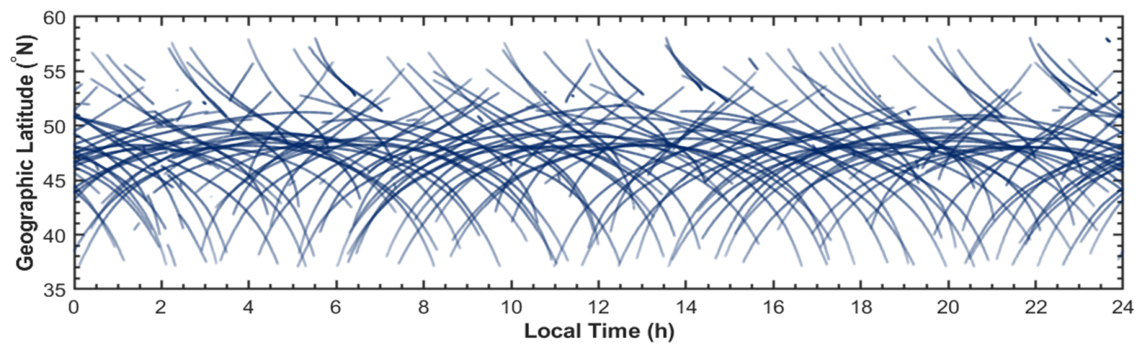
To examine this feature, 24 h of continuous IPP data from the OBE4 station (48.085° N, 11.278° E) on 1 July 2021, were used. The sampling interval was 30 s, yielding 2880 epochs. The dataset includes joint observations from GPS, BDS, Galileo, and GLONASS, with approximately 25 visible satellites per epoch on average. After low-elevation observations were excluded and data quality control was applied, approximately 72,000 valid IPPs were retained. Figure 1 shows their distribution in the Sun-fixed coordinate system.

Figure 1 shows that the IPPs are mainly concentrated within a limited latitudinal band near the station. Although Earth’s rotation allows single-station observations to cover a complete local-time cycle, the fixed geographic position of the receiver restricts IPP spatial sampling. In polynomial-based VTEC models, this localized distribution increases the correlation among the constant term, the latitudinal term, and the higher-order components in the design matrix. Taking the AQ model as an example, the constant column represents the background term, whereas the latitudinal column represents the first-order latitudinal gradient. When IPP latitude varies only within a narrow range, the linear correlation between these columns increases, causing the normal-equation matrix to become ill-conditioned. The normal-equation matrix is expressed as follows:

$$N=A^{\mathrm{T}}A$$

(16)

where ${\rm N}$ denotes the normal-equation matrix; and $A$ denotes the design matrix of the ionospheric VTEC inversion observation equations.

When the normal-equation matrix is inverted, a large condition number amplifies the effect of observation noise on parameter estimation and leads to numerical instability in conventional least-squares (LS) solutions. This is a key numerical challenge in single-station, single-epoch VTEC inversion. The LS coefficient solution is given by:

$$X={\left(A^{\mathrm{T}}A\right)}^{-1}{A}^{\mathrm{T}}L$$

(17)

where $X$ denotes the vector of coefficients to be estimated; and e denotes the known observation vector of the slant ionospheric delay.

A large condition number indicates that small perturbations in the observations may be amplified during parameter estimation. This problem becomes more severe when the model contains more spatial-gradient parameters or when the epoch interval is short. Although high-rate sampling improves temporal resolution, adjacent epochs usually have very similar satellite geometries and therefore do not necessarily provide independent geometric information. This trade-off motivates the use of a regularization strategy for robust single-epoch VTEC inversion.

2.4. Virtual-Observation-Based Tikhonov Regularization

Using the matrix observation model in Equations (14)–(16), the conventional LS estimation obtains the unknown parameter vector by minimizing the residual between the model prediction and the observation vector:

$${\min }_{\mathrm{X}}{‖AX-L‖}_2^2$$

(18)

For maritime single-station single-epoch VTEC inversion, the IPPs are usually distributed within a limited local region around the receiver. This localized spatial sampling increases the correlation among the columns of the design matrix, especially for VTEC models containing higher-order spatial-gradient parameters. As a result, the normal-equation matrix may become ill-conditioned, and small observation errors may be amplified during parameter estimation. This amplification leads to unstable VTEC model coefficients and discontinuous VTEC time series in conventional LS inversion.

To improve the numerical stability of the inversion, a Tikhonov regularization term is introduced into the LS objective function, as shown in:

$${\min }_X\left\{{‖AX-L‖}_2^2+\mathrm{\alpha }{‖\Omega X‖}_2^2\right\}$$

(19)

where $\mathrm{\alpha }$ is the regularization factor, and $\Omega$ is the selective structural matrix. The first term represents the fitting residual of the GNSS-derived ionospheric observation equations, whereas the second term imposes additional structural constraints on selected components of the unknown vector.

The Tikhonov-regularized objective function can be equivalently written as an augmented least-squares system, as shown in:

$$\left[\begin{array}{c}A\\ \sqrt{\mathrm{\alpha }}\Omega \end{array}\right]X=\left[\begin{array}{c}L\\ 0\end{array}\right]$$

(20)

This augmented system can also be written as two groups of equations, as shown in:

$$\left\{\begin{array}{l}AX=L\hfill \\ \sqrt{\mathrm{\alpha }}\Omega X=0\hfill \end{array}\right.$$

(21)

The first group of equations corresponds to the real GNSS-derived ionospheric observation equations. The second group does not come from physical GNSS measurements. Instead, it is an artificial constraint equation introduced by the Tikhonov regularization term. Therefore, the second group can be interpreted as a set of virtual observations. In this study, virtual observations refer to the equivalent observation-equation form of the Tikhonov regularization constraint. They are not additional GNSS measurements, but prior structural constraints imposed on selected model parameters to suppress unstable variations caused by weak single-station observation geometry.

In the proposed TVO method, the virtual observations are not imposed on all unknown parameters uniformly. The background VTEC coefficient, spatial-gradient coefficients, and receiver DCB parameters have different physical meanings and different sensitivities to observation geometry. The background VTEC coefficient represents the main VTEC level around the station, and the receiver DCB parameters represent instrumental biases. Directly penalizing these terms may introduce unnecessary bias into the estimated VTEC and receiver-bias parameters. In contrast, higher-order spatial-gradient coefficients are more sensitive to localized IPP distributions and strong column correlation in the design matrix. Therefore, TVO selectively imposes virtual-observation constraints on vulnerable spatial-gradient parameters while leaving the background VTEC coefficient and receiver DCB parameters unpenalized.

The regularization strength is determined according to the degree of ill-conditioning of the normal-equation matrix. In ill-conditioned LS inversion, small positive eigenvalues of the normal-equation matrix correspond to weakly constrained parameter directions. Observation noise can be amplified along these directions, leading to unstable VTEC model coefficients and discontinuous time series. Therefore, the condition number and eigenvalue distribution of the normal-equation matrix provide indicators of the instability level of the inversion system. A larger condition number indicates that the LS solution is more sensitive to observation noise and therefore requires stronger regularization to suppress unstable parameter variations. When the condition number is small, the regularization strength is reduced to avoid over-constraining otherwise stable models.

Regularization factors are determined for the four VTEC models, namely LP, SH, AQ, and FQ, by establishing a monotonic relationship between the regularization factor and the condition number of the normal-equation matrix. Since the four models have different numbers of unknown parameters and different spatial-basis structures, their eigenvalue distributions and sensitivities to weak observation geometry are also different. The LP model contains fewer spatial-gradient parameters and is less prone to over-parameterization, whereas the SH, AQ, and FQ models contain more flexible spatial terms and are more sensitive to localized IPP distributions and column correlation in the design matrix. Therefore, a single uniform expression for the regularization factor may not properly reflect the different ill-conditioning characteristics of these models.

For this reason, model-dependent expressions are adopted for the regularization factor. These expressions are not intended to serve as universal optimal parameter-selection rules. Instead, they provide a deterministic condition-number-aware scaling strategy for stabilizing single-station single-epoch VTEC inversion under weak observation geometry. The regularization factors are defined as follows:

$$\mathrm{\alpha }=\left\{\begin{array}{ll}\mathrm{median}(\mathrm{\lambda }(N))\cdot \sqrt{2\ln (\mathrm{p})}\hfill & (\mathrm{SH} \mathrm{model})\hfill \\ {\displaystyle \frac{{\mathrm{\lambda }}_{\max }(N)-{\mathrm{\lambda }}_2(N)}{{\mathrm{\lambda }}_{\max }(N)}}\hfill & (\mathrm{LP} \mathrm{model})\hfill \\ {\mathrm{\lambda }}_{\max }(N)\cdot \sqrt{{\displaystyle \frac{{\mathrm{\lambda }}_{\max }(N)}{{\mathrm{\lambda }}_{\min }(N)}}}\hfill & (\mathrm{AQ}/\mathrm{FQ} \mathrm{model})\hfill \end{array}\right.$$

(22)

where $\mathrm{\lambda }\left({\rm N}\right)$ represents the set of eigenvalues of the normal-equation matrix $N$; $\mathrm{p}$ is the total number of unknown parameters to be estimated in the observation equations; ${\mathrm{\lambda }}_{\max }\left({\rm N}\right)$, ${\mathrm{\lambda }}_2\left({\rm N}\right)$, and ${\mathrm{\lambda }}_{\min }\left({\rm N}\right)$ denote the largest eigenvalue, the second-largest eigenvalue, and the smallest positive eigenvalue of $N$, respectively.

The selective structural matrix $\Omega$ imposes constraints on higher-order spatial gradient parameters while leaving the background VTEC coefficient and receiver DCB parameters unpenalized. It is formulated as follows:

$$\Omega =\mathrm{d}\mathrm{i}\mathrm{a}\mathrm{g}\left({\mathrm{w}}_1,{\mathrm{w}}_2,\dots ,{\mathrm{w}}_{\mathrm{p}}\right)$$

(23)

where $\Omega$ denotes a $\mathrm{p}\times \mathrm{p}$ diagonal matrix; $\mathrm{d}\mathrm{i}\mathrm{a}\mathrm{g}$ denotes the diagonalization operator that maps the input vector ${\mathrm{w}}_1,{\mathrm{w}}_2,\dots {\mathrm{w}}_{\mathrm{p}}$ into a diagonal matrix, with its diagonal elements corresponding to the components of the input vector and its off-diagonal elements being zero; $\mathrm{p}$ is the total number of unknown parameters to be estimated in the observation equations; ${\mathrm{w}}_{\mathrm{i}}$ denotes the structural weight assigned to the $\mathrm{i}$-th parameter, ${\mathrm{w}}_{\mathrm{i}}=\left\{\begin{array}{ll}0,\hfill & {\mathrm{x}}_{\mathrm{i}}\in {\mathrm{S}}_0\hfill \\ 1,\hfill & {\mathrm{x}}_{\mathrm{i}}\in {\mathrm{S}}_{\mathrm{r}}\hfill \end{array}\right.$, ${\mathrm{S}}_0$ denotes the set of unpenalized parameters, including the background VTEC coefficient and receiver DCB parameters, rdenotes the set of regularized spatial-gradient parameters that are more sensitive to weak observation geometry and $\mathrm{i}$ denotes the index of the parameters to be estimated.

In complex maritime environments, the number of visible satellites per epoch may decrease, and the number of valid observations can be further reduced after low-elevation data are excluded. Under these conditions, the normal-equation matrix may approach rank deficiency. To improve numerical stability, a small stabilization term is introduced into the regularized normal equations. This term is used only to prevent matrix singularity and does not alter the condition-number-driven adaptive weighting among models. It is defined as follows:

$$\mathrm{\mu }=\mathrm{\epsilon }\cdot {\displaystyle \frac{\mathrm{t}\mathrm{r}\left(N\right)}{\mathrm{p}}}$$

(24)

where $\mathrm{\mu }$ denotes the numerical stabilization term; $\mathrm{p}$ represents the total number of unknown parameters to be estimated in the observation equations; and $\mathrm{t}\mathrm{r}$ denotes the trace operator; $\mathrm{\epsilon }$ is a small positive numerical stabilization constant. The parameter $\mathrm{\epsilon }$ is not introduced as an infinitesimal quantity or as a limiting process with $\mathrm{\epsilon }$ to 0. Instead, it is used as a small positive constant to prevent numerical singularity when the normal-equation matrix becomes nearly rank deficient. Its value is chosen sufficiently small so that it improves numerical invertibility without changing the dominant condition-number-aware regularization effect.

By adding the selective Tikhonov regularization term and the numerical stabilization term to the original LS normal equations, the final solution is obtained as follows:

$${\rm X}={\left(A^{\mathrm{T}}A+{\mathrm{\alpha }}^2{\Omega }^{\mathrm{T}}\Omega +\mathrm{\mu }{I}_{\mathrm{p}}\right)}^{-1}{A}^{\mathrm{T}}L$$

(25)

where $I_{\mathrm{p}}$ denotes the identity matrix of order $\mathrm{p}$. In this formulation, the real observation equations provide the data-fitting constraint, the virtual observations provide selective structural constraints, and the stabilization term prevents numerical singularity under extremely weak observation geometry.

For the AQ model in Equation (8), the coefficient ${\mathrm{a}}_0$ represents the background VTEC term, while ${\mathrm{a}}_1$, ${\mathrm{a}}_2$, and ${\mathrm{a}}_3$ represent spatial-gradient terms. In the TVO framework, ${\mathrm{a}}_0$ and the receiver DCB parameters are kept unpenalized, whereas the spatial-gradient coefficients are selectively constrained through the virtual-observation term. By preserving the physical meaning of the background VTEC coefficient and receiver DCB parameters while constraining vulnerable spatial-gradient parameters, TVO reduces the influence of local geometric degradation on higher-order model coefficients and improves the numerical stability of single-station single-epoch VTEC inversion.

3. Experimental Analysis and Results

3.1. European Terrestrial GNSS Stations

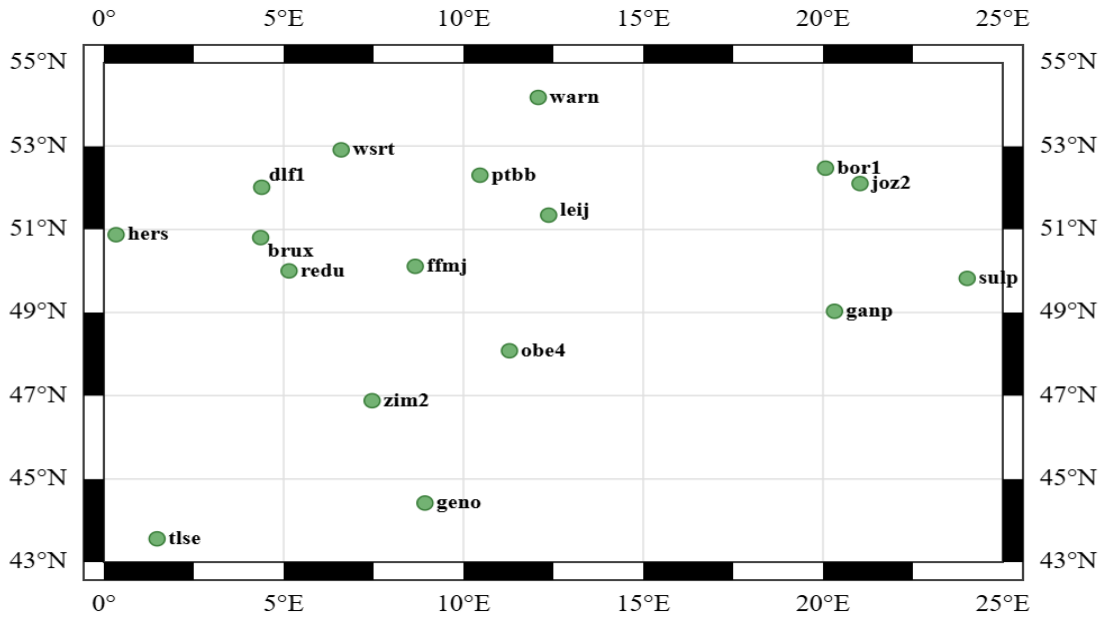
After formulating the model, this study evaluates the ability of TVO to mitigate ill-conditioning through a series of experiments. First, this study analyzed the condition numbers of the normal-equation matrices under different VTEC models and epoch intervals using data from 17 European GNSS stations. Figure 2 illustrates the geographic distribution of these stations, providing spatial context for the subsequent experiments. Then, the TVO was compared with the conventional LS approach using VTEC values interpolated from IGS GIM as an external reference to evaluate its capability in mitigating ill-conditioning. Finally, data from buoy platforms in the South China Sea were employed to assess the applicability of the proposed method under dynamic marine observation conditions.

The geomagnetic background of the experimental periods was also checked before evaluating the VTEC inversion results. This check was performed to distinguish the numerical stability of the inversion method from possible ionospheric variations caused by geomagnetic disturbances. Kp and Ap were obtained from GFZ, and Dst was obtained from WDC Kyoto. The geomagnetic conditions during the terrestrial and maritime experiments are summarized in

Table 1. Geomagnetic activity during the experimental periods. Kp and Ap are from GFZ, and Dst is from WDC Kyoto. Dstmin is given in nT.

Period	Data	Kp	Ap	Dst min	State
7 January 2021	17 Eu stations	0.33–3.00	5	−15	Quiet–unsettled
19–25 May 2025	SCS buoy	0.67–4.00	4–12	−23	Quiet–mildly active

.

As shown in Table 1, no strong geomagnetic storm occurred during either experimental period. Therefore, the comparison between LS and TVO mainly reflects the influence of observation geometry and numerical stability rather than severe geomagnetic-storm-driven ionospheric disturbances.

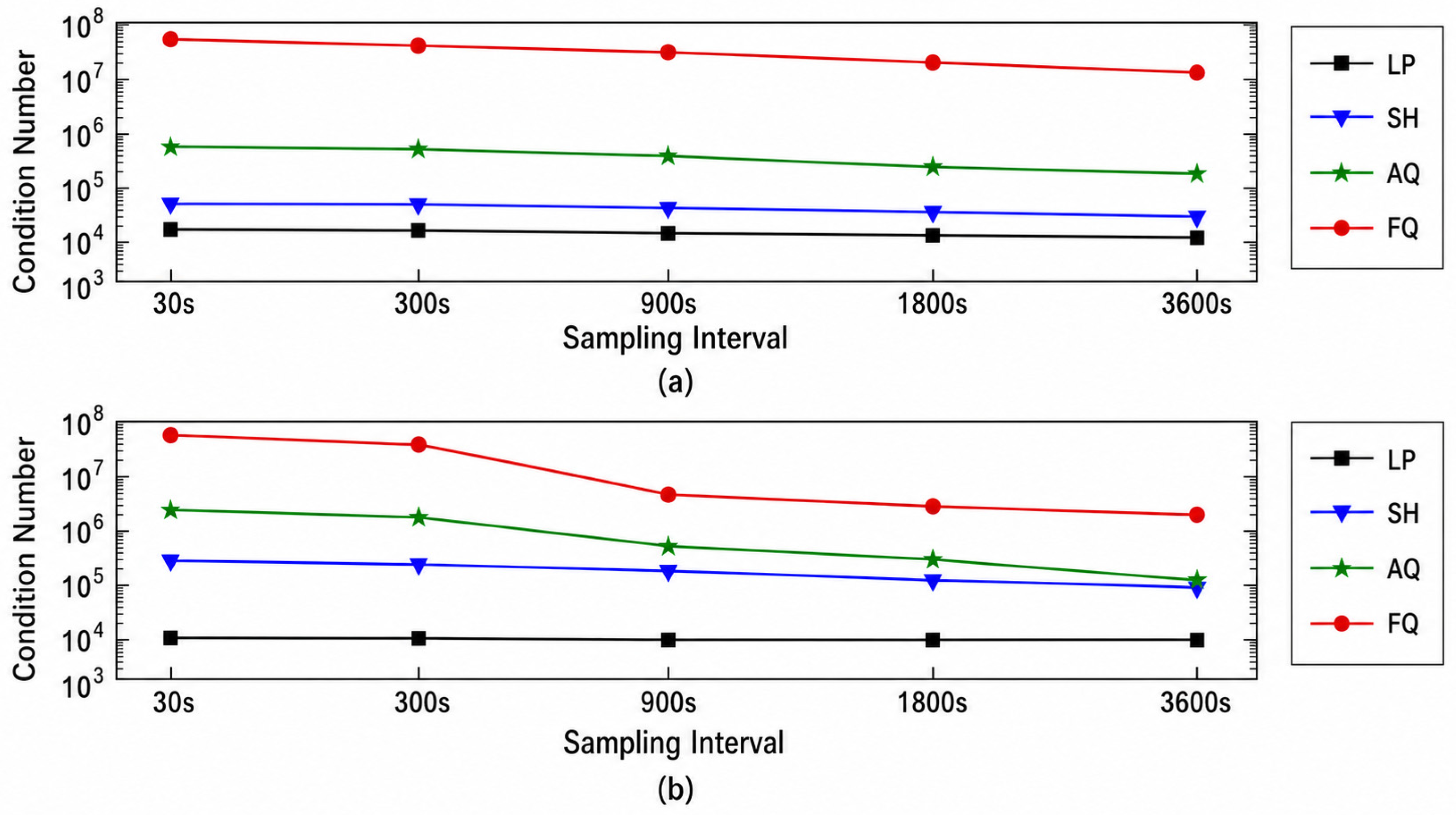
A larger condition number indicates that observation noise is more likely to be amplified during parameter estimation. In this study, the condition number of the normal-equation matrix is used to quantify model ill-conditioning. Because the condition number of the normal-equation matrix is generally larger than that of the original design matrix, it more directly reflects the instability risk of the LS solution. When the condition number becomes large, conventional LS may fail to provide a stable solution, which motivates the introduction of TVO. Figure 3 shows the condition numbers of the LS normal-equation matrices for the four VTEC models at different epoch intervals.

The corresponding condition numbers are listed in

Table 2. Condition numbers for the OBE4 station.

Model/Epoch	30 s	300 s	900 s	1800 s	3600 s
LP	5.2774 × 103	5.0585 × 103	4.6163 × 103	4.2207 × 103	3.8184 × 103
SH	1.4136 × 104	1.3281 × 104	1.1778 × 104	1.0195 × 104	8.3547 × 103
AQ	1.9364 × 105	1.7448 × 105	1.3964 × 105	8.2262 × 104	6.1953 × 104
FQ	3.7434 × 107	3.0609 × 107	2.0583 × 107	1.2080 × 107	7.5834 × 106

and

Table 3. Average condition numbers across the 17 stations.

Model/Epoch	30 s	300 s	900 s	1800 s	3600 s
LP	4.9898 × 103	4.6078 × 103	4.0865 × 103	3.7203 × 103	3.3273 × 103
SH	5.2925 × 105	4.3845 × 105	3.0488 × 105	1.9520 × 105	1.3290 × 105
AQ	7.4257 × 106	4.5906 × 106	1.0542 × 106	5.6841 × 105	1.8195 × 105
FQ	3.4265 × 108	1.9478 × 108	1.4259 × 107	8.4008 × 106	5.4754 × 106

. Because of their large magnitudes, all values are reported in scientific notation.

The OBE4 result and the average over the 17 independent single-station cases both show that matrix ill-conditioning varies substantially across VTEC models and epoch intervals. Overall, the LP model has the lowest condition number and therefore the weakest ill-conditioning. The SH and AQ models have larger condition numbers because they introduce additional spatial basis functions. The FQ model, which contains the largest number of parameters, is the most susceptible to ill-conditioning in the normal-equation matrix. As the epoch interval increases, the condition number for a given model generally decreases, indicating that satellite-geometry variation over longer time spans helps reduce column correlation. Conversely, although 30 s high-rate sampling provides higher temporal resolution, adjacent epochs have highly similar observation geometries. This similarity strengthens the correlation among parameter columns in the design matrix and reduces the stability of the LS solution.

It should also be noted that the dependence of the condition number on the epoch interval is not exactly the same between the OBE4 result and the 17-station averaged result. This difference is mainly caused by station-dependent observation geometry. For a single station, the condition number is controlled by the local IPP distribution, visible-satellite geometry, constellation combination, and data-quality screening at that station. Therefore, the OBE4 result reflects the specific geometric characteristics of one station. In contrast, the 17-station averaged result combines stations with different IPP distributions and different degrees of geometric constraint. Some stations may have more clustered IPPs or stronger column correlation in the design matrix, especially for SH, AQ, and FQ models with more spatial-gradient parameters. As a result, the averaged condition numbers can be larger and may decrease more sharply as the epoch interval increases. This difference does not contradict the main conclusion; rather, it indicates that the sensitivity of the condition number to the epoch interval is station dependent and becomes more pronounced for high-order VTEC models.

The 30 s high-rate epoch interval therefore involves a clear trade-off: it helps preserve rapid ionospheric variations but also exacerbates ill-conditioning in single-station VTEC inversion. Considering the demand for high temporal resolution in real-time maritime monitoring, the subsequent experiments use 30 s empirical data and focus on comparing the time-series stability and RMS differences in TVO and LS under ill-conditioned observation conditions.

To evaluate the effectiveness and robustness of TVO in single-station VTEC inversion, experiments were conducted using data from the representative European mid-latitude station OBE4 and 17 surrounding stations on 1 July 2021. The LS method and TVO were used to estimate VTEC model parameters and derive the corresponding VTEC time series. VTEC values interpolated from IGS GIM products were used as an external reference, and RMS differences between the inverted VTEC series and the GIM reference values were adopted as the main evaluation metric. It should be emphasized that GIM products are not treated as an absolute accuracy benchmark; rather, they provide an independent external reference for comparing the relative stability and consistency of different estimation methods within the same framework.

To assess the improvement of TVO over LS in terrestrial station scenarios, VTEC inversion results from different models at OBE4 were examined using a 30 s sampling interval. The results are shown in Figure 4. The solid black line represents the GIM-interpolated VTEC reference, the dashed blue line denotes the VTEC series obtained by LS, and the solid red curve represents the VTEC series derived using TVO.

Figure 4 shows that, as the number of model parameters increases, local fluctuations in the LS series become more pronounced and deviate from the GIM reference during some periods. After TVO is introduced, the VTEC series from different models show better overall continuity and trends that are more consistent with the GIM reference, while the main diurnal variation remains preserved. Because GIM products are temporally and spatially smoothed, VTEC series obtained from 30 s high-rate sampling may contain both real small- to medium-scale perturbations and observation noise. Therefore, TVO is evaluated mainly in terms of RMS differences and time-series stability. For quantitative comparison, the RMS difference between the estimated VTEC and the GIM-interpolated VTEC reference was calculated as

$$\mathrm{RMS}=\sqrt{{\displaystyle \frac{1}{\mathrm{n}}}{\displaystyle \sum _{\mathrm{i}=1}^{\mathrm{n}}{\left({\mathrm{VTEC}}_{\mathrm{est},\mathrm{i}}-{\mathrm{VTEC}}_{\mathrm{GIM},\mathrm{i}}\right)}^2}}$$

(26)

where $\mathrm{V}\mathrm{T}\mathrm{E}{\mathrm{C}}_{\mathrm{e}\mathrm{s}\mathrm{t},\mathrm{i}}$ denotes the VTEC estimated by LS or TVO at epoch $\mathrm{i}$, $\mathrm{V}\mathrm{T}\mathrm{E}{\mathrm{C}}_{\mathrm{G}\mathrm{I}\mathrm{M},\mathrm{i}}$ denotes the GIM-interpolated VTEC reference at the same epoch and location, and $\mathrm{n}$ is the number of valid epochs. In this study, the GIM-interpolated VTEC is used as an external reference for relative comparison rather than as an absolute true VTEC value.

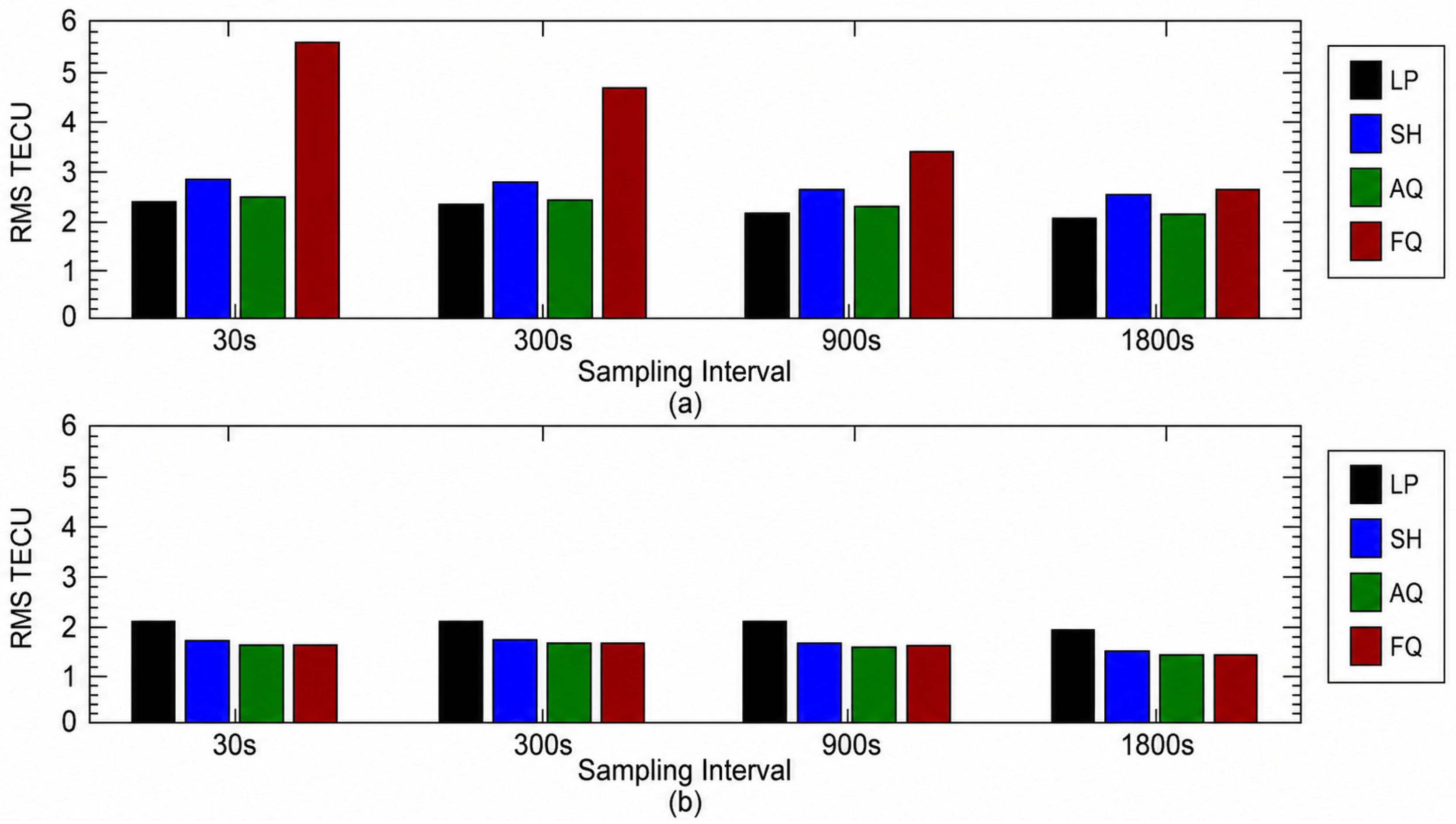
The comparison in Figure 5 includes the four models (LP, SH, AQ, and FQ) at epoch intervals from 30 s to 1800 s.

The corresponding values are listed in

Table 4. RMS differences relative to the GIM-interpolated VTEC reference from the LS method at OBE4. Unit: TECU.

Model/Epoch	30 s	300 s	900 s	1800 s
LP	2.317	2.258	2.146	1.987
SH	2.813	2.754	2.624	2.520
AQ	2.479	2.410	2.280	2.095
FQ	6.095	4.864	3.419	2.757

and

Table 5. RMS differences relative to the GIM-interpolated VTEC reference from the TVO method at OBE4. Unit: TECU.

Model/Epoch	30 s	300 s	900 s	1800 s
LP	2.167	2.142	2.124	1.978
SH	1.759	1.708	1.631	1.532
AQ	1.702	1.657	1.575	1.481
FQ	1.701	1.648	1.574	1.480

.

The statistics show that, at OBE4, the average RMS values of the LP, SH, AQ, and FQ models obtained with TVO are all lower than the corresponding LS results. The RMS reductions are approximately 3.41% for LP, 30.75% for AQ, 38.10% for SH, and 62.63% for FQ, yielding an overall average reduction of 39.20% across the four models. These results indicate that the stabilizing effect of TVO becomes more pronounced as model complexity increases.

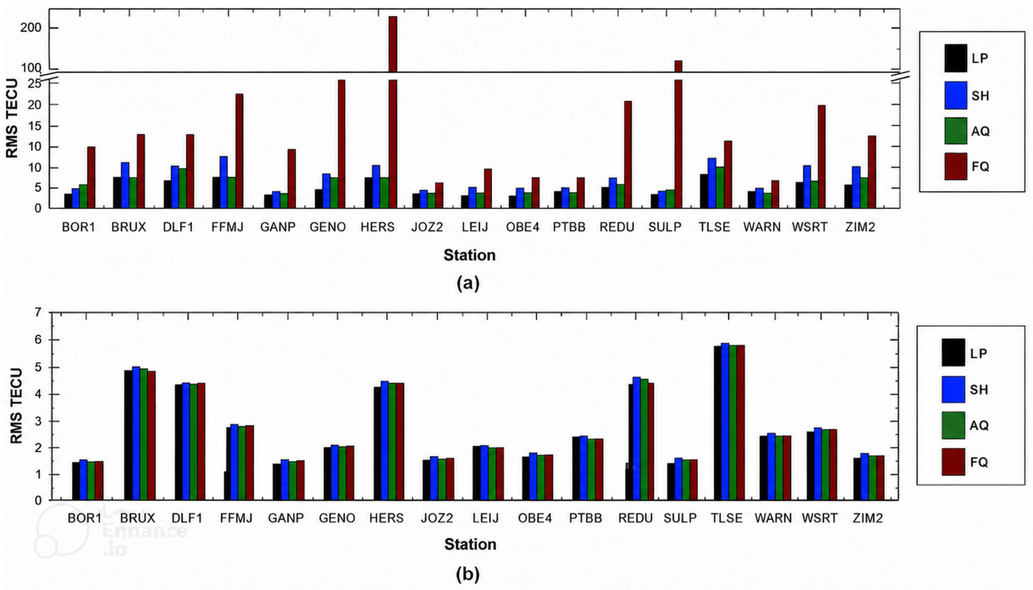
To reduce the influence of local observation conditions and further assess TVO in terrestrial single-station scenarios, the experiment was extended to 17 stations in the European mid-latitude region during the same period. Figure 6a,b present the RMS statistics for LS and TVO, respectively, for the four VTEC models at a 30 s sampling interval.

Figure 6 shows that LS generally yields larger RMS values for models with more parameters, indicating that model ill-conditioning adversely affects parameter-estimation stability. The corresponding LS RMS results are listed in

Table 6. Mean RMS differences relative to the GIM-interpolated VTEC reference from the LS method across 17 stations. Unit: TECU.

Model/Epoch	30 s	300 s	900 s	1800 s
LP	2.952	2.896	2.813	2.728
SH	4.712	4.587	4.359	4.106
AQ	3.198	3.099	2.958	2.841
FQ	30.218	19.894	6.519	5.126

. In contrast, TVO maintains more stable RMS levels across the 17 stations and four models, with no obvious error amplification as model complexity increases. For the 17-station results, LS produces higher RMS values for the FQ model, and some stations also show relatively large deviations for the SH model. After TVO is applied, the RMS values of the AQ, SH, and FQ models improve noticeably, with most terrestrial-station results stabilizing within 2–3 TECU. These results demonstrate that TVO effectively mitigates error amplification caused by matrix ill-conditioning and is particularly suitable for VTEC models with more parameters and stronger column correlation.

3.2. Sensitivity Analysis of the Regularization Factor

To further evaluate the robustness of the proposed condition-number-aware regularization factor, a sensitivity analysis was conducted using the terrestrial experiment dataset. The test was performed using the 17 European mid-latitude stations on 1 July 2021 at a 30 s sampling interval. The GIM-interpolated VTEC was used as the external reference, and the RMS difference between the estimated VTEC and the GIM-interpolated VTEC was used as the evaluation metric.

For each VTEC model, the adaptive regularization factor obtained from the model-dependent mapping strategy was multiplied by a scale coefficient. The tested scale coefficients were 0.5, 0.8, 1.0, 1.2, and 1.5. The scaled regularization factor is expressed as

$${\mathrm{\alpha }}_{\mathrm{s}}=\mathrm{s}{\mathrm{\alpha }}_{\mathrm{s}}$$

(27)

where $\mathrm{s}$ denotes the scale coefficient. During the sensitivity analysis, the observation data, VTEC model structure, selective structural matrix, numerical stabilization term, and GIM reference were kept unchanged. Therefore, the comparison only reflects the influence of the regularization-factor magnitude.

Table 7. Mean RMS differences relative to the GIM-interpolated VTEC reference from the TVO method across 17 stations. Unit: TECU.

Model/Epoch	30 s	300 s	900 s	1800 s
LP	2.866	2.857	2.799	2.722
SH	2.904	2.867	2.798	2.720
AQ	2.890	2.853	2.784	2.707
FQ	2.889	2.854	2.786	2.709

summarizes the mean RMS values of the LP, SH, AQ, and FQ models under different scale coefficients.

Table 8. Sensitivity analysis of the regularization factor. The RMS values are averaged over the 17 European mid-latitude stations on 1 July 2021 at a 30 s sampling interval. The GIM-interpolated VTEC is used as the external reference. Unit: TECU.

Scale Coefficient	LP RMS/	SH RMS	AQ RMS	FQ RMS	Mean RMS
0.5 $\mathrm{\alpha }$	3.018	3.071	3.026	3.044	3.040
0.8 $\mathrm{\alpha }$	2.884	2.889	2.874	2.883	2.883
1.0 $\mathrm{\alpha }$	2.866	2.904	2.890	2.889	2.887
1.2 $\mathrm{\alpha }$	2.875	2.896	2.881	2.876	2.882
1.5 $\mathrm{\alpha }$	2.942	2.978	2.946	2.936	2.951

presents the sensitivity analysis of the regularization factor. The mean RMS values of the LP, SH, AQ, and FQ models obtained with TVO are consistently lower than those obtained with conventional LS. Specifically, RMS decreases by 81.80% for FQ, 36.45% for SH, and 7.13% for AQ. Because the LS result for the LP model is already relatively stable, its reduction is modest, at 1.27%. Overall, the average RMS reduction across the four models and 17 terrestrial stations reaches 56.30%. These results show that TVO can adaptively adjust the regularization strength according to the condition number of the normal-equation matrix, thereby improving the numerical stability of single-station VTEC inversion in terrestrial scenarios.

The results show that the RMS values remain relatively stable when the scale coefficient varies from 0.8 $\mathrm{\alpha }$ to 1.2 $\mathrm{\alpha }$. Although the minimum RMS is not always obtained at 1.0 $\mathrm{\alpha }$ for every individual model, the differences among 0.8 $\mathrm{\alpha }$, 1.0 $\mathrm{\alpha }$, and 1.2 e are small. This indicates that the proposed condition-number-aware regularization factor is not highly sensitive to moderate scaling perturbations. The larger RMS values obtained with 0.5 $\mathrm{\alpha }$ indicate that insufficient regularization may fail to suppress unstable components associated with weak observation geometry. In contrast, the increase in RMS observed with 1.5 $\mathrm{\alpha }$ suggests that excessive regularization may over-constrain the spatial-gradient parameters and reduce the flexibility of the VTEC model. The default 1.0 $\mathrm{\alpha }$ does not necessarily produce the absolute minimum RMS for every individual model, but it remains within the stable range and provides a balanced solution between noise suppression and model flexibility. Therefore, the proposed adaptive regularization factor can be regarded as a robust deterministic choice.

3.3. Maritime Buoy Experimen

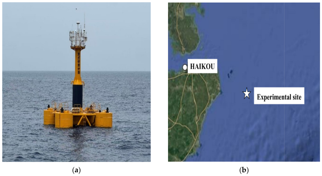
Building on the terrestrial experiments, this study further evaluates TVO in challenging maritime environments. Marine buoy platforms are affected by platform motion, sea-surface multipaths, and time-varying observation noise; therefore, their data quality and observation geometry are generally less favorable than those of fixed terrestrial stations. Such data provide a suitable test case for assessing method robustness under more challenging conditions. The experimental system, including a GNSS antenna, meteorological sensors, a GNSS receiver, and an industrial computer, was deployed on a buoy platform in the South China Sea (19.64° N, 111.61° E). Dual-frequency pseudorange and carrier-phase observations collected over seven consecutive days from 19 to 25 May 2025, were used as the raw data. The buoy deployment and experimental site are shown in Figure 7.

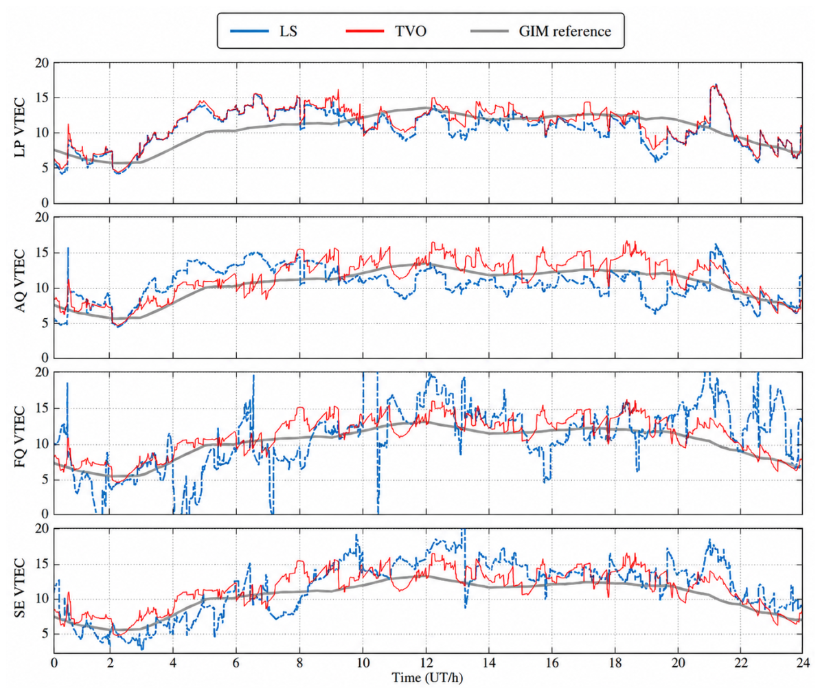
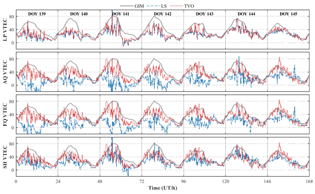
VTEC inversion tests were conducted using measured buoy data at 30 s intervals. Figure 8 shows the VTEC series obtained from different models under LS and TVO. The solid black line represents the GIM-interpolated VTEC reference, the dashed blue line denotes the LS-derived VTEC series, and the solid red curve represents the TVO-derived VTEC series.

Figure 8 shows that the VTEC series derived with TVO has better temporal continuity than the LS series, and its variation trend is more consistent with the external reference. The negative VTEC values appearing in some LS-derived maritime time series are non-physical estimates caused by the instability of the unconstrained LS solution under weak observation geometry. They should not be interpreted as physically meaningful ionospheric states. Instead, these values indicate abnormal local oscillations caused by parameter coupling and noise amplification in the LS inversion. They are retained in Figure 8 to illustrate the instability of LS under maritime single-station conditions. After applying TVO, the selective regularization constraints suppress these unstable components, resulting in a more physically reasonable and temporally continuous VTEC series.

It can also be observed from Figure 8 that the LS and TVO results are relatively similar for the LP model, whereas larger differences appear for the SH, AQ, and FQ models. This phenomenon is mainly related to model complexity. The LP model contains fewer spatial-gradient parameters and has a lower risk of over-parameterization under sparse maritime IPP distributions. Therefore, its normal-equation matrix is less severely ill-conditioned, and the stabilizing effect of TVO is less pronounced. In contrast, the SH, AQ, and FQ models contain more flexible spatial terms and are more sensitive to weak observation geometry, localized IPP distributions, and column correlation in the design matrix. Under these conditions, the unconstrained LS solution is more likely to produce local oscillations or abnormal amplitude variations, while TVO suppresses unstable spatial-gradient components through selective virtual-observation constraints. As a result, the improvement brought by TVO becomes more evident for models with more spatial parameters.

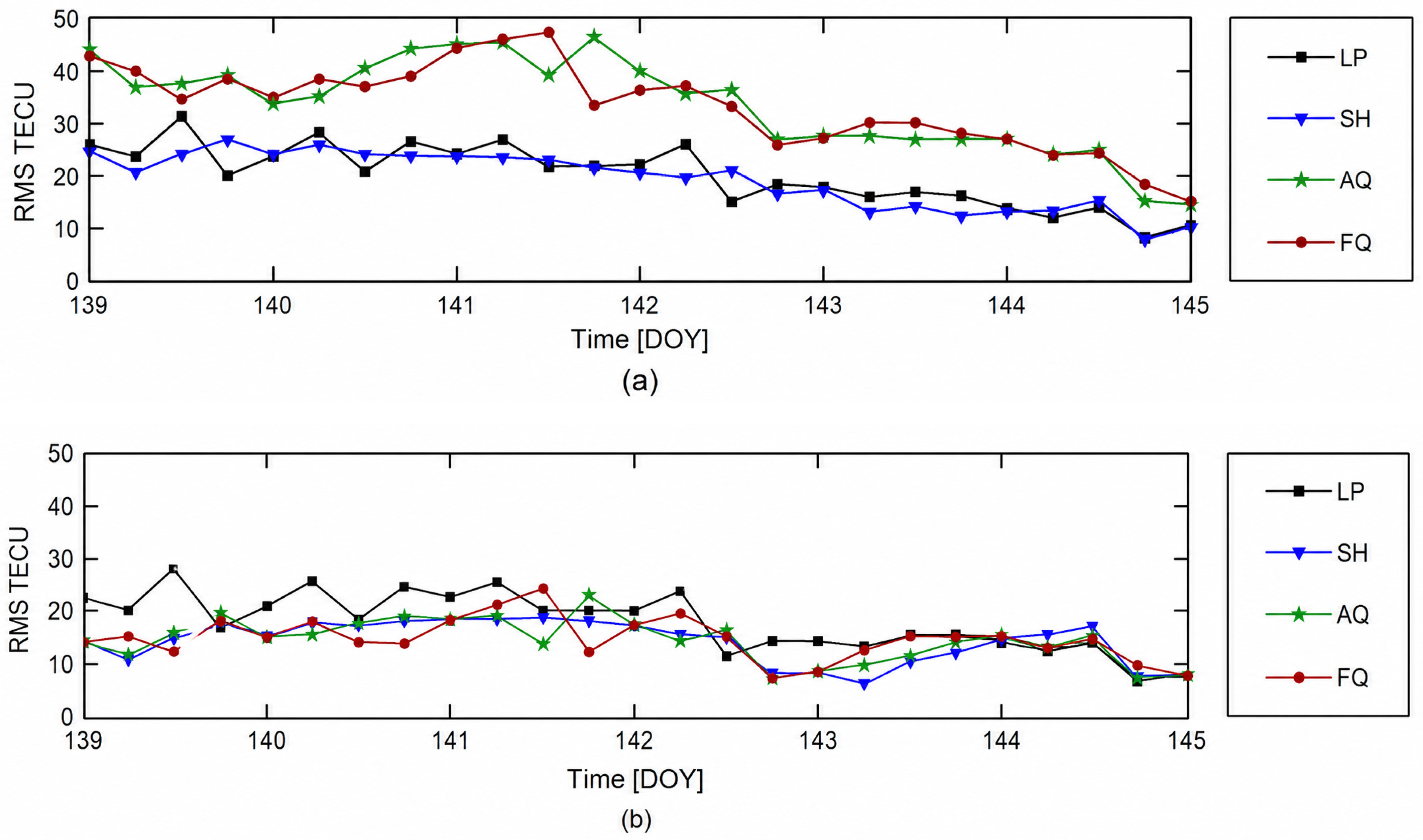
It should be noted that GIM reference values in maritime regions are themselves affected by product resolution and sparse terrestrial-station coverage. Therefore, this study emphasizes the stability improvement of TVO relative to LS rather than treating GIM as an absolute accuracy benchmark. To further verify TVO in maritime single-station scenarios, Figure 9 presents the daily RMS variations and the corresponding mean RMS values for each model under LS and TVO at a 30 s interval over the seven-day period.

Table 9. Daily RMS differences relative to the GIM-interpolated VTEC reference from the LS method for the buoy platform over the seven-day period. Unit: TECU.

Model\DOY	139	140	141	142	143	144	145
LP	25.686	23.744	24.082	22.076	17.687	13.614	10.448
SH	24.543	23.942	23.739	20.531	17.131	13.032	10.075
AQ	44.132	33.753	45.348	40.008	27.472	26.778	14.496
FQ	42.670	34.947	44.714	36.315	27.029	26.881	15.087

and

Table 10. Daily RMS differences relative to the GIM-interpolated VTEC reference from the TVO method for the buoy platform over the seven-day period. Unit: TECU.

Model\DOY	139	140	141	142	143	144	145
LP	22.148	20.717	22.402	19.998	14.129	13.916	7.8791
SH	14.571	15.260	18.506	17.444	8.6599	15.023	7.6191
AQ	14.344	15.146	18.491	17.447	8.7776	15.375	7.9518
FQ	14.160	15.072	18.386	17.398	8.7166	15.243	7.9213

list the detailed daily RMS statistics for each model during this period.

The statistical results in Table 9 and Table 10 indicate that the overall RMS in the maritime experiment is higher than that in the terrestrial-station experiments, mainly because of buoy motion, sea-surface multipaths, hardware-environment effects, and challenging marine observation conditions. Under these complex conditions, TVO effectively reduces local amplitude anomalies and error amplification in LS solutions. The improvements are particularly pronounced for the AQ and FQ models: their seven-day average RMS values decrease from 33.141 TECU and 32.520 TECU to 13.933 TECU and 13.842 TECU, corresponding to reductions of approximately 58% and 57%, respectively. The average RMS values for the LP and SH models decrease from 19.620 TECU and 18.999 TECU to 17.313 TECU and 13.869 TECU, corresponding to reductions of approximately 12% and 27%, respectively. Overall, the average RMS difference relative to the GIM-interpolated VTEC reference across the four models decreases from 26.07 TECU to 14.74 TECU, corresponding to a reduction of approximately 43.46%. The similar RMS levels of the SH, AQ, and FQ models after TVO indicate that the proposed selective regularization suppresses unstable higher-order components and reduces the sensitivity of the inversion results to model over-parameterization under weak maritime observation geometry. These results demonstrate that TVO mitigates LS instability caused by ill-conditioned matrices and yields more stable VTEC inversion results in complex maritime environments.

4. Discussion

The results of this study confirm that maritime single-station VTEC inversion is strongly affected by limited observation geometry. Compared with global or regional ionospheric modeling, single-station observations provide fewer spatial constraints because the IPPs are usually concentrated within a limited region around the receiver. This restricted sampling increases the correlation among the columns of the design matrix and makes the normal-equation matrix ill-conditioned. The condition-number analysis shows that the ill-conditioning becomes more severe when the epoch interval is shortened or when the model complexity increases. In particular, the FQ model has the largest condition numbers because it contains more spatial-gradient parameters, making it more sensitive to observation noise under sparse or clustered IPP distributions. These results indicate that the main difficulty is not only the observation noise itself, but also the amplification of that noise through an ill-conditioned least-squares VTEC inversion system.

The proposed TVO method improves the stability of the inversion by introducing condition-number-aware Tikhonov regularization. Its main difference from conventional Tikhonov regularization lies in two aspects. First, the regularization factor is explicitly linked to the condition number of the normal-equation matrix, so that stronger regularization is applied when the LS system becomes more ill-conditioned, whereas weaker regularization is used when the matrix is relatively stable. Second, the structural matrix is designed to selectively penalize higher-order spatial-gradient parameters, while the background VTEC term and receiver DCB parameters are not directly penalized. This design suppresses unstable components caused by weak single-station geometry without strongly biasing the physically meaningful background term or the receiver instrumental bias. This problem-oriented design also differs from commonly used Tikhonov parameter-selection strategies. Classical approaches, such as the L-curve criterion, generalized cross-validation, and discrepancy-principle-based methods, are usually designed to balance data fitting and solution stability in general inverse problems. These methods are valuable for many offline inversion problems, but they may require repeated solutions under different regularization parameters, reliable noise-level information, or a relatively stable observation system. In contrast, the objective of the proposed TVO method is not to develop a universal optimal regularization-parameter selection rule, but to provide a practical stabilization strategy for single-station single-epoch VTEC inversion. Therefore, the regularization strength is linked directly to the condition number of the normal-equation matrix and combined with the model-aware structural matrix. This makes the method more suitable for high-temporal-resolution maritime applications, where the observation geometry may change rapidly and the inversion system may become ill-conditioned at individual epochs.

The terrestrial experiments demonstrate that TVO is effective for improving the numerical stability of single-station VTEC inversion. For the 17 European stations, the average RMS difference reduction relative to the GIM-interpolated VTEC reference across the four VTEC models reaches 56.30%, and most terrestrial-station RMS differences remain within 2–3 TECU. The improvement is especially evident for models with more parameters, such as FQ and SH, because these models are more vulnerable to ill-conditioning in conventional LS estimation. The maritime buoy experiment further shows that TVO can suppress local discontinuities and amplitude anomalies under more challenging marine observation conditions. The overall average RMS difference relative to the GIM-interpolated VTEC reference decreases from 26.07 TECU to 14.74 TECU, indicating improved temporal continuity and relative consistency.

It should be emphasized that the objective of this study is to evaluate whether TVO can stabilize an ill-conditioned least-squares VTEC inversion problem under constrained observation geometry. The GIM products are used as external references to compare the relative consistency and time-series stability of different inversion methods, rather than as absolute true VTEC values. This is particularly important in maritime regions, where GIM accuracy may be affected by sparse terrestrial-station coverage and limited spatial resolution. Therefore, the RMS-difference reduction reported in this study should be interpreted as an improvement in numerical stability and consistency with the GIM-interpolated external reference, not as a complete independent validation of absolute VTEC accuracy. Several limitations remain. First, the current experiments are based on selected European terrestrial stations and one South China Sea buoy observation period. Additional tests are needed under different latitudes, seasons, solar activity levels, and geomagnetic conditions. Second, although TVO reduces numerical artifacts caused by ill-conditioning, further validation is required to ensure that real ionospheric disturbances are preserved rather than over-smoothed. Third, the present validation mainly relies on GIM products as external references. Future work should incorporate more independent observations, such as radio occultation electron density profiles, ionosonde measurements, nearby buoy data, shipborne GNSS observations, and multi-source GIM products. These extensions would help further evaluate the applicability of TVO for real-time maritime ionospheric monitoring and GNSS delay correction.

5. Conclusions

This study investigated ill-conditioning in LS solutions for VTEC models caused by degraded GNSS observation geometry at maritime single stations. The analysis shows that concentrated IPP distributions around a single station increase design-matrix column correlation, causing the normal-equation matrix to become ill-conditioned and making both VTEC model parameters and inverted time series sensitive to observation noise. To address this issue, a TVO method was proposed that uses a condition-number-aware adaptive regularization strategy to reduce the sensitivity of LS solutions to ill-conditioned matrices.

Using data from the European mid-latitude station OBE4 and 17 surrounding stations, the condition numbers of the normal-equation matrices for the LP, SH, AQ, and FQ models were analyzed across different epoch intervals. The results show that increasing model complexity and shortening the epoch interval both exacerbate ill-conditioning, with the FQ model showing the most pronounced effect under 30 s high-rate sampling. Terrestrial experiments demonstrate that TVO improves the time-series stability of models with more parameters, with average RMS difference reductions relative to the GIM-interpolated VTEC reference of 39.20% at OBE4 and 56.30% across the 17 stations; most terrestrial RMS differences remain within 2–3 TECU. The sensitivity analysis further shows that the proposed regularization factor remains stable under moderate scaling perturbations, indicating that the deterministic parameter design is not highly sensitive to small changes in the regularization strength.

Maritime validation using South China Sea buoy data collected from 19 to 25 May 2025 further indicates that TVO reduces local anomalies in LS inversion series and improves consistency with the GIM-interpolated VTEC reference. The overall average RMS difference relative to the GIM-interpolated VTEC reference across the four models decreases from 26.07 TECU to 14.74 TECU, representing an approximately 43.46% reduction.

In summary, the proposed TVO method establishes a model-aware adaptive constraint mechanism based on the condition number of the normal-equation matrix. It alleviates ill-conditioning caused by insufficient observation geometry in single-station VTEC inversion and improves solution stability under complex maritime observation conditions. The main value of the method is its ability to stabilize high-temporal-resolution single-epoch inversion without relying on a dense reference-station network or long temporal smoothing windows. Because the IGS GIM products used as external references are still limited by spatial resolution and station distribution over maritime regions, future work should incorporate multi-source GIM products, radio occultation observations, nearby buoy data, and shipborne GNSS observations to enable more independent accuracy validation of maritime VTEC inversion results.

6. Patents

The method reported in this manuscript is related to a Chinese patent application entitled “A Model-Aware Regularization Method for Maritime Single-Station Single-Epoch VTEC Estimation”, Chinese Patent Application No. 202610492200.6, filed on 15 April 2026. The patent application is currently under examination.

References

Schaer, S. Mapping and Predicting the Earth’s Ionosphere Using the Global Positioning System; Institut für Geodäsie und Photogrammetrie, Eidg. Technische Hochschule Zürich: Zürich, Switzerland, 1999. [Google Scholar]
Yuan, Y.; Huo, X.; Zhang, B. Research progress of precise models and correction for GNSS ionospheric delay in China over recent years. Acta Geod. Et Cartogr. Sin.2017, 46, 1364–1378. [Google Scholar]
Yao, Y.; Gao, X. Research Progress and Prospect of Monitoring Ionosphere by GNSS Technique. Geomat. Inf. Sci. Wuhan Univ.2022, 47, 1728–1739. [Google Scholar] [CrossRef]
Li, W.; Li, Z.; Wang, N.; Liu, A.; Zhou, K.; Yuan, H.; Krankowski, A. A Satellite-Based Method for Modeling Ionospheric Slant TEC from GNSS Observations: Algorithm and Validation. GPS Solut.2021, 26, 14. [Google Scholar] [CrossRef]
Mannucci, A.J.; Wilson, B.D.; Yuan, D.N.; Ho, C.H.; Lindqwister, U.J.; Runge, T.F. A Global Mapping Technique for GPS-Derived Ionospheric Total Electron Content Measurements. Radio Sci.1998, 33, 565–582. [Google Scholar] [CrossRef]
Juan, J.M.; Hernandez-Pajares, M.; Sanz, J.; Ramos-Bosch, P.; Aragon-Angel, A.; Orus, R.; Ochieng, W.; Feng, S.; Jofre, M.; Coutinho, P.; et al. Enhanced Precise Point Positioning for GNSS Users. IEEE Trans. Geosci. Remote Sens.2012, 50, 4213–4222. [Google Scholar] [CrossRef]
Lanyi, G.E.; Roth, T. A Comparison of Mapped and Measured Total Ionospheric Electron Content Using Global Positioning System and Beacon Satellite Observations. Radio Sci.1988, 23, 483–492. [Google Scholar] [CrossRef]
Liu, T.; Zhang, B.; Yuan, Y.; Li, Z.; Wang, N. Multi-GNSS Triple-Frequency Differential Code Bias (DCB) Determination with Precise Point Positioning (PPP). J. Geod.2019, 93, 765–784. [Google Scholar] [CrossRef]
Ya’acob, N.; Abdullah, M.; Ismail, M. Determination of GPS Total Electron Content Using Single Layer Model (SLM) Ionospheric Mapping Function. Int. J. Comput. Sci. Netw. Secur.2008, 8, 154–160. [Google Scholar]
Zhang, B. Three Methods to Retrieve Slant Total Electron Content Measurements from Ground-Based GPS Receivers and Performance Assessment. Radio Sci.2016, 51, 972–988. [Google Scholar] [CrossRef]
Hernández-Pajares, M.; Juan, J.M.; Sanz, J.; Orus, R.; Garcia-Rigo, A.; Feltens, J.; Komjathy, A.; Schaer, S.C.; Krankowski, A. The IGS VTEC Maps: A Reliable Source of Ionospheric Information since 1998. J. Geod.2009, 83, 263–275. [Google Scholar] [CrossRef]
Yuan, Y.; Ou, J. Study on the New Methods of Correcting Ionospheric Delay and Ionospheric Model Using GPS Data. J. Univ. Chin. Acad. Sci.2002, 19, 209–214. [Google Scholar] [CrossRef]
Yuan, Y.; Ou, J. A Generalized Trigonometric Series Function Model for Determining Ionospheric Delay. Prog. Nat. Sci.2004, 14, 1010–1014. [Google Scholar] [CrossRef]
Yang, Y.; Wang, M.; Zhang, X. Joint Inversion Method for Ionospheric Properties Based on Particle Swarm Optimization Algorithm. In Proceedings of the 2023 IEEE 23rd International Conference on Communication Technology (ICCT), Wuxi, China, 20 October 2023; IEEE: New York, NY, USA, 2023; pp. 319–324. [Google Scholar]
Wang, J.; Ye, S.; Xia, P.; Wang, G. Near Real-Time Inversion of Ionospheric Electron Density by Combining with Singular Ground-Based GNSS Receiver and Space-Based Occultation. J. Geod. Geodyn.2018, 38, 1016–1020. [Google Scholar] [CrossRef]
Li, Z.; Wang, N.; Yuan, Y. A Unified Definition and Processing Method of Observable-Specific Signal Biases for Multi-mode and Multi-frequency Global Navigation Satellite System. Navig. Position. Timing2020, 7, 10–20. [Google Scholar]
Ma, G.; Maruyama, T. Derivation of TEC and Estimation of Instrumental Biases from GEONET in Japan. Ann. Geophys.2003, 21, 2083–2093. [Google Scholar] [CrossRef]
Zhang, X.; Li, X.; Li, P. Review of GNSS PPP and Its Application. Acta Geod. Et Cartogr. Sin.2017, 46, 1399–1407. [Google Scholar] [CrossRef]
Wang, N.; Li, Z.; Huo, X.; Li, M.; Yuan, Y.; Yuan, C. Refinement of Global Ionospheric Coefficients for GNSS Applications: Methodology and Results. Adv. Space Res.2019, 63, 343–358. [Google Scholar] [CrossRef]
Pedatella, N.M.; Anderson, J.L. The Impact of Assimilating COSMIC-2 Observations of Electron Density in WACCMX. J. Geophys. Res. Space Phys.2022, 127, e2021JA029906. [Google Scholar] [CrossRef]
Luo, X.; Xu, H.; Li, Z.; Zhang, T.; Gao, J.; Shen, Z.; Yang, C.; Wu, Z. Accuracy Assessment of the Global Ionospheric Model over the Southern Ocean Based on Dynamic Observation. J. Atmos. Sol. Terr. Phys.2017, 154, 127–131. [Google Scholar] [CrossRef]
Willoughby, R.A. Solutions of Ill-Posed Problems (A. N. Tikhonov and V. Y. Arsenin). SIAM Rev.1979, 21, 266–267. [Google Scholar] [CrossRef]
Hansen, P.C. Discrete Inverse Problems: Insight and Algorithms; Society for Industrial and Applied Mathematics: Philadelphia, PN, USA, 2010. [Google Scholar]
Benning, M.; Burger, M. Modern Regularization Methods for Inverse Problems. Acta Numer.2018, 27, 1–111. [Google Scholar] [CrossRef]
Wang, Y.; Leonov, A.S.; Lukyanenko, D.V.; Yagola, A.G. General Tikhonov Regularization with Applications in Geoscience. CSIAM Trans. Appl. Math.2020, 1, 53. [Google Scholar] [CrossRef]
Xiong, W.; Wang, B.; Liu, Y.; Zhu, Q. Error analysis and parameter optimization of ionospheric autocorrelation prediction method. GNSS World China2022, 47, 45–50. [Google Scholar] [CrossRef]
Liu, T.; Yuan, Y.; Zhang, B.; Wang, N.; Tan, B.; Chen, Y. Multi-GNSS Precise Point Positioning (MGPPP) Using Raw Observations. J. Geod.2017, 91, 253–268. [Google Scholar] [CrossRef]
Sardón, E.; Rius, A.; Zarraoa, N. Estimation of the Transmitter and Receiver Differential Biases and the Ionospheric Total Electron Content from Global Positioning System Observations. Radio Sci.1994, 29, 577–586. [Google Scholar] [CrossRef]
De Angelis, F.; Petrangeli, A.; Palmerini, G.B. Applications of Galileo HAS to Maritime Buoys. In Proceedings of the 2025 IEEE 12th International Workshop on Metrology for AeroSpace (MetroAeroSpace), Naples, Italy, 18 June 2025; IEEE: New York, NY, USA, 2025; pp. 1–6. [Google Scholar] [CrossRef]
Wang, G.; Li, F.; Zhou, W.; Chen, G.; Zhu, Z.; Jia, X.; An, Q. Assessing BeiDou-3 PPP-B2b with Signal-in-Space Ranging Error (SISRE) and Its Performances in Positioning and ZTD Estimation. Sensors2025, 25, 6700. [Google Scholar] [CrossRef] [PubMed]
Wu, M.; Guo, P.; Zhou, W.; Xue, J.; Han, X.; Meng, Y.; Hu, X. A New Mapping Function for Spaceborne TEC Conversion Based on the Plasmaspheric Scale Height. Remote Sens.2021, 13, 4758. [Google Scholar] [CrossRef]
Komjathy, A. Global Ionospheric Total Electron Content Mapping Using the Global Positioning System. Ph.D. Thesis, University of New Brunswick, Fredericton, NB, Canada, 1997. [Google Scholar]
Li, Z.; Yuan, Y.; Wang, N.; Hernandez-Pajares, M.; Huo, X. SHPTS: Towards a New Method for Generating Precise Global Ionospheric TEC Map Based on Spherical Harmonic and Generalized Trigonometric Series Functions. J. Geod.2015, 89, 331–345. [Google Scholar] [CrossRef]
Kumbay Yildiz, S.; Arikan, F. Estimation of Planar Trend Model Parameters for Midlatitude Ionosphere. J. Geophys. Res. Space Phys.2020, 125, e2019JA027223. [Google Scholar] [CrossRef]
Macalalad, E.P.; Tsai, L.-C.; Wu, J. Performance Evaluation of Different Ionospheric Models in Single-Frequency Code-Based Differential GPS Positioning. GPS Solut.2016, 20, 173–185. [Google Scholar] [CrossRef]
Figure 1.
Spatial distribution of IPPs at the OBE4 station on 1 July 2021.
Figure 2.
Distribution of the 17 European GNSS stations used in this study.
Figure 3.
Condition-number curves for different VTEC models and epoch intervals: (a) OBE4 station; (b) average across 17 stations.
Figure 4.
Comparison of diurnal VTEC variations obtained from different models at the OBE4 station using a 30 s epoch interval. The black solid line represents the GIM-interpolated VTEC reference, the blue dashed line represents the LS-derived VTEC series, and the red solid line represents the TVO-derived VTEC series. The four subplots correspond to the LP, SH, AQ, and FQ models, respectively.
Figure 5.
Comparison of RMS differences relative to the GIM-interpolated VTEC reference for different VTEC models and epoch intervals at OBE4: (a) LS method; (b) TVO method.
Figure 6.
(a) RMS comparison of the four VTEC models using LS at a 30 s epoch interval; (b) RMS comparison of the four VTEC models using TVO at a 30 s epoch interval.
Figure 7.
(a) Experimental equipment; (b) experimental location of the buoy platform in the South China Sea.
Figure 8.
Comparison of VTEC time series for the buoy platform over seven consecutive days.
Figure 9.
Daily RMS differences relative to the GIM-interpolated VTEC reference for the four VTEC models at a 30 s interval over the seven-day maritime period: (a) LS method; (b) TVO method.