Optimal Subsampling for Multivariate Longitudinal Data Under Linear Mixed-Effects Modeling

Abstract

Longitudinal studies routinely generate large-scale multivariate data in which multiple responses are measured repeatedly for each subject over time. Fitting the popular class of linear mixed-effects models to such data and obtaining maximum likelihood estimates for the model parameters can be computationally prohibitive when the number of subjects m is large. This is because the likelihood function must be evaluated over the full dataset at every iteration of the parameter estimation algorithm, so that the cost of each iteration grows with both the number of subjects m and the number of repeated measurements $n_i$ per subject; for very large m, repeatedly evaluating the likelihood over all subjects quickly becomes infeasible. To alleviate this problem, we propose an optimal subsampling framework for multivariate longitudinal data within the linear mixed-effects model. This framework reduces the computational burden by fitting the model on a small carefully selected subset of subjects rather than the full sample, so that the per-iteration cost depends on the much smaller subsample size instead of the total number of subjects m. We first establish the conditional asymptotic distribution of the subsample estimator under general subsampling probabilities and then show that the optimal subsampling probabilities—those minimizing the asymptotic mean squared error (AMSE) of the subsample estimator—admit a closed-form expression analogous to the A-optimality criterion from the theory of optimal experimental design. We further derive L-optimal subsampling probabilities for settings in which only a linear transformation of the full parameter vector is of primary interest. Because the optimal probabilities depend on the unknown full-data maximum likelihood estimator, we develop a practical two-step algorithm in which a small pilot subsample is first drawn uniformly to obtain initial estimates, which are then used to compute approximated optimal probabilities for a second larger subsample. Simulation experiments demonstrate that the proposed optimal subsampling method improves upon commonly used uniform subsampling. We provide practical recommendations to guide practitioners in choosing between uniform and optimal subsampling.

1. Introduction

Modern longitudinal cohort studies and large administrative registries routinely involve hundreds of thousands of subjects, placing standard mixed-effects estimation algorithms under severe computational strain. While collecting repeated measurements on many subjects greatly enriches the potential for statistical inference, it also increases the per-iteration cost of likelihood-based algorithms dramatically, rendering full-data estimation impractical on standard hardware. Subsampling offers a principled remedy: by selecting a small but carefully chosen subset of subjects and performing all computations on that subset, one can approximate the full-data estimator with far less computation, sacrificing only a modest amount of statistical information.

Longitudinal research often yields multivariate data, in which L attributes are measured at $n_i$ time points for each of $i=1,\dots ,m$ subjects. Understanding how the trajectory of one response co-evolves with those of others requires a joint modeling approach that encompasses all response variables simultaneously [1,2]. Among the approaches that have been proposed—including conditional and marginal models [3,4,5] and dimension reduction via latent growth curves [6,7,8]—linear mixed-effects models are particularly favored. These models disentangle the effects of individual predictors, circumvent the need for multiple testing by assessing predictor effects jointly, and accommodate unbalanced designs where subjects contribute varying numbers of observations. Their widespread adoption is further supported by convenient implementations in standard software such as SAS and R [9,10].

Related recent work also underscores the broader relevance of heterogeneity and limited-data learning in longitudinal and dynamic systems. For example, Yang et al. [11] studied latent group structure in panel quantile regression, while Zhou et al. [12] and Chen et al. [13] considered limited-data modeling and control for vehicle longitudinal dynamics and autonomous-vehicle trajectory tracking. Although these problems differ from mixed-effects subsampling, they highlight the same practical need for statistically efficient learning when full-data modeling or exhaustive data collection is costly.

Despite these advantages, fitting a linear mixed-effects model to large-scale multivariate longitudinal data can be computationally demanding. For massive datasets such as national censuses or registries, m may be so large that even storing the full data in memory is infeasible, let alone running the iterative likelihood evaluations that parameter estimation requires. Subsampling addresses this bottleneck by restricting computation to a carefully chosen subset of subjects, thereby reducing both memory usage and per-iteration cost.

Related Work

The subsampling literature can be organized around two broad paradigms. The first is random subsampling, in which each subject is selected according to a prescribed probability. Early work in this vein used statistical leverage scores—measures of covariate influence—to define subsampling probabilities for least squares problems [14,15]. Refinements followed: Yang et al. [16] showed that square-root leverage scores are preferable when the scores are highly non-uniform, and Drineas et al. [17] developed a randomized algorithm that approximates leverage scores in near-linear time using the Hadamard transform and the Johnson–Lindenstrauss lemma, bypassing the need for a full singular-value decomposition. These covariate-only methods were later complemented by approaches that also exploit response information. Zhu [18] assigned subsampling probabilities proportional to the norm of the individual gradient vectors, while Wang et al. [19] derived probabilities that minimize the asymptotic mean squared error (AMSE) of the subsample estimator, connecting subsampling to the A-optimality criterion from optimal experimental design. This A-optimal framework has since been extended to multi-class logistic regression [20], generalized linear models [21,22], and quantile regression [23,24]. Questions of sampling mechanism have also been addressed: Yu et al. [25] derived optimal Poisson subsampling probabilities under quasi-likelihood estimation, and Wang et al. [26] showed that Poisson sampling typically dominates sampling with replacement in estimation efficiency.

The second paradigm is deterministic subdata selection, pioneered by Wang et al. [27], who proposed selecting subjects at the extreme values of each covariate column to maximize the Fisher information in the subsample. Pronzato and Wang [28] subsequently extended this idea to a sequential setting suitable for streaming data.

A critical limitation of these methods is the assumption of independent observations. This assumption is routinely violated in longitudinal data, which are ubiquitous in biomedical, social, and environmental research. Wang et al. [29] took the first step toward closing this gap by establishing an A-optimal subsampling framework for univariate longitudinal data under a balanced design and compound symmetric correlation structure. In a complementary contribution, Xie et al. [30] extended leverage-based subsampling to the vector autoregressive model.

The present paper extends the framework of Wang et al. [29] to the substantially more general setting of multivariate longitudinal data under an unbalanced design. Our primary contributions are as follows.

1.

We generalize the A-optimal subsampling framework from univariate balanced longitudinal data to multivariate longitudinal data under an unbalanced design, working within the linear mixed-effects model.

2.

We derive closed-form expressions for both the A-optimal and L-optimal subsampling probabilities in this setting, showing how they specialize when interest is restricted to the fixed-effects vector ${\mathit{\beta }}^v$.

3.

We develop a practical two-step algorithm together with sandwich-type standard error estimators for the resulting subsample estimator, enabling hypothesis testing and confidence interval construction without access to the full data.

4.

We conduct simulation experiments that vary the number of repeated measurements per subject, the covariate distribution, and the subsampling fraction, and translate the results into concrete recommendations for practitioners.

The remainder of the paper is organized as follows. Section 2 introduces the linear mixed-effects model and the Fisher-Scoring algorithm. Section 3 presents the general and optimal subsampling procedures, including the asymptotic theory, the practical two-step algorithm, and standard error estimation. Section 4 reports the simulation results. Section 5 concludes with a discussion and directions for future research.

2. Model Setup

Linear mixed-effects models account for the correlation among observations recorded at different time points for the same subject by incorporating subject-specific random effects. Unlike the multivariate linear model of Wang et al. [29], which requires a balanced design, mixed-effects models accommodate unbalanced longitudinal data in which subjects contribute different numbers of measurements—a common occurrence in practice due to dropout, missed visits, or irregular observation schedules.

Let $y_{ijl}$ denote the value of the l-th attribute recorded for the i-th subject at time j, where $i=1,\dots ,m$, $j=1,\dots ,n_i$, and $l=1,\dots ,L$. We collect the L observation vectors into the matrix ${\mathbf{Y}}_i=[{\mathbf{y}}_{i·1},\dots ,{\mathbf{y}}_{i·L}]$, where ${\mathbf{y}}_{i·l}={(y_{i1l},\dots ,y_{i{n}_{i}l})}^{\prime }$ contains all observations of the l-th attribute for subject i. The matrix ${\mathbf{Y}}_i$ thus captures all responses for subject i. We model it via the linear mixed-effects model:

$${\mathbf{Y}}_i={\mathbf{X}}_i\mathbf{B}+{\mathbf{Z}}_i{\mathbf{\Gamma }}_i+{\mathbf{E}}_i,$$

(1)

where

• ${\mathbf{X}}_i\in {\mathbb{R}}^{n_i\times d}$ is the fixed-effects design matrix, and $\mathbf{B}=[{\mathit{\beta }}_1,\dots ,{\mathit{\beta }}_L]\in {\mathbb{R}}^{d\times L}$ is the corresponding matrix of unknown fixed-effects parameters. Without  loss of generality, we assume the first column of ${\mathbf{X}}_i$ is ${\mathbf{x}}_{i,1}={\mathbf{1}}_{n_i}$, so that each attribute’s model includes an intercept.
• ${\mathbf{Z}}_i\in {\mathbb{R}}^{n_i\times q}$ is the random-effects design matrix, and ${\mathbf{\Gamma }}_i=[{\gamma }_{i1},\dots ,{\gamma }_{iL}]\in {\mathbb{R}}^{q\times L}$ is the matrix of subject-specific random effects. To capture dependence among the L attributes, we assume the stacked random-effects vector follows a joint multivariate normal distribution: ${({\gamma }_{i1}^{\prime },\dots ,{\gamma }_{iL}^{\prime })}^{\prime }\sim {\mathcal{N}}_{qL}(\mathbf{0},\mathbf{D})$, where $\mathbf{D}$ is an unknown symmetric positive-definite variance-covariance matrix.
• ${\mathbf{E}}_i=[{\mathbf{\epsilon }}_{i·1},\dots ,{\mathbf{\epsilon }}_{i·L}]\in {\mathbb{R}}^{n_i\times L}$ is the error matrix. We assume the stacked error vector satisfies ${({\mathbf{\epsilon }}_{i·1}^{\prime },\dots ,{\mathbf{\epsilon }}_{i·L}^{\prime })}^{\prime }\sim {\mathcal{N}}_{n_{i}L}(\mathbf{0},{\Sigma }_i)$. A common and parsimonious specification is ${\Sigma }_i=\Sigma \otimes {\mathbf{I}}_{n_i}$, which assumes that errors are independent across time points but may be correlated across attributes.
• Observations from different subjects are mutually independent: $\mathrm{Cov}({\gamma }_{il},{\gamma }_{i^{\prime }{l}^{\prime }})=0$ and $\mathrm{Cov}({\mathbf{\epsilon }}_{i·l},{\mathbf{\epsilon }}_{i^{\prime }·l^{\prime }})=0$ for all $i\ne i^{\prime }$ and all $l,l^{\prime }$. Within the same subject, random effects and errors are assumed uncorrelated.
• We further assume that the stacked fixed-effects design matrix has full column rank, so that ${\mathit{\beta }}^v$ is identifiable and that $\mathbf{D}$ and $\mathbf{\Sigma }$ are identifiable from the marginal covariance ${\mathbf{V}}_i={\mathbf{Z}}_i^v\mathbf{D}{\mathbf{Z}}_i^{v\prime }+{\mathbf{\Sigma }}_i$. Positive definiteness of $\mathbf{D}$ and $\mathbf{\Sigma }$ guarantees ${\lambda }_{\min }\left({\mathbf{V}}_i\right)\ge {\lambda }_{\min }(\mathbf{\Sigma })>0$ uniformly in i and $n_i$, which is used in the asymptotic theory of Section 3.

To ensure positive definiteness of $\mathbf{D}$ and $\mathbf{\Sigma }$ throughout parameter estimation, we reparameterize each covariance matrix via its Cholesky factor and optimize over the unconstrained Cholesky entries; see Remark 1.

Working with the vectorized form of model (1) offers greater flexibility, particularly for unbalanced data. Let ${\mathbf{y}}_i^v=\mathrm{vec}\left({\mathbf{Y}}_i\right)={({\mathbf{y}}_{i·1}^{\prime },\dots ,{\mathbf{y}}_{i·L}^{\prime })}^{\prime }$. Then, (1) is equivalent to

$${\mathbf{y}}_i^v={\mathbf{X}}_i^v{\mathit{\beta }}^v+{\mathbf{Z}}_i^v{\gamma }_i^v+{\mathbf{\epsilon }}_i^v,i=1,\dots ,m,$$

(2)

where ${\mathbf{X}}_i^v={\mathbf{I}}_L\otimes {\mathbf{X}}_i$, ${\mathit{\beta }}^v=\mathrm{vec}\left(\mathbf{B}\right)$, ${\mathbf{Z}}_i^v={\mathbf{I}}_L\otimes {\mathbf{Z}}_i$, ${\gamma }_i^v=\mathrm{vec}\left({\mathbf{\Gamma }}_i\right)$, ${\mathbf{\epsilon }}_i^v=\mathrm{vec}\left({\mathbf{E}}_i\right)$, and ${\mathbf{I}}_L$ denotes the $L\times L$ identity matrix.

The full parameter vector is $\mathit{\theta }={({\mathit{\beta }}^{v\prime },{\mathit{\xi }}^{\prime })}^{\prime }$, where $\mathit{\xi }={(\mathrm{vech}{\left(\mathbf{D}\right)}^{\prime },\mathrm{vech}{(\mathbf{\Sigma })}^{\prime })}^{\prime }$ collects all unknown variance-covariance parameters. The marginal distribution of ${\mathbf{y}}_i^v$ is multivariate normal with mean ${\mathbf{X}}_i^v{\mathit{\beta }}^v$ and covariance ${\mathbf{V}}_i={\mathbf{Z}}_i^v\mathbf{D}{\mathbf{Z}}_i^{v\prime }+{\mathbf{\Sigma }}_i$. The log-likelihood contribution of subject i is therefore

$$\begin{array}{cc}\hfill \mathcal{l}(\mathit{\theta };{\mathbf{y}}_i^v,{\mathbf{X}}_i^v,{\mathbf{Z}}_i^v)& =-{\displaystyle \frac{1}{2}}\log \det \left({\mathbf{V}}_i\right)-{\displaystyle \frac{1}{2}}{({\mathbf{y}}_i^v-{\mathbf{X}}_i^v{\mathit{\beta }}^v)}^{\prime }{\mathbf{V}}_i^{-1}({\mathbf{y}}_i^v-{\mathbf{X}}_i^v{\mathit{\beta }}^v).\hfill \end{array}$$

(3)

The maximum likelihood estimator (MLE) $\widehat{\mathit{\theta }}$ maximizes the average log-likelihood ${\mathrm{M}}_m\left(\mathit{\theta }\right)=m^{-1}{\sum }_{i=1}^m\mathcal{l}(\mathit{\theta };{\mathbf{y}}_i^v,{\mathbf{X}}_i^v,{\mathbf{Z}}_i^v)$ over $\mathit{\theta }$. We denote the full data as ${\mathcal{D}}_m=(\mathcal{X},\mathcal{Y},\mathcal{Z})$.

Fisher-Scoring Algorithm

Because $\widehat{\mathit{\theta }}$ has no closed-form expression, it must be computed iteratively. We use the Fisher-Scoring algorithm of Lindstrom and Bates [31]. Let ${\dot{\mathcal{l}}}_i\left(\mathit{\theta }\right)$ and ${\ddot{\mathcal{l}}}_i\left(\mathit{\theta }\right)$ denote the gradient vector and Hessian matrix of $\mathcal{l}(\mathit{\theta };{\mathbf{y}}_i^v,{\mathbf{X}}_i^v,{\mathbf{Z}}_i^v)$ with respect to $\mathit{\theta }$, respectively. The Fisher-Scoring update at iteration t is

$${\mathit{\theta }}^{(t+1)}={\mathit{\theta }}^{\left(t\right)}-{\left(\mathbb{E}\left[{\displaystyle \sum _{i=1}^m}{\ddot{\mathcal{l}}}_i\left({\mathit{\theta }}^{\left(t\right)}\right)\right]\right)}^{-1}{\displaystyle \sum _{i=1}^m}{\dot{\mathcal{l}}}_i\left({\mathit{\theta }}^{\left(t\right)}\right).$$

(4)

Partitioning by the fixed effects (${\mathit{\beta }}^v$) and the variance-covariance parameters ($\mathit{\xi }$), the per-subject score components of ${\dot{\mathcal{l}}}_i\left(\mathit{\theta }\right)$ are

$$\begin{array}{cc}\hfill {\left[{\dot{\mathcal{l}}}_i\left(\mathit{\theta }\right)\right]}_{{\mathit{\beta }}^v}& ={\mathbf{X}}_i^{v\prime }{\mathbf{V}}_i^{-1}{\mathbf{r}}_i,\hfill \\ \hfill [{\dot{\mathcal{l}}}_i{\left(\mathit{\theta }\right)]}_{{\xi }_j}& ={\displaystyle \frac{1}{2}}\left({\mathbf{r}}_i^{\prime }{\mathbf{V}}_i^{-1}{\displaystyle \frac{\partial {\mathbf{V}}_i}{\partial {\xi }_j}}{\mathbf{V}}_i^{-1}{\mathbf{r}}_i-\mathrm{tr}\left[{\mathbf{V}}_i^{-1}{\displaystyle \frac{\partial {\mathbf{V}}_i}{\partial {\xi }_j}}\right]\right),\hfill \end{array}$$

where ${\mathbf{r}}_i={\mathbf{y}}_i^v-{\mathbf{X}}_i^v{\mathit{\beta }}^v$ is the residual vector for subject i. The corresponding per-subject Hessian blocks of ${\ddot{\mathcal{l}}}_i\left(\mathit{\theta }\right)$, before taking expectation, are:

$$\begin{array}{cc}\hfill {\left[{\ddot{\mathcal{l}}}_i\left(\mathit{\theta }\right)\right]}_{{\mathit{\beta }}^v,{\mathit{\beta }}^v}& =-{\mathbf{X}}_i^{v\prime }{\mathbf{V}}_i^{-1}{\mathbf{X}}_i^v,\hfill \\ \hfill [{\ddot{\mathcal{l}}}_i{\left(\mathit{\theta }\right)]}_{{\mathit{\beta }}^v,{\xi }_j}& =-{\mathbf{X}}_i^{v\prime }{\mathbf{V}}_i^{-1}{\displaystyle \frac{\partial {\mathbf{V}}_i}{\partial {\xi }_j}}{\mathbf{V}}_i^{-1}{\mathbf{r}}_i,\hfill \\ \hfill [{\ddot{\mathcal{l}}}_i{\left(\mathit{\theta }\right)]}_{{\mathit{\xi }}_k,{\xi }_j}& ={\displaystyle \frac{1}{2}}\left({\mathbf{r}}_i^{\prime }{\mathbf{A}}_i^{(j,k)}{\mathbf{r}}_i+\mathrm{tr}\left[{\mathbf{V}}_i^{-1}{\displaystyle \frac{\partial {\mathbf{V}}_i}{\partial {\mathit{\xi }}_k}}{\mathbf{V}}_i^{-1}{\displaystyle \frac{\partial {\mathbf{V}}_i}{\partial {\xi }_j}}\right]\right),\hfill \end{array}$$

where

$${\mathbf{A}}_i^{(j,k)}=-{\mathbf{V}}_i^{-1}\left({\displaystyle \frac{\partial {\mathbf{V}}_i}{\partial {\mathit{\xi }}_k}}{\mathbf{V}}_i^{-1}{\displaystyle \frac{\partial {\mathbf{V}}_i}{\partial {\xi }_j}}+{\displaystyle \frac{\partial {\mathbf{V}}_i}{\partial {\xi }_j}}{\mathbf{V}}_i^{-1}{\displaystyle \frac{\partial {\mathbf{V}}_i}{\partial {\xi }_k}}\right){\mathbf{V}}_i^{-1}.$$

The full-data score and Hessian are obtained by summing these per-subject contributions over $i=1,\dots ,m$; the Fisher-Scoring update (4) uses the expectation of the summed Hessian.

Remark 1.

To guarantee positive-definite covariance iterates at every step of the Fisher-Scoring algorithm, we write $\mathbf{D}={\mathbf{L}}_D{\mathbf{L}}_D^{\prime }$ and $\mathbf{\Sigma }={\mathbf{L}}_{\Sigma }{\mathbf{L}}_{\Sigma }^{\prime }$, where ${\mathbf{L}}_D$ and ${\mathbf{L}}_{\Sigma }$ are lower-triangular matrices with positive diagonal entries, and we optimize over the unconstrained entries of ${\mathbf{L}}_D$ and ${\mathbf{L}}_{\Sigma }$.

When applied to the full data, each iteration of (4) costs $\mathcal{O}(m·n_i^2·{\left(dL\right)}^2)$ floating-point operations. For large m, this becomes computationally prohibitive. The subsampling algorithm described in Section 3 reduces this cost by replacing the full sum over m subjects with a weighted sum over a much smaller subsample.

3. Subsampling Algorithm for the Mixed-Effects Model

3.1. General Subsampling Procedure

Let ${\left\{{\eta }_i\right\}}_{i=1}^m$ be a set of subsampling probabilities satisfying ${\eta }_i>0$ and ${\sum }_{i=1}^m{\eta }_i=1$. A subsample of size r is drawn with replacement from the full data according to ${\left\{{\eta }_i\right\}}_{i=1}^m$. Denote the resulting subsample as ${\{{\mathbf{X}}_i^{v*},{\mathbf{y}}_i^{v*},{\mathbf{Z}}_i^{v*},{\eta }_i^{*}\}}_{i=1}^r$. The subsample estimator $\tilde{\mathit{\theta }}$ is the maximizer of the importance-weighted average log-likelihood:

$$\begin{array}{cc}\hfill {\mathrm{M}}_r^{*}\left(\mathit{\theta }\right)& ={\displaystyle \frac{1}{rm}}{\displaystyle \sum _{i=1}^r}{\displaystyle \frac{\mathcal{l}(\mathit{\theta };{\mathbf{y}}_i^{v*},{\mathbf{X}}_i^{v*},{\mathbf{Z}}_i^{v*})}{{\eta }_i^{*}}}.\hfill \end{array}$$

(5)

Maximizing (5) via the Newton–Raphson algorithm yields the subsample iterative update:

$$\begin{array}{cc}\hfill {\tilde{\mathit{\theta }}}^{(t+1)}& ={\tilde{\mathit{\theta }}}^{\left(t\right)}-{\left({\displaystyle \sum _{i=1}^r}{\displaystyle \frac{\ddot{\mathcal{l}}({\tilde{\mathit{\theta }}}^{\left(t\right)};{\mathbf{y}}_i^{v*},{\mathbf{X}}_i^{v*},{\mathbf{Z}}_i^{v*})}{{\eta }_i^{*}}}\right)}^{-1}{\displaystyle \sum _{i=1}^r}{\displaystyle \frac{\dot{\mathcal{l}}({\tilde{\mathit{\theta }}}^{\left(t\right)};{\mathbf{y}}_i^{v*},{\mathbf{X}}_i^{v*},{\mathbf{Z}}_i^{v*})}{{\eta }_i^{*}}}.\hfill \end{array}$$

(6)

In contrast to the full-data Fisher-Scoring update (4), the subsample iteration (6) uses the Hessian ${\sum }_{i=1}^r\ddot{\mathcal{l}}({\tilde{\mathit{\theta }}}^{\left(t\right)};·)/{\eta }_i^{*}$ without taking expectation; this is the (importance-weighted) Newton–Raphson algorithm. This Hessian is the natural object here, because it is exactly the quantity ${\ddot{\mathrm{M}}}_r^{*}$ that enters the asymptotic covariance and the sandwich estimator in Theorem 1.

The simplest choice is the uniform subsampling method, which sets ${\eta }_i=1/m$ for all i. Although straightforward to implement, uniform subsampling assigns equal selection probability to every subject, thereby failing to prioritize subjects that carry more statistical information. The optimal subsampling probabilities derived in Section 3.3 address this limitation.

3.2. Asymptotic Theory

We impose the following regularity conditions on the full data and the subsampling probabilities. These are analogues of the conditions used by Wang et al. [29] for the univariate case, adapted to the vectorized mixed-effects likelihood.

Assumption 1.

The full data satisfy $m^{-2}{\sum }_{i=1}^m{\eta }_i^{-1}\left({∥{\mathbf{x}}_{i,j}^v∥}^4+{∥{\widehat{\mathbf{r}}}_i∥}^4\right)={\mathcal{O}}_p\left(1\right)$ for $1\le j\le dL$, where ${\mathbf{x}}_{i,j}^v$ is the j-th column of ${\mathbf{X}}_i^v$, and ${\widehat{\mathbf{r}}}_i={\mathbf{y}}_i^v-{\mathbf{X}}_i^v{\widehat{\mathit{\beta }}}^v$.

Assumption 2.

There exists $\delta >0$ such that $m^{-(2+\delta )}{\sum }_{i=1}^m{\eta }_i^{-1-\delta }\left(|{\mathbf{x}}_{i,j}^{v\prime }{\widehat{\mathbf{r}}}_i{|}^{2+\delta }+{∥{\widehat{\mathbf{r}}}_i∥}^{4+2\delta }\right)={\mathcal{O}}_p\left(1\right)$ for $1\le j\le dL$.

Assumption 3.

${\ddot{\mathrm{M}}}_m(\widehat{\mathit{\theta }})=m^{-1}{\sum }_{i=1}^m\ddot{\mathcal{l}}(\widehat{\mathit{\theta }};{\mathbf{y}}_i^v,{\mathbf{X}}_i^v,{\mathbf{Z}}_i^v)$ approaches a negative-definite matrix in probability as $m\to \infty$.

The main asymptotic result, established by verifying that the proof of Theorem 1 in Wang et al. [29] carries through to the vectorized mixed-effects likelihood (3), is as follows. The proof of Theorem 1 is provided in Appendix A.

Theorem 1

(Conditional Asymptotic Normality). Under Assumptions 1–3, as $m\to \infty$ and $r\to \infty$, conditionally on the full data ${\mathcal{D}}_m$, the subsample estimator $\tilde{\mathit{\theta }}$ satisfies

$${\mathbf{\Lambda }}^{-1/2}\left(\tilde{\mathit{\theta }}-\widehat{\mathit{\theta }}\right)\stackrel{\mathcal{L}}{\to }\mathcal{N}\left(\mathbf{0},\mathbf{I}\right),$$

(7)

where

$$\begin{array}{cc}\hfill \mathbf{\Lambda }& ={\left({\ddot{\mathrm{M}}}_m(\widehat{\mathit{\theta }})\right)}^{-1}{\mathbf{\Lambda }}_c{\left({\ddot{\mathrm{M}}}_m(\widehat{\mathit{\theta }})\right)}^{-1},\hfill \\ \hfill {\mathbf{\Lambda }}_c& ={\displaystyle \frac{1}{r{m}^2}}{\displaystyle \sum _{i=1}^m}{\displaystyle \frac{1}{{\eta }_i}}\dot{\mathcal{l}}(\widehat{\mathit{\theta }};{\mathbf{y}}_i^v,{\mathbf{X}}_i^v,{\mathbf{Z}}_i^v){\dot{\mathcal{l}}}^{\prime }(\widehat{\mathit{\theta }};{\mathbf{y}}_i^v,{\mathbf{X}}_i^v,{\mathbf{Z}}_i^v).\hfill \end{array}$$

3.3. Optimal Subsampling Procedure

By Theorem 1, the conditional AMSE of $\tilde{\mathit{\theta }}$ given ${\mathcal{D}}_m$ equals $\mathrm{tr}\left(\mathbf{\Lambda }\right)$, which depends on the choice of $\left\{{\eta }_i\right\}$. Following the A-optimality approach of Wang et al. [19], we minimize $\mathrm{tr}\left(\mathbf{\Lambda }\right)$ over the subsampling distribution.

Theorem 2

(A-optimal Subsampling Probabilities). The subsampling probabilities that minimize the AMSE $\mathrm{tr}\left(\mathbf{\Lambda }\right)$ are

$${\eta }_i^{\mathrm{opt}}={\displaystyle \frac{∥{\ddot{\mathrm{M}}}_m^{-1}(\widehat{\mathit{\theta }})\dot{\mathcal{l}}(\widehat{\mathit{\theta }};{\mathbf{y}}_i^v,{\mathbf{X}}_i^v,{\mathbf{Z}}_i^v)∥}{{\sum }_{j=1}^m∥{\ddot{\mathrm{M}}}_m^{-1}(\widehat{\mathit{\theta }})\dot{\mathcal{l}}(\widehat{\mathit{\theta }};{\mathbf{y}}_j^v,{\mathbf{X}}_j^v,{\mathbf{Z}}_j^v)∥}},i=1,\dots ,m.$$

(8)

When interest is restricted to a linear transformation $\mathbf{T}\mathit{\theta }$ of the full parameter vector, the appropriate criterion is $\mathrm{tr}\left(\mathbf{T}\mathbf{\Lambda }{\mathbf{T}}^{\prime }\right)$, which leads to L-optimal subsampling probabilities.

Theorem 3

(L-Optimal Subsampling Probabilities). The subsampling probabilities that minimize $\mathrm{tr}\left(\mathbf{T}\mathbf{\Lambda }{\mathbf{T}}^{\prime }\right)$ are

$${\eta }_i^{\text{L-opt}}={\displaystyle \frac{∥\mathbf{T}{\ddot{\mathrm{M}}}_m^{-1}(\widehat{\mathit{\theta }})\dot{\mathcal{l}}(\widehat{\mathit{\theta }};{\mathbf{y}}_i^v,{\mathbf{X}}_i^v,{\mathbf{Z}}_i^v)∥}{{\sum }_{j=1}^m∥\mathbf{T}{\ddot{\mathrm{M}}}_m^{-1}(\widehat{\mathit{\theta }})\dot{\mathcal{l}}(\widehat{\mathit{\theta }};{\mathbf{y}}_j^v,{\mathbf{X}}_j^v,{\mathbf{Z}}_j^v)∥}},i=1,\dots ,m.$$

(9)

Setting $\mathbf{T}=[{\mathbf{I}}_{dL},\mathbf{0}]$ reduces (9) to the probabilities that are optimal for estimating ${\mathit{\beta }}^v$ alone.

Both (8) and (9) depend on the full-data MLE $\widehat{\mathit{\theta }}$, which is precisely what we are trying to avoid computing. We therefore approximate them using a two-step procedure built around a small pilot subsample.

3.4. Practical Two-Step Algorithm

The two-step algorithm proceeds as follows. Step 1 uses a small uniform pilot subsample to obtain initial estimates and compute approximated optimal probabilities. Step 2 draws the main subsample according to those probabilities and combines both subsamples into the final estimator.

1.

(Pilot step) Draw a pilot sample of size $r_0$ uniformly, ${\{{\mathbf{y}}_i^{v\left(\mathrm{plt}\right)},{\mathbf{X}}_i^{v\left(\mathrm{plt}\right)},{\mathbf{Z}}_i^{v\left(\mathrm{plt}\right)}\}}_{i=1}^{r_0}$, and maximize

$$\begin{array}{cc}\hfill {\mathrm{M}}_{r_0}^{\left(\mathrm{plt}\right)}\left(\mathit{\theta }\right)& ={\displaystyle \frac{1}{r_0}}{\displaystyle \sum _{i=1}^{r_0}}\mathcal{l}(\mathit{\theta };{\mathbf{y}}_i^{v\left(\mathrm{plt}\right)},{\mathbf{X}}_i^{v\left(\mathrm{plt}\right)},{\mathbf{Z}}_i^{v\left(\mathrm{plt}\right)})\hfill \end{array}$$

to obtain pilot estimates ${\mathit{\theta }}^{\left(\mathrm{plt}\right)}$. The pilot subsample is drawn with replacement; that is, $r_0$ subjects are selected independently from the multinomial distribution defined by ${\eta }_i=1/m$. An alternative is Poisson subsampling, in which subject i is included independently with probability $\min (r_0/m,1)$, yielding a random subsample size with expected value $r_0$; this avoids repeated selection of the same subject and parallelizes naturally in streaming or distributed settings. Then, make one pass through all m subjects and use ${\mathit{\theta }}^{\left(\mathrm{plt}\right)}$ to compute the approximated optimal probabilities:

$$\begin{array}{cc}\hfill {\tilde{\eta }}_i^{\mathrm{opt}}& ={\displaystyle \frac{∥{\left\{{\ddot{\mathrm{M}}}_{r_0}^{\left(\mathrm{plt}\right)}\left({\mathit{\theta }}^{\left(\mathrm{plt}\right)}\right)\right\}}^{-1}{\dot{\mathcal{l}}}_i({\mathit{\theta }}^{\left(\mathrm{plt}\right)};{\mathbf{y}}_i^v,{\mathbf{X}}_i^v,{\mathbf{Z}}_i^v)∥}{{\sum }_{j=1}^m∥{\left\{{\ddot{\mathrm{M}}}_{r_0}^{\left(\mathrm{plt}\right)}\left({\mathit{\theta }}^{\left(\mathrm{plt}\right)}\right)\right\}}^{-1}{\dot{\mathcal{l}}}_j({\mathit{\theta }}^{\left(\mathrm{plt}\right)};{\mathbf{y}}_j^v,{\mathbf{X}}_j^v,{\mathbf{Z}}_j^v)∥}},i=1,\dots ,m,\hfill \end{array}$$

(10)

and apply the protective mixing for $i=1,\dots ,m$

$${\tilde{\eta }}_{\alpha ,i}^{\mathrm{opt}}=(1-\alpha ){\tilde{\eta }}_i^{\mathrm{opt}}+{\displaystyle \frac{\alpha }{m}},\alpha \in (0,1),$$

(11)

to prevent inflation of the asymptotic variance for small ${\eta }_i^{\mathrm{opt}}$. (An analogous expression applies for ${\tilde{\eta }}_{\alpha ,i}^{\text{L-opt}}$.)

2.

(Main step) Draw a subsample of size r using ${\left\{{\tilde{\eta }}_{\alpha ,i}^{\mathrm{opt}}\right\}}_{i=1}^m$, and maximize

$$\begin{array}{cc}\hfill {\mathrm{M}}_r^{*}\left(\mathit{\theta }\right)& ={\displaystyle \frac{1}{rm}}{\displaystyle \sum _{i=1}^r}{\displaystyle \frac{\mathcal{l}(\mathit{\theta };{\mathbf{y}}_i^{v*},{\mathbf{X}}_i^{v*},{\mathbf{Z}}_i^{v*})}{{\tilde{\eta }}_{\alpha ,i}^{*}}}\hfill \end{array}$$

to obtain $\breve{\mathit{\theta }}$. Combine the pilot and main estimates:

$$\begin{array}{c}\tilde{\mathit{\theta }}={\left(r_0{\ddot{\mathrm{M}}}_{r_0}^{\left(\mathrm{plt}\right)}\left({\mathit{\theta }}^{\left(\mathrm{plt}\right)}\right)+r{\ddot{\mathrm{M}}}_r^{*}(\breve{\mathit{\theta }})\right)}^{-1}\\ \times \left(r_0{\ddot{\mathrm{M}}}_{r_0}^{\left(\mathrm{plt}\right)}\left({\mathit{\theta }}^{\left(\mathrm{plt}\right)}\right)\times {\mathit{\theta }}^{\left(\mathrm{plt}\right)}+r{\ddot{\mathrm{M}}}_r^{*}(\breve{\mathit{\theta }})\times \breve{\mathit{\theta }}\right),\end{array}$$

where ${\ddot{\mathrm{M}}}_r^{*}\left(\mathit{\theta }\right)={\left(rm\right)}^{-1}{\sum }_{i=1}^r\ddot{\mathcal{l}}(\mathit{\theta };{\mathbf{y}}_i^{v*},{\mathbf{X}}_i^{v*},{\mathbf{Z}}_i^{v*})/{\tilde{\eta }}_{\alpha ,i}^{*}$.

Algorithm 1 summarizes the implementation of the two-step procedure. The only operation involving all m subjects is the single score-evaluation pass in Step 1, used to construct the approximated optimal probabilities. The iterative likelihood maximization is performed only on the pilot and main subsamples, of sizes $r_0$ and r, respectively. Therefore, the procedure avoids repeated full-data likelihood fitting. After the score pass, the algorithm needs to retain only the sampling probabilities and the selected subsamples for final estimation and variance calculation. Table 1 reports the corresponding runtime comparison on a single machine; because the full-data estimator with $m=500,000$ could not be run to completion on that machine within a practical time frame, the timing comparison is reported for $m=50,000$.

Algorithm 1 Implementation summary of the two-step subsampling procedure

1: Input: Full subject-level data ${\mathcal{D}}_m$; pilot size $r_0$; main subsample size r; protective mixing parameter $\alpha$.   2: Step 1: Pilot sampling and probability construction.   3: Draw a uniform pilot subsample of size $r_0$.   4: Fit the model on the pilot subsample to obtain ${\mathit{\theta }}^{\left(\mathrm{plt}\right)}$ and the pilot Hessian.   5: Make one pass through all m subjects and evaluate the subject-level scores at ${\mathit{\theta }}^{\left(\mathrm{plt}\right)}$.   6: Construct the approximated optimal probabilities using Equation (10).   7: Apply protective mixing using Equation (11).   8: Step 2: Main subsampling and final estimation.   9: Draw the main subsample of size r according to the mixed probabilities. 10: Fit the importance-weighted likelihood on the main subsample to obtain $\breve{\mathit{\theta }}$. 11: Combine the pilot and main estimates to obtain $\tilde{\mathit{\theta }}$. 12: Compute the pooled sandwich variance estimator $\tilde{\mathbf{\Lambda }}$ from the pilot and main subsamples. 13: Output: Final estimator $\tilde{\mathit{\theta }}$ and sandwich variance estimator $\tilde{\mathbf{\Lambda }}$.

Table 1. Average runtime (s) over 10 runs on a Mac mini for the uniform and A-optimal estimators across all scenarios, with $m=50,000$. The  full-data runtime for each scenario is given in parentheses for reference.

Covariate Distribution	Subsampling Fraction	Mean Runtime (s)
		Uniform	A-opt
Scenario 1 ($n\approx 5$)
MVN   (full data: 436.3 s)	1%	4.196	115.347
	5%	17.646	129.439
	10%	35.843	147.070
${\mathbf{T}}_2$   (full data: 448.6 s)	1%	4.571	91.310
	5%	18.035	106.065
	10%	36.612	120.721
Scenario 2 ($n\approx 10$)
MVN   (full data: 706.8 s)	1%	5.200	166.543
	5%	22.131	183.509
	10%	43.118	203.107
${\mathbf{T}}_2$   (full data: 830.4 s)	1%	5.248	183.033
	5%	20.565	197.995
	10%	50.260	220.260

3.5. Standard Errors

To conduct inference based on $\tilde{\mathit{\theta }}$—for example, to test hypotheses about the fixed effects or to construct confidence intervals for the variance–covariance parameters—we require an estimate of the variance–covariance matrix of $\tilde{\mathit{\theta }}$. Using Theorem 1 together with the subsamples from both steps of the algorithm, we estimate $\mathbf{\Lambda }$ by the sandwich estimator

$$\tilde{\mathbf{\Lambda }}={\tilde{\mathrm{M}}}^{-1}{\tilde{\mathbf{\Lambda }}}_c{\tilde{\mathrm{M}}}^{-1},$$

(12)

where

$$\begin{array}{cc}\hfill \tilde{\mathrm{M}}& ={\displaystyle \frac{1}{m(r_0+r)}}\left({\displaystyle \sum _{i=1}^{r_0}}{\displaystyle \frac{\ddot{\mathcal{l}}(\tilde{\mathit{\theta }};{\mathbf{y}}_i^{v\left(\mathrm{plt}\right)},{\mathbf{X}}_i^{v\left(\mathrm{plt}\right)},{\mathbf{Z}}_i^{v\left(\mathrm{plt}\right)})}{1/m}}+{\displaystyle \sum _{i=1}^r}{\displaystyle \frac{\ddot{\mathcal{l}}(\tilde{\mathit{\theta }};{\mathbf{y}}_i^{v*},{\mathbf{X}}_i^{v*},{\mathbf{Z}}_i^{v*})}{{\eta }_i^{*}}}\right),\hfill \end{array}$$

$$\begin{array}{cc}\hfill {\tilde{\mathbf{\Lambda }}}_c& ={\displaystyle \frac{1}{m^2{(r_0+r)}^2}}\left({\displaystyle \sum _{i=1}^{r_0}}{\displaystyle \frac{\dot{\mathcal{l}}(\tilde{\mathit{\theta }};{\mathbf{y}}_i^{v\left(\mathrm{plt}\right)},{\mathbf{X}}_i^{v\left(\mathrm{plt}\right)},{\mathbf{Z}}_i^{v\left(\mathrm{plt}\right)}){\dot{\mathcal{l}}}^{\prime }(\tilde{\mathit{\theta }};{\mathbf{y}}_i^{v\left(\mathrm{plt}\right)},{\mathbf{X}}_i^{v\left(\mathrm{plt}\right)},{\mathbf{Z}}_i^{v\left(\mathrm{plt}\right)})}{1/m^2}}\right.\hfill \\ \hfill & \left.+{\displaystyle \sum _{i=1}^r}{\displaystyle \frac{\dot{\mathcal{l}}(\tilde{\mathit{\theta }};{\mathbf{y}}_i^{v*},{\mathbf{X}}_i^{v*},{\mathbf{Z}}_i^{v*}){\dot{\mathcal{l}}}^{\prime }(\tilde{\mathit{\theta }};{\mathbf{y}}_i^{v*},{\mathbf{X}}_i^{v*},{\mathbf{Z}}_i^{v*})}{{\eta }_i^{*2}}}\right).\hfill \end{array}$$

Confidence intervals and hypothesis tests for individual components of $\mathit{\theta }$ can then be constructed from the corresponding diagonal entries of $\tilde{\mathbf{\Lambda }}$, using the asymptotic normality established in Theorem 1.

The estimator in (12) mirrors the asymptotic covariance $\mathbf{\Lambda }={\ddot{\mathrm{M}}}_m^{-1}{\mathbf{\Lambda }}_c{\ddot{\mathrm{M}}}_m^{-1}$ of Theorem 1, with the unknown “bread” and “meat” matrices replaced by sample analogues. Both $\tilde{\mathrm{M}}$ and ${\tilde{\mathbf{\Lambda }}}_c$ pool the pilot and main subsamples: the pilot terms, drawn uniformly with probability $1/m$, are weighted by m, and the main terms by $1/{\eta }_i^{*}$, so that the inverse-probability weighting makes each sum an unbiased estimator of its full-data counterpart and the pilot sample is re-used rather than discarded. The squared weights ${\eta }_i^{*-2}$ in ${\tilde{\mathbf{\Lambda }}}_c$ correspond to the variance of the importance-weighted score and match the ${\sum }_i{\eta }_i^{-1}{\dot{\mathcal{l}}}_i{\dot{\mathcal{l}}}_i^{\prime }$ form of ${\mathbf{\Lambda }}_c$ in Theorem 1.

4. Simulation

We conduct a simulation study to assess the finite-sample performance of the proposed optimal subsampling procedure and compare it with uniform subsampling. The study is designed to examine how the performance varies with three practically relevant factors: the number of repeated measurements per subject, the tail behavior of the covariate distribution, and the subsampling fraction. All simulation studies were implemented in R (4.6.0).

4.1. Data Generating Process

The full dataset comprises $m=500,000$ subjects with $L=2$ response attributes. The true fixed-effects vector is ${\mathit{\beta }}^v={(5,10,15,20,25,30,35,40,45,50)}^{\prime }$. Each subject’s random effects include a random intercept and a random slope, specified through

$${\mathbf{Z}}_i=\left[\begin{array}{cc}1& 1\\ 1& 2\\ ⋮& ⋮\\ 1& n_i\end{array}\right],\mathbf{D}=\left[\begin{array}{cccc}4& 1& 1.5& 2\\ 1& 5& 2& 2.5\\ 1.5& 2& 3& 2\\ 2& 2.5& 2& 4\end{array}\right].$$

The measurement errors are independent across the time points within each subject, with ${\mathbf{\Sigma }}_i=\mathbf{\Sigma }\otimes {\mathbf{I}}_{n_i}$ and $\mathbf{\Sigma }=\mathrm{diag}(3,2)$.

4.2. Experimental Factors

We vary three factors to assess the robustness of the proposed method.

• Number of observations per subject ($n_i$):

  –

  Scenario 1 ($n\approx 5$): $n_i$ is drawn from $\{4,5,6\}$ with probabilities $\{1/20,9/10,1/20\}$, so that most subjects have five observations.

  –

  Scenario 2 ($n\approx 10$): $n_i$ is drawn from $\{8,9,10\}$ with probabilities $\{1/20,1/20,9/10\}$, so that most subjects have ten observations.

• Covariate distribution: Rows of the design matrix ${\mathbf{X}}_i$ are drawn from either a multivariate normal (MVN) distribution or a multivariate Student-t distribution with 2 degrees of freedom (${\mathbf{T}}_2$), the latter providing a heavy-tailed alternative.
• Subsampling fraction: The subsample size r is set to 1%, 5%, or 10% of m.

• For the optimal subsampling method, the protective mixing parameter is fixed at $\alpha =0.1$ throughout.

4.3. Performance Criterion

The estimation accuracy is measured by the empirical mean squared error (MSE) of $\tilde{\mathit{\theta }}$ with respect to the full-data MLE $\widehat{\mathit{\theta }}$, averaged over 500 independent simulation replications:

$$\widehat{\mathrm{MSE}}={\displaystyle \frac{1}{500}}{\displaystyle \sum _{s=1}^{500}}{∥{\tilde{\mathit{\theta }}}^{\left(s\right)}-\widehat{\mathit{\theta }}∥}^2.$$

4.4. Results

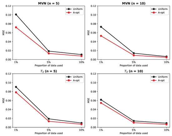
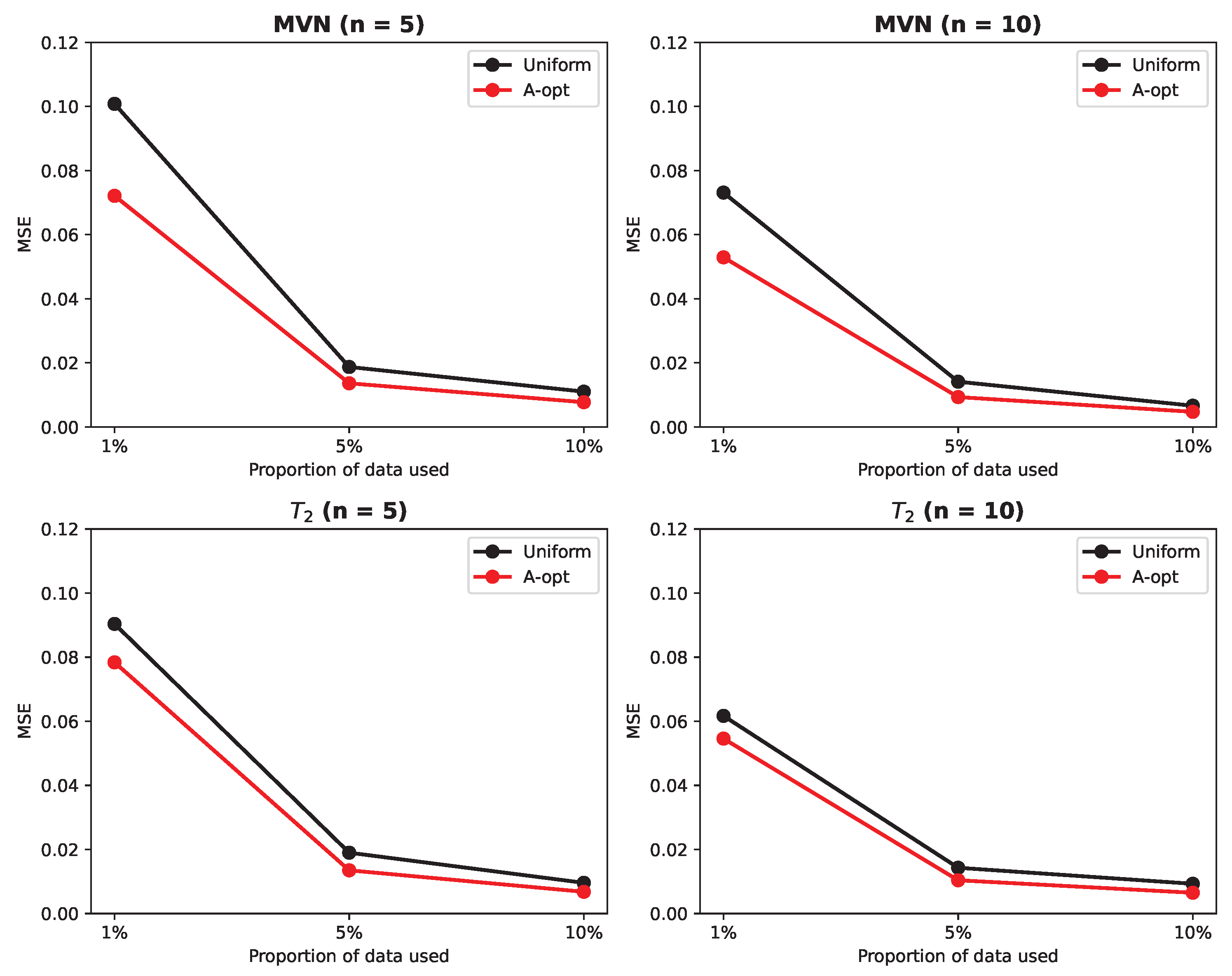
Figure 1 displays the MSEs of $\tilde{\mathit{\theta }}$ across all scenario combinations.

Figure 1. Empirical MSEs of $\tilde{\mathit{\theta }}$ under the linear mixed-effects model for uniform and optimal subsampling, across two observation-count scenarios (Scenario 1: $n\approx 5$; Scenario 2: $n\approx 10$), two covariate distributions (MVN and ${\mathbf{T}}_2$), and three subsampling fractions (1%, 5%, 10% of $m=500,000$). Each point is averaged over 500 replications.

To quantify the gain visible in Figure 1, Table 2 reports the empirical MSEs together with the relative efficiency $\mathrm{RE}={\mathrm{MSE}}_{\mathrm{uniform}}/{\mathrm{MSE}}_{A\text{-opt}}$ for each scenario combination. The relative efficiency exceeds one in every scenario, confirming that A-optimal subsampling is uniformly more accurate than uniform subsampling; across the scenarios considered, it ranges from about $1.13$ to $1.52$. In absolute terms, the MSE gap between the two methods is largest at the $1\%$ fraction, where the estimation problem is hardest, and prioritizing informative subjects matters most. The relative efficiency, by contrast, tends to be larger at the larger fractions: because both methods are accurate there, even a small absolute improvement corresponds to a sizable ratio. Taken together, Figure 1 and Table 2 show that the optimal method never does worse than uniform subsampling and yields its most pronounced absolute benefit precisely when the data budget is smallest.

Table 2. Empirical MSEs and relative efficiency $\mathrm{RE}={\mathrm{MSE}}_{\mathrm{uniform}}/{\mathrm{MSE}}_{A\text{-opt}}$ for each scenario, averaged over 500 replications.

Covariate Distribution	Subsampling Fraction	MSE		RE
		Uniform	A-opt
Scenario 1 ($n\approx 5$)
MVN	1%	0.1008	0.0721	1.3981
	5%	0.0187	0.0136	1.3750
	10%	0.0110	0.0077	1.4286
${\mathbf{T}}_2$	1%	0.0904	0.0784	1.1531
	5%	0.0190	0.0135	1.4074
	10%	0.0096	0.0068	1.4118
Scenario 2 ($n\approx 10$)
MVN	1%	0.0731	0.0529	1.3819
	5%	0.0141	0.0093	1.5161
	10%	0.0066	0.0047	1.4043
${\mathbf{T}}_2$	1%	0.0617	0.0546	1.1300
	5%	0.0143	0.0104	1.3750
	10%	0.0093	0.0065	1.4308

To quantify the computational saving that motivates the proposed method, Table 1 reports the runtime of the full-data, uniform-subsampling, and A-optimal-subsampling estimators across all scenarios using a reduced problem size, $m=50,000$, on a single machine (a Mac mini). The full simulation size $m=500,000$ could not be run to completion for the full-data estimator on this machine within a practical time frame, which illustrates the computational barrier motivating subsampling. For the timing study, each estimator was run under every scenario combination over 10 independent runs and averaged. The results show that, at $m=50,000$, the subsampling estimators require less runtime than the full-data estimator on the same machine. We therefore report the reduced-size timing study as a practical computational comparison, while noting that the inability to complete the $m=500,000$ full-data fit on the same machine is consistent with the need for subsampling in large-scale settings.

The results in Figure 1 reveal a consistent pattern across all scenarios: the optimal subsampling method attains a lower MSE than uniform subsampling, and the advantage grows as the subsampling fraction decreases. Based on these findings, we offer the following recommendations for practitioners.

1.

More observations per subject were associated with lower MSE in these scenarios. Across the simulated settings, increasing the typical number of observations per subject from approximately five (Scenario 1) to approximately ten (Scenario 2) consistently reduced the MSE of $\tilde{\mathit{\theta }}$. This suggests that, where the study design and measurement budget allow, additional repeated measurements per subject can improve the estimation accuracy; we caution, however, that our simulation does not model the practical costs of collecting more visits, so this should not be read as a blanket recommendation.

2.

Under normally distributed covariates and moderate subsampling fractions, the absolute MSE gap between uniform and optimal subsampling was small. When at least 10% of the data were used, and the covariate distribution was approximately multivariate normal, the absolute MSE gap between uniform and optimal subsampling was small in our experiments. In such settings, the simpler uniform method may be an adequate choice, though this conclusion is specific to the scenarios considered.

3.

Optimal subsampling showed the largest absolute gains when the subsampling fraction was small. When only 1% of the data were used, optimal subsampling outperformed uniform subsampling by the widest margin in the absolute MSE, and the gap narrowed as the subsampling fraction increased. In these regimes, the modest additional overhead of the two-step algorithm appears well justified; as above, this reflects the simulated scenarios rather than a general guarantee.

5. Discussion

The simulation evidence points to a consistent pattern: the heavier the tails of the covariate distribution and the smaller the subsampling fraction, the larger the advantage of optimal over uniform subsampling in terms of estimation accuracy. This finding has a natural interpretation. When covariates follow a heavy-tailed distribution, a small number of subjects with extreme covariate values carry disproportionate information about the model parameters; uniform subsampling selects such subjects only rarely, whereas the optimal probabilities, being proportional to the scaled gradient norm, steer the sample toward precisely these influential subjects. As the subsampling fraction decreases, this prioritization becomes increasingly important relative to the contribution of the remaining subjects, explaining the widening performance gap.

The proposed framework extends the A-optimal subsampling theory of Wang et al. [29] to the substantially more general setting of multivariate longitudinal data under an unbalanced design. We derived closed-form expressions for the A-optimal and L-optimal subsampling probabilities within the linear mixed-effects model and provided a practical two-step algorithm together with sandwich-type standard error estimators.

Several directions for future research are worth pursuing. First, the present framework assumes that all data are stored centrally; an important practical extension is to develop distributed subsampling algorithms suited to data partitioned across multiple servers or storage nodes. Second, we focused on the parsimonious error structure ${\mathbf{\Sigma }}_i=\mathbf{\Sigma }\otimes {\mathbf{I}}_{n_i}$; extending the framework to accommodate richer within-subject error structures, such as first-order autoregressive (AR(1)) or unstructured covariances, would broaden its applicability. We emphasize that this Kronecker specification, while parsimonious and computationally convenient, is a genuine modeling restriction: it assumes that, conditional on the random effects, the residuals are uncorrelated across time points, so that all within-subject serial dependence is absorbed by the random-effects structure. This may be inadequate for longitudinal applications in which residual autocorrelation persists after conditioning on the random effects—for example, densely or closely spaced visits—and sensitivity analyses under AR(1) or unstructured residual covariances would therefore be desirable. More generally, additional simulation studies under covariance misspecification and non-normal random-effects distributions would provide a useful robustness assessment beyond the Gaussian mixed-effects setting considered here. Third, the current asymptotic results require both $m\to \infty$ and $r\to \infty$; characterizing the finite-sample approximation error and deriving non-asymptotic bounds on the MSE would strengthen the theoretical foundations. Finally, adapting the deterministic information-based subdata selection paradigm of Wang et al. [27] to the mixed-effects setting would provide a useful complement to the random subsampling approach developed here.

References

- Verbeke, G.; Fieuws, S.; Molenberghs, G.; Davidian, M. The analysis of multivariate longitudinal data: A review. Stat. Methods Med. Res. 2014, 23, 42–59. [Google Scholar] [CrossRef] [Scilit]
- Bandyopadhyay, S.; Ganguli, B.; Chatterjee, A. A review of multivariate longitudinal data analysis. Stat. Methods Med. Res. 2011, 20, 299–330. [Google Scholar] [CrossRef] [Scilit]
- Galecki, A.T. General class of covariance structures for two or more repeated factors in longitudinal data analysis. Commun. Stat.-Theory Methods 1994, 23, 3105–3119. [Google Scholar] [CrossRef] [Scilit]
- Carey, V.J.; Rosner, B.A. Analysis of longitudinally observed irregularly timed multivariate outcomes: Regression with focus on cross-component correlation. Stat. Med. 2001, 20, 21–31. [Google Scholar] [CrossRef] [Scilit]
- Liang, K.-Y.; Zeger, S.L. A class of logistic regression models for multivariate binary time series. J. Am. Stat. Assoc. 1989, 84, 447–451. [Google Scholar] [CrossRef]
- Oort, F.J. Three-mode models for multivariate longitudinal data. Br. J. Math. Stat. Psychol. 2001, 54, 49–78. [Google Scholar] [CrossRef] [Scilit] [PubMed]
- McArdle, J.J. Dynamic but Structural Equation Modeling of Repeated Measures Data; Springer: Boston, MA, USA, 1988; pp. 561–614. ISBN 978-1-4613-0893-5. [Google Scholar] [CrossRef] [Scilit]
- Duncan, S.C.; Duncan, T.E. A multivariate latent growth curve analysis of adolescent substance use. Struct. Equ. Model. A Multidiscip. J. 1996, 3, 323–347. [Google Scholar] [CrossRef] [Scilit]
- Laird, N.M.; Ware, J.H. Random-effects models for longitudinal data. Biometrics 1982, 38, 963–974. [Google Scholar] [CrossRef] [Scilit] [PubMed]
- Chakraborty, H.; Helms, R.W.; Sen, P.K.; Cohen, M.S. Estimating correlation by using a general linear mixed model: Evaluation of the relationship between the concentration of hiv-1 rna in blood and semen. Stat. Med. 2003, 22, 1457–1464. [Google Scholar] [CrossRef] [Scilit] [PubMed]
- Yang, X.; Chen, J.; Li, D.; Li, R. Functional-coefficient quantile regression for panel data with latent group structure. J. Bus. Econ. Stat. 2024, 42, 1026–1040. [Google Scholar] [CrossRef] [Scilit] [PubMed]
- Zhou, Z.; Wang, Y.; Liu, X.; Li, Z.; Wu, M.; Zhou, G. Hybrid of neural network and physics-based estimator for vehicle longitudinal dynamics modeling using limited driving data. IEEE Trans. Intell. Transp. Syst. 2025, 26, 16735–16746. [Google Scholar] [CrossRef] [Scilit]
- Chen, J.; Li, L.; Wang, Y.; Zhang, Q.; Chen, H.; Zhou, J.; Wu, M. Direct data-driven trajectory tracking control for autonomous vehicles via algebraic regulator under limited data. IEEE Trans. Ind. Inform. 2026. Advance online publication. [Google Scholar] [CrossRef] [Scilit]
- Drineas, P.; Mahoney, M.W.; Muthukrishnan, S. Sampling algorithms for l2 regression and applications. In Proceedings of the 17th Annual ACM-SIAM Symposium on Discrete Algorithms, Miami, FL, USA, 22–24 January 2006; pp. 1127–1136. [Google Scholar]
- Ma, P.; Mahoney, M.W.; Yu, B. A statistical perspective on algorithmic leveraging. J. Mach. Learn. Res. 2015, 16, 861–991. [Google Scholar]
- Yang, T.; Zhang, L.; Jin, R.; Zhu, S. An explicit sampling dependent spectral error bound for column subset selection. In Proceedings of the 32nd International Conference on Machine Learning; Bach, F., Blei, D., Eds.; PMLR: Cambridge, MA, USA, 2015; Volume 37, pp. 135–143. Available online: https://proceedings.mlr.press/v37/yanga15.html (accessed on 3 March 2022).
- Drineas, P.; Magdon-Ismail, M.; Mahoney, M.W.; Woodruff, D.P. Fast approximation of matrix coherence and statistical leverage. J. Mach. Learn. Res. 2012, 13, 3475–3506. [Google Scholar]
- Zhu, R. Gradient-based sampling: An adaptive importance sampling for least-squares. In Advances in Neural Information Processing Systems; Curran Associates Inc.: Red Hook, NY, USA, 2016; Volume 29, pp. 406–414. [Google Scholar]
- Wang, H.Y.; Zhu, R.; Ma, P. Optimal subsampling for large sample logistic regression. J. Am. Stat. Assoc. 2018, 113, 829–844. [Google Scholar] [CrossRef] [Scilit] [PubMed]
- Yao, Y.; Wang, H.Y. Optimal subsampling for softmax regression. Stat. Pap. 2019, 60, 235–249. [Google Scholar]
- Ai, M.; Yu, J.; Zhang, H.; Wang, H.Y. Optimal subsampling algorithms for big data regressions. Stat. Sin. 2021, 31, 749–772. [Google Scholar] [CrossRef] [Scilit]
- Lee, J.; Schifano, E.D.; Wang, H.Y. Fast optimal subsampling probability approximation for generalized linear models. Econom. Stat. 2021, 29, 224–237. [Google Scholar] [CrossRef] [Scilit]
- Ai, M.; Wang, F.; Yu, J.; Zhang, H. Optimal subsampling for large-scale quantile regression. J. Complex. 2021, 62, 101512. [Google Scholar] [CrossRef] [Scilit]
- Wang, H.Y.; Ma, Y. Optimal subsampling for quantile regression in big data. Biometrika 2021, 108, 99–112. [Google Scholar] [CrossRef] [Scilit]
- Yu, J.; Wang, H.Y.; Ai, M.; Zhang, H. Optimal distributed subsampling for maximum quasi-likelihood estimators with massive data. J. Am. Stat. Assoc. 2022, 117, 265–276. [Google Scholar] [CrossRef] [Scilit]
- Wang, J.; Zou, J.; Wang, H.Y. Sampling with replacement vs poisson sampling: A comparative study in optimal subsampling. IEEE Trans. Inf. Theory 2022, 68, 6605–6630. [Google Scholar] [CrossRef] [Scilit]
- Wang, H.Y.; Yang, M.; Stufken, J. Information-based optimal subdata selection for big data linear regression. J. Am. Stat. Assoc. 2019, 114, 393–405. [Google Scholar]
- Pronzato, L.; Wang, H.Y. Sequential online subsampling for thinning experimental designs. J. Stat. Plan. Inference 2021, 212, 169–193. [Google Scholar] [CrossRef] [Scilit]
- Wang, Z.; Wang, H.Y.; Ravishanker, N. Subsampling in longitudinal models. Methodol. Comput. Appl. Probab. 2023, 25, 35. [Google Scholar] [CrossRef] [Scilit]
- Xie, R.; Wang, Z.; Bai, S.; Ma, P.; Zhong, W. Online decentralized leverage score sampling for streaming multidimensional time series. In Proceedings of the Twenty-Second International Conference on Artificial Intelligence and Statistics; Chaudhuri, K., Sugiyama, M., Eds.; PMLR: Cambridge, MA, USA, 2019; Volume 89, pp. 2301–2311. Available online: https://proceedings.mlr.press/v89/xie19a.html (accessed on 3 March 2022).
- Lindstrom, M.J.; Bates, D.M. Newton-raphson and em algorithms for linear mixed-effects models for repeated-measures data. J. Am. Stat. Assoc. 1988, 83, 1014–1022. [Google Scholar] [CrossRef] [Scilit]
- van der Vaart, A. Asymptotic Statistics; Cambridge University Press: Cambridge, UK, 1998. [Google Scholar]
Disclaimer/Publisher’s Note: The statements, opinions and data contained in all publications are solely those of the individual author(s) and contributor(s) and not of MDPI and/or the editor(s). MDPI and/or the editor(s) disclaim responsibility for any injury to people or property resulting from any ideas, methods, instructions or products referred to in the content. |
© 2026 by the authors. Licensee MDPI, Basel, Switzerland. This article is an open access article distributed under the terms and conditions of the Creative Commons Attribution (CC BY) license.