


Abstract
Identifying the most appropriate lag structure for double seasonal autoregressive models is a fundamental demanding task in time series analysis. Classical model selection tools such as the Akaike information criteria are well known to be inconsistent for identifying the true lag structure. At the same time, standard Bayesian formulations almost invariably assume normality that is often violated in the presence of heavy tails, isolated outliers, or contaminated observations. This paper addresses both limitations simultaneously by proposing a unified Bayesian framework for the best-subset selection of multiplicative double seasonal autoregressive models under the scale-mixtures of normal family of error distributions. Adopting an extended stochastic search variable selection, we assign mixture-normal priors to all primitive autoregressive coefficient vectors and derive tractable closed-form conditional posterior distributions for all model parameters. Building on these results, we design an efficient Markov chain Monte Carlo algorithm integrating Gibbs sampling and Metropolis–Hastings updates for simultaneous subset identification and parameter estimation under heavy-tailed errors. A comprehensive simulation study and real-data applications to hourly electricity demand in the Czech Republic and Germany demonstrate that the proposed algorithm consistently outperforms classical information criteria, particularly when innovations are heavy-tailed.
Keywords:
DSAR models; electricity demand; Gibbs sampler; heavy-tailed errors; MCMC methods; Metropolis–Hastings algorithm; SMN distributions; SSVS procedure MSC:
62M10; 62F15
1. Introduction
Time series exhibiting double seasonality arise naturally across a broad range of application domains. The most prominent instance is high-frequency energy data; i.e., hourly electricity demand oscillates within each day and simultaneously across the week, manifesting both a 24 h intraday cycle and a 168 h weekly cycle [1]. Related phenomena appear in telecommunications traffic, retail sales, and transportation flow data. All of these cases require modelling frameworks capable of capturing the complex interaction between short-term and long-term seasonal cycles. Among available parametric tools, the multiplicative double seasonal autoregressive (DSAR) model [2,3,4] provides a principled and parsimonious representation of such dynamics. By factoring the DSAR operator into three polynomial components, the model encodes additive effects from individual lags alongside their pairwise and triple interaction terms. This model faithfully preserves the genuinely multiplicative structure inherent in many periodic phenomena.
This structural richness, however, comes at a price. The practitioner must determine, for each of the three autoregressive (AR) polynomials, which specific lags carry meaningful signal and which should be omitted. When the DSAR maximum orders p, P, and Q are set conservatively, as is necessary when the true structure is unknown, the candidate space comprises distinct subsets. Exhaustive search over this space becomes rapidly prohibitive even for moderate maximum orders, and a principled yet computationally feasible method for navigating it is therefore essential. Classical information-criterion-based strategies, such as the Akaike information criterion (AIC) [5] and the corrected AIC [6], are widely applied in practice but are known to be inconsistent estimators of the true lag structure. Their selection accuracy does not converge to one as the sample size grows [7]. Moreover, these frequentist criteria evaluate each candidate model independently, making them computationally expensive and unable to quantify uncertainty about the selected structure.
The stochastic search variable selection (SSVS) procedure introduced by George and McCulloch [8] provides a coherent Bayesian alternative. The SSVS associates a binary indicator with each AR coefficient and assigns a two-component mixture-normal prior conditional on that indicator. This setup allows a single Markov chain Monte Carlo (MCMC) run to traverse the entire model space, yielding posterior probabilities for all subsets without fitting each model separately. This procedure is consistent, scales naturally to high-dimensional problems, and delivers genuine uncertainty quantification about the selected structure [2]. SSVS was first applied to subset selection of standard AR models by Chen [9], extended to AR models with exogenous variables and GARCH errors by So et al. [10], and adapted to threshold autoregressive moving-average structures by Chen et al. [11]. Most recently, Amin [2], Amin et al. [7] tailored SSVS to seasonal autoregressive (SAR) and DSAR models under the normality assumption, demonstrating substantial improvements over AIC in simulation experiments. The extension of SSVS-based subset selection to DSAR models under heavy-tailed errors has not been addressed in the existing literature.
The Gaussian error assumption imposed in all existing DSAR subset-selection methods is both statistically convenient and empirically fragile. For instance, high-frequency energy load series are punctuated by sudden demand spikes arising from extreme weather events, public holidays, and load-management interventions. Also, financial and economic time series routinely exhibit leptokurtosis from volatility clustering and structural breaks [12]. In all such cases, fitting a Gaussian model inflates the estimated error variance, which in turn biases the posterior inclusion probabilities of the SSVS latent indicators and degrades subset-selection accuracy.
The family of scale-mixtures of normal (SMN) distributions [13,14] provides a principled and flexible remedy. Every SMN distribution is obtained by multiplying the Gaussian variance by a positive latent mixing variable, whose marginal distribution governs the heaviness of the resulting tail. The family subsumes the Student-t, slash, and contaminated normal distributions as special cases, with the standard Gaussian arising as a limiting case [15]. This rich hierarchy provides several critical advantages. First, conditioning on the latent mixing variables restores local Gaussianity at each observation. This preserves the conjugacy that makes the conditional posteriors of DSAR parameters analytically tractable. Second, the observation-specific mixing values act as automatic outlier down-weighting factors. Observations with small mixing values are flagged as potential outliers and receive reduced influence in the posterior, protecting the subset-selection probabilities from distortion [16,17]. Third, the SMN framework admits a straightforward hierarchical representation that dovetails seamlessly with Gibbs-sampling schemes [18].
The relevance of SMN errors for Bayesian analysis of time series models has been demonstrated in a growing body of work. Ferreira et al. [19] presented a Bayesian approach for partial linear models featuring AR(1) errors drawn from an SMN distribution. Maleki and Nematollahi [20] derived key theoretical results for AR processes with SMN innovations and introduced an EM algorithm for estimation. Building on this line of work, Amin [21,22,23] proposed Bayesian estimation, forecasting, and comprehensive analysis for seasonal AR models under SMN error structures.
By simultaneously tackling the limitations of classical information criteria and the fragility of the normal-errors specification under heavy-tailed data, we develop an MCMC-driven Bayesian framework for DSAR model selection with SMN errors. The present work makes the following original contributions.
- We extend SSVS to accommodate SMN errors in multiplicative DSAR models by augmenting the model with the mixing-variable vector, which preserves conjugacy and renders all conditional posteriors analytically tractable.
- We obtain closed-form expressions for the full conditional posteriors of the DSAR coefficients and the scale parameter, as well as for the mixing weights and shape parameters, identifying which require Metropolis–Hastings updates.
- We construct an efficient MCMC algorithm integrating Gibbs sampling, Metropolis–Hastings updates, and SSVS for simultaneous identification and estimation under heavy-tailed errors.
- We conduct an extensive simulation study spanning four DSAR configurations with distinct SMN error distributions and compare against AIC and corrected AIC. We further apply the methodology to hourly electricity demand data from the Czech Republic and Germany.
The subsequent sections of the paper are arranged as follows. Section 2 reviews the SMN distribution and specifies the DSAR model. Section 3 introduces the prior distributions and derives the augmented joint posterior. Section 4 contains the main theoretical results for the conditional posteriors of DSAR models. The MCMC algorithm for the Bayesian subset selection of DSAR models is described in Section 5. Section 6 reports the simulation study and real-data application. Section 7 concludes the paper.
2. DSAR Models Under Scale-Mixtures of Normal Errors
2.1. Scale-Mixtures of Normal Distribution
Definition 1 (SMN Distribution).
A random variable y follows a scale-mixture of normal (SMN) distribution with location μ and scale if it admits the hierarchical stochastic representation
where is a positive latent random variable with density indexed by hyperparameter (scalar or vector-valued), and ε is independent of κ.
We write when representation (1) holds. The four SMN cases considered in this paper are as follows:
- SMN-n (Normal): ; i.e., is degenerate at unity, recovering the standard Gaussian distribution.
- SMN- (Student-): with . The marginal distribution of y is Student-t with degrees of freedom, with the Cauchy distribution arising at .
- SMN-sl (Slash): restricted to with . The marginal is the slash distribution with shape , exhibiting heavier tails than the Student-t for small values of [24].
- SMN-cn (Contaminated Normal): is discrete, taking value with probability and value 1 otherwise:modelling a scenario in which a proportion of observations are variance-inflated (contaminated) while the rest follow the standard Gaussian [25].
The SMN family is especially suited to robust Bayesian inference because conditioning on the latent variables restores local Gaussianity [15,17], a property that is central to the tractable derivations in Section 4.
2.2. DSAR Model Specification and Notation
Let be a zero-mean, stationary time series with two distinct seasonal periods . We say that follows a multiplicative DSAR model of nonseasonal order p, first seasonal order P (period ), and second seasonal order Q (period ), denoted , if
where B is the backshift operator () and the three autoregressive polynomials are
The vectors , , and collect the nonseasonal, first-seasonal, and second-seasonal primitive AR coefficients, respectively. The errors are independently distributed from an SMN distribution with location zero and scale .
Expanding the product in (3) yields
where is the extended regressor vector of lagged observations and is the expanded coefficient vector encoding the primitive coefficients , , together with all their pairwise and triple multiplicative interactions. The full structure of and is detailed in Amin [2], and the dimension of is .
Stacking the n equations gives
where , , and is the design matrix whose t-th row is . The multiplicative structure of renders the DSAR model nonlinear in the primitive parameters , , and . Even the marginal posterior distributions of these parameters are therefore analytically intractable, motivating the MCMC approach developed in Section 4 and Section 5.
Stationarity of the process requires that all roots of the three AR characteristic polynomials , , and lie strictly outside the unit circle. Because the Gaussian-mixture priors placed on , , and have full support over , , and respectively, the posterior sampler can, in principle, generate draws that violate stationarity. To ensure that the MCMC chain remains in the stationary region, we adopt a three-pronged strategy. First, the observed series is pre-processed via appropriate differencing and/or seasonal adjustments to induce stationarity prior to Bayesian analysis. Second, the ordinary least squares (OLS) estimates are used to initialize the sampler; in the simulation studies these starting values are stationary because the true data-generating parameters lie well inside the stationarity region. Third, after each Gibbs update of (), we compute the modulus of all roots of the associated polynomial and reject any draw that produces at least one root inside or on the unit circle. This reflection step imposes the stationarity constraint while adding negligible computational cost, as non-stationary draws become rare once the chain has converged near the posterior mode. This approach combines standard data transformation, careful initialization, and explicit post-draw rejection to maintain theoretical validity and sampling efficiency.
Under the SMN specification, conditioning on the latent mixing variables gives
Denoting and , the augmented log-likelihood of is given:
Intuitively, from the augmented log-likelihood (10), each observation in an SMN model carries its own local variance weight . For a typical observation and the model behaves like a Gaussian; for an outlier, inflates the local variance so the residual contributes little to the likelihood and therefore little to the posterior of the AR coefficients. This automatic down-weighting protects the lag-inclusion probabilities from being distorted by a handful of extreme values—a practically important property for data containing spikes or extreme values [16,17].
3. Bayesian Framework for Subset Selection Under SMN Errors
Following the SSVS paradigm of George and McCulloch [8], we associate a binary latent indicator with each primitive AR coefficient, encoding whether the corresponding lag is retained in the model. Specifically, we define three latent-indicator vectors parallel to the three AR coefficient vectors:
These are collected into vectors , , and , which govern the inclusion of lags in , , and , respectively.
We specify the mixture-normal priors for the primitive AR coefficients. The prior on each coefficient conditional on its indicator takes the two-component mixture form:
where is a small prior variance that penalises inactive coefficients toward zero (when ), and ensures that active coefficients (when ) can attain non-negligible magnitudes, consistent with the original SSVS prescription of George and McCulloch [8].
Conditionally on the indicator vectors, the joint priors over the three AR coefficient vectors are multivariate normal:
where () is the diagonal scaling matrix
with if and if (here, , , ), and is a prior correlation matrix for the i-th AR vector, typically taken to be the identity matrix .
In addition, we specify the inverse-gamma prior for the scale parameter:
where and are fixed hyperparameters. Diffuse choices are standard when no prior information is available.
We employ Bernoulli priors for the latent indicator variables. The indicators within each vector are assumed a priori independent, with inclusion probabilities , , and . The joint indicator priors are
The uniform special case assigns equal prior probability to inclusion and exclusion of every lag.
Regarding the prior specification of SMN hyperparameters, the prior depends on the specific SMN member. Following Cabral et al. [18],
- SMN-: truncated to , with , .
- SMN-sl: Same as SMN-t but truncated to .
- SMN-cn: and , all hyperparameters strictly positive.
Let denote the full augmented parameter vector. Assuming a priori independence between the SMN hyperparameters and the remaining parameters, the joint prior factorises as
Combining (10) with (25) via Bayes’ theorem yields the augmented joint posterior:
This joint posterior is nonlinear in , , through the expanded vector , which prevents direct marginalisation. The conditional posteriors required for the MCMC algorithm are derived in the next section.
4. Conditional Posterior Distributions
To facilitate the MCMC algorithm, we reformulate the DSAR model (8) in three alternative linear decompositions that isolate each primitive AR vector while holding the other two fixed. Expanding the multiplicative structure of (7) and rearranging, we obtain the linear decompositions isolating (for each ):
Particularly, for , grouping in (7) all terms multiplied by ,
Every pairwise product and triple product contributes to the i-th column of (with and treated as fixed constants), while the pure products are absorbed into . No cross-terms in are omitted, so the conditional kernel is exactly quadratic in . The same argument applies for by symmetry, where , and depend on the primitive AR vector . is an matrix with the -element,
is an matrix with the -element,
is an matrix with the -element,
and is the matrix collecting the columns of associated with , the complementary -vector of the remaining two primitive AR vectors concatenated (where , , ). These matrices are fully constructed and presented in Amin [2]. These three decompositions are exact. Every cross-product term is absorbed into the complementary offset vector when the other two AR vectors are held fixed at their current MCMC values.
4.1. Conditional Posteriors of the DSAR Coefficient Vectors and Scale Parameter
Theorem 1
(Conditional posterior of ). The full conditional posterior distribution of the DSAR coefficients vector , for each , given all other parameters and the data, is multivariate normal of dimension (where , , ):
where and are and respectively:
Proof.
Theorem 1 shows that each of the three primitive AR vectors has a multivariate normal conditional posterior regardless of the SMN member chosen. The SMN mixing variables enter exclusively through the weighted information matrices . Observations with small are automatically down-weighted, reducing their influence on the conditional mean and providing inherent outlier robustness [15]. When (the Gaussian case), this theorem reduces precisely to the normal-errors results of Amin [2].
4.2. Conditional Posterior of the Scale Parameter
Theorem 2
(Conditional posterior of ). The full conditional posterior of , given all other parameters and the data, is inverse-gamma:
where
and denotes the residual vector.
Proof.
Retaining only the terms in (26) that involve ,
which is the kernel of . □
4.3. Conditional Posteriors of the Latent Indicator Variables
Theorem 3
(Conditional posteriors of , ). The full conditional posterior of each indicator , for and the appropriate range of j, given all other parameters and the data, is Bernoulli:
where
and denotes the prior density of under indicator value d, evaluated at the current MCMC draw of .
Proof.
Fix all parameters except . The full conditional of is proportional to
where is the prior density of , evaluated at the current MCMC value of . This is the Rao–Blackwellised SSVS update of George and McCulloch [8], George and McCulloch [26]. The likelihood has already been incorporated into the current draw of , so evaluating the prior density here introduces no double-counting. The prior density is the multivariate normal in (17)–(19) with the j-th diagonal element of set to if and if , while all other diagonal elements remain at their current values. Evaluating at and normalising yields the Bernoulli probability stated. □
The quantities and are evaluated by computing the multivariate normal prior density at and , respectively, with all other parameters held at their current MCMC values. This is standard SSVS practice [8,26,27].
4.4. Conditional Posteriors of the SMN Mixing Variables and Hyperparameters
In the following, we obtain the conditional posteriors of and to each non-Gaussian SMN member. Let be the t-th residual.
- Conditional posteriors under SMN-t.
Under the Student-t parameterisation with :
- 1.
- Each mixing variable: , .
- 2.
- The degrees-of-freedom parameter has a non-standard conditional densitywhich is sampled via a Metropolis–Hastings step using a truncated-normal proposal centred at the current with variance equal to the negative reciprocal of .
- 3.
- The exponential rate hyperparameter: .
- Conditional posteriors under SMN-sl.
- Under the slash parameterisation with :
- 1.
- Each mixing variable: .
- 2.
- The slash shape parameter: .
- 3.
- The hyperparameter: .
- Conditional posteriors under SMN-cn.
- Under the contaminated-normal parameterisation:
- 1.
- Each mixing variable is discrete:where and .
- 2.
- The contamination proportion: , where . Because each has already been sampled as a fixed draw in Step 1 above, the conditional posterior of given is an augmented-data full conditional, not a marginal or partially collapsed one. Retaining only terms involving , for those t with the contribution is , and for those with the factor is constant in and cancels. Combined with the Beta prior, the full conditional density iswhich is sampled via a Metropolis–Hastings step using a log-normal proposal .
A natural concern is whether the observation-specific scale variables may absorb serial dependence that should instead be attributed to additional AR lags, thereby distorting subset-selection probabilities. Identifiability is ensured by the following structural argument. The mixing variables are observation-specific and mutually independent given ; they scale the innovation variance at time t but do not alter the conditional mean . The AR lag structure is identified through the conditional mean, which depends on , , regardless of . Hence, outlier down-weighting via and lag inclusion via operate on orthogonal components, i.e., the conditional variance and the conditional mean, respectively, and their posteriors are updated in separate Gibbs blocks.
5. MCMC Algorithm for Bayesian Subset Selection of DSAR Models
The conditional posteriors derived in Section 4, taken together, constitute the complete set of distributions required to introduce an MCMC algorithm for simultaneous subset selection and parameter estimation in DSAR models under SMN errors. The complete MCMC algorithm is specified in Algorithm 1.
| Algorithm 1: MCMC Algorithm for Bayesian Subset Selection of under SMN Errors. |
|
The algorithm is initialised by obtaining starting values from fitting the full model by nonlinear ordinary least squares [2,32]. All latent indicators are initialised at unity (full model), all mixing variables at , and the SMN hyperparameter at its prior mean. After completing iterations and applying burn-in and thinning, the best-subset DSAR model is identified as the triple attaining the highest posterior frequency among the retained draws. Ties are resolved by consulting the 95% credible intervals of the corresponding primitive coefficients [27]. As a complementary uncertainty summary we report the marginal posterior inclusion probability for each primitive lag, , whose Monte Carlo standard error is .
Algorithm 1 reduces to the normal-errors Bayesian subset selection algorithm of Amin et al. [7] when SMN-n is adopted (, SMN updates omitted), and further to the Gaussian DSAR analysis of Amin [2] when the indicators are all fixed at unity (no selection). These nested special cases provide useful consistency checks.
The initial iterations are discarded to eliminate the influence of starting values, and the remaining chain is thinned by retaining every -th draw to reduce autocorrelation [28,33]. Satisfactory convergence is declared when all of the following hold simultaneously: (a) Geweke’s Z-statistic [29] is below 1.96 in absolute value for every scalar parameter (indicating no significant difference between the first 10% and last 50% of the chain at the 5% level); (b) the Raftery–Lewis diagnostic [30] recommends a chain length not exceeding the number of draws actually used; and (c) empirical autocorrelations of the thinned chains are also inspected; rapid decay to near-zero by lag 10 indicates negligible residual dependence [31].
Regarding computational cost, each iteration of Algorithm 1 requires: (i) Bernoulli draws for the indicators (negligible); (ii) three multivariate normal draws of dimensions p, P, and Q, each dominated by an Cholesky factorisation of ; (iii) an inverse-gamma draw and n independent scalar draws for the mixing variables, both ; and (iv) at most two Metropolis–Hastings steps of cost each. Scalability to larger orders or longer series can be improved by parallelising the n mixing-variable draws across cores. When SMN-n is adopted, the mixing-variable block is dropped entirely, reducing per-iteration cost by approximately 20% for large n.
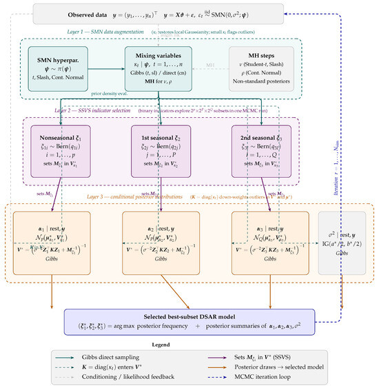
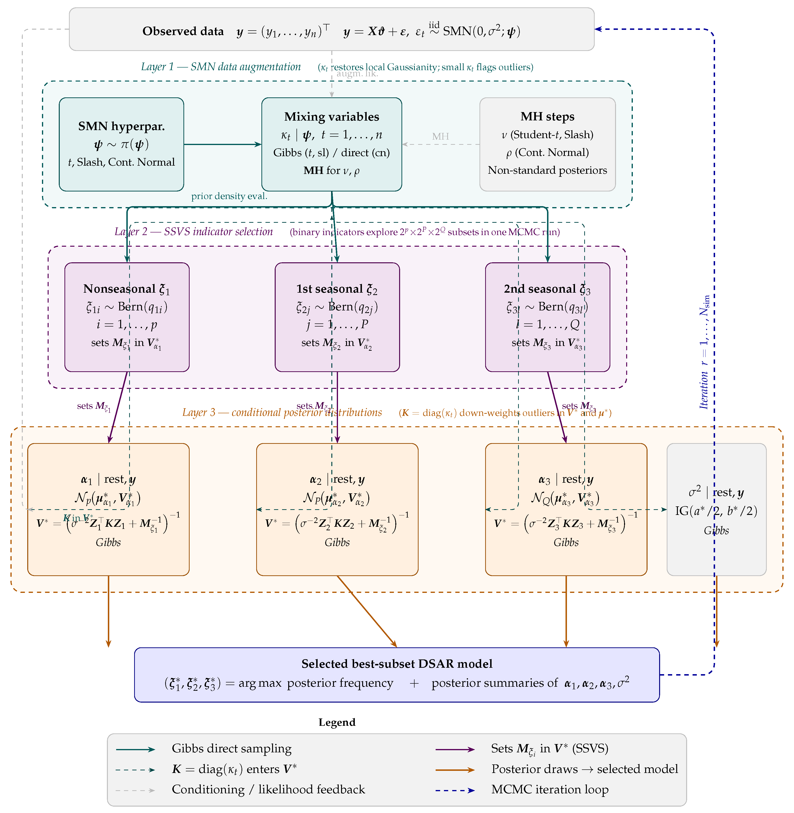
Figure 1 provides a unified schematic of the proposed Bayesian DSAR–SSVS–SMN framework, synthesising the model specification of Section 2, the prior structure and joint posterior of Section 3, and the conditional posteriors and MCMC algorithm of Section 4 and Section 5. The diagram is organised into three nested layers. Layer 1 (teal) represents the SMN data-augmentation step. The hyperparameter and the chosen SMN family jointly determine the mixing variables , which are sampled by Gibbs for the Student-t and slash cases and by direct draw for the contaminated-normal case; the degrees-of-freedom parameter and contamination scale require Metropolis–Hastings steps due to their non-standard conditional posteriors. Layer 2 (purple) represents the SSVS indicator update. Each feeds a Rao–Blackwellised Bernoulli draw for the three indicator vectors , , , which in turn set the diagonal scaling matrices in the prior covariance of each AR coefficient vector. Layer 3 (coral) represents the conditional posterior distributions of the primitive AR vectors and the scale parameter. Each is sampled directly by the Gibbs sampler, and the matrix enters the posterior precision of every AR vector, automatically down-weighting outlying observations. The entire three-layer update constitutes one MCMC iteration, repeated times as indicated by the loop arrow on the right. The output node at the bottom identifies the best-subset model as the highest-frequency indicator triplet among retained draws, together with the corresponding posterior summaries of all model parameters.
Figure 1.
Schematic of the Bayesian DSAR–SSVS–SMN framework. Three nested layers correspond to the three hierarchical components of the model.
6. Simulation Study and Real-Data Applications
6.1. Simulation Study
To evaluate the accuracy and robustness of Algorithm 1, we generate observations from four model configurations with seasonal periods and , each under a distinct SMN error distribution. The true parameter settings are reported in Table 1. For each model, 1000 independent time series of length are generated. The MCMC Algorithm 1 is applied with maximum lag orders , so the algorithm searches over candidate subsets. The algorithm runs for iterations with and , yielding 1000 posterior draws per dataset.
Table 1.
True parameter values and model structures for the simulation study (, , , 1000 replications per model).
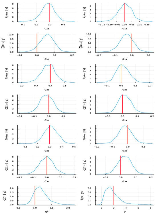
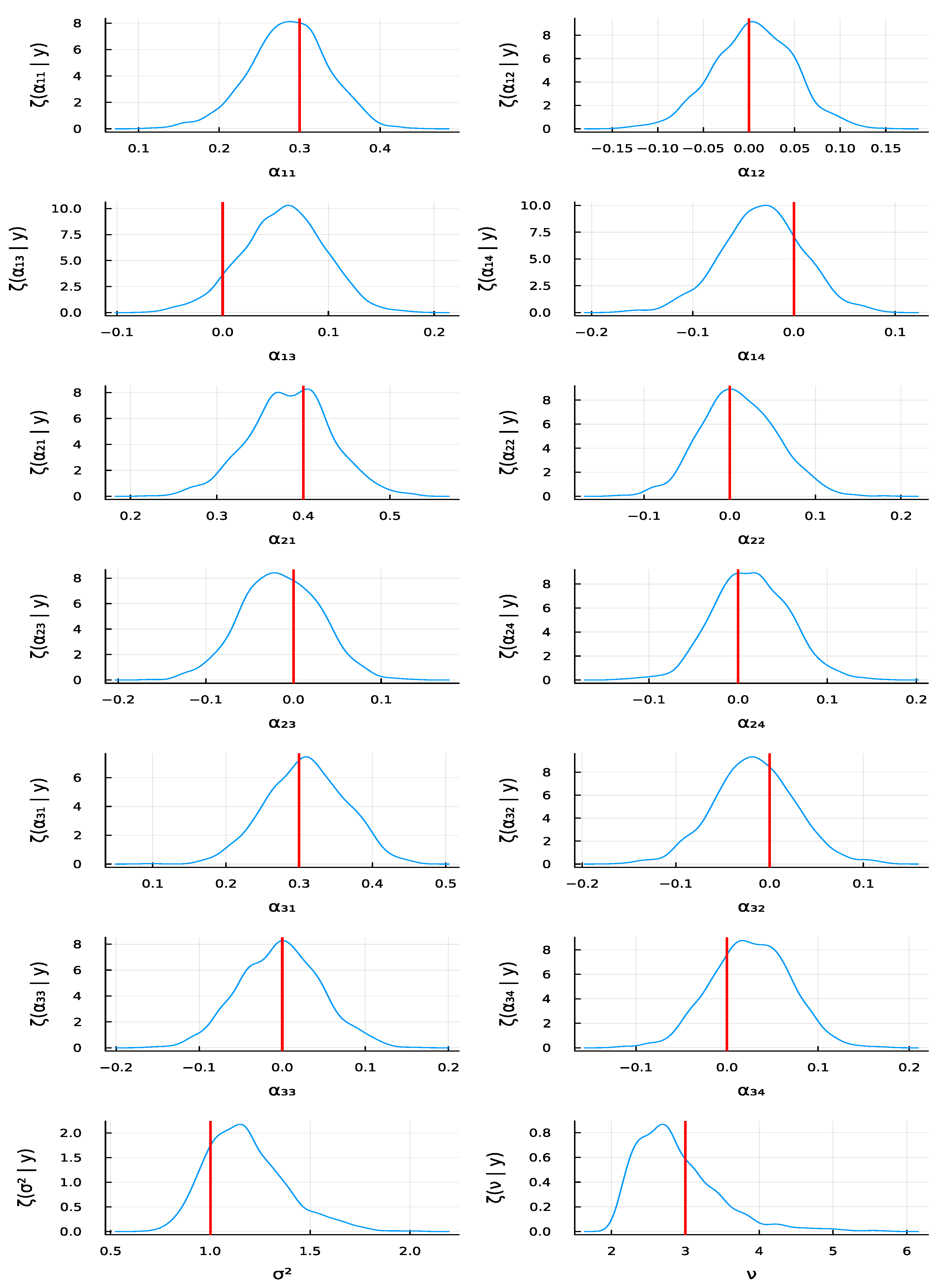
Before presenting aggregated outcomes, we illustrate the algorithm on a single realisation of Model I (, SMN-t, ). Table 2 reports the posterior frequencies of the ten most frequently visited latent-indicator triplets among the 1000 retained draws. The true configuration—corresponding to and represented by , , —attains a posterior frequency exceeding 32%, clearly identifying the correct structure. In addition, we report the posterior inclusion probabilities (PIP) and their Monte Carlo standard errors of latent-indicators in Table 3. From this table, the truly active lags all have marginal posterior inclusion probabilities above 0.95, whereas the inactive lags remain below 0.15, with Monte Carlo standard errors no larger than 0.011. Table 4 reports the Bayesian estimates of the primitive DSAR parameters, and Figure 2 displays the posterior densities of these parameters. All 95% credible intervals cover the true values, and the estimate of is consistent with the generating value, as evidenced by the vertical red lines drawn across the marginal posterior plots.
Table 2.
Posterior frequencies of latent-indicator triplets for one dataset from Model I (, SMN-t, ).
Table 3.
Posterior inclusion probabilities () and their Monte Carlo standard errors () of latent-indicators for one dataset from Model I (, SMN-t, ).
Table 4.
Bayesian estimates for one Model I dataset (, SMN-t, ). : Posterior mean; : posterior SD; : 95% credible interval.
Figure 2.
Posteriors of parameters for a single Model I-simulated time series.
Table 5 reports the percentage of correctly identified best-subset DSAR models across 1000 replications for each generating model. The proposed MCMC-based Bayesian algorithm is compared under four SMN error specifications against standard AIC and corrected AIC () measures. Recall that given a fitted model with k free parameters and maximised log-likelihood , the Akaike information criterion (AIC) is [5], and its small-sample correction is [6], where n is the sample size. Both criteria select the model minimising the respective statistic.
Table 5.
Percentage of correctly identified best-subset DSAR models across 1000 replications. Bold entries indicate the SMN specification matching the true data-generating distribution.
Table 6 summarises the aggregated posterior estimates under the correctly specified SMN error distribution, averaged across 1000 replications.
Table 6.
Aggregated Bayesian estimation results across 1000 replications under the correctly specified SMN error distribution. Active parameters only. : Mean of posterior means; : mean of posterior SDs; : mean 95% CI bounds.
The simulation results yield several clear conclusions. First, all four SMN specifications of the proposed Bayesian algorithm substantially outperform AIC and in correct subset identification, with minimum accuracy never falling below 86.7% across 1000 replications, confirming the consistency advantage of the SSVS approach. Second, the algorithm variant that correctly specifies the true error distribution consistently achieves the highest selection accuracy, outperforming the normal-errors variant when data are genuinely heavy-tailed. Third, employing a heavier-tailed SMN member when the data are in fact Gaussian incurs at most a marginal accuracy loss, confirming the practical robustness of the SMN framework. Fourth, the aggregated posterior estimates in Table 6 are highly accurate across all four scenarios, with posterior means closely tracking the true values and 95% credible intervals that consistently cover them. Fifth, marginal posterior inclusion probabilities for truly active lags exceed 0.90 on average, while those for truly inactive lags remain below 0.16, confirming that the SSVS indicators are sharply identified and not distorted by the scale-mixing component.
Convergence of the MCMC chain for one Model I dataset is formally verified by different diagnostics reported in Table 7. All Geweke z-scores lie within , confirming that the chain means in the first 10% and last 50% of the post-burn-in draws are statistically indistinguishable. The Raftery–Lewis diagnostic [30] applied to the same chain recommends a total chain length of fewer than 1000 iterations for all parameters, confirming that our is conservative. Empirical lag-10 autocorrelations of the thinned chain are below 0.05 in absolute value for all parameters. Across all 1000 replications and all simulation models, all MCMC chains pass the convergence diagnostics, verifying that the reported Bayesian selection of DSAR models are based on converged chains. Regarding the performance of this MCMC algorithm, each full run completes in approximately 8 s per dataset, for this simulation setting (, , ), on a standard laptop (Intel Core i7, 16 GB RAM, Julia 1.11.4).
Table 7.
Convergence diagnostics of the MCMC chain for one Model I dataset (, SMN-t, ).
6.2. Real-Data Applications: Hourly Electricity Demand
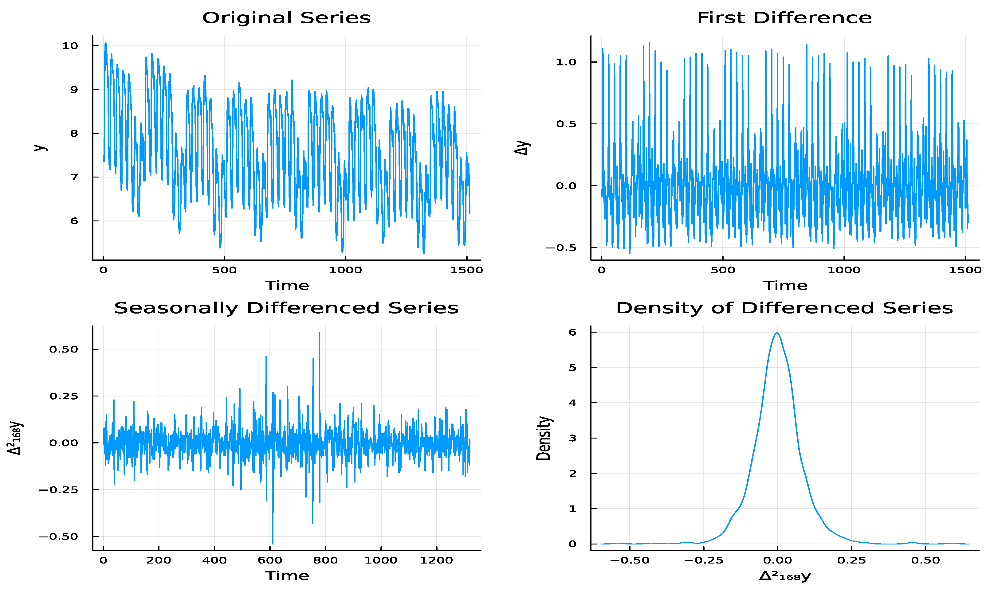
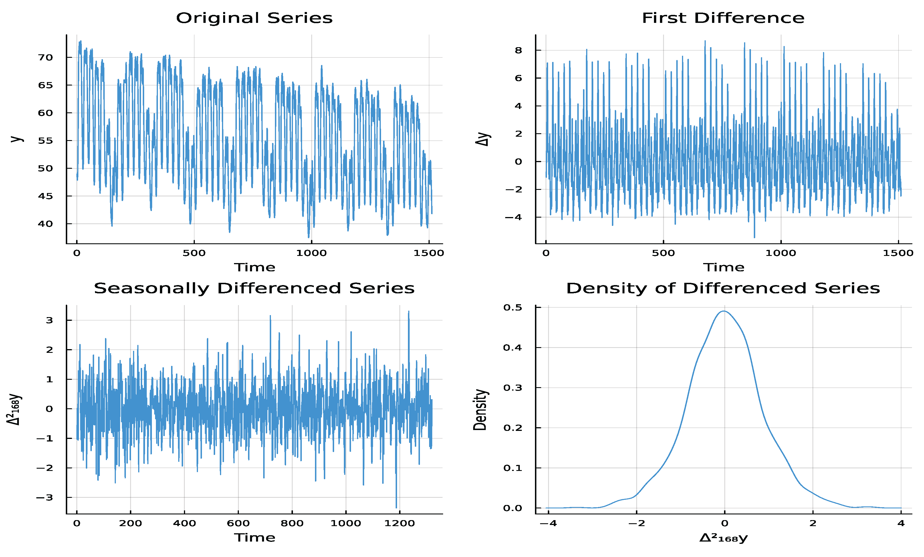
We apply the proposed methodology to hourly electricity load data from the Czech Republic and Germany, each comprising nine consecutive weeks of hourly measurements beginning on Monday, 22 January 2024. Both series simultaneously exhibit an intraday cycle (period h) and a weekly cycle (period h), making the framework a natural modelling choice [1,2]. Before proceeding to the modelling stage, we perform the necessary data preparation. First-order nonseasonal and seasonal differencing are applied to achieve stationarity. The resulting differenced series exhibit heavy-tailed, leptokurtic density shapes, motivating the use of SMN error distributions. These time series are shown in Figure 3 and Figure 4, illustrating the daily and weekly seasonal cycles that motivate adopting a double seasonal specification.
Figure 3.
Time and density plots of hourly electricity load in Czech Republic.
Figure 4.
Time and density plots of hourly electricity load in Germany.
With maximum lag orders , and , Algorithm 1 is applied separately under SMN-t and SMN-n error specifications, and the results of Bayesian subset selection and estimates are presented in Table 8 and Table 9. For both countries and both SMN variants, the posterior-highest-frequency triplet corresponds to , , , i.e., . These DSAR lag orders attain posterior frequencies exceeding 48.1% for the Czech Republic and 46.2% for Germany. This selection is corroborated by the 95% credible intervals of selected lags’ coefficients, since all of these credible intervals exclude zero. In addition, for each dataset, the marginal posterior inclusion probabilities for active lags of selected DSAR exceed 0.95, while those for inactive lags remain below 0.15, supporting the selected .
Table 8.
Posterior frequencies of latent-indicator triplets for hourly electricity demand in Czech Republic and Germany under SMN-t.
Table 9.
Bayesian parameter estimates for best-subset model for hourly electricity demand in Czech Republic and Germany under SMN-t and SMN-n errors.
Table 9 presents the Bayesian parameter estimates for the selected model. Under SMN-t, the degrees-of-freedom estimates, namely, for the Czech Republic and for Germany, confirm heavy tails in both series, with the Czech Republic exhibiting more pronounced tail thickness, consistent with its sharper demand spikes. The selected structure has a natural physical interpretation: the single nonseasonal lag () captures short-term autocorrelation between consecutive hours; the four first-seasonal lags () reflect the intraday profile over up to four previous days; and the three second-seasonal lags () encode weekly periodicity over up to three preceding weeks. Under both SMN specifications, all selected primitive coefficients have 95% credible intervals that exclude zero, confirming their significance. Under SMN-t, the scale estimate is approximately 41.6% smaller than under SMN-n for the Czech Republic, and approximately 19.5% smaller for Germany. This reduction reflects the improved residual characterisation under the heavier-tailed error structure: the Gaussian model inflates the error variance to accommodate extreme observations, whereas the SMN-t model assigns them small weights and thereby separates innovation scale from outlier effects. Convergence of Algorithm 1 was monitored using diagnostics described in Section 5. Geweke’s Z-statistics for all parameters are below 1.96 in absolute value for both datasets and both error specifications. In addition, the Raftery–Lewis diagnostic confirms sufficient chain length. Moreover, lag-10 autocorrelations of the thinned posterior chains are below 0.05 in absolute value for all parameters. All these diagnostics results confirm the convergence of the MCMC chains. Regarding the performance of the algorithm, for this real-data application (, , , , ), each full run completes in approximately 27 s, on a standard laptop (Intel Core i7, 16 GB RAM, Julia 1.11.4).
7. Conclusions
This paper introduced a principled Bayesian framework for the best-subset selection of multiplicative DSAR models under the SMN family of error distributions. We showed that introducing the mixing variables into the DSAR model restores local Gaussianity at each observation. This augmentation also makes the conditional posteriors of DSAR coefficients and scale parameter analytically tractable despite the inherent nonlinearity of the multiplicative structure. The specialised conditional posteriors for the Student-t, slash, and contaminated-normal SMN members were derived. Building on these results, we presented an MCMC algorithm that combines Gibbs sampling, Metropolis–Hastings updates, and SSVS into a unified procedure for simultaneous best-subset identification and parameter estimation of DSAR models. The simulation study demonstrated that the proposed algorithm consistently recovers the true DSAR subset across all SMN specifications, outperforming AIC and corrected AIC. Correctly specifying the error distribution delivers substantially higher accuracy than the Gaussian variant when the data are genuinely heavy-tailed. The real-data applications to hourly electricity demand in the Czech Republic and Germany provide additional confirmation of these findings. From a practical forecasting perspective, the identified best-subset DSAR model under SMN errors can be used directly for h-step-ahead point forecasts and probabilistic predictive intervals. This can be conducted via the posterior predictive distribution, which inherits the heavy-tailed character of the innovations and is therefore better calibrated than Gaussian-based intervals when demand spikes are present. Future work may include adapting the framework to triple seasonal autoregressive models [34] or developing Bayesian model averaging procedures that simultaneously account for uncertainty in both the DSAR subset and the SMN error distribution.
Author Contributions
Conceptualization, A.A.A.; Methodology, A.A.A.; Software, A.A.A.; Validation, A.A.A. and M.H.A.; Writing—original draft, A.A.A.; Writing—review and editing, M.H.A.; Project administration, M.H.A. All authors have read and agreed to the published version of the manuscript.
Funding
This work was supported by the KAU Endowment (WAQF) and the Deanship of Scientific Research (DSR) at King Abdulaziz University, Jeddah, Saudi Arabia, and the Deanship of Graduate Studies and Scientific Research at Najran University under the Consortium Funding Program grant code (NU/CPL/SERC/14/4440-2), Najran, Saudi Arabia.
Data Availability Statement
The data presented in this study are openly available at https://www.entsoe.eu/ (accessed on 25 May 2026).
Acknowledgments
The project was funded by the KAU Endowment (WAQF) at King Abdulaziz University, Jeddah, Saudi Arabia. The authors, therefore, gratefully acknowledge WAQF and the Deanship of Scientific Research (DSR) for technical and financial support. Moreover, the first author is thankful to the Deanship of Graduate Studies and Scientific Research at Najran University for funding this work under the Consortium Funding Program grant code (NU/CPL/SERC/14/4440-2).
Conflicts of Interest
The authors declare no conflicts of interest.
References
- Taylor, J.W. Short-term electricity demand forecasting using double seasonal exponential smoothing. J. Oper. Res. Soc. 2003, 54, 799–805. [Google Scholar] [CrossRef] [Scilit]
- Amin, A.A. Full Bayesian analysis of double seasonal autoregressive models with real applications. J. Appl. Stat. 2024, 51, 1524–1544. [Google Scholar] [PubMed]
- Amin, A.A. Bayesian analysis of double seasonal autoregressive models. Sankhya B 2020, 82, 328–352. [Google Scholar]
- Amin, A.A.; Ismail, M.A. Gibbs sampling for double seasonal autoregressive models. Commun. Stat. Appl. Methods 2015, 22, 557–573. [Google Scholar] [CrossRef] [Scilit]
- Akaike, H. A new look at the statistical model identification. IEEE Trans. Autom. Control 1974, 19, 716–723. [Google Scholar] [CrossRef] [Scilit]
- Hurvich, C.M.; Tsai, C.L. Regression and time series model selection in small samples. Biometrika 1989, 76, 297–307. [Google Scholar] [CrossRef] [Scilit]
- Amin, A.A.; Emam, W.; Tashkandy, Y.; Chesneau, C. Bayesian subset selection of seasonal autoregressive models. Mathematics 2023, 11, 2878. [Google Scholar] [CrossRef] [Scilit]
- George, E.I.; McCulloch, R.E. Variable selection via Gibbs sampling. J. Am. Stat. Assoc. 1993, 88, 881–889. [Google Scholar] [CrossRef] [Scilit]
- Chen, C.W. Subset selection of autoregressive time series models. J. Forecast. 1999, 18, 505–516. [Google Scholar] [CrossRef] [Scilit]
- So, M.K.; Chen, C.W.; Liu, F.C. Best subset selection of autoregressive models with exogenous variables and generalized autoregressive conditional heteroscedasticity errors. J. R. Stat. Soc. Ser. C Appl. Stat. 2006, 55, 201–224. [Google Scholar] [CrossRef] [Scilit]
- Chen, C.W.; Liu, F.C.; Gerlach, R. Bayesian subset selection for threshold autoregressive moving-average models. Comput. Stat. 2011, 26, 1–30. [Google Scholar]
- Lange, K.L.; Little, R.J.; Taylor, J.M. Robust statistical modeling using the t distribution. J. Am. Stat. Assoc. 1989, 84, 881–896. [Google Scholar] [CrossRef] [Scilit]
- Andrews, D.F.; Mallows, C.L. Scale mixtures of normal distributions. J. R. Stat. Soc. Ser. B Methodol. 1974, 36, 99–102. [Google Scholar] [CrossRef] [Scilit]
- West, M. On scale mixtures of normal distributions. Biometrika 1987, 74, 646–648. [Google Scholar] [CrossRef] [Scilit]
- Rosa, G.J.; Padovani, C.R.; Gianola, D. Robust linear mixed models with normal/independent distributions and Bayesian MCMC implementation. Biom. J. 2003, 45, 573–590. [Google Scholar] [CrossRef] [Scilit]
- Geweke, J. Bayesian treatment of the independent Student-t linear model. J. Appl. Econom. 1993, 8, S19–S40. [Google Scholar] [CrossRef] [Scilit]
- Lachos, V.H.; Labra, F.V.; Bolfarine, H.; Ghosh, P. Multivariate measurement error models based on scale mixtures of the skew-normal distribution. Statistics 2010, 44, 541–556. [Google Scholar]
- Cabral, C.R.B.; Lachos, V.H.; Madruga, M.R. Bayesian analysis of skew-normal independent linear mixed models with heterogeneity in the random-effects population. J. Stat. Plan. Inference 2012, 142, 181–200. [Google Scholar]
- Ferreira, G.; Castro, L.M.; Lachos, V.H.; Dias, R. Bayesian modeling of autoregressive partial linear models with scale mixture of normal errors. J. Appl. Stat. 2013, 40, 1796–1816. [Google Scholar] [CrossRef] [Scilit]
- Maleki, M.; Nematollahi, A.R. Autoregressive models with mixture of scale mixtures of Gaussian innovations. Iran. J. Sci. Technol. Trans. A Sci. 2017, 41, 1099–1107. [Google Scholar] [CrossRef] [Scilit]
- Amin, A.A. Bayesian modeling and forecasting of seasonal autoregressive models with scale-mixtures of normal errors. Comput. Stat. 2025, 40, 3453–3475. [Google Scholar] [CrossRef] [Scilit]
- Amin, A.A. Bayesian estimation of seasonal autoregressive models with scale-mixtures of normal errors. Commun. Stat.-Theory Methods 2026, 55, 659–675. [Google Scholar]
- Amin, A.A. Full Bayesian analysis of seasonal autoregressive models under scale-mixtures of normal errors. J. Stat. Comput. Simul. 2026, 96, 184–204. [Google Scholar]
- Rogers, W.H.; Tukey, J.W. Understanding some long-tailed symmetrical distributions. Stat. Neerl. 1972, 26, 211–226. [Google Scholar] [CrossRef] [Scilit]
- Tukey, J.W. A survey of sampling from contaminated distributions. In Contributions to Probability and Statistics; Olkin, I., Ed.; Stanford University Press: Stanford, CA, USA, 1960; pp. 448–485. [Google Scholar]
- George, E.I.; McCulloch, R.E. Approaches for Bayesian variable selection. Stat. Sin. 1997, 7, 339–373. [Google Scholar]
- Dellaportas, P.; Forster, J.J.; Ntzoufras, I. On Bayesian model and variable selection using MCMC. Stat. Comput. 2002, 12, 27–36. [Google Scholar] [CrossRef] [Scilit]
- Link, W.A.; Eaton, M.J. On thinning of chains in MCMC. Methods Ecol. Evol. 2012, 3, 112–115. [Google Scholar]
- Geweke, J. Evaluating the accuracy of sampling-based approaches to the calculation of posterior moments. Bayesian Stat. 1992, 4, 641–649. [Google Scholar]
- Raftery, A.E.; Lewis, S.M. The number of iterations, convergence diagnostics and generic Metropolis algorithms. Pract. Markov Chain. Monte Carlo 1995, 7, 763–773. [Google Scholar]
- LeSage, J.P. Applied Econometrics Using MATLAB; Technical Report; Department of Economics, University of Toronto: Toronto, ON, Canada, 1999. [Google Scholar]
- Ismail, M.A.; Amin, A.A. Gibbs sampling for SARMA models. Pak. J. Stat. 2014, 30, 153–168. [Google Scholar]
- Robert, C.P.; Casella, G. The Metropolis–Hastings algorithm. In Monte Carlo Statistical Methods; Springer: New York, NY, USA, 2004; pp. 267–320. [Google Scholar]
- Amin, A.A. Gibbs sampler for Bayesian prediction of triple seasonal autoregressive processes. Commun. Stat.-Theory Methods 2025, 54, 1116–1134. [Google Scholar]

Disclaimer/Publisher’s Note: The statements, opinions and data contained in all publications are solely those of the individual author(s) and contributor(s) and not of MDPI and/or the editor(s). MDPI and/or the editor(s) disclaim responsibility for any injury to people or property resulting from any ideas, methods, instructions or products referred to in the content. |
© 2026 by the authors. Licensee MDPI, Basel, Switzerland. This article is an open access article distributed under the terms and conditions of the Creative Commons Attribution (CC BY) license.