Deep Learning-Enhanced Calibration of the Heston Model: A Unified Framework

Abstract

The Heston stochastic volatility model is widely used in financial mathematics for pricing European options. However, calibrating the model remains computationally demanding and is often sensitive to local minima due to its nonlinear structure and high-dimensional parameter space. In this paper, we propose a hybrid deep learning framework designed to improve both the efficiency and accuracy of the calibration process. The approach integrates two supervised feedforward neural networks. The first, referred to as the Price Approximator Network (PAN), approximates the option price surface using strike and moneyness as inputs. The second, the Calibration Correction Network (CCN), refines the Heston model output by correcting systematic pricing errors. Empirical results based on S&P 500 option data indicate that the proposed deep learning approach outperforms traditional calibration methods across several error metrics. In particular, it achieves faster convergence and improved generalization in both in-sample and out-of-sample evaluations. Overall, the proposed framework provides a practical and robust approach for real-time calibration of financial models.

1. Introduction

The Heston stochastic volatility model, first introduced by [1], has established itself as a fundamental tool in financial mathematics, offering a more realistic framework for pricing European options than earlier models such as that of [2]. By incorporating stochastic volatility—unlike the constant volatility assumption in the Black–Scholes framework—the Heston model is capable of capturing important empirical features observed in financial markets, including volatility clustering and the volatility smile. Its semi-closed-form solution also supports computational efficiency, which is crucial for real-time trading and risk management applications [3,4]. However, the calibration of the Heston model remains a non-trivial task due to the complex and nonlinear relationships among its parameters, particularly under conditions of heightened market uncertainty. This complexity highlights the growing need for advanced optimization algorithms and machine learning techniques to achieve accurate and robust calibration [5,6,7].

In essence, model calibration can be formulated as an inverse problem in which the objective is to infer model parameters from observed outputs, such as market option prices. A substantial body of research has investigated various approaches to this problem, including adjoint optimization, Bayesian inference, and sparsity-regularized techniques.

In financial practice, particularly in derivative pricing and risk management, model calibration involves recovering the parameters of stochastic differential equations (SDEs) governing asset dynamics from observed market data. In equity and options markets, this requires identifying parameter values such that the model reproduces the prices of actively traded options with high fidelity. Once calibrated, these models become essential tools for pricing exotic over-the-counter instruments and for managing hedging and portfolio risk in dynamic market environments.

Because financial models must often be recalibrated frequently—sometimes several times per day—the calibration procedure must be not only accurate but also computationally efficient and numerically stable. The demand for near real-time decision making imposes strict performance requirements, particularly for high-dimensional models or complex financial products, which can make traditional calibration methods increasingly impractical in modern market conditions.

In recent years, deep learning has attracted progressive attention in quantitative finance as a tool for modeling complex nonlinear relationships in financial data. Neural networks are particularly effective at approximating nonlinear mappings and high-dimensional functions that are difficult to capture using traditional parametric models [8,9,10]. Such capabilities are indispensable for activities such as stock price forecasting, portfolio optimization, and arbitrage identification. Deep learning also complements classical models like Black–Scholes and Heston by approximating complex option price surfaces more accurately and addressing residual errors from simplifying assumptions, significantly reducing computational burdens in methods like Monte Carlo simulations [11,12,13]. The integration of machine learning with traditional models represents a paradigm shift, enabling robust, adaptable pricing frameworks that enhance risk management and derivative pricing under evolving market conditions, fostering financial innovation and deeper insights into market behavior [14].

Motivated by these developments, we develop a computationally efficient hybrid calibration framework for the Heston stochastic volatility model. The aim is not to introduce a new option pricing theory or a new stochastic model; rather, we propose a practical methodology that accelerates and stabilizes the calibration of the classical Heston model while preserving its interpretability and tractability. The key idea is to use supervised learning to reduce the computational cost of repeated calibrations by relocating the most expensive computations to an offline training phase; once trained, the resulting networks enable fast calibration and pricing through efficient forward evaluation.

Specifically, we propose a two-phase calibration pipeline that augments the standard Heston calibration workflow with two regression-based neural networks. The first component, the Price Approximator Network (PAN), learns a smooth surrogate of the option price surface as a function of contract features (e.g., strike and maturity), enabling fast and numerically stable price evaluation [15]. The second component, the Calibration Correction Network (CCN), learns a residual correction map that adjusts Heston-model outputs toward observed market prices. By sequentially integrating the PAN and CCN, the proposed framework combines the structure and interpretability of the Heston model with the flexibility of data-driven residual learning, yielding improved calibration accuracy together with competitive computational performance in repeated recalibration settings [16].

Our proposed deep learning calibration framework is situated in relation to recent studies on neural network-based calibration and surrogate modeling. Hernandez [17] employs feedforward neural networks to calibrate the Hull–White interest rate model using historical implied volatility data, highlighting the ability of artificial neural networks to learn the inverse mapping from volatility surfaces to model parameters. Similarly, Itkin [18] adopts a neural network approach for model calibration, but depends on a large synthetic dataset of approximately 300,000 samples to approximate the inverse mapping from option prices to model parameters. Although this strategy is computationally demanding, it does not necessarily lead to a corresponding improvement in calibration accuracy. More recently, Chen et al. [19] develop deep surrogate models for high-dimensional structural option pricing problems, training them on simulation-generated data to mitigate the curse of dimensionality. However, their framework is primarily designed for large-scale synthetic datasets rather than calibration based on real market observations. In contrast, our PAN–CCN framework is designed as a lightweight calibration pipeline that can be trained using a small real-market dataset (fewer than 100 samples), thereby reflecting realistic data availability and enabling practical out-of-sample validation. The first component, the PAN, learns a smooth approximation of the option pricing surface across strikes and maturities, while the second component, the CCN, systematically refines Heston-model outputs to correct residual pricing errors. This two-stage architecture enables the model to capture both global structure and local deviations present in real option prices, which is particularly relevant for heterogeneous option markets such as S&P 500, NASDAQ-100, and VIX options.

The remainder of this paper is structured as follows. Section 2 outlines the theoretical formulation of the Heston stochastic volatility model and presents the associated calibration framework. Section 3 introduces the use of neural networks in model calibration, emphasizing their role as surrogate pricing functions. Section 4 describes the architecture of feedforward neural networks, while Section 5 discusses the computational environment used for their implementation. Section 6 details the training procedures and optimization techniques employed to ensure robust and efficient learning. Section 7 illustrates the integration of deep learning into the Heston model calibration process through the design of the PAN and the CCN. Section 8 presents empirical results and evaluates the performance of the proposed method in comparison with traditional calibration approaches. Finally, Section 9 concludes the paper with a summary of contributions and suggestions for future research directions.

2. Financial Model Calibration

In this section we summarize the classical Heston stochastic volatility model and formulate the corresponding calibration problem as a weighted least-squares optimization over option prices. This provides the baseline calibration setting that our proposed hybrid framework accelerates: a supervised-learning surrogate (PAN) is used to evaluate option prices efficiently, and a residual correction model (CCN) is subsequently applied to reduce systematic pricing discrepancies relative to market observations.

2.1. Heston’s Stochastic Volatility Model

The Heston model is a a widely used stochastic volatility model in financial mathematics that enhances the Black–Scholes model by accounting for the stochastic nature of volatility. This model is particularly effective in capturing empirical phenomena like the volatility smile and volatility clustering, which are often observed in real world in financial markets.

We consider a financial market over a finite horizon T and an asset price process $S=\left\{S\right(t),0\le t\le T\}$ defined on the filtered probability space $(\Omega ,\mathcal{F},\mathbb{F}={\left\{{\mathcal{F}}_t\right\}}_{t\ge 0},\mathbb{P})$, whose dynamics under the risk-neutral measure are given by:

$$dS\left(t\right)=rS\left(t\right)dt+\sqrt{v\left(t\right)}S\left(t\right)d{W}_1\left(t\right),$$

where r is a constant risk-free interest rate of the asset, $v\left(t\right)$ is the instantaneous variance, encapsulating the asset’s volatility, and $W_1\left(t\right)$ is a Brownian motion process, driving the asset price.

The volatility $v\left(t\right)$ is modeled as a mean-reverting process, specifically a Cox-Ingersoll-Ross (CIR) process [20,21]:

$$dv\left(t\right)=\kappa (\theta -v\left(t\right))dt+\sigma \sqrt{v\left(t\right)}d{W}_2\left(t\right),$$

where $\kappa$ is the rate at which $v\left(t\right)$ reverts to its long-term mean $\theta$; $\theta$ is the long-term mean level of variance; $\sigma$ is the volatility of the volatility process; and $W_2\left(t\right)$ is another Brownian motion process, correlated with $W_1\left(t\right)$ through a correlation coefficient $-1\le \rho \le 1$. The correlation $\rho$ between $W_1\left(t\right)$ and $W_2\left(t\right)$ is essential for capturing the leverage effect, which indicates that negative returns are typically associated with rising volatility, a phenomenon observable in actual financial markets.

To price options under the Heston model, we derive the governing PDE by applying Itô’s lemma to the option price function $C(S,v,t)$. According to Itô’s lemma, the differential $dC$ of a sufficiently smooth function $C(S,v,t)$, where S and v are stochastic processes, is expressed as follows:

$$\begin{array}{cc}\hfill dC& ={\displaystyle \frac{\partial C}{\partial t}}dt+{\displaystyle \frac{\partial C}{\partial S}}dS+{\displaystyle \frac{\partial C}{\partial v}}dv+{\displaystyle \frac{1}{2}}{\displaystyle \frac{{\partial }^{2}C}{\partial S^2}}d{S}^2+{\displaystyle \frac{1}{2}}{\displaystyle \frac{{\partial }^{2}C}{\partial v^2}}d{v}^2+{\displaystyle \frac{{\partial }^{2}C}{\partial S\partial v}}dSdv.\hfill \end{array}$$

Using the SDEs for $S\left(t\right)$ and $v\left(t\right)$, we have:

$$\begin{array}{cc}\hfill dS& =rSdt+\sqrt{v}Sd{W}_1,\hfill \\ \hfill d{S}^2& ={\left(\sqrt{v}S\right)}^{2}dt=v{S}^{2}dt,\hfill \\ \hfill dv& =\kappa (\theta -v)dt+\sigma \sqrt{v}d{W}_2,\hfill \\ \hfill d{v}^2& ={\left(\sigma \sqrt{v}\right)}^{2}dt={\sigma }^{2}vdt,\hfill \\ \hfill dSdv& =\rho \sigma vSdt.\hfill \end{array}$$

Substituting these into Itô’s lemma, we get:

$$\begin{array}{cc}\hfill dC& ={\displaystyle \frac{\partial C}{\partial t}}dt+{\displaystyle \frac{\partial C}{\partial S}}(rSdt+\sqrt{v}Sd{W}_1)+{\displaystyle \frac{\partial C}{\partial v}}(\kappa (\theta -v)dt+\sigma \sqrt{v}d{W}_2)\hfill \\ \hfill & +{\displaystyle \frac{{\partial }^{2}C}{\partial S^2}}{\displaystyle \frac{1}{2}}v{S}^{2}dt+{\displaystyle \frac{{\partial }^{2}C}{\partial v^2}}{\displaystyle \frac{1}{2}}{\sigma }^{2}vdt+{\displaystyle \frac{{\partial }^{2}C}{\partial S\partial v}}\rho \sigma vSdt.\hfill \end{array}$$

Rearranging terms, we obtain the PDE:

$$\begin{array}{c}\hfill {\displaystyle \frac{\partial C}{\partial t}}+rS{\displaystyle \frac{\partial C}{\partial S}}+\kappa (\theta -v){\displaystyle \frac{\partial C}{\partial v}}+{\displaystyle \frac{1}{2}}v{S}^2{\displaystyle \frac{{\partial }^{2}C}{\partial S^2}}+\rho \sigma vS{\displaystyle \frac{{\partial }^{2}C}{\partial S\partial v}}+{\displaystyle \frac{1}{2}}{\sigma }^{2}v{\displaystyle \frac{{\partial }^{2}C}{\partial v^2}}-rC=0,\end{array}$$

with the terminal boundary condition for a European call option:

$$C(S_T,v,T)=\max (S_T-K,0),$$

where T denotes the maturity date, $S_T$ is the underlying asset price at maturity, and K represents the strike price. Note that the payoff depends solely on the terminal asset price and is independent of the variance state variable.

One of the powerful aspects of the Heston model is its ability to provide a closed form solution for the price of a European call option using the characteristic function. The characteristic function $f(\varphi ;x_t,v_t)$ is given by:

$$\begin{array}{c}\hfill f(\varphi ;x_t,v_t)=\exp \left(i\varphi x_t+C(\tau ,\varphi )+D(\tau ,\varphi )v_t\right),\end{array}$$

where $x_t=\log \left(S_t\right)$ and $\tau =T-t$.

To derive the characteristic function, we start from the general solution of the Heston model and the properties of the characteristic function. First, we define the logarithm of the asset price as $x_t=\log \left(S_t\right)$ and formulate the characteristic function as:

$$\begin{array}{c}\hfill f(\varphi ;x_t,v_t)=\mathbb{E}\left[e^{i\varphi x_T}\mid x_t,v_t\right].\end{array}$$

Using the Feynman–Kac theorem, the characteristic function can be expressed as:

$$\begin{array}{c}\hfill f(\varphi ;x_t,v_t)=\exp \left(i\varphi x_t+C(\tau ,\varphi )+D(\tau ,\varphi )v_t\right).\end{array}$$

The functions $C(\tau ,\varphi )$ and $D(\tau ,\varphi )$ are solutions to the following system of Riccati differential equations:

$$\begin{array}{cc}\hfill {\displaystyle \frac{\partial C}{\partial \tau }}& =\kappa \theta D-{\displaystyle \frac{{\sigma }^2}{2}}{D}^2+{\displaystyle \frac{1}{2}}(i\varphi -{\varphi }^2),\hfill \\ \hfill {\displaystyle \frac{\partial D}{\partial \tau }}& =\kappa D-\rho \sigma i\varphi -{\displaystyle \frac{{\sigma }^2}{2}}{D}^2.\hfill \end{array}$$

By integrating these Riccati equations, we obtain:

$$\begin{array}{cc}\hfill C(\tau ,\varphi )& ={\displaystyle \frac{\kappa \theta }{{\sigma }^2}}\left[(\kappa -\rho \sigma i\varphi )\tau -2\log \left({\displaystyle \frac{1-g{e}^{-d\tau }}{1-g}}\right)\right],\hfill \\ \hfill D(\tau ,\varphi )& ={\displaystyle \frac{\kappa -\rho \sigma i\varphi +d}{{\sigma }^2}}\left[{\displaystyle \frac{1-e^{-d\tau }}{1-g{e}^{-d\tau }}}\right],\hfill \end{array}$$

with auxiliary functions:

$$\begin{array}{cc}\hfill d& =\sqrt{{(\rho \sigma i\varphi -\kappa )}^2-{\sigma }^2(i\varphi +{\varphi }^2)},\hfill \\ \hfill g& ={\displaystyle \frac{\kappa -\rho \sigma i\varphi +d}{\kappa -\rho \sigma i\varphi -d}}.\hfill \end{array}$$

Using these definitions, the price of a European call option $C(S_0,K,T)$ is obtained by the inverse Fourier transform of the characteristic function:

$$\begin{array}{c}\hfill C(S_0,K,T)=S_0{P}_1-K{e}^{-rT}{P}_2,\end{array}$$

where $P_1$ and $P_2$ represent the risk-neutral probabilities of the option finishing in the money:

$$\begin{array}{cc}\hfill P_1& ={\displaystyle \frac{1}{2}}+{\displaystyle \frac{1}{\pi }}{\int }_0^{\infty }\mathrm{Re}\left[{\displaystyle \frac{e^{-i\varphi \log K}f(\varphi -i)}{i\varphi f(-i)}}\right]d\varphi ,\hfill \\ \hfill P_2& ={\displaystyle \frac{1}{2}}+{\displaystyle \frac{1}{\pi }}{\int }_0^{\infty }\mathrm{Re}\left[{\displaystyle \frac{e^{-i\varphi \log K}f\left(\varphi \right)}{i\varphi }}\right]d\varphi .\hfill \end{array}$$

The Heston model’s characteristic function provides a robust framework for deriving closed-form solutions for European call options. By leveraging the characteristic function, we efficiently calculate option prices and understand the impact of stochastic volatility on option valuation. This detailed explanation bridges theoretical models with practical applications, offering valuable insights for both researchers and practitioners in financial markets.

2.2. Calibration Framework

To calculate option prices, certain model parameters are needed that aren’t directly observable from market data. The process of adjusting these parameters so that the model’s predicted prices align with actual market prices is known as calibration. A major difficulty in this process is that market data alone often provides insufficient information to accurately infer the model parameters. In fact, different combinations of parameters can result in model prices that appear consistent with the market.

In reality, achieving a perfect match between model and market prices is not feasible. As a result, calibration becomes an optimization problem. The aim is to minimize an objective function—also known as an error function—that quantifies the difference between model-generated prices and market prices for a given parameter set.

There are various ways to define this objective function in the literature. In this work, the Weighted Root Mean Square Error (Weighted RMSE) is used to measure the difference between model and market prices, based on a parameter set $\mathcal{H}$.

Let $\eta \in \mathcal{H}$ denote the set of model parameters, $m=\ln (S_t/K)$ represent the log-moneyness (where K is the strike price and $S_t$ is the current spot price), and T denote the option’s time to maturity. Let $\widehat{V}$ and $V^{\mathrm{Mkt}}$ represent the model-generated and market-observed option prices, respectively. The weighted RMSE is then defined as:

$$J\left(\eta \right)=\sqrt{\sum _i\sum _j{\omega }_{i,j}{\left(\widehat{V}(\eta ,T_i,m_j)-V^{\mathrm{Mkt}}(T_i,m_j)\right)}^2}.$$

Here ${\omega }_{i,j}$ are the weights assigned to each option price, which depend on the option’s log-moneyness and maturity. These weights are chosen to reflect both the relative importance of each option and the reliability of its observed market price.

To address the optimization challenge involved in the calibration process, a variety of methods have been proposed. Two notable techniques include:

• Nelder–Mead Method: The Nelder–Mead algorithm, introduced by John Nelder and Roger Mead in 1965, is a heuristic method for solving nonlinear optimization problems. It aims to minimize a continuous function in a multi-dimensional space without requiring derivative information. Also known as the downhill simplex method, it operates on a geometric structure called a simplex—a polytope with $N+1$ vertices in an N-dimensional space. The algorithm begins with an initial simplex and then iteratively transforms it by stretching, shrinking, and moving it toward the region where the function reaches a local minimum.
• Differential Evolution: Differential Evolution (DE) is another powerful optimization method that does not rely on gradient information and doesn’t require prior parameter initialization. It’s especially useful for finding global minima in non-convex objective functions. In this method, as described by [22], a population of candidate solutions is generated. For each individual ${\eta }_i$, a mutant ${\eta }_i^{\prime }$ is created using:

  $${\eta }_i^{\prime }={\eta }_a+F·({\eta }_b-{\eta }_c),$$

  where $a\ne i$, and $a,b,c$ are randomly selected indices from the population. The parameter $F\in [0,\infty )$ is known as the differential weight and controls the mutation step size. Depending on the strategy (e.g., rand1bin or best1bin), ${\eta }_a$ may be chosen randomly or as the best solution in the previous generation. A crossover process filters the candidates based on a probability $Cr$. If the mutant ${\eta }_i^{\prime }$ yields a lower value of the objective function J, it replaces the original candidate ${\eta }_i$ in the population.
  This process is repeated until convergence or a stopping condition is met. The effectiveness of the algorithm heavily depends on parameter tuning. Larger mutation factors and population sizes can improve the chances of locating a global minimum. Additionally, the convergence tolerance parameter, which measures population diversity, helps determine when to terminate the optimization.

The above formulation represents the traditional calibration workflow: an optimizer iteratively proposes parameter vectors $\eta$, and each proposal requires repeated evaluations of $\widehat{V}(\eta ,T_i,m_j)$ across strikes and maturities. In our setting, the contribution is primarily computational and methodological. We retain the classical Heston model together with the same calibration objective, while reducing the cost of repeated pricing evaluations through a hybrid learning-based procedure.

More specifically, we introduce two complementary neural-network components. The first, a Price Approximator Network (PAN), is trained in a supervised manner to approximate the Heston pricing surface, thereby enabling rapid evaluation of $\widehat{V}(\eta ,T,m)$ during calibration. The second, a Calibration Correction Network (CCN), is trained to learn the residual discrepancy between Heston-based prices and observed market prices, thereby correcting systematic errors that remain after the surrogate pricing stage. By combining PAN and CCN in a two-stage framework, the proposed approach preserves the interpretability of the Heston parameterization while improving calibration accuracy and computational efficiency.

3. Neural Networks in Model Calibration

Modern financial model calibration faces dual challenges: accurately capturing market dynamics while maintaining computational tractability. Traditional numerical methods often struggle to balance these requirements, particularly for high-dimensional models with non-linear dependencies. Neural networks emerge as a transformative paradigm in this context, leveraging their universal approximation capabilities to simultaneously address accuracy and efficiency constraints. By learning complex mappings between model parameters and financial instruments’ prices, neural networks enable robust calibration frameworks that adapt to diverse market regimes. This section examines their foundational role, beginning with the core mechanism of function approximation.

3.1. Neural Network Function Approximation

Suppose we aim to estimate a true pricing function $f\left(x\right)$ using an approximate function $\widehat{f}\left(x\right)$. Neural networks, denoted as $F(x,W)$, where x represents the input and W the set of weights, can effectively approximate such functions. When trained on a data set of input-output pairs $(x,y=f(x\left)\right)$, the network learns optimal weights $\widehat{W}$, resulting in the approximation:

$$F(x,\widehat{W})=\widehat{f}\left(x\right).$$

In recent years, artificial neural networks (ANNs) have been increasingly applied to model calibration tasks. A notable method proposed by Hernandez [17] treats calibration as an inverse mapping problem—from the market implied volatility surface to the corresponding model parameters. Hernandez applied this technique to calibrate the Hull–White model. This approach is particularly appealing, as ANNs can directly infer model parameters from implied volatility surfaces, potentially bypassing iterative numerical optimization.

However, a major drawback is its reliance on historical implied volatility data for training. Since high-quality historical data is often limited, the model may overfit and perform poorly on new, unseen market conditions—especially in scenarios involving regime shifts. As a result, frequent retraining of the neural network is necessary, which is both computationally intensive and time-consuming.

To address these challenges, a two-step alternative approach has been proposed. This method has been applied by [23] for calibrating the Rough Bergomi model, and by [22] for the Heston and Bates models.

3.2. Understanding Calibration Slowness

This section explores the reasons behind the slow performance of the calibration process. Typically, thousands of pricing function evaluations are needed for options with various strikes and maturities to determine the best-fit parameters. However, the pricing function is not known in closed form and must be approximated using numerical techniques such as Monte Carlo simulations, Fourier transforms, or the resolution of partial differential equations through finite difference methods.

As a result, the minimized objective function is formulated as

$$J\left(\eta \right)={\displaystyle \sum _{i=1}^{N_T}}{\displaystyle \sum _{j=1}^{N_m}}{\omega }_{i,j}{\left(\widehat{V}(\eta ,T_i,m_j)-V^{\mathrm{Mkt}}(T_i,m_j)\right)}^2,$$

where $T_i$ denotes the i-th maturity ($i=1,\dots ,N_T$), $m_j$ denotes the j-th log-moneyness level ($j=1,\dots ,N_m$), and ${\omega }_{i,j}$ represents the corresponding weighting coefficient. The term $\widehat{V}(\eta ,T_i,m_j)$ refers to the model-implied option price computed—by numerical or semi-analytical methods—for the specific maturity-moneyness pair $(T_i,m_j)$ under parameter vector $\eta$, while $V^{\mathrm{Mkt}}(T_i,m_j)$ denotes the observed market price for the same contract.

These numerical methods are computationally demanding and represent a primary factor contributing to the slow calibration process. Additionally, they may introduce numerical instability due to inherent approximation errors.

To address these issues, neural networks can be employed as a substitute for the numerical pricing step. This replacement transforms the optimization into a more deterministic and significantly faster process. Instead of recalculating option prices using expensive numerical simulations, the objective function uses outputs from a pre-trained artificial neural network (ANN), dramatically enhancing calibration efficiency.

3.3. Approximating the Pricing Function Using ANN

Let $\widehat{V}$ represent the model-implied option price, parameterized by $\eta$ (the set of model parameters), the time to maturity T, and the log-moneyness m.

To replicate this pricing function, we employ a supervised learning strategy where a neural network is trained to approximate the mapping from inputs $(\eta ,T,m)$ to the corresponding option prices $\widehat{V}$. The learning process consists of optimizing the network parameters W by minimizing a loss function over a synthetic data set of size N. This is typically done by solving the following optimization problem based on the Weighted Root Mean Squared Error (RMSE):

$$\widehat{W}:=\arg \underset{W\in {\mathbb{R}}^n}{\min }\sqrt{\sum _{i=1}^N{\left(F(W,{\eta }_i,T_i,m_i)-\widehat{V}({\eta }_i,T_i,m_i)\right)}^2}.$$

Here, $F(W,·)$ denotes the neural network function parameterized by weights W. Optimization is commonly performed using first-order methods such as SGD or more sophisticated variants like the Adam (Adaptive Moment Estimation) algorithm [24]. Implementation specifics are detailed in Section 6.

3.4. Using the Trained Neural Network for Model Calibration

After successfully training the neural network and obtaining the optimal weights $\widehat{W}$, the network serves as a fast and accurate proxy for the original pricing function. This enables an efficient reformulation of the calibration problem: rather than repeatedly solving a computationally expensive pricing model, we use the surrogate network to estimate prices and calibrate the model parameters $\eta$ by minimizing the squared deviation from observed market prices $V^{\mathrm{Mkt}}$:

$$\widehat{\eta }:=\arg \underset{\eta \in \mathcal{H}}{\min }\sum _i\sum _j{\omega }_{i,j}{\left(F(\widehat{W},{\eta }_i,T_i,m_j)-V^{\mathrm{Mkt}}(T_i,m_j)\right)}^2.$$

The training process requires the generation of a synthetic data set, capturing a representative range of model configurations and market conditions to ensure the neural network accurately learns the pricing manifold.

The approach adopted in this research follows a robust and systematic two-phase framework designed to leverage the predictive capabilities of neural networks for model calibration:

• Construct a synthetic data set encompassing a comprehensive range of input parameters related to the financial model, option specifications, and prevailing market conditions.
• Calculate the corresponding option prices using the chosen pricing methodology, establishing the ground truth for supervised learning.
• Partition the data set into training and validation subsets to ensure reliable performance assessment.
• Train the ANN on the training set to approximate the complex pricing function, and evaluate its generalization accuracy on the test set.
• Utilize the trained neural network to carry out the calibration process, enabling efficient estimation of model parameters based on observed market data.

The proposed methodology employs a supervised deep learning regression model to approximate the pricing function, where the neural network learns to map input parameters to corresponding option prices for efficient model calibration. This methodology demonstrates strong stability and reliability. By training neural networks on synthetically generated data rather than relying on limited historical data sets, the model gains the ability to generalize effectively to unseen and future market scenarios. This anticipatory capability significantly enhances its practical relevance in dynamic financial environments.

A key advantage of this approach is its ability to disentangle the overall calibration error into two components: the approximation error introduced by the neural network and the model’s deviation from actual market data. Because the neural network requires training only once, the overall process becomes more robust and computationally efficient in the long run.

Notably, in [25], it is observed that neural networks yield higher accuracy compared to traditional Monte Carlo methods. Furthermore, the use of backpropagation enables rapid and accurate evaluation of both the neural network output and its gradient with respect to the model parameters. This results in significantly faster option pricing and model calibration. As previously emphasized, this efficiency arises because the ANN transforms the inherently stochastic optimization problem into a deterministic one, streamlining the entire calibration process.

4. Feedforward Neural Network Architecture

Deep learning, a subfield of machine learning, focuses on the training of multi-layer neural networks capable of capturing complex and nonlinear relationships within data. In this study, we employ feedforward neural networks (FFNNs) as the foundational architecture. However, due to the depth of the network and the scale of the data utilized, our approach is situated within the deep learning paradigm. The distinction between traditional neural networks and deep learning primarily lies in the depth of the model, the volume of data required, and the computational resources involved—such as the use of GPUs for accelerated training.

Although FFNNs represent the foundational architecture in the realm of neural networks, they are recognized for their remarkable capacity to approximate complex, high-dimensional functions. In this study, the neural network employed is a standard FFNN, and this section outlines its structural and functional characteristics.

Let us consider a neural network comprising L layers, where each layer is indexed by $l\in \{1,\dots ,L\}$. Denote the input vector by $x\in {\mathbb{R}}^n$ and the network’s output by $y\in \mathbb{R}$. For each layer l, let $W^{\left(l\right)}\in {\mathbb{R}}^{n_{l-1}\times n_l}$ and $b^{\left(l\right)}\in {\mathbb{R}}^{n_l}$ represent the weight matrix and bias vector, respectively.

The forward propagation through the network is defined recursively as follows:

$$\begin{array}{cc}\hfill z^{\left(0\right)}& =x,\hfill \\ \hfill z^{\left(l\right)}& =\varphi \left(z^{(l-1)}\right)W^{\left(l\right)}+b^{\left(l\right)}\mathrm{for}l=1,\dots ,L,\hfill \\ \hfill y& =z^{\left(L\right)},\hfill \end{array}$$

where $z^{\left(l\right)}\in {\mathbb{R}}^{n_l}$ is the vector of neuron activations in layer l, and $\varphi :\mathbb{R}\to \mathbb{R}$ is a nonlinear activation function applied element-wise. The nonlinearity of $\varphi$ is crucial; without it, multiple-layer networks could be reduced to a single linear transformation, negating the representational power of deeper architectures.

The first and last layers correspond to the input ($l=0$) and output ($l=L$) layers, respectively. All layers in between, indexed by $l\in \{1,\dots ,L-1\}$, are referred to as hidden layers, where the network learns to model intricate relationships within the data.

To operationalize this architecture in a practical setting, it is necessary to adopt a computational framework that supports both flexibility in model design and efficiency in execution. In this work, we utilize one of the most advanced and widely used platforms for implementing deep learning models. The following subsection provides a detailed discussion of the selected framework and its relevance to our regression-based calibration strategy.

5. Framework for Neural Network Modeling

Deep learning regression models can be implemented through a range of advanced computational frameworks, among which TensorFlow and PyTorch stand out as the most widely adopted and robust platforms for research and industrial deployment [26,27]. In the present study, PyTorch was selected for the development and training of our regression models due to its exceptional flexibility and widespread acceptance within the machine learning community. Known for its imperative, Pythonic programming interface, PyTorch provides an intuitive and accessible environment that facilitates rapid prototyping and experimentation, making it particularly appealing to researchers and developers.

One of PyTorch’s defining features is its use of dynamic computation graphs, which allow for real-time modification of network architecture during the training process. This capability affords enhanced control and significantly improves debugging workflows compared to static graph-based frameworks, thereby supporting more iterative and adaptive model development. In addition, PyTorch offers high computational efficiency through seamless integration with GPU acceleration, enabling the rapid execution of large-scale models and effectively addressing the intensive computational demands of deep neural networks.

Beyond its core functionalities, PyTorch is supported by a comprehensive ecosystem of libraries and tools that streamline every stage of the machine learning pipeline—from data preprocessing and model visualization to deployment and inference. Its extensive collection of pre-built modules and utilities simplifies the construction of sophisticated network architectures, making it a preferred framework for both academic inquiry and real-world application.

Taken together, these advantages make PyTorch an ideal platform for implementing our deep learning regression models. Its dynamic structure, computational performance, and developer-friendly environment enable us to achieve a high degree of accuracy, scalability, and efficiency in our modeling tasks.

Having defined the architecture and established the deep learning framework for model construction, we now turn to the training and optimization process. Effective training is essential to unlock the predictive power of neural networks and ensure they generalize well beyond the training data. The next section details the strategies used to initialize weights, propagate errors, define loss functions, and optimize model parameters using both classical and adaptive gradient-based methods.

6. Training Strategies and Optimization Algorithms

Having established the architectural foundation and implementation environment of the Feedforward Neural Network (FFNN), we now turn our attention to the training and optimization procedures that underpin its predictive capabilities. While architecture determines the expressive power of the model, effective training strategies are essential to realize this potential and ensure convergence to an accurate solution.

This section presents the methodologies used to train the neural networks introduced in the previous sections. Topics include weight initialization techniques, the mechanics of forward and backward propagation, cost function formulation, and gradient-based optimization strategies. Special emphasis is placed on stochastic methods such as SGD and adaptive algorithms like Adam, which are instrumental in achieving robust and efficient model calibration in high-dimensional financial settings.

These optimization tools not only accelerate the learning process but also enhance model generalization, making them integral to the success of our deep learning-based calibration framework for the Heston model.

6.1. Weight Initialization and Kaiming Method

The effectiveness of training a neural network is highly influenced by its initial weight configuration. Consequently, proper weight initialization is a crucial step before commencing the training process. While basic strategies often involve random initialization using uniform or normal distributions, more advanced methods—such as Xavier and Kaiming initialization—offer significantly improved performance, particularly in the training of deeper neural networks. Another widely used approach involves leveraging pre-trained weights from existing models to provide a more informed starting point. The key initialization strategies are discussed below.

Kaiming initialization, introduced by [28], is specifically tailored for neural networks employing rectified linear unit (ReLU) activations [29]. It was developed to address limitations of the earlier Xavier initialization [30], which assumes linear activations—a condition not satisfied by ReLU-based networks. In [28], it is demonstrated that Xavier initialization could lead to vanishing or exploding gradients in deep architectures, thus impeding convergence.

The central insight of Kaiming initialization is to preserve the variance of activations across layers. To achieve this, the weights of each layer are sampled from a Gaussian distribution with zero mean and a standard deviation of $\sqrt{2/n_l}$, where $n_l$ is the number of input connections to a neuron. This approach stabilizes the forward signal flow and accelerates convergence, particularly in very deep networks.

6.2. Neural Network Training Mechanics

Training a feedforward neural network involves two primary phases: the forward pass and the backward pass. During the forward pass, the network processes the input data to produce an output prediction. This is followed by the backward pass, where the backpropagation algorithm is employed to iteratively update the network’s weights and biases based on the observed error, thereby optimizing the model.

Let the training data set be represented by the matrices:

$$X=\left[\begin{array}{c}{x}_1\\ ⋮\\ x_m\end{array}\right]\in {\mathbb{R}}^{m\times n},Y=\left[\begin{array}{c}{y}_1\\ ⋮\\ y_m\end{array}\right]\in {\mathbb{R}}^m,$$

where m denotes the number of training samples and n is the input dimensionality.

During network evaluation, the intermediate activations at layer l are computed and stored in the matrix:

$$Z^{\left(l\right)}=\left[\begin{array}{c}{z}_1^{\left(l\right)}\\ ⋮\\ z_m^{\left(l\right)}\end{array}\right]\in {\mathbb{R}}^{m\times n_l}.$$

6.3. Cost Function in Neural Network Training

The ultimate objective of the neural network is to learn an approximation $\widehat{f}\left(x\right)$ of the true pricing function $f\left(x\right)$, mapping input vectors x to their corresponding outputs y. To quantify the prediction error, a cost function—also referred to as the loss or error function—is utilized. This function measures the discrepancy between the network’s predictions $\widehat{y}$ and the actual target values y. A lower cost indicates better performance.

A widely adopted loss metric is the Mean Squared Error (MSE), which computes the average of the squared differences between predicted and true values:

$$\mathcal{C}={\displaystyle \frac{1}{m}}{\parallel Y-Z^{\left(L\right)}\parallel }^2={\displaystyle \frac{1}{m}}{(Y-Z^{\left(L\right)})}^{\top }(Y-Z^{\left(L\right)}).$$

Here, $Z^{\left(L\right)}$ denotes the network’s output at the final layer L, and the objective is to minimize $\mathcal{C}$ through iterative optimization.

6.4. Gradient Descent Optimization

With the cost function defined, the next step in training a neural network involves minimizing this error using the gradient descent optimization technique. This iterative process adjusts the network’s weights and biases to progressively improve prediction accuracy by moving in the direction that reduces the loss.

To optimize the network, it is computed the gradient of the cost function with respect to each parameter. These gradients, which indicate the direction and rate of steepest ascent of the cost, are derived through partial differentiation. By moving against the gradient—i.e., in the direction of steepest descent—we ensure the cost function decreases.

Consider a simplified neural network consisting of a single neuron with two weights, $w_1$ and $w_2$, and let the activation function be defined as $\varphi \left(y\right)=y^2$. If the cost function is given as $C\left(z\right)=2z$, where $z=w_1{x}_1+w_2{x}_2$, then the full cost becomes:

$$C=2{(w_1{x}_1+w_2{x}_2)}^2.$$

To find the update direction for $w_1$, we take the partial derivative:

$${\displaystyle \frac{\partial C}{\partial w_1}}=4x_1(w_1{x}_1+w_2{x}_2).$$

Manually computing gradients for each parameter in a deep network would be highly inefficient. Instead, backpropagation is employed—a powerful algorithm that automates and accelerates this process. Working backward from the output layer to the input layer, backpropagation applies the chain rule to efficiently propagate the gradient through each layer by reusing computations.

Once the gradients are known, the parameters are updated by stepping in the direction opposite to the gradient. This update is scaled by a hyperparameter called the learning rate (lr), which controls how large each adjustment is. For example, the update rule for $w_1$ becomes:

$$w_1\leftarrow w_1-\mathrm{lr}·{\displaystyle \frac{\partial C}{\partial w_1}}$$

Through successive iterations, this process steers the network toward optimal parameter values that minimize prediction error.

6.5. Stochastic Gradient Descent

In classical gradient descent, model training proceeds by computing the gradient of the total cost function only after the entire data set has been processed. While theoretically sound, this full-batch approach suffers from two significant drawbacks: it discards early insights from initial training samples and incurs a high computational burden, especially for large data sets.

To address these limitations, Stochastic Gradient Descent (SGD) introduces a more efficient and practical alternative. Rather than relying on the complete data set, SGD approximates the true gradient by computing it over randomly selected subsets of the data, known as mini-batches. After each mini-batch is passed through the network, the backward pass is performed and the parameters are updated accordingly.

This mini-batch approach offers a trade-off between stability and stochasticity. Larger batches yield more stable and accurate gradient estimates, as they better reflect the overall data distribution. Conversely, smaller batches introduce noise into the optimization trajectory, which can be beneficial for escaping shallow local minima and improving generalization.

Training progresses iteratively: each batch update constitutes one iteration. Once every sample in the data set has been used for training, a full epoch is said to be completed. This batch-wise learning framework significantly reduces computational complexity while preserving convergence efficacy, making SGD a cornerstone of modern deep learning optimization.

6.6. Adam Optimizer

One of the earliest enhancements to the traditional gradient descent algorithm was the incorporation of momentum, a mechanism that enables the optimization process to maintain velocity in consistent gradient directions. This not only accelerates convergence but also stabilizes parameter updates, particularly when gradients do not change direction drastically. Over time, numerous advanced optimization techniques have been proposed, among which Adam has become one of the most widely adopted.

Adam extends the idea of momentum by simultaneously estimating both the first and second moments of the gradients. Specifically, it maintains exponentially decaying averages of past gradients $m_1$ (first moment) and their squared values $m_2$ (second moment), updated as follows:

$$\begin{array}{cc}\hfill m_1& ={\beta }_1·m_1+(1-{\beta }_1)·dx,\hfill \\ \hfill m_2& ={\beta }_2·m_2+(1-{\beta }_2)·d{x}^2,\hfill \end{array}$$

where $dx$ denotes the gradient computed via backpropagation, and ${\beta }_1$, ${\beta }_2$ are hyperparameters typically set to $0.9$ and $0.999$, respectively.

Since both $m_1$ and $m_2$ are initialized at zero, Adam introduces bias-corrected estimates to improve stability during the initial iterations:

$${\widehat{m}}_1={\displaystyle \frac{m_1}{1-{\beta }_1^t}},{\widehat{m}}_2={\displaystyle \frac{m_2}{1-{\beta }_2^t}},$$

where t denotes the current iteration step. The final parameter update rule is given by:

$$x=x-{\displaystyle \frac{lr}{\sqrt{{\widehat{m}}_2}+ϵ}}·{\widehat{m}}_1,$$

with $lr$ representing the learning rate and $ϵ$ a small constant added for numerical stability.

Adam’s appeal lies in its efficiency, robust performance across a range of deep learning tasks, and ease of implementation. Although it requires slightly more memory to store moment estimates, this cost is negligible in most practical applications. As a result, Adam is frequently selected as the default optimizer in modern neural network training pipelines.

Having outlined the general training strategies and optimization algorithms, we now specify the concrete training configuration adopted for PAN and CCN in the present study.

The network hyperparameters—including the number of hidden layers, neurons per layer, learning rate, batch size, number of training epochs, and optimizer configuration—were selected through empirical experimentation. Multiple training runs with different random initializations were performed, and validation-set performance was monitored to ensure stable convergence and reliable generalization. More complex architectures or more aggressive hyperparameter choices did not produce meaningful improvements in predictive accuracy, while they increased computational cost and sensitivity to initialization. The final PAN/CCN configuration therefore represents a deliberate balance between model capacity, robustness, and practical real-time applicability.

Both PAN and CCN were trained within a supervised regression framework using MSE as the loss function and the Adam optimizer. Given the limited size of the available data set, full-batch training was employed, with the batch size equal to the entire training set. Inputs and targets were standardized using statistics computed from the training data, and the same normalization parameters were applied to the validation set to ensure consistency.

For PAN, training was conducted for 5000 epochs using Adam with a fixed learning rate of ${10}^{-3}$ and no learning rate scheduler. For CCN, training was performed for 10,000 epochs using Adam with a fixed learning rate of ${10}^{-3}$, also without a learning rate scheduler.

Convergence was assessed by monitoring both training and validation losses throughout optimization. Training was considered to have converged once the validation loss reached a stable plateau without exhibiting upward drift.

7. Implementation to the Heston Model

The calibration of the Heston stochastic volatility model is executed using a two-phase deep learning framework that efficiently leverages the regression capabilities of ANNs. This approach circumvents the computational cost of traditional pricing methods and facilitates fast, accurate estimation of model parameters from market-observed option prices.

In the first phase, a synthetic data set is generated by simulating a broad and representative range of Heston model parameters—such as the initial variance $v_0$, long-term variance $\theta$, mean reversion speed $\kappa$, volatility of volatility $\sigma$, and correlation $\rho$—alongside option characteristics like time to maturity and moneyness. The corresponding option prices are computed using a semi-analytical solution (e.g., the Heston closed-form formula) or a numerical pricing method, and serve as the target values for supervised learning.

This data set is then split into training and validation subsets. A standard FFNN is trained on the training set to learn the nonlinear pricing function that maps model parameters and option features to option prices. Once trained, the ANN effectively approximates the pricing function, enabling rapid evaluation and gradient computation via backpropagation.

In the second phase, the trained neural network is employed as a surrogate pricing model during the calibration process. The goal is to minimize the discrepancy between model-generated and market-observed option prices. This is formulated as a nonlinear least squares optimization problem over the Heston parameter space. The ANN’s fast inference and differentiability ensure that the calibration is not only computationally efficient but also robust to local minima.

This deep learning-based calibration strategy significantly accelerates the model fitting process and allows for real-time application in dynamic market environments.

7.1. Price Approximator Network

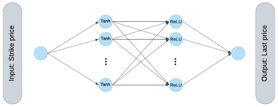
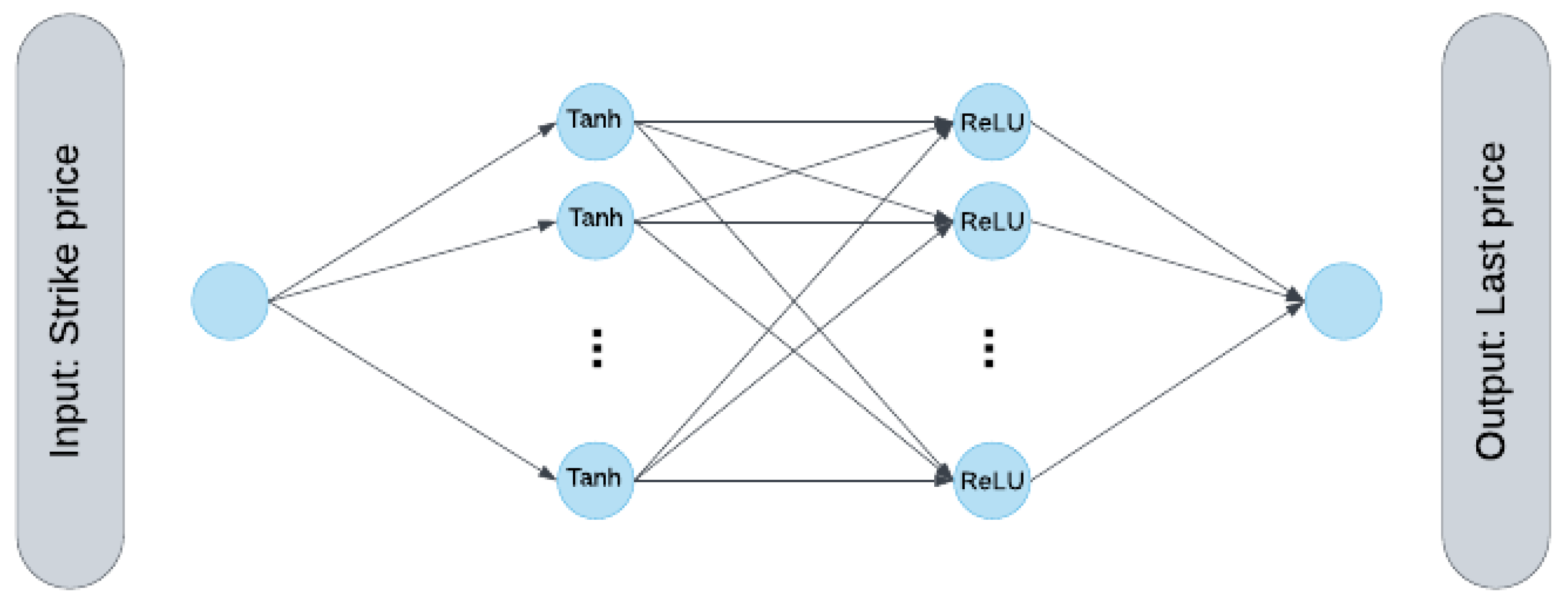
The first deep learning model, referred to as the PAN, is constructed to approximate the functional relationship between the strike price K and the last traded option price P. Formally, the network acts as a regression function $f:\mathbb{R}\to \mathbb{R}$, where the input is the strike price and the output is the estimated last price $\widehat{P}$.

The architecture comprises multiple layers that progressively transform the input into a meaningful price prediction:

• Input Layer: Accepts the strike price K as input;
• First Hidden Layer: Applies an affine transformation followed by the hyperbolic tangent activation:

  $$h^{\left(1\right)}=\tanh (W^{\left(1\right)}K+b^{\left(1\right)}),$$

  where $W^{\left(1\right)}\in {\mathbb{R}}^{8\times 1}$, $b^{\left(1\right)}\in {\mathbb{R}}^8$, and $h^{\left(1\right)}\in {\mathbb{R}}^8$;
• Second Hidden Layer: Applies a ReLU activation to the transformed features:

  $$h^{\left(2\right)}=\max (0,W^{\left(2\right)}{h}^{\left(1\right)}+b^{\left(2\right)}),$$

  where $W^{\left(2\right)}\in {\mathbb{R}}^{8\times 8}$ and $b^{\left(2\right)}\in {\mathbb{R}}^8$;
• Output Layer: Outputs the predicted price:

  $$\widehat{P}=W^{{\left(3\right)}^T}{h}^{\left(2\right)}+b^{\left(3\right)},$$

  where $W^{\left(3\right)}\in {\mathbb{R}}^8$, $b^{\left(3\right)}\in \mathbb{R}$.

This yields the complete model:

$$\widehat{P}=W^{{\left(3\right)}^T}\max (0,W^{\left(2\right)}\tanh (W^{\left(1\right)}K+b^{\left(1\right)})+b^{\left(2\right)})+b^{\left(3\right)}.$$

Figure 1 illustrates the PAN architecture and its forward data flow.

7.2. Calibration Correction Network

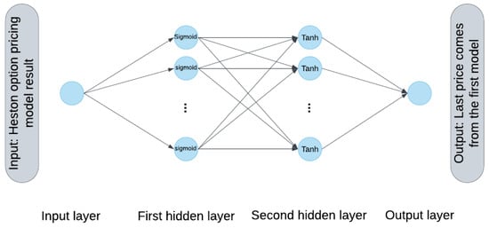
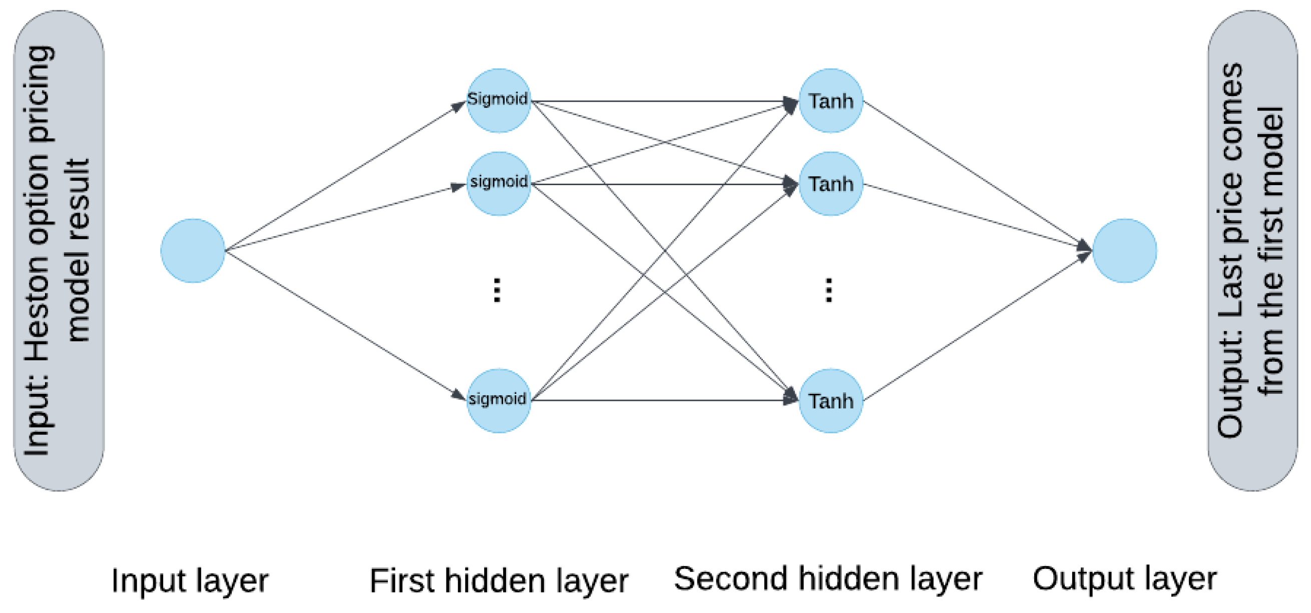
The second model, termed the CCN, is designed to refine the pricing output of the calibrated Heston model. Given the Heston-predicted price $P_{\mathrm{Heston}}$, the CCN maps this value to a more accurate estimate ${\widehat{P}}_{\mathrm{final}}$, effectively minimizing discrepancies between theoretical and observed market prices.

Its architecture is defined as follows:

• Input Layer: Takes $P_{\mathrm{Heston}}$ as input.
• First Hidden Layer: Applies a sigmoid activation:

  $$h^{\left(1\right)}=\sigma (W^{\left(1\right)}{P}_{\mathrm{Heston}}+b^{\left(1\right)}),$$

  with $W^{\left(1\right)}\in {\mathbb{R}}^{7\times 1}$, $b^{\left(1\right)}\in {\mathbb{R}}^7$;
• Second Hidden Layer: Applies the tanh activation:

  $$h^{\left(2\right)}=\tanh (W^{\left(2\right)}{h}^{\left(1\right)}+b^{\left(2\right)}),$$

  with $W^{\left(2\right)}\in {\mathbb{R}}^{7\times 7}$, $b^{\left(2\right)}\in {\mathbb{R}}^7$;
• Output Layer: Produces the corrected price estimate:

  $${\widehat{P}}_{\mathrm{final}}=W^{{\left(3\right)}^T}{h}^{\left(2\right)}+b^{\left(3\right)},$$

  where $W^{\left(3\right)}\in {\mathbb{R}}^7$, $b^{\left(3\right)}\in \mathbb{R}$.

The complete expression for the CCN becomes:

$${\widehat{P}}_{\mathrm{final}}=W^{{\left(3\right)}^T}\tanh (W^{\left(2\right)}\sigma (W^{\left(1\right)}{P}_{\mathrm{Heston}}+b^{\left(1\right)})+b^{\left(2\right)})+b^{\left(3\right)}.$$

Figure 2 shows the architecture and data flow within the CCN.

Traditional calibration methods often fail to accurately capture the nonlinear relationships between parameters in the Heston model, especially under volatile market regimes. Deep learning models such as PAN and CCN offer flexible function approximation capabilities and adapt to complex data structures without requiring explicit assumptions.

The PAN provides a reliable proxy for market data, while the CCN enhances theoretical model alignment. Together, these networks form a robust and efficient calibration pipeline, improving parameter estimation and ultimately enabling more accurate option pricing in practice.

7.3. Activation Function Selection

The activation functions employed in the PAN and CCN were selected in light of the distinct functional roles of these two components within the calibration framework. Although both networks are shallow fully connected architectures, they serve fundamentally different objectives: PAN approximates the option pricing surface, whereas CCN refines the baseline Heston-implied prices through systematic correction.

For PAN, which learns the mapping between strike price and observed option values, the target function is smooth, convex, and exhibits varying curvature across moneyness regions. To capture these characteristics effectively, a mixed activation structure was adopted. The first hidden layer uses the tanh activation, which is symmetric and continuously differentiable, making it well suited for modeling smooth global nonlinearities. Because inputs are standardized prior to training, tanh operates in a numerically stable regime and captures the overall curvature of the pricing surface efficiently. The second hidden layer employs the ReLU activation, introducing piecewise-linear flexibility that enables the representation of localized slope variations, particularly in the at-the-money region where price sensitivity changes more rapidly. In addition, ReLU facilitates stable gradient propagation and mitigates potential vanishing-gradient effects associated with purely saturating activations. The tanh–ReLU combination therefore balances smooth global approximation with localized expressiveness.

In contrast, CCN is designed to learn a correction function applied to Heston-implied prices. Rather than reconstructing the full pricing surface, it produces controlled residual adjustments. Consequently, bounded and smooth activation functions are more appropriate. The first hidden layer employs a sigmoid activation to constrain intermediate representations within a finite range, thereby promoting numerical stability and preventing extreme correction responses. The second hidden layer uses tanh, allowing symmetric positive and negative adjustments while maintaining smoothness. Since the correction may increase or decrease the baseline model price, a symmetric activation is appropriate at this stage. The sigmoid–tanh configuration thus ensures that the correction remains stable, smooth, and economically coherent.

Preliminary experiments with uniform activation schemes (e.g., exclusively ReLU or exclusively tanh) did not yield statistically significant improvements in RMSE or MAE and, in some cases, resulted in slightly less stable training dynamics. Accordingly, the mixed activation configuration was retained to achieve an appropriate balance between expressive capacity, numerical stability, and controlled correction behavior.

7.4. Mathematical Framework for Deep Learning-Based Calibration

To formalize the calibration procedure, we define the objective function as the weighted mean squared error between model-predicted and market-observed option prices. Given a set of market data indexed by maturity $T_i$ and log-moneyness $m_j$, and a neural network with trained weights $\widehat{W}$, the calibration problem can be expressed as:

$$\widehat{\eta }=\arg \underset{\eta \in \mathcal{H}}{\min }\sum _{i,j}{\omega }_{i,j}{\left(F(\widehat{W},{\eta }_i,T_i,m_j)-V^{\mathrm{Mkt}}(T_i,m_j)\right)}^2.$$

The proposed framework leverages two neural networks to improve pricing accuracy. The PAN is trained to approximate the mapping between strike price K and the last traded option price ${\widehat{P}}_{\mathrm{PAN}}\left(K\right)$. Subsequently, the CCN refines the output of the calibrated Heston model by learning a correction function:

$${\widehat{P}}_{\mathrm{final}}=\mathrm{CCN}\left(P_{\mathrm{Heston}}\right).$$

This two-stage architecture enables the model to first emulate the option price surface from data (via PAN) and then enhance calibration precision by correcting discrepancies (via CCN), even when traditional calibration is suboptimal.

To quantify the performance of both approaches, we compute standard error metrics including Root Mean Squared Error (RMSE), Mean Absolute Error (MAE), and Mean Relative Error (MRE), defined respectively as:

$$\begin{array}{cc}\hfill \mathrm{RMSE}& =\sqrt{{\displaystyle \frac{1}{N}}\sum _{i=1}^N{\left(P_i^{\mathrm{model}}-P_i^{\mathrm{market}}\right)}^2},\hfill \\ \hfill \mathrm{MAE}& ={\displaystyle \frac{1}{N}}{\displaystyle \sum _{i=1}^N}\left|P_i^{\mathrm{model}}-P_i^{\mathrm{market}}\right|,\hfill \\ \hfill \mathrm{MRE}& ={\displaystyle \frac{1}{N}}{\displaystyle \sum _{i=1}^N}{\displaystyle \frac{\left|P_i^{\mathrm{model}}-P_i^{\mathrm{market}}\right|}{P_i^{\mathrm{market}}}}.\hfill \end{array}$$

These metrics provide a comprehensive assessment of model accuracy across different pricing levels and moneyness intervals. The following figures and tables illustrate how the proposed deep learning framework achieves lower calibration errors compared to the traditional method.

8. Empirical Results and Analysis

This section evaluates the performance of the proposed two-phase deep learning framework for calibrating the Heston stochastic volatility model. We assess the accuracy and robustness of the methodology by comparing its performance against traditional calibration techniques.

To ensure the generalizability of our results, we conduct an extensive analysis using both in-sample and out-of-sample datasets. We quantify calibration accuracy by comparing model-implied prices with observed market data using standard metrics, including MSE, MAE, and MRE, which provide insights into the predictive consistency of the deep learning-enhanced Heston model.

Before presenting these quantitative findings, we detail the data construction and preprocessing procedures used in our empirical evaluation.

• Dataset construction and preprocessing: To ensure transparency and reproducibility, our dataset construction integrates both real-market observations and synthetic samples generated via the Heston model. The real-market data comprises European call options on the S&P 500, NASDAQ-100, and VIX indices. We selected strikes to ensure representative coverage across in-the-money, at-the-money, and out-of-the-money contracts, with times to maturity normalized as fractions of a trading year (e.g., 53/252 for 53 trading days). We excluded illiquid contracts and observations with missing or inconsistent prices. Finally, we removed extreme outliers to prevent the neural networks from overfitting to anomalous market quotes.
• Normalization and data split: All input features (strike, moneyness, and time to maturity) and the output variable (option price) were standardized by subtracting the training-set mean and dividing by the corresponding standard deviation. This scaling improves numerical stability during training and enforces consistent units across the training, validation, and test sets. The dataset was randomly shuffled and partitioned such that approximately 75–80% of contracts were used for training, with the remaining observations reserved for validation/testing. The split was implemented to maintain representative coverage across strikes and maturities, enabling a robust evaluation of out-of-sample performance.
• Parameter bounds: To allow sufficiently flexible yet controlled optimization, we calibrated the Heston parameters within explicit admissible bounds. Specifically, the risk-free rate was constrained to $r\in [0,1]$, the correlation between the two Brownian motions to $\rho \in [-1,1]$, and the remaining parameters—the mean-reversion speed $\kappa$, the long-run variance $\theta$, the volatility of volatility $\sigma$ (denoted by $\xi$ in some formulations), and the initial variance $v_0$—were each restricted to the interval $[0,10]$.

Unless stated otherwise, the empirical results reported below are computed on these datasets; we additionally provide a detailed case study for S&P 500 options on 7 February 2025.

In addition to calibration accuracy, we also examine the computational efficiency of the proposed framework, since practical deployment requires both reliable pricing performance and rapid recalibration.

To evaluate the computational efficiency of the proposed PAN–CCN framework, we recorded both the offline training time and the online inference (calibration) time. All wall-clock timing experiments were conducted on Google Colab using a Tesla T4 GPU. The offline stage, which is performed once for each data set, includes network training for the PAN and CCN components. In our implementation, this training phase required approximately 1 to 2 min per data set.

Once training is completed, the online calibration stage is highly efficient. The forward-pass evaluation of the trained PAN, followed by the CCN-based correction, requires less than 2 s per calibration instance. By contrast, the conventional Heston calibration procedure, implemented through SciPy’s minimize routine to iteratively minimize the pricing error, required approximately 30 s per calibration under the same computational environment.

Although the neural networks are trained separately for each data series, the inference cost of the trained models is negligible relative to repeated numerical optimization. Therefore, in settings where recalibration must be performed frequently, the proposed framework offers a clear computational advantage by shifting the majority of the workload to an offline stage. Overall, the PAN–CCN method achieves improved calibration accuracy while maintaining competitive—and, in repeated-use scenarios, substantially more efficient—computational performance.

We now turn to the empirical calibration results and illustrate the practical behavior of the proposed framework through a representative market case study.

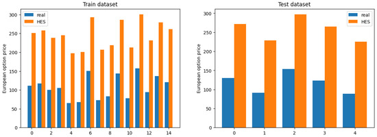
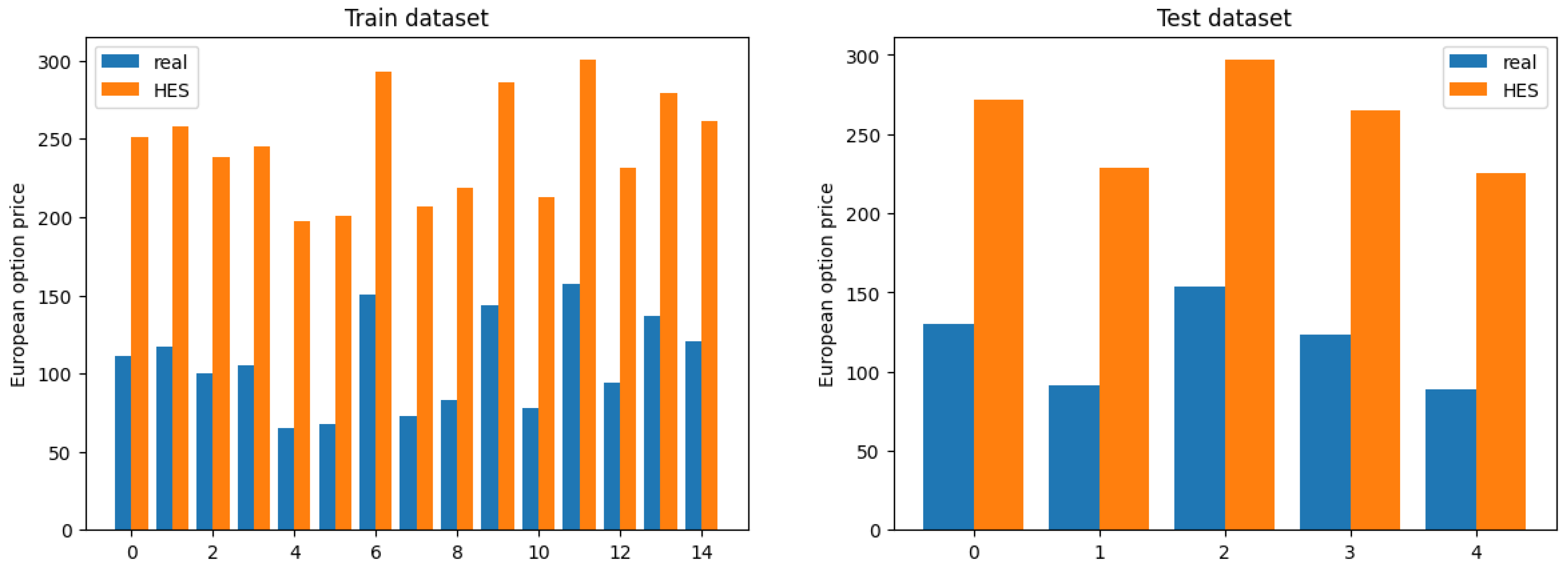
As part of the empirical study, we analyze European option prices on the S&P 500 index as of 7 February 2025, with the underlying asset priced at $6025.99. The analysis focuses on near-term options expiring within three days, utilizing the latest available market data from the final trading session. The calibration results are presented in Figure 3, which highlights the observed deviations between market option prices and those produced by the Heston model under conventional calibration methods.

These discrepancies underscore the limitations of traditional approaches in capturing the complex dynamics of market prices, particularly under short-term volatility conditions. The findings demonstrate the necessity for advanced calibration strategies—such as those employing deep neural networks—to reduce pricing errors and enhance the model’s alignment with real-world market behavior.

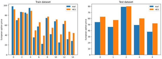
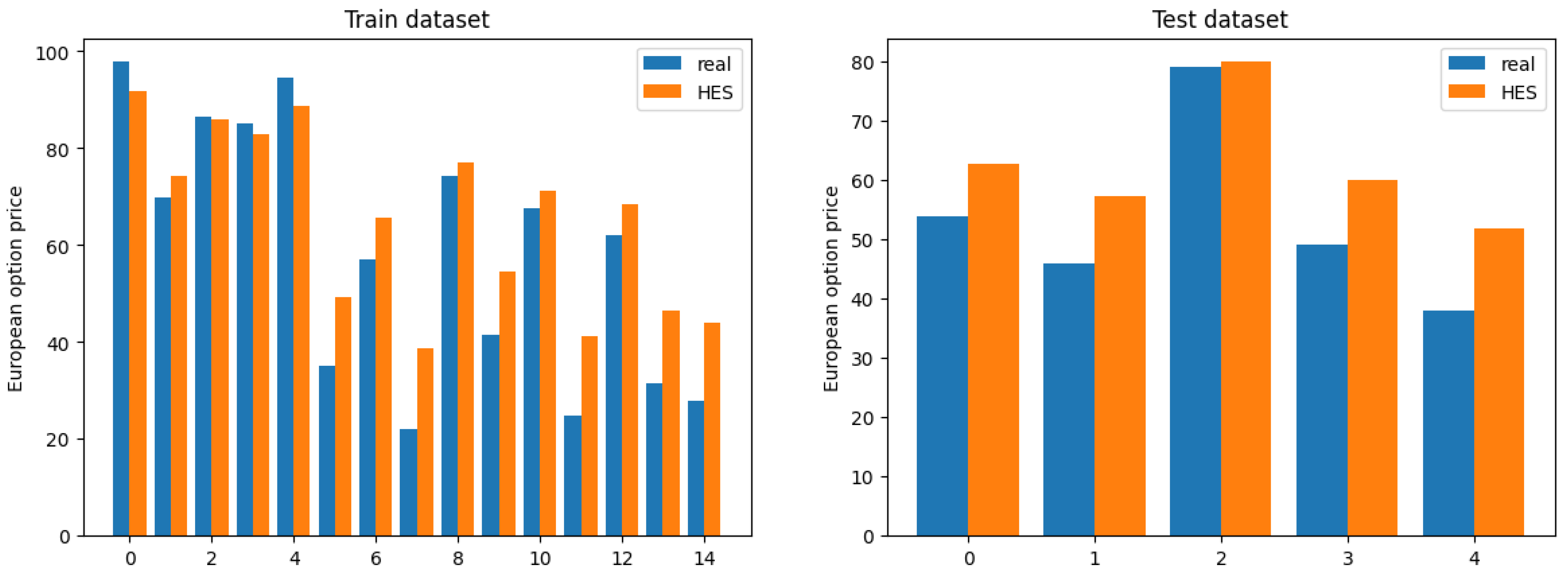
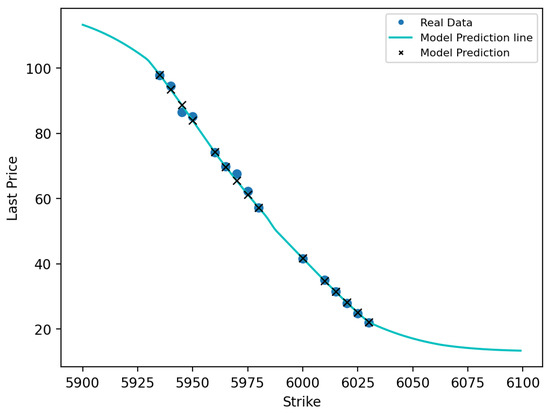
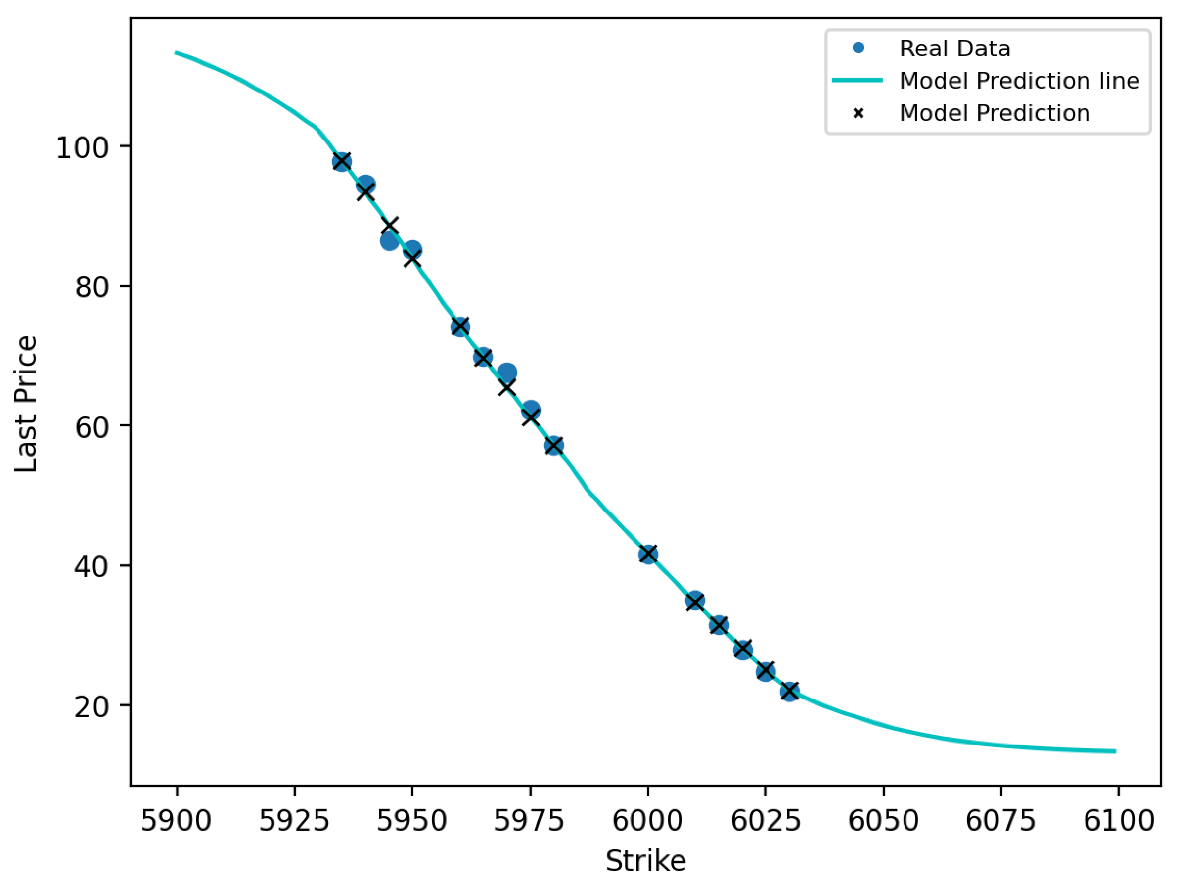
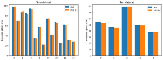
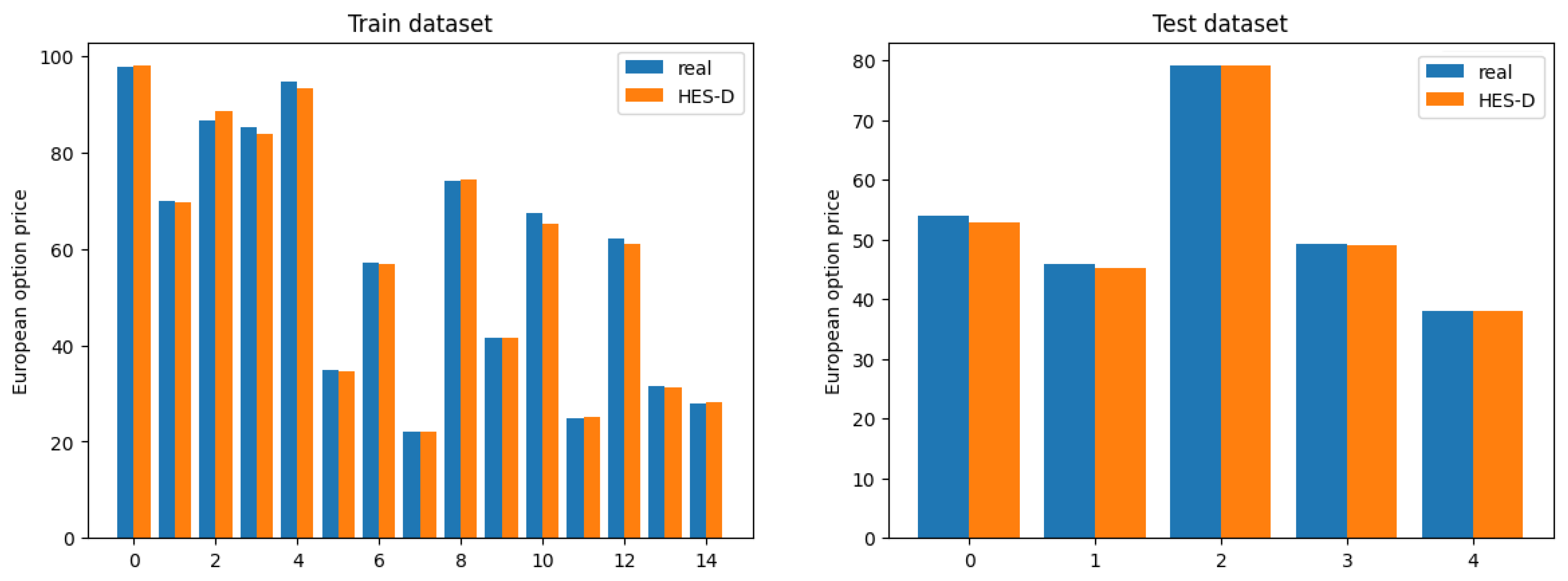
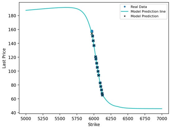
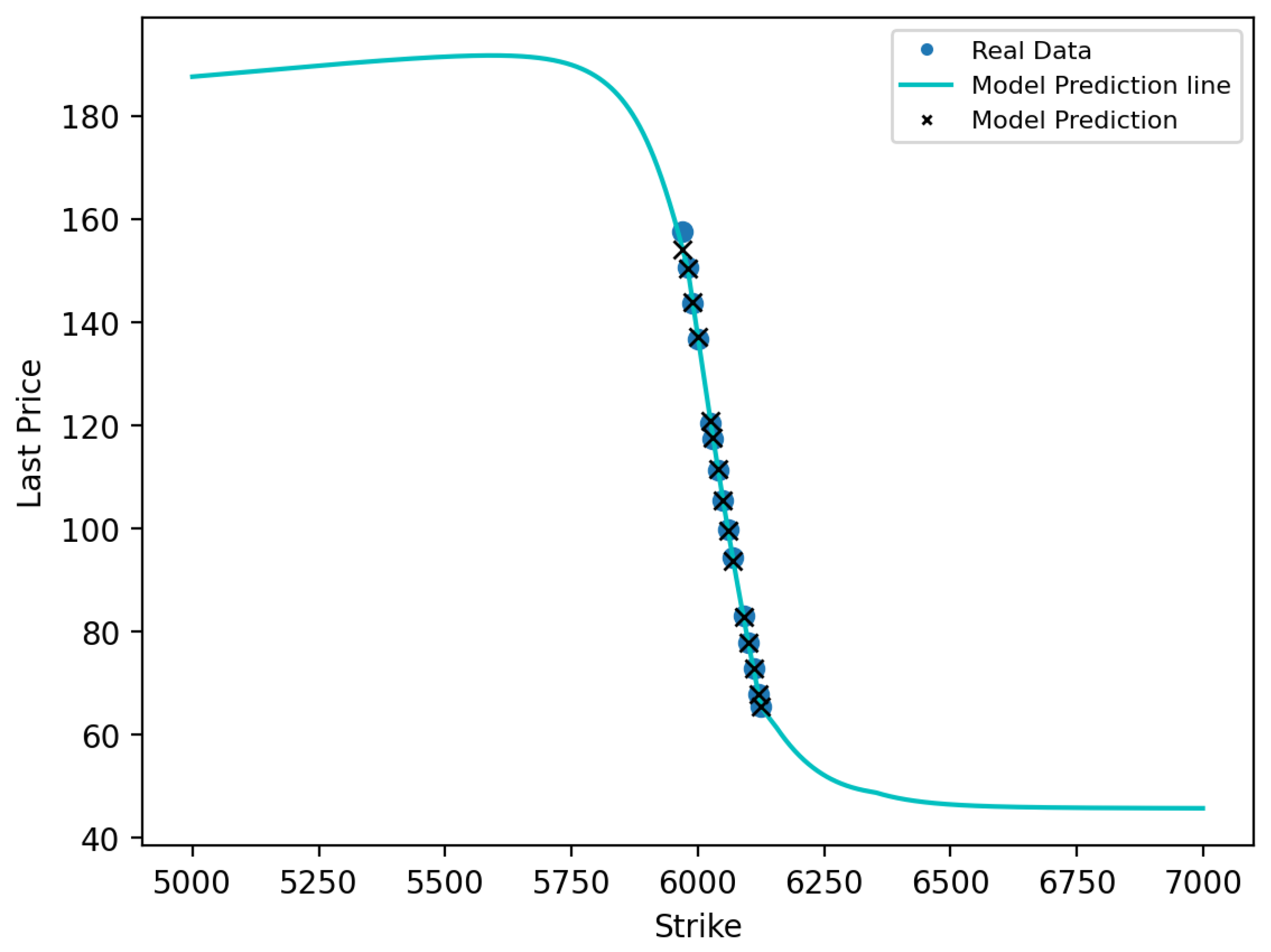
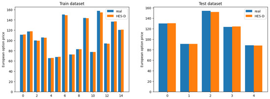
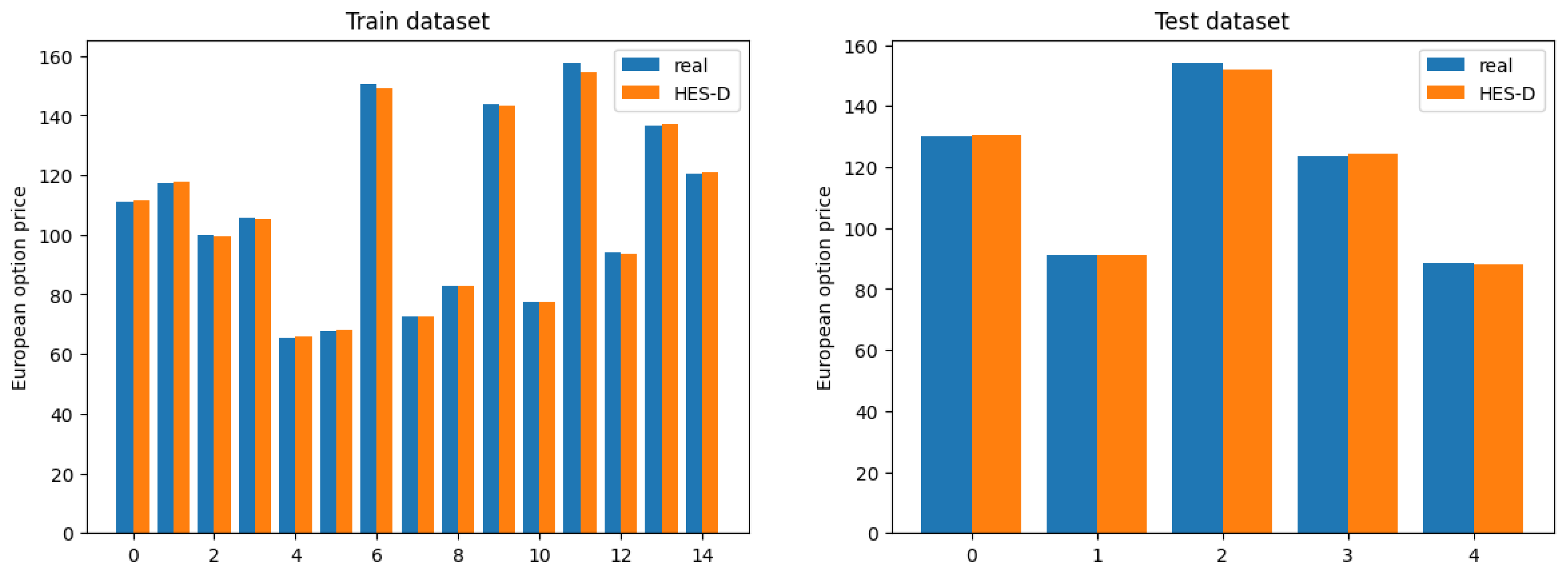
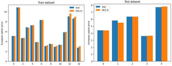
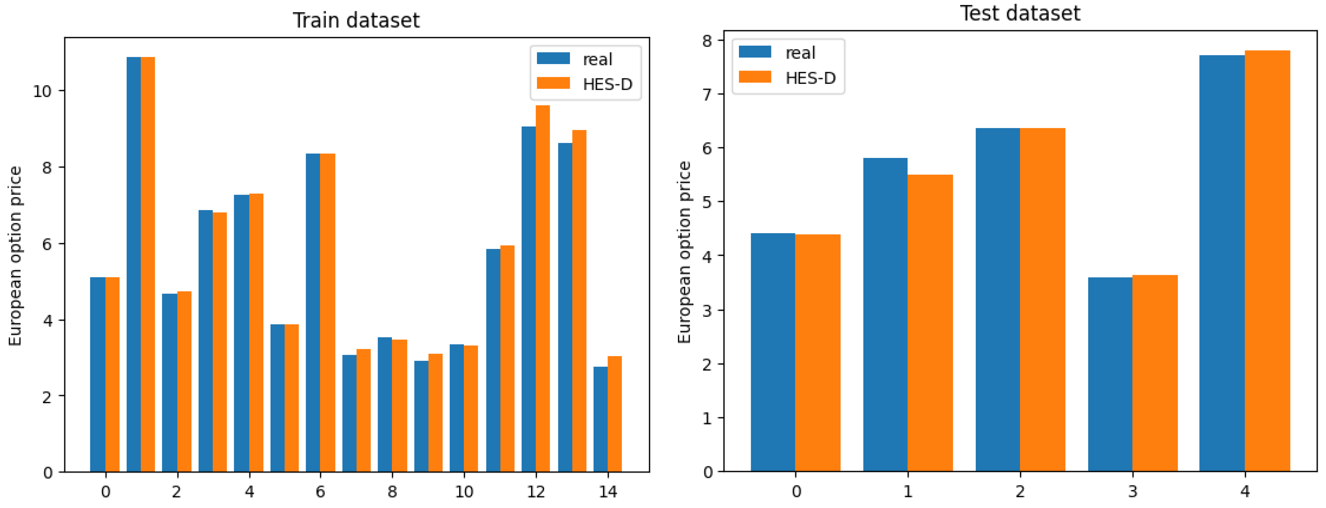
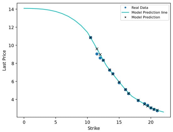
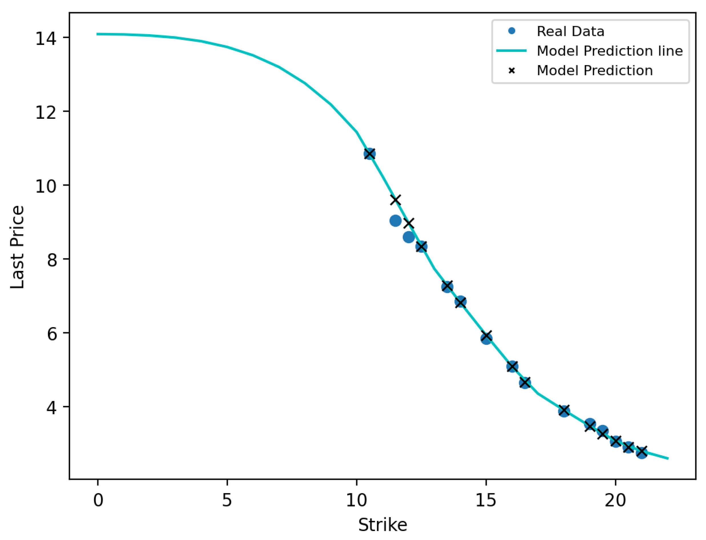
The PAN is first employed to estimate a smooth pricing curve for the last traded prices of $S\&P$ 500 options, using in-sample data. The results of this estimation are depicted in Figure 4, which demonstrates the network’s ability to accurately capture the underlying pricing structure. Building on this approximation, the CCN is subsequently trained using both the PAN-derived price surface and the preliminary calibration outputs from the Heston model. The goal is to refine these outputs and reduce systematic discrepancies. The enhanced pricing performance achieved through this correction mechanism is illustrated in Figure 5, clearly indicating that the proposed deep learning-enhanced calibration framework outperforms the traditional approach. To further substantiate this improvement, error metrics such as MSE and MAE are reported in

Table 1. Error metrics for $S\&P$ 500 data calibration.

Metric	Traditional	Deep Learning
Train RMSE	10.47	0.98
Train MRE	0.2515	0.0101
Train MAE	8.81	0.65
Test RMSE	10.21	0.55
Test MRE	0.2023	0.0079
Test MAE	9.20	0.39

, validating the superior performance of the deep learning-augmented approach over conventional calibration techniques.

The calibration of the Heston model is formulated as a nonlinear constrained optimization problem in which the objective is to minimize the weighted RMSE between model-implied option prices and observed market prices. Conventional calibration procedures typically rely on numerical optimization methods, which may become computationally expensive in nonlinear settings with multiple interacting parameters.

For the "Traditional" benchmark reported in this study, we employ the Sequential Least Squares Programming (SLSQP) algorithm implemented in the SciPy library. SLSQP is a standard gradient-based constrained optimization method that permits the direct incorporation of both parameter bounds and nonlinear restrictions. In particular, the calibration is performed under the Feller condition, $2\kappa \theta \ge {\xi }^2$, together with additional economically meaningful admissibility bounds on the parameter space.

The optimization is initialized from a stable reference starting point and run for at most 1000 iterations, with both function and parameter tolerances fixed at $1\times {10}^{-6}$. This specification is intended to provide a transparent and reproducible benchmark corresponding to a standard practical calibration workflow, rather than a heavily tuned multi-start global search procedure. All results reported for this baseline are consistent with the accompanying implementation.

As demonstrated in Table 1, the deep learning-based framework significantly outperforms the traditional calibration method across all error metrics. On the training set, the deep learning approach achieves notably lower values for RMSE ($0.98$ vs. $10.47$), MRE ($0.0101$ vs. $0.2515$), and MAE ($0.65$ vs. $8.81$), indicating a much closer alignment with observed market prices. The model maintains this superior performance on the test set, achieving an RMSE of $0.55$, substantially lower than the traditional method’s $10.21$, alongside similar improvements in MRE and MAE. These results affirm the effectiveness of the proposed approach in refining the calibration of the Heston option pricing model.

To assess the generalizability of the deep learning framework, we extend the analysis to a different data set—$S\&P$ 500 Mini options, with 39 days to expiration, evaluated as of 20 March 2025 (with calibration conducted on 7 February 2025). At this point, the underlying index value is $6049.50. We first apply the traditional calibration approach to this new data set, with the resulting model-generated option prices presented in Figure 6. This step provides a baseline for comparison, particularly in scenarios involving longer maturities and different market regimes.

Next, the PAN is applied to the $S\&P$ 500 Mini data set to learn a smoothed representation of the observed option price surface (see Figure 7). Building upon this, the CCN is trained to adjust the outputs of the initial Heston calibration, resulting in a refined price estimation. The improved performance of this combined method is illustrated in Figure 8. For a quantitative evaluation,

Table 2. Error metrics for $S\&P$ 500 Mini data calibration.

Metric	Traditional	Deep Learning
Train RMSE	138.60	0.89
Train MRE	1.39	0.005
Train MAE	138.55	0.56
Test RMSE	140.11	1.02
Test MRE	1.24	0.006
Test MAE	140.09	0.78

compares the deep learning-enhanced approach with the traditional method across multiple accuracy metrics. The results clearly show that the deep learning model maintains its superiority. On the training set, the RMSE, MRE, and MAE are dramatically reduced to $0.89$, $0.005$, and $0.56$ respectively, compared to the traditional method’s $138.60$, $1.39$, and $138.55$. This performance gap persists in the test set, where the deep learning model achieves an RMSE of $1.02$ versus $140.11$ for the traditional method. These findings underscore the robustness and adaptability of the proposed deep learning framework, particularly in capturing option price dynamics across varying maturities and market environments.

Extended Out-of-Sample Validation and Error Analysis

To further evaluate the robustness of the proposed PAN–CCN framework, we conducted additional out-of-sample experiments on assets beyond the S&P 500. Specifically, we evaluated the methodology on NASDAQ-100 index options and VIX options, which represent different underlying structures and pricing scales.

We consider European call options on the NASDAQ-100 index as of 21 February 2026, with expiration on 2 March 2026 (10 days to maturity). The underlying index level at the evaluation date was 24,984.65. The quantitative results are reported in

Table 3. Out-of-sample calibration performance on NASDAQ-100 European call options (21 February 2026; maturity: 2 March 2026).

Method	Train			Test
	RMSE	MAE	MRE	RMSE	MAE	MRE
Classical Heston	149.8603	147.7591	2.1805	126.4693	117.8126	4.3027
PAN–CCN	9.7467	5.6477	0.0470	48.3769	27.1886	0.2820

.

Under classical Heston calibration, the test RMSE is 126.4693 and the test MAE is 117.8126. After applying the PAN–CCN correction, the test RMSE decreases to 48.3769 and the test MAE to 27.1886. This corresponds to a substantial reduction in absolute pricing errors. A similar improvement is observed in relative error (MRE), which decreases from 4.3027 to 0.2820 on the test set.

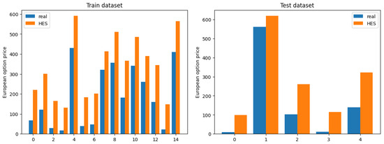
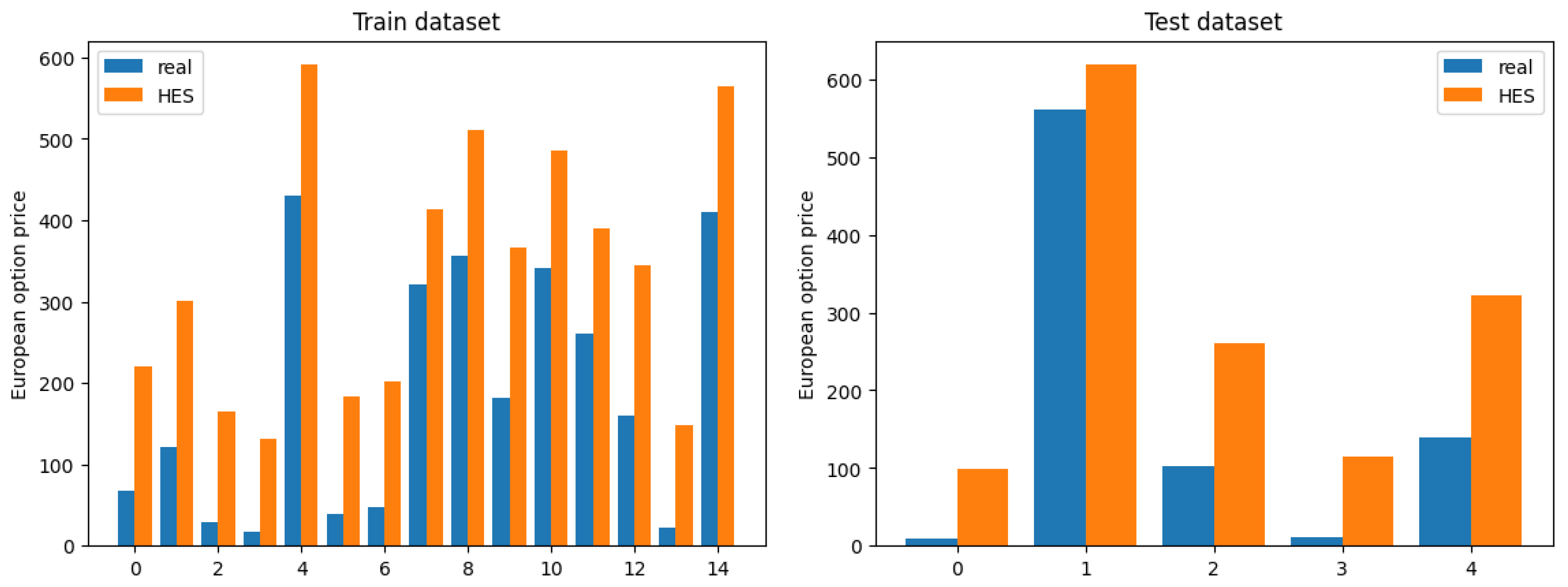
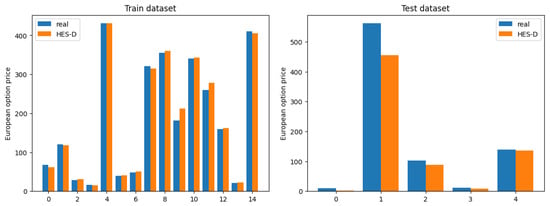
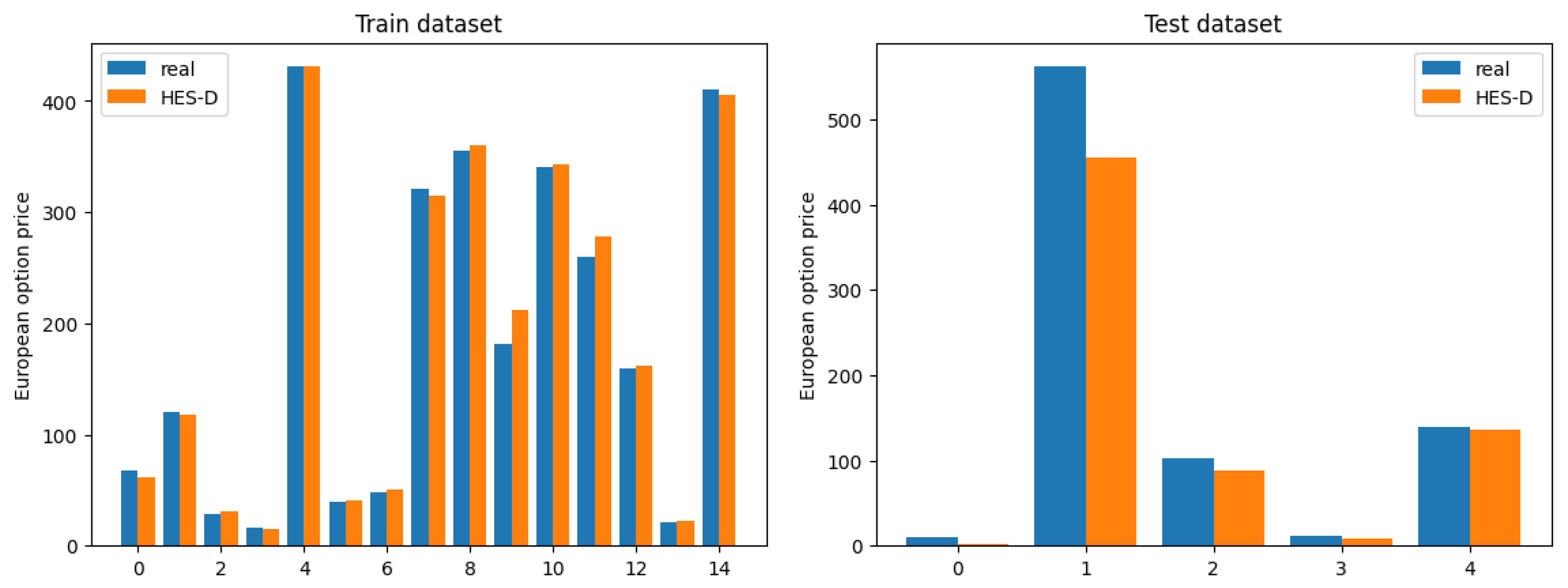
Figure 9 shows that, under classical calibration, noticeable deviations between model and market prices occur across several strikes in the test sample. In particular, the largest discrepancies appear in higher-priced contracts, where the absolute deviations are visually larger. After applying the neural network correction (Figure 10), the gap between model and market prices narrows visibly across all reported strikes. While residual errors remain, their magnitude is consistently smaller than in the baseline case, which is consistent with the quantitative improvements reported in Table 3.

Since the reported strikes span in-the-money, at-the-money, and out-of-the-money regions, the graphical comparisons provide a visual assessment of error behavior across different moneyness levels. The reduction in deviations after applying PAN–CCN is observed across the strike range rather than being confined to a narrow subset of contracts.

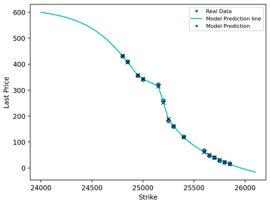
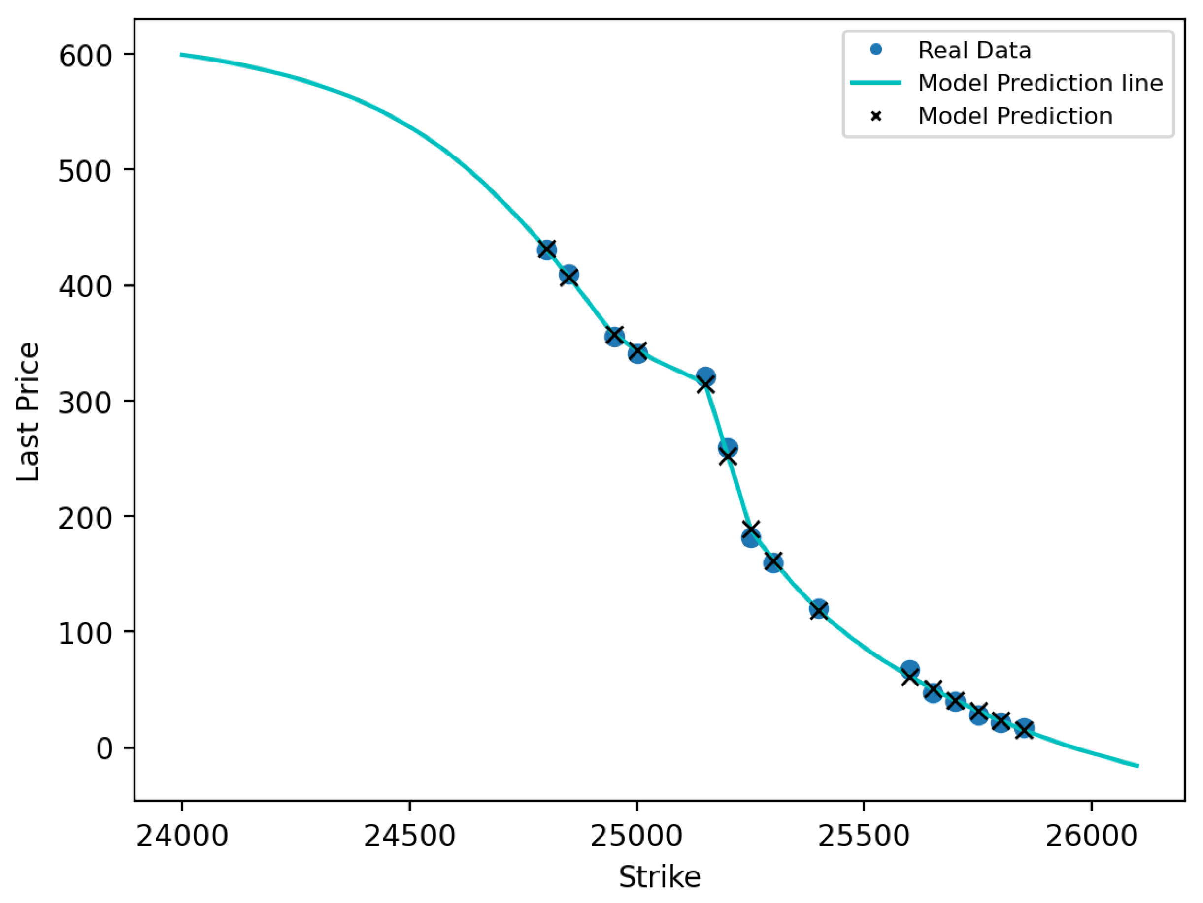
The PAN approximation shown in Figure 11 exhibits a smooth and monotonic relationship between strike and option price. The corrected pricing curve remains visually smooth and does not display irregular local fluctuations.

We additionally consider VIX European call options as of 21 February 2026, with expiration on 15 April 2026 (53 days to maturity). The VIX level at the evaluation date was 19.09. The corresponding results are summarized in

Table 4. Out-of-sample calibration performance on VIX European call options (21 February 2026; maturity: 15 April 2026).

Method	Train			Test
	RMSE	MAE	MRE	RMSE	MAE	MRE
Classical Heston	0.2479	0.1707	0.0304	0.2103	0.1736	0.0389
PAN–CCN	0.1986	0.1252	0.0262	0.1447	0.0907	0.0159

.

For classical calibration, the test errors are RMSE = 0.2103, MAE = 0.1736, and MRE = 0.0389. Using the PAN–CCN framework, the test errors improve to RMSE = 0.1447, MAE = 0.0907, and MRE = 0.0159 (Table 4).

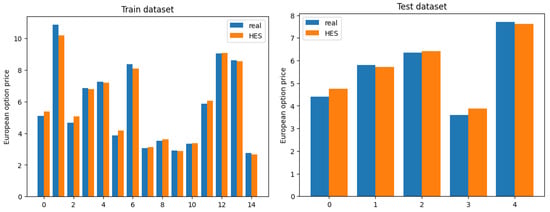
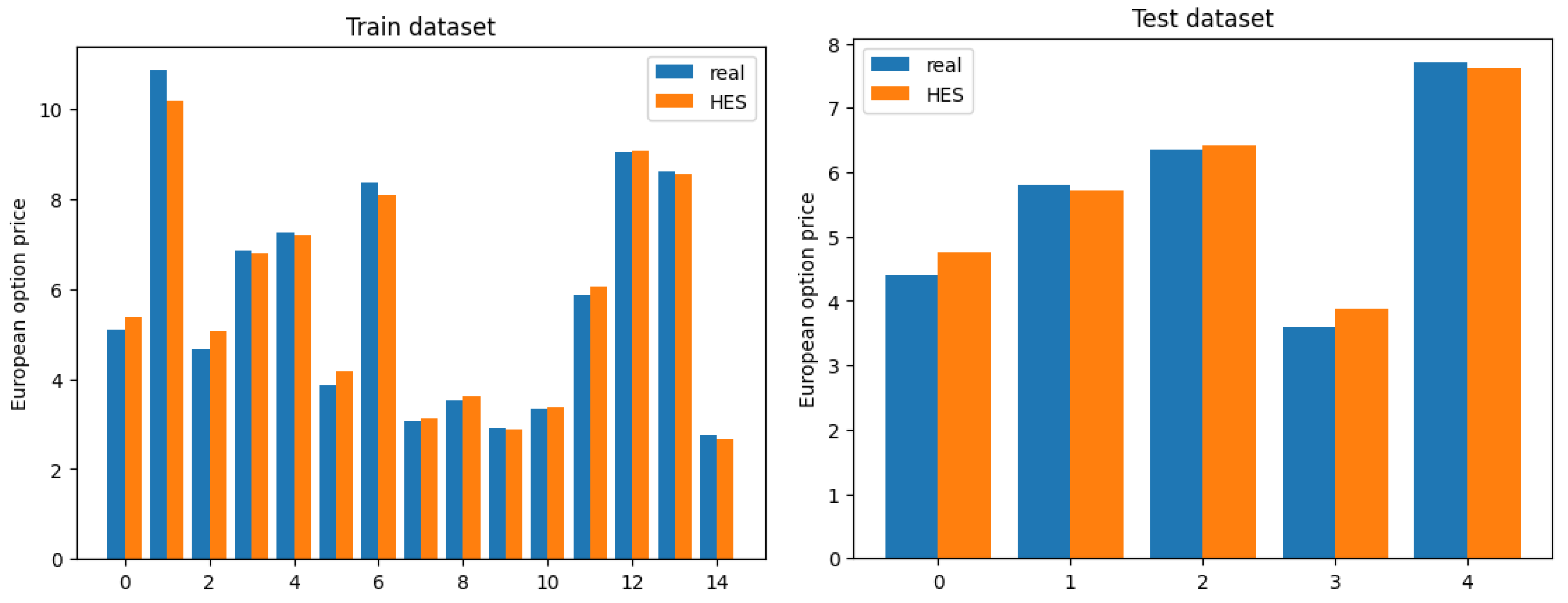
Figure 12 compares market prices and Heston-implied prices for the VIX sample, and Figure 13 shows the corresponding comparison after deep learning enhancement. In line with the reductions reported in Table 4, the corrected outputs in Figure 13 are visually closer to the market prices than the baseline results. Figure 14 presents the PAN approximation as a smooth fitted curve over strikes for this sample.

Although each asset is evaluated at a fixed maturity, the two datasets correspond to materially different time-to-maturity settings (10 days for NASDAQ-100 and 53 days for VIX), providing validation under distinct horizon lengths. Across both assets and their respective strike ranges, the improvements are not localized to a single pricing region but are observed broadly across the reported contracts.

Taken together, the numerical evidence in Table 3 and Table 4 and the graphical comparisons in Figure 9, Figure 10, Figure 11, Figure 12 and Figure 13 support the conclusion that the proposed framework improves out-of-sample calibration accuracy across distinct underlying assets and pricing regimes, while maintaining the overall smooth shape of the option price curve as illustrated in the figures.

Across all datasets considered, the proposed PAN–CCN framework attains consistently lower calibration errors than the classical Heston baseline in both in-sample and out-of-sample tests, as reflected by the RMSE, MAE, and MRE reported in Table 2, Table 3 and Table 4 and the error profiles in Figure 5, Figure 8, Figure 10, and Figure 13. These gains are consistent across diverse markets (S&P 500, NASDAQ-100, and VIX), indicating that the two-stage structure captures both the global shape of the price surface (via PAN) and systematic residual distortions (via CCN).

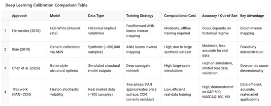
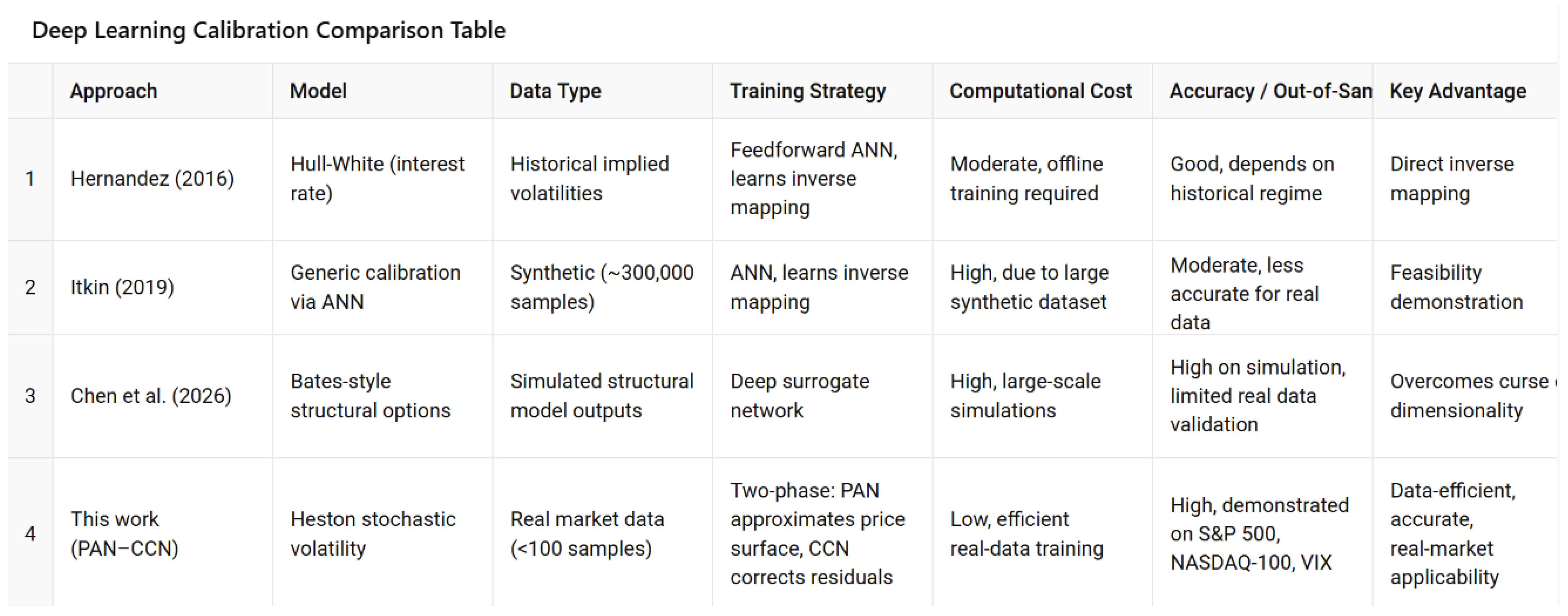
To further contextualize our contribution, Figure 15 summarizes the main empirical and data-regime differences between our approach and related neural calibration/surrogate frameworks. In contrast to Hernandez [17], which targets inverse mapping calibration in an interest-rate setting, and Itkin [18], which relies on large-scale synthetic training sets (on the order of $3\times {10}^5$ samples) to learn inverse mappings, our framework achieves strong calibration accuracy using fewer than 100 real-market samples. Compared with Chen et al. [19], whose deep surrogates are primarily trained on simulation-generated data for high-dimensional structural models, our emphasis is on data-efficient calibration and validation under real market observations, while maintaining computational efficiency suitable for practical deployment.

9. Conclusions

In this study, we developed a computationally efficient deep learning-enhanced calibration framework for the classical Heston stochastic volatility model. The proposed approach incorporated two regression-based neural networks: the Price Approximator Network (PAN), designed to approximate the option price surface as a function of contract characteristics, and the Calibration Correction Network (CCN), constructed to refine baseline Heston-implied prices by learning systematic residual structures relative to observed market prices.

The primary objective was to improve out-of-sample pricing performance while preserving computational efficiency. Empirical analyses conducted across heterogeneous assets—including equity index options (NASDAQ-100) and volatility index derivatives (VIX)—demonstrated that the proposed framework consistently reduced pricing errors relative to conventional calibration methods. The improvements were reflected in both absolute (RMSE, MAE) and relative (MRE) error metrics and remained stable across different market conditions.

The reduction in pricing error was observed across the option surface rather than being confined to isolated strike regions. In particular, the framework maintained strong performance across varying moneyness levels and maturities, including near-the-money and short-maturity contracts, where traditional calibration techniques often encounter numerical and optimization difficulties. This behavior indicates that the learned correction mechanism generalizes smoothly without introducing localized overfitting effects.

Overall, the results suggest that deep learning can be integrated with classical stochastic volatility models as a structured enhancement layer that improves calibration accuracy while retaining model interpretability. The cross-asset validation further indicates that the proposed architecture is sufficiently flexible to be extended to other stochastic volatility or jump–diffusion models, offering a practical framework for repeated calibration in modern financial environments.

References

- Heston, S.L. A closed-form solution for options with stochastic volatility with applications to bond and currency options. Rev. Financ. Stud. 1993, 6, 327–343. [Google Scholar] [CrossRef] [Scilit]
- Black, F.; Scholes, M. The pricing of options and corporate liabilities. J. Polit. Econ. 1973, 81, 637–654. [Google Scholar] [CrossRef] [Scilit] [PubMed]
- Gatheral, J. The Volatility Surface: A Practitioner’s Guide; John Wiley & Sons: Cambridge, UK, 2011. [Google Scholar]
- Duffie, D.; Pan, J.; Singleton, K. Transform analysis and asset pricing for affine jump–diffusions. Econometrica 2000, 68, 1343–1376. [Google Scholar] [CrossRef] [Scilit]
- Broadie, M.; Kaya, O. Exact simulation of stochastic volatility and other affine jump diffusion processes. Oper. Res. 2006, 54, 217–231. [Google Scholar] [CrossRef] [Scilit]
- Andersen, L.B.G. Efficient simulation of the Heston stochastic volatility model. J. Comput. Financ. 2007, 11, 1–42. [Google Scholar]
- Gneiting, T.; Balabdaoui, F.; Raftery, A.E. Probabilistic forecasts, calibration and sharpness. J. R. Stat. Soc. Ser. B 2007, 69, 243–268. [Google Scholar] [CrossRef] [Scilit]
- Heaton, J.B.; Polson, N.G.; Witte, J.H. Deep learning in finance. Annu. Rev. Financ. Econ. 2017, 9, 145–165. [Google Scholar]
- Goodfellow, I.; Bengio, Y.; Courville, A. Deep Learning; MIT Press: Cambridge, MA, USA, 2016. [Google Scholar]
- Gu, S.; Kelly, B.; Xiu, D. Empirical asset pricing via machine learning. Rev. Financ. Stud. 2020, 33, 2223–2273. [Google Scholar] [CrossRef] [Scilit]
- Hutchinson, J.M.; Lo, A.W.; Poggio, T. A nonparametric approach to pricing and hedging derivative securities. J. Financ. 1994, 49, 851–889. [Google Scholar] [CrossRef]
- Sirignano, J.; Cont, R. Universal features of price formation in financial markets: Perspectives from deep learning. Quant. Financ. 2019, 19, 1449–1459. [Google Scholar] [CrossRef] [Scilit]
- Ruf, J.; Wang, W. Neural networks for option pricing and hedging: A literature review. arXiv 2019, arXiv:1911.05620. [Google Scholar]
- Buehler, H.; Gonon, L.; Teichmann, J.; Wood, B. Deep hedging. Quant. Financ. 2019, 19, 1271–1291. [Google Scholar] [CrossRef] [Scilit]
- Christoffersen, P.; Heston, S.L.; Jacobs, K. Option valuation with conditional skewness in the Heston model. J. Financ. Econ. 2010, 98, 380–404. [Google Scholar]
- Horvath, B.; Muguruza, A.; Tomas, M. Deep learning volatility: A hybrid approach to pricing and calibration. Quant. Financ. 2021, 21, 657–675. [Google Scholar] [CrossRef] [Scilit]
- Hernandez, A. Model calibration with neural networks. SSRN Electron. J. 2016. Available online: https://ssrn.com/abstract=2812140 (accessed on 20 July 2016). [CrossRef] [Scilit]
- Itkin, A. Deep learning calibration of option pricing models: Some pitfalls and solutions. arXiv 2019, arXiv:1906.03507. [Google Scholar]
- Chen, H.; Didisheim, A.; Scheidegger, S. Deep surrogates for finance: With an application to option pricing. J. Financ. Econ. 2026, 177, 104222. [Google Scholar] [CrossRef] [Scilit]
- Cox, J.C.; Ingersoll, J.E.; Ross, S.A. A theory of the term structure of interest rates. Econometrica 1985, 53, 385–407. [Google Scholar] [CrossRef] [Scilit]
- Stein, E.M.; Stein, J.C. Stock price distributions with stochastic volatility: An analytic approach. Rev. Financ. Stud. 1991, 4, 727–752. [Google Scholar] [CrossRef] [Scilit]
- Liu, S.; Borovykh, A.; Grzelak, L.A.; Oosterlee, C.W. A neural network-based framework for financial model calibration. J. Math. Ind. 2019, 9, 9. [Google Scholar] [CrossRef] [Scilit]
- Bayer, C.; Horvath, B.; Muguruza, A.; Stemper, B.; Tomas, M. On deep calibration of (rough) stochastic volatility models. arXiv 2019, arXiv:1908.08806. [Google Scholar]
- Kingma, D.P.; Ba, J. Adam: A method for stochastic optimization. arXiv 2014, arXiv:1412.6980. [Google Scholar]
- Ferguson, R.; Green, A. Deeply learning derivatives. arXiv 2018, arXiv:1809.02233. [Google Scholar]
- Platon, R.; Dehkordi, V.R.; Martel, J. Hourly prediction of a building’s electricity consumption using case-based reasoning, artificial neural networks and principal component analysis. Energy Build. 2015, 92, 10–18. [Google Scholar] [CrossRef] [Scilit]
- Paszke, A.; Gross, S.; Massa, F.; Lerer, A.; Bradbury, J.; Chanan, G.; Killeen, T.; Lin, Z.; Gimelshein, N.; Antiga, L.; et al. PyTorch: An imperative style, high-performance deep learning library. Adv. Neural Inf. Process. Syst. 2019, 32, 8024–8035. [Google Scholar]
- He, K.; Zhang, X.; Ren, S.; Sun, J. Delving deep into rectifiers: Surpassing human-level performance on ImageNet classification. In Proceedings of the IEEE International Conference on Computer Vision; IEEE: New York, NY, USA, 2015; pp. 1026–1034. [Google Scholar]
- Nair, V.; Hinton, G.E. Rectified linear units improve restricted Boltzmann machines. In Proceedings of the 27th International Conference on Machine Learning; Omnipress: Madison, WI, USA, 2010; pp. 807–814. [Google Scholar]
- Glorot, X.; Bengio, Y. Understanding the difficulty of training deep feedforward neural networks. In Proceedings of the Thirteenth International Conference on Artificial Intelligence and Statistics; JMLR Workshop and Conference Proceedings; 2010; pp. 249–256. [Google Scholar]
Disclaimer/Publisher’s Note: The statements, opinions and data contained in all publications are solely those of the individual author(s) and contributor(s) and not of MDPI and/or the editor(s). MDPI and/or the editor(s) disclaim responsibility for any injury to people or property resulting from any ideas, methods, instructions or products referred to in the content. |
© 2026 by the authors. Licensee MDPI, Basel, Switzerland. This article is an open access article distributed under the terms and conditions of the Creative Commons Attribution (CC BY) license.